A network aggregation model for the dynamics and treatment of neurodegenerative diseases at the brain scale
Abstract
Neurodegenerative diseases are associated with the assembly of specific proteins into oligomers and fibrillar aggregates. At the brain scale, these protein assemblies can diffuse through the brain and seed other regions, creating an autocatalytic protein progression.
The growth and transport of these assemblies depend on various mechanisms that can be targeted therapeutically. Here, we use spatially-extended nucleation-aggregation-fragmentation models for the dynamics of prion-like neurodegenerative protein-spreading in the brain to study the effect of different drugs on whole-brain Alzheimer’s disease progression.
1 Introduction
The self-assembly of proteins into ordered linear structures plays a central role in the normal functioning of organisms, spanning from bacteria to mammals [1, 2], with unique mechanical properties also eliciting potential in industrial contexts [3, 4]. Recent interest in protein aggregation has led to an explosion in exploratory studies across a broad spectrum of disciplines. A particularly pressing motive for such research has more medical origins; the undesired filamentous aggregation of proteins can have severe repercussions on an organism’s well-being. In such contexts, aggregation is the defining mechanism driving a cascade of pathogenic proteins characteristic of various diseases. There are now approximately 50 disorders associated with a particular class of protein filaments, known as amyloids, with disparate symptoms ranging from non-neuropathic localized amyloidosis, such as type II diabetes, to neurodegenerative diseases such as Alzheimer’s disease (AD), Parkinson’s disease and Huntington’s disease [5]. Despite the diversity of pathogenic proteins involved in these disorders [6], experimental studies uncover commonalities in the underlying physicochemical and biochemical disease origins. This shared characteristic is the misfolding of normally soluble, functional peptides and proteins and their subsequent conversion into intractable aggregates [7]. Although only understood just decades ago neurodegenerative diseases are no longer rare, and are rapidly becoming among the most common and debilitating medical conditions in the modern world [8]. This growing problem poses significant challenges in modern healthcare, making any progress in our understanding of amyloid fibrillization crucial, holding implications for a wide range of debilitating medical conditions.
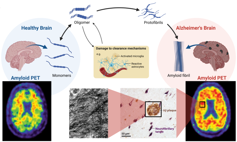
The AD brain has defining pathological features of cortical amyloid plaques, comprising a fibrillar form of the amyloid- protein (A) as depicted in Figure 1. It is thought that such A accumulation facilitates the subsequent cascade of neurofibrillary tangles (NFTs) from aggregated tau protein [9, 10]. Several hypotheses govern the deterministic modelling of protein accumulation and propagation in AD to gain meaningful estimates of its dynamics. First, the prion-like hypothesis [11, 12, 13, 14, 15] broadly postulates that neurodegenerative diseases result from an accumulation of misfolded forms of these proteins, which aggregate and contribute to neurodegenerative pathology. In this process, disease-specific misfolded proteins act as a template upon which healthy proteins misfold in a manner akin to prion formation [16], forming extensive chains transported through the brain along axonal pathways. Given that aggregates of differing sizes exhibit unique transport characteristics and varying toxicity levels, it is essential to monitor their spatial and temporal evolution independently. Second, the amyloid- hypothesis [17, 18, 19] establishes that amyloidogenic protein accumulation in AD could be causative, placing A central to disease pathology with supporting experimental evidence suggesting A as a primary driver of AD [20]. This hypothesis has guided most AD research over the past two decades and motivated the development of many therapeutic antibodies targeting different species of the A peptide [21]. In the last decade, 15 potential therapeutics targeting the role of A in AD in various ways, including inhibition of enzymes involved in A production and removal of A aggregates using antibodies, have been tested in phase III clinical trials [22]. However, the failure of most such drug trials and recent experimental evidence has renewed scrutiny of its foundational assumptions, arguing for the possible importance of other mechanisms. Moreover, an alternative theory, the A oligomer hypothesis, suggests that oligomers composed of small numbers of A peptides are the most relevant pathological A species, with amyloid plaques perhaps serving as a reservoir for such species [23, 24]. Consistent with this, next-generation therapeutic intervention strategies targeting low molecular weight oligomers of A are showing promise [25].
Another potential driving factor of AD is the clearance of misfolded proteins, a somewhat elusive and powerful in vivo effect which experiments in vitro fail to replicate. The production of tau and A peptides is a natural process related to neuronal activity. In a healthy brain, these standard metabolic waste by-products [26, 27] are removed from intracellular and extracellular compartments by several clearance mechanisms [28, 29]. Waste proteins are broken down by enzymes, removed by cellular uptake, crossing the blood–brain barrier, or effluxing to cerebrospinal fluid compartments, eventually reaching arachnoid granulations or the lymphatic vessels. Such healthy clearance mechanisms, working in harmony, avert the buildup of toxic A plaques and tau NFT, but their impairment or dysfunction can lead to AD pathology. The specific descriptions of in vivo clearance mechanisms remain a topic of clinical debate; however, the kinetics enabling toxic proteins to amass into pathological aggregates can be systematically studied in vitro and coupled to dynamic clearance mathematically to simulate the naturally therapeutic, or destabilising, effect of clearance and its response to toxic aggregate mass.
Studies of the history of medicine reveal that significant progress in preventing and treating a disease typically demands a deep understanding of its underlying causes [30]. Crucially, however, the molecular mechanisms underlying aggregate proliferation in the complex domain of the brain are still, like clearance mechanisms, poorly understood. The community acknowledges the need for a deeper understanding of molecular processes in vivo to achieve success in therapeutic strategies [22]. Moreover, as emphasised by Karran et al. (2022) [22], clear experiments of therapeutic hypotheses have been challenging to conduct with anti-A approaches: the target is not clearly defined (amyloid plaques, A oligomers, or monomers), the mechanism by which A affects cognition is unknown (direct or indirect synaptic toxicity, induction of tau pathology, neuroinflammation, or a combination of all and other effects), sometimes failures are attributed to drug administration at too late of a stage of neurodegeneration, and there is also evidence that amyloid removal is faster in patients with high baseline levels further confounding a direct comparison of antibodies [31]. Mathematical modelling can contribute to a deeper understanding of these problems and suggest new approaches. Significant progress have been made in elucidating the molecular mechanisms that occur during the assembly of purified protein molecules under controlled in vitro conditions. This advance results from new experimental methods as well as better theoretical models used to analyse the resulting data. Modelling these molecular mechanisms in a disease-relevant system, including in vivo effects such as clearance and transport at the brain scale, would provide invaluable insights to guide the design of potential cures for these devastating disorders.
The goal of this study is twofold. The primary focus is to develop and analyse, both analytically and computationally, new models to study protein aggregation kinetics, including in vivo effects such as clearance in a brain region locally, then scale up to include transport on the human connectome. Second, we use our new in vivo aggregation models to test the impact of potentially therapeutic monoclonal antibodies and inform optimal treatment strategies to maximise toxic mass clearance. Our general approach is to study the size distribution of A aggregates, with parameters informed by experiments in a HEPES buffer [25], both locally and brain-wide using discrete aggregation equations [34, 35, 36], finding analytical relationships where possible and solving numerically on the brain’s connectome. The novelty of our work is exploring how the known in vitro aggregate size dynamics and the pharmodynamic effect of drugs [25, 37] scales up to affect the progression of neurodegenerative diseases in a more realistic in vivo model at the brain scale, exploring a variety of clearance profiles reflective of treatment strategies. A primary result of interest to the computational biology and pharmaceutical community will be to demonstrate that the non-trivial in vivo effects of transport and clearance of oligomers are realized with relatively simple deterministic models and couplings, leading to effects with clear physiological interpretations in neurological disease modelling. Moreover, the mathematical analysis will highlight that clearance mechanisms are crucial in destabilizing the system towards proteopathy and potentially in restabilizing the system, with implications for therapeutic intervention within the complex domain of the human AD brain.
2 From microscopic models to brain-scale dynamics
Protein aggregation pathways are complex and involve multiple steps with distinct rates [38]. Advancements based on chemical kinetics have produced a deep understanding of the fundamental mechanisms underlying the formation of aggregates in ideal conditions at the microscopic scale, thereby making clearer the potential for therapeutic intervention [39, 40]. Namely, a theoretical framework of the classic nucleated polymerisation theory supplemented with secondary aggregation pathways [41, 42, 43] has been combined with systematic in vitro experiments performed under differing conditions, such as varied concentration or pH [44, 45], to reveal such mechanisms.
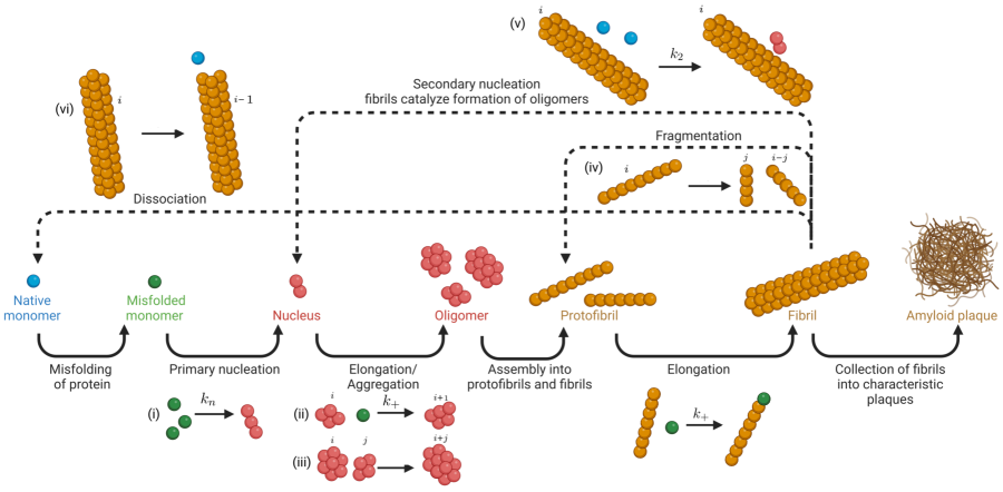
As shown in Figure 2, it is understood that A monomers misfold by seeding events or prion-like templating [46, 47, 48], followed by primary nucleation, which leads to the creation of a polymer of length soluble monomers. Filaments elongate and dissociate linearly from both ends with the addition and removal of monomers in a reversible manner. Oligomers and fibrils of different sizes also aggregate to form larger aggregates. Additionally, secondary pathways of fragmentation and monomer-dependent secondary nucleation lead to the creation of new fibril ends from pre-existing polymers.
At present, no brain-scale in vivo therapeutic intervention model accounts for the kinetics of protein aggregation. Leading therapeutic models are in vitro models for the impact of drugs on the aggregation process [25], or brain-wide compartmental models that broadly depict disease development in the presence of drugs over months but neglect the underlying kinetics of drug action [37]. We combine the aforementioned spatial and time scales, building upon insights from the Smoluchowski-type models of [49] and [35], which respectively capture the physiological effects of clearance and brain-wide neuronal transport of aggregates.
Our general approach is to start with a microscopic model with parameters validated experimentally by in vitro experiments and extend to both in vivo settings and over the entire brain.
First, the microscopic model that we start with has been carefully calibrated in a series of experiments. In particular, it has been shown that the main processes sufficient to explain the mass increase of oligomers are linear aggregation, primary, and secondary nucleation. Similarly, it has been shown that both depolymerisation and fragmentation can be ignored in the first instance.
Second, we extend the microscopic model to include in vivo mechanisms: the natural production of monomers, the clearance of monomers, and a general slowing down due to local cellular effects. This second model represents the local dynamics of oligomers in a given brain region.
Third, we extend the model to include spatial effects at the brain scale. This is performed by coupling different brain regions and assuming that proteins are mostly transported through the brain along axonal pathways. This final system belongs to the general class of network diffusion-aggregation-fragmentation models discussed in [35]. In this way, we derive an entirely mechanistic brain-wide network model of neurodegeneration in which we simulate and optimize therapeutic intervention.
2.1 A minimal microscopic model
Our minimal microscopic model for protein aggregation includes the following mechanisms: primary heterogeneous nucleation; secondary nucleation; linear elongation. Each aggregate of a given size is represented by a population. Let be the concentration of aggregates of size . Then, the microscopic master equations are:
| (1a) | |||
| (1b) | |||
| (1c) | |||
where
| (2) |
where is the concentration of monomers and the kinetic rate constants are defined in Table 1. Here, and are the first two moments of the population distribution; they represent the total number and total mass of aggregates, respectively.
| param. | mechanism | A42 HEPES [25] | units |
|---|---|---|---|
| primary nucleation | M h-1 | ||
| secondary nucleation | M-2h-1 | ||
| monomer saturation | M2 | ||
| mass saturation | M2 | ||
| elongation | M-1h-1 | ||
| initial monomer c. | M |
It is of interest, before we consider other effects, to understand the overall behavior of this system. This can be easily accomplished by looking at the moment equation obtained as a closed system for and :
| (3) | |||
| (4) | |||
| (5) |
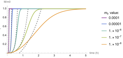
By construction, the total mass of the system is conserved and assuming and , we have for all time. As shown in Fig. 3, the behavior of this system is rather simple. The toxic mass increase from to in a sigmoid-like manner. Various approximations of this curve have been proposed and used for model validation and parameter fitting [50, 39, 51]. We observe that for large variations of the initial concentration, the dynamics saturates within hours.
To better understand the time scale involved in the process, we defined the halftime to be the the time at which an initial unseeded system reaches half of the final concentration . To approximate , we assume that is small compared to other rates and linearize the system (3– 4) with around . Expanding , where , we obtain, to first order
| (6) |
where
| (7) |
A very good approximation of the exact solution of this linear system with unseeded initial conditions is obtained by neglecting the fast decaying exponential:
| (8) |
The linear solution gives a reasonable estimate of the initial dynamics and is simple enough to provide an analytical estimate of the halftime:
| (9) |
In the range of parameters involved, we can further simplify this expression to
| (10) |
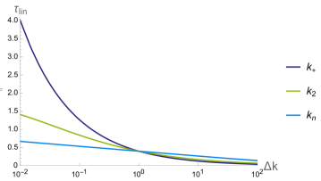
We now turn to the variation of time scales associated with the various parameters. We fix the initial concentration to M and systematically vary each parameter over four orders of magnitude around their values given in Table 1, to study which rate constant has the most effect on the dynamics. From (10), we see that variations in , or are equivalent as these parameters only enter as a product. As expected, the variations due to a reduction in the primary nucleation terms are weak (and only due to the logarithm), whereas reductions in (with a log dependence divided by a root) are faster and variations in dominate (as they depend only on the square root).
The overall conclusion is that the pure conversion process of a population of monomers into oligomers is governed in vitro by rate constants that provide a typical time scale of hours, even when kinetic rates are modified by orders of magnitude. However, we know that in vivo any neurodegenerative disease evolves on time scales of years or decades. Even in the case where all kinetic rates are reduced by a factor , the resulting new halftime is simply , which would require a factor of about to reach a time scale of a year. This apparent contradiction requires new mechanisms to explain the dramatic slowdown of these processes.
2.2 A local model including clearance, production, and saturation
Based on our understanding of the minimal in vitro model that represents a closed-system, we can now extend it to include effects that appear in vivo. First, we assume that there is a regulation mechanism for the production of monomers such that their concentration remains mostly constant, despite their uptake in the formation of larger structures. Therefore, within the modelling framework, we take to be either constant in time or a given function depending on aging and other environmental factor with slow time variation. Second, we assume that the main autocatalytic mechanism of secondary nucleation is saturated with respect to the total mass (rather than in the initial model). Third, it is believed that clearance is important in both the initiation and evolution of the disease. Therefore, we assume a linear clearance model with clearance parameters proportional to the oligomer concentration. Assuming, in the first instance, that clearance does not evolve in time, we have
| (11a) | |||
| (11b) | |||
| (11c) | |||
where
| (12) |
We note that in experiments, the process is initiated by seeding with a small amount of oligomers. If dimers are used for seeding, then the initial conditions is simply and can be taken to be identically vanishing in excellent approximation for sufficiently small. Indeed, once the process is seeded (either through nucleation or oligomer addition), the contribution of the production term becomes negligible in the dynamics. Mathematically, this approximation has the advantage to have is a fixed point of the system. Therefore, in the rest of this section, we take this point of view and set . Further, in the particular case where clearance is size-independent (), the moment equations read:
| (13a) | |||
| (13b) | |||
This system has two fixed points and
| (14) |
which exists only if
| (15) |
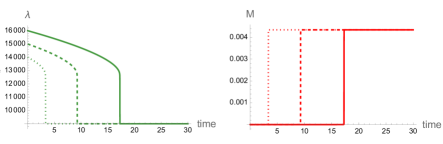
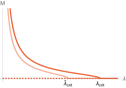
We conclude that this model exhibits a transcritical bifurcation with the property of having the zero trivial state stable for and replaced by a non-vanishing oligomer concentration for as shown in Figure 5. We observe that the critical clearance is independent of the saturation constant and that the asymptotic mass scales with that constant, giving the typical size allowable local oligomer load.
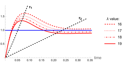
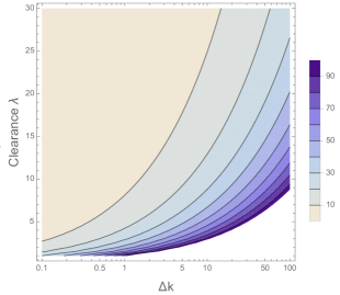
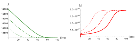
With the introduction of non-zero constant clearance in the system (13), there are now two timescales associated with the dynamics: a period of growth up to the maximum toxic mass at time where is the first eigenvalue of the system (13) when linearized, and a period of decay to time when where (Figure 5). Characteristic time scales for the amplification of the aggregate mass are obtained numerically and displayed in Figure 6. The impact of varying and on can also be seen by (14). The dependencies of both timescales on clearance and secondary nucleation are similar. Specifically, we observe that the impact of varying clearance on the timescales and toxic load in the system is profound.
Following the lag period, toxic mass is dominated by elongation and secondary nucleation, up to time when the dampening effects of clearance and saturation of secondary nucleation begin to dominate, initiating a decline in toxic mass from to the steady state . The peak toxic mass , fixed point , and associated timescales and , decrease with increased clearance. Increased secondary nucleation rates has an effect of increasing and and decreasing and , as expected from (14). Unless is altered dramatically, lowered by one order of magnitude, it has a marginal effect on lowering and with more effects in lowering and .
Increasing clearance has a more significant impact on decreasing toxic load in the local brain system (11) and both timescales and , and thus dominates in the preferential dampening effects at each phase of the disease cascade. Note that this model does not capture the full disease timescales in a human brain; transport and dynamic clearance have significant effects, as incorporated in the following sections.
If a steady state for exists (i.e. if is below some critical clearance threshold and is bounded), setting (11c) to zero, it must satisfy the recurrence relation
| (16) |
where each recursive effect is dependent on . Consequently, the fixed point of the -mer is
| (17) |
By definition,
| (18) |
where we define . Using this in solving (11b), we obtain
| (19) |
Thus, a fixed point exists if the following three conditions are satisfied:
| (20) | ||||
| (21) | ||||
| (22) |
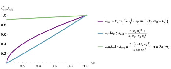
where (C1) reflects that the final concentration of aggregates must be decreasing with , (C2) must be bounded, and (C3) requires . Following methods presented in [49] we obtain the following analytical critical clearance formulae dependent on the form of clearance. This case is particularly interesting since, in the derivation of steady states, we see that a critical clearance can be established for different forms of size-dependent clearance. Remarkably, our results suggest that, depending on the specific size dependence, the processes of elongation and secondary nucleation contribute to the value of the critical clearance to different degrees. An important implication is that, depending on the specific mechanism of clearance, inhibition of aggregation should target different processes to reduce the critical clearance rate.
First considering constant clearance, as in (15), (C1–C3) are satisfied for
| (23) |
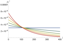
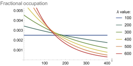
The size distribution for aggregates at equilibrium for varying subcritical constant clearance rates reveals that the relative occupation of oligomers in the region appears invariant to clearance. Increasing clearance uniformly in the constant clearance regime targets larger aggregates as seen in Figure 7. This is consistent with Oosawa theory [52, 53], which predicts that the length distribution initially develops into a Poisson distribution in the time taken for the monomer-polymer equilibrium to be established before relaxing over a longer time scale into an exponential distribution [43, Figure 5]. Due to the constant supply of monomers, oligomer concentrations are relatively higher, reflective of a brain region.
Considering size-dependent clearance , the infinite system (11) does not yield a closed system for the moments. Still, the fixed point solution (16) enables us to determine steady states for aggregate concentrations, subject to conditions for the existence of such a steady state (C1)-(C3). These existence conditions also facilitate the identification of the bifurcation point in clearance, , above which aggregation is negligible.
First, consider clearance that increases with aggregate size, . The biological understanding of this case might correspond to clearance mediated by drugs with preferential binding towards larger aggregates. In this case,
| (24) |
Since is increasing with aggregate size like , this intuitively suggests that a lower is required to avoid a diseased state.
For comparison, we consider the opposite case where clearance decreases with aggregate size with the biological interpretation that aggregates become more difficult to clear as they increase in size. Then, an analysis of (C1)-(C3) reveal a critical clearance of
| (25) |
which can be further simplified by again noting that , so we obtain the approximation .
2.3 A local model including aging and damage
As the mass of toxic proteins increases, it induces local damage that affects the proper function of the vasculature and all clearance mechanisms [54, 55, 56, 57]. To capture these effects, we let the clearance rates evolve in time up to a lower minimal clearance . The full system of equations now reads
| (26a) | |||
| (26b) | |||
| (26c) | |||
| (26d) | |||
with moment equations given by
| (27a) | ||||
| (27b) | ||||
All variables and parameters are given in Table 1, and we henceforth consider the value and form of . The dynamics of this system also display a bifurcation and requires sufficient seeding before it bifurcates to a non-trivial solution where as explained in [36].


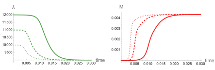

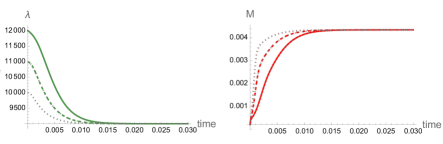

If we remove clearance in this model, it becomes equivalent to the previous (constant clearance) system (11) leading to unbounded growth. Once clearance decays to the basal clearance capacity associated with maximal damage, the dynamics of the system align with those of (11). However, the system dynamics prior to the point at which are markedly different, as we observe sigmoidal growth in toxic mass as local clearance is driven to the basal clearance capacity.
2.4 Coupling the microscopic model to transport
So far, we have developed a model suitable to describe the dynamics of oligomer concentrations within a single region. Next, we consider a system with multiple regions of interest connected through a network with diffusive transport between different regions. The brain connectome is defined as a weighted graph with nodes ( for vertices) and edges obtained from tractography of diffusion tensor images. From the tractography, we extract the weighted adjacency matrix and define the graph Laplacian
| (28) |
There are other possible definitions of the graph Laplacian obtained by normalizing rows, columns, or both. However, this is the only graph Laplacian that has the property preserves mass during transport and the requirement that no transport takes place between two regions with the same concentration (for a detailed description and discussion see [58]).
Incorporating the assumptions specified in the previous section, to approximate the seeded system, the truncated master equations for aggregates of size at node , including axonal transport, form an infinite system of first order ODES:
| (29a) | |||
| (29b) | |||
| (29c) | |||
| (29d) | |||
with initial conditions
| (30) |
Here is the diffusion coefficient of the -mer taken to be small or a function of [35, 59]. As before, the first two moments of the population distribution are
| (31) |
representing the total number and total mass concentrations of aggregates in the ROI , respectively. Taking clearance to be constant in time, the moment equations are given by:
| (32) | |||
| (33) |
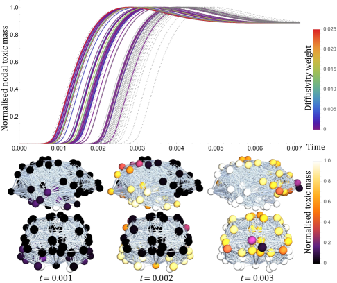
The order of node invasion across the brain network suggests a direct applicability of the diagonalization results of [35] to our model. In Figure 9, we observe immediate neighbors of the single seed node are invaded first, influenced heavily by the diffusivity weighting along the edges emanating from this seed. Subsequently, nodes of path length two are invaded, encompassing all nodes in the small-world network. Nodes with the lowest connectivity, such as the frontal pole, are invaded last. Figure 9 also displays the order of ROI invasion across the connectome and the corresponding network representation.
The growth of toxic mass across the connectome in this order is facilitated primarily by the transport of nuclei. To demonstrate this, first the distribution of oligomers of size 2, 4, 6 and 8, at a fixed time point, is seen in Figure 10 (first row) given a size-independent diffusion coefficient in (29). Aggregates spreading in travelling waves, and total toxic mass is a propagating front as described in [60]. It is observed experimentally [61, 62, 63] that in vivo aggregate transport scales with size. Specifically, large fibril assemblies do not move, and in previous models [59, 64] the diffusion coefficient of a soluble peptide is taken to scale as a reciprocal of the cube of its molecular weight.
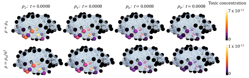
Perhaps counter-intuitively, the distinction in progression through nodes being characterised by first low weight oligomers, and later by increasing aggregate sizes, is not exacerbated by the assumption of transport scaling with size, as seen by comparing rows in Figure 10. The order of invasion and relative times of invasion remain the same, but the time taken to reach higher concentrations increases. This emphasises the role of nuclei spreading through the connectome, since local dynamics dominate over the delivery of aggregates by diffusion. We conclude that regardless of the form of size-dependent diffusivity, provided diffusion is small, the transport of larger aggregates does not significantly change the brain-wide dynamics.
3 Applications to therapeutic modelling
Next, we investigate the impact of monoclonal antibodies (mAbs), a form of immunotherapy known to influence microscopic parameters in chemical kinetic models, on the aggregation and propagation of misfolded toxic proteins. Using the local and brain scale models derived and studied in the previous section, we analyse, replicate, and propose treatment strategies on the structural connectome based on results in vitro. Parameters extracted in vitro are scaled up to display the impacts on whole-brain neurodegeneration to simulate treatments in a fully mechanistic model at the whole-brain scale. Notably, FDA-approved drugs such as lecanemab, and drugs with promising phase III trial results, such as donanemab, operate by ultimately increasing the effectiveness of brain clearance. Thus, a model that captures the intricacies of the brain’s endogenous clearance and the enhancement of this mechanism from drugs is crucial.
Linse et al. (2020) [25] found, by fixed point solution method of the coarse-grained protein kinetic equations, the kinetic fingerprints of various mAbs. For example, using the method described in [65], they identified that aducanumab causes an apparent reduction of the free oligomer concentration by inhibiting the critical molecular process, secondary nucleation, through which oligomers form. With the highest dose of aducanumab (100 nM), corresponding to a substoichiometric molar ratio of 0.03:1 antibody: A, there is a 69% reduction in the secondary nucleation rate constant. With the lowest dose tested (250 pM), there is still a 39% reduction. Thus one effect of the drug on the aggregation pathway can be expressed as a rate constant change in the presence of aducanumab:
| (34) |
where is dependent on the dose of the drug. Importantly, variations in reduce the critical clearance for all models, as seen in Figure 11, with implications for disease timescales and propagation patterns as discussed in [36].
The inhibitory effect on secondary nucleation originates from the interaction of aducanumab with amyloid fibrils. Linse et al. (2020) [25] observed a low affinity for monomers and a very high affinity (1nM) for fibrils, in agreement with previous findings [66]. Fibrils become fully coated with aducanumab along their entire length, effectively interfering with secondary nucleation at the fibril surface. Further, mAbs binding to amyloid fibrils targets them for microglia-mediated removal and enhances the clearance of plaques [67, 68].
Mazer et al. (2023) [37] model the effect of drugs solely through increased clearance in a compartmental model; the Q-ATN model. The pharmacodynamic (PD) drug effect of antibody-mediated plaque removal is quantified by a linear relationship between antibody concentration and clearance. The PD model assumes a pseudo-first-order rate constant for plaque removal () that is proportional to the plasma concentration (), with an antibody-specific proportionality constant () given by
| (35) |
The values were estimated by fitting the time course of mean amyloid PET data during treatment using a non-linear least squares algorithm.
We directly substitute drug inhibited parameters into the system (11) to obtain, in the case of aducanumab,
| (36a) | |||
| (36b) | |||
| (36c) | |||
where, as before,
| (37) |
Next, we consider the effects of aducanumab on only the kinetic parameters expressed through the reduced secondary nucleation rate constant , identified to be the drug’s inhibitory action on the aggregation chain. This results in a new critical clearance, which varies with according to (15) (Figure 11), and the steepness of the fixed state according to (14). The toxic mass equilibrium is shown in Figure 12 in the presence of the kinetic action of aducanumab (orange) and without treatment (red). In addition to this kinetic effect, [37] suggest that the preferential binding of aducanumab to fibrils facilitates clearance at a rate proportional to drug concentration. Therefore, we model this effect by increasing aggregate size-specific clearance by .
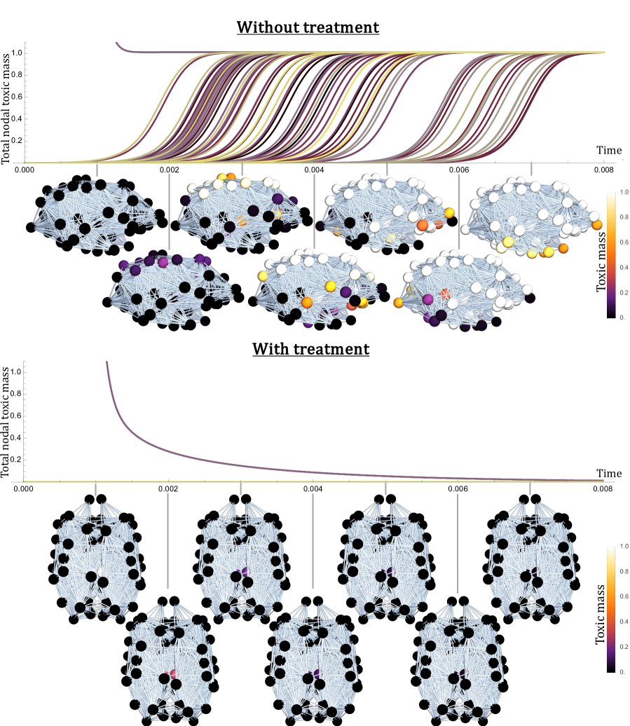
Next, we couple (36) to transport across the connectome using the graph Laplacian, as done in (29). In the growth-dominated regime, the homogeneous system is a good approximation of the brain-scale system. The progression throughout the brain network, with and without treatment, is illustrated in Figure 13 for A, considering an initial clearance of in the network aggregation-clearance model (29). This brain-wide drug simulation highlights the capability of monoclonal antibodies to localise the disease if caught within the clearance window of . This dependence on drug efficacy on initial clearance, along with the characterisation of the drugs effects purely in terms of brain clearance, further emphasises the pivotal role of clearance in neurodegeneration.
4 Mathematically informed treatment strategies
Mathematical models provide a platform for experiments that would be otherwise difficult or impossible to conduct in humans. Here we study potential treatment strategies based on our network model of brain-scale aggregation with in vivo effects.
4.1 Target clearance of smaller aggregates
Different drugs target aggregates of different sizes. We simulate this effect by assuming that clearance halts or reduces neurodegeneration. An enhanced clearance , will specifically affect aggregates within a particular size interval, in addition to the natural (assumed to be initially subcritical) background clearance of the human brain. To capture these effects in a local model representative of a single brain region in vivo like (11), we keep the clearance rates constant for most sizes but elevated dramatically across an interval :
| (38a) | |||
| (38b) | |||
| (38c) | |||
| (38d) | |||
where
| (39) |
with the corresponding reduced moments system
| (40a) | |||
| (40b) | |||
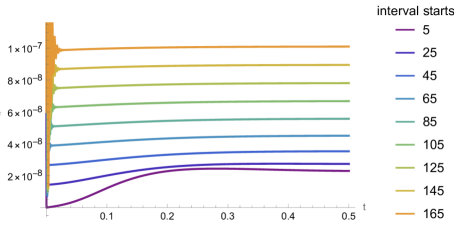
As seen in Figure 14, we perform a sweep of intervals and observe that targeting aggregates of smaller size decreases the total toxic mass in the system the most. This underscores the fundamental role of secondary nucleation in forming plaques and indicates that smaller aggregates constitute the largest toxic mass in the system.
An explanation of the observed results in Figure 14 can be understood by considering the fixed point solutions. Specifically, a steady state for satisfies the recurrence relation
| (41) |
where each recursive effect is dependent on . Consequently, the fixed point of the -mer is
| (42) |
Removing -mers of sizes gives the toxic mass fixed point,
| (43) |
where we define , and
| (44) |
It remains to prove that
| (45) |
or
| (46) |
for where . Expanding the brackets, to leading order
| (47) |
where . Since there is a fixed difference between intervals, say ,
| (48) |
so we require
| (49) |
Further, there is also a fixed interval size so
| (50) |
that is,
| (51) |
which holds true since . Hence, in the constant clearance regime, removing intervals of smaller aggregates reduces the total toxic mass equilibrium more than removing the same-sized intervals of larger aggregates. It remains to explore the effect of removing larger intervals of larger aggregates and a critical interval size, which would be more valuable than removing lower-weight oligomers.
Given the pronounced toxicity of oligomeric intermediates relative to larger fibrillar species, actively eliminating oligomers has a dual impact. By targeting smaller aggregates, we significantly reduce the total toxic mass to the greatest extent possible. This approach aligns with our primary objective of addressing the most toxic species generated during aggregation. As a reference, aducanumab partially targets oligomers but mostly clears insoluble amyloid plaques [69].
4.2 Optimal drug administration strategies
A variety of dosing strategies can be analysed and simulated directed in the nucleation-aggregation-clearance model with in vivo effects (11). In this section, we formulate an optimisation problem with the objective of minimising the accumulation of toxic mass in a given time period, over the parameters of the functional form of drug-induced clearance . This allows us to determine the optimal frequency and volume of doses, while adhering to drug toxicity constraints, in the context of a computational drug trial.
Assuming a linear relationship between antibody concentration and clearance as proposed by [37], we take the concentration of the drug administered to be directly proportional to the drug-enhanced clearance increment . That is, where is drug concentration and is constant. In the first instance, we assume that drug administration is spaced equally and decays exponentially, being cleared from the brain as a non-aggregating particle. Emulating the drug concentration profiles described in [37, Figure 1], we simulate a dosing regime through the following clearance profile:
| (52) |
in (11). Here is the clearance rate of the drug from the brain, is the time period (days) between drug doses, is the background natural clearance, and is the drug-enhanced increase in clearance that is assumed to be proportional to the dose.
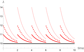
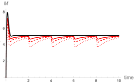
To demonstrate the effects of this dosing regime, clearance profiles (52) and the response in toxic mass evolution according to (11) are displayed in Figure 15 corresponding to three dosing strategies. In this example, for illustrative purposes, the black curves show the no-treatment case, and only (the dosage) varies across strategies with fixed , , and ambient clearance . We observe a sinusoidal steady state in the presence of drugs, with the steady state’s peak reducing and the steady state’s range increasing, with increasing.

Considering the effects of varying both and on misfolded protein mass, herein referred to as the regime parameters, the best strategy is to maximise the frequency and volume of treatments. However, there is a cost involved in raising (dosage) and reducing (time between each dose) due to the toxicity of antibodies to the brain environment, such as a significant risk of amyloid-related imaging abnormality (ARIA) [70, 71]. With this in mind, the following optimisation problem naturally arises.
Given a trial period of say days, we aim to identify the optimal number of days between drug administration and volume of drugs given that is proportional to drug-induced clearance . We supplement the problem with the constraint that the total mass of drugs (mg) administered during this period invokes a limited integrated clearance increment, denoted . For simplicity, we choose , assuming that remains constant as clearance increases. We optimise and such that the average toxic mass across one cycle of drug administration, i.e. the average of the steady states shown in Figure 15(b), , is minimised. In full, the optimisation problem reads
| (53) | |||
| subject to | (54) | ||
| (55) |
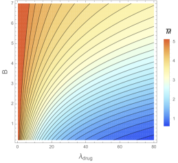
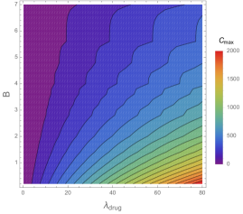
Contour plots of the average toxic mass for varying regime parameters are shown in Figure 16(a), with the corresponding drug toxicity shown in Figure 16(b). We identify the optimal dosing regime, subject to a specific drug toxicity constraint by consulting the combination of Figure 16(a) and (b) in Figure 17. Solutions satisfying the constraints in (55) lie along the respective dashed lines, and the colour function displays the relative average toxic mass equilibrium . Subject to these constraints, solutions with the lowest average toxic mass correspond to the lowest spacing between doses, .
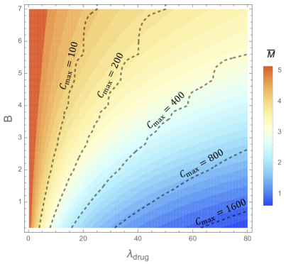
The optimal strategy, therefore, is the trivial one: to take , corresponding to a constant supply of drugs. Of course, this could be impractical or detrimental to a patient’s quality of life. Given the potential impracticality of constant drug supply, the key question is at what cost, in terms of toxic mass , can drug doses be distributed (increasing ). For reference, consider regime parameters corresponding to in (55). The optimal solution, a constant supply of drugs with , results in the minimum allowable average toxic mass of . Other solutions satisfying the same drug toxicity constraint, but not necessarily minimising , are shown in Figure 17 and demonstrate some flexibility in dosing strategies. For example, once a day results in the only slightly increased . A solution with seven days between doses of results in a similar average toxic steady state of , albeit with a higher variance around this equilibrium. This implies some leniency on dosing frequency. Overall, as seen in Figure 17, does not greatly vary along the constant contours; the contours of and in Figure 16(a) and (b) follow similar trends. The amount that varies with with constant is dependent on , as observed by the higher range in values along the contour compared to the contour. Therefore, depending on and the desired reduction in toxic mass, increasing the days between doses can lead to insignificant increases in toxic mass, with potentially significant improvements in quality of life.
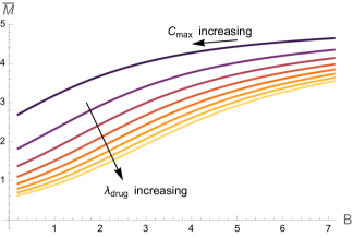
In addition, as shown by Figure 18, keeping constant and lowering can have a high impact on reducing for smaller values of but is less impactful for higher . Further, increasing is less impactful for higher values of (shown by the lighter curves). Together, these results hold potential in determining dosing strategies in personalised medicine, with initial conditions of (11) reflecting the initial toxic loads of patients and parameters in (52) tunable to the desired reduction in toxic load.
5 Discussion
Theoretical research into toxic mass accumulation in neurodegenerative diseases has thus far exclusively consisted of either detailed in vitro analysis of aggregation kinetics or in vivo studies on the effects of transport and clearance in macroscale models on networks, with the former being validated against experimental observations and the latter with structural data. Both aspects have proved essential for our understanding of AD pathology. However, there is a cloudy middle ground restricting our understanding of aggregation inside the complex domain of the human brain. The development of a nucleation-aggregation model which includes in vivo effects such as protein production, saturation, transport and, most importantly, the clearance of solutes, remains a task that has only been addressed mechanistically in two prior studies [35, 49]. Fornari et al. (2019) [35] used a Smoluchowski-type model to analyse the effect of aggregate transport at the brain scale, while Thompson et al. (2021) [49] considered the effects of a bulk constant clearance at the microscopic scale. Our work combines both approaches within the same mathematical framework, establishing a general picture for the self-assembly of A in the aggregation cascade in vivo across the connectome. We have derived a class of nucleation-aggregation-clearance models for the homogeneous dynamics and spatial progression of A in the brain, tracking the evolution of different size aggregates with distinct properties instrumental in neurodegeneration. This new class of models provides a therapeutic modelling platform reflective of the human brain for the simulation of potential therapies at the spatial and temporal scales of the disease. Notably, we reveal the therapeutic effect of enhanced clearance behind the success of recent drug trials. The dependence of drug efficacy on initial clearance, along with the characterisation of the drug’s effects purely in terms of clearance, further emphasises the pivotal role of clearance in neurodegeneration.
5.1 Brain scale models of nucleation, aggregation, clearance and transport
The first primary aim of this work was to develop a comprehensive and entirely mechanistic model encompassing the aforementioned in vivo effects, along with physiological effects not previously modeled, with a focus on quantifying the role of dynamic clearance of aggregates in neurodegeneration at the brain scale. To address the complexities of developing a model representative of a single brain region, we advance current state-of-the-art chemical kinetic models by incorporating physiological effects observed in experiments. Then, we include strong transport anisotropy in the brain through the graph Laplacian to simulate aggregate dynamics across the spectrum of aggregate sizes at the brain scale. The study of such systems is guided by the homogeneous case for which both total mass evolution and aggregates’ size distribution are obtained analytically, and bifurcation analysis reveals critical clearance regimes dependent on kinetic rate constants.
At the local ROI level, analysis of the homogeneous nucleation-aggregation-clearance models (11) reveals that the clearance rate dictates the timescale of the nucleated transition to an aggregated brain region and the final toxic mass equilibrium. In the absence of a simulated seed, an increase in toxic mass is characterised by an early phase of seeding depending on primary nucleation, followed by a period of linear growth mostly controlled by aggregation of monomers onto the fibril, and then a phase of autocatalytic growth dominated by the multiplicative processes of secondary nucleation and elongation. Once enough toxic mass accumulates, clearance dominates, and the toxic mass approaches a saturated steady state. Importantly the critical clearance rate, above which all aggregates clear from a brain region, holds significant therapeutic potential. Recovering similar results to [49], the critical clearance formulae depend upon the assumed clearance form relative to aggregate size, with different dependencies on the aggregation rate constants. When analysing the local system with dynamic clearance given by (26), local clearance reduces to the basal clearance capacity at rates relative to the difference between initial clearance and basal clearance. After this point the dynamics of the system are equivalent to those of the homogeneous nucleation-aggregation-clearance models (11) so we recover the same critical basal clearance regimes as for clearance in (11).
To model the interplay between aggregation and clearance at the brain-scale, the local dynamics are coupled with anisotropic transport across the connectome in (29). As identified first by [35], the progression of the disease consists of an initial stage that develops at the seeded node, followed by primary infection in connected nodes, mainly driven by diffusion rather than aggregation kinetics. These nodes distribute seeds, and due to the brain’s small-world network structure, secondary infection develops in most nodes soon after primary infection. In the growth-dominated regime representative of the toxic protein cascade in a human brain, local dynamics dominate once a node receives a seed by primary or secondary infection. We thus find that the analytical results of the homogeneous model (11) are a good approximation for the connected dynamics at the brain scale. Furthermore, the brain-scale dynamics appear invariant to the diffusion of aggregates larger than nuclei, indicating that the transport of dimers is the primary factor driving pathology, and size-dependent diffusion does not significantly alter the dynamics.
5.2 Therapeutic modelling insights
The pivotal field of Alzheimer’s drug design commands extensive research activity. Yet, drug trials and drug performance projections rely on data without providing comprehensive insights into the mechanisms of drug action. Current microscopic chemical kinetic models shed light on how drugs influence the aggregation process [25], while empirical compartmental models project the longer-term effects of anti-amyloid treatments by fitting data from clinical trials to semi-mechanistic macroscale models [37], with no consideration of the drug action at the microscale. Our in vivo nucleation-aggregation-clearance model aims to bridge the gap between these two approaches, extending in vitro observations to decades of AD pathology at the brain scale, considering both the increase in clearance due to drugs and the inhibition of specific steps in the aggregation process. We thus present the first fully mechanistic model of brain-scale in vivo aggregation growth, clearance and transport that can describe the effects of therapeutic agents both analytically and through direct simulation, aid drug performance projection, and lead exploratory theoretical studies to ultimately guide drug design. We thus quantified the action of potential drugs on protein aggregation in vivo, and conducted a preliminary study on the most favorable treatment strategies, concerning optimal aggregate sizes to target, specific microscopic steps of aggregation to inhibit, and the frequency and volume of antibody dosage.
Specifically, we modeled the mechanism of action of treatments in the homogeneous system (36) and its corresponding brain-scale extensions to see the effect of the antibodies on the disease dynamics. For aducanumab, we modeled the pharmacodynamic property of a decreased secondary nucleation rate constant due to the drug binding to fibrils, thus inhibiting the aggregation process [25] and mediating enhanced clearance, as considered by [37]. First focusing solely on the kinetic drug effects we observe a consistent pattern across all models: a decrease in critical clearance, leading to an improvement in the effectiveness of compromised local clearance. This enables a patient under treatment to completely transition to a healthy state or experience a lessened toxic load, depending on the initial clearance at the time of commencing therapy. Mathematically, the inhibitory actions of potential therapeutic agents on the aggregation process transforms the aggregated equilibrium (Figure 12). Thus through steady-state analysis, we identify that the primary therapeutic effect of the drugs is a reduction in critical clearance, increasing the system’s overall effective clearance.
Considering the drug’s effect in the microscopic aggregation model (36) coupled to transport allows us to track the response in the evolution of distinct aggregate sizes across the connectome. The effects of the kinetic action of treatment are the same: a transformation of the toxic steady-state solution in the presence of drugs (Figure 12), with the potential to initiate a transition from an unhealthy patient state () to a healthy state () in which the otherwise compromised clearance rates are sufficient to completely remove toxic mass in the presence of drugs. The complete inhibition of aggregation and propagation shown in Figure 13 is due only to the kinetic action of the drug reducing increasing the effectiveness of the brains damaged clearance mechanisms. This transition from an unhealthy state to a healthy equilibrium is dependent upon the brain’s initial clearance upon drug administration, underscoring the need for treatments early on in disease progression when . The impact of drugs such as aducanumab on secondary nucleation thus has a profound effect, employing a decrease in the aggregation kinetic rate constants thereby improving the effectiveness of brain clearance. Our most critical finding is that the drug’s kinetic effect alone can be sufficient for a transition from a brain with detrimental levels of toxic mass to a healthy state. In addition, considering enhanced clearance due to drug binding in combination with the kinetic effect of the drugs leads to a more pronounced reduction in long-term toxic mass accumulation. Significantly, in the presence of drugs, the critical toxic seed as discussed in [36] is increased, so it is less likely that a dynamic clearance will drop below critical.
Ultimately, our brain-scale nucleation-aggregation-clearance models open up avenues for the mathematically-informed therapeutic strategies to control pathological protein aggregation, addressing questions that current modelling studies fail to address at the brain scale. We have identified that a reduction in is successful in curing patients. Quantifying the actions of drugs in this way allows us to identify which rate constants might inhibit aggregation to provide the largest reduction in . For example, if considering the size dependant clearance to be reflective of the human body, the form of the critical clearance rate (25) suggests that targeting the elongation processes would be most effective in reducing the critical clearance and most vitally translating the fixed point solution curve. Further, we performed a sweep of an interval of increased clearance and uncovered that targeting smaller aggregates is more impactful than targeting larger ones. Additionally, we studied an optimization problem to demonstrate how the models can inform dosing regimens, as described and simulated in [37]. The results suggest that more frequent dosing is preferable for reducing average toxic mass and variance, although combinations of higher, less frequent doses can achieve the same steady states. A more in-depth analysis of the application of these models for pharmacological use is of great interest for future studies.
Acknowledgements
The work of A.G. was supported by the Engineering and Physical Sciences Research Council under Research grant EP/R020205/1. This publication is based on work supported by the EPSRC Centre For Doctoral Training in Industrially Focused Mathematical Modelling (EP/L015803/1) in collaboration with Simula Research Laboratory. For the purpose of Open Access, the authors will apply a CC BY public copyright license to any Author Accepted Manuscript (AAM) version arising from this submission. The help of Travis Thompson and Hadrien Oliveri with numerical and conceptual issues is gratefully acknowledged.
Data Availability
The manuscript has no associated data.
References
- [1] D. M. Fowler, A. V. Koulov, C. Alory-Jost, M. S. Marks, W. E. Balch, and J. W. Kelly. Functional amyloid formation within mammalian tissue. PLoS Biology, 4(1):e6, 2006.
- [2] S. K. Maji, M. H. Perrin, M. R. Sawaya, S. Jessberger, K. Vadodaria, R. A. Rissman, P. S. Singru, K. P. R. Nilsson, R. Simon, D. Schubert, et al. Functional amyloids as natural storage of peptide hormones in pituitary secretory granules. Science, 325(5938):328–332, 2009.
- [3] A. Bleem and V. Daggett. Structural and functional diversity among amyloid proteins: agents of disease, building blocks of biology, and implications for molecular engineering. Biotechnology and Bioengineering, 114(1):7–20, 2017.
- [4] T. P. J. Knowles and R. Mezzenga. Amyloid fibrils as building blocks for natural and artificial functional materials. Advanced Materials, 28(31):6546–6561, 2016.
- [5] F. Chiti and C. M. Dobson. Protein misfolding, functional amyloid, and human disease. Annual Review of Biochemistry, 75:333–366, 2006.
- [6] F. Chiti and C. M. Dobson. Protein misfolding, amyloid formation, and human disease: a summary of progress over the last decade. Annual Review of Biochemistry, 86:27–68, 2017.
- [7] T. P. J. Knowles, M. Vendruscolo, and C. M. Dobson. The amyloid state and its association with protein misfolding diseases. Nature Reviews Molecular Cell Biology, 15(6):384–396, 2014.
- [8] M. Wortmann. Dementia: a global health priority-highlights from an ADI and World Health Organization report. Alzheimer’s Research & Therapy, 4:1–3, 2012.
- [9] P. T. Lansbury. A reductionist view of Alzheimer’s disease. Accounts of Chemical Research, 29(7):317–321, 1996.
- [10] M. Goedert, M. Masuda-Suzukake, and B. Falcon. Like prions: the propagation of aggregated tau and -synuclein in neurodegeneration. Brain, 140(2):266–278, 2017.
- [11] B. Frost and M. I. Diamond. Prion-like mechanisms in neurodegenerative diseases. Nature Reviews Neuroscience, 11(3):155–159, 2010.
- [12] M. Jucker and L. C. Walker. Propagation and spread of pathogenic protein assemblies in neurodegenerative diseases. Nature Neuroscience, 21(10):1341–1349, 2018.
- [13] T. T. Olsson, O. Klementieva, and G. K. Gouras. Prion-like seeding and nucleation of intracellular amyloid-\textbeta. Neurobiology of Disease, 113:1–10, 2018.
- [14] M. Goedert. Alzheimer’s and Parkinson’s diseases: The prion concept in relation to assembled A\textbeta, tau, and \textalpha-synuclein. Science, 349(6248):1255555, 2015.
- [15] A. Mudher, M. Colin, S. Dujardin, M. Medina, I. Dewachter, S. M. A. Naini, E.-M. Mandelkow, E. Mandelkow, L. Buée, M. Goedert, et al. What is the evidence that tau pathology spreads through prion-like propagation? Acta Neuropathologica Communications, 5(1):99, 2017.
- [16] S. B. Prusiner. Prions. Proceedings of the National Academy of Sciences, 95(23):13363–13383, 1998.
- [17] J. A. Hardy and G. A. Higgins. Alzheimer’s disease: the amyloid cascade hypothesis. Science, 256(5054):184–186, 1992.
- [18] J. Hardy and D. Allsop. Amyloid deposition as the central event in the aetiology of Alzheimer’s disease. Trends in Pharmacological Sciences, 12:383–388, 1991.
- [19] D. J. Selkoe and J. Hardy. The amyloid hypothesis of Alzheimer’s disease at 25 years. EMBO Molecular Medicine, 8(6):595–608, 2016.
- [20] D. J. Selkoe. Alzheimer’s disease: genes, proteins, and therapy. Physiological Reviews, 2001.
- [21] T. Härd and C. Lendel. Inhibition of amyloid formation. Journal of Molecular Biology, 421(4-5):441–465, 2012.
- [22] E. Karran and B. De Strooper. The amyloid hypothesis in Alzheimer disease: new insights from new therapeutics. Nature Reviews Drug Discovery, 21(4):306–318, 2022.
- [23] W. Hong, Z. Wang, W. Liu, T. T. O’Malley, M. Jin, M. Willem, C. Haass, M. P. Frosch, and D. M. Walsh. Diffusible, highly bioactive oligomers represent a critical minority of soluble A in Alzheimer’s disease brain. Acta Neuropathologica, 136:19–40, 2018.
- [24] D. M. Walsh and D. J. Selkoe. Amyloid -protein and beyond: The path forward in Alzheimer’s disease. Current Opinion in Neurobiology, 61:116–124, 2020.
- [25] S. Linse, T. Scheidt, K. Bernfur, M. Vendruscolo, C. M. Dobson, S. I. A. Cohen, E. Sileikis, M. Lundqvist, F. Qian, T. O’Malley, et al. Kinetic fingerprints differentiate the mechanisms of action of anti-A antibodies. Nature Structural & Molecular Biology, 27(12):1125–1133, 2020.
- [26] B. Rumble, R. Retallack, C. Hilbich, G. Simms, G. Multhaup, R. Martins, A. Hockey, P. Montgomery, K. Beyreuther, and C. L. Masters. Amyloid A4 protein and its precursor in Down’s syndrome and Alzheimer’s disease. The New England Journal of Medicine, 320(22):1446–1452, 1989.
- [27] A. Bacyinski, M. Xu, W. Wang, and J. Hu. The paravascular pathway for brain waste clearance: current understanding, significance and controversy. Frontiers in Neuroanatomy, 11:101, 2017.
- [28] J. M. Tarasoff-Conway, R. O. Carare, R. S. Osorio, L. Glodzik, T. Butler, E. Fieremans, L. Axel, H. Rusinek, C. Nicholson, B. V. Zlokovic, et al. Clearance systems in the brain - implications for Alzheimer disease. Nature Reviews Neurology, 11(8):457–470, 2015.
- [29] S.-H. Xin, L. Tan, X. Cao, J.-T. Yu, and L. Tan. Clearance of amyloid beta and tau in Alzheimer’s disease: from mechanisms to therapy. Neurotoxicity Research, 34:733–748, 2018.
- [30] M. Dobson. The Story of Medicine. Quercus Books, 2013.
- [31] G. Klein, P. Delmar, N. Voyle, S. Rehal, C. Hofmann, D. Abi-Saab, M. Andjelkovic, S. Ristic, G. Wang, R. Bateman, et al. Gantenerumab reduces amyloid- plaques in patients with prodromal to moderate Alzheimer’s disease: a PET substudy interim analysis. Alzheimer’s Research & Therapy, 11(1):1–12, 2019.
- [32] M. Ten Kate, S. Ingala, A. J. Schwarz, N. C. Fox, G. Chételat, B. N. M. van Berckel, M. Ewers, C. Foley, J. D. Gispert, D. Hill, et al. Secondary prevention of Alzheimer’s dementia: neuroimaging contributions. Alzheimer’s Research & Therapy, 10(1):1–21, 2018.
- [33] L. C. Walker and M. Jucker. Neurodegenerative diseases: expanding the prion concept. Annual Review of Neuroscience, 38:87–103, 2015.
- [34] S. Fornari, A. Schäfer, M. Jucker, A. Goriely, and E. Kuhl. Prion-like spreading of Alzheimer’s disease within the brain’s connectome. Journal of the Royal Society Interface, 16(159):20190356, 2019.
- [35] S. Fornari, A. Schäfer, E. Kuhl, and A. Goriely. Spatially-extended nucleation-aggregation-fragmentation models for the dynamics of prion-like neurodegenerative protein-spreading in the brain and its connectome. Journal of Theoretical Biology, 486:110102, 2020.
- [36] G. S. Brennan, T. B. Thompson, H. Oliveri, M. E. Rognes, and A. Goriely. The role of clearance in neurodegenerative diseases. SIAM Journal on Applied Mathematics, pages S172–S198, 2023.
- [37] N. A. Mazer, C. Hofmann, D. Lott, R. Gieschke, G. Klein, F. Boess, H. P. Grimm, G. A. Kerchner, M. Baudler-Klein, J. Smith, et al. Development of a quantitative semi-mechanistic model of Alzheimer’s disease based on the amyloid/tau/neurodegeneration framework (the Q-ATN model). Alzheimer’s & Dementia, 19(6):2287–2297, 2023.
- [38] G. Meisl, L. Rajah, S. A. I. Cohen, M. Pfammatter, A. Šarić, E. Hellstrand, A. K. Buell, A. Aguzzi, S. Linse, M. Vendruscolo, et al. Scaling behaviour and rate-determining steps in filamentous self-assembly. Chemical Science, 8(10):7087–7097, 2017.
- [39] R. Frankel, M. Törnquist, G. Meisl, O. Hansson, U. Andreasson, H. Zetterberg, K. Blennow, B. Frohm, T. Cedervall, T. P. J. Knowles, et al. Autocatalytic amplification of Alzheimer-associated A42 peptide aggregation in human cerebrospinal fluid. Communications Biology, 2(1):365, 2019.
- [40] F. Kundel, L. Hong, B. Falcon, W. A. McEwan, T. C. T. Michaels, G. Meisl, N. Esteras, A. Y. Abramov, T. J. P. Knowles, M. Goedert, et al. Measurement of tau filament fragmentation provides insights into prion-like spreading. ACS Chemical Neuroscience, 9(6):1276–1282, 2018.
- [41] S. I. A. Cohen, M. Vendruscolo, M. E. Welland, C. M. Dobson, E. M. Terentjev, and T. P. J. Knowles. Nucleated polymerization with secondary pathways. I. Time evolution of the principal moments. The Journal of Chemical Physics, 135(6), 2011.
- [42] S. I. A. Cohen, M. Vendruscolo, C. M. Dobson, and T. P. J. Knowles. Nucleated polymerization with secondary pathways. II. Determination of self-consistent solutions to growth processes described by non-linear master equations. The Journal of Chemical Physics, 135(6), 2011.
- [43] S. I. A. Cohen, M. Vendruscolo, C. M. Dobson, and T. P. J. Knowles. Nucleated polymerization with secondary pathways. III. Equilibrium behavior and oligomer populations. The Journal of Chemical Physics, 135(6), 2011.
- [44] G. Meisl, X. Yang, B. Frohm, T. P. J. Knowles, and S. Linse. Quantitative analysis of intrinsic and extrinsic factors in the aggregation mechanism of alzheimer-associated A-peptide. Scientific Reports, 6(1):18728, 2016.
- [45] X. Yang, G. Meisl, B. Frohm, E. Thulin, T. P. J. Knowles, and S. Linse. On the role of sidechain size and charge in the aggregation of a 42 with familial mutations. Proceedings of the National Academy of Sciences, 115(26):E5849–E5858, 2018.
- [46] M. R. Nilsson, M. Driscoll, and D. P. Raleigh. Low levels of asparagine deamidation can have a dramatic effect on aggregation of amyloidogenic peptides: implications for the study of amyloid formation. Protein Science, 11(2):342–349, 2002.
- [47] M. Jucker and L. C. Walker. Pathogenic protein seeding in Alzheimer disease and other neurodegenerative disorders. Annals of Neurology, 70(4):532–540, 2011.
- [48] M. Jucker and L. C. Walker. Self-propagation of pathogenic protein aggregates in neurodegenerative diseases. Nature, 501(7465):45–51, 2013.
- [49] T. B. Thompson, G. Meisl, T. P. J. Knowles, and A. Goriely. The role of clearance mechanisms in the kinetics of pathological protein aggregation involved in neurodegenerative diseases. Journal of Chemical Physics, 154(12):125101, 2021.
- [50] G. Meisl, X. Yang, E. Hellstrand, B. Frohm, J. B. Kirkegaard, S. I. A. Cohen, C. M. Dobson, S. Linse, and T. P. J. Knowles. Differences in nucleation behavior underlie the contrasting aggregation kinetics of the A40 and A42 peptides. Proceedings of the National Academy of Sciences U.S.A., 111(26):9384–9389, 2014.
- [51] S. I. A. Cohen, S. Linse, L. M. Luheshi, E. Hellstrand, D. A. White, L. Rajah, D. E. Otzen, M. Vendruscolo, C. M. Dobson, and T. P. J. Knowles. Proliferation of amyloid-42 aggregates occurs through a secondary nucleation mechanism. Proceedings of the National Academy of Sciences, 110(24):9758–9763, 2013.
- [52] F. Oosawa and S. Asakura. Thermodynamics of the Polymerization of Protein. Academic Press, 1975.
- [53] F. Oosawa. Size distribution of protein polymers. Journal of Theoretical Biology, 27(1):69–86, 1970.
- [54] R. E. Bennett, A. B. Robbins, M. Hu, X. Cao, R. A. Betensky, T. Clark, S. Das, and B. T. Hyman. Tau induces blood vessel abnormalities and angiogenesis-related gene expression in P301L transgenic mice and human Alzheimer’s disease. Proceedings of the National Academy of Sciences, 115(6):E1289–E1298, 2018.
- [55] P. Carrillo-Mora, R. Luna, and L. Colin-Barenque. Amyloid beta: multiple mechanisms of toxicity and only some protective effects? Oxidative Medicine and Cellular Longevity, 2014:795375, 2014.
- [56] I. Canobbio, A. A. Abubaker, C. Visconte, M. Torti, and G. Pula. Role of amyloid peptides in vascular dysfunction and platelet dysregulation in Alzheimer’s disease. Frontiers in Cellular Neuroscience, 9:65, 2015.
- [57] A. Michalicova, P. Majerova, and A. Kovac. Tau protein and its role in blood–brain barrier dysfunction. Frontiers in Molecular Neuroscience, 13:570045, 2020.
- [58] G. S. Brennan and A. Goriely. An introduction to network models of neurodegenerative diseases. In J. Dokken, K.-A. Mardal, M. E. Rognes, L. M. Valnes, and V. Vinje, editors, Mathematical modeling of the human brain: from deep learning to glymphatics. Springer, 2025. (accepted).
- [59] M. Bertsch, B. Franchi, N. Marcello, M. C. Tesi, and A. Tosin. Alzheimer’s disease: a mathematical model for onset and progression. Mathematical Medicine and Biology: A Journal of the IMA, 34(2):193–214, 2017.
- [60] P. Putra, H. Oliveri, T. Thompson, and A. Goriely. Front propagation and arrival times in networks with application to neurodegenerative diseases. SIAM Journal on Applied Mathematics, 83(1):194–224, 2023.
- [61] C. Nicholson, K. C. Chen, S. Hrabětová, and L. Tao. Diffusion of molecules in brain extracellular space: theory and experiment. Progress in Brain Research, 125:129–154, 2000.
- [62] G. J. Goodhill. Diffusion in axon guidance. European Journal of Neuroscience, 9(7):1414–1421, 1997.
- [63] C. Nicholson and E. Syková. Extracellular space structure revealed by diffusion analysis. Trends in Neurosciences, 21(5):207–215, 1998.
- [64] Y. Achdou, B. Franchi, N. Marcello, and M. C. Tesi. A qualitative model for aggregation and diffusion of -amyloid in Alzheimer’s disease. Journal of Mathematical Biology, 67(6-7):1369–1392, 2013.
- [65] G. Meisl, J. B. Kirkegaard, P. Arosio, T. C. T. Michaels, M. Vendruscolo, C. M. Dobson, S. Linse, and T. P. J. Knowles. Molecular mechanisms of protein aggregation from global fitting of kinetic models. Nature Protocols, 11(2):252–272, 2016.
- [66] J. W. Arndt, F. Qian, B. A. Smith, C. Quan, K. P. Kilambi, M. W. Bush, T. Walz, R. B. Pepinsky, T. Bussière, S. Hamann, et al. Structural and kinetic basis for the selectivity of aducanumab for aggregated forms of amyloid-. Scientific Reports, 8(1):6412, 2018.
- [67] J. Sevigny, P. Chiao, T. Bussière, P. H. Weinreb, L. Williams, M. Maier, R. Dunstan, S. Salloway, T. Chen, Y. Ling, et al. The antibody aducanumab reduces A plaques in Alzheimer’s disease. Nature, 537(7618):50–56, 2016.
- [68] L. Söderberg, M. Johannesson, P. Nygren, H. Laudon, F. Eriksson, G. Osswald, C. Möller, and L. Lannfelt. Lecanemab, aducanumab, and gantenerumab— binding profiles to different forms of amyloid-beta might explain efficacy and side effects in clinical trials for Alzheimer’s disease. Neurotherapeutics, 20(1):195–206, 2023.
- [69] M. Tolar, S. Abushakra, J. A. Hey, A. Porsteinsson, and M. Sabbagh. Aducanumab, gantenerumab, BAN2401, and ALZ-801 — the first wave of amyloid-targeting drugs for Alzheimer’s disease with potential for near term approval. Alzheimer’s Research & Therapy, 12:1–10, 2020.
- [70] C. G. Withington and R. S. Turner. Amyloid-related imaging abnormalities with anti-amyloid antibodies for the treatment of dementia due to Alzheimer’s disease. Frontiers in Neurology, 13:862369, 2022.
- [71] J. Cummings, P. Aisen, L. G. Apostolova, A. Atri, S. Salloway, and M. Weiner. Aducanumab: appropriate use recommendations. The Journal of Prevention of Alzheimer’s Disease, 8:398–410, 2021.