Hybrid NOMA Assisted OFDMA Uplink Transmission

Abstract

Hybrid non-orthogonal multiple access (NOMA) has recently received significant research interest due to its ability to efficiently use resources from different domains and also its compatibility with various orthogonal multiple access (OMA) based legacy networks. Unlike existing studies on hybrid NOMA that focus on combining NOMA with time-division multiple access (TDMA), this work considers hybrid NOMA assisted orthogonal frequency-division multiple access (OFDMA). In particular, the impact of a unique feature of hybrid NOMA assisted OFDMA, i.e., the availability of users’ dynamic channel state information, on the system performance is analyzed from the following two perspectives. From the optimization perspective, analytical results are developed which show that with hybrid NOMA assisted OFDMA, the pure OMA mode is rarely adopted by the users, and the pure NOMA mode could be optimal for minimizing the users’ energy consumption, which differs from the hybrid TDMA case. From the statistical perspective, two new performance metrics, namely the power outage probability and the power diversity gain, are developed to quantitatively measure the performance gain of hybrid NOMA over OMA. The developed analytical results also demonstrate the ability of hybrid NOMA to meet the users’ diverse energy profiles.

I Introduction

With the successful rollout of the fifth generation (5G) mobile system, the focus of the research community has shifted towards the design of the sixth generation (6G) system [1, 2]. In particular, the 6G system is expected to support important but challenging services, including ultra-massive machine type communications (umMTC) and enhanced ultra-reliable and low-latency communications (euRLLC), which require improved use of bandwidth resources and energy [3, 4]. One of the key enabling 6G techniques for enhancing both the spectrum and energy efficiency is next generation multiple access (NGMA), which is envisioned to exhibit the following three features: multi-mode compatibility, multi-domain utilization, and multi-dimensional optimization [5, 6, 7, 8].

Hybrid non-orthogonal multiple access (NOMA) is a potential NGMA candidate that can realize the three aforementioned features simultaneously. Examples of hybrid NOMA include the schemes developed in [9, 10, 11], where hybrid NOMA was implemented as an add-on feature of a time-division multiple access (TDMA) legacy network, and hence its compatibility with the orthogonal multiple access (OMA) legacy network is guaranteed. The multi-domain utilization feature of hybrid NOMA is due to the fact that a user can utilize the resources from two domains, namely the time and power domains. In particular, in the time domain, a user can have access to not only its own TDMA time slot, but also those time slots which would belong to the other users in the legacy OMA network. Furthermore, in the power domain, the users using the same time slot are assigned to different power levels to avoid multi-access interference. It is worthy pointing out that in hybrid NOMA, a user might choose the NOMA mode in one time slot and the OMA mode in another time slot, and hence hybrid NOMA is fundamentally different from schemes such as those in [12, 13, 14, 15, 16] which force a user to choose either OMA or NOMA. The multi-dimensional optimization feature of hybrid NOMA means that resource allocation over multiple domains is carried out jointly. Compared to conventional resource allocation, which is carried out in a single snapshot (e.g., a single time slot in the TDMA case) [17, 18, 19, 20], resource allocation for hybrid NOMA is more challenging, due to its multi-snap-shot (e.g., multiple time slots in the TDMA case) nature.

Unlike existing studies of hybrid NOMA which consider TDMA as the OMA protocol, in this paper we consider hybrid NOMA assisted orthogonal frequency-division multiple access (H-NOMA-OFDMA), which is motivated by the following two considerations. First, OFDMA is still expected to play an important role in the 6G system, because of its high spectral efficiency and its capability to combat frequency selective fading [21]. And the second is that in hybrid NOMA assisted TDMA (H-NOMA-TDMA), time diversity cannot be fully exploited due to the following dilemma. For users whose channel gains are constant over multiple time slots, there is no time diversity gain, while for users whose channel gains are time varying, the time diversity gain indeed becomes available, but a non-causal channel state information (CSI) assumption is required to use such diversity, i.e., the user’s CSI needs to be available in advance for resource allocation [6]. In H-NOMA-OFDMA, a user’s channels over different subcarriers are naturally different and can be straightforwardly acquired by the base station, which facilitates the use of frequency diversity. The main contribution of this paper is to analyze the impact of this unique feature of H-NOMA-OFDMA, i.e., the availability of users’ dynamic CSI, on the system performance by answering the following two questions:

• Question 1: Can hybrid NOMA outperform pure OMA and pure NOMA? This question is answered from an optimization perspective, by first formulating resource allocation for H-NOMA-OFDMA as an optimization problem, and then analyzing the properties of its optimal solution. In particular, our developed analytical results reveal that the optimal resource allocation in H-NOMA-OFDMA is fundamentally different from that of TDMA. For example, the pure OMA solution, i.e., each user adopts the OMA mode, has been shown to be optimal in the H-NOMA-TDMA system, if the time slot durations are not optimized [9]. However, in H-NOMA-OFDMA, the pure OMA solution is shown to be suboptimal, even if the subcarrier bandwidth is not optimized. In addition, in H-NOMA-TDMA, the pure NOMA mode is always suboptimal. However, in the OFDMA case, it is shown that for some users, the pure NOMA mode is optimal, and the condition for the optimality of pure NOMA is established in this paper.

• Question 2: How large is the performance gain of hybrid NOMA over pure OMA? This question is answered from a statistical perspective, by first introducing two novel performance metrics, namely the power outage probability and the power diversity gain. The connections between the new metrics and conventional ones, such as the outage probability and the diversity gain, are first illustrated [22, 23]. Then, the two metrics are used to measure the performance gain of hybrid NOMA over OMA, and illustrate how the frequency diversity can be utilized by hybrid NOMA to reduce the users’ energy consumption. For example, analytical results are developed in the paper to show that the power diversity gain of H-NOMA-OFDMA is proportional to the number of users participating in the NOMA cooperation, whereas the power diversity gains of OMA and H-NOMA-TDMA are always one. Furthermore, the presented analytical and simulation results also show that the energy consumption of the users in H-NOMA-OFDMA can be adjusted according to the users’ different energy profiles.

II System Model

Consider an OFDMA based legacy network with $M$ uplink users that communicate with the same base station, and are denoted by ${\rm U}_{m}$, $1\leq m\leq M$, respectively. Without loss of generality, assume that each user is assigned to a single subcarrier in the considered legacy network, and denote the subcarrier assigned to ${\rm U}_{m}$ by ${\rm F}_{m}$, $1\leq m\leq M$. Each node is assumed to be equipped with a single antenna, and we assume that all users have the same target data rate for their uplink transmission, denoted by $R$.

In this paper, it is assumed that the users have different energy profiles, i.e., some users are more energy constrained than the others. Without loss of generality, we further assume that the users are ordered according to their energy profiles. In particular, it is assumed that ${\rm U}_{M}$ is the most energy constrained, e.g., an Internet of Things (IoT) sensor, whereas ${\rm U}_{1}$ is the least energy constrained, e.g., a device with a reliable energy supply.

By relying on OFDMA only, the power consumption of ${\rm U}_{m}$’s uplink transmission is given by $P^{\rm OMA}_{m}=\frac{e^{R}-1}{h_{m,m}}$, where $h_{m,m}=|\tilde{h}_{m,m}|^{2}$ and $\tilde{h}_{m,i}$ denotes ${\rm U}_{m}$’s channel gain on ${\rm F}_{i}$. In this paper, the users’ channel gains on different subcarriers are assumed to be independent and identically distributed (i.i.d.) complex Gaussian random variables with zero means and unit variances.

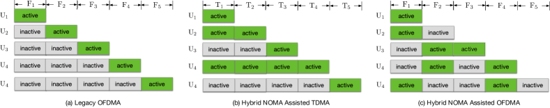
Figure 1: An illustration of the hybrid NOMA assisted OFDMA network. Compared to the TDMA case studied in [9, 11], the patten of resource allocation in the OFDMA case is more complex. For example, in TDMA, a user chooses to use either all the time slots (i.e., the hybrid NOMA mode) or just its own TDMA time slot (i.e., pure OMA), where ${\rm T}_{m}$ denotes the $m$-th time slot. But in OFDMA, a user, e.g., ${\rm U}_{2}$, may adopt the pure NOMA mode, and the time slots a user chooses to use are necessarily continuous.

The aim of this paper is to reduce the OFDMA users’ uplink power consumption by applying hybrid NOMA, as shown in Fig. 1. In particular, each user can still use the subcarrier that is allocated to it in the OFDMA legacy system, but a more energy constrained user is provided the access to more subcarriers. For example, ${\rm U}_{m}$ can still use its own OFDMA subcarrier, ${\rm F}_{m}$, but also has access to ${\rm F}_{i}$, $1\leq i\leq m$. As such, the most energy constrained user, ${\rm U}_{M}$, can have access to all subcarriers, whereas the least energy constrained user, ${\rm U}_{1}$, can use a single subcarrier only.

Therefore, at subcarrier ${\rm F}_{n}$, the base station receives the signals simultaneously transmitted by ${\rm U}_{i}$, $n\leq i\leq M$. The base station carries out successive interference cancellation (SIC) by employing the users’ diverse energy profiles, e.g., at subcarrier ${\rm F}_{n}$, ${\rm U}_{M}$’s signal is decoded first and ${\rm U}_{1}$’s signal is decoded last. With the used SIC decoding strategy, and assuming additive white Gaussian noise (AWGN), ${\rm U}_{m}$’s signal on ${\rm F}_{n}$ can be decoded with the following achievable data rate:

$$R_{m,n}=\log\left(1+\frac{h_{m,n}P_{m,n}}{\sum^{m-1}_{j=n}h_{j,n}P_{j,n}+1}\right),$$ (1)

where $P_{m,n}$ denotes ${\rm U}_{m}$’s transmit power on ${\rm F}_{n}$, and the noise power is assumed to be normalized. It is worthy pointing out that with the used SIC strategy, ${\rm U}_{m}$’s achievable data rate on ${\rm F}_{m}$ is simply $\log\left(1+{h_{m,m}P_{m,m}}\right)$, which is identical to the user’s data rate in OFDMA.

Because of the energy constrained nature of the considered uplink scenario, the following power minimization problem is considered in this paper:

$$\underset{P_{m,n}\geq 0}{\rm{min}} \quad\sum^{M}_{m=1}\sum^{m}_{n=1}P_{m,n}$$ (P1a)

$$s.t. \quad\sum^{m}_{n=1}R_{m,n}\geq R,\quad 1\leq m\leq M.$$ (P1b)

Remark 1: Similar to the hybrid NOMA schemes considered in [9, 11], problem (P1) leads to a general transmission framework, where the modes of pure OMA and pure NOMA can be obtained as special cases by adopting different choices of the power allocation coefficients, $P_{m,n}$.

Remark 2: The optimal solution of problem (P1) leads to a more complex resource allocation patten than its counterpart in the TDMA case, as illustrated in Fig. 1. For example, in H-NOMA-TDMA, the pure NOMA mode is always suboptimal, and a user always uses the bandwidth resource block (i.e, the time slot) that is assigned to it in OMA. However, in H-NOMA-OFDMA, the use of pure NOMA may outperform both hybrid NOMA and pure OMA. Another example is that for the uplink TDMA case with equal-duration time slots, i.e., the time slot durations are not optimized, the use of pure OMA is always optimal. In the OFDMA case, the pure OMA solution is rarely optimal, particularly if there is a large number of users, as will be shown in the next section.

Remark 3: The fact that a user’s channel gains on different subcarriers are different, i.e., for ${\rm U}_{m}$, $h_{m,1}\neq\cdots\neq h_{m,m}$, leads to the availability of the frequency diversity [24]. The proposed hybrid NOMA scheme can effectively utilize the frequency diversity inherent in the OFDMA legacy network, and ensures that a user that is more energy constrained consumes less energy for its uplink transmission, as shown in the next section. It is important to note that in TDMA, there is a dilemma associated with using such diversity as noted in the introduction. In particular, it is preferable to exploit such diversity as it can significantly reduce energy consumption. However, the use of such diversity requires the base station to know the users’ future CSI, which is challenging in practice.

III Performance Analysis: An Optimization Perspective

In this section, the properties of H-NOMA-OFDMA transmission are analyzed from an optimization perspective. In particular, tools from convex optimization are used to characterize the important features of the optimal solution of problem (P1), and address the issues of whether hybrid NOMA can outperform pure OMA and pure NOMA.

III-A Optimality of Pure OMA

It is straightforward to show that problem (P1) is not a convex optimization problem since the constraints in (P1a) are not convex. Therefore, it is challenging to obtain a closed-form expression for the optimal solution of problem (P1). However, it is important to point out that the Karush–Kuhn–Tucker (KKT) conditions can still be used as an optimality certificate for the solutions of this non-convex optimization problem [25]. By using this fact, insights into H-NOMA-OFDMA transmission can be obtained, as shown in the following lemma.

$\mathbf{Lemma}$ 1.

A necessary condition for the pure OMA solution, i.e., $P_{m,m}=\frac{e^{R}-1}{h_{m,m}}$ and $P_{m,n}=0$ for $m\neq n$, to be the optimal solution of problem (P1) is given by

$$h_{m,n}\leq h_{m,m},\quad 1\leq n\leq m-1,1\leq m\leq M.$$ (2)

Proof.

See Appendix A. ∎

The use of Lemma 1 immediately leads to the following corollary regarding the optimality of the pure OMA solution in practice.

$\mathbf{Corollary}$ 1.

Assuming that the users’ channel gains at different subcarriers are i.i.d., the probability that the pure OMA mode is optimal approaches zero if $M\rightarrow\infty$.

Proof.

Lemma 1 shows that a necessary condition for the pure OMA solution to be optimal is given by $h_{m,n}\leq h_{m,m}$, for $1\leq n\leq m-1$ and $1\leq m\leq M$. Because the users’ channel gains are assumed to be i.i.d., the probability of the event that this condition holds is given by

$$\mathbb{P}^{\rm OMA}= \mathbb{P}\left(h_{m,n}\leq h_{m,m},\quad 1\leq n\leq m-1,1\leq m\leq M\right)$$

$$= \prod^{M}_{m=2}\prod^{m-1}_{n=1}\mathbb{P}\left(h_{m,n}\leq h_{m,m}\right)$$

$$= \prod^{M}_{m=2}\frac{1}{2^{m-1}}=\frac{1}{2^{\frac{M(M-1)}{2}}}\rightarrow 0,$$ (3)

if $M\rightarrow\infty$. The proof of the corollary is complete. ∎

Remark 4: Corollary 1 illustrates an important difference between the applications of hybrid NOMA to TDMA and OFDMA networks. Recall that for the uplink TDMA case, if the time slot durations are not optimized, pure OMA outperforms both hybrid NOMA and pure NOMA [9, 11]. However, for the uplink OFDMA case, Corollary 1 demonstrates that the NOMA schemes outperform pure OMA, particularly for situations in which the number of users is very large.

III-B Optimality of Pure NOMA

As noted in the introduction, in studies of hybrid NOMA assisted TDMA, pure NOMA has been shown to be suboptimal [9, 11]. However, in the context of OFDMA, the use of the pure NOMA mode can be optimal, as shown in the following. Due to the complex and random patterns of the hybrid NOMA subcarrier allocation, a closed-form expression for the pure NOMA solution cannot be obtained. For example, consider a particular pure NOMA solution, where all the users use ${\rm F}_{1}$ only, i.e., $P_{m,1}\neq 0$, for $1\leq m\leq M$, and the users’ remaining power allocation coefficients are zero. For this particular pure NOMA case, problem P1 can be recast as follows:

$$\underset{P_{m,n}\geq 0}{\rm{min}} \quad\sum^{M}_{m=1}P_{m,1}$$ (P2a)

$$s.t. \quad\log\left(1+\frac{h_{m,1}P_{m,1}}{\sum^{m-1}_{j=1}h_{j,1}P_{j,1}+1}\right)\geq R,1\leq m\leq M,$$

which is equivalent to the following form:

$$\underset{P_{m,n}\geq 0}{\rm{min}} \quad\sum^{M}_{m=1}P_{m,1}$$ (P3a)

$$s.t. \quad h_{m,1}P_{m,1}\geq\phi\sum^{m-1}_{j=1}h_{j,1}P_{j,1}+\phi,1\leq m\leq M,$$

where $\phi=e^{R}-1$. Problem (P3) is a linear program that can be solved numerically, but it is challenging to obtain a closed form expression for its optimal solution. Therefore, in the following, we consider the case in which the first $M-1$ users choose the OMA mode, and the last user ${\rm U}_{M}$ chooses the pure NOMA mode, i.e., its dedicated OMA subcarrier is not used. Because the first $M-1$ users choose the OMA mode, problem (P1) can be simplified as follows:

$$\underset{1\leq n\leq M-1}{\text{arg }}\text{min} \quad P_{M,n}$$ (P4a)

$$s.t. \quad R_{M,n}\geq R.$$ (P4b)

Recall that $R_{M,n}=\log\left(1+\frac{h_{M,n}P_{M,n}}{\sum^{M-1}_{j=n}h_{j,n}P_{j,n}+1}\right)$. If the first $M-1$ users choose the OMA mode, $R_{M,n}$ can be simplified as follows:

$$R_{M,n}=\log\left(1+\frac{h_{M,n}P_{M,n}}{h_{n,n}P_{n,n}+1}\right)=\log\left(1+\frac{h_{M,n}P_{M,n}}{e^{R}}\right).$$ (4)

Because ${\rm U}_{M}$ suffers the same amount of interference during the first $M-1$ subcarriers, i.e., $h_{n,n}P_{n,n}+1=e^{R}$, for $1\leq n\leq M-1$, the optimal solution of problem (P4) is simply $n^{*}=\underset{1\leq n\leq M-1}{\text{arg max}h_{M,n}}$, i.e., the user chooses the best subcarrier. Without loss of generality, assume that $h_{M,1}\geq h_{M,i}$, $2\leq i\leq M$, which means $n^{*}=1$ and the corresponding pure NOMA solution is $P_{m,m}=\frac{e^{R}-1}{h_{m,m}}$, $1\leq m\leq M-1$, $P_{M,1}=\frac{e^{R}(e^{R}-1)}{h_{M,1}}$, and the other power coefficients are zero.

$\mathbf{Lemma}$ 2.

A necessary conditions for the considered pure NOMA solution to be optimal to problem (P1) are give by

$$\left\{\begin{array}[]{l}\frac{h_{m,n}}{h_{m,m}}\leq 1,\quad 1\leq n\leq m\leq M-1\\ \frac{h_{M,n}}{h_{M,1}}\leq 1,\quad 2\leq n\leq M-1\\ e^{R}h_{M,M}\leq h_{M,1}\end{array}\right..$$ (8)

Proof.

See Appendix B. ∎

We note that the considered pure NOMA solution is obtained with the condition that $h_{M,1}\geq h_{M,i}$, $2\leq i\leq M$, which is weaker than the one in Lemma 2, since $e^{R}h_{M,M}\leq h_{M,1}$ implies $h_{M,M}<e^{R}h_{M,M}\leq h_{M,1}$.

Remark 5: Lemma 2 shows that it is possible for a user to adopt the pure NOMA model in H-NOMA-OFDMA. Lemma 2 is also useful to illustrate another important difference between hybrid NOMA assisted OFDMA and TDMA. For the TDMA case, a user’s channel does not change over the $M$ time slots, and therefore, Lemma 2 is still applicable, but with the changes that $h_{m,1}=\cdots=h_{m,m}$. Therefore, the conditions in (12) can be simplified as follows:

$$\left\{\begin{array}[]{l}1\leq 1,\quad 1\leq n\leq m\leq M-1\\ 1\leq 1,\quad 2\leq n\leq M-1\\ e^{R}\leq 1\end{array}\right..$$ (12)

Because the last condition can never be met, a user will never choose the pure NOMA mode in the TDMA case, a conclusion consistent to those made in [9, 11].

III-C Successive Resource Allocation

Similar to [9, 11], a low-complexity algorithm can be developed to find a sup-optimal solution of problem (P1), by utilizing the successive nature of the SIC decoding strategy at the base station. In particular, the proposed successive resource allocation algorithm consists of $M$ stages, where during the $m$-th stage, the following optimization problem is solved:

$$\underset{P_{m,n}\geq 0}{\rm{min}} \quad\sum^{m}_{n=1}P_{m,n}$$ (P5a)

$$s.t. \quad\sum^{m}_{n=1}\log\left(1+\frac{h_{m,n}P_{m,n}}{\sum^{m-1}_{j=n}h_{j,n}P_{j,n}+1}\right)\geq R,$$ (P5b)

where the parameters, $P_{i,n}$, $i<m$, are obtained from the previous stages. Because $P_{i,n}$, $i<m$, are fixed, it is straightforward to show that problem (P5) is a convex optimization problem, and hence can be efficiently solved by those off-shelf optimization solvers.

Unlike the hybrid NOMA cases in [9, 11], a closed form expression for the successive resource allocation solution is challenging to obtain in the general case. However, insightful understandings can be obtained for the two-user special case. In particular, the optimality of the proposed successive resource allocation algorithm in the two-user special case is shown in the following lemma.

$\mathbf{Lemma}$ 3.

For the two-user special case, the solution obtained by the proposed successive resource allocation algorithm is optimal for problem (P1).

Proof.

This lemma can be proved by the method of contradiction. Denote the optimal solutions of problem (P1) by $P_{1,1}^{*}$, $P_{2,1}^{*}$ and $P_{2,2}^{*}$, and the solutions of successive resource allocation by $P_{1,1}^{\rm SRA}$, $P_{2,1}^{\rm SRA}$ and $P_{2,2}^{\rm SRA}$, respectively. Assume that $P_{1,1}^{*}+P_{2,1}^{*}+P_{2,2}^{*}<P_{1,1}^{\rm SRA}+P_{2,1}^{\rm SRA}+P_{2,2}^{\rm SRA}$.

First note that by using the proposed resource allocation algorithm, ${\rm U}_{1}$’s power allocation is simply its OMA choice, i.e., $P_{1,1}^{\rm SRA}=\frac{e^{R}-1}{h_{1,1}}$, which is the minimal transmit power for ${\rm U}_{1}$ to meet the target data rate $R$. Therefore, $P_{1,1}^{\rm SRA}\leq P_{1,1}^{*}$, which means that $P_{2,1}^{*}+P_{2,2}^{*}<P_{2,1}^{\rm SRA}+P_{2,2}^{\rm SRA}$ in order to ensure $P_{1,1}^{*}+P_{2,1}^{*}+P_{2,2}^{*}<P_{1,1}^{\rm SRA}+P_{2,1}^{\rm SRA}+P_{2,2}^{\rm SRA}$. However, $P_{2,1}^{\rm SRA}$ and $P_{2,2}^{\rm SRA}$ are optimal solutions of the following optimization problem:

$$\underset{P_{2,n}\geq 0}{\rm{min}} \quad P_{2,1}+P_{2,2}$$ (P6a)

$$s.t. \quad\log\left(1+\frac{h_{2,1}P_{2,1}}{h_{1,1}P_{1,1}^{\rm SRA}+1}\right)+\log\left(1+h_{2,2}P_{2,2}\right)\geq R.$$

Comparing problem (P6) to the following problem:

$$\underset{P_{2,n}\geq 0}{\rm{min}} \quad P_{2,1}+P_{2,2}$$ (P7a)

$$s.t. \quad\log\left(1+\frac{h_{2,1}P_{2,1}}{h_{1,1}P_{1,1}^{*}+1}\right)+\log\left(1+h_{2,2}P_{2,2}\right)\geq R,$$

one can notice that the feasibility region of problem (P7) is no larger than that of (P6) since $P_{1,1}^{\rm SRA}\leq P_{1,1}^{*}$. Therefore, $P_{2,1}^{*}+P_{2,2}^{*}<P_{2,1}^{\rm SRA}+P_{2,2}^{\rm SRA}$ cannot be true. The proof of the lemma is complete. ∎

By using Lemma 3, a closed-form expression for the optimal solution of problem (P1) can be obtained for the two-user special case, as shown in the following lemma.

$\mathbf{Lemma}$ 4.

For the two-user special case, an optimal solution of problem (P1) can be obtained as follows:

$$\left\{\begin{array}[]{ll}\text{Pure OMA mode:}&\text{if }\frac{h_{2,2}}{h_{2,1}}\geq 1\\ \text{Pure NOMA mode:}&\text{if }\frac{h_{2,2}}{h_{2,1}}\leq e^{-2R}\\ \text{Hybrid NOMA mode:}&\text{if }e^{-2R}\leq\frac{h_{2,2}}{h_{2,1}}<1\\ \end{array}\right.$$ (16)

where $P_{1,1}^{\rm*}=\frac{e^{R}-1}{h_{1,1}}$, for the hybrid NOMA mode, $P_{2,1}^{\rm*}=\frac{e^{R}}{\sqrt{h_{2,1}h_{2,2}}}-\frac{e^{R}}{h_{2,1}}$ and $P_{2,2}^{\rm*}=\frac{e^{R}}{\sqrt{h_{2,1}h_{2,2}}}-\frac{1}{h_{2,2}}$, for the pure NOMA mode, $P_{2,1}^{\rm*}=\frac{e^{R}(e^{R}-1)}{h_{2,1}}$ and $P_{2,2}^{\rm*}=0$, for the pure OMA mode, $P_{2,1}^{\rm*}=0$ and $P_{2,2}^{\rm*}=\frac{e^{R}-1}{h_{2,2}}$.

Proof.

See Appendix C. ∎

Remark 6: Lemma 4 demonstrates how challenging it can be to obtain closed-form expressions for optimal H-NOMA-OFDMA transmission, since even for the simple two-user special case, there are three possible expressions.

IV Performance Analysis: A Statistical Perspective

In the previous section, the features of H-NOMA-OFDMA have been revealed from the optimization perspective, where optimality conditions have been established for different transmission modes. These results are useful to understand under which conditions hybrid NOMA outperforms the other transmission modes, particularly pure OMA. This section focuses on the following question - how large can the performance gain of hybrid NOMA over pure OMA be? In particular, two new criteria, namely the power outage probability and the power diversity gain, are introduced to quantitize the performance gain of hybrid NOMA over OMA.

Formally, the power outage probability is defined as the probability that, in order to meet the target data rate, a user needs more transmit power than its power budget, denoted by $\rho$. Take OMA transmission as an example, where the power outage probability for ${\rm U}_{m}$ is given by

$$\mathbb{P}^{\rm out}_{m}= \mathbb{P}\left(P_{m}^{\rm OMA}\geq\rho\right)=\mathbb{P}\left(\frac{e^{R}-1}{h_{m,m}}\geq\rho\right)$$ (17)

$$= \mathbb{P}\left(\log\left(1+\rho h_{m,m}\right)\leq R\right),$$

which shows that for OMA, the power outage probability is equivalent to the standard outage probability [22]. Similar to the conventional outage diversity gain [23], ${\rm U}_{m}$’s power diversity gain can be defined as follows:

$$d=-\underset{\rho\rightarrow\infty}{\lim}\frac{\log\mathbb{P}_{m}^{\rm out}}{\log\rho}.$$ (18)

These two proposed metrics are useful for measuring how the users’ predefined energy profiles can be met in dynamic fading scenarios. For example, with a smaller power outage probability and a larger power diversity gain, a communication system is more robust to meet the users’ predefined energy profiles.

Two case studies will be carried out in this section by using these two performance evaluation metrics to illustrate the performance gain of hybrid NOMA over OMA.

IV-A The Two-User Special Case

We first consider the special case of two users, because a closed-form expression for the optimal solution of problem (P1) is available in this case. Note that with H-NOMA-OFDMA, ${\rm U}_{1}$’s transmit power is the same as its OMA transmit power. Therefore, only ${\rm U}_{2}$’s transmit power is considered in the following, where the corresponding power outage probability is given by

$$\mathbb{P}^{\rm out}_{2}=\mathbb{P}\left(P_{2,1}+P_{2,2}\geq\rho\right).$$ (19)

The following lemma provides a high signal-to-noise ratio (SNR) approximation of ${\rm U}_{2}$’s power outage probability.

$\mathbf{Lemma}$ 5.

At high SNR, i.e., $\rho\rightarrow\infty$, ${\rm U}_{2}$’s power outage probability can be approximated as follows:

$$\mathbb{P}^{\rm out}\approx \frac{(e^{R}-1)^{2}}{\rho^{2}}+\frac{\tau}{\rho^{2}},$$ (20)

where $\tau$ is a constant not related to $\rho$, $\tau=\int^{e^{R}}_{1}\frac{y-1}{\rho}\left(\min\left\{e^{2R},g_{2}(y)\right\}-\max\left\{1,g_{1}(y)\right\}\right)dy$, $g_{1}(y)=\frac{2e^{2R}-e^{R}y-2e^{R}\sqrt{e^{2R}-e^{R}y}}{y^{2}}$, and $g_{2}(y)=\frac{2e^{2R}-e^{R}y+2e^{R}\sqrt{e^{2R}-e^{R}y}}{y^{2}}$

Proof.

See Appendix D. ∎

By using Lemma 5, the following corollary for ${\rm U}_{2}$’s power diversity order can be straightforwardly obtained.

$\mathbf{Corollary}$ 2.

By using hybrid NOMA assisted OFDMA, ${\rm U}_{2}$’s power diversity order is $2$, where the power diversity order of pure OFDMA is $1$.

Remark 7: Lemma 5 and Corollary 2 demonstrate that the use of hybrid NOMA can significantly reduce the OFDMA uplink energy consumption, and more robustly meet the users’ stringent energy constraints. The reason for this performance gain can be explained by the following extreme example. Suppose that ${\rm U}_{2}$’s channel gain on ${\rm F}_{2}$ is in deep fading, i.e., $h_{2,2}\rightarrow 0$. The use of OMA leads to a singular energy situation, i.e., the user needs to use infinite transmit power. However, by using hybrid NOMA, this singularity issue can be avoided, since ${\rm U}_{2}$ can simply discard ${\rm F}_{2}$ and rely on ${\rm F}_{1}$ only. Following steps similar to those in the proof of Lemma 5 and using the fact that $h_{2,1}=h_{2,2}$ for the TDMA case, the following corollary can be obtained.

$\mathbf{Corollary}$ 3.

By using hybrid NOMA assisted TDMA, ${\rm U}_{2}$’s power diversity order is $1$.

Corollary 3 illustrates another difference between the applications of hybrid NOMA to TDMA and OFDMA systems, which is due to the use of the users’ dynamic channel conditions.

IV-B A Multi-User Special Case

Because a closed-form expression for the optimal solution of problem (P1) is not available for the general multi-user case, we focus on the pure NOMA solution considered in Section III-A, which offers important insights into general hybrid NOMA transmission. In particular, assume that the first $M-1$ users adopt the OMA mode, and ${\rm U}_{M}$ chooses ${\rm F}_{1}$ only, where it is assumed that $h_{M,1}\geq h_{m,i}$, $2\leq i\leq M$. Therefore, the corresponding power allocation solution is $P_{m,m}=\frac{e^{R}-1}{h_{m,m}}$, $1\leq m\leq M-1$, $P_{M,1}=\frac{e^{R}(e^{R}-1)}{h_{M,1}}$, and the other power coefficients are zero.

With this considered NOMA solution, ${\rm U}_{M}$’s power outage probability is given by

$$\mathbb{P}_{M}^{\rm out}= \mathbb{P}\left(\frac{e^{R}(e^{R}-1)}{h_{M,1}}\geq\rho,e^{R}h_{M,M}\leq h_{M,1},\right.$$ (21)

$$\left.h_{M,1}\geq h_{m,i},2\leq i\leq M\right),$$

where the condition in Lemma 2 is used. Again applying the complex Gaussian distribution assumption, the users’ unordered channel gains are i.i.d. exponentially distributed. Because $h_{M,1}\geq h_{m,i}$, $2\leq i\leq M-1$, the probability density function (pdf) of $h_{M,1}$ is given by $f(x)=(M-1)\left(1-e^{-x}\right)^{M-2}e^{-x}$. Therefore, ${\rm U}_{M}$’s power outage probability can be obtained as follows:

$$\mathbb{P}_{M}^{\rm out}= \mathbb{P}\left(e^{R}h_{M,M}\leq h_{M,1}\leq\frac{e^{R}(e^{R}-1)}{\rho},\right.$$ (22)

$$\left.h_{M,1}\geq h_{m,i},2\leq i\leq M\right)$$

$$= \int^{\frac{e^{R}-1}{\rho}}_{0}e^{-y}\int^{\frac{e^{R}(e^{R}-1)}{\rho}}_{e^{R}y}(M-1)\left(1-e^{-x}\right)^{M-2}e^{-x}dxdy.$$

With some straightforward algebraic manipulations, the outage probability can be obtained as follows:

$$\mathbb{P}_{M}^{\rm out}= -\left(1-e^{-\frac{e^{R}(e^{R}-1)}{\rho}}\right)^{M-1}\left(1-e^{-\frac{e^{R}-1}{\rho}}\right)$$ (23)

$$+\sum^{M-1}_{i=0}{M-1\choose i}(-1)^{i}\left(1-e^{-\left(1+ie^{R}\right)\frac{e^{R}-1}{\rho}}\right).$$

Following steps similar to those in the proof for Lemma 5, ${\rm U}_{M}$’s power outage probability can be approximated as follows:

$$\mathbb{P}_{M}^{\rm out}\approx \frac{e^{(M-1)R}(e^{R}-1)^{M}}{\rho^{M}}+\frac{e^{(M-1)R}}{M}\frac{(e^{R}-1)^{M}}{\rho^{M}},$$ (24)

which means that the power diversity order experienced by ${\rm U}_{M}$ is $M$. Recall that the power diversity order of OMA is only $1$, which means that the use of hybrid NOMA can significantly reduce ${\rm U}_{M}$’s energy consumption. Our simulation results show that by using hybrid NOMA, ${\rm U}_{i}$’s power diversity order is larger than ${\rm U}_{j}$’s power diversity order, for $i>j$, which not only justifies the adopted SIC decoding order, but also illustrates the capability of hybrid NOMA to meet the users’ different energy profiles.

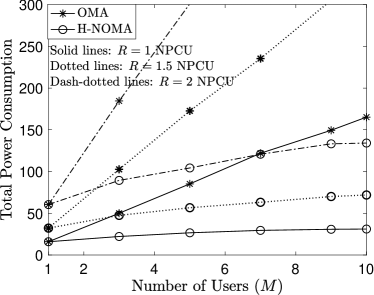
Figure 2: The total power consumption achieved by hybrid NOMA assisted OFDMA, where the users’ channel gains are assumed to be complex Gaussian distributed with zero mean and unit variance. NPCU denotes nats per channel use, and $\epsilon=10^{-5}$.

V Numerical Results

In this section, the performance of H-NOMA-OFDMA is demonstrated using computer simulation, where the accuracy of the developed analytical results is also examined. Two metrics, namely the averaged total power consumption and the power outage probability, are used for performance evaluation in the following two subsections, respectively. NPCU denotes nats per channel use.

V-A Averaged Total Power Consumption

In Fig. 2, the performance of H-NOMA-OFDMA is shown as a function of the number of the users, $M$. Recall that the users’ channels are assumed to be i.i.d. complex Gaussian random variables with zero means and unit variances, which means that the averaged power consumption for both OMA and NOMA will be infinite, as illustrated in the following. Take OMA as an example, where $\mathcal{E}_{h_{m,m}}\left\{P_{m}^{\rm OMA}\right\}=\int^{\infty}_{0}\frac{e^{R}-1}{x}e^{-x}dx\rightarrow\infty$. In order to avoid this singularity issue, it is assumed that $h_{m,n}\geq\epsilon$, where $\epsilon=10^{-5}$ is used in Fig. 2. As can be seen from the figure, for the case of $M>1$, the use of hybrid NOMA can significantly reduce the power consumption of OFDMA systems. The performance gain of NOMA over OMA can be further increased by increasing the target data rate. Furthermore, Fig. 2 shows that the total power consumption of OMA grows linearly with the number of the users, since $\mathcal{E}_{h_{m,m}}\left\{\sum^{M}_{m=1}P_{m}^{\rm OMA}\right\}=M\mathcal{E}_{h_{m,m}}\left\{P_{m}^{\rm OMA}\right\}$. However by using hybrid NOMA, there is only a slight increase in power consumption when the number of the users is increased. Therefore, the performance gain of NOMA over OMA becomes significantly larger if there are more users participating in the NOMA cooperation, which makes H-NOMA-OFDMA particularly appealing for umMTC.

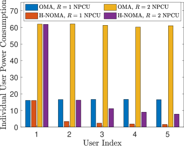
Figure 3: The users’ individual power consumption achieved by hybrid NOMA assisted OFDMA, where $\epsilon=10^{-4}$ and $M=5$.

In addition to its ability to reduce the total power consumption, H-NOMA-OFDMA can also meet the users’ diverse energy profiles, as shown in Fig. 3. Recall that in this study, ${\rm U}_{m}$ is assumed to be more energy constrained than ${\rm U}_{n}$, $n<m$. Fig. 3 demonstrates that the use of hybrid NOMA indeed ensures that ${\rm U}_{m}$ consumes less transmit power than ${\rm U}_{n}$, $n<m$, whereas with OMA, all the users use the same transmit power. This benefit is due to the fact that the use of hybrid NOMA ensures that a more energy constrained user has access to more bandwidth resources than a less energy constrained user. For example, ${\rm U}_{M}$ has access to all $M$ subcarriers, and hence has more degrees of freedom to reduce its energy consumption, compared to the other users. Fig. 3 also shows that the use of hybrid NOMA yields less power consumption than OMA, for all users except ${\rm U}_{1}$, which is consistent with the observation in Fig. 2.

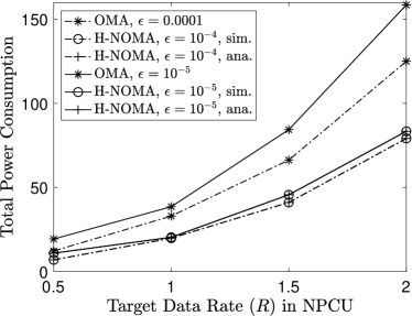
Figure 4: The performance of hybrid NOMA assisted OFDMA in the two-user special case, where the analytical results are based on Lemma 4.

Recall that for the two-user special case, the optimal solution of hybrid NOMA transmission can be obtained, as shown in Lemma 4. Therefore, Figs. 4 and 5 are provided to focus on this special case. As can be seen from the figures, the simulation results match the analytical results shown in Lemma 4, which verifies the accuracy of the developed analytical results and confirms the optimality of the closed-form solutions shown in Lemma 4. Recall that in Figs. 2 and 3, the users’ channel gains are clipped to avoid the energy singularity issue, i.e., $h_{m,n}\geq\epsilon$ is assumed. Fig. 4 is also provided to demonstrate the impact of this channel clipping on the performance of the considered transmission schemes. As can be seen from the figure, the use of smaller $\epsilon$ increases the performance gain of hybrid NOMA over OMA. Or in other words, this channel clipping assumption is more critical to OMA than hybrid NOMA. The reason for this observation is that in hybrid NOMA, a user has access to more subcarriers and hence is more robust to deep fading, where the use of deeply faded subcarriers can be avoided.

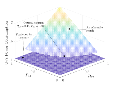
Figure 5: Comparison between the solutions obtained from Lemma 4 and an exhaustive search, where $\epsilon=10^{-5}$, $M=2$ and $R=1$ NPCU.

V-B Power Outage Probability

The two-user special case is considered first, because a closed-form expression for the power outage probability can be obtained in this special case. In Fig. 6, only ${\rm U}_{2}$’s power outage performance is shown, since ${\rm U}_{1}$ experiences the same performance in OMA and NOMA. As can be seen from the figure, the use of hybrid NOMA can significantly improve the power outage performance, compared to OMA, particularly at high SNR. In addition, Fig. 6 demonstrates that the analytical results match the simulation results at high SNR, which verifies the accuracy of Lemma 5. Furthermore, the slope of the user’s power outage probability in NOMA is larger than OMA, which confirms Corollary 2, i.e., the power diversity order of hybrid NOMA is larger than that of OMA.

The behavior of hybrid NOMA shown in Fig. 6 is closely related to that seen in Fig. 5, and together they reveal the key benefit to use hybrid NOMA. Recall that Fig. 5 shows that the use of a smaller $\epsilon$ increases the performance gain of hybrid NOMA over OMA. Fig. 6 shows that the use of hybrid NOMA achieves a larger power diversity gain than OMA. These performance gains are due to the key feature of hybrid NOMA that a user is offered more transmission opportunities, e.g., subcarriers, compared to OMA. Again take the two-user scenario as an example. With OMA, ${\rm U}_{2}$ has to rely on a single subcarrier for its transmission, which means that its transmit power has to be very large if it suffers deep fading at the assigned subcarrier. With hybrid NOMA, the user has access to two subcarriers. If the user suffers deep fading at one subcarrier, it can discard this subcarrier and use the other one, which is the reason for the substantial performance gain of hybrid NOMA at small $\epsilon$ shown in Fig. 5 and the large power diversity gain shown in Fig. 6.

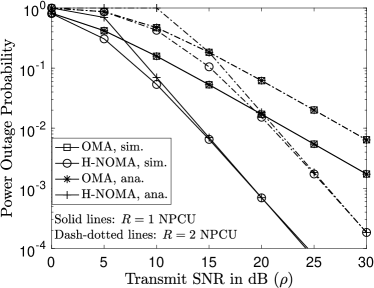
Figure 6: ${\rm U}_{2}$’s power outage probability achieved by hybrid NOMA assisted OFDMA, where the two-user special case is considered. The analytical results are based on Lemma 5.

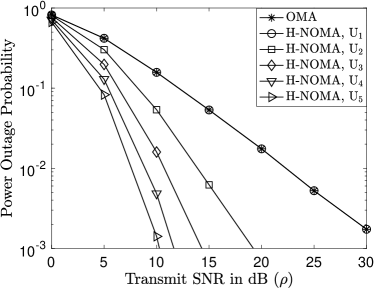
(a) $R=1$ NPCU

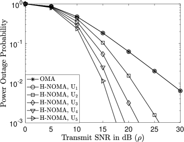
(b) $R=2$ NPCU

Figure 7: The users’ individual power outage performance in a general multi-user scenario, where $M=5$.

In Fig. 7, a general multi-user scenario is considered, where the users’ individual power outage probabilities are shown as functions of the transmit SNR. Because the users’ channel gains are i.i.d., the users’ OMA power outage probabilities are the same, which is the reason why there is a single curve for the OMA case. As can be seen from the figure, with hybrid NOMA, the users’ power outage probabilities are appropriate for their energy profiles. In particular, recall that ${\rm U}_{m}$ is assumed to be more energy constrained than ${\rm U}_{n}$, $n<m$. Fig. 7(a) shows that for the case with $R=1$ NPCU, to realize a power outage probability of $10^{-2}$, ${\rm U}_{1}$, the user that is the least energy constrained, requires a transmit SNR of $23$ dB, whereas ${\rm U}_{5}$, the user that is the most energy constrained, requires a transmit SNR of $7$ dB only, i.e., for this considered case, ${\rm U}_{5}$’s transmit power is just one-fifth of ${\rm U}_{1}$’s transmit power. Similar performance gains can also be observed from Fig. 7(b) for the case with $R=2$ NPUC. It is worthy pointing out that by applying the proposed hybrid NOMA scheme, ${\rm U}_{1}$’s achievable data rate is the same as that of OMA, which is the reason why in Fig. 7, ${\rm U}_{1}$’s power outage probabilities in OMA and NOMA are the same.

VI Conclusions

In this paper, hybrid NOMA assisted OFDMA uplink transmission has been investigated. In particular, the impact of the unique feature of H-NOMA-OFDMA, i.e., the availability of dynamic user channel conditions, on the system performance has been analyzed from two perspectives. From the optimization perspective, analytical results have been developed to show that with H-NOMA-OFDMA, the pure OMA mode is rarely adopted by the users, and the pure NOMA mode could be optimal for minimizing the users’ energy consumption, which are different from those conclusions made in earlier studies of hybrid NOMA based on TDMA. From the statistical perspective, two new metrics, namely the power outage probability and the power diversity gain, have been developed to measure the performance gain of hybrid NOMA over OMA. The developed analytical results also demonstrate the capability of hybrid NOMA to meet users’ diverse energy profiles.

Appendix A Proof for Lemma 1

Recall that the KKT conditions are necessary for any optimal solutions, regardless of whether the optimization problem is convex. Therefore, the lemma can be proved by first finding the KKT conditions of problem (P1) and then obtaining the conditions for the pure OMA solution to satisfy the KKT conditions.

Note that the Lagrangian of problem (P1) can be obtained as follows:

$$L= \sum^{M}_{m=1}\sum^{m}_{n=1}P_{m,n}+\sum^{M}_{m=1}\lambda_{m}\left(R-\sum^{m}_{n=1}R_{m,n}\right)$$ (25)

$$-\sum^{M}_{m=1}\sum^{m}_{n=1}\lambda_{m,n}P_{m,n},$$

where $\lambda_{m}$ is the Lagrange multiplier for the constraint $\sum^{m}_{n=1}R_{m,n}\geq R$, $1\leq m\leq M$, and $\lambda_{m,n}$ is the Lagrange multiplier for the constraint $P_{m,n}\geq 0$. For problem (P1), the corresponding KKT conditions can be expressed as follows:

$$\left\{\begin{array}[]{l}\frac{\partial L}{\partial P_{m,n}}=0,\quad n\leq m\leq M,1\leq m\leq M\\ \lambda_{m}\left(R-\sum^{m}_{n=1}R_{m,n}\right)=0,\quad 1\leq m\leq M\\ \lambda_{m,n}P_{m,n}=0,\quad n\leq m\leq M,1\leq m\leq M\end{array}\right.,$$ (29)

where the primal feasibility conditions are omitted due to space limitations.

The challenging step to evaluate the KKT conditions of problem (P1) is to find the stationarity condition, i.e., $\frac{\partial L}{\partial P_{m,n}}=0$, due to the complicated expressions for $R_{m,n}$. In particular, the stationarity conditions can be expressed as follows:

$$\frac{\partial L}{\partial P_{m,n}}=1-\sum^{M}_{i=1}\lambda_{i}\frac{\partial}{\partial P_{m,n}}\sum^{i}_{j=1}R_{i,j}-\lambda_{m,n}.$$ (30)

A key observation that can be used to simplify the stationarity conditions is that $P_{m,n}$ has an impact on $R_{i,n}$, $m\leq i\leq M$, only. Therefore, $\frac{\partial R_{i,j}}{\partial P_{m,n}}=0$, if $j\neq n$, and $\frac{\partial R_{i,n}}{\partial P_{m,n}}=0$, if $1\leq i<m$. By using this observation, the stationarity condition can be simplified as follows:

$$\frac{\partial L}{\partial P_{m,n}}=1-\sum^{M}_{i=m}\lambda_{m}\frac{\partial R_{i,n}}{\partial P_{m,n}}-\lambda_{m,n}$$ (31)

$$=1-\lambda_{m,n}-\sum^{M}_{i=m}\lambda_{m}\frac{\partial}{\partial P_{m,n}}\log\left(1+\frac{h_{i,n}P_{i,n}}{\sum^{i-1}_{j=n}h_{j,n}P_{j,n}+1}\right),$$

for $n\leq m-1$. The special case of $n=m$ will be discussed later.

It is important to note that $P_{m,n}$ appears not only in the numerator of the signal-to-interference-plus-noise ratio (SINR) of $R_{m,n}$, but also in the denominator of the SINR of $R_{m,i}$, $m+1\leq i\leq M$. To facilitate the derivative calculation, the stationarity conditions needs to be further rewritten as follows:

$$\frac{\partial L}{\partial P_{m,n}}=1-\lambda_{m}\frac{\partial}{\partial P_{m,n}}\log\left(1+\frac{h_{m,n}P_{m,n}}{\sum^{m-1}_{j=n}h_{j,n}P_{j,n}+1}\right)$$

$$-\sum^{M}_{i=m+1}\lambda_{m}\frac{\partial}{\partial P_{m,n}}\log\left(1+\frac{h_{i,n}P_{i,n}}{\sum^{i-1}_{j=n}h_{j,n}P_{j,n}+1}\right)-\lambda_{m,n}.$$ (32)

With some straightforward algebraic manipulations, the stationarity conditions can be expressed as follows:

$$\frac{\partial L}{\partial P_{m,n}}= 1-\lambda_{m,n}-\lambda_{m}\frac{h_{m,n}}{1+\sum^{m}_{j=n}h_{j,n}P_{j,n}}$$ (33)

$$-\sum^{M}_{i=m+1}\lambda_{m}\frac{h_{m,n}}{1+\sum^{i}_{j=n}h_{j,n}P_{j,n}}$$

$$+\sum^{M}_{i=m+1}\lambda_{m}\frac{h_{m,n}}{1+\sum^{i-1}_{j=n}h_{j,n}P_{j,n}},$$

for $n\leq m-1$. For the special case $n=m$, the stationarity conditions in (32) needs to be rewritten as follows:

$$\frac{\partial L}{\partial P_{m,m}}=1-\lambda_{m,m}-\lambda_{m}\frac{\partial}{\partial P_{m,m}}\log\left(1+h_{m,m}P_{m,m}\right)$$

$$-\sum^{M}_{i=m+1}\lambda_{m}\frac{\partial}{\partial P_{m,m}}\log\left(1+\frac{h_{i,m}P_{i,m}}{\sum^{i-1}_{j=m}h_{j,m}P_{j,m}+1}\right).$$ (34)

It can be verified that the result in (33) is still applicable to this special case since $\frac{\partial}{\partial P_{m,m}}\log\left(1+h_{m,m}P_{m,m}\right)=\frac{h_{m,m}}{1+h_{m,m}P_{m,m}}$

Recall that the OMA solution is given by $P_{m,m}=\frac{e^{R}-1}{h_{m,m}}$, and $P_{m,n}=0$ for $n<m$ and $1\leq m\leq M$. By substituting the OMA solution into (33), the stationarity conditions can be simplified as follows:

$$\frac{\partial L}{\partial P_{m,n}}= 1-\lambda_{m,n}-\lambda_{m}\frac{h_{m,n}}{1+h_{n,n}P_{n,n}}$$ (35)

$$-\sum^{M}_{i=m+1}\lambda_{m}\frac{h_{m,n}}{1+h_{n,n}P_{n,n}}$$

$$+\sum^{M}_{i=m+1}\lambda_{m}\frac{h_{m,n}}{1+h_{n,n}P_{n,n}}$$

$$= 1-\lambda_{m,n}-\lambda_{m}\frac{h_{m,n}}{1+h_{n,n}P_{n,n}},$$

where the first step follows from the fact that $\sum^{i}_{j=n}h_{j,n}P_{j,n}=h_{n,n}P_{n,n}$ and $\sum^{i-1}_{j=n}h_{j,n}P_{j,n}=h_{n,n}P_{n,n}$ because $n\leq m\leq i-1$.

Therefore, with the pure OMA solution, the KKT conditions can be reduced to the following:

$$\left\{\begin{array}[]{l}1-\lambda_{m,n}-\lambda_{m}\frac{h_{m,n}}{1+h_{n,n}P_{n,n}}=0,n\leq m,1\leq m\leq M\\ \lambda_{m}\left(R-\sum^{m}_{n=1}R_{m,n}\right)=0,1\leq m\leq M\\ \lambda_{m,n}P_{m,n}=0,n\leq m\leq M,1\leq m\leq M\end{array}\right..$$ (39)

Note that the pure OMA solution satisfies the primary feasibility conditions, and ensures $R-\sum^{m}_{n=1}R_{m,n}=0$, $1\leq m\leq M$. Therefore, the use of the pure OMA solution simplifies the KKT conditions to the following form:

$$\left\{\begin{array}[]{l}1-\lambda_{m,n}-\lambda_{m}\frac{h_{m,n}}{1+h_{n,n}P_{n,n}}=0,n\leq m,1\leq m\leq M\\ \lambda_{m,n}P_{m,n}=0,n\leq m\leq M,1\leq m\leq M\end{array}\right..$$ (42)

By using the fact that $P_{m,m}=\frac{e^{R}-1}{h_{m,m}}$ means that $h_{m,m}P_{m,m}+1=e^{R}$, the KKT conditions can be further simplified as follows:

$$\left\{\begin{array}[]{l}1-\lambda_{m,n}-e^{-R}\lambda_{m}h_{m,n}=0,n\leq m,1\leq m\leq M\\ \lambda_{m,n}P_{m,n}=0,n\leq m\leq M,1\leq m\leq M\end{array}\right..$$ (45)

Recall that for the OMA case, $P_{m,m}=\frac{e^{R}-1}{h_{m,m}}$, and $P_{m,n}=0$ for $n<m$ and $1\leq m\leq M$, which means $\lambda_{m,m}=0$ for $1\leq m\leq M$. Therefore, the first part of the KKT conditions in (45) can be expressed as follows:

$$1-e^{-R}\lambda_{m}h_{m,m}=0,\quad 1\leq m\leq M,$$ (46)

which means that the Lagrange multipliers corresponding to the constraint $\sum^{m}_{n=1}R_{m,n}\geq R$, $\lambda_{m}$, can be obtained as follows:

$$\lambda_{m}=\frac{e^{R}}{h_{m,m}},\quad 1\leq m\leq M,$$ (47)

which are always positive. The Lagrange multipliers corresponding to zero power allocation coefficients can be obtained as follows:

$$\lambda_{m,n}=1-e^{-R}\lambda_{m}h_{m,n}=1-\frac{h_{m,n}}{h_{m,m}},$$ (48)

where $1\leq n\leq m-1$ and $1\leq m\leq M$. Therefore, a necessary condition for the pure OMA solution to be optimal is given by

$$1-\frac{h_{m,n}}{h_{m,m}}\geq 0\rightarrow\frac{h_{m,n}}{h_{m,m}}\leq 1,\quad 1\leq n\leq m-1.$$ (49)

The proof of the lemma is complete. ∎

Appendix B Proof for Lemma 2

By following the steps in the proof of Lemma 1, for the considered pure NOMA solution, the stationarity conditions can be simplified as follows:

$$\frac{\partial L}{\partial P_{m,n}}= 1-\lambda_{m,n}-\lambda_{m}\frac{h_{m,n}}{1+h_{n,n}P_{n,n}}.$$ (50)

Recall that the KKT conditions for problem (P1) are given by

$$\left\{\begin{array}[]{l}\frac{\partial L}{\partial P_{m,n}}=0,\quad n\leq m\leq M,1\leq m\leq M\\ \lambda_{m}\left(R-\sum^{m}_{n=1}R_{m,n}\right)=0,\quad 1\leq m\leq M\\ \lambda_{m,n}P_{m,n}=0,\quad n\leq m\leq M,1\leq m\leq M\end{array}\right..$$ (54)

By substituting the pure NOMA solution into (54), the KKT conditions can be simplified as follows:

$$\left\{\begin{array}[]{l}1-\lambda_{m,n}-e^{-R}\lambda_{m}h_{m,n}=0,\quad n\leq m\leq M,n\neq m\neq M\\ 1-\lambda_{M,M}-\lambda_{M}h_{M,M}=0\\ \lambda_{m,n}P_{m,n}=0,\quad n\leq m\leq M,1\leq m\leq M\end{array}\right..$$ (58)

Recall that the considered pure NOMA solution is $P_{m,m}=\frac{e^{R}-1}{h_{m,m}}$, $1\leq m\leq M-1$, $P_{M,1}=\frac{e^{R}(e^{R}-1)}{h_{M,1}}$, and the other power coefficients are zero. Therefore, for $\lambda_{m,m}=0$, $1\leq m\leq M-1$, the Lagrange multipliers corresponding to $\sum^{m}_{n=1}R_{m,n}\geq R$, $1\leq m\leq M-1$, are given by

$$1-e^{-R}\lambda_{m}h_{m,m}=0\rightarrow\lambda_{m}=\frac{e^{R}}{h_{m,m}},$$ (59)

which are always positive. The Lagrange multipliers corresponding to $\sum^{M}_{n=1}R_{M,n}\geq R$, $\lambda_{M}$, and the one corresponding to $P_{M,M}$, $\lambda_{M,M}$, are coupled as follows:

$$\left\{\begin{array}[]{l}1-\lambda_{M,M}-\lambda_{M}h_{M,M}=0\\ 1-e^{-R}\lambda_{M}h_{M,1}=0\end{array}\right.,$$ (62)

where the second equation follows from the fact that $\lambda_{M,1}=0$ since $P_{M,1}\neq 0$. By solving the above two equations, the two multipliers can be obtained as follows:

$$\lambda_{M,M}=1-\frac{e^{R}}{h_{M,1}}h_{M,M},\quad\lambda_{M}=\frac{e^{R}}{h_{M,1}}$$ (63)

Following steps similar to those in the proof of Lemma 1, the other multipliers can be obtained as follows:

$$\left\{\begin{array}[]{l}\lambda_{m,n}=1-\frac{h_{m,n}}{h_{m,m}},\quad 1\leq n\leq m\leq M-1\\ \lambda_{M,n}=1-\frac{h_{M,n}}{h_{M,1}},\quad 2\leq n\leq M-1\end{array}\right..$$ (66)

Combining (63) and (66), the conditions shown in the lemma can be obtained, which concludes the proof. ∎

Appendix C Proof for Lemma 4

Recall that for the two-user special case, problem P5 can be simplified as follows:

$$\underset{P_{2,n}\geq 0}{\rm{min}} \quad P_{2,1}+P_{2,2}$$ (P8a)

$$s.t. \quad\log\left(1+\frac{h_{2,1}P_{2,1}}{h_{1,1}P_{1,1}+1}\right)+\log\left(1+h_{2,2}P_{2,2}\right)\geq R.$$

By using the fact that $P_{1,1}^{\rm SRA}=\frac{e^{R}-1}{h_{1,1}}$, problem (P8) can be simplified as follows:

$$\underset{P_{2,n}\geq 0}{\rm{min}} \quad P_{2,1}+P_{2,2}$$ (P9a)

$$s.t. \quad\log\left(1+e^{-R}h_{2,1}P_{2,1}\right)+\log\left(1+h_{2,2}P_{2,2}\right)\geq R.$$ (P9b)

First note that the Lagrangian of problem (P9) is given by

$$L= P_{2,1}+P_{2,2}-\sum^{3}_{i=2}\lambda_{i}P_{2,i-1}$$ (67)

$$+\lambda_{1}\left(R-\log\left(1+e^{-R}h_{2,1}P_{2,1}\right)-\log\left(1+h_{2,2}P_{2,2}\right)\right),$$

where $\lambda_{i}$, $1\leq i\leq 3$, denote the Lagrange multipliers, and the corresponding KKT conditions are given by

$$\left\{\begin{array}[]{l}1-\frac{\lambda_{1}e^{-R}h_{2,1}}{1+e^{-R}h_{2,1}P_{2,1}}-\lambda_{2}=0,\\ 1-\frac{\lambda_{1}h_{2,2}}{1+h_{2,2}P_{2,2}}-\lambda_{3}=0\\ R-\log\left(1+e^{-R}h_{2,1}P_{2,1}\right)-\log\left(1+h_{2,2}P_{2,2}\right)=0\end{array}\right..$$ (71)

It is challenging to directly establish necessary and sufficient condition for the hybrid NOMA solution to be optimal. Therefore, conditions for adopting the pure NOMA and OMA solutions are obtained first, as shown in the following.

C-1 Pure NOMA Solution

If the pure NOMA solution is used, ${\rm U}_{2}$ does not use ${\rm F}_{2}$, which means that problem (P9) can be simplified as follows:

$$\underset{P_{m,n}\geq 0}{\rm{min}} \quad P_{2,1}$$ (P10a)

$$s.t. \quad\log\left(1+e^{-R}h_{2,1}P_{2,1}\right)\geq R.$$ (P10b)

With some straightforward algebraic manipulations, the pure NOMA solution is obtained as follows:

$$P_{2,1}=\frac{e^{R}(e^{R}-1)}{h_{2,1}},\quad P_{2,2}=0.$$ (72)

An important part of Lemma 4 is to establish optimality conditions for different modes, and an optimality condition for the pure NOMA mode is established as follows. Because $P_{2,1}\neq 0$ and $P_{2,2}=0$, $\lambda_{2}=0$ and possibly $\lambda_{3}\neq 0$. By using the closed-form expressions of the pure NOMA solution, the KKT conditions can be rewritten as follows:

$$\left\{\begin{array}[]{l}1-\frac{\lambda_{1}e^{-R}h_{2,1}}{1+e^{-R}h_{2,1}\frac{e^{R}(e^{R}-1)}{h_{2,1}}}=0\\ 1-\lambda_{1}h_{2,2}-\lambda_{3}=0\end{array}\right.,$$ (75)

which yield the following closed-form expressions for the Lagrange multipliers:

$$\left\{\begin{array}[]{l}1-\lambda_{1}e^{-2R}h_{2,1}=0\rightarrow\lambda_{1}=\frac{e^{2R}}{h_{2,1}}\\ 1-\lambda_{1}h_{2,2}-\lambda_{3}=0\rightarrow\lambda_{3}=1-\frac{e^{2R}h_{2,2}}{h_{2,1}}\end{array}\right..$$ (78)

Because the considered optimization problem for the two-user special case is convex, the necessary and sufficient condition for pure NOMA to be optimal is given by

$$1-\frac{e^{2R}h_{2,2}}{h_{2,1}}\geq 0\rightarrow\frac{h_{2,2}}{h_{2,1}}\leq e^{-2R}.$$ (79)

C-2 Pure OMA Solution

Note that the pure OMA solution is simply given by

$$P_{2,1}=0,\quad P_{2,2}=\frac{e^{R}-1}{h_{2,2}}.$$ (80)

In order to establish the necessary and sufficient condition for the pure OMA solution to be optimal, closed-form expressions for the Lagrange multipliers are needed. Because $P_{2,2}\neq 0$, $\lambda_{3}=0$. By using the fact $\lambda_{3}=0$ and the closed-form expression for the pure OMA solution, the KKT conditions can be simplified as follows:

$$\left\{\begin{array}[]{l}1-\lambda_{1}e^{-R}h_{2,1}-\lambda_{2}=0\\ 1-\frac{\lambda_{1}h_{2,2}}{1+h_{2,2}\frac{e^{R}-1}{h_{2,2}}}=0\end{array}\right.,$$ (83)

which leads to the following closed-form expressions for the multipliers:

$$\left\{\begin{array}[]{l}1-\lambda_{1}e^{-R}h_{2,1}-\lambda_{2}=0\rightarrow\lambda_{2}=1-\frac{h_{2,1}}{h_{2,2}}\\ 1-e^{-R}\lambda_{1}h_{2,2}=0\rightarrow\lambda_{1}=\frac{e^{R}}{h_{2,2}}\end{array}\right..$$ (86)

Therefore, the necessary and sufficient condition for the optimality of pure OMA is given by

$$1-\frac{h_{2,1}}{h_{2,2}}\geq 0\rightarrow\frac{h_{2,1}}{h_{2,2}}\leq 1\rightarrow\frac{h_{2,2}}{h_{2,1}}\geq 1.$$ (87)

C-3 Hybrid NOMA Solution

Because tthe necessary and sufficient conditions for the optimality of the pure NOMA and OMA solutions have been established, the necessary and sufficient condition for hybrid NOMA to be optimal can be straightforwardly obtained as shown in the lemma. The remainder of the proof is to focus on how to obtain the closed-form expression for the hybrid NOMA solution. By ignoring the constraints, $P_{2,n}\geq 0$, the Lagrange of problem (P9) can be simplified as follows:

$$L= P_{2,1}+P_{2,2}$$ (88)

$$+\lambda\left(R-\log\left(1+e^{-R}h_{2,1}P_{2,1}\right)-\log\left(1+h_{2,2}P_{2,2}\right)\ \right),$$

where $\lambda$ is the only multiplier corresponding to the constraint (P9b). Therefore, the corresponding KKT conditions can be expressed as follows:

$$\left\{\begin{array}[]{l}1-\frac{\lambda e^{-R}h_{2,1}}{1+e^{-R}h_{2,1}P_{2,1}}=0\\ 1-\frac{\lambda h_{2,2}}{1+h_{2,2}P_{2,2}}=0\\ R-\log\left(1+e^{-R}h_{2,1}P_{2,1}\right)-\log\left(1+h_{2,2}P_{2,2}\right)=0\end{array}\right..$$ (92)

By combining the above KKT conditions, the following equality can be established:

$$R-\log\left(\lambda e^{-R}h_{2,1}\right)-\log\left(\lambda h_{2,2}\right)=0,$$ (93)

which means that the multiplier can be obtained as follows:

$$\lambda=\frac{e^{R}}{\sqrt{h_{2,1}h_{2,2}}}.$$ (94)

By substituting the expression for $\lambda$ into the first two equations in (92), the following is obtained:

$$1+e^{-R}h_{2,1}P_{2,1}= \lambda e^{-R}h_{2,1},$$ (95)

$$1+h_{2,2}P_{2,2}= \lambda h_{2,2},$$ (96)

which leads to a closed-form expression for the hybrid NOMA solution:

$$P_{2,1}=\frac{e^{R}}{\sqrt{h_{2,1}h_{2,2}}}-\frac{e^{R}}{h_{2,1}},$$ (97)

$$P_{2,2}=\frac{e^{R}}{\sqrt{h_{2,1}h_{2,2}}}-\frac{1}{h_{2,2}}.$$ (98)

The proof of the lemma is complete. ∎

Appendix D Proof for Lemma 5

Recall that all three transmission modes, namely pure OMA, pure NOMA and hybrid NOMA, could be adopted, which means that the power outage probability can be expressed as follows:

$$\mathbb{P}^{\rm out}_{2}= \mathbb{P}\left(E^{\rm OMA},\frac{h_{2,2}}{h_{2,1}}\geq 1\right)$$ (99)

$$+\mathbb{P}\left(E^{\rm NOMA},\frac{h_{2,2}}{h_{2,1}}\leq e^{-2R}\right)$$

$$+\mathbb{P}\left(E^{\rm Hybrid},e^{-2R}\leq\frac{h_{2,2}}{h_{2,1}}<1\right),$$

where $E^{\rm OMA}$, $E^{\rm NOMA}$, and $E^{\rm Hybrid}$ denote the power outage events associated to the three transmission modes, namely OMA, NOMA, and hybrid NOMA, respectively. The three outage cases will be analyzed separately in the following subsections.

D-1 Hybrid NOMA

For notational simplicity, define $\mathbb{P}_{1}\triangleq\mathbb{P}\left(E^{\rm OMA},\frac{h_{2,2}}{h_{2,1}}\geq 1\right)$, which can be evaluated as follows:

$$\mathbb{P}_{1}= \mathbb{P}\left(P_{2,1}+P_{2,2}\geq\rho,\frac{h_{2,2}}{h_{2,1}}\geq 1\right)$$ (100)

$$= \mathbb{P}\left(\frac{2e^{R}}{\sqrt{h_{2,1}h_{2,2}}}-\frac{e^{R}}{h_{2,1}}-\frac{1}{h_{2,2}}\geq\rho,e^{-2R}\leq\frac{h_{2,2}}{h_{2,1}}<1\right).$$

By defining $x_{1}=\sqrt{h_{2,1}}$ and $x_{2}=\sqrt{h_{2,2}}$, and with some algebraic manipulations, the outage probability can be expressed as follows:

$$\mathbb{P}_{1}= \mathbb{P}\left((\rho x_{2}^{2}+1)x_{1}^{2}-2e^{R}x_{2}x_{1}+e^{R}x_{2}^{2}\leq 0,\right.$$ (101)

$$\left.x_{1}e^{-R}\leq x_{2}<x_{1}\right).$$

Note that the roots of $(\rho x_{2}^{2}+1)x_{1}^{2}-2e^{R}x_{2}x_{1}+e^{R}x_{2}^{2}=0$ are given by

$$\frac{e^{R}x_{2}\pm x_{2}\sqrt{e^{2R}-e^{R}(\rho x_{2}^{2}+1)}}{\rho x_{2}^{2}+1}\geq 0,$$ (102)

where the following additional constraint is required:

$$e^{2R}-e^{R}(\rho x_{2}^{2}+1)\geq 0.$$ (103)

We note that the condition for the optimality of hybrid NOMA can be expressed as follows:

$$x_{1}e^{-R}\leq x_{2}<x_{1}\rightarrow x_{2}\leq x_{1}\leq e^{R}x_{2}.$$ (104)

Therefore, the considered outage probability $\mathbb{P}_{1}$ can be expressed as follows:

$$\mathbb{P}_{1}= \mathbb{P}\left(\frac{e^{R}x_{2}-x_{2}\sqrt{e^{2R}-e^{R}(\rho x_{2}^{2}+1)}}{\rho x_{2}^{2}+1}\right.$$ (105)

$$\left.\leq x_{1}\leq\frac{e^{R}x_{2}+x_{2}\sqrt{e^{2R}-e^{R}(\rho x_{2}^{2}+1)}}{\rho x_{2}^{2}+1},\right.$$

$$\left.e^{2R}-e^{R}(\rho x_{2}^{2}+1)\geq 0,x_{2}\leq x_{1}\leq e^{R}x_{2}\right).$$

By defining $f_{1}(x_{2})=\frac{e^{R}x_{2}-x_{2}\sqrt{e^{2R}-e^{R}(\rho x_{2}^{2}+1)}}{\rho x_{2}^{2}+1}$ and $f_{2}(x_{2})=\frac{e^{R}x_{2}+x_{2}\sqrt{e^{2R}-e^{R}(\rho x_{2}^{2}+1)}}{\rho x_{2}^{2}+1}$, the outage probability can be simplified as follows:

$$\mathbb{P}_{1}= \mathbb{P}\left(f_{1}(x_{2})\leq x_{1}\leq f_{2}(x_{2}),e^{2R}-e^{R}(\rho x_{2}^{2}+1)\geq 0,\right.$$

$$\left.x_{2}\leq x_{1}\leq e^{R}x_{2}\right)$$

$$= \mathbb{P}\left(f_{1}^{2}(x_{2})\leq x_{1}^{2}\leq f_{2}^{2}(x_{2})\right.$$

$$\left.x_{2}^{2}\leq\frac{e^{R}-1}{\rho},x_{2}^{2}\leq x_{1}^{2}\leq e^{2R}x_{2}^{2}\right).$$

By using the assumption that all the users’ channel gains are complex Gaussian distributed with zero mean and unit variance, the outage probability can be evaluated as follows:

$$\mathbb{P}_{1}= \int^{\frac{e^{R}-1}{\rho}}_{0}\left(e^{-\max\{z,f_{1}^{2}(\sqrt{z})\}}-e^{-\min\left\{e^{2R}z,f_{2}^{2}(\sqrt{z})\right\}}\right)e^{-z}dz.$$ (106)

By defining $y=\rho z+1$, the above integral can be simplified as follows:

$$\mathbb{P}_{1}= \int^{e^{R}}_{1}\left(e^{-\max\left\{\frac{y-1}{\rho},f_{1}^{2}\left(\sqrt{\frac{y-1}{\rho}}\right)\right\}}\right.$$ (107)

$$\left.-e^{-\min\left\{e^{2R}\frac{y-1}{\rho},f_{2}^{2}\left(\sqrt{\frac{y-1}{\rho}}\right)\right\}}\right)e^{-\frac{y-1}{\rho}}\frac{dy}{\rho}.$$

Recall that $f_{2}^{2}\left(\sqrt{z}\right)$ is given by

$$f_{2}^{2}\left(\sqrt{z}\right)=z\frac{2e^{2R}-e^{R}(\rho z+1)+2e^{R}\sqrt{e^{2R}-e^{R}(\rho z+1)}}{(\rho z+1)^{2}},$$ (108)

which means that $f_{2}^{2}\left(\sqrt{\frac{y-1}{\rho}}\right)$ can be expressed as follows:

$$f_{2}^{2}\left(\sqrt{\frac{y-1}{\rho}}\right)=\frac{y-1}{\rho}\frac{2e^{2R}-e^{R}y+2e^{R}\sqrt{e^{2R}-e^{R}y}}{y^{2}}.$$ (109)

An important observation from (109) is that if $1\leq y\leq e^{R}$, $f_{2}^{2}\left(\sqrt{\frac{y-1}{\rho}}\right)\rightarrow 0$ at high SNR, i.e., $\rho\rightarrow\infty$. Similarly, $f_{1}^{2}\left(\sqrt{\frac{y-1}{\rho}}\right)\rightarrow 0$ if $\rho\rightarrow\infty$. Therefore, the outage probability can be approximated at high SNR as follows:

$$\mathbb{P}_{1}\approx \int^{e^{R}}_{1}\left(\min\left\{e^{2R}\frac{y-1}{\rho},f_{2}^{2}\left(\sqrt{\frac{y-1}{\rho}}\right)\right\}\right.$$ (110)

$$\left.-\max\left\{\frac{y-1}{\rho},f_{1}^{2}\left(\sqrt{\frac{y-1}{\rho}}\right)\right\}\right)\frac{dy}{\rho},$$

which can be further simplified as follows:

$$\mathbb{P}_{1}\approx \int^{e^{R}}_{1}\frac{y-1}{\rho}\left(\min\left\{e^{2R},g_{2}(y)\right\}\right.$$ (111)

$$\left.-\max\left\{1,g_{1}(y)\right\}\right)\frac{dy}{\rho}.$$

D-2 Pure NOMA

Define $\mathbb{P}_{2}\triangleq\mathbb{P}\left(E^{\rm NOMA},\frac{h_{2,2}}{h_{2,1}}\leq e^{-2R}\right)$, which can be evaluated as follows:

$$\mathbb{P}_{2}= \mathbb{P}\left(P_{2,1}+P_{2,2}\geq\rho,\frac{h_{2,2}}{h_{2,1}}\leq e^{-2R}\right)$$ (112)

$$\overset{(a)}{=} \mathbb{P}\left(\frac{e^{R}(e^{R}-1)}{h_{2,1}}\geq\rho,\frac{h_{2,2}}{h_{2,1}}\leq e^{-2R}\right)$$

$$= \mathbb{P}\left(e^{2R}h_{2,2}\leq h_{2,1}\leq\frac{e^{R}(e^{R}-1)}{\rho}\right),$$

where step (a) follows by using the pure OMA power allocation coefficients. Again by using the complex Gaussian distribution, the outage probability can be obtained as follows:

$$\mathbb{P}_{2}= \int_{0}^{\frac{e^{-R}(e^{R}-1)}{\rho}}\left(e^{-e^{2R}x}-e^{-\frac{e^{R}(e^{R}-1)}{\rho}}\right)e^{-x}dx$$ (113)

$$= \frac{1-e^{-\left(1+e^{2R}\right)\frac{e^{-R}(e^{R}-1)}{\rho}}}{1+e^{2R}}-e^{-\frac{e^{R}(e^{R}-1)}{\rho}}\left(1-e^{-\frac{e^{-R}(e^{R}-1)}{\rho}}\right).$$

At high SNR, the outage probability can be approximated as follows:

$$\mathbb{P}_{2}\approx \frac{\left(1+e^{2R}\right)\frac{e^{-R}(e^{R}-1)}{\rho}}{1+e^{2R}}-\frac{\left(1+e^{2R}\right)^{2}\frac{e^{-2R}(e^{R}-1)^{2}}{\rho^{2}}}{2(1+e^{2R})}$$

$$-\left(1-\frac{e^{R}(e^{R}-1)}{\rho}\right)$$

$$\times\left(\frac{e^{-R}(e^{R}-1)}{\rho}-\frac{e^{-2R}(e^{R}-1)^{2}}{2\rho^{2}}\right)$$

$$\approx -\left(1+e^{2R}\right)\frac{e^{-2R}(e^{R}-1)^{2}}{2\rho^{2}}$$

$$+\frac{e^{-2R}(e^{R}-1)^{2}}{2\rho^{2}}+\frac{e^{R}(e^{R}-1)}{\rho}\frac{e^{-R}(e^{R}-1)}{\rho}$$

$$= \frac{(e^{R}-1)^{2}}{2\rho^{2}}.$$ (114)

D-3 Pure OMA

Define $\mathbb{P}_{3}\triangleq\mathbb{P}\left(E^{\rm OMA},\frac{h_{2,2}}{h_{2,1}}\geq 1\right)$, which can be expressed as follows:

$$\mathbb{P}_{3}= \mathbb{P}\left(P_{2,1}+P_{2,2}\geq\rho,\frac{h_{2,2}}{h_{2,1}}\geq 1\right)$$ (115)

$$= \mathbb{P}\left(\frac{e^{R}-1}{\rho}\geq h_{2,2}\geq h_{2,1}\right).$$

Again by applying the complex Gaussian distribution, the outage probability can be evaluated as follows:

$$\mathbb{P}_{3}= \int^{\frac{e^{R}-1}{\rho}}_{0}\left(e^{-x}-e^{-\frac{e^{R}-1}{\rho}}\right)e^{-x}dx$$ (116)

$$= \frac{1}{2}\left(1-e^{-2\frac{e^{R}-1}{\rho}}\right)-e^{-\frac{e^{R}-1}{\rho}}\left(1-e^{-\frac{e^{R}-1}{\rho}}\right).$$

At high SNR, $\mathbb{P}_{3}$ can be approximated as follows:

$$\mathbb{P}_{3}\approx \frac{1}{2}\left(2\frac{e^{R}-1}{\rho}-\frac{1}{2}2^{2}\frac{(e^{R}-1)^{2}}{\rho^{2}}\right)$$ (117)

$$-\left(1-\frac{e^{R}-1}{\rho}\right)\left(\frac{e^{R}-1}{\rho}-\frac{1}{2}\frac{(e^{R}-1)^{2}}{\rho^{2}}\right)$$

$$\approx \frac{1}{2}\frac{(e^{R}-1)^{2}}{\rho^{2}}.$$

It is interesting to observe that the high SNR approximations for the pure OMA and pure NOMA cases are the same.

By combining (111), (114) and (117), the overall power outage probability can be approximated at high SNR as follows:

$$\mathbb{P}^{\rm out}\approx \frac{(e^{R}-1)^{2}}{\rho^{2}}+\int^{e^{R}}_{1}\frac{y-1}{\rho}\left(\min\left\{e^{2R},g_{2}(y)\right\}\right.$$ (118)

$$\left.-\max\left\{1,g_{1}(y)\right\}\right)\frac{dy}{\rho}.$$

The proof of the lemma is complete. ∎

References

• [1] X. You, C. Wang, J. Huang et al., “Towards 6G wireless communication networks: Vision, enabling technologies, and new paradigm shifts,” Sci. China Inf. Sci., vol. 64, no. 110301, pp. 1–74, Feb. 2021.
• [2] I. T. U. (ITU), “Framework and overall objectives of the future development of IMT for 2030 and beyond,” Nov. 2023, recommendation ITU-R M.2160-0.
• [3] S. K. Sharma and X. Wang, “Toward massive machine type communications in ultra-dense cellular IoT networks: Current issues and machine learning-assisted solutions,” IEEE Commun. Surveys & Tutorials, vol. 22, no. 1, pp. 426–471, First-quarter 2020.
• [4] C. She, C. Sun, Z. Gu, Y. Li, C. Yang, H. V. Poor, and B. Vucetic, “A tutorial on ultrareliable and low-latency communications in 6G: Integrating domain knowledge into deep learning,” Proceedings of the IEEE, vol. 109, no. 3, pp. 204–246, Mar. 2021.
• [5] Y. Liu, S. Zhang, X. Mu, Z. Ding, R. Schober, N. Al-Dhahir, E. Hossain, and X. Shen, “Evolution of NOMA toward next generation multiple access (NGMA) for 6G,” IEEE J. Sel. Areas Commun., vol. 40, no. 4, pp. 1037–1071, Jan. 2022.
• [6] Z. Ding, R. Schober, P. Fan, and H. V. Poor, “Next generation multiple access for IMT towards 2030 and beyond,” Sci. China Inf. Sci., vol. 67, no. 6, pp. 1–3, May 2024.
• [7] R. Han, L. Bai, W. Zhang, J. Liu, J. Choi, and W. Zhang, “Variational inference based sparse signal detection for next generation multiple access,” IEEE J. Sel. Areas Commun., vol. 40, no. 4, pp. 1114–1127, Apr. 2022.
• [8] X. Pei, Y. Chen, M. Wen, H. Yu, E. Panayirci, and H. V. Poor, “Next-generation multiple access based on NOMA with power level modulation,” IEEE J. Sel. Areas Commun., vol. 40, no. 4, pp. 1072–1083, Apr. 2022.
• [9] Z. Ding, D. Xu, R. Schober, and H. V. Poor, “Hybrid NOMA offloading in multi-user MEC networks,” IEEE Trans. Wireless Commun., vol. 21, no. 7, pp. 5377–5391, 2022.
• [10] W. Huang and Z. Ding, “New insight for multi-user hybrid NOMA offloading strategies in MEC networks,” IEEE Trans. Veh. Tech., vol. 73, no. 2, pp. 2918–2923, Feb. 2024.
• [11] Z. Ding, R. Schober, and H. V. Poor, “Design of downlink hybrid NOMA transmission,” IEEE Trans. Wireless Commun., Available on-line at arXiv:2401.16965, 2024.
• [12] J. Choi and J.-B. Seo, “Evolutionary game for hybrid uplink NOMA with truncated channel inversion power control,” IEEE Transa. Commun., vol. 67, no. 12, pp. 8655–8665, 2019.
• [13] J. Zheng, X. Tang, X. Wei, H. Shen, and L. Zhao, “Channel assignment for hybrid NOMA systems with deep reinforcement learning,” IEEE Wireless Commun. Lett., vol. 10, no. 7, pp. 1370–1374, 2021.
• [14] X. Wen, H. Zhang, H. Zhang, and F. Fang, “Interference pricing resource allocation and user-subchannel matching for NOMA hierarchy fog networks,” IEEE J. Sel. Topics Signal Process, vol. 13, no. 3, pp. 467–479, 2019.
• [15] H. Shao, H. Zhang, L. Sun, and Y. Qian, “Resource allocation and hybrid OMA/NOMA mode selection for non-coherent joint transmission,” IEEE Trans. Wireless Commun., vol. 21, no. 4, pp. 2695–2709, Apr. 2022.
• [16] C. Chaieb, F. Abdelkefi, and W. Ajib, “Deep reinforcement learning for resource allocation in multi-band and hybrid OMA-NOMA wireless networks,” IEEE Trans. Commun., vol. 71, no. 1, pp. 187–198, Jan. 2023.
• [17] M. Bashar, K. Cumanan, A. G. Burr, H. Q. Ngo, L. Hanzo, and P. Xiao, “On the performance of cell-free massive MIMO relying on adaptive NOMA/OMA mode-switching,” IEEE Trans. Commun., vol. 68, no. 2, pp. 792–810, 2020.
• [18] N. Nomikos, T. Charalambous, D. Vouyioukas, G. K. Karagiannidis, and R. Wichman, “Hybrid NOMA/OMA with buffer-aided relay selection in cooperative networks,” IEEE J. Sel. Topics Signal Process, vol. 13, no. 3, pp. 524–537, 2019.
• [19] Q. Wang, H. Chen, C. Zhao, Y. Li, P. Popovski, and B. Vucetic, “Optimizing information freshness via multiuser scheduling with adaptive NOMA/OMA,” IEEE Trans. Wireless Commun., vol. 21, no. 3, pp. 1766–1778, 2022.
• [20] W. Lee, S. I. Choi, Y. H. Jang, and S. H. Lee, “Distributed hybrid NOMA/OMA user allocation for wireless IoT networks,” IEEE Internet of Things J., vol. 11, no. 3, pp. 5316–5330, Feb. 2024.
• [21] “White paper 5G evolution and 6G,” NTT DOCOMO, Inc., Tokyo, Japan, 2022.
• [22] L. Zheng and D. N. C. Tse, “Diversity and multiplexing: A fundamental tradeoff in multiple antenna channels,” IEEE Trans. Inform. Theory, vol. 49, pp. 1073–1096, May 2003.
• [23] J. N. Laneman, D. N. C. Tse, and G. W. Wornell, “Cooperative diversity in wireless networks: Efficient protocols and outage behavior,” IEEE Trans. Inform. Theory, vol. 50, pp. 3062–3080, Dec. 2004.
• [24] T. S. Rappaport, Wireless Communications: Principles and Practice.   Prentice Hall, New York, US, 1998.
• [25] S. Boyd and L. Vandenberghe, Convex Optimization.   Cambridge University Press, Cambridge, UK, 2003.