Continuous-time q-Learning for Jump-Diffusion Models under Tsallis Entropy

Abstract

This paper studies continuous-time reinforcement learning for controlled jump-diffusion models by featuring the q-function (the continuous-time counterpart of Q-function) and the q-learning algorithms under the Tsallis entropy regularization. Contrary to the conventional Shannon entropy, the general form of Tsallis entropy renders the optimal policy not necessary a Gibbs measure, where some Lagrange multiplier and KKT multiplier naturally arise from certain constraints to ensure the learnt policy to be a probability distribution. As a consequence, the relationship between the optimal policy and the q-function also involves the Lagrange multiplier. In response, we establish the martingale characterization of the q-function under Tsallis entropy and devise two q-learning algorithms depending on whether the Lagrange multiplier can be derived explicitly or not. In the latter case, we need to consider different parameterizations of the q-function and the policy and update them alternatively. Finally, we examine two financial applications, namely an optimal portfolio liquidation problem and a non-LQ control problem. It is interesting to see therein that the optimal policies under the Tsallis entropy regularization can be characterized explicitly, which are distributions concentrate on some compact support. The satisfactory performance of our q-learning algorithm is illustrated in both examples.

Keywords: Continuous-time q-learning, Tsallis entropy, optimal policy distribution, Lagrange multiplier, jump-diffusion processes, portfolio liquidation

1 Introduction

Reinforcement Learning (RL) has witnessed fast-growing and significant advancements in recent years. In the framework of continuous-time stochastic control, pioneering studies Wang et al. (2020), Jia and Zhou (2022b, a, 2023) have recently laid the theoretical foundations for continuous-time RL with continuous state and possibly continuous action spaces. In particular, Jia and Zhou (2023) propose a comprehensive q-learning theory, extending the traditional Q-function to the continuous time settings by leveraging the first-order approximations. Unlike traditional discrete-time models, continuous-time RL allows decisions to be made continuously, facilitating real-time adjustments to changing environmental conditions. The continuous-time framework naturally handles the interpolation of states and actions between discrete time steps, allowing for smoother transitions and more precise control over system dynamics. This is particularly advantageous in tasks requiring fine-grained control, such as high-frequency trading in financial markets or those involving physical systems like autonomous vehicles or robotic manipulators. Moreover, the continuous-time nature of RL allows for the application of advanced mathematical tools and techniques, such as stochastic differential equations and control theory, which are essential for rigorous analysis and optimization in stochastic environments. The continuous-time RL theories and algorithms have been generalized in various directions recently. For example, Wang et al. (2023) propose an actor-critic RL algorithm for optimal execution in the continuous-time Almgren-Chriss model, employing entropy regularization; Wei and Yu (2023) generalize the continuous-time q-learning algorithm in the learning task of mean-field control problems where the integrated q-function and the essential q-function together with test policies play crucial roles in their model-free algorithm; Dai et al. (2023) apply reinforcement learning to Merton’s utility maximization problem in an incomplete market, focusing on learning optimal portfolio strategies without knowing model parameters; Bo et al. (2023) utilize the continuous-time q-learning method to address the optimal tracking portfolio problems with state reflections; Han et al. (2023) integrate the Choquet regularizers into continuous-time entropy-regularized RL, exploring explicit solutions for optimal strategies in the linear-quadratic (LQ) setting; Giegrich et al. (2024) investigate a global linear convergence of policy gradient methods for continuous-time exploratory LQ control problems, employing geometry-aware gradient descents and proposing a novel algorithm for discrete-time policies.

In many real-life applications, the state processes of interest often subject to sudden and substantial changes, and the pure diffusion models fail to capture this unexpected shocks. For instance, stock prices can experience sharp jumps in response to unexpected news, and similar phenomena are observed in neuron dynamics, climate data, and other domains. To address these limitations, extending the existing continuous-time RL theory and algorithms is imperative to account for jump-diffusion processes. Jump-diffusion models are essential for accurately representing dynamics where abrupt, unpredictable changes occur in state variables. In the area of financial engineering, jump-diffusion models can capture market behaviors characterized by sudden asset price changes. Merton (1976) incorporates jumps into the underlying asset price model to extend the classical Black-Scholes model. In particular, dark pool trading in equity markets is a prime example in which jump-diffusion models are essential. Dark pools are alternative trading venues that allow large orders to be executed without significant market impact but with the uncertainty of order execution. The liquidity in dark pools is not publicly quoted, and trades are settled based on prices determined by traditional exchanges, leading to sudden, unpredictable execution events (Kratz and Schöneborn 2014, 2015). This makes the dark pool trading a suitable candidate for modeling with jump-diffusion processes. Due to the widespread application of jump-diffusion processes, Gao et al. (2024), Meng et al. (2024) have recently explored the application of reinforcement learning within jump-diffusion frameworks. However, their results and examples still rely on the Shannon entropy in order to derive some explicit expressions of the optimal policy particularly in the LQ framework.

Our paper aims to develop a continuous-time RL method for jump-diffusion models under Tsallis entropy. Traditional RL framework often relies on Shannon entropy to quantify uncertainty and incentivize the exploration. Tsallis (1988) offers a generalization of Shannon entropy that provides greater flexibility and robustness to handle learning tasks with diverse policy distributions especially for the purpose of concentrated sample actions. Unlike Shannon entropy, which is limited to handling decision problems related to Gaussian distributions, Tsallis entropy is superior in scenarios with prevalent non-Gaussian, heavy-tailed behavior, on compact support. As a direct consequence, the sampled actions are more concentrated in certain regions such that some extreme decisions can be avoided during the learning procedure. By adjusting the specific parameter, Tsallis entropy can be tuned to different types of systems, offering greater flexibility in managing uncertainty and incentivizing exploration in RL. Lee et al. (2018, 2019) study a class of Markov decision processes (MDP) with Tsallis entropy maximization. Donnelly and Jaimungal (2024) recently investigate the optimal control in models with latent factors where the agent controls the distribution over actions by rewarding exploration with Tsallis entropy in both discrete and continuous time. Our paper contributes to the literature by incorporating Tsallis entropy into the theoretical foundation for continuous-time q-learning.

Continuous-time q-learning with general entropy regularization is still underdeveloped. We consider in the present paper the more flexible Tsallis entropy to encourage exploration, which can be seen as a generalization of the Shannon entropy used in Jia and Zhou (2023) and Gao et al. (2024). We provide the exploratory formulation by using the theory of martingale problem and derive the associated exploratory HJB equation. To guarantee the learnt policy is indeed a probability distribution, some additional constraints are unavoidable. To tackle this issue, we characterize the optimal policy by employing the method of Lagrange multiplier and Karush–Kuhn–Tucker condition. As a result, the Lagrange multiplier appears in the characterization of the optimal policy usually, which usually dose not admit an explicit expression. This implicit characterization of the optimal policy differs from the conventional representation in the form of Gibbs measure under the Shannon entropy; see Jia and Zhou (2023). We develop the policy improvement theorem and generalize the continuous-time q-learning theory in Jia and Zhou (2023). In particular, we develop the offline q-learning algorithms based on whether the Lagrange multiplier is available or not. Due to the presence of the Lagrange multiplier, we highlight that the optimal policy under Tsallis entropy is not a Gibbs measure in general and exhibits a heavy-tailed behavior on a compact support.

Our paper applies the proposed continuous-time q-learning algorithms with Tsallis entropy to two financial decision problems. The first example employs the q-learning method to solve an LQ problem with pure jumps that optimizes trading strategies within dark pools as in Kratz and Schöneborn (2014, 2015). When trading occurs concurrently in both the primary market and dark pools, the distribution of trades in these venues follows a two-dimensional random vector. Notably, the optimal policy exhibits non-Gaussian characteristics under Tsallis entropy with entropy index greater than one, even when the objective is an LQ problem. The second examples adopts the q-learning method to solve a class of non-LQ jump-diffusion control problems related to selecting different repo rates (c.f. Bichuch et al. 2018). When dealing with two distinct repo rates, the trading proportions of these financial products are governed by a two-dimensional random vector. A interesting finding is that the explicit optimal policy can only be determined when the Tsallis entropy index equals $2$, and no explicit expression of the optimal policy can be obtained under the conventional Shannon entropy.

The remainder of this paper is organized as follows. Section 2 introduces the exploratory formulation of the jump-diffusion control problem under the general Tsallis entropy. Section 3 derives the q-function and establishes its martingale characterization, where the optimal policy relates to the q-function via the dependence of the normalizing function. In Section 4, the q-learning algorithms are developed respectively in the case with available normalizing function and unavailable normalizing function. Section 5 considers one example of optimal portfolio liquidation problem and one non-LQ example of optimal cash lending problem where the value function and the q-function admit exact parameterizations. Some satisfactory convergence results of our q-learning algorithms are presented therein.

2 Problem Formulation

In this section, we first introduce the exploratory formulation of the controlled jump-diffusion problem under Tsallis entropy regularization. Then, we study the associated exploratory HJB equation, the characterization of the optimal policy and the policy improvement iterations.

2.1 Exploratory formulation in reinforcement learning

For a fixed time horizon $T>0$, let $(\Omega,\mathcal{F},\mathbb{F},\mathbb{P})$ be a filtered probability space with the filtration $\mathbb{F}=(\mathcal{F}_{t})_{t\in[0,T]}$ satisfying the usual conditions. On this probability space, the process $W=(W_{t})_{t\in[0,T]}$ is a standard Brownian motion and the process ${N}=(N(t,z);z\in\mathds{R})_{t\in[0,T]}$ is an $\mathbb{F}$-adapted Poisson point process with an intensity measure $\nu$ on $\mathds{R}$ satisfying $\int_{\mathds{R}}\min\{z^{2},1\}\nu(dz)<\infty$, which is independent of $W$. We consider the following controlled jump-diffusion process that, for $t\in(0,T]$,

$$dX_{t}^{u}=b(t,X_{t}^{u},u_{t})dt+\sigma(t,X_{t}^{u},u_{t})dW_{t}+\int_{\mathds{R}}\varphi(t,X_{t-}^{u},u_{t},z)N(dt,dz),\quad X_{0}^{u}=x\in\mathds{R},$$ (2.1)

where $u=(u_{t})_{t\in[0,T]}$ is an $\mathbb{F}$-predictable process taking values on $U\subset\mathds{R}^{d}$, and the set of admissible controls is denoted by $\mathcal{U}$. Here, $b(t,x,u):[0,T]\times\mathds{R}\times U\mapsto\mathds{R}$, $\sigma(t,x,u):[0,T]\times\mathds{R}\times U\mapsto\mathds{R}$ and $\varphi(t,x,u,z):[0,T]\times\mathds{R}\times U\times\mathds{R}\mapsto\mathds{R}$ are assumed to be measurable functions.

We are interested in the stochastic control problem, in which the agent aims to find an optimal control $u^{*}\in\mathcal{U}$ to maximize the following objective function that

$$J(t,x;u):=\mathbb{E}\left[\int_{t}^{T}f(s,X_{s}^{u},u_{s})ds+g(X_{T}^{u})\right],\quad\forall u\in\mathcal{U},$$ (2.2)

where $f(t,x,u):[0,T]\times\mathds{R}\times U\mapsto\mathds{R}$ stands for the running reward function and $g(x):\mathds{R}\to\mathds{R}$ denotes the terminal reward function.

Given the full knowledge of the coefficients $b,\sigma,\varphi,f,g$ and the intensity parameter $\lambda$ in (2.1)-(2.2), the classical methods such as dynamic programming principle and stochastic maximum principle can be employed to solve the above optimal control problem (2.1)-(2.2). However, in reality, the decision maker may have limited or no information of the environment (i.e., $b,\sigma,\varphi,f,g,\lambda$ are unknown). The reinforcement learning approach provides an efficient way to learn the optimal control in (2.1)-(2.2) in the unknown environment through the repeated trial-and-error procedure by taking actions and interacting with the environment. Specifically, he tries a sequence of actions $u=(u_{t})_{t\in[0,T]}$ and observe the corresponding state process $X=(X^{u}_{t})_{t\in[0,T]}$ along with a stream of running rewards $(f(t,X^{u}_{t},u_{t}))_{t\in[0,T]}$ and the terminal reward $g(X_{T}^{u})$, and continuously update and improve his or her actions based on these observations.

To describe the exploration step in reinforcement learning, we can randomize the action $u$ and consider its distribution. Assume that the probability space is rich enough to support uniformly distributed random variables on $[0,1]$ that is independent of $(W,N)$, and then such a uniform random variable can be used to generate other random variables with specified density functions. Let $K=(K_{t})_{t\in[0,T]}$ be a process of mutually independent copies of a uniform random variable on $[0,1]$ which is also independent of the processes $(W,N)$, the construction of which requires a suitable extension of probability space (c.f. Sun 2006). We then further expand the filtered probability space to $(\Omega,\mathcal{F},\mathbb{F}^{\prime},\mathbb{Q})$ where $\mathbb{F}^{\prime}=(\mathcal{F}_{t}\vee\sigma\left(K_{s};\leavevmode\nobreak\ s\leq t\right))_{t\in[0,T]}$ and the probability measure $\mathbb{Q}$, now defined on $\mathbb{F}^{\prime}$, is an extension from $\mathbb{P}$ (i.e. the two probability measures coincide when restricted to $\mathbb{F}^{\prime}$). Let $\pi=(\pi_{t})_{t\in[0,T]}$ be a given policy with $\pi_{t}\in{\cal P}(U)$ for any $t\in[0,T]$. At each time $t\in[0,T]$, an action $u^{\pi}_{t}$ is sampled from the density $\pi_{t}$. Fix a policy $\pi$ and an initial time-state pair $(t,x)\in[0,T]\times\mathds{R}$, let us consider the controlled SDE:

$$\mathrm{d}X_{s}^{\pi}=b\left(s,X_{s}^{\pi},u_{s}^{\pi}\right)ds+\sigma(s,X_{s-}^{\pi},u_{s}^{\pi})d{W}_{s}+\int_{\mathds{R}}\varphi(s,X_{s-}^{\pi},u_{s}^{\pi},z)N(ds,dz),\quad X_{t}^{\pi}=x\in\mathds{R}$$ (2.3)

defined on $(\Omega,\mathcal{F},\mathbb{F}^{\prime},\mathbb{Q})$, where $u^{\pi}=(u_{s}^{\pi})_{s\in[t,T]}$ is an action process sampled from the distribution $\pi$. The solution to Eq. (2.3), $X^{\pi}=(X_{s}^{\pi})_{s\in[t,T]}$ is the sample state process corresponding to $u^{\pi}$.

Inspired by Wang et al. (2020), in which the Shannon entropy regularizer is introduced to encourage the exploration in RL, we consider the so-called Tsallis entropy with order $p\geq 1$ as the regularizer for the same reason of policy exploration. We are then in face of the following objective functional that

$$J(t,x;\pi)= \mathbb{E}^{\mathbb{Q}}\left[\int_{t}^{T}\left(f\left(s,X_{s}^{\pi},u_{s}^{\pi}\right)+\gamma l_{p}(\pi\left(u_{s}^{\pi})\right)\right)ds+g(X_{T}^{\pi})\right],$$ (2.4)

where $\gamma>0$ stands for the temperature parameter, and the Tsallis entropy with order $p\geq 1$ is defined by, for $z\in\mathds{R}_{+}$,

$$l_{p}(z)=\begin{cases}\displaystyle\frac{1}{p-1}(1-z^{p-1}),&p>1,\\[10.00002pt] \displaystyle\leavevmode\nobreak\ \leavevmode\nobreak\ \leavevmode\nobreak\ \leavevmode\nobreak\ \leavevmode\nobreak\ \leavevmode\nobreak\ -\ln z,&p=1.\end{cases}$$ (2.5)

By observing (2.5), the Tsallis entropy with order $p\geq 1$ generalizes the Shannon entropy (Tsallis 1988). In fact, $p$ is also called the entropy index, and when $p=2$, it becomes the sparse Tsallis entropy (Lee et al. 2018). Furthermore, when $p\to\infty$, it converges to zero.

However, the representation (2.3)-(2.4) cannot be applied to derive exploratory HJB equation directly from the point of view of DPP. To this purpose, it is necessary to provide the relaxed version of the control problem through the introduction of a so-called controlled martingale problem described as follows: Let $\mathcal{V}$ be the set of relaxed controls. In other words, for any $\pi:[0,T]\times\mathcal{B}(U)\mapsto\mathcal{P}_{\ell}(U)$ with $\ell\geq 1$, $\pi\in\mathcal{V}$ if and only if $\int_{0}^{T}\int_{U}|u|^{\ell}\pi_{t}(u)duds<\infty$. Equip $\mathcal{V}$ with the Borel sigma-field associated with the $\ell$-Wasserstein metric, which is denoted by $\mathcal{B}(\mathcal{V})$. Denote by $\mathcal{D}$ the Skorokhod space whose elements $m(\cdot):\mathds{R}_{+}\mapsto\mathds{R}$ are RCLL and $\mathcal{B}(\mathcal{D})$ the Borel simga-algebra induced on $\mathcal{D}$ by the Skorokhod topology $J_{1}$. Thus, we have two measurable spaces $(\mathcal{V},\mathcal{B}(\mathcal{V}))$ for relaxed controls and $(\mathcal{D},\mathcal{B}(\mathcal{D}))$ for the state process. Then, we introduce $\Omega=\mathcal{V}\times\mathcal{D}$ endowed with the product sigma-algebra and the corresponding coordinate process by $(\pi_{s}(\cdot,\omega),X_{s}(\omega))=\omega(s)$ for any $\omega\in\mathcal{V}\times\mathcal{D}$.

Next, we formulate a controlled martingale problem associated with the control problem (2.1)-(2.2). More precisely, for any test function $\phi\in C_{0}^{\infty}([t,T]\times\mathds{R})$ and $P\in\mathcal{P}(U)$ defined on $\Omega$, let us consider that, for any $\omega\in\Omega$,

$$M_{s}^{t,P,\phi}(\omega)=M_{s}^{t,P,\phi}(\pi,X):=\phi(s,X_{s})-\phi(t,X_{t})-\int_{t}^{s}\int_{U}\mathcal{A}^{u}\phi(l,X_{l})\pi_{l}(u)dudl$$ (2.6)

with the operator

$$\mathcal{A}^{u}\phi(s,x) :=\phi_{t}(s,x)+b(s,x,u)\phi_{x}(s,x)+\frac{1}{2}\sigma^{2}(s,x,u)\phi_{xx}(s,x)$$

$$\quad+\int_{\mathds{R}}(\phi(s,x+\varphi(s,x,u,z))-\phi(s,x))\nu(dz),$$ (2.7)

and the objective functional

$$J^{t,P}(\omega)=J^{t,P}(\pi,X):=\int_{t}^{T}\int_{U}f(X_{s},u)\pi_{s}(u)duds.$$ (2.8)

Then, the controlled martingale problem associated to the control problem (2.1)-(2.2) can be described by

$$\sup_{P\in\mathcal{C}}\int_{\Omega}J^{t,P}(\omega)P(d\omega),$$ (2.9)

where $\mathcal{C}$ is the set of all probability measures $P\in\mathcal{P}(U)$ defined on $\Omega$ such that $M^{P,\phi}=(M_{s}^{P,\phi})_{s\in[t,T]}$ is a $P$-martingale for any text function $\phi\in C_{0}^{\infty}([t,T]\times\mathds{R})$. Moreover, it follows from Lemma 2.1 in Benazzoli et al. (2020) that, for any $P\in\mathcal{C}$, there exists a filtered probability space $(\tilde{\Omega},\tilde{\mathcal{F}},\tilde{\mathbb{F}},P)$ with the filtration $\tilde{\mathbb{F}}=(\tilde{\mathcal{F}}_{s})_{s\in[t,T]}$ satisfying the usual conditions which supports a standard Brownian motion $B=(B_{t})_{t\in[0,T]}$ and a Poisson random measure $\mathcal{N}$ on $\mathds{R}_{+}\times U$ with compensator $\nu(dz)\pi_{s}(u)duds$ independent of $B$ and an $\tilde{\mathbb{F}}$-adapted process $\tilde{X}=(\tilde{X}_{s})_{s\in[t,T]}$ satisfying the SDE described as, $\tilde{X}_{t}^{\pi}=x$, and for $s\in(t,T]$,

$$d\tilde{X}_{s}^{\pi} =\int_{U}b(s,\tilde{X}_{s}^{\pi},u)\pi_{s}(u)duds+\sqrt{\int_{U}\sigma^{2}(s,\tilde{X}_{s}^{\pi},u)\pi_{s}(u)du}dB_{s}$$

$$\quad+\int_{U}\int_{\mathds{R}}\varphi(s,\tilde{X}_{s-}^{\pi},u,z)\mathcal{N}(ds,dz,du).$$ (2.10)

An interesting finding is that, for the pure jump controlled state model, the representation (2.1) of the relaxed controlled state process can be applied to derive exploratory HJB equations directly from the point of view of DPP, which is different from the controlled diffusion case as in Wang et al. (2020) in which the relaxed control form should be rewritten as an average formulation (in fact, for the diffusive case, the equivalence between the relaxed form and the average form). Therefore, we can formulate our reinforcement learning problem for the jump-diffusion controlled model (2.1) based on the relaxed control form (2.1). Thus, our reinforcement learning problem associated with the jump-diffusion controlled state process (2.1) can be stated as follows:

$$V(t,x) :=\sup_{\pi\in\Pi_{t}}J(t,x;\pi)$$

$$:=\sup_{\pi\in\Pi_{t}}\mathbb{E}\left[\int_{t}^{T}\left(\int_{U}\left(f(s,\tilde{X}_{s}^{\pi},u)+\gamma l_{p}(\pi_{s}(u))\right)\pi_{s}(u)du\right)ds+g(\tilde{X}_{T}^{\pi})\right],$$

$${\rm s.t.}\leavevmode\nobreak\ \tilde{X}_{s}^{\pi} =x+\int_{t}^{s}\tilde{b}(\ell,\tilde{X}_{\ell}^{\pi},\pi_{\ell})d\ell+\int_{t}^{s}\tilde{\sigma}(\ell,\tilde{X}_{\ell}^{\pi},\pi_{\ell})dB_{\ell}$$ (2.11)

$$\quad+\int_{0}^{t}\int_{U}\int_{\mathds{R}}\varphi(\ell,\tilde{X}_{\ell-}^{\pi},u,z)\mathcal{N}(d\ell,dz,du).$$

Here, $\Pi_{t}$ is the set of admissible (randomized) policies on $U$ and the coefficients $\tilde{b},\tilde{\sigma}$ are defined by, for $(s,x,\pi)\in[0,T]\times\mathds{R}\times{\cal P}(U)$,

$$\tilde{b}(s,x,\pi):=\int_{U}b(s,x,u)\pi(u)du,\quad\tilde{\sigma}(s,x,\pi):=\sqrt{\int_{U}\sigma^{2}(s,x,u)\pi(u)du}.$$

In fact, the formulation (2.4) and the formulation (2.1) correspond to the same martingale problem. It then follows from the uniqueness of the martingale problem that (2.3) and (2.1) admit the same solution in law. Therefore, we will not distinguish these two formulations in the rest of the paper.

To ensure the well-posedness of the stochastic control problem (2.1), we make the following assumptions:

• there exist constants $C>0$ and $\ell\geq 1$ such that for all $(t,x_{1},x_{2},u)\in[0,T]\times\mathds{R}^{2}\times U$,

  $$|b(t,x_{1},u)-b(t,x_{2},u)|+|\sigma(t,x_{1},u)-\sigma(t,x_{2},u)| \leq C|x_{1}-x_{2}|,\quad$$

  $$\int_{\mathds{R}}|\varphi(t,x_{1},u,z)-\varphi(t,x_{2},u,z)|^{\ell}\nu(dz) \leq C|x_{1}-x_{2}|^{\ell},$$

  and for all $(t,x,u)\in[0,T]\times\mathds{R}\times U$,

  $$|b(t,x,u)|+|\sigma(t,x,u)| \leq C(1+|x|^{\ell}+|u|^{\ell}),$$

  $$\int_{\mathds{R}}|\varphi(t,x,u,z)|^{\ell}\nu(dz) \leq C(1+|x|^{\ell}).$$

• the functions $f$ and $g$ are continuous satisfying the polynomial growth in $(x,u)$ and $x$ respectively, that is, there exist constants $C>0$ and $\ell\geq 1$ such that

  $$|f(t,x,u)|+|g(x)| \leq C(1+|x|^{\ell}+|u|^{\ell}),\quad\forall(t,x,u)\in[0,T]\times\mathds{R}\times U.$$

Next we provide the precise definition of admissible policies as follows:

Definition 2.1.

A policy $\pi$ is called to be admissible, namely $\pi\in\Pi_{t}$ with $t\in[0,T]$, if it holds that

• $\pi$ takes the feedback form as $\pi_{s}=\pi(\cdot|s,X_{s})$ for $s\in[t,T]$, where $\pi(\cdot|\cdot):U\times[t,T]\times\mathds{R}\mapsto\mathds{R}$ a measurable function and $\pi(\cdot|s,x)\in{\cal P}(U)$ for all $(s,x)\in[t,T]\times\mathds{R}$;

• the SDE (2.1) admits a unique strong solution for initial $(t,x)\in[0,T]\times\mathds{R}$;

• $\pi(\cdot|s,x)$ is continuous in $(s,x)$, and for any $\alpha\geq 1$, it holds that

  $$\int_{U}|u|^{\alpha}\pi(u|s,x)du<C(1+|x|^{\ell}),\quad\int_{U}\tilde{l}(\pi(u|s,x))du<C(1+|x|^{\ell}),\quad\forall(s,x)\in[t,T]\times\mathds{R},$$

  for some constants $C(\alpha)>0$ and $\ell(\alpha)\geq 1$.

2.2 Exploratory HJB equation and policy improvement iteration

Based on DPP, the value function defined in (2.1) formally satisfies the exploratory HJB equation given by

$$V_{t}(t,x)+\sup_{\pi\in\mathcal{P}(U)}\Bigg{\{}V_{x}(t,x)\int_{U}b(t,x,u)\pi(u)du+\frac{1}{2}V_{xx}(t,x)\int_{U}\sigma^{2}(t,x,u)\pi(u)du$$ (2.12)

$$\quad+\int_{U}\int_{\mathds{R}}\left(V\left(t,x+\varphi(t,x,u,z)\right)-V(t,x)\right)\nu(dz)\pi(u)du+\int_{U}(f(t,x,u)+\gamma l_{p}(\pi(u)))\pi(u)du\Bigg{\}}=0$$

with terminal condition $V(T,x)=g(x)$ for all $x\in\mathds{R}$. In order to find the optimal feedback policy, we introduce a scalar Lagrange multiplier $\psi(t,x):[0,T]\times\mathds{R}\to\mathds{R}$ to enforce the constraint $\int_{U}\pi(u)du=1$, and a Karush–Kuhn–Tucker (KKT) multiplier $\xi(t,x,u):[0,T]\times\mathds{R}\times U\to\mathds{R}_{+}$ to enforce the constraint $\pi(u)\geq 0$. The corresponding Lagrangian is written by

$${\cal L}(t,x;\pi)$$

$$=\int_{U}\left(V_{x}(t,x)b(t,x,u)+\frac{\sigma^{2}(t,x,u)}{2}V_{xx}(t,x)+\int_{\mathds{R}}\left(V\left(t,x+\varphi(t,x,u,z)\right)-V(t,x)\right)\nu(dz)\right)\pi(u)du$$

$$\quad+\int_{U}(f(t,x,u)+\gamma l_{p}(\pi(u)))\pi(u)du+\psi(t,x)\left(\int_{U}\pi(u)du-1\right)+\int_{U}\xi(t,x,u)\pi(u)du.$$

We next discuss the candidate optimal feedback policy in terms of entropy index $p\geq 1$ by assuming that $V$ is a classical solution to the exploratory HJB equation (2.12):

• The case $p>1$. Using the first-order condition for the Lagrangian $\pi\to{\cal L}(t,x;\pi)$, we arrive at, the candidate optimal feedback policy is given by

  $$\pi_{p}^{*}(u|t,x)=\left(\frac{p-1}{p\gamma}\right)^{\frac{1}{p-1}}\left({\cal H}(t,x,u,V)+\psi(t,x)+\xi(t,x,u)\right)^{\frac{1}{p-1}},$$ (2.13)

  where the Hamiltonian ${\cal H}(t,x,u,v)$ is defined as, for $(t,x,u)\in[0,T]\times\mathds{R}\times U$ and $v\in C^{1,2}([0,T)\times\mathds{R})\cap C([0,T]\times\mathds{R})$,

  $${\cal H}(t,x,u,v) :=b(t,x,u)v_{x}(t,x)+\frac{\sigma^{2}(t,x,u)}{2}v_{xx}(t,x)+f(t,x,u)$$

  $$\quad+\int_{\mathds{R}}\left(v\left(t,x+\varphi(t,x,u,z)\right)-v(t,x)\right)\nu(dz).$$ (2.14)

  Then, it follows from the constraints on $\pi(u)\geq 0$ that

  $$\xi(t,x,u)=(-{\cal H}(t,x,u,V)-\psi(t,x))_{+},\leavevmode\nobreak\ \leavevmode\nobreak\ \text{with}\leavevmode\nobreak\ (x)_{+}:=\max\{x,0\}.$$ (2.15)

  By plugging (2.15) into (2.13), we obtain

  $$\pi_{p}^{*}(u|t,x)=\left(\frac{p-1}{p\gamma}\right)^{\frac{1}{p-1}}\left({\cal H}(t,x,u,V)+\psi(t,x)\right)_{+}^{\frac{1}{p-1}},$$ (2.16)

  where the Lagrange multiplier $\psi(t,x)$, which will be called normalizing function from this point onwards, is determined by

  $$\int_{U}\left(\frac{p-1}{p\gamma}\right)^{\frac{1}{p-1}}\left({\cal H}(t,x,u,V)+\psi(t,x)\right)_{+}^{\frac{1}{p-1}}du=1.$$ (2.17)

• The case $p=1$. This case reduces to the conventional Shannon entropy case, in which the optimal feedback policy $\pi^{*}$ is a Gibbs measure given by

  $$\pi_{1}^{*}(u|t,x)=\frac{\displaystyle\exp\left\{\frac{1}{\gamma}{\cal H}(t,x,u,V)\right\}}{\displaystyle\int_{U}\exp\left\{\frac{1}{\gamma}{\cal H}(t,x,u,V)\right\}du}.$$ (2.18)

Remark 2.1.

For the general case when $p>1$, the optimal policy characterized in (2.16) and (2.17) may no longer be a Gibbs measure, and particularly may not be Gaussian even in the linear quadratic control framework. In fact, the distribution of the optimal policy now heavily relies on the expression of the normalizing function $\psi(t,x)$ in (2.17). More importantly, the expression in (2.16) suggests that the density distribution of the optimal policy may not be supported on the whole $\mathds{R}$ in general, i.e., the sampled actions may concentrate on a compact set as the optimal policy is only defined on a compact subset of $\mathds{R}$; see the derived optimal policy distributions with compact support in Remarks 5.3 and Remark 5.6 in our two concrete examples.

The next result uses the candidate optimal policy given by (2.16) and (2.18) to establish the policy improvement theorem. Before stating the policy improvement theorem, let us first recall the objective function $J(t,x;\pi)$ with a fixed admissible policy $\pi$ given by (2.1). Then, if the objective function $J(\cdot,\cdot;\pi)\in C^{1,2}([0,T)\times\mathds{R})\cap C([0,T]\times\mathds{R})$, then it satisfies the following PDE:

$$J_{t}(t,x;\pi)+J_{x}(t,x;\pi)\int_{U}b(t,x,u)\pi(u|t,x)du+\frac{1}{2}J_{xx}(t,x;\pi)\int_{U}\sigma^{2}(t,x,u)\pi(u|t,x)du$$

$$\qquad\qquad\qquad\qquad\qquad+\int_{U}\int_{\mathds{R}}\left(J\left(t,x+\varphi(t,x,u,z);\pi\right)-J(t,x;\pi)\right)\nu(dz)\pi(u|t,x)du$$

$$\qquad\qquad\qquad\qquad\qquad\qquad\qquad\qquad\qquad+\int_{U}(f(t,x,u)+\gamma l_{p}(\pi(u|t,x)))\pi(u|t,x)du=0$$ (2.19)

with terminal condition $J(T,x:\pi)=g(x)$ for all $x\in\mathds{R}$. Based on the PDE above, we have the next result.

Theorem 2.2 (Policy Improvement Iteration).

For any given $\pi\in\Pi_{0}$, assume that the objective function $J(\cdot,\cdot;{\pi})\in C^{1,2}([0,T)\times\mathds{R})\cap C([0,T]\times\mathds{R})$ satisfies Eq. (2.2), and for $p>1$, there exists a function $\psi(t,x):[0,T]\times\mathds{R}\to\mathds{R}$ satisfying

$$\int_{U}\left(\frac{p-1}{p\gamma}\right)^{\frac{1}{p-1}}\left({\cal H}(t,x,u,J(\cdot,\cdot;\pi))+\psi(t,x)\right)_{+}^{\frac{1}{p-1}}du=1,$$ (2.20)

where the Hamiltonian ${\cal H}(t,x,u,v)$ is defined in (2.20). We consider the following mapping ${\cal I}_{p}$ on $\Pi_{0}$ given by, for $\pi\in\Pi_{0}$,

$$\mathcal{I}_{p}(\pi):=\left(\frac{p-1}{p\gamma}\right)^{\frac{1}{p-1}}\left({\cal H}(t,x,u,J(\cdot,\cdot;\pi))+\psi(t,x)\right)_{+}^{\frac{1}{p-1}},\quad\forall p\geq 1,$$

and ${\cal I}_{1}(\pi):=\lim_{p\downarrow 1}{\cal I}_{p}(\pi)=\frac{\exp\left\{\frac{1}{\gamma}{\cal H}(t,x,u,J(\cdot,\cdot;\pi))\right\}}{\int_{U}\exp\left\{\frac{1}{\gamma}{\cal H}(t,x,u,J(\cdot,\cdot;\pi))\right\}du}$. Denote by $\pi^{\prime}={\cal I}_{p}(\pi)$ for $\pi\in\Pi_{0}$. If $\pi^{\prime}\in\Pi_{0}$, then $J\left(t,x;\pi^{\prime}\right)\geq J(t,x;\pi)$ for all $(t,x)\in[0,T]\times\mathds{R}$. Moreover, if the mapping ${\cal I}_{p}:\Pi_{0}\to\Pi_{0}$ has a fixed point $\pi^{*}\in\Pi_{0}$, then $\pi^{*}$ is the optimal policy that

$$V(t,x)=\sup_{\pi\in\Pi_{t}}J(t,x;\pi)=J(t,x;\pi^{*}),\quad\forall(t,x)\in[0,T]\times\mathds{R}.$$

To prove Theorem 2.2, we need the following auxiliary result.

Lemma 2.3.

Let $\gamma>0$ and $p\geq 1$. For a given function $q(u):U\to\mathds{R}$, assume that there exists a constant $\psi\in\mathds{R}$ such that

$$\int_{U}\left(\frac{p-1}{p\gamma}\right)^{\frac{1}{p-1}}\left(q(u)+\psi\right)_{+}^{\frac{1}{p-1}}du=1.$$ (2.21)

Then, $\pi^{*}(du)=\left(\frac{p-1}{p\gamma}\right)^{\frac{1}{p-1}}\left(q(u)+\psi\right)_{+}^{\frac{1}{p-1}}du$ is a probability measure on $U$, and it is the unique maximizer of the optimization problem:

$$\sup_{\pi\in{\cal P}(U)}\int_{U}\left(q(u)\pi(u)-\frac{1}{p-1}\left(\pi(u)-\pi^{p}(u)\right)\right)du.$$ (2.22)

Proof.

For a KKT multiplier $\xi\in\mathds{R}$, we consider the following unconstrained problem:

$$\sup_{\pi\in{\cal P}(U)}\left[\int_{U}\left(q(u)\pi(u)-\frac{1}{p-1}\left(\pi(u)-\pi^{p}(u)\right)\right)du+\xi\left(\int_{U}\pi(u)du-1\right)\right]$$

$$\qquad=\sup_{\pi\in{\cal P}(U)}\int_{U}\left(q(u)\pi(u)+\xi\pi(u)-\frac{1}{p-1}\left(\pi(u)-\pi^{p}(u)\right)\right)du-\xi$$

$$\qquad\leq\sup_{\pi(\cdot)>0}\int_{U}\left(q(u)\pi(u)+\xi\pi(u)-\frac{1}{p-1}\left(\pi(u)-\pi^{p}(u)\right)\right)du-\xi$$

$$\qquad\leq\int_{U}\sup_{\pi(\cdot)>0}\left(q(u)\pi(u)+\xi\pi(u)-\frac{1}{p-1}\left(\pi(u)-\pi^{p}(u)\right)\right)du-\xi.$$

Taking $\xi=\psi+\frac{1}{p-1}$ in the previous result, we deduce that the unique maximizer of the inner optimization is given by

$$\pi^{*}(u)=\left(\frac{p-1}{p\gamma}\right)^{\frac{1}{p-1}}\left(q(u)+\psi\right)_{+}^{\frac{1}{p-1}},\quad\forall u\in U.$$

It follows from (2.21) that $\pi^{*}\in{\cal P}(U)$, which implies that, it is the unique maximizer of the problem (2.22). ∎

By using Lemma 2.3, the proof of Theorem 2.2 is similar to that of Theorem 2 in Jia and Zhou (2023) , thus it is omitted here. Note that the policy improvement iteration in Theorem 2.2 depends on the knowledge of the model parameters, which are not known in the reinforcement learning procedure. Thus, in order to design an implementable algorithms, we turn to generalize the q-leaning theory initially proposed in Jia and Zhou (2023) to fit our setting under Tsallis entropy.

3 Continuous-time q-Function and Martingale Characterization under Tsallis Entropy

The goal of this section is to derive the proper definition of the q-function and establish the martingale characterization of the q-function under the Tsallis entropy.

Given $\pi\in\Pi$ and $(t,x,u)\in[0,T]\times\mathds{R}\times U$, let us consider a “perturbed” policy of $\pi$, denoted by $\tilde{\pi}$, as follows: for $\Delta t>0$, it takes the action $u\in U$ on $[t,t+\Delta t)$ and then follows $\pi$ on $[t+\Delta t,T]$. The resulting state process $X^{\tilde{\pi}}$ with $X_{t}^{\tilde{\pi}}=x$ can be split into two pieces. On $[t,t+\Delta t)$, $X^{\tilde{\pi}}=X^{u}$, which is the solution to the following equation

$$dX_{s}^{u}=b(s,X_{s}^{u},u_{s})ds+\sigma(s,X_{s}^{u},u_{s})dW_{s}+{\int_{\mathds{R}}\varphi(s,X_{s-}^{u},u_{s},z)N(ds,dz)},\leavevmode\nobreak\ \forall s\in[t,t+\Delta t),\leavevmode\nobreak\ X^{u}_{t}=x;$$

while on $[t+\Delta t,T]$, $X^{\tilde{\pi}}=X^{\pi}$ by following Eq. (2.3) but with the initial time-state pair $(t+\Delta t,X_{t+\Delta t}^{u})$. For $\Delta t>0$, we consider the conventional Q-function with time interval $\Delta t$ that

$$Q_{\Delta t}(t,x,u;\pi)$$

$$= \mathbb{E}^{\mathbb{Q}}\left[\int_{t}^{t+\Delta t}f(s,X_{s}^{u},u)ds+\mathbb{E}^{\mathbb{Q}}\left[\gamma\int_{t+\Delta t}^{T}l(\pi(u_{s}^{\pi})ds+\int_{t+\Delta t}^{T}f(s,X_{s}^{\pi},u^{\pi})ds+g(X_{T}^{\pi})\Big{|}X_{t+\Delta t}^{u}\right]\Big{|}X_{t}^{\tilde{\pi}}=x\right]$$

$$= \mathbb{E}^{\mathbb{Q}}\left[\int_{t}^{t+\Delta t}f(s,X_{s}^{u},u)ds+J(t+\Delta t,X_{t+\Delta t}^{u};\pi)\Big{|}X_{t}^{\tilde{\pi}}=x\right]$$

$$= \mathbb{E}^{\mathbb{Q}}\left[\int_{t}^{t+\Delta t}\left(\frac{\partial J}{\partial t}(s,X_{s}^{u};\pi)+{\cal H}\left(s,X_{s}^{u},u,J(\cdot,\cdot;\pi)\right)\right)ds\right]+J(t,x;\pi)$$

$$= J(t,x;\pi)+\left(\frac{\partial J}{\partial t}(t,x;\pi)+{\cal H}(t,x,u,J(\cdot,\cdot;\pi))\right)\Delta t+o(\Delta t),$$

where we have used the Itô’s lemma. We can next give the definition of the q-function as the counterpart of the Q-function in the continuous time framework.

Definition 3.1 (q-function).

The $q$-function of problem (2.1) associated with a given policy $\pi\in\Pi_{t}$ is defined as, for all $(t,x,u)\in[0,T]\times\mathds{R}\times U$,

$$q(t,x,u;\pi):=\frac{\partial J}{\partial t}(t,x;\pi)+{\cal H}(t,x,u,J(\cdot,\cdot;\pi)).$$ (3.1)

One can easily see that it is the first-order derivative of the conventional $Q$-function with respect to time that

$$q(t,x,u;\pi)=\lim_{\Delta t\rightarrow 0}\frac{Q_{\Delta t}(t,x,u;\pi)-J(t,x;\pi)}{\Delta t}.$$

The following proposition gives the martingale condition to characterize the $q$-function for a given policy $\pi$ when the value function is given. The proof of this proposition is similar to that of Theorem 6 in Jia and Zhou (2023), therefore we omit it here.

Proposition 3.1.

For a policy $\pi\in\Pi_{0}$, the corresponding objective function $J(\cdot,\cdot;\pi)\in C^{1,2}([0,T)\times\mathds{R})\cap C([0,T]\times\mathds{R})$ satisfying Eq. (2.2). Let a continuous function $\hat{q}:[0,T]\times\mathds{R}\times U\rightarrow\mathds{R}$ be given. Then, $\hat{q}(t,x,u)=q(t,x,u;\pi)$ for all $(t,x,u)\in[0,T]\times\mathds{R}\times U$ if and only if for all $(t,x)\in[0,T]\times\mathds{R}$, the following process

$$J\left(s,X_{s}^{\pi};{\pi}\right)+\int_{t}^{s}(f(l,X_{l}^{\pi},u^{\pi}_{l})-\hat{q}(l,X_{l}^{\pi},u^{\pi}_{l}))dl,\quad s\in[t,T]$$ (3.2)

is an $(\mathbb{F},\mathbb{Q})$-martingale. Here, $X^{\pi}=(X_{s}^{\pi})_{s\in[t,T]}$ is the solution to Eq. (2.3) with $X_{t}^{\pi}=x$.

In the following, we strengthen Proposition 3.1 and characterize the q-function and the value function associated with a given policy ${\pi}$ simultaneously. This result is the crucial theoretical tool for designing the q-learning algorithm. We omit the proof here as it is similar to the one of Theorem 7 in Jia and Zhou (2023) .

Theorem 3.2.

For each $p\geq 1$, let a policy $\pi_{p}\in\Pi_{0}$, a function $\hat{J}\in C^{1,2}([0,T)\times\mathds{R})\cap C([0,T]\times\mathds{R})$ and a continuous function $\hat{q}:[0,T]\times\mathbb{R}\times U\to\mathbb{R}$ be given such that, for all $(t,x)\in[0,T]\times\mathds{R}$,

$$\int_{U}\{\hat{q}(t,x,u)+\gamma l_{p}(\pi_{p}(u|t,x))\}\pi_{p}(u|t,x)du=0.$$ (3.3)

Then, $\hat{J}$ and $\hat{q}$ are respectively the value function satisfying Eq. (2.2) and the $q$-function associated with $\pi_{p}$ if and only if for all $(t,x)\in[0,T]\times\mathds{R}$, the following process

$$\hat{J}\left(s,X_{s}^{\pi};{\pi}\right)+\int_{t}^{s}(f(l,X_{l}^{\pi},u^{\pi}_{l})-\hat{q}(l,X_{l}^{\pi},u^{\pi}_{l}))dl,\quad s\in[t,T]$$

is an $(\mathbb{F},\mathbb{Q})$-martingale. Here, $X^{\pi}=(X_{s}^{\pi})_{s\in[t,T]}$ is the solution to Eq. (2.3) with $X_{t}^{\pi}=x$. If it holds further that

$$\pi_{p}(u|t,x)=\left(\frac{p-1}{p\gamma}\right)^{\frac{1}{p-1}}\left(\hat{q}(t,x,u)+\psi(t,x)\right)_{+}^{\frac{1}{p-1}},\quad p\geq 1$$ (3.4)

with the normalizing function $\psi(t,x)$ satisfying $\int_{U}\left(\frac{p-1}{p\gamma}\right)^{\frac{1}{p-1}}\left(\hat{q}(t,x,u)+\psi(t,x)\right)_{+}^{\frac{1}{p-1}}du=1$ for all $(t,x)\in[0,T]\times\mathds{R}$, then $\pi_{p}$ for each $p\geq 1$ is an optimal policy and $\hat{J}$ is the corresponding optimal value function.

4 Continuous-time q-Learning Algorithms under Tsallis Entropy

4.1 q-Learning algorithm when the normalizing function is available

In this subsection, we design q-learning algorithms to simultaneously learn and update the parameterized value function and the policy based on the martingale condition in Theorem 3.2.

We first consider the case when the normalizing function $\psi(t,x)$ is available or computable. Given a policy $\pi\in\Pi_{0}$, we parameterize the value function by a family of functions $J^{\theta}(\cdot)$, where $\theta\in\Theta\subset\mathds{R}^{L_{\theta}}$ and $L_{\theta}$ is the dimension of the parameter, and parameterize the q-function by a family of functions $q^{\zeta}(\cdot,\cdot)$, where $\zeta\in\Psi\subset\mathds{R}^{L_{\zeta}}$ and $L_{\zeta}$ is the dimension of the parameter. Then, we can get the normalizing function $\psi^{\zeta}(t,x)$ by the constraint

$$\int_{U}\left(\frac{p-1}{p\gamma}\right)^{\frac{1}{p-1}}\left(q^{\zeta}(t,x,u)+\psi^{\zeta}(t,x)\right)_{+}^{\frac{1}{p-1}}du=1.$$ (4.1)

Moreover, the approximators $J^{\theta}$ and $q^{\zeta}$ should also satisfy

$$J^{\theta}(T,x)=g(x),\quad\int_{U}[q^{\zeta}(t,x,u)+\gamma l_{p}(\pi^{\zeta}(u|t,x))]\pi^{\zeta}(u|t,x)du=0,$$ (4.2)

where the policy $\pi^{\zeta}$ is given by, for all $(t,x,u)\in[0,T]\times\mathds{R}\times U$,

$$\pi^{\zeta}(u|t,x)=\left(\frac{p-1}{p\gamma}\right)^{\frac{1}{p-1}}\left(q^{\zeta}(t,x,u)+\psi^{\zeta}(t,x)\right)_{+}^{\frac{1}{p-1}}.$$

Then, the learning task is to find the “optimal” (in some sense) parameters $\theta$ and $\zeta$. The key step in the algorithm design is to enforce the martingale condition stipulated in Theorem 3.2. By using martingale orthogonality condition, it is enough to explore the solution $(\theta^{*},\zeta^{*})$ of the following martingale orthogonality equation system:

$$\mathbb{E}\left[\int_{0}^{T}\varrho_{t}\left(dJ^{\theta}\left(t,X_{t}^{\pi^{\zeta}}\right)+f(t,X_{t}^{\pi^{\zeta}},u^{\pi^{\zeta}}_{t})dt-q^{\zeta}(t,X_{t}^{\pi^{\zeta}},u^{\pi^{\zeta}}_{t})dt\right)\right]=0,$$

and

$$\mathbb{E}\left[\int_{0}^{T}\varsigma_{t}\left(dJ^{\theta}\left(t,X_{t}^{\pi^{\zeta}}\right)+f(t,X_{t}^{\pi^{\zeta}},u^{\pi^{\zeta}}_{t})dt-q^{\zeta}(t,X_{t}^{\pi^{\zeta}},u^{\pi^{\zeta}}_{t})dt\right)\right]=0,$$

where the test functions $\varrho=(\varrho_{t})_{t\in[0,T]},\varsigma=(\varsigma_{t})_{t\in[0,T]}$ are $\mathbb{F}$-adapted stochastic processes. This can be implemented offline by using stochastic approximation to update parameters as

$$\begin{cases}\displaystyle\theta\leftarrow\theta+\alpha_{\theta}\int_{0}^{T}\varrho_{t}\left(dJ^{\theta}\left(t,X_{t}^{\pi^{\zeta}}\right)+f(t,X_{t}^{\pi^{\zeta}},u^{\pi^{\zeta}}_{t})dt-q^{\zeta}(t,X_{t}^{\pi^{\zeta}},u^{\pi^{\zeta}}_{t})dt\right),\\[10.00002pt] \displaystyle\zeta\leftarrow\zeta+\alpha_{\zeta}\int_{0}^{T}\varsigma_{t}\left(dJ^{\theta}\left(t,X_{t}^{\pi^{\zeta}}\right)+f(t,X_{t}^{\pi^{\zeta}},u^{\pi^{\zeta}}_{t})dt-q^{\zeta}(t,X_{t}^{\pi^{\zeta}},u^{\pi^{\zeta}}_{t})dt\right),\end{cases}$$ (4.3)

where $\alpha_{\theta}$ and $\alpha_{\zeta}$ are learning rates. In this paper, we choose the test functions in the conventional sense by

$$\varrho_{t}=\frac{\partial J^{\theta}}{\partial\xi}\left(t,X_{t}^{\pi^{\zeta}}\right),\quad\varsigma_{t}=\frac{\partial q^{\zeta}}{\partial\zeta}\left(t,X_{t}^{\pi^{\zeta}},u_{t}^{\pi^{\zeta}}\right).$$

Based on the above updating rules, we present the pseudo-code of the offline q-learning algorithm in Algorithm 1.

Algorithm 1 Offline q-Learning Algorithm when Normalizing Function Is available

Input: Initial state pair $x_{0}$, horizon $T$, time step $\Delta t$, number of episodes $N$, number of mesh grids $K$, initial learning rates $\alpha_{\theta}(\cdot),\alpha_{\zeta}(\cdot)$ (a function of the number of episodes), functional forms of parameterized value function $J^{\theta}(\cdot)$, q-function $q^{\zeta}(\cdot)$, policy $\pi^{\zeta}(\cdot\mid\cdot)$ and temperature parameter $\gamma$.
  Required Program: an environment simulator $(x^{\prime},f^{\prime})=$ Environment ${}_{\Delta t}(t,x,u)$ that takes current time-state pair $(t,x)$ and action $u$ as inputs and generates state $x^{\prime}$ and reward $f^{\prime}$ at time $t+\Delta t$ as outputs.
  Learning Procedure:

1:Initialize $\theta$, $\zeta$ and $i=1$.

2:while $i<N$ do

3:     Initialize $j=0$. Observe initial state $x_{0}$ and store $x_{t_{0}}\leftarrow x_{0}$.

4:     while $j<K$ do

5:               Generate action $u_{t_{j}}\sim\pi^{\zeta}\left(\cdot\mid t_{j},x_{t_{j}}\right)$.

6:               Apply $u_{t_{j}}$ to environment simulator $(x,f)=$ Environment ${}_{\Delta t}(t_{j},x_{t_{j}},u_{t_{j}})$.

7:               Observe new state $x$ and $f$ as output. Store $x_{t_{j+1}}\leftarrow x$, and $f_{t_{j+1}}\leftarrow f$.

8:     end while

9:     For every $k=0,1,...,K-1$, compute

$$G_{k} =J^{\theta}\left(t_{k+1},x_{t_{k+1}}\right)-J^{\theta}\left(t_{k},x_{t_{k}}\right)+f_{t_{k}}\Delta t-q^{\zeta}\left(t_{k},x_{t_{k}},u_{t_{k}}\right)\Delta t.$$

10:     Update $\xi$ and $\zeta$ by

$$\xi \leftarrow\theta+\alpha_{\theta}(i)\sum_{k=0}^{K-1}\frac{\partial J^{\theta}}{\partial\theta}\left(t_{k},x_{t_{k}}\right)G_{k},$$

$$\zeta \leftarrow\psi+\alpha_{\psi}(i)\sum_{k=0}^{K-1}\frac{\partial q^{\zeta}}{\partial\zeta}\left(t_{k},x_{t_{k}},u_{t_{k}}\right)G_{k}.$$

11:     Update $i\leftarrow i+1$.

12:end while

4.2 q-Learning algorithm when the normalizing function is unavailable

In this subsection, we handle the case when the normalizing function $\psi(t,x)$ does not admit an explicit form. In this case, by knowing the learnt q-function, we cannot learn the optimal policy directly as there is an unknown term $\psi(t,x)$. We can still parameterize the value function by a family of functions $J^{\theta}(\cdot)$, where $\theta\in\Theta\subset\mathds{R}^{L_{\theta}}$ and $L_{\xi}$ is the dimension of the parameter, and parameterize the q-function by a family of functions $q^{\zeta}(\cdot,\cdot)$, where $\zeta\in\Psi\subset\mathds{R}^{L_{\zeta}}$ and $L_{\zeta}$ is the dimension of the parameter. However, we can not get the normalizing function $\psi(t,x)$ from (4.1). In response, we parameterize the policy by a family policy function $\pi^{\chi}(\cdot)$, where $\chi\in\Upsilon\subset\mathds{R}^{L_{\chi}}$ and $L_{\chi}$ is the dimension of the parameter. Moreover, the approximators $J^{\theta}$ and $\pi^{\chi}$ should also satisfy $J^{\theta}(T,x)=g(x)$. Define the function $F:[0,T]\times\mathds{R}\times{\cal P}(U)\times{\cal P}(U)\mapsto\mathds{R}$ by

$$F(t,x;\pi^{\prime},\pi):=\int_{U}\left(q(t,x,u;\pi)+\gamma l_{p}(\pi^{\prime}(u|t,x))\right)\pi^{\prime}(u|t,x)du.$$ (4.4)

Then, we update the policy $\pi^{\chi}$ by maximizing the function $F(t,x;\pi^{\chi^{\prime}},\pi^{\chi})$, namely

$$\max_{\chi^{\prime}\in\Upsilon}F(t,x;\pi^{\chi^{\prime}},\pi^{\chi})=\max_{\chi^{\prime}\in\Upsilon}\int_{U}\left(q(t,x,u;\pi^{\chi})+\gamma l_{p}(\pi^{\chi^{\prime}}(u|t,x))\right)\pi^{\chi^{\prime}}(u|t,x)du$$

In fact, we have the next result, which is a direct consequence of Theorem 2.2.

Lemma 4.1.

Given $(t,x)\in[0,T]\times\mathds{R}$ and $\pi,\pi^{\prime}\in\Pi_{t}$, if it holds that $F(t,x;\pi^{\prime},\pi)\geq F(t,x;\pi,\pi)$, then $J(t,x;\pi^{\prime})\geq J(t,x;\pi)$.

Moreover, in order to employ the q-learning method based on Theorem 3.2, the policy function $\pi^{\xi}$ should satisfy $\pi^{\chi}\in{\cal P}(U)$ and the consistency condition (3.3). Here, we relax these constraints and consider the following maximization problem, for $w_{1},w_{2}\geq 0$

$$\max_{\chi^{\prime}\in\Upsilon}\left[F(t,x;\pi^{\chi^{\prime}},\pi^{\chi})-w_{1}F^{2}(t,x;\pi^{\chi^{\prime}},\pi^{\chi^{\prime}})-w_{2}\left(\int_{U}\pi^{\chi^{\prime}}(u)du-1\right)^{2}\right].$$

By a direct calculation, we obtain

$$\frac{\partial F(t,x;\pi^{\chi^{\prime}},\pi^{\chi})}{\partial\chi^{\prime}} =\int_{U}\left(q(t,x,u;\pi^{\chi})+\gamma l_{p}(\pi^{\chi^{\prime}}(u|t,x))\right)\frac{\partial\pi^{\chi^{\prime}}(u|t,x)}{\partial\chi^{\prime}}du$$

$$\quad+\int_{U}\gamma l_{p}^{\prime}(\pi^{\chi^{\prime}}(u|t,x))\frac{\partial\pi^{\chi^{\prime}}(u|t,x)}{\partial\chi^{\prime}}\pi^{\chi^{\prime}}(u|t,x)du$$

$$=\int_{U}\left(q(t,x,u;\pi^{\chi})+\gamma l_{p}(\pi^{\chi^{\prime}}(u|t,x))\right)\frac{\partial\ln\pi^{\chi^{\prime}}(u|t,x)}{\partial\chi^{\prime}}\pi^{\chi^{\prime}}(u|t,x)du$$

$$\quad+\gamma\int_{U}l_{p}^{\prime}(\pi^{\chi^{\prime}}(u|t,x))\frac{\partial\pi^{\chi^{\prime}}(u|t,x)}{\partial\chi}\pi^{\chi^{\prime}}(u|t,x)du.$$

Hence, we can update $\chi$ by using the following stochastic gradient descent given by

$$\chi\leftarrow\chi +\alpha_{\chi}\int_{0}^{T}\Bigg{(}\left(q(t,X_{t},u^{\pi^{\chi}};\pi^{\chi})+\gamma l(\pi^{\chi}(u^{\pi^{\chi}}|t,X_{t}))\right)\frac{\partial\ln\pi^{\chi}(u^{\pi^{\chi}}|t,X_{t})}{\partial\chi}$$

$$+\gamma l^{\prime}(\pi^{\chi}(u^{\pi^{\chi}}|t,X_{t}))\frac{\partial\pi^{\chi}(u^{\pi^{\chi}}|t,X_{t})}{\partial\chi}\Bigg{)}dt-2w_{1}\int_{0}^{T}F(t,X_{t};\pi^{\chi},\pi^{\chi})\frac{\partial F(t,X_{t};\pi^{\chi},\pi^{\chi})}{\partial\chi}dt$$

$$-2w_{2}\int_{0}^{T}\left(\int_{U}\pi^{\chi}(u|t,X_{t})du-1\right)\int_{U}\frac{\partial\pi^{\chi}}{\partial\chi}(u|t,X_{t})dudt.$$

To learn the q-function and the value function, we following the same policy evaluation step in the q-learning algorithm introduced in Section 4.1, and update their parameters according to (4.3). We present the pseudo-code of the offline q-learning algorithm when normalizing function is unavailable in Algorithm 2.

Algorithm 2 Offline q-Learning Algorithm When Normalizing Function Is Unavailable

Input: Initial state pair $x_{0}$, horizon $T$, time step $\Delta t$, number of episodes $N$, number of mesh grids $K$, initial learning rates $\alpha_{\theta}(\cdot),\alpha_{\zeta}(\cdot)$ (a function of the number of episodes), functional forms of parameterized value function $J^{\theta}(\cdot)$, q-function $q^{\zeta}(\cdot)$, policy $\pi^{\chi}(\cdot\mid\cdot)$ and temperature parameter $\gamma$.
  Required Program: an environment simulator $(x^{\prime},f^{\prime})=$ Environment ${}_{\Delta t}(t,x,u)$ that takes current time-state pair $(t,x)$ and action $u$ as inputs and generates state $x^{\prime}$ and reward $f^{\prime}$ at time $t+\Delta t$ as outputs.
  Learning Procedure:

1:Initialize $\theta$, $\zeta$ and $i=1$.

2:while $i<N$ do

3:     Initialize $j=0$. Observe initial state $x_{0}$ and store $x_{t_{0}}\leftarrow x_{0}$.

4:     while $j<K$ do

5:               Generate action $u_{t_{j}}\sim\pi^{\chi}\left(\cdot\mid t_{j},x_{t_{j}}\right)$.

6:               Apply $u_{t_{j}}$ to environment simulator $(x,f)=$ Environment ${}_{\Delta t}(t_{j},x_{t_{j}},u_{t_{j}})$.

7:               Observe new state $x$ and $f$ as output. Store $x_{t_{j+1}}\leftarrow x$, and $f_{t_{j+1}}\leftarrow f$.

8:     end while

9:     For every $k=0,1,...,K-1$, compute

$$G_{k} =J^{\theta}\left(t_{k+1},x_{t_{k+1}}\right)-J^{\theta}\left(t_{k},x_{t_{k}}\right)+f_{t_{k}}\Delta t-q^{\zeta}\left(t_{k},x_{t_{k}},u_{t_{k}}\right)\Delta t.$$

10:     Update $\theta$, $\zeta$ and $\chi$ by

$$\theta \leftarrow\theta+\alpha_{\theta}(i)\sum_{k=0}^{K-1}\frac{\partial J^{\theta}}{\partial\theta}\left(t_{k},x_{t_{k}}\right)G_{k},$$

$$\zeta \leftarrow\psi+\alpha_{\psi}(i)\sum_{k=0}^{K-1}\frac{\partial q^{\zeta}}{\partial\zeta}\left(t_{k},x_{t_{k}},u_{t_{k}}\right)G_{k}.$$

$$\chi \leftarrow\chi+\alpha_{\chi}(i)\sum_{k=0}^{K-1}\left(\left(q^{\zeta}(t_{k},x_{t_{k}},u_{t_{k}})+\gamma l(\pi^{\chi}(u_{t_{k}})\right)\frac{\partial\ln\pi^{\chi}(u_{t_{k}})}{\partial\chi}+\gamma l^{\prime}(\pi^{\chi}(u_{t_{k}}))\frac{\partial\pi^{\chi}(u_{t_{k}})}{\partial\chi}\right)$$

$$\qquad-2w_{1}(i)\sum_{k=0}^{K-1}F(t_{k},x_{t_{k}};\pi^{\chi},\pi^{\chi})\frac{\partial F(t_{k},x_{t_{k}};\pi^{\chi},\pi^{\chi})}{\partial\chi}$$

$$\qquad-2w_{2}(i)\sum_{k=0}^{K-1}\left(\int_{U}\pi^{\chi}(u|t_{k},x_{t_{k}})du-1\right)\int_{U}\frac{\partial\pi^{\chi}}{\partial\chi}(u|t_{k},x_{t_{k}})du$$

11:     Update $i\leftarrow i+1$.

12:end while

5 Applications and Numerical Examples

In this section, we provide two examples applied in the field of financial engineering within the framework of reinforcement learning.

5.1 The optimal portfolio liquidation problem

Consider an optimal portfolio liquidation problem in which a large investor has access both to a classical exchange and to a dark pool with adverse selection. As in Kratz and Schöneborn (2014, 2015), the trading and price formation is described as the classical exchange as a linear price impact model. The trade execution can be enforced by selling aggressively, which however results in quadratic execution costs due to a stronger price impact. The order execution in the dark pool is modeled by a Poisson process ${N}=(N_{t})_{t\geq 0}$ with intensity parameter $\lambda>0$, where orders submitted to the dark pool are executed at the jump times of Poisson processes. The split of orders between the dark pool and exchange is thus driven by the trade-off between execution uncertainty and price impact costs. Next, we formulate the optimal portfolio liquidation problem in detail. Consider an investor who has to liquidate an asset position $x\in\mathbb{R}$ within a finite trading horizon $[0,T]$. The investor can control her trading intensity $\xi=(\xi_{t})_{t\in[0,T]}$, and they can place orders $\eta=(\eta_{t})_{t\in[0,T]}$ in the dark pool. Given a trading strategy $u=(\xi_{t},\eta_{t})_{t\in[0,T]}$ (as r.c.l.l. $\mathbb{F}$-predictable processes) taking values on the policy space $U=\mathds{R}^{2}$, the asset holdings of the investor at time $t\in[0,T)$ is given by

$$X_{t}^{u}:=x-\int_{0}^{t}\xi_{s}ds-\int_{0}^{t}\eta_{s}d{N}_{s}.$$ (5.1)

Then, a liquidation strategy $u\in{\cal U}$ yields the following trading costs at $(t,x)\in[0,T]\times\mathds{R}$,

$${J}_{\rm DP}(t,x;u):=\mathbb{E}\left[\int_{t}^{T}\left(\kappa|\xi_{s}|^{2}+c|X_{s}^{u}|^{2}\right)ds+g_{T}(X_{T})\Big{|}X_{t}=x\right],$$ (5.2)

where, according to the liquidation constraint in the Definition 2.3 of Kratz and Schöneborn (2015), it holds that

$$g_{T}(x)=\begin{cases}\displaystyle 0,&\text{if $x=0$},\\ \displaystyle+\infty,&\text{otherwise}.\end{cases}$$ (5.3)

The 1st term of the right-hand side of the above display refers to the linear price impact costs generated by trading in the traditional market, while the 2nd term is the quadratic risk cost penalizing slow liquidation. Then, the goal of the investor is to minimize her liquidation cost described by the objective function as below:

$$v(t,x) :=\inf_{u\in\mathcal{U}}J_{\rm DP}(t,x;u)=-\sup_{u\in\mathcal{U}}J(t,x;u)$$

$$=-\sup_{u\in\mathcal{U}}\mathbb{E}_{t}\left[\int_{t}^{T}\left(-\kappa|\xi_{s}|^{2}-c|X_{s}^{u}|^{2}\right)ds-g_{T}(X_{T})\Big{|}X_{t}=x\right].$$ (5.4)

Using the exploratory formulation in (2.1), we first consider the entropy-regularized relaxed control problem with (5.1) and (5.1) that

$$\begin{cases}\displaystyle w(t,x):=\sup_{\pi\in\Pi}\mathbb{E}\left[\int_{t}^{T}\int_{U}\left(-\kappa|u_{1}|^{2}-c|X_{s}^{u}|^{2}+\gamma l_{p}(\pi_{s}(u))\right)\pi_{s}(u)duds-g_{T}(X_{T}^{u})\Big{|}X_{t}=x\right],\\[11.99998pt] \displaystyle\leavevmode\nobreak\ {\rm s.t.}\leavevmode\nobreak\ X_{t}^{\pi}=x-\int_{0}^{t}\int_{\mathds{R}^{2}}u_{1}\pi_{s}(du)ds-\int_{0}^{t}\int_{\mathds{R}^{2}}u_{2}\mathcal{N}(ds,du),\quad\forall t\in[0,T].\end{cases}$$ (5.5)

To continue, we first relax the liquidation constraint by introducing a penalty term when the liquidation is not completely exercised. That is, we consider, for $\ell>0$,

$$J^{(\ell)}(t,x;u):=\mathbb{E}\left[\int_{t}^{T}\left(-\kappa|\xi_{s}|^{2}-c|X_{s}^{u}|^{2}\right)ds-\ell X_{T}^{2}\Big{|}X_{t}=x\right],$$

and the associated exploratory formulation of the control problem under Tsallis entropy is given by

$$\begin{cases}\displaystyle V^{(\ell)}(t,x):=\sup_{\pi\in\Pi}J^{(\ell)}(t,x;\pi)\\[8.00003pt] \displaystyle\leavevmode\nobreak\ \leavevmode\nobreak\ \leavevmode\nobreak\ \leavevmode\nobreak\ \leavevmode\nobreak\ \leavevmode\nobreak\ \leavevmode\nobreak\ \leavevmode\nobreak\ \leavevmode\nobreak\ \leavevmode\nobreak\ \leavevmode\nobreak\ =\sup_{\pi\in\Pi}\mathbb{E}\left[\int_{t}^{T}\int_{U}\left(-\kappa|u_{1}|^{2}-c|X_{s}^{u}|^{2}+\gamma l_{p}(\pi_{s}(u))\right)\pi_{s}(u)duds-\ell X_{T}^{2}\Big{|}X_{t}=x\right],\\[11.99998pt] \displaystyle\leavevmode\nobreak\ {\rm s.t.}\leavevmode\nobreak\ X_{t}^{\pi}=x-\int_{0}^{t}\int_{\mathds{R}^{2}}u_{1}\pi_{s}(du)ds-\int_{0}^{t}\int_{\mathds{R}^{2}}u_{2}\mathcal{N}(ds,du),\quad\forall t\in[0,T].\displaystyle\end{cases}$$ (5.6)

Then, we have

Lemma 5.1.

The liquidation cost minimization reinforcement learning problem (5.6) under the differential entropy regularizer has the following explicit value function given by, for any $\ell>0$,

$$V^{(\ell)}(t,x)=\frac{\alpha^{(\ell)}(t)}{2}x^{2}+\beta^{(\ell)}(t),\quad\forall(t,x)\in[0,T]\times\mathds{R},$$

where the coefficients are given by

$$\alpha^{(\ell)}(t) =-\frac{\left(\ell\kappa(w-\lambda)+4c\kappa\right)e^{w(T-t)}+\ell\kappa(w+\lambda)-4c\kappa}{\left(\kappa(w+\lambda)+\ell\right)e^{w(T-t)}+\kappa(w-\lambda)-\ell},\quad{\rm and}$$

$$\beta^{(\ell)}(t) =\begin{cases}\displaystyle-\frac{p^{2}\gamma^{\frac{1}{p}}}{(2p-1)(p-1)}\int_{t}^{T}\left(\frac{1}{\pi}\sqrt{\frac{-\kappa\lambda\alpha^{(\ell)}(s)}{2}}\right)^{\frac{p-1}{p}}ds+\frac{\gamma}{p-1}(T-t),&p>1,\\[11.99998pt] \displaystyle\gamma\int_{t}^{T}\ln\left(\frac{\gamma\pi}{\sqrt{-\kappa\lambda\alpha^{(\ell)}(s)/2}}\right)ds,&p=1\end{cases}$$

with the constant $w:=\sqrt{\lambda^{2}+\frac{4c}{\kappa}}$. Moreover, the optimal policy is given by, for $u=(u_{1},u_{2})\in\mathds{R}^{2}$,

$$\widehat{\pi}^{(\ell)}(u|t,x)=\begin{cases}\displaystyle\left(\frac{p-1}{\gamma p}\right)^{\frac{1}{p-1}}\left(\psi(t,x)-u_{1}V_{x}^{(\ell)}(t,x)+\lambda(V^{(\ell)}(t,x-u_{2})-V^{(\ell)}(t,x))-\kappa u_{1}^{2}-cx^{2}+\frac{\gamma}{p-1}\right)_{+}^{\frac{1}{p-1}},\leavevmode\nobreak\ p>1,\\ \\ \displaystyle\frac{\exp\left(-u_{1}V_{x}^{\ell}(t,x)+\lambda(V^{(\ell)}(t,x-u_{2})-V^{(\ell)}(t,x))-\kappa u_{1}^{2}-cx^{2}-\gamma\right)}{\int_{\mathds{R}^{2}}\exp\left(-u_{1}V_{x}^{(\ell)}(t,x)+\lambda(V^{(\ell)}(t,x-u_{2})-V^{(\ell)}(t,x))-\kappa u_{1}^{2}-cx^{2}-\gamma\right)du},\leavevmode\nobreak\ p=1.\end{cases}$$

Proof.

Under the formulation of problem (5.6), we have the following exploratory HJB equation that, for $u=(u_{1},u_{2})\in\mathds{R}^{2}$,

$$\begin{cases}\displaystyle 0={V_{t}^{(\ell)}(t,x)+}\sup_{\pi_{t}\in\mathcal{P}(U)}\bigg{\{}-V_{x}^{(\ell)}(t,x)\int_{U}u_{1}\pi(u|t,x)du\\[11.99998pt] \displaystyle\qquad\qquad+\lambda\int_{U}\left(V^{(\ell)}\left(t,x-u_{2}\right)-V^{(\ell)}(t,x)\right)\pi(u|t,x)du\\[10.00002pt] \displaystyle\qquad\qquad+\int_{U}(-\kappa u_{1}^{2}-cx^{2}+\gamma l_{p}(\pi(u|t,x)))\pi(u|t,x)du\bigg{\}},\\[11.99998pt] \displaystyle V^{(\ell)}(T,x)=-\ell x^{2}.\end{cases}$$ (5.7)

To enforce the constraints $\int_{U}\pi(u|t,x)du=1$ and $\pi(u|t,x)\geq 0$ for $(t,x,u)\in[0,T]\times\mathds{R}^{3}$, we introduce the Lagrangian given by

$${\cal L}(t,x,\pi,\xi,\psi) =-V_{x}^{(\ell)}(t,x)\int_{U}u_{1}\pi(u|t,x)du+\lambda\int_{U}\left(V^{(\ell)}\left(t,x-u_{2}\right)-V^{(\ell)}(t,x)\right)\pi(u|t,x)du$$

$$\quad+\int_{U}\left((-\kappa u_{1}^{2}-cx^{2})\pi(u|t,x)+\frac{\gamma}{p-1}(\pi(u|t,x)-\pi^{p}(u|t,x))\right)du$$

$$\quad+\psi(t,x)\left(\int_{U}\pi(u|t,x)du-1\right)+\int_{U}\zeta(t,u)\pi(u|t,x)du,$$

where $\psi(t,x)$ is a function of $(t,x)\in[0,T]\times\mathds{R}$ and $\zeta(t,u)$ is a function of $(t,u)\in[0,T]\times\mathds{R}^{2}$. It follows from the first order condition that, the candidate optimal policy is

$$\widehat{\pi}^{(\ell)}(u|t,x)=\begin{cases}\displaystyle\left(\frac{p-1}{\gamma p}\right)^{\frac{1}{p-1}}\left(\psi(t,x)-u_{1}V_{x}^{(\ell)}(t,x)+\lambda(V^{(\ell)}(t,x-u_{2})-V^{(\ell)}(t,x))-\kappa u_{1}^{2}-cx^{2}+\frac{\gamma}{p-1}\right)_{+}^{\frac{1}{p-1}},\leavevmode\nobreak\ p>1,\\ \\ \displaystyle\frac{\exp\left(-u_{1}V_{x}^{(\ell)}(t,x)+\lambda(V^{(\ell)}(t,x-u_{2})-V^{(\ell)}(t,x))-\kappa u_{1}^{2}-cx^{2}-\gamma\right)}{\int_{\mathds{R}^{2}}\exp\left(-u_{1}V_{x}^{(\ell)}(t,x)+\lambda(V^{(\ell)}(t,x-u_{2})-V^{(\ell)}(t,x))-\kappa u_{1}^{2}-cx^{2}-\gamma\right)du},\leavevmode\nobreak\ p=1\end{cases}$$

with the multiplier $\zeta(t,u)$ given by

$$\zeta(t,u)=\left(u_{1}V_{x}^{(\ell)}(t,x)-\lambda(V^{(\ell)}(t,x-u_{2})-V^{(\ell)}(t,x))+\kappa u_{1}^{2}+cx^{2}-\frac{\gamma}{p-1}-\psi(t,x)\right)_{+},\quad\forall p>1.$$

We now provide the details on the construction of the solution to Eq. (5.7) for the case with $p>1$. For the case of $q=1$, it is essentially the same to the case $q>1$. Consider the form $V^{(\ell)}(t,x)=\frac{\alpha^{(\ell)}}{2}(t)x^{2}+\beta^{(\ell)}(t)$ for $(t,x)\in[0,T]\times\mathds{R}$. By substituting the solution into the above policy, we have, for $p>1$,

$$\widehat{\pi}^{(\ell)}(u|x) =\left(\frac{(p-1)\tilde{\psi}(t,x)}{\gamma p}\right)^{\frac{1}{p-1}}\left(1-\frac{\kappa}{\tilde{\psi}(t,x)}\left(u_{1}+\frac{\alpha^{(\ell)}(t)x}{2\kappa}\right)^{2}+\frac{\alpha^{(\ell)}(t)\lambda}{2\tilde{\psi}(t,x)}(u_{2}-x)^{2}\right)_{+}^{\frac{1}{p-1}},$$

where $\tilde{\psi}(t,x)=\psi(t,x)-cx^{2}+\frac{(\alpha^{(\ell)}(t))^{2}}{4\kappa}x^{2}-\frac{\alpha^{(\ell)}(t)\lambda}{2}x^{2}+\frac{\gamma}{p-1}$ is assumed to be greater than zero, which will be verified later. Then, using the constraint $\int_{U}\pi(u|x)du=1$, we have

$$1 =\left(\frac{(p-1)\tilde{\psi}(t,x)}{\gamma p}\right)^{\frac{1}{p-1}}\int_{\mathds{R}^{2}}\left(1-\frac{\kappa}{\tilde{\psi}(t,x)}\left(u_{1}+\frac{\alpha^{(\ell)}(t)x}{2\kappa}\right)^{2}+\frac{\alpha^{(\ell)}(t)\lambda}{2\tilde{\psi}(t,x)}(u_{2}-x)^{2}\right)_{+}^{\frac{1}{p-1}}du$$

$$=\left(\frac{(p-1)\tilde{\psi}(t,x)}{\gamma p}\right)^{\frac{1}{p-1}}\sqrt{\frac{2\tilde{\psi}^{2}(t,x)}{-\lambda\kappa\alpha^{(\ell)}(t)}}\int_{y^{2}+z^{2}\leq 1}\left(1-y^{2}-z^{2}\right)^{\frac{1}{p-1}}dydz$$

$$=\tilde{\psi}^{\frac{p}{p-1}}(t,x)\left(\frac{p-1}{\gamma p}\right)^{\frac{1}{p-1}}\sqrt{\frac{2}{-\lambda\kappa\alpha^{(\ell)}(t)}}\Psi,$$

where $\Psi:=\int_{y^{2}+z^{2}\leq 1}\left(1-y^{2}-z^{2}\right)^{\frac{1}{p-1}}dydz$. By the polar coordinate transformation $(y,z)=(\rho cos\theta,\rho\sin\theta)$ for $(\rho,\theta)\in[0,1]\times[0,2\pi]$, we derive that

$$\Psi =\int_{y^{2}+z^{2}\leq 1}\left(1-y^{2}-z^{2}\right)^{\frac{1}{p-1}}dydz=\int_{0}^{2\pi}\int_{0}^{1}\left(1-\rho^{2}\right)^{\frac{1}{p-1}}\rho d\rho d\theta=\frac{p-1}{p}\pi.$$

Furthermore, it holds that

$$\tilde{\psi}(t,x)\equiv\left(\frac{1}{\Psi}\sqrt{\frac{-\lambda\kappa\alpha^{(\ell)}(t)}{2}}\right)^{\frac{p-1}{p}}\left(\frac{\gamma p}{p-1}\right)^{\frac{1}{p}}=\left(\frac{1}{\pi}\sqrt{\frac{-\lambda\kappa\alpha^{(\ell)}(t)}{2}}\right)^{\frac{p-1}{p}}\frac{p}{p-1}\gamma^{\frac{1}{p}},$$

and $\psi(t,x)=\left(c-\frac{(\alpha^{(\ell)}(t))^{2}}{4\kappa}+\frac{\alpha^{(\ell)}(t)\lambda}{2}\right)x^{2}+\left(\frac{1}{\pi}\sqrt{\frac{-\kappa\lambda\alpha^{(\ell)}(t)}{2}}\right)^{\frac{p-1}{p}}\frac{p}{p-1}\gamma^{\frac{1}{p}}-\frac{\gamma}{p-1}$. Since $\tilde{\psi}(t,x)$ does not depend on $x\in\mathds{R}$, we may rewrite it as $\tilde{\psi}(t)$.

To solve Eq. (5.7), we consider the following moments for $(u_{1},u_{2})\in\mathds{R}^{2}$,

$$\int_{\mathds{R}^{2}}u_{1}^{m}\pi^{(\ell)}(u|t,x)du$$

$$=\tilde{\psi}(t)^{\frac{p}{p-1}}\left(\frac{p-1}{\gamma p}\right)^{\frac{1}{p-1}}\sqrt{\frac{2}{-\lambda\kappa\alpha^{(\ell)}(t)}}\int_{y^{2}+z^{2}\leq 1}\left(\sqrt{\frac{\tilde{\psi}(t)}{\kappa}}y-\frac{\alpha^{(\ell)}(t)x}{2\kappa}\right)^{m}\left(1-y^{2}-z^{2}\right)^{\frac{1}{p-1}}dydz$$

$$=\tilde{\psi}(t)^{\frac{p}{p-1}}\left(\frac{p-1}{\gamma p}\right)^{\frac{1}{p-1}}\sqrt{\frac{2}{-\lambda\kappa\alpha^{(\ell)}(t)}}\int_{0}^{2\pi}\int_{0}^{1}\left(\sqrt{\frac{\tilde{\psi}(t)}{\kappa}}\rho\cos\theta-\frac{\alpha^{(\ell)}(t)x}{2\kappa}\right)^{m}\left(1-\rho^{2}\right)^{\frac{1}{p-1}}\rho d\rho d\theta$$

$$=\begin{cases}-\frac{\alpha^{(\ell)}(t)x}{2\kappa},\leavevmode\nobreak\ m=1,\\ \ \\ \frac{\tilde{\psi}(t)(p-1)}{2\kappa(2p-1)}+\frac{(\alpha^{(\ell)}(t)x)^{2}}{4\kappa^{2}},\leavevmode\nobreak\ m=2,\end{cases}$$

as well as

$$\int_{\mathds{R}^{2}}u_{2}^{m}\pi^{(\ell)}(u|t,x)du$$

$$=\tilde{\psi}(t)^{\frac{p}{p-1}}\left(\frac{p-1}{\gamma p}\right)^{\frac{1}{p-1}}\sqrt{\frac{2}{-\lambda\kappa\alpha^{(\ell)}(t)}}\int_{y^{2}+z^{2}\leq 1}\left(\sqrt{-\frac{2\tilde{\psi}(t)}{\alpha^{(\ell)}(t)\lambda}}y+x\right)^{m}\left(1-y^{2}-z^{2}\right)^{\frac{1}{p-1}}dydz$$

$$=\tilde{\psi}(t)^{\frac{p}{p-1}}\left(\frac{p-1}{\gamma p}\right)^{\frac{1}{p-1}}\sqrt{\frac{2}{-\lambda\kappa\alpha^{(\ell)}(t)}}\int_{0}^{2\pi}\int_{0}^{1}\left(\sqrt{-\frac{2\tilde{\psi}(t)}{\alpha^{(\ell)}(t)\lambda}}\rho\cos\theta+x\right)^{m}\left(1-\rho^{2}\right)^{\frac{1}{p-1}}\rho d\rho d\theta$$

$$=\begin{cases}\displaystyle x,&m=1,\\[8.00003pt] \displaystyle-\frac{\tilde{\psi}(t)(p-1)}{\alpha^{(\ell)}(t)\lambda(2p-1)}+x^{2},&m=2,\end{cases}$$

and

$$\leavevmode\nobreak\ \int_{\mathds{R}^{2}}\frac{1}{p-1}\left(\pi^{(\ell)}(u|t,x)-\pi^{(\ell)}(u|t,x)^{p}\right)du=\frac{1}{p-1}-\int_{\mathds{R}^{2}}\frac{\pi^{(\ell)}(u|t,x)^{p}}{p-1}du$$

$$=\frac{1}{p-1}-\frac{1}{p-1}\int_{\mathds{R}^{2}}\left(\frac{(p-1)\tilde{\psi}(t)}{\gamma p}\right)^{\frac{p}{p-1}}\left(1-\frac{\kappa}{\tilde{\psi}(t)}\left(u_{1}+\frac{\alpha^{(\ell)}(t)x}{2\kappa}\right)^{2}+\frac{\alpha^{(\ell)}(t)\lambda}{2\tilde{\psi}(t)}(u_{2}-x)^{2}\right)_{+}^{\frac{p}{p-1}}du$$

$$=\frac{1}{p-1}-\frac{1}{p-1}\left(\frac{(p-1)\tilde{\psi}}{\gamma p}\right)^{\frac{p}{p-1}}\sqrt{\frac{2\tilde{\psi}(t)^{2}}{-\lambda\kappa\alpha^{(\ell)}(t)}}\int_{y^{2}+z^{2}\leq 1}\left(1-y^{2}-z^{2}\right)^{\frac{p}{p-1}}dydz$$

$$=\frac{1}{p-1}-\frac{1}{p-1}\left(\frac{(p-1)\tilde{\psi}(t)}{\gamma p}\right)^{\frac{p}{p-1}}\sqrt{\frac{2\tilde{\psi}(t)^{2}}{-\lambda\kappa\alpha^{(\ell)}(t)}}\int_{0}^{2\pi}\int_{0}^{1}\left(1-\rho^{2}\right)^{\frac{p}{p-1}}\rho d\rho d\theta$$

$$=\frac{1}{p-1}-\frac{1}{p-1}\left(\frac{(p-1)\tilde{\psi}(t)}{\gamma p}\right)^{\frac{p}{p-1}}\sqrt{\frac{2\tilde{\psi}(t)^{2}}{-\lambda\kappa\alpha^{(\ell)}(t)}}\frac{p-1}{2p-1}\pi=\frac{1}{p-1}-\frac{\tilde{\psi}(t)}{(2p-1)\gamma}.$$

Then, substituting the candidate solution $V^{(\ell)}(t,x)=\frac{\alpha^{(\ell)}(t)}{2}x^{2}+\beta^{(\ell)}(t)$ back into Eq. (5.7), we obtain that

$$\begin{cases}\displaystyle{\alpha^{(\ell)}_{t}(t)}=-\frac{(\alpha^{(\ell)}(t))^{2}}{2\kappa}+{\lambda}\alpha^{(\ell)}(t)+2c,\leavevmode\nobreak\ \leavevmode\nobreak\ \alpha^{(\ell)}(T)=-\ell,\\[8.00003pt] \displaystyle\beta^{(\ell)}_{t}(t)=\frac{\tilde{\psi}(t)(p-1)}{2p-1}-\gamma\left(\frac{1}{p-1}-\frac{\tilde{\psi}(t)}{(2p-1)\gamma}\right),\leavevmode\nobreak\ \leavevmode\nobreak\ \beta^{(\ell)}(T)=0.\end{cases}$$

Solving the above equation, we have

$$\begin{cases}\displaystyle\alpha^{(\ell)}(t)&=-\frac{\left(\ell\kappa(w-\lambda)+4c\kappa\right)e^{w(T-t)}+\ell\kappa(w+\lambda)-4c\kappa}{\left(\kappa(w+\lambda)+\ell\right)e^{w(T-t)}+\kappa(w-\lambda)-\ell},\\[11.99998pt] \displaystyle\beta^{(\ell)}(t)&=-\frac{p^{2}\gamma^{\frac{1}{p}}}{(2p-1)(p-1)}\int_{t}^{T}\left(\frac{1}{\pi}\sqrt{\frac{-\kappa\lambda\alpha^{(\ell)}(s)}{2}}\right)^{\frac{p-1}{p}}ds+\frac{\gamma}{p-1}(T-t).\end{cases}$$

Thus, the proof of the lemma is completed. ∎

Build upon Lemma 5.1, under the liquidation constrain, we consider the reinforcement learning problem in the sense that

$$V(t,x):=\lim_{\ell\to\infty}V^{(\ell)}(t,x),\quad\forall(t,x)\in[0,T]\times\mathds{R}.$$

Then, we have

Theorem 5.2.

The liquidation cost minimization reinforcement learning problem (5.5) under the Tsallis entropy has the following explicit solution given by

$$V(t,x)=\frac{\alpha^{*}(t)}{2}x^{2}+\beta^{*}(t),\quad\forall(t,x)\in[0,T]\times\mathds{R},$$

where the coefficients are specified by

$$\alpha^{*}(t) =\lim_{\ell\to\infty}\alpha^{(\ell)}(t)=-\kappa(w-\lambda)-\frac{2\kappa w}{e^{w(T-t)}-1}<0,$$

$$\beta^{*}(t) =\lim_{\ell\to\infty}\beta^{(\ell)}(t)=\begin{cases}\displaystyle-\frac{p^{2}\gamma^{\frac{1}{p}}}{(2p-1)(p-1)}\int_{t}^{T}\left(\frac{1}{\pi}\sqrt{\frac{-\kappa\lambda\alpha^{*}(s)}{2}}\right)^{\frac{p-1}{p}}ds+\frac{\gamma}{p-1}(T-t),&p>1,\\[11.99998pt] \displaystyle\gamma\int_{t}^{T}\ln\left(\frac{\gamma\pi}{\sqrt{-\kappa\lambda\alpha^{*}(s)/2}}\right)ds,&p=1\end{cases}$$

with $w:=\sqrt{\lambda^{2}+\frac{4c}{\kappa}}$. The optimal policy for problem  (5.5) is given by

$$\widehat{\pi}(u|t,x) =\begin{cases}\displaystyle\left(\frac{p-1}{\gamma p}\right)^{\frac{1}{p-1}}\left(\tilde{\psi}(t)-{\kappa}\left(u_{1}+\frac{\alpha^{*}(t)x}{2\kappa}\right)^{2}+\frac{\alpha^{*}(t)\lambda}{2}(u_{2}-x)^{2}\right)_{+}^{\frac{1}{p-1}},&p>1,\\[13.99995pt] \displaystyle\frac{1}{\gamma\pi}\sqrt{-\frac{\kappa\lambda\alpha^{*}(t)}{2}}\exp\left(-\frac{\kappa\left(u_{1}+\frac{\alpha^{*}(t)x}{2\kappa}\right)^{2}}{\gamma}+\frac{\lambda\alpha^{*}(t)(u_{2}-x)^{2}}{2\gamma}\right),&p=1.\end{cases}$$ (5.8)

Here, $\tilde{\psi}(t)=\left(\frac{1}{\pi}\sqrt{\frac{-\kappa\lambda\alpha^{*}(t)}{2}}\right)^{\frac{p-1}{p}}\frac{p\gamma^{\frac{1}{p}}}{p-1}$ for $t\in[0,T]$.

Proof.

It follows from Lemma 5.1 that, for all $(t,x)\in[0,T]\times\mathds{R}$,

$$\alpha^{*}(t) =\lim_{\ell\to\infty}\alpha^{(\ell)}(t),\leavevmode\nobreak\ \beta^{*}(t)=\lim_{\ell\to\infty}\beta^{(\ell)}(t),\leavevmode\nobreak\ V(t,x)=\lim_{\ell\to\infty}V^{(\ell)}(t,x),\leavevmode\nobreak\ \hat{\pi}(u|t,x)=\lim_{\ell\to\infty}\hat{\pi}^{(\ell)}(u|t,x),$$

and the limiting value function $V$ formally satisfies the following HJB equation:

$$\begin{cases}\displaystyle 0={V_{t}(t,x)+}\sup_{\pi\in\mathcal{P}(U)}\bigg{\{}-V_{x}(t,x)\int_{U}u_{1}\pi(u|t,x)du\\[11.99998pt] \displaystyle\qquad+\lambda\int_{U}\left(V\left(t,x-u_{2}\right)-V(t,x)\right)\pi(u|t,x)du\\[10.00002pt] \displaystyle\qquad+\int_{U}(-\kappa u_{1}^{2}-cx^{2}+\gamma l_{p}(\pi(u|t,x)))\pi(u|t,x)du\bigg{\}},\\[8.00003pt] V(T,x)=g_{T}(x),\quad\forall x\in\mathds{R}.\end{cases}$$ (5.9)

We now provide a verification to show that $(V,\hat{\pi})$ is the optimal solution for the RL problem (5.5). Let $X=(X_{t})_{t\in[0,T]}$ be the state-process given by (5.5) under the admissible law $\pi\in\mathcal{P}(U)$. Then, we have

$$\mathbb{E}[V(T,X_{T})\Big{|}X_{t}=x]=V(t,x)+\mathbb{E}\Bigg{[}\int_{t}^{T}\Big{\{}V_{t}(s,X_{s})-V_{x}(t,X_{t})\int_{U}u_{1}\pi(du)dt$$

$$\qquad\qquad\qquad+\int_{U}\lambda(V(t,X_{t}-u_{2})-V(t,X_{t}))\pi(du)\Big{\}}dt\Big{|}X_{t}=x\Bigg{]}$$

$$\quad\leq V(t,x)-\mathbb{E}\left[\int_{t}^{T}\int_{U}\left(-\kappa|u_{1}|^{2}-c|X_{s}^{u}|^{2}+\gamma l_{p}(\pi_{s}(u))\right)\pi_{s}(u)duds-g_{T}(X_{T})\Big{|}X_{t}=x\right].$$

The last inequality holds because using the HJB equation (5.9), we have

$$0 ={V_{t}(t,x)+}\sup_{\pi_{t}\in\mathcal{P}_{t}(U)}\bigg{\{}-V_{x}(t,x)\int_{U}u_{1}\pi(u)du+\lambda\int_{U}\left(V\left(t,x-u_{2}\right)-V(t,x)\right)\pi(u)du$$

$$\quad+\int_{U}(-\kappa u_{1}^{2}-cx^{2}+\gamma l_{p}(\pi(u)))\pi(u)du\bigg{\}}$$

$$\geq V_{t}(t,x)-V_{x}(t,x)\int_{U}u_{1}\pi(u)du+\lambda\int_{U}\left(V\left(t,x-u_{2}\right)-V(t,x)\right)\pi(u)du$$

$$\quad+\int_{U}(-\kappa u_{1}^{2}-cx^{2}+\gamma l_{p}(\pi(u)))\pi(u)du.$$

Hence, $V(t,x)\geq\omega(t,x)$ for all $(t,x)\in[0,T]\times\mathds{R}$. Let $\hat{X}=(\hat{X})_{t\in[0,T]}$ be the state-process given in (5.5) formulated by the policy $\hat{\pi}$. Using Itô’s formula, it follows that

$$dV(t,\hat{X}_{t}) =V_{t}(t,\hat{X}_{t})dt+V_{x}(t,\hat{X}_{t})d\hat{X}_{t}^{c}+\int_{U}\lambda(V(t,\hat{X}_{t}-u_{2})-V(t,\hat{X}_{t}))\hat{\pi}(du)dt+{M_{t}}$$

$$=\left(\frac{\alpha^{*}_{t}}{2}\hat{X}_{t}^{2}+\beta_{t}\right)dt+\frac{(\alpha^{*})^{2}}{2\kappa}\hat{X}_{t}^{2}dt+\frac{\lambda\alpha^{*}}{2}\left(\frac{\tilde{\psi}(p-1)}{-\lambda\alpha^{*}(2p-1)}-\hat{X}_{t}^{2}\right)dt+{M_{t}}$$

$$=\left[\left(\frac{\alpha^{*}_{t}}{2}+\frac{(\alpha^{*})^{2}}{2\kappa}-\frac{\lambda\alpha^{*}}{2}\right)\hat{X}_{t}^{2}+\beta_{t}-\frac{\tilde{\psi}(p-1)}{2(2p-1)}\right]dt+{M_{t}}$$

$$=\kappa\left(\frac{(\alpha^{*})^{2}}{4\kappa^{2}}\hat{X}_{t}^{2}+\frac{\tilde{\psi}(p-1)}{2\kappa(2p-1)}\right)dt+c\hat{X}_{t}^{2}dt-\gamma\left(\frac{1}{p-1}-\frac{\tilde{\psi}}{(2p-1)\gamma}\right)dt+{M_{t}}.$$ (5.10)

Here, $M=(M_{t})_{t\in[0,T]}$ is a local martingale. By some standard localization arguments, taking expectation and using the definition of $w$ given in problem (5.5), we derive that

$$w(t,x) \geq\mathbb{E}\left[\int_{t}^{T}\int_{U}\left(-\kappa|u_{1}|^{2}-c|\hat{X}_{s}^{u}|^{2}+\gamma l_{p}(\hat{\pi}_{s}(u))\right)\hat{\pi}_{s}(u)duds-g_{T}(\hat{X}_{T})\Big{|}\hat{X}_{t}=x\right]$$

$$=V(t,x).$$

Thus, we conclude that $V(t,x)\equiv\omega(t,x)$ for all $(t,x)\in[0,T]\times\mathds{R}$. ∎

We have the next remark on the different entropy index:

Remark 5.3.

For the case with $p=1$, the optimal policy $\hat{\pi}$ given by (5.8) is a two-dimensional Gaussian distribution; while for $p>1$, the optimal policy becomes a two-dimensional q-Gaussian distribution with a compact support set, see Figure 1 for illustration. In fact, for $p>1$ and $(t,x)\in[0,T]\times\mathds{R}_{+}$, we have

$$u_{1} \in\left[-\frac{\alpha^{*}(t)x}{2\kappa}-\sqrt{\frac{\tilde{\psi}(t)}{\kappa}},-\frac{\alpha^{*}(t)x}{2\kappa}+\sqrt{\frac{\tilde{\psi}(t)}{\kappa}}\right],\quad u_{2}\in\left[x-\sqrt{-\frac{2\tilde{\psi}(t)}{\lambda\alpha^{*}(t)}},x-\sqrt{-\frac{2\tilde{\psi}(t)}{\lambda\alpha^{*}(t)}}\right],$$

where the functions $t\mapsto\alpha^{*}(t)$ and $t\mapsto\tilde{\psi}(t)$ are given in Theorem 5.2.

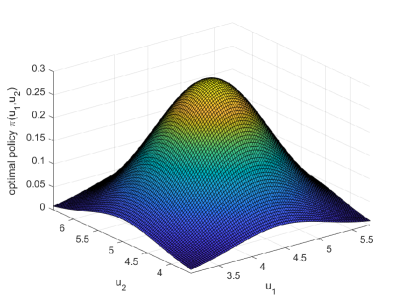
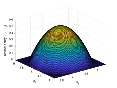
Figure 1: (a) The optimal policy $(u_{1},u_{2})\to\hat{\pi}(u_{1},u_{2})$ with $p=1$. (b): The optimal policy $(u_{1},u_{2})\to\hat{\pi}(u1,u2)$ with $p=2$. The model parameters are set to be $\lambda=1,\leavevmode\nobreak\ \kappa=1,\leavevmode\nobreak\ c=1,\leavevmode\nobreak\ \gamma=1,\leavevmode\nobreak\ t=1,\leavevmode\nobreak\ T=2,\leavevmode\nobreak\ x=5$.

The next remark is concerned with the case when the temperature parameter tends to zero.

Remark 5.4.

When the temperature parameter $\gamma$ goes to $0$, we have $\tilde{\psi}(t)(p-1)\to 0$. It then follows that

$$\int_{\mathds{R}^{2}}(u_{1}^{2}+u_{2}^{2})\pi(u|t,x)du =\frac{\tilde{\psi}(t)(p-1)}{2\kappa(2p-1)}+\frac{(\alpha^{*}(t)x)^{2}}{4\kappa^{2}}-\frac{\tilde{\psi}(t)(p-1)}{\alpha^{*}(t)\lambda(2p-1)}+x^{2}$$

$$\xrightarrow[]{\gamma\to 0}\left(\frac{\alpha^{*}(t)x}{2\kappa}\right)^{2}+x^{2},$$

which yields the convergence of the optimal trading policy to a constant strategy that $(\xi_{t},\eta_{t})\xrightarrow[\gamma\to 0]{L^{2}}\left(\frac{\alpha^{*}(t)x}{2\kappa},x\right)$ for all $(t,x)\in[0,T]\times\mathds{R}$.

Due to the singularity of terminal condition in (5.3), applying q-learning algorithm directly to the primal problem (5.2) may bring great numerical error. Therefore, we provide a parameterization method of the value function and q-function of the auxiliary problem (5.6), which can also help us learn the value function given by (5.2). Let us define some parameters as follows:

$$\theta_{1}^{*}=\kappa(w-\lambda),\quad\theta_{2}^{*}=\kappa(w+\lambda),\quad\theta_{3}^{*}=w,\quad\theta_{4}^{*}=c\kappa,\quad\theta_{5}^{*}=\kappa\lambda,$$

$$\zeta_{1}^{*}=\kappa(w-\lambda),\quad\zeta_{2}^{*}=\kappa(w+\lambda),\quad\zeta_{3}^{*}=w,\quad\zeta_{4}^{*}=c\kappa,\quad\zeta_{5}^{*}=\kappa\lambda\quad\zeta_{6}^{*}=\kappa.$$ (5.11)

Then, we can represent the value function and q-function with these parameters by, for $(t,x,\xi,\eta)\in[0,T]\times\mathds{R}^{3}$,

$$V^{\ell}(t,x) =-\frac{1}{2}\frac{\left(\ell\theta_{1}^{*}+4\theta_{4}^{*}\right)e^{\theta_{3}^{*}(T-t)}+\ell\theta_{2}^{*}-4\theta_{4}^{*}}{\left(\theta_{2}^{*}+\ell\right)e^{\theta_{3}^{*}(T-t)}+\theta_{1}^{*}-\ell}x^{2}+\frac{\gamma}{p-1}(T-t)$$

$$\quad-\frac{p^{2}\gamma^{\frac{1}{p}}}{(2p-1)(p-1)}\int_{t}^{T}\left(\frac{1}{\pi}\sqrt{\frac{\theta_{5}^{*}}{2}\frac{\left(\ell\theta_{1}^{*}+4\theta_{4}^{*}\right)e^{\theta_{3}^{*}(T-t)}+\ell\theta_{2}^{*}-4\theta_{4}^{*}}{\left(\theta_{2}^{*}+\ell\right)e^{\theta_{3}^{*}(T-t)}+\theta_{1}^{*}-\ell}}\right)^{\frac{p-1}{p}}ds,$$

$$q^{\ell}(t,x,\xi,\eta) =-\zeta_{6}^{*}\left(\xi-\frac{1}{2\zeta_{6}^{*}}\frac{\left(\ell\zeta_{1}^{*}+4\zeta_{4}^{*}\right)e^{\zeta_{3}^{*}(T-t)}+\ell\zeta_{2}^{*}-4\zeta_{4}^{*}}{\left(\zeta_{2}^{*}+\ell\right)e^{\zeta_{3}^{*}(T-t)}+\zeta_{1}^{*}-\ell}x\right)^{2}$$

$$\quad-\frac{\zeta_{5}^{*}}{2\zeta_{6}^{*}}\frac{\left(\ell\zeta_{1}^{*}+4\zeta_{4}^{*}\right)e^{\zeta_{3}^{*}(T-t)}+\ell\zeta_{2}^{*}-4\zeta_{4}^{*}}{\left(\zeta_{2}^{*}+\ell\right)e^{\zeta_{3}^{*}(T-t)}+\zeta_{1}^{*}-\ell}(\eta-x)^{2}$$

$$\quad+\frac{p^{2}\gamma^{\frac{1}{p}}}{(p-1)(2p-1)}\left(\frac{1}{\pi}\sqrt{\frac{\zeta_{5}^{*}}{2}\frac{\left(\ell\zeta_{1}^{*}+4\zeta_{4}^{*}\right)e^{\zeta_{3}^{*}(T-t)}+\ell\zeta_{2}^{*}-4\zeta_{4}^{*}}{\left(\zeta_{2}^{*}+\ell\right)e^{\zeta_{3}^{*}(T-t)}+\zeta_{1}^{*}-\ell}}\right)^{\frac{p}{p-1}}-\frac{\gamma}{p-1}.$$

In lieu of Theorem 5.2, we can parameterize the optimal value function and the optimal q-function in the exact form as:

$$J^{\theta}(t,x) =-\frac{1}{2}\frac{\left(\ell\theta_{1}+4\theta_{4}\right)e^{\theta_{3}(T-t)}+\ell\theta_{2}-4\theta_{4}}{\left(\theta_{2}+\ell\right)e^{\theta_{3}(T-t)}+\theta_{1}^{*}-\ell}x^{2}+\frac{\gamma}{p-1}(T-t)$$

$$\qquad-\frac{p^{2}\gamma^{\frac{1}{p}}}{(2p-1)(p-1)}\int_{t}^{T}\left(\frac{1}{\pi}\sqrt{\frac{\theta_{5}}{2}\frac{\left(\ell\theta_{1}+4\theta_{4}\right)e^{\theta_{3}(T-t)}+\ell\theta_{2}-4\theta_{4}}{\left(\theta_{2}+\ell\right)e^{\theta_{3}(T-t)}+\theta_{1}-\ell}}\right)^{\frac{p-1}{p}}ds,$$

$$q^{\zeta}(t,x,\xi,\eta) =-\zeta_{6}\left(\xi-\frac{1}{2\zeta_{6}}\frac{\left(\ell\zeta_{1}+4\zeta_{4}\right)e^{\zeta_{3}(T-t)}+\ell\zeta_{2}-4\zeta_{4}}{\left(\zeta_{2}+\ell\right)e^{\zeta_{3}(T-t)}+\zeta_{1}-\ell}x\right)^{2}$$

$$\qquad-\frac{\zeta_{5}}{2\zeta_{6}}\frac{\left(\ell\zeta_{1}+4\zeta_{4}\right)e^{\zeta_{3}(T-t)}+\ell\zeta_{2}-4\zeta_{4}}{\left(\zeta_{2}+\ell\right)e^{\zeta_{3}(T-t)}+\zeta_{1}-\ell}(\eta-x)^{2}+\tilde{\zeta}(t,x),$$

where $\tilde{\zeta}(t,x)$ is a parameterized function to be determined, $(\theta_{1},\theta_{2},\theta_{3},\theta_{4},\theta_{5})\in\mathds{R}_{+}^{5}$ and $(\zeta_{1},\zeta_{2},\zeta_{3},\zeta_{4},\zeta_{5},\zeta_{6})\in\mathds{R}_{+}^{6}$ are unknown parameters to be learnt. Then, by using the normalizing constraint

$$\int_{U}\left(\frac{p-1}{p\gamma}\right)^{\frac{1}{p-1}}\left(q^{\zeta}(t,x,u)+\psi^{\zeta}(t,x)\right)_{+}^{\frac{1}{p-1}}du=1,$$

we get the following normalizing function $\psi^{\zeta}(t,x)$ given by

$$\psi^{\zeta}(t,x)=\left(\frac{1}{\pi}\sqrt{\frac{\zeta_{5}}{2}\frac{\left(\ell\zeta_{1}+4\zeta_{4}\right)e^{\zeta_{3}(T-t)}+\ell\zeta_{2}-4\zeta_{4}}{\left(\zeta_{2}+\ell\right)e^{\zeta_{3}(T-t)}+\zeta_{1}-\ell}}\right)^{\frac{p-1}{p}}\frac{p}{p-1}\gamma^{\frac{1}{p}}-\tilde{\zeta}(t,x).$$ (5.12)

Furthermore, since the parameterized q-function satisfies

$$\int_{U}[q^{\zeta}(t,x,u)+\gamma l_{p}(\pi^{\zeta}(u|t,x))]\pi^{\zeta}(u|t,x)du=0,$$

we deduce that

$$\tilde{\zeta}(t,x)=\frac{p^{2}\gamma^{\frac{1}{p}}}{(p-1)(2p-1)}\left(\frac{1}{\pi}\sqrt{\frac{\zeta_{5}}{2}\frac{\left(\ell\zeta_{1}+4\zeta_{4}\right)e^{\zeta_{3}(T-t)}+\ell\zeta_{2}-4\zeta_{4}}{\left(\zeta_{2}+\ell\right)e^{\zeta_{3}(T-t)}+\zeta_{1}-\ell}}\right)^{\frac{p}{p-1}}-\frac{\gamma}{p-1}.$$ (5.13)

Then, the parameterized policy $\pi^{\zeta}$ is given by

$$\pi^{\zeta}(\xi,\eta|t,x)=\left(\frac{p-1}{p\gamma}\right)^{\frac{1}{p-1}}\Bigg{(}\left(\frac{1}{\pi}\sqrt{\frac{\zeta_{5}}{2}\frac{\left(\ell\zeta_{1}+4\zeta_{4}\right)e^{\zeta_{3}(T-t)}+\ell\zeta_{2}-4\zeta_{4}}{\left(\zeta_{2}+\ell\right)e^{\zeta_{3}(T-t)}+\zeta_{1}-\ell}}\right)^{\frac{p-1}{p}}\frac{p}{p-1}\gamma^{\frac{1}{p}}$$ (5.14)

$$-\zeta_{6}\left(\xi-\frac{1}{2\zeta_{6}}\frac{\left(\ell\zeta_{1}+4\zeta_{4}\right)e^{\zeta_{3}(T-t)}+\ell\zeta_{2}-4\zeta_{4}}{\left(\zeta_{2}+\ell\right)e^{\zeta_{3}(T-t)}+\zeta_{1}-\ell}x\right)^{2}-\frac{\zeta_{5}}{2\zeta_{6}}\frac{\left(\ell\zeta_{1}+4\zeta_{4}\right)e^{\zeta_{3}(T-t)}+\ell\zeta_{2}-4\zeta_{4}}{\left(\zeta_{2}+\ell\right)e^{\zeta_{3}(T-t)}+\zeta_{1}-\ell}(\eta-x)^{2}\Bigg{)}_{+}^{\frac{1}{p-1}}.$$

Simulator: In what follows, we apply Algorithm 1 with the above parameterized value function and q-function. To generate sample trajectories, we first apply the acceptance-rejection sampling method (c.f. Flury 1990) to generate the control pair $(u^{1}_{t},u^{2}_{t})$ from the q-Gaussian distribution with density function given by (5.14) at time $t$. Then, the control pair $(u^{1}_{t},u^{2}_{t})$ is used to the following simulator

$$X_{t+\Delta t}-X_{t}=-u^{1}_{t}\Delta t-u^{2}_{t}N(\Delta t),$$

where $N(\Delta t)$ is a Poisson random variable with rate $\lambda\Delta t$.

Algorithm Inputs: We set the coefficients of the simulator to $\lambda=0.01,X_{0}=2,T=0.25$, the known parameters as $\gamma=0.01,p=3,c=1,\kappa=1,\ell=10,x=2,T=0.25$, the time step as $dt=0.01$, and the number of iterations as $N=10000$. The learning rates are set as follows:

$$\alpha_{\theta_{1}}(k) =\begin{cases}\displaystyle 0.01,\leavevmode\nobreak\ \text{if }1\leq k\leq 2500,\\ \displaystyle\frac{0.001}{{\rm linspace}_{(1,20,N)}(k)},\leavevmode\nobreak\ \text{if }2500<k\leq N,\end{cases}\leavevmode\nobreak\ \alpha_{\theta_{2}}(k)=\begin{cases}\displaystyle 0.005,\leavevmode\nobreak\ \text{if }1\leq k\leq 4000,\\ \displaystyle\frac{0.005}{{\rm linspace}_{(1,100,N)}(k)},\leavevmode\nobreak\ \text{if }4000<k\leq N,\end{cases}$$

$$\alpha_{\theta_{3}}(k) =\begin{cases}\displaystyle 0.01,\leavevmode\nobreak\ \text{if }1\leq k\leq 4000,\\ \displaystyle\frac{0.005}{{\rm linspace}_{(1,20,N)}(k)},\leavevmode\nobreak\ \text{if }4000<k\leq N,\end{cases}\leavevmode\nobreak\ \alpha_{\theta_{4}}(k)=\begin{cases}\displaystyle 0.03,\leavevmode\nobreak\ \text{if }1\leq k\leq 3000,\\ \displaystyle\frac{0.005}{{\rm linspace}_{(1,20,N)}(k)},\leavevmode\nobreak\ \text{if }3000<k\leq N,\end{cases}$$

$$\alpha_{\theta_{5}}(k) =\begin{cases}\displaystyle 0.05,\leavevmode\nobreak\ \text{if }1\leq k\leq 3000,\\ \displaystyle\frac{0.0005}{{\rm linspace}_{(1,20,N)}(k)},\leavevmode\nobreak\ \text{if }3000<k\leq N,\end{cases}\leavevmode\nobreak\ \alpha_{\zeta_{1}}(k)=\begin{cases}\displaystyle 0.03,\leavevmode\nobreak\ \text{if }1\leq k\leq 3500,\\ \displaystyle\frac{0.00135}{{\rm linspace}_{(1,10,N)}(k)},\leavevmode\nobreak\ \text{if }3500<k\leq N,\end{cases}$$

$$\alpha_{\zeta_{2}}(k) =\begin{cases}\displaystyle 0.1,\leavevmode\nobreak\ \text{if }1\leq k\leq 3500,\\ \displaystyle\frac{0.0002}{{\rm linspace}_{(1,500,N)}(k)},\leavevmode\nobreak\ \text{if }3500<k\leq N,\end{cases}\leavevmode\nobreak\ \alpha_{\zeta_{3}}(k)=\begin{cases}\displaystyle 0.1,\leavevmode\nobreak\ \text{if }1\leq k\leq 2000,\\ \displaystyle 0.002,\leavevmode\nobreak\ \text{if }2000<k\geq 5000,\\ \displaystyle\frac{0.0005}{{\rm linspace}_{(1,20,N)}(k)},\leavevmode\nobreak\ \text{if }k\geq 5000,\end{cases}$$

$$\alpha_{\zeta_{4}}(k) =\begin{cases}\displaystyle 0.005,\leavevmode\nobreak\ \text{if }1\leq k\leq 7000,\\ \displaystyle\frac{0.001}{{\rm linspace}_{(1,100,N)}(k)},\leavevmode\nobreak\ \text{if }7000<k\leq N,\end{cases}\leavevmode\nobreak\ \alpha_{\zeta_{5}}(k)=\begin{cases}\displaystyle 0.006,\leavevmode\nobreak\ \text{if }1\leq k\leq 5000,\\ \displaystyle\frac{0.002}{{\rm linspace}_{(1,10,N)}(k)},\leavevmode\nobreak\ \text{if }5000<k\leq N,\end{cases}$$

$$\alpha_{\zeta_{6}}(k) =\begin{cases}\displaystyle 0.006,\leavevmode\nobreak\ \text{if }1\leq k\leq 5000,\\ \displaystyle\frac{0.002}{{\rm linspace}_{(1,10,N)}(k)},\leavevmode\nobreak\ \text{if }5000<k\leq N,\end{cases}$$

where ${\rm linspace}_{(a,b,n)}(\cdot)$ is the Matlab function that returns a row vector of $n$ points linearly spaced between and including $a$ and $b$ with the spacing between the points being $\frac{b-a}{n-1}$.

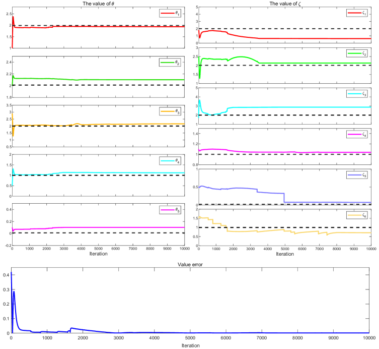
Figure 2: Convergence of the offline q-learning algorithm under a market simulator for the parameters $(\theta_{1},\theta_{2},\theta_{3},\theta_{4},\theta_{5},\zeta_{1},\zeta_{2},\zeta_{3},\zeta_{4},\zeta_{5},\zeta_{6})$. The $x$-axis and $y$-axis of the upper panels show the iteration steps and the learned parameters, respectively. The $x$-axis and $y$-axis of the bottom panel show the iteration steps and the value error, respectively.

Table 1: Parameters used in the simulator.

Parameters	True value	Learnt by Algorithm 1
$(\theta_{1},\theta_{2},\theta_{3},\theta_{4},\theta_{5})$	$(1.99,2.01,2,1,0.01)$	$(1.9362,2.1013,2.1604,1.1215,0.1008)$
$(\zeta_{1},\zeta_{2},\zeta_{3},\zeta_{4},\zeta_{5},\zeta_{6})$	$(1.99,2.01,2,1,0.01,1)$	$(0.6185,2.1372,2.8776,1.0380,0.1008,0.7107)$

We then track the parameters $(\theta_{1},\theta_{2},\theta_{3},\theta_{4},\theta_{5})$, $(\zeta_{1},\zeta_{2},\zeta_{3},\zeta_{4},\zeta_{5},\zeta_{6})$, and the error of the value function throughout the iterative process. Table 1 reports the estimated parameter values and the corresponding value learned by Algorithm 1. Figure 2 plots the convergence behavior of the dark pool trading problem by the offline learning algorithm within the framework of Tsallis entropy. After sufficient iterations, these parameters achieve a convergent state, indicating that they have reached their optimal values. Concurrently, the value error also converges to zero. The convergence of both the model parameters and the value error underscores the effectiveness and robustness of the offline learning algorithm under Tsallis entropy in accurately capturing the jump-diffusion dynamics of the system.

5.2 An example of non-LQ jump-diffusion control

In this section, we consider a class of non-LQ control problems with jumps in which we can obtain the closed-form solution with the choice of the Tsallis entropy index $p=2$. More precisely, let $u=(u_{t})_{t\in[0,T]}=(\xi_{t},\eta_{t})_{t\in[0,T]}\in{\cal U}$ be the corresponding control strategy taking values on $U=\mathds{R}^{2}$. Let us consider the associated controlled state process under the control $u=(\xi,\eta)\in{\cal U}$, which is described as, for $s\in(t,T]$ with $t\in[0,T]$,

$$\frac{dX_{s}^{u}}{X_{s-}^{u}} =\xi_{s-}\mu_{1}ds+\eta_{s-}\mu_{2}ds+\sigma dW_{s}-\nu dN_{s},\quad X_{t}^{u}=x>0,$$ (5.15)

where the parameters $\mu_{1},\mu_{2}\in\mathds{R}$, $\sigma>0$ and $\nu<1$. We use $\mu_{1},\mu_{2}\geq 0$ to denote the rate charged by a hedger when he lends money to the two kinds of repo market and implements his short-selling position (see also Bichuch et al. 2018). Then, the dynamics (5.15) describes the cash flow controlled by the lending strategy $(\xi,\eta)$. The value function with the state process (5.15) is specified as follows:

$$v(t,x)=\sup_{u=(\xi,\eta)\in{\cal U}}\mathbb{E}\left[U(X_{T}^{u})-\int_{t}^{T}\left\{A\xi_{s}^{2}(X_{s}^{u})^{2h}+B\eta_{s}^{2}(X_{s}^{u})^{2h}\right\}ds\right].$$ (5.16)

Here $U(x)=\frac{x^{h}}{h}$ is the standard power utility for $x>0$, $0<h<1$, and $A,B>0$ are the cost parameters.

The exploratory formulation for the problem (5.15)-(5.16) under Tsallis entropy is given by, for $(t,x)\in[t,T]\times\mathds{R}_{+}$,

$$V(t,x) =\sup_{\pi\in\Pi}\mathbb{E}\left[\frac{(X_{T}^{\pi})^{h}}{h}+\int_{t}^{T}\int_{\mathds{R}^{2}}\left\{-Au_{1}^{2}(X_{s}^{\pi})^{2h}-Bu_{2}^{2}(X_{s}^{\pi})^{2h}+\gamma l_{p}(\pi_{s}(u))\right\}\pi_{s}(u)duds\right],$$

$${\rm s.t.}\leavevmode\nobreak\ X_{s}^{\pi} =x+\int_{t}^{s}\int_{\mathds{R}^{2}}(u_{1}\mu_{1}+u_{2}\mu_{2})X_{v}^{\pi}\pi_{v}(du)dv+\int_{t}^{s}\sigma X_{v}^{\pi}dW_{v}$$ (5.17)

$$\quad-\int_{0}^{t}\nu X_{v-}^{\pi}dN_{v},\leavevmode\nobreak\ \forall s\in[t,T].$$

Then, the exploratory HJB equation satisfied by $V(t,x)$ is formally written as

$$0 =V_{t}+\frac{\sigma^{2}}{2}x^{2}V_{xx}+\lambda(V(t,(1-\nu)x)-V(t,x))$$

$$\quad+\sup_{\pi_{t}\in\mathcal{P}(U)}\bigg{\{}xV_{x}\left(\mu_{1}\int_{U}u_{1}\pi(u|t,x)du+\mu_{2}\int_{\mathds{R}^{2}}u_{2}\pi(u|t,x)du\right)$$

$$\quad-Ax^{2h}\int_{\mathds{R}^{2}}u_{1}^{2}\pi(u|t,x)du-Bx^{2h}\int_{\mathds{R}^{2}}u_{2}^{2}\pi(u|t,x)du+\gamma\int_{\mathds{R}^{2}}l_{p}(\pi(u|t,x))\pi(u|t,x)du\bigg{\}}$$ (5.18)

with terminal condition $V(T,x)=\frac{x^{h}}{h}$ for all $x\in\mathds{R}_{+}$. To enforce the constraints $\int_{U}\pi(u|t,x)du=1$ and $\pi(u|t,x)\geq 0$ for $(t,x,u)\in[0,T]\times\mathds{R}_{+}\times U$, we introduce the Lagrangian given by

$${\cal L}(t,x,\pi,\psi,\zeta) :=xV_{x}\left(\mu_{1}\int_{U}u_{1}\pi(u|t,x)du+\mu_{2}\int_{U}u_{2}\pi(u|t,x)du\right)$$

$$\quad-Ax^{2h}\int_{U}u_{1}^{2}\pi(u|t,x)du-Bx^{2h}\int_{U}u_{2}^{2}\pi(u|t,x)du$$

$$\quad+\frac{\gamma}{p-1}\int_{U}(\pi(u|t,x)-\pi^{p}(u|t,x))du+\psi(t,x)\left(\int_{U}\pi(u|t,x)du-1\right)$$

$$\quad+\int_{U}\zeta(t,x,u)\pi(u|t,x)du,$$

where $\psi(t,x)$ is a function of $(t,x)\in[0,T]\times\mathds{R}_{+}$, and $\zeta(t,x,u)$ is a function of $(t,x,u)\in[0,T]\times\mathds{R}_{+}\times U$. It follows from the first-order condition that

$$\widehat{\pi}(u|t,x)=\left(\frac{p-1}{\gamma p}\right)^{\frac{1}{p-1}}\left(\psi(t,x)+\mu_{1}xV_{x}u_{1}-Ax^{2h}u_{1}^{2}+\mu_{2}xV_{x}u_{2}-Bx^{2h}u_{2}^{2}+\frac{\gamma}{p-1}\right)_{+}$$ (5.19)

with the multiplier $\zeta(t,x,u)$ given by

$$\zeta(t,x,u)=\left(-\frac{\gamma}{p-1}-\mu_{1}xV_{x}u_{1}+Ax^{2h}u_{1}^{2}-\mu_{2}xV_{x}u_{2}+Bx^{2h}u_{2}^{2}-\psi(t,x)\right)_{+},\quad p>1,$$

We next derive the closed-form solution to the exploratory HJB equation (5.2) for $p=2$. We guess that the exploratory HJB equation (5.2) has the solution in the form of

$$V(t,x)=\alpha^{*}(t)\frac{x^{h}}{h}+\beta^{*}(t),\quad\forall(t,x)\in[0,T]\times\mathds{R}_{+}.$$ (5.20)

Plugging this solution form into (5.19), we obtain

$$\widehat{\pi}(u|t,x) =\left(\frac{(p-1)\tilde{\psi}(t,x)}{\gamma p}\right)^{\frac{1}{p-1}}\left(1-\frac{Ax^{2h}}{\tilde{\psi}(t,x)}\left(u_{1}-Y_{1}(t,x)\right)^{2}-\frac{Bx^{2h}}{\tilde{\psi}(t,x)}\left(u_{2}-Y_{2}(t,x)\right)^{2}\right)_{+}^{\frac{1}{p-1}}$$

with $\tilde{\psi}(t,x)=\psi(t,x)+\frac{\gamma}{p-1}+Y_{1}^{2}(t,x)+Y_{2}^{2}(t,x)$, which is assumed to be greater than zero and will be verified later. Here, we define $Y_{1}(t,x):=\frac{\mu_{1}\alpha^{*}(t)}{2Ax^{h}}$ and $Y_{2}(t,x):=\frac{\mu_{2}\alpha^{*}(t)}{2Bx^{h}}$. Using the constraint $\int_{U}\pi(u|x)du=1$, we have

$$1 =\left(\frac{(p-1)\tilde{\psi}(t,x)}{\gamma p}\right)^{\frac{1}{p-1}}\int_{\mathds{R}^{2}}\left(1-\frac{Ax^{2h}}{\tilde{\psi}(t,x)}\left(u_{1}-Y_{1}(t,x)\right)^{2}-\frac{Bx^{2h}}{\tilde{\psi}(t,x)}\left(u_{2}-Y_{2}(t,x)\right)^{2}\right)_{+}^{\frac{1}{p-1}}du$$

$$=\left(\frac{(p-1)\tilde{\psi}(t,x)}{p}\right)^{\frac{p}{p-1}}\frac{\pi}{\gamma^{\frac{1}{p-1}}}\frac{1}{\sqrt{AB}x^{2h}}.$$

This yields that, for all $(t,x)\in[0,T]\times\mathds{R}_{+}$,

$$\tilde{\psi}(t,x)=\left(\frac{\sqrt{AB}x^{2h}}{\pi}\right)^{\frac{p-1}{p}}\frac{p}{p-1}\gamma^{\frac{1}{p}}.$$ (5.21)

As $p>1$, it follows from (5.21) that $\tilde{\psi}(t,x)$ is positive. In order to determine the coefficients $\alpha^{*}(t)$ and $\beta^{*}(t)$ in (5.20), we first compute the following moments of the optimal policy that

$$\int_{\mathds{R}^{2}}u_{1}^{k}\widehat{\pi}(u|t,x)du=\begin{cases}\displaystyle\frac{\mu_{1}}{2Ax^{h}}\alpha^{*}(t),\quad k=1,\\[11.99998pt] \displaystyle\frac{(p-1)\tilde{\psi}(t,x)}{2A(2p-1)x^{2h}}+\left(\frac{\mu_{1}}{2Ax^{h}}\alpha^{*}(t)\right)^{2},\quad k=2,\end{cases}$$

and

$$\int_{\mathds{R}^{2}}u_{2}^{k}\widehat{\pi}(u|t,x)du=\begin{cases}\displaystyle\frac{\mu_{2}}{2Bx^{h}}\alpha^{*}(t),\quad k=1,\\[11.99998pt] \displaystyle\frac{(p-1)\tilde{\psi}(t,x)}{2B(2p-1)x^{2h}}+\left(\frac{\mu_{2}}{2Bx^{h}}\alpha^{*}(t)\right)^{2},\quad k=2.\end{cases}$$

Moreover, it holds that

$$\int_{\mathds{R}^{2}}\frac{1}{p-1}\left(\widehat{\pi}(u|t,x)-\widehat{\pi}(u|t,x)^{p}\right)du=\frac{1}{p-1}-\int_{\mathds{R}^{2}}\frac{\widehat{\pi}(u|t,x)^{p}}{p-1}du=\frac{1}{p-1}-\frac{\tilde{\psi}(t,x)}{\gamma(2p-1)}.$$ (5.22)

Substituting the above terms into Eq. (5.2), we derive

$$0 =\frac{d\alpha^{*}(t)}{dt}\frac{x^{h}}{h}+\frac{d\beta^{*}(t)}{dt}+\frac{\sigma^{2}}{2}(h-1)\alpha^{*}(t)x^{h}+\frac{\mu_{1}^{2}}{4A}(\alpha^{*}(t))^{2}+\frac{\mu_{2}^{2}}{4B}(\alpha^{*}(t))^{2}+\lambda\frac{(1-\nu)^{h}-1}{h}\alpha^{*}(t)x^{h}$$

$$\quad-\frac{p\tilde{\psi}}{2p-1}+\frac{\gamma}{p-1}$$

$$=\frac{d\alpha^{*}(t)}{dt}\frac{x^{h}}{h}+\frac{d\beta(t)}{dt}+\frac{\sigma^{2}}{2}(h-1)\alpha^{*}(t)x^{h}+\frac{\mu_{1}^{2}}{4A}(\alpha^{*}(t))^{2}+\frac{\mu_{2}^{2}}{4B}(\alpha^{*}(t))^{2}+\lambda\frac{(1-\nu)^{h}-1}{h}\alpha^{*}(t)x^{h}$$

$$\quad-\frac{p}{2p-1}\left(\frac{\sqrt{AB}x^{2h}}{\pi}\right)^{\frac{p-1}{p}}\frac{p}{p-1}\gamma^{\frac{1}{p}}+\frac{\gamma}{p-1}.$$ (5.23)

Then, we have the following explicit solution for the exploratory problem (5.2).

Proposition 5.5.

For the Tsallis entropy with $p=2$, the RL problem (5.2) has the following explicit value function given by

$$V(t,x)=\frac{\alpha^{*}(t)}{h}x^{h}+\beta^{*}(t),\quad\forall(t,x)\in[0,T]\times\mathds{R}_{+},$$ (5.24)

where the coefficients $\alpha^{*}(t)$ and $\beta^{*}(t)$ for $t\in[0,T]$ are given by

$$\begin{cases}\displaystyle\alpha^{*}(t)=e^{\left(\frac{\sigma^{2}}{2}(h-1)h+\lambda((1-\nu)^{h}-1)\right)(T-t)},\\[10.00002pt] \displaystyle\beta^{*}(t)=\left(\frac{\mu_{1}^{2}}{4A}+\frac{\mu_{2}^{2}}{4B}\right)\frac{e^{2\left(\frac{\sigma^{2}}{2}(h-1)h+\lambda((1-\nu)^{h}-1)\right)(T-t)}-1}{2\left(\frac{\sigma^{2}}{2}(h-1)h+\lambda((1-\nu)^{h}-1)\right)}\\[6.00006pt] \displaystyle\qquad\qquad-\left(\frac{4}{3}\sqrt{\frac{\gamma}{\pi}}(AB)^{\frac{1}{4}}-{\gamma}\right)(T-t).\end{cases}$$ (5.25)

The optimal policy for problem (5.2) is given by, for $(t,x)\in[0,T]\times\mathds{R}_{+}$ and $u=(u_{1},u_{2})\in U=\mathds{R}^{2}$,

$$\widehat{\pi}(u|t,x) =\frac{1}{2\gamma}\left\{2(AB)^{\frac{1}{4}}\sqrt{\frac{\gamma}{\pi}}x^{h}-Ax^{2h}\left(u_{1}-\frac{\mu_{1}\alpha^{*}(t)}{2Ax^{h}}\right)^{2}-Bx^{2h}\left(u_{2}-\frac{\mu_{2}\alpha^{*}(t)}{2Bx^{h}}\right)^{2}\right\}_{+}.$$ (5.26)

Proof.

For $p=2$, Eq. (5.2) yields that

$$0 =(\alpha^{*}(t))^{\prime}\frac{x^{h}}{h}+(\beta^{*}(t))^{\prime}+\frac{\sigma^{2}}{2}(h-1)\alpha^{*}(t)x^{h}+\lambda\frac{(1-\nu)^{h}-1}{h}\alpha^{*}(t)x^{h}$$

$$\quad+\frac{\mu_{1}^{2}}{4A}(\alpha^{*}(t))^{2}+\frac{\mu_{2}^{2}}{4B}(\alpha^{*}(t))^{2}-\frac{4}{3}\left(\frac{{(AB)}^{\frac{1}{4}}x^{h}}{\sqrt{\pi}}\right)\sqrt{\gamma}+\gamma.$$

Then, it holds that

$$\begin{cases}\displaystyle\frac{(\alpha^{*}(t))^{\prime}}{h}+\left(\frac{\sigma^{2}}{2}(h-1)+\lambda\frac{(1-\nu)^{h}-1}{h}\right)\alpha^{*}(t)=0,\leavevmode\nobreak\ \alpha^{*}(T)=1,\\[8.00003pt] \displaystyle(\beta^{*}(t))^{\prime}+\left(\frac{\mu_{1}^{2}}{4A}+\frac{\mu_{2}^{2}}{4B}\right)(\alpha^{*}(t))^{2}-\frac{4}{3}\left(\frac{{(AB)}^{\frac{1}{4}}}{\sqrt{\pi}}\right)\sqrt{\gamma}+\gamma=0,\leavevmode\nobreak\ \beta^{*}(T)=0.\end{cases}$$

Furthermore, we derive by solving the above equation that

$$\begin{cases}\displaystyle\alpha^{*}(t)=e^{\left(\frac{\sigma^{2}}{2}(h-1)h+\lambda((1-\nu)^{h}-1)\right)(T-t)},\\[8.00003pt] \displaystyle\beta^{*}(t)=\left(\frac{\mu_{1}^{2}}{4A}+\frac{\mu_{2}^{2}}{4B}\right)\frac{e^{2\left(\frac{\sigma^{2}}{2}(h-1)h+\lambda((1-\nu)^{h}-1)\right)(T-t)}-1}{2\left(\frac{\sigma^{2}}{2}(h-1)h+\lambda((1-\nu)^{h}-1)\right)}-\left(\frac{4}{3}\sqrt{\frac{q}{\pi}}(AB)^{\frac{1}{4}}-q\right)(T-t).\end{cases}$$

Similar to the proof of Theorem 5.2, it is not difficult to verify that the value function (5.24) is optimal for the exploratory problem (5.2) by using Itô’s formula:

$$dV(t,\hat{X}_{t}) =V_{t}(t,\hat{X}_{t})dt$$

$$\quad+V_{x}(t,\hat{X}_{t})d\hat{X}_{t}^{c}+\frac{\sigma^{2}}{2}V_{xx}(t,\hat{X}_{t})dt+\int_{U}\lambda(V(t,\hat{X}_{t}-u_{2})-V(t,\hat{X}_{t}))\hat{\pi}(du)dt+M_{t},$$

where $\hat{X}=(\hat{X})_{t\in[0,T]}$ is the state process under the policy $\hat{\pi}$, and $M=(M_{t})_{t\in[0,T]}$ is a (local) martingale. ∎

Remark 5.6.

Notably, the explicit results in Proposition 5.5 are exclusive to the special Tsallis entropy when $p=2$. This distinction is crucial, as it delineates a limitation in Shannon entropy’s applicability, given its implicit assumption of $p=1$. Consequently, endeavors utilizing Shannon entropy would fail to adequately explore this particular Non-LQ problem (5.16). Furthermore, the optimal policy given by (5.26) is also a two-dimensional q-Gaussian distribution with a compact support set (see Figure 3). In fact, for $(t,x)\in[0,T]\times(0,+\infty)$, we have

$$u_{1} \in\left[\frac{\mu_{1}\alpha^{*}(t)}{2Ax^{h}}-\sqrt{\frac{2B^{\frac{1}{4}}}{A^{\frac{3}{4}}x^{h}}\sqrt{\frac{\gamma}{\pi}}},\frac{\mu_{1}\alpha^{*}(t)}{2Ax^{h}}+\sqrt{\frac{2B^{\frac{1}{4}}}{A^{\frac{3}{4}}x^{h}}\sqrt{\frac{\gamma}{\pi}}}\right],$$

$$u_{2} \in\left[\frac{\mu_{2}\alpha^{*}(t)}{2Bx^{h}}-\sqrt{\frac{2A^{\frac{1}{4}}}{B^{\frac{3}{4}}x^{h}}\sqrt{\frac{\gamma}{\pi}}},\frac{\mu_{2}\alpha^{*}(t)}{2Bx^{h}}+\sqrt{\frac{2A^{\frac{1}{4}}}{B^{\frac{3}{4}}x^{h}}\sqrt{\frac{\gamma}{\pi}}}\right].$$

Here, the function $t\mapsto\alpha^{*}(t)$ is given by (5.25).

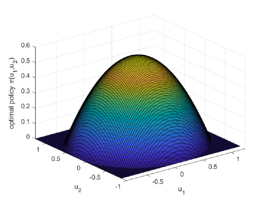
Figure 3: The optimal policy $(u_{1},u_{2})\to\widehat{\pi}(u_{1},u_{2})$. The model parameters are set to be $\lambda=1,\leavevmode\nobreak\ \sigma=1,\leavevmode\nobreak\ \nu=0.5,\leavevmode\nobreak\ A=B=1,\leavevmode\nobreak\ \mu_{1}=\mu_{2}=0.5,\leavevmode\nobreak\ h=1.5,\leavevmode\nobreak\ \gamma=1,\leavevmode\nobreak\ t=1,\leavevmode\nobreak\ T=2,\leavevmode\nobreak\ x=1$.

Remark 5.7.

When the temperature parameter $\gamma$ goes to $0$, we have $\tilde{\psi}(t,x)(p-1)\to 0$. Then, it holds that

$$\int_{\mathds{R}^{2}}(u_{1}^{2}+u_{2}^{2})\pi(u|t,x)du =\frac{(p-1)\tilde{\psi}(t,x)}{2A(2p-1)x^{2h}}+\left(\frac{\mu_{1}}{2Ax^{h}}\alpha^{*}(t)\right)^{2}+\frac{(p-1)\tilde{\psi}(t,x)}{2B(2p-1)x^{2h}}+\left(\frac{\mu_{2}}{2Bx^{h}}\alpha^{*}(t)\right)^{2}$$

$$\xrightarrow[]{\gamma\to 0}\left(\frac{\mu_{1}}{2Ax^{h}}\alpha^{*}(t)\right)^{2}+\left(\frac{\mu_{2}}{2Bx^{h}}\alpha^{*}(t)\right)^{2}.$$

This implies the convergence of the borrowing and lending policy to a constant strategy that $(\xi_{t},\eta_{t})\xrightarrow[\gamma\to 0]{L^{2}}\left(\frac{\mu_{1}}{2Ax^{h}}\alpha^{*}(t),\frac{\mu_{2}}{2Bx^{h}}\alpha^{*}(t)\right)$ for $(t,x)\in[0,T]\times\mathds{R}_{+}$.

Let us propose the following parameters as follows:

$$\begin{cases}\displaystyle\theta_{1}^{*}=\frac{\sigma^{2}}{2}(h-1)h+\lambda((1-\nu)^{h}-1),\\[8.00003pt] \displaystyle\theta_{2}^{*}=\left(\frac{\mu_{1}^{2}}{4A}+\frac{\mu_{2}^{2}}{4B}\right)\frac{1}{2\left(\frac{\sigma^{2}}{2}(h-1)h+\lambda((1-\nu)^{h}-1)\right)},\\[8.00003pt] \displaystyle\theta_{3}^{*}=\frac{4}{3}\sqrt{\frac{1}{\pi}}(AB)^{\frac{1}{4}},\end{cases}$$ (5.27)

and

$$\zeta_{1}^{*}=\frac{\sigma^{2}}{2}(h-1)h+\lambda((1-\nu)^{h}-1),\quad\zeta_{2}^{*}=A,\quad\zeta_{3}^{*}=B,\quad\zeta_{4}^{*}=\frac{\mu_{1}}{2A},\quad\zeta_{5}^{*}=\frac{\mu_{2}}{2B}.$$ (5.28)

Thus, we can represent the value function and q-function with these parameters by, for $(t,x,u_{1},u_{2})\in[0,T]\times\mathds{R}_{+}\times\mathds{R}^{2}$

$$V(t,x) =\frac{e^{\theta_{1}^{*}(T-t)}}{h}x^{h}+\theta_{2}^{*}\left(e^{2\theta_{1}^{*}(T-t)}-1\right)-(\theta_{3}^{*}\sqrt{\gamma}-\gamma)(T-t),$$

$$q(t,x,u_{1},u_{2}) =-\zeta_{2}^{*}x^{2h}\left(u_{1}-\frac{\zeta_{4}^{*}e^{\zeta_{1}^{*}(T-t)}}{x^{h}}\right)^{2}-\zeta_{3}^{*}x^{2h}\left(u_{2}-\frac{\zeta_{5}^{*}e^{\zeta_{1}^{*}(T-t)}}{x^{h}}\right)^{2}+\frac{4}{3}\sqrt{\frac{\gamma}{\pi}}(\zeta_{2}^{*}\zeta_{3}^{*})^{\frac{1}{4}}-\gamma.$$

Building upon Theorem 5.2, we can parameterize the optimal value function and the optimal q-function in the exact form as:

$$J^{\theta}(t,x) =\frac{e^{\theta_{1}(T-t)}}{h}x^{h}+\theta_{2}\left(e^{2\theta_{1}(T-t)}-1\right)-(\theta_{3}\sqrt{\gamma}-\gamma)(T-t),$$

$$q^{\zeta}(t,x,\xi,\eta) =-\zeta_{2}x^{2h}\left(u_{1}-\frac{\zeta_{4}e^{\zeta_{1}(T-t)}}{x^{h}}\right)^{2}-\zeta_{3}x^{2h}\left(u_{2}-\frac{\zeta_{5}e^{\zeta_{1}(T-t)}}{x^{h}}\right)^{2}+\tilde{\zeta}(t,x),$$

where $\tilde{\zeta}(t,x)$ is a parameterized function to be determined, $(\theta_{1},\theta_{2},\theta_{3})\in\mathds{R}^{3}$ and $(\zeta_{1},\zeta_{2},\zeta_{3},\zeta_{4},\zeta_{5})\in\mathds{R}^{5}$ are unknown parameters to be learnt. Then, by using the normalizing constraint

$$\int_{U}\frac{1}{2\gamma}\left(q^{\zeta}(t,x,u)+\psi^{\zeta}(t,x)\right)_{+}du=1,$$

we get the normalizing function $\psi^{\zeta}(t,x)$ given by

$$\psi^{\zeta}(t,x)=2(\zeta_{2}\zeta_{3})^{\frac{1}{4}}\sqrt{\frac{\gamma}{\pi}}-\tilde{\zeta}(t,x).$$ (5.29)

Moreover, note that the parameterized q-function is required to satisfy

$$\int_{U}[q^{\zeta}(t,x,u)+\gamma l_{2}(\pi^{\zeta}(u|t,x))]\pi^{\zeta}(u|t,x)du=0,$$

we deduce that

$$\tilde{\zeta}(t,x)=\frac{4}{3}\sqrt{\frac{\gamma}{\pi}}(\zeta_{2}\zeta_{3})^{\frac{1}{4}}-\gamma.$$

As a consequence, the parameterized policy $\pi^{\zeta}$ is given by

$$\pi^{\zeta}(u_{1},u_{2}|t,x)$$

$$\quad=\frac{1}{2\gamma}\left(2(\zeta_{2}\zeta_{3})^{\frac{1}{4}}\sqrt{\frac{\gamma}{\pi}}x^{h}-\zeta_{2}x^{2h}\left(u_{1}-\frac{\zeta_{4}e^{\zeta_{1}(T-t)}}{x^{h}}\right)^{2}-\zeta_{3}x^{2h}\left(u_{2}-\frac{\zeta_{5}e^{\zeta_{1}(T-t)}}{x^{h}}\right)^{2}\right)_{+}.$$

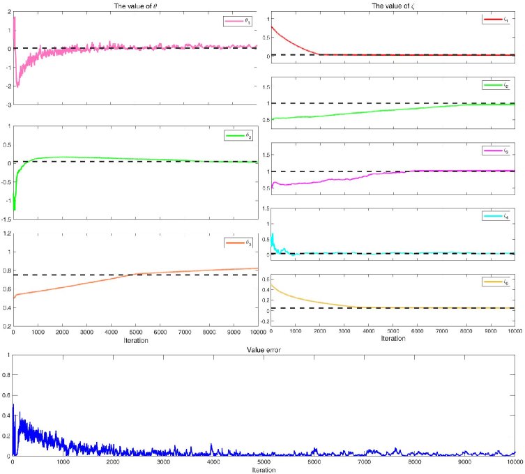
Figure 4: Convergence of the offline q-learning algorithm under a market simulator for the parameters $(\theta_{1},\theta_{2},\theta_{3},\zeta_{1},\zeta_{2},\zeta_{3},\zeta_{4},\zeta_{5})$. The $x$-axis and $y$-axis of the upper panel show the iteration steps and the learned parameters, respectively. The $x$-axis and $y$-axis of the bottom panel show the iteration steps and the value error, respectively.

Simulator: With the above parameterized value function and q-function, we next apply the Algorithm 1. We use the acceptance-rejection sampling method to generate the control pair $(u^{1}_{t},u^{2}_{t})$ from the q-Gaussian distribution with density function given by (5.14) at time $t$. Then the control pair $(u^{1}_{t},u^{2}_{t})$ is used to generate sample trajectories through the following simulator

$$X_{t+\Delta t}-X_{t}=(\mu_{1}u^{1}_{t}+\mu_{2}u_{2})X_{t}\Delta t+\sigma X_{t}W(\Delta t)-\nu X_{t}N(\Delta t),$$

where $N(\Delta t)$ is a Poisson random variable with rate $\lambda\Delta t$, $W(\Delta)$ is a random variable obeying normal distribution ${\cal N}(0,\Delta t)$.

Algorithm Inputs: We set the coefficients of the simulator to $\lambda=0.01,\mu_{1}=0.08,\mu_{2}=0.1,\sigma=0.2,\nu=0.05,X_{0}=2,T=0.5$, the known parameters as $\gamma=0.01,p=2,A=1,B=1,h=2,x=2,T=0.5$, the time step as $dt=0.01$, and the number of iterations as $N=10000$. The learning rates are set as follows:

$$\alpha_{\theta_{1}}(k) =\frac{0.3}{{\rm linspace}_{(1,20,N)}(k)},\leavevmode\nobreak\ \leavevmode\nobreak\ 1\leq k\leq N,\leavevmode\nobreak\ \leavevmode\nobreak\ \leavevmode\nobreak\ \leavevmode\nobreak\ \leavevmode\nobreak\ \leavevmode\nobreak\ \leavevmode\nobreak\ \leavevmode\nobreak\ \leavevmode\nobreak\ \leavevmode\nobreak\ \leavevmode\nobreak\ \leavevmode\nobreak\ \leavevmode\nobreak\ \leavevmode\nobreak\ \leavevmode\nobreak\ \alpha_{\theta_{2}}(k)=\begin{cases}\displaystyle\frac{0.1}{{\rm linspace}_{(1,100,N)}(k)},\leavevmode\nobreak\ \text{if }1\leq k\leq 4000,\\ \displaystyle 0.0025,\leavevmode\nobreak\ \text{if }4000<k\leq 8000,\\ \displaystyle 0.0005,\leavevmode\nobreak\ \text{if }8000<k\leq N,\end{cases}$$

$$\alpha_{\theta_{3}}(k) =\begin{cases}\displaystyle 0.015,\leavevmode\nobreak\ \text{if }1\leq k\leq 4000,\\ \displaystyle\frac{0.05}{{\rm linspace}_{(1,20,N)}(k)},\leavevmode\nobreak\ \text{if }4000<k\leq N,\end{cases}\leavevmode\nobreak\ \leavevmode\nobreak\ \leavevmode\nobreak\ \alpha_{\zeta_{1}}(k)=\begin{cases}\displaystyle 0.022,\leavevmode\nobreak\ \text{if }1\leq k\leq 2000,\\ \displaystyle\frac{0.005}{{\rm linspace}_{(1,25,N)}(k)},\leavevmode\nobreak\ \text{if }2000<k\leq N,\end{cases}$$

$$\alpha_{\zeta_{2}}(k) =\begin{cases}\displaystyle 0.005,\leavevmode\nobreak\ \text{if }1\leq k\leq 8000,\\ \displaystyle\frac{0.005}{{\rm linspace}_{(1,20,N)}(k)},\leavevmode\nobreak\ \text{if }8000<k\leq N,\end{cases}\leavevmode\nobreak\ \leavevmode\nobreak\ \leavevmode\nobreak\ \alpha_{\zeta_{3}}(k)=\begin{cases}\displaystyle 0.02,\leavevmode\nobreak\ \text{if }1\leq k\leq 6000,\\ \displaystyle\frac{0.06}{{\rm linspace}_{(1,600,N)}(k)},\leavevmode\nobreak\ \text{if }k\geq 5000,\end{cases}$$

$$\alpha_{\zeta_{4}}(k) =\frac{0.2}{{\rm linspace}_{(1,100,N)}(k)},\leavevmode\nobreak\ \leavevmode\nobreak\ 1\leq k\leq N,\leavevmode\nobreak\ \leavevmode\nobreak\ \leavevmode\nobreak\ \leavevmode\nobreak\ \leavevmode\nobreak\ \leavevmode\nobreak\ \leavevmode\nobreak\ \leavevmode\nobreak\ \leavevmode\nobreak\ \leavevmode\nobreak\ \leavevmode\nobreak\ \leavevmode\nobreak\ \leavevmode\nobreak\ \leavevmode\nobreak\ \alpha_{\zeta_{5}}(k)=\begin{cases}\displaystyle\frac{0.002}{{\rm linspace}_{(1,30,N)}(k)},\leavevmode\nobreak\ \text{if }1\leq k\leq 3500,\\ \displaystyle\frac{0.0001}{{\rm linspace}_{(1,50,6500)}(k)},\leavevmode\nobreak\ \text{if }5000<k\leq N.\end{cases}$$

Table 2: Parameters used in the simulator.

Parameters	True value	Learnt by Algorithm 1
$(\theta_{1},\theta_{2},\theta_{3})$	$(0.0390,0.0525,0.7523)$	$(0.0657,0.0508,0.8102)$
$(\zeta_{1},\zeta_{2},\zeta_{3},\zeta_{4},\zeta_{5})$	$(0.0390,1,1,0.04,0.05)$	$(0.0312,0.9628,1.0205,0.0560,0.0516)$

We then track the parameters $(\theta_{1},\theta_{2},\theta_{3})$, $(\zeta_{1},\zeta_{2},\zeta_{3},\zeta_{4},\zeta_{5})$, and the error of the value function throughout the iterative process. Table 2 reports the estimated parameter values and the corresponding value learned by Algorithm 1. After sufficient iterations, it can be seen from Figure 4 that the iterations of parameters exhibit good convergence, and the value error converges to zero, illustrating the satisfactory performance of the proposed q-learning algorithm with the Tsallis entropy for solving this non-LQ example in the jump-diffusion model.

Acknowledgement L. Bo and Y. Huang are supported by Natural Science Basic Research Program of Shaanxi (No. 2023-JC-JQ-05), Shaanxi Fundamental Science Research Project for Mathematics and Physics (No. 23JSZ010) and Fundamental Research Funds for the Central Universities (No. 20199235177). X. Yu is supported by the Hong Kong RGC General Research Fund (GRF) under grant no. 15211524 and the Hong Kong Polytechnic University research grant under no. P0045654.

References

- Benazzoli et al. (2020) Benazzoli C, Campi L, Di Persio L (2020) Mean field games with controlled jump–diffusion dynamics: Existence results and an illiquid interbank market model. Stochastic Processes and their Applications 130(11):6927–6964.
- Bichuch et al. (2018) Bichuch M, Capponi A, Sturm S (2018) Arbitrage-free XVA. Mathematical Finance 28(2):582–620.
- Bo et al. (2023) Bo L, Huang Y, Yu X (2023) On optimal tracking portfolio in incomplete markets: The classical control and the reinforcement learning approaches. Preprint, available at arXiv:2311.14318 .
- Dai et al. (2023) Dai M, Dong Y, Jia Y, Zhou XY (2023) Learning merton’s strategies in an incomplete market: Recursive entropy regularization and biased gaussian exploration. Preprint, available at arXiv:2312.11797 .
- Donnelly and Jaimungal (2024) Donnelly R, Jaimungal S (2024) Exploratory control with tsallis entropy for latent factor models. SIAM Journal on Financial Mathematics 15(1):26–53.
- Flury (1990) Flury BD (1990) Acceptance–rejection sampling made easy. SIAM Review 32(3):474–476.
- Gao et al. (2024) Gao X, Li L, Zhou XY (2024) Reinforcement learning for jump-diffusions. Preprint, available at arXiv:2405.16449 .
- Giegrich et al. (2024) Giegrich M, Reisinger C, Zhang Y (2024) Convergence of policy gradient methods for finite-horizon exploratory linear-quadratic control problems. SIAM Journal on Control and Optimization 62(2):1060–1092.
- Han et al. (2023) Han X, Wang R, Zhou XY (2023) Choquet regularization for continuous-time reinforcement learning. SIAM Journal on Control and Optimization 61(5):2777–2801.
- Jia and Zhou (2022a) Jia Y, Zhou XY (2022a) Policy evaluation and temporal-difference learning in continuous time and space: A martingale approach. Journal of Machine Learning Research 23(154):1–55.
- Jia and Zhou (2022b) Jia Y, Zhou XY (2022b) Policy gradient and actor-critic learning in continuous time and space: Theory and algorithms. Journal of Machine Learning Research 23(275):1–50.
- Jia and Zhou (2023) Jia Y, Zhou XY (2023) q-learning in continuous time. Journal of Machine Learning Research 24(161):1–61.
- Kratz and Schöneborn (2014) Kratz P, Schöneborn T (2014) Optimal liquidation in dark pools. Quantitative Finance 14(9):1519–1539.
- Kratz and Schöneborn (2015) Kratz P, Schöneborn T (2015) Portfolio liquidation in dark pools in continuous time. Mathematical Finance 25(3):496–544.
- Lee et al. (2018) Lee K, Choi S, Oh S (2018) Sparse markov decision processes with causal sparse tsallis entropy regularization for reinforcement learning. IEEE Robotics and Automation Letters 3(3):1466–1473.
- Lee et al. (2019) Lee K, Kim S, Lim S, Choi S, Oh S (2019) Tsallis reinforcement learning: A unified framework for maximum entropy reinforcement learning. Preprint, available at arXiv:1902.00137 .
- Meng et al. (2024) Meng H, Chen N, Gao X (2024) Reinforcement learning for intensity control: An application to choice-based network revenue management. Preprint, available at arXiv:2406.05358 .
- Merton (1976) Merton RC (1976) Option pricing when underlying stock returns are discontinuous. Journal of Financial Economics 3(1-2):125–144.
- Sun (2006) Sun Y (2006) The exact law of large numbers via fubini extension and characterization of insurable risks. Journal of Economic Theory 126(1):31–69.
- Tsallis (1988) Tsallis C (1988) Possible generalization of boltzmann-gibbs statistics. Journal of Statistical Physics 52:479–487.
- Wang et al. (2023) Wang B, Gao X, Li L (2023) Reinforcement learning for continuous-time optimal execution: actor-critic algorithm and error analysis. Preprint, available at SSRN 4378950 .
- Wang et al. (2020) Wang H, Zariphopoulou T, Zhou XY (2020) Reinforcement learning in continuous time and space: A stochastic control approach. Journal of Machine Learning Research 21(198):1–34.
- Wei and Yu (2023) Wei X, Yu X (2023) Continuous-time q-learning for mean-field control problems. Preprint, available at arXiv:2306.16208 .