Cosmology with voids

Abstract

Voids are dominant features of the cosmic web. We revisit the cosmological information content of voids and connect void properties with the parameters of the background universe. We combine analytical results with a suite of large $n$-body realizations of large-scale structure in the quasilinear regime to measure the central density and radial outflow of voids. These properties, estimated from multiple voids that span a range of redshifts, provide estimates of the Hubble parameter, $\Omega_{\text{M}}$ and $\Omega_{\Lambda}$. The analysis assumes access to the full phase-space distribution of mass within voids, a dataset that is not currently observable. The observable properties of the largest void in the universe may also test models. The suite of large $n$-body realizations enables construction of lightcones reaching $\sim$3,000 $h^{-1}$Mpc. Based on these lightcones, we show that large voids similar to those observed are expected in the standard $\Lambda$CDM model.

1 Introduction

Cosmic voids fill the universe. The vast, empty voids span tens of megaparsecs and contain few, if any, bright galaxies. Increasingly ambitious panoramic redshift surveys reveal the cosmic web with filaments, sheets and clusters of galaxies delineating a sea of voids, e.g., [1, 2, 3, 4, 5, 6, 7, 8, 9].

Despite their low mass density, voids play a key role in shaping dense regions of the universe [10, 11, 12, 13]. They grow relative to the cosmic expansion. As they grow, they push matter onto shells at their outer boundaries. Their growth also feeds into galaxy clusters and superclusters. Like the massive, collapsed structures, voids reflect the “background cosmology”, the mean density of matter and dark energy, and the overall expansion rate. They also contain the signature of the primordial spectrum of density fluctuations, the seeds of the large-scale structure observed today.

Early theoretical work considered void evolution [14, 15, 10, 16, 11, 12, 17, 18]. More recent observational [19, 17, 20, 21, 22, 23, 24, 25, 26, 27, 28], theoretical [29, 30, 31, 32, 33, 34, 35, 36, 37, 38, 39, 40, 41, 42, 43, 44, 45, 46] and combined [47, 48, 13, 49, 50, 51, 52, 53] investigations elucidate the properties of voids and their importance as cosmological indicators.

Simulations of large-scale structure enable a quantitative connection between void properties and theory. A challenge is that simulation volumes must be large with length scales of $\sim$1 Gpc to track “typical” superclusters and large voids. Most current hydrodynamical/$n$-body simulations incorporate cosmological parameters that best reflect the observations [54, 55, 56, 57, 58, 59]. While not used for fitting cosmological parameters, these simulations provide model tests and may reveal tension between observations and theory.

Here we revisit the cosmological information contained in large voids. We confirm that void properties, including their size, interior mass density and velocity flows, are sensitive to parameters of the background cosmology. Void properties alone may provide estimates of these parameters, drawn from a range of cosmological models with baryons, dark matter and dark energy. By connecting the properties of voids to the broader universe, we test whether their dynamics are well-described by standard cosmology. Voids may eventually provide new insight into dark energy from rarefied environments where its dynamical effects are presumably greater than in the universe at large.

We follow two complementary approaches to understand voids in the cosmological context. Following [18], we examine the evolution of idealized spherical voids numerically. This approach lays the foundation for relating the void depths and outflows to the underlying cosmology. We refine the cosmological constraints provided by the analytic analysis by generating a large suite of $n$-body models that treat the growth of large-scale structure in the quasilinear regime [60, 61, 62, 63, 42]. This application of the adhesion approximation [64] enables the realization of snapshots of large-scale structure in patches of the universe along with the construction of lightcones that mimic large redshift surveys. We demonstrate that in theory, when the entire phase space is available, voids place tight constraints on the underlying cosmology. Any significant difference between these constraints from voids and other cosmological measurements may provide insight into the dynamical effects of dark energy.

We focus on the dynamics of matter flow within voids where the ratio of dark matter density to dark energy density is generally low. Other work has considered the interface between (linear) voids and (nonlinear) neighboring high-density regions, including void shapes and void-galaxy cross correlations [14, 32, 39, 41, 65, 51]. These analyses often depend on one or a few large-scale $n$-body simulations of the standard cosmology to compare theory and observation. Here we explore a wide range of models, including $O(100)$ $n$-body realizations with $10^{7}$–$10^{9}$ particles to assess sensitivity to a broad range of cosmological parameters.

Section 2 describes the suite of cosmological models we use as a test bed. In section 3, we examine idealized voids to assess the role of matter and dark energy in void evolution. We use linear theory to interpret the results and we extract cosmological parameters from simple void properties (section 4). In section 5, we use a fast $n$-body algorithm, the adhesion approximation [64], to sample void properties in more realistic scenarios. We assess these simulated voids as probes of the parameters of the background cosmology (section 5.2). In section 6 we consider voids in currently observable redshift space and highlight important differences between the properties of voids in real and redshift space. We conclude in section 7.

2 Background cosmologies

To explore the cosmological information content of voids, we work with the standard parameters of the Friedmann-Lemâitre-Robertson-Walker (FLRW) framework. The overall expansion of the universe depends on a matter density parameter $\Omega_{\text{M}}$, a parameter $\Omega_{\Lambda}$ associated with dark energy, and the Hubble parameter $H_{0}$. All three parameters refer to values at the present epoch (time $t=t_{\text{now}}$). The mass density $\Omega_{\text{M}}$ includes both baryons and cold dark matter; $\Omega_{\Lambda}$ incorporates a cosmological constant $\Lambda$ as an approximation to dark energy with a more nuanced equation of state [66]. The set of parameters $\Omega_{\text{M}}$, $\Omega_{\Lambda}$ and $h$ — $H_{0}$ in units of 100 km/s/Mpc — define the “background cosmology”. The cosmic web emerges as a pattern within this background cosmology.

A scale factor, $a$, characterizes the evolution of the background cosmology. This quantity describes the time dependence of $\vec{r}$, the physical (“proper”) spatial separation between two points that comove with the cosmic expansion. In a coordinate frame tied to the expansion, the displacement between these two points, $\vec{x}$, is fixed; the scale factor provides the connection, with $\vec{r}=a\vec{x}$. Thus, $a$ encodes the details of cosmic expansion and evolves according to the Friedmann Equations,

$${\dot{a}}=H_{0}\sqrt{a^{-1}\Omega_{\text{M}}+\Omega_{\text{K}}+a^{2}\Omega_{\Lambda}},$$ (2.1)

$${\ddot{a}}={H_{0}^{2}}\left[-a^{-2}\Omega_{\text{M}}/2+a\Omega_{\Lambda}\right)$$ (2.2)

where $\Omega_{\text{K}}$, the density parameter associated with the curvature of spacetime, is set by the requirement that $\Omega_{\text{M}}+\Omega_{\Lambda}+\Omega_{\text{K}}=1$. The density parameters are directly related to other astrophysical quantities:

$$\Omega_{\text{M}}=\frac{8\pi G}{3H_{0}^{2}}\bar{\rho}_{0},$$ (2.3)

$$\Omega_{\Lambda}=\frac{c^{2}}{3H_{0}^{2}}\Lambda,$$ (2.4)

where $G$ is the gravitational constant and $\bar{\rho}_{0}$ is the present-day average density of the universe. We assume that contributions from relativistic particles in the universe are negligible.

The evolution of the universe may be tracked either with proper time, $t$, or redshift $z$, the frequency shift of light observed from sources that comove with the expansion. In terms of the scale factor and model parameters,

$$t=\frac{1}{H_{0}}\int_{0}^{a}\left(\Omega_{\text{M}}\alpha^{-1}+\Omega_{\text{K}}+\Omega_{\Lambda}\alpha^{2}\right)^{-1/2}d\alpha\,,$$ (2.5)

$$z=\frac{1-a}{a}.$$ (2.6)

Although we specify models with $\Omega_{\text{M}}$, $\Omega_{\Lambda}$ and $H_{0}$, all three present-epoch quantities also have redshift-dependent counterparts:

$$\Omega_{\text{M}}(z)=(1+z)^{3}\Omega_{\text{M}}H_{0}^{2}/H(z)^{2}$$ (2.7)

$$\Omega_{\Lambda}(z)=\Omega_{\Lambda}H_{0}^{2}/H(z)^{2}$$ (2.8)

$$H(z)\equiv{\dot{a}}/{a}=H_{0}\sqrt{(1+z)^{3}\Omega_{\text{M}}+(1+z)^{2}\Omega_{\text{K}}+\Omega_{\Lambda}}.$$ (2.9)

These relationships enable assessment of the state of the background universe at early stages in its evolution.

2.1 Density fluctuations and the matter power spectrum

Slight density fluctuations in the universe at early times were the seeds for the large-scale structure we observe today. The shallow troughs in the primordial matter density field were the progenitors of voids observed at later times. The matter power spectrum, $P(k)$, is a starting point for quantifying the properties of voids from the nascent matter density field. The power spectrum is a function of $k$, the amplitude of a wavevector corresponding to a plane-wave Fourier mode of the matter distribution with wavelength $\lambda=2\pi/k$. Formally, $P(k)$ is tied to the relative density contrast,

$$\delta(\vec{r})=\frac{\rho(\vec{r})}{\overline{\rho}}-1,$$ (2.10)

where $\rho$ is the local matter density and $\vec{r}$ is a proper displacement vector relative to some arbitrary origin. The power is the Fourier transform of the two-point correlation function of this density contrast and it measures the variance of mode amplitudes for each wavevector $\vec{k}$ when averaged within some large volume of the Universe.

In the early expanding universe, self-gravity and the hydrodynamics of baryon-photon interactions mold primordial fluctuations from quantum effects. The gravitational growth of small density fluctuations initially follows linear perturbation theory [67],

$$\delta(\vec{x},t)=\frac{D(t)}{D(t_{i})}\delta(\vec{x},t_{i}),$$ (2.11)

where $D$ is a scalar growth factor tied to a growing mode solution for $\delta$, and $t_{i}$ is some reference time. The dependence on comoving coordinates emphasizes that, in linear theory, patterns of density fluctuations expand with the background universe. In terms of the scale factor, $a(t)$,

$$D(a)=\frac{5}{2}\Omega_{\text{M}}H_{0}^{2}H_{a}\int_{0}^{a}\dot{a}^{-3}da.$$ (2.12)

Thus, given a primordial density field, we may scale the fluctuation mode amplitudes, and the power spectrum itself, to any epoch we choose. By convention, the primordial power spectrum refers to the epoch just after photons and baryons decouple in the expanding, cooling universe, but before density fluctuation mode amplitudes grow close to unity. This primordial power is typically scaled to the present epoch.

The power spectrum depends sensitively on cosmology. However, remarkably few parameters set its shape and amplitude. These quantities include density parameters $\Omega_{\text{M}}$ and $\Omega_{\Lambda}$, along with the relative density of baryons, $\Omega_{\text{b}}$. Other ingredients include the Hubble parameter $H_{0}$ and $\sigma_{8}$, describing the amplitude of linear fluctuations of matter at a scale of 8 $h^{-1}$Mpc. Formally, this observational quantity is connected to the power $P(k)$ through the convolution integral

$$\sigma_{R}=\frac{1}{(2\pi)^{3}}\int d\vec{k}P(k)W_{TH}^{2}(k,R)$$ (2.13)

where

$$W_{TH}(k,R)=\frac{3}{(kR)^{2}}\left[\frac{\sin(kR)}{kR}-\cos(kR)\right]$$ (2.14)

is the Fourier transform of a spherical tophat function of radius $R$, normalized so that it yields unity when integrated over space. Equation (2.13) gives the standard deviation of fluctuation amplitudes when sampled with a tophat window function of radius $R$; By convention, $R=8$ $h^{-1}$Mpc  is chosen when quantifying the amplitude of fluctuations in a cosmological model.

To calculate $P(k)$ for particular model parameters, we use the CAMB software package [68], based on the method of [69] and the fast analytical prescriptions of [70], as implemented in the nbodykit package.

2.2 Summary of model parameters

We explore a range of cosmological parameters ($\Omega_{\text{M}},\Omega_{\Lambda},h$) that bracket the $\Lambda$CDM model (Cold Dark Matter plus a cosmological constant) favored by observations: $\Omega_{\text{M}}=0.1$–$1$, $\Omega_{\Lambda}\leq(1-\Omega_{\text{M}})$ and $h=0.5$–0.9. We highlight the particular models listed in table 1 that include an open CDM model with $(\Omega_{\text{M}},\Omega_{\Lambda},h)=(0.3,0,0.6)$, a flat CDM model with $(\Omega_{\text{M}},\Omega_{\Lambda})=(1,0,0.5)$, and a $\Lambda$CDM model with $(\Omega_{\text{M}},\Omega_{\Lambda},h)=(0.3,0.7,0.7)$. These models have similar ages (13–14 Gyr) and comparable density fluctuation spectra. The models are illustrative; the analysis below does not depend sensitively on the particular selection.

name	$\Omega_{\text{M}}$	$\Omega_{\text{b}}$	$\Omega_{\Lambda}$	$h$	$\sigma_{8}$	$\sigma_{50}$	$t_{\text{now}}$ Gyr
$\Lambda$CDM	0.3	0.7	0.044	0.7	0.8	0.048	13.47
flat CDM	1.0	0.0	0.044	0.5	1.2	0.033	13.04
open CDM	0.3	0.0	0.044	0.6	0.7	0.047	13.18
CDM-lite	0.1	0.0	0.004	0.65	0.3	0.035	13.51
$\Lambda$-lite	0.1	0.9	0.004	0.9	0.4	0.038	13.88

Table 1: Selected cosmological models, including the matter density parameter $\Omega_{\text{M}}$, the baryon density parameter $\Omega_{\text{b}}$, the parameter encoding a cosmological constant $\Lambda$; the $\sigma_{R}$ refer to the standard deviation of the primordial matter density fluctuations averaged in tophat window functions of radius $R$ (see text). The final column is the age of each model, $t_{\text{now}}$. All parameters are evaluated at this age, including the fluctuation amplitudes.

Figure 1 shows the power spectra associated with the models in table 1. The curves track the primordial power spectra scaled to the present day under the assumption that fluctuations grow according to linear theory. These curves enable assessment of the prevalence of voids — or their progenitors — as a function of the void depth relative to the mean density of the universe.

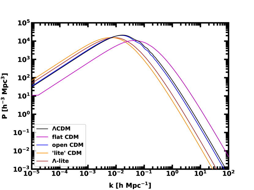
Figure 1: Linear matter power spectra of the models in table 1 normalized to the present epoch with the parameter $\sigma_{8}$. The Fourier transform of the tophat window function that defines $\sigma_{8}$ (light gray curve) highlights its sensitivity to the power in fluctuation modes. The $\Lambda$CDM and open CDM models are nearly identical, demonstrating the strong dependence of $P(k)$ on $\Omega_{\text{M}}$ as compared to $\Omega_{\Lambda}$ or $\Omega_{\text{K}}$.

We next consider the dynamics of matter within voids in these illustrative models to assess the dependence of void dynamics on the background cosmological parameters. We then explore the inverse problem of inferring $\Omega_{\text{M}}$, $\Omega_{\Lambda}$ and $h$ from void properties.

3 Idealized voids

An informative starting point for exploring the connection between voids and their background cosmology is an idealized spherical region with a constant density that is, at some early time, slightly less than the average density elsewhere in the universe. In isolation, this idealized void evolves as if were its own miniature universe with a relatively small matter density and large Hubble parameter [71, 10]. To consider arbitrary density profiles in a range of background cosmologies, we use a numerical approach where we divide spherical voids into thin shells tracked individually from a set of starting conditions [18]. The numerical solutions provide an accurate accounting of the density even as the outer shells cross into the background universe. Appendix A provides the details of the method.

Figure 2 illustrates the evolution of idealized voids in the shell model (cf. [18]). For this exaggerated example, the void is unusually large ($\gg 100$ Mpc) and quite deep, with evolved densities that are much less than the mean of the background universe.

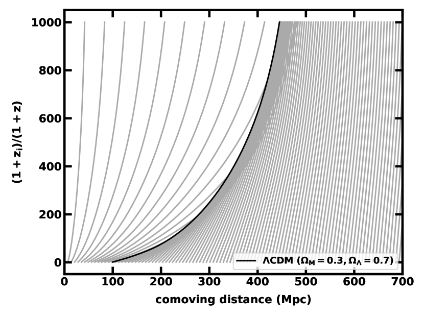
Figure 2: Mass flow lines in a uniform low-density region as a function of the scale factor $a$ for a $\Lambda$CDM cosmological model with starting conditions similar to Ref. [18]. The density inside the region is 10% less than that of the surrounding material at $z=1000$ and all mass elements initially follow the Hubble flow. Each gray line tracks the path of a thin spherical shell. The shells inside the low-density region expand more rapidly than those outside and quickly overtake them. The black curve shows the boundary between the emerging void and the background model where a high-density zone builds and persists.

For a spherically symmetric idealized void, the “shell-crossing radius” — the radius of the innermost shell that has crossed with another larger shell — is a natural definition of the void radius (e.g., the dark solid curve in the left figure 2; prior to shell-crossing, we simply use the radius of the expanding underdense region in the shell simulations). We track the evolution of void sizes for models that start from the same initial conditions (initial redshift and density contrast profile) but with differing background cosmologies. Figure 3 shows the results for the models in table 1. The figure also shows the peculiar velocity — the radial speed in excess of the background expansion directed away from the void center — in units of the local expansion speed within the void.

The curves in figure 3 highlight the following trends:

• Voids grow more robustly with higher cosmic mass density; the void in the flat CDM case ($\Omega_{\text{M}}=1$) grows to the largest size while the void in lite CDM ($\Omega_{\text{M}}=0.1$) is the smallest.

• $\Lambda$ augments the void size at the present epoch when other parameters are fixed. The void in the Lambda-lite model ($\Omega_{\text{M}}=0.1$, $\Omega_{\Lambda}=0.9$) is larger than the one embedded in the lite-CDM model ($\Omega_{\text{M}}=0.1$, $\Omega_{\Lambda}=0.0$).

• Void growth relative to the comoving background generally slows with time and eventually stalls altogether. In high-$\Omega_{\Lambda}$ models, this “freeze-out” occurs quickly as the accelerating expansion overtakes the outflow of matter within voids. In high $\Omega_{\text{M}}$ models, the freeze-out takes a long time.

These trends highlight the relative roles of matter density and dark energy in void dynamics. It is well-known that voids grow to smaller sizes and shallower density contrast in low-$\Omega_{\text{M}}$ models. The open CDM model, once a contender to explain the observed large-scale structure, fails. The addition of dark energy enhances the growth of voids. As mass shells within a void move outward, they jump into a comoving frame that is expanding faster than without dark energy. This effect increases the proper distance between shells and dilutes their mutual gravity thus driving more rapid expansion. Eventually the background catches up.

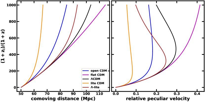
Figure 3: Void sizes and relative peculiar velocities for constant-density spherical voids expanding into a uniform background with the mean cosmic density. The void edges in the left panel correspond to simulations that start off at identical redshift ($z=1000$) and relative depth ($\varepsilon_{\text{init}}=0.01$), but the background universes differ as indicated in the legend. The right panel shows the peculiar velocity — the radial speed in excess of the Hubble flow — relative to the local background expansion speed within the void. The velocities here refer to a shell that starts at half of the initial radius of the underdense region.

Figure 4 gives another view of the impact of both the mass density and dark energy in terms of void depth $\varepsilon$ ranging from 0 (no void) to 1 (vacuum). The models shown in curves run from $\Omega_{\text{M}}=0$ to $\Omega_{\text{M}}=1$, both with and without a cosmological constant ($\Omega_{\Lambda}=1-\Omega_{\text{M}}$ and $\Omega_{\Lambda}=0$, respectively). In contrast with earlier plots, this figure tracks voids with sizes and depths comparable to those observed in the cosmic web.

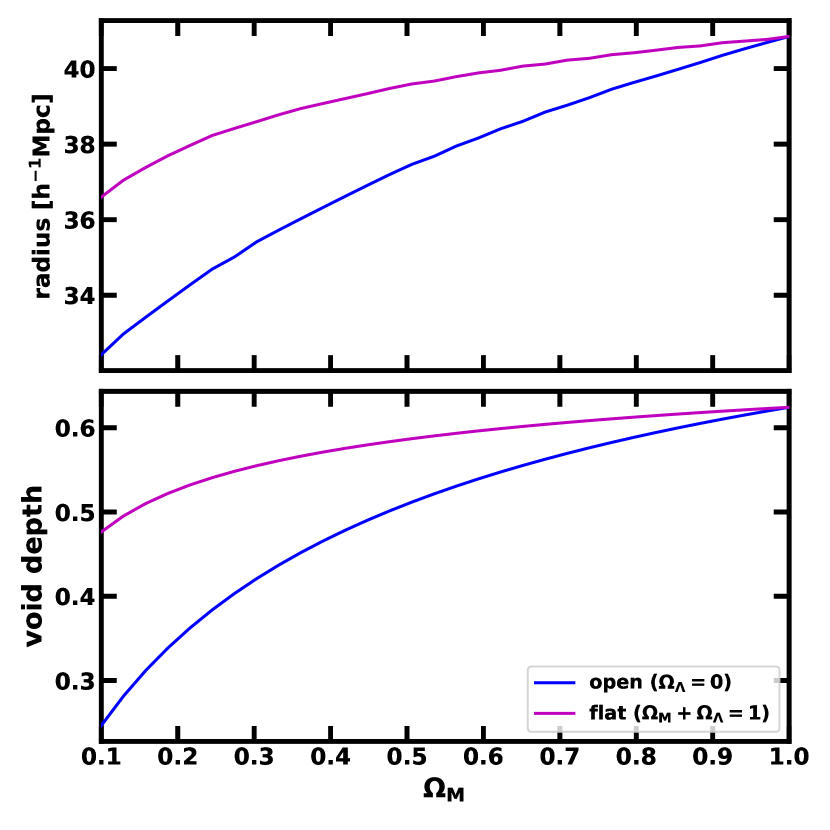
Figure 4: Present epoch void radii and depth as a function of $\Omega_{\text{M}}$ in two sequences of cosmological models. Both the void radii and depth are roughly consistent with the observed power spectrum for initial void sizes of 30 $h^{-1}$Mpc (comoving). Blue curves show open CDM models; magenta curves show geometrically flat models ($\Omega_{\text{M}}+\Omega_{\Lambda}=1$). The void radius increases with increasing $\Omega_{\text{M}}$. At fixed $\Omega_{\text{M}}$, models with a positive cosmological constant produce larger voids than for $\Omega_{\Lambda}=0$.

We next examine the dependence of the depth of voids and the outflow within voids on the cosmological parameters. Figure 4 suggests that a combination of void radius (related to void depth by conservation of mass) and peculiar velocities may contain fingerprints of the background cosmology. To quantify this idea, we explore void growth using linear perturbation theory for large-scale structure formation.

3.1 Linear theory

The shell model provides a route for assessing the full nonlinear evolution of the mass density. However, because voids are relative density fluctuations (equation (2.10)) with amplitudes less than unity, we use linear perturbation theory [67]. The void depth parameter $\varepsilon$ is

$$\varepsilon(r)=\frac{1-\left<\rho\right>_{r}}{\bar{\rho}},$$ (3.1)

where $\left<\rho\right>_{r}$ is the average mass density within a radius $r$ and $\bar{\rho}$ is the mean cosmic density; within a tophat underdensity, $\varepsilon$ is constant. In linear perturbation theory, the depth varies with redshift as

$$\varepsilon_{\text{lin}}(z)=\frac{D(z)}{D(z_{\text{init}})}\varepsilon(z_{\text{init}})$$ (3.2)

where redshift $z_{\text{init}}$ is some initial (or reference) redshift where the depth is known.

Linear theory also predicts flow rates for matter within a void. An effective Hubble parameter, ${H_{\text{eff}}}$, describes the expansion of matter within an idealize void, at least within the shell-crossing radius. For $\varepsilon\ll 1$, linear theory gives

$${H_{\text{eff}}} = \frac{v}{r}=\frac{\dot{a}}{a}+\frac{2a^{3}H}{3\Omega_{\text{M}}H_{0}^{2}r}fg$$ (3.3)

$$= H+\frac{8\pi a^{3}fGH\bar{\rho}\varepsilon}{9\Omega_{\text{M}}H_{0}^{2}}$$ (3.4)

where $r$ and $v=\dot{r}$ are the proper radial distance and radial velocity of matter within the void, relative to the void center. The velocity growth factor $f$ is

$$f\equiv\frac{\dot{D}}{H}$$ (3.5)

where $D$ is the density growth factor in equation (2.12). With

$$\Omega_{\text{M}}H_{0}^{2}=\frac{8\pi G}{3}\bar{\rho}a^{3},$$ (3.6)

the effective Hubble parameter inside the void in units of the background Hubble expansion rate is [72]

$$\frac{{H_{\text{eff}}}}{H}=1+\frac{f\varepsilon}{3}.$$ (3.7)

Because linear theory is limited to small relative density fluctuations, we tune the relationships in equations (3.2) and (3.3) to track the nonlinear solutions from the shell simulations:

$$\varepsilon=\varepsilon_{\text{lin}}\left[1-0.60\varepsilon_{\text{lin}}\left((1-0.27\varepsilon_{\text{lin}}\right)\right],$$ (3.8)

and

$$\frac{{H_{\text{eff}}}}{H}=1+\frac{f\varepsilon\left(1+0.22\varepsilon\right)}{3},$$ (3.9)

for the relative expansion rate inside a void. These relationships hold to within a few percent for voids with depths less that $\varepsilon\approx 0.5$, corresponding to the deepest voids with radii $\gtrsim 25$ $h^{-1}$Mpc in the cosmological models we consider. Coupled with accurate approximations to the growth parameters [73],

$$D\approx\frac{{\Omega_{\text{M}}(z)}}{(1+z)\Omega_{\text{M}}}\ \cdot\ \frac{\Omega_{\text{M}}^{4/7}-\Omega_{\Lambda}+(1+\Omega_{\text{M}}/2)(1+\Omega_{\Lambda}/70)}{{\Omega_{\text{M}}(z)}^{4/7}-{\Omega_{\Lambda}(z)}+[1+{\Omega_{\text{M}}(z)}/2][1+{\Omega_{\Lambda}(z)}/70]},$$ (3.10)

$$f\approx\left[\frac{(1+z)^{3}\Omega_{\text{M}}H_{0}^{2}}{H(z)^{2}}\right]^{0.6},$$ (3.11)

these functions lead to computationally fast predictions of void properties from cosmological parameters. This feature is important to enable the dense sampling required by model parameter fits. Figure 5 provides an illustration.

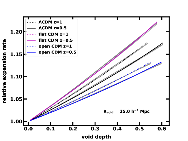
Figure 5: The relative expansion rate inside a void versus void depth for several cosmological models and at two redshifts. The legend lists the shell simulations; the gray curves show the analytic approximations from equation (3.9) for the relative expansion rate (the Hubble parameter inside a void in units of the background Hubble parameter).

The deviation of the void depth $\varepsilon$ from linear theory enables a more accurate estimate of the void radius. According to linear theory, relative to its initial radius at redshift $z_{\text{init}}$, a void deepens but does not grow. From Equation (3.8), nonlinear contributions make the void depth shallower. If this reduction in void depth results from its radial expansion, conservation of mass suggests that

$$\frac{R_{\text{co}}}{R_{\text{co}}(z_{\text{init}})}\approx\left(\frac{\varepsilon_{\text{lin}}}{\varepsilon}\right)^{1/3}$$ (3.12)

Our numerical experiments confirm this trend, although the predicted void sizes are $O(10)$ % smaller than in numerical calculations. One reason for the small difference is that the details of shell crossings, not accounted for in the approximate equation, ultimately determine the void size.

3.2 The Zel’dovich approximation

A related analytical approach for tracking void growth is the Zel’dovich approximation [60, 74, 61] which connects linear and nonlinear phases of structure formation. The Zel’dovich approximation quantifies the displacement of a point particle at some initial position by the peculiar gravity of density fluctuations in the approximation that these fluctuations grow according to linear perturbation theory. For example, a particle sitting at some location in the primordial density field feels some acceleration from the gravity of fluctuations around it. Its subsequent motion is in the direction of that acceleration. At early times when linear theory applies, only the magnitude of the acceleration changes. Thus the motion of the particle is simply along a single displacement vector. This description captures the essence of the Zel’dovich approximation. The approximation is formally dependent on linear theory, but in a Lagrangian or ballistic framework that empowers it beyond linear theory [61].

The Zel’dovich approximation gives the displaced position $\vec{x}$ of a particle that is initially at rest at comoving location $\vec{q}$:

$$\vec{x}=\vec{q}+\vec{\psi}$$ (3.13)

where the displacement vector $\vec{\psi}$ is

$$\vec{\psi}(\vec{x})\sim\vec{\nabla}\phi;$$ (3.14)

here, $\phi$ is the peculiar gravitational potential, related to the density contrast $\delta(\vec{x}$ (equation (2.10)) through the Poisson equation. In the Fourier domain, this expression is simpler [61]:

$$\vec{\psi}=\frac{1}{(2\pi)^{3}}\int d^{3}k\frac{i\vec{k}}{k^{2}}\delta(\vec{k})\exp^{i\vec{q}\cdot\vec{k}},$$ (3.15)

where $\delta(\vec{k})$ refers to Fourier modes of the density contrast. In the approximation, these modes grow at the same rate (equation (2.12)), and the scaling of their collective amplitudes determines the time when the displacement is evaluated. For example, when $\delta$ is scaled to the present epoch, as for the primordial power spectrum in figure 1, $\vec{x}$ gives the location of the particle at the present epoch.

In the Zel’dovich approximation, the particle’s peculiar velocity follows from the time derivative of the displacement:

$$\dot{\vec{x}}=Hf\vec{\psi}$$ (3.16)

where $H$ is the Hubble parameter and $f$ is the velocity growth factor from linear theory (equation (3.5)).

The Zel’dovich approximation is commonly applied in $n$-body codes where particles are placed on a regular grid and density fluctuations are chosen at random based on some primordial power spectrum. The approximation provides displacements and velocities up to a redshift where linear theory applies, and even beyond, so long as particle trajectories do not cross. Because the computational complexity of the Zel’dovich approximation is set by a 3-D Fourier transform, the early stages of evolution in an $n$-body simulation are evaluated rapidly in a single step, without the more intensive calculations of an ordinary differential equation (ODE) solver. The ODE solver takes over only after linear theory breaks down.

Because of its extraordinary effectiveness beyond the linear regime, the “quasilinear” Zel’dovich approximation works well for voids [75], a conclusion that has been compellingly validated for voids as small as 10 $h^{-1}$Mpc with numerical simulation, e.g., [42]. We build on these results. Applying the approximation to spherically symmetric voids, we qualitatively confirm the effectiveness of this approach. Figure 6 shows results for a smooth, compensated void with a depth profile of

$$\epsilon(r)=\left(1-\frac{2r^{2}}{3r_{v}}\right)\exp^{-r^{2}/r_{v}^{2}}.$$ (3.17)

We include results from a full 3-D point-particle code for the Zel’dovich approximation. We introduce the approximation here to demonstrate that it describes void dynamics even when linear perturbation theory breaks down. We rely on this result in section 5.2, below.

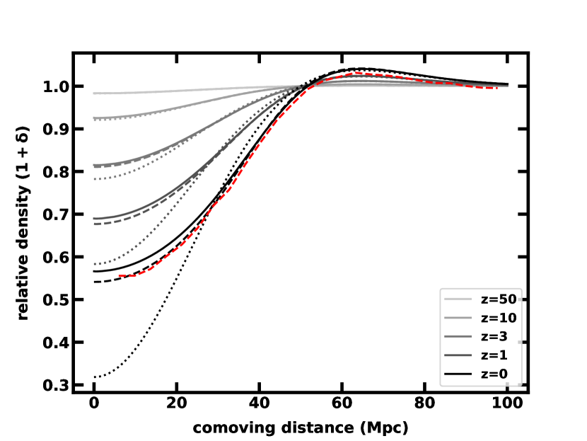
Figure 6: Relative density in a Gaussian-compensated spherical void. The solid curves show the relative density profiles ($\rho(r)/\overline{\rho}$) from direct integration at various redshifts. We include the linear theory predictions (dotted lines) and predictions from the Zel’dovich approximation in 1D (black dashed lines) for comparison. The Zel’dovich approximation from a 3D simulation (red dashed line) provides a trace that has modest “shot noise” from our use of a grid of points. Otherwise it tracks the detailed calculation well.

3.3 The largest voids

Figure 6 demonstrates that linear perturbation theory has limitations even at modest void depth, $\varepsilon\gtrsim 0.2$. The cosmological models have power in density fluctuations that decreases with increasing length scale. At some large scale, $\lambda_{\text{lin}}$, the anticipated void depths are small enough that linear theory applies. We next estimate that length scale.

To determine the linearity scale $\lambda_{\text{lin}}$, we measure the statistic $\sigma_{R}$, the typical relative density fluctuation amplitude in a tophat window function given the power spectrum of a cosmological model. The models we consider are normalized so that the linearity scale is somewhat larger than 8 $h^{-1}$Mpc; for “1-$\sigma$” fluctuations in a $\Lambda$CDM universe, $\sigma_{R}$ dips below 0.2 at a length of just under 40 $h^{-1}$Mpc. However, voids this large may arise from more rare, deeper fluctuations. In a volume of radius $R_{\text{3G}}\equiv 3,000$ $h^{-1}$Mpc, there are approximately $R_{\text{3G}}^{3}/4R^{3}\sim 10^{4}$ non-overlapping samples of the density field convolved with a tophat of radius $R=40$ $h^{-1}$Mpc. Assuming Gaussian statistics and statistical independence of samples, we expect a “one-of-a-kind” fluctuation of $3.7\times 0.2$, or, equivalently, a void depth of over 0.7, well beyond the reach of linear theory (figure 6). Thus $\lambda_{\text{lin}}$ must be considerably larger.

Figure 7 provides a comparison of void depths from 1-$\sigma$ fluctuations, one-of-a-kind void depth from linear theory, and the one-of-a-kind depth when evolved with the shell simulator. As in figure 6, linear theory apparently breaks down at a void depth $>0.2$. For the $\Lambda$CDM normalization we adopt, a good choice for $\lambda_{\text{lin}}$ is $\sim 90~{}{\rm Mp}$c. This length is similar in the open CDM model and smaller, about 70 $h^{-1}$Mpc, in the other models we explore as a result of the choice of (low) power normalization at translinear length scales.

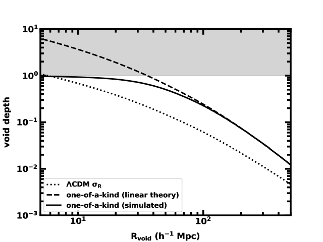
Figure 7: Void depth as a function of void radius for spherical tophat underdensities in the $\Lambda$CDM model. The $\sigma_{R}$ curve (dotted line) shows the linear theory prediction of void depth for a 1-$\sigma$ fluctuation. The “one-of-a-kind” curves are the prediction of void depth for fluctuation amplitudes that are rare. We expect only one such void in a survey volume with radius 3,000 $h^{-1}$Mpc. Linear theory noticeably deviates from the shell simulation results when the void depth exceeds 0.2. The breakdown occurs at a window radius around 90 $h^{-1}$Mpc.

This analysis suggests that a search for the largest voids in the universe should rely on linear theory only for scales larger than $\sim$90 $h^{-1}$Mpc. At smaller scales, the predictions of direct simulations provide more robust comparisons between theory and observations.

3.4 Cues from idealized voids

Shell simulations of idealized cosmic voids (Appendix A) provide a testing ground for understanding voids and their connection to the background cosmology. The main results are:

• The evolution of void size, depth and radial outflow reflect the background cosmology. The detailed evolution of these properties is well approximated by linear theory for shallow voids (depth $\varepsilon\equiv 1-\delta\lesssim 0.2$); the Zel’dovich approximation gives more accurate results for deeper voids.

• The depth of the largest voids, related directly to the power spectrum of fluctuations, is well approximated by linear perturbation theory only for scales above a threshold, $\lambda_{\text{lin}}$, around 70–80 $h^{-1}$Mpc.

• Void depth and outflow rate are simply connected by an analytical expression, equation (3.9), a modest extension to linear theory. This expression allows estimates of $fH$ (the velocity growth parameter times the Hubble parameter of the background universe) as a function of redshift independent of void radius.

The analytical expression in equation (3.9) is a central result. In principle, with samples of $fH$ over a range of redshifts, we can estimate cosmological parameters in a manner similar to studies of Type 1a supernova [76]. We next amplify this result.

4 Cosmological parameter estimation from idealized voids

The interior regions of idealized voids evolve as isolated mini-universes. They have FLRW parameters of their own. Nonetheless there are two key connections between voids and the background cosmology. The first connection is the void depth $\varepsilon$, which relates the matter density inside a void to the mean density of the universe. The second connection is equation (3.9), which links $\varepsilon$ and the outlow rate ${H_{\text{eff}}}$ to $fH$, where $f$ is the velocity growth parameter (equation (3.5)) and $H$ is the background Hubble parameter. Just as samples of $H(z)$ from Type Ia supernovae yield $\Omega_{\text{M}}$, $\Omega_{\Lambda}$ and $h$, samples of $fH$ from void properties $\varepsilon$ and ${H_{\text{eff}}}$ can provide cosmological constraints. Any set of voids can, in principle, provide constraints, so long as their statistical properties are recovered at a range of redshifts.

4.1 Maximum likelihood and MCMC

To demonstrate that simple void properties lead to estimates of cosmological parameters, we run nonlinear shell simulations $n_{v}$ times. We vary the starting conditions and stopping times to obtain a single measurement of $\varepsilon$ and ${H_{\text{eff}}}$ for each of $n_{v}$ unique voids. The stopping times sample redshifts ranging from $z=0$ to $z=2$. To fit the simulated values of ${H_{\text{eff}}}$ with cosmological model predictions, we define a goodness-of-fit measure

$$\chi^{2}=\sum_{i=1}^{n_{v}}\left[y_{i}^{\text{(measured)}}-y_{i}^{\text{(theory)}}\right]^{2}/\sigma_{i}^{2}$$ (4.1)

where $y_{i}^{\text{(measured)}}$ are samples of the simulated outflow rate scaled by a factor of

$${H_{\text{ref}}}=100(1+z)^{3/2}~{}\text{km/s/Mpc},$$ (4.2)

to keep numerical values close to unity. The theoretical values, $y_{i}^{\text{(theory)}}$  come from using the measured depths $\varepsilon_{i}$ in equation (3.9) with a given set of parameters $\Omega_{\text{M}}$, $\Omega_{\Lambda}$ and $h$. The “uncertainties” $\sigma_{i}$ in the expression for $\chi^{2}$ are

$$\sigma_{i}^{2}=\sigma_{y,i}^{2}+\frac{f^{2}\eta^{2}}{9}\sigma_{\varepsilon,i}^{2},$$ (4.3)

where the $\sigma_{y}$ and $\sigma_{\varepsilon}$ correspond to noise levels in outflow and depth respectively. The quantities $f$ and $\eta={H_{\text{eff}}}/{H_{\text{ref}}}$ are determined for a given model at the redshift of the $i^{\text{th}}$ void. The noise model adopted here is that measurements have normally distributed fractional errors at a level $e_{\text{rel}}\sim 0.001$–0.1. By including the noise at some tunable level, we can identify correlations in fitted parameters and assess the impact of observational errors.

We use a maximum-likelihood approach to fit measurements with model parameters. In this framework, a likelihood function $\cal{P}$ returns the probability of obtaining specific measurements ($\varepsilon$, ${H_{\text{eff}}}$) given a set of model parameters ($\Omega_{\text{M}}$, $\Omega_{\Lambda}$, $h$). Fitting measurements with models amounts to sampling and maximizing $\cal{P}$ in parameter space. We use the emcee Markov-chain Monte Carlo (MCMC) package [77] to do the sampling, with multiple “walkers” mapping out the probability distribution $\cal{P}$ in the domain $\Omega_{\text{M}}=[0.045,1]$, $\Omega_{\Lambda}=[0,1]$, $h=[0.5,0.9]$. We use uninformative priors (all models in this domain are equally likely). We thus distribute the starting location of the walkers in parameter space with a low-discrepancy quasirandom number generator (scipy.qmc). We determine best-fits from the global maximum of the likelihood function as mapped by the MCMC walkers; we obtain uncertainties and correlations between parameters from the distribution of samples in parameter space.

Output from the MCMC sampling highlights the cosmological information contained in voids. The panels showing corner plots in Figure 8 illustrate likelihood samples from one, two and three voids, each at a unique redshift. All of the depths and outflows have small ($e_{\text{rel}}=0.1$%) uncertainties. With a single void at $z=0$ and one data point $(\varepsilon_{1},y_{1})$ (upper panel), the likelihood distribution for $h$ is the narrowest compared with the search domain. The void thus contains the most information about the Hubble parameter. The fit is significantly less sensitive to the matter density parameter $\Omega_{\text{M}}$. However, $\Omega_{\text{M}}$ and $h$ are strongly anticorrelated. Thus if $h$ is known a priori, $\Omega_{\text{M}}$ may be more accurately determined. The likelihood distribution for $\Omega_{\Lambda}$ is flat and there is no apparent correlations with other parameters. We conclude that a single void, a snapshot in cosmic time, offers little information about cosmic acceleration.

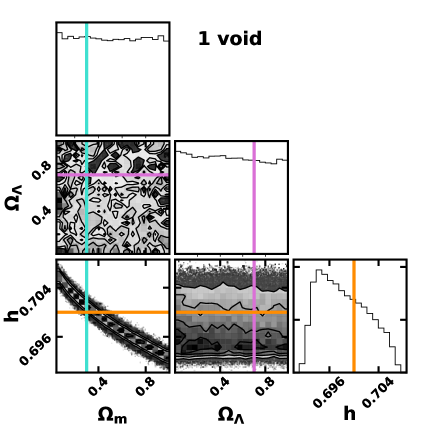
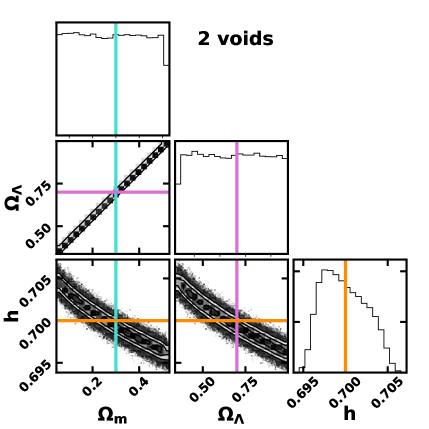
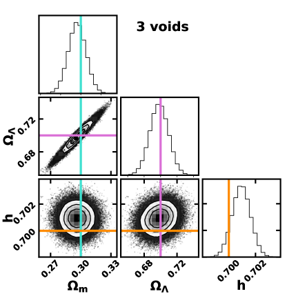
Figure 8: A corner of corner plots [78] showing probability distributions for parameter fits to void depth and outflow rates. The labels indicate the number of voids measured. The lines locate the true values of the parameters $h$ (orange), $\Omega_{\text{M}}$ (turquoise), and $\Omega_{\Lambda}$ (blue). The fits are most sensitive to $h$, then $\Omega_{\text{M}}$, and finally $\Omega_{\Lambda}$. In the upper corner plot, showing likelihood distributions for a single void, only the Hubble parameter is well constrained. Asserting prior knowledge of $h$ at its true value selects the probability distribution in a slice along the orange lines. With that prior, the (posterior) probability distribution for $\Omega_{\text{M}}$ becomes sharply peaked around its true value. In the lower left corner plot (two voids, $z=0$ and $z=1$), both $h$ and $\Omega_{\text{M}}$ are well constrained. In the lower right panel, with three voids ($z=0,0.5,1$), $\Omega_{\Lambda}$ is also well constrained.

The likelihood distributions for measurements of two and three voids (figure 8) further emphasize that voids measured at three or more distinct redshifts are necessary to constrain the cosmological parameters. Two voids provide weak constraints on $\Omega_{\Lambda}$, but only with prior knowledge of either $h$ or $\Omega_{\text{M}}$.

4.2 The redshift range

The Hubble diagram built from Type Ia supernovae provides better constraints on cosmological parameters when applied over a large redshift range [79, 80]. In analogy voids provide better constraints when we measure $fH$ as a function of $z$. Figure 9 illustrates this effect based on samples of 100 voids spaced uniformly in $z$. The broadest range of redshifts ($z=0$–2) yields the tightest constraints..

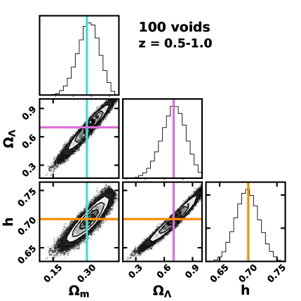
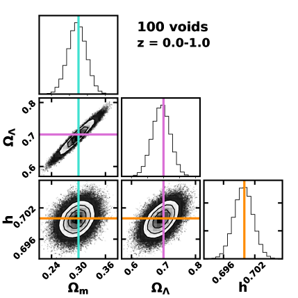
Figure 9: Corner of corner plots with probability distributions of cosmological parameters from samples of voids covering different redshift ranges. Each sample includes 100 voids from shell simulations with noise at the 1% level. From the narrowest redshift range (upper left) to the broadest (lower right), the constraints improve significantly.

There are two main challenges for measuring voids properties over a wide redshift range. At low redshift, the observable volume available to sample voids is small — in an absurd limit, there can be at most only one void of radius 100 $h^{-1}$Mpc within a survey of that depth. At high redshift the challenge is measurement of void properties from faint and distant galaxies. For this theoretical demonstration of the connection between void parameters and the underlying cosmology, we consider only the first challenge, identifying the number of voids we expect as a function of redshift.

Figure 10 shows the number of voids in redshift bins from $z=0$ to $z=2$ with $\Delta z=0.1$ in a $\Lambda$CDM universe. At the lowest redshift, with $z\leq 0.1$, the survey volume is a sphere of radius of about 300 $h^{-1}$Mpc. As in the figure, we find 50 voids in that region. This number count matches our expectation for 30 $h^{-1}$Mpc voids that represent the least dense quartile of independent samples of the matter density field smoothed at scale $R$. We assume that this tail of the void depth distribution represents detectable voids, even at $z>0$, and that the comoving space density of voids remains constant for the redshifts we consider. If we count only voids deeper than a certain threshold independent of redshift $z$ then we lose some voids at $z>0$ because they are less evolved. As we move outward to bins at higher redshift, the geometric increase in the volume sampled grows rapidly. At $z=0.3$ and above we anticipate a thousand voids or more. The dependence of comoving distance on redshift limits the number of anticipated voids to less than $10^{4}$ per bin at higher redshift. At a redshift of $\sim$2.5, the proper volume per bin as well as the number of voids begins to fall with increasing redshift. If we set a depth threshold independent of redshift, then we lose some voids at redshift $z>0$ because they are less evolved. We estimate with a threshold of $\sim$0.2, we still retain over a thousand $\sim$30 $h^{-1}$Mpc per bin for $0.4\lesssim z\lesssim 2$. The bins with the most voids (over 2,000) are at redshifts of $z\approx 1$.

Figure 10: The number of voids in a $\Lambda$CDM universe in redshift bins of width $\Delta z=0.1$. For this estimate, we use the top 25% deepest underdense regions in the primordial density field smoothed on a scale of 30 $h^{-1}$Mpc. These regions evolve into present-day voids with a depth of 0.2. The red-colored histogram gives the number of these regions in each redshift bin. The blue-colored histogram shows the subset of these voids that have reached that 0.2 depth at the median redshift of their bin.

4.3 Summary of cosmology from idealized voids

By measuring void depth $\varepsilon$ and outflow rate ${H_{\text{eff}}}$ in voids at multiple redshifts, we build samples of $fH$ that provide constraints on $h$, $\Omega_{\text{M}}$ and $\Omega_{\Lambda}$. This procedure mimics the approach to cosmological constraints based on Type Ia supernovae [76]. Preliminary tests with fits to shell simulation measurements indeed suggest that samples of void properties over a range of redshifts provide robust cosmological parameter estimates. Fits based on the analytical approximation in equation (3.3) (section 3.1) are fast and effective.

5 Voids in numerical realizations of the cosmic web

We run an $n$-body code to simulate large chunks of the universe and to evaluate the cosmological information encoded by voids. Our approach is based on the adhesion approximation [64]; similar $n$-body realization methods include the PATCHY code [81]. We use the Zel’dovich approximation in step-wise fashion; we allow particles to free stream with updates as large-scale structures emerge. Critically, the adhesion approximation adds small-scale viscous diffusion to mitigate the problem of trajectory crossings that arise when free streams of matter in the Zel’dovich flows pass right through one another. Appendix B summarizes the implementation.

We adopt the adhesion approximation primarily because it is a fast, accurate way to track void dynamics. Because density fluctuations within voids are low amplitude, nonlinear dynamical effects are weak. Recent work [39, 63, 42] demonstrates that voids are well suited to the Zel’dovich approximation and the related adhesion algorithm. The realizations of large-scale structure we construct are geared toward the void-dominated linear regime; they are distinct from full $n$-body simulations that track small-scale nonlinear dynamics with Poisson solvers and ODE integrators.

We generate realizations of the cosmic web in various cosmological models (table 1) with $n=256^{3}$ to 2048³ point particles in cubic regions of 250 to 5000 $h^{-1}$Mpc to a side. Each realization provides a statistically independent snap shot of positions and velocities of mass tracers at a user-specified redshift. In one mode we also construct lightcones where redshift is a function of distance from the center of the realization as in a mock redshift survey. Figure 11 shows an example.

Figure 11: Realization of large-scale structure in a lightcone that extends beyond a redshift of $z=1$. The color indicates the local mass density in an $x$-$y$ plane, where positions $x$ and $y$ are comoving coordinates with an observer located at the origin. The origin indicates a point in space at the present epoch. Density structures near the origin are evolved to the present time. Moving away from the origin corresponds to moving back in time, or equivalently, increasing redshift, when structures are less evolved. The circles about the origin show the location of points at redshifts 0.1, 0.5 and 1, as labelled. By a redshift of $z=1$, the density fluctuations are noticeably weaker than at the origin. The inset is a zoomed-in view of a region within a redshift of $z=0.1$ (indicated by the circle).

5.1 Finding voids

A key step in assessing the connection between voids and their background cosmology is finding the voids. This process is complex mainly because the cosmic web is not Swiss cheese or even spongelike, with nicely spherical holes embedded in a high-density background. Instead, choices about density thresholds (voids are not vacuums), sizes and shapes are necessary and lead to a plethora of distinct void-finding algorithms, e.g., [17, 19, 31, 82, 83, 84, 40, 85, 86, 87].

We identify voids in the $n$-body realizations that resemble the spherical shell models in section 3 in a straightforward way. Our algorithm specifically targets voids with user-selected radii between $R_{\text{min}}$ and $R_{\text{max}}$:

1. Interpolate point particles to estimate the local mass density at points on a regular 3D grid in comoving coordinates of size $L$ per side. With the $n$-body realizations, we use a linear (“cloud-in-cell”) interpolation scheme that respects the periodic boundary conditions of the realizations.

2. Smooth the density grid on a scale $R_{\text{smoo}}$ between $R_{\text{min}}$ and $R_{\text{max}}$. For the $n$-body realizations, we use FFT-based convolutions with a 3D tophat window function of radius $R_{\text{smoo}}$.

3. Identify isolated local minima in the smoothed density field; each one has a value less than the mean and is the most extreme in a spherical volume of radius $2R_{\text{smoo}}$ centered on it. We use the function minimum_filter in the scipy.ndimage module for this process. These minima are void candidates.

4. Apply a mean depth threshold. To focus on voids of unusual depth, we ignore void candidates with minima less than two times $\sigma_{R}$, where $R=R_{\text{smoo}}$.

5. Estimate the radius and depth of each void candidate. This process begins with an estimate of the central void depth, the average depth within $R_{\text{smoo}}/2$ of the location of each isolated minimum. Then we build a smoothed radial density profile by binning particles in concentric shells about the minimum or by averaging adjacent sets of radially-sorted grid values. The void radius, $R_{\text{void}}$, is the distance from the void center where the void profile is half of the central void depth.

6. Accept a void candidate if its radius is between $R_{\text{min}}\leq R_{\text{smoo}}$ and $R_{\text{max}}$. Otherwise reject the candidate.

Figures 12 and 13 illustrate the results. Figure 12 shows a slice through an $n$-body realization and a few of the voids that intersect the slice. Figure 13 provides radial density profiles of voids calculated from the mass density averaged in concentric spherical shells. Although there is considerable variation from profile to profile, the average radial density profile is characterized by a flat well with a moderately steep rise near the void edge.

Figure 12: Example of the void finder ($R_{\text{smoo}}=30$ $h^{-1}$Mpc) in a $\Lambda$CDM realization ($L=500$ $h^{-1}$Mpc, $n=512^{3}$). The circles mark voids located within a smoothing length of the slice shown. The realization is shifted to put the deepest void at the origin.

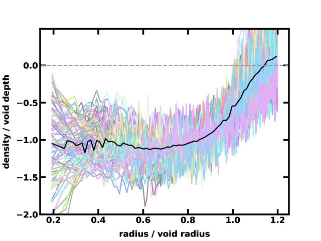
Figure 13: Radial density profiles of voids from the lightcone realization in figure 11. Void radii range from 50 $h^{-1}$Mpc to almost 300 $h^{-1}$Mpc. Although individual void density profiles (the slurry of light colored lines) vary, on average (black curve) the profiles are similar to tophat window functions with a smoothed step.

To explore the properties of void depth and outflow rate as in section 3, we select $n$-body particles within each void and measure their number density averaged within a radius $R=R_{\text{void}}/2$. This value is the basis for the depth $\varepsilon$ assignment. The outflow comes from averaging radial velocities of particles relative to the void center in some spherical shell with thickness $0.1r$. The average $v_{r}$ divided by $r$ estimates the outflow rate ${H_{\text{eff}}}$.

The void-finding algorithm we use is straightforward and fast. It identifies underdense regions reminiscent of the simple, spherically symmetric idealized voids of section 5.2 (the void in the center of figure 12 is an example). The algorithm also selects some voids with complex internal structure or non-spherical shapes. These voids differ significantly from idealized voids and produce the “scatter” in figure 13. This approach connects the idealized spherical void approximations to a more realistic simulation of the observed large-scale structure of the universe.

5.2 Cosmological parameter estimation

Following the broad approach of section 4, we measure two characteristic void properties, void depth $\varepsilon$ and outflow rate ${H_{\text{eff}}}$, at the half radius of each void. With a catalog of voids at various redshifts, we build a set of samples of these properties. If the void behavior is analogous to the idealized ones, the sample sets yield estimates of $fH$, where $f$ is the velocity growth factor and $H$ is the redshift dependent Hubble parameter of the background cosmology. Figure 14 illustrates this approach with $\sim 30\pm 5$ $h^{-1}$Mpc voids in a set of six realizations of the cosmic web at redshifts from 0 to 1. Although there is variation from point to point relative to the relationships between ${H_{\text{eff}}}$ and $\varepsilon$ from linear theory, the overall trends are clear.

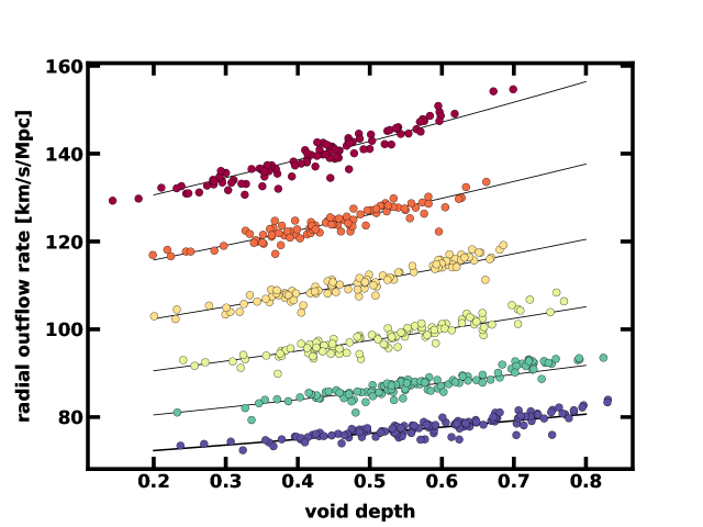
Figure 14: Void depth versus outflow rate for six realizations at various redshifts. The colored points are from $\sim$30 $h^{-1}$Mpc voids identified in $n$-body realizations; the red symbols correspond to redshift $z=1$ and blue for $z=0$. The solid curves are the theoretical predictions from linear theory calibrated with the spherical shell model. The theoretical approximations are tuned for shallower voids ($\varepsilon<0.6$), and their breakdown at higher void depth is evident.

The theoretical curves in figure 14 are fingerprints of the background cosmology. To extract cosmological parameters by fitting the $n$-body samples shown in figure 14 with the fingerprints from various cosmological models, we use the same MCMC-based parameter estimators as in section 4: We seek values in a parameter space of $\Omega_{\text{M}}$, $\Omega_{\Lambda}$ and $h$ using a $\chi$-square measure to assess the goodness of fit between theory (equation (3.9)) and samples of $(\varepsilon,{H_{\text{eff}}})$ from voids in the $n$-body realizations. Our priors are uniform inside the domain $0<\Omega_{\text{M}}<1.05$, and $-0.1<\Omega_{\Lambda}<1$, expanded slightly from the analysis of idealized voids to better explore the sensitivity of the estimators. The scatter in the samples used arises from deviations of the $n$-body realization voids from the ideal ones.

Figure 15 shows results for the $\Lambda$CDM model (table 1). The figure highlights the central result: void depths and outflow rates are effective as cosmological probes. They offer new, independent constraints on the parameters that characterize the background universe. The three panels show different redshift ranges for the samples and illustrate that the approach is most effective with a broader redshift range.

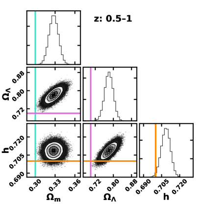
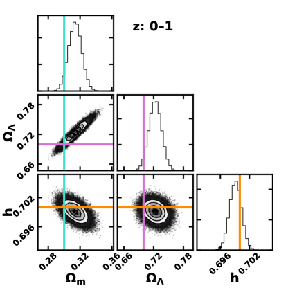
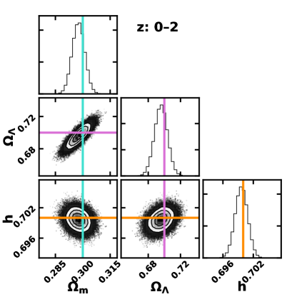
Figure 15: Corner of corners plot [78] showing MCMC samples in parameter space for independent realizations of the $\Lambda$CDM model at redshifts from $z=0$ to $z=2$. Each realization lies in a cube of 500 $h^{-1}$Mpc to a side and has $n=512^{3}$ points. Voids of radii $30\pm 5$ $h^{-1}$Mpc are included. As in figure 9 for the ideal voids, the panels illustrate that a broader range of redshifts among void samples enhances parameter estimation.

5.3 The largest void in the universe

The distribution of void sizes can provide a powerful test of the background cosmology [20]. Here we focus on “the largest void”. The existence of extremely large voids may place strong constraints on the background model parameters [18]. The void identification criteria for this investigation are only slightly more stringent than finding local minima in tophat-smoothed density fields [23]. Voids in our catalog have profiles that are deep in their central region, and rise to a half-depth value at the nominal radius, behavior that requires specific phase alignment between density fluctuation modes. Supervoids — composed of multiple smaller voids — might be missed by our algorithm, depending on their substructure.

The void finder incorporates a depth threshold filter that requires voids to be at least a 2-$\sigma$ fluctuation in a density field smoothed on a scale comparable to the void size. This cut ensures that voids are significantly underdense. This cut and the requirement that density in a void is consistently low throughout the central regions favor voids that more closely resemble the idealized. This aspect is important for applying the formalism of $4. We may miss some reasonable voids that could be identified by other algorithms, but our search for the largest void errs on the side of caution.

Figure 16 shows an example of large voids within the lightcone realization of 5000 $h^{-1}$Mpc to a side. Because of grid effects, density modes are poorly sampled for voids with radii $\gtrsim$250 $h^{-1}$Mpc. All depths are scaled to the present epoch. For comparison, we also show the Eridanus Supervoid parameters [23]. The 1-$\sigma$ errors for the supervoid suggest that it is consistent with voids predicted in the $\Lambda$CDM realization. Since its initial discovery, the supervoid region has been reanalyzed [25, 26]. The supervoid is estimated to have a greater depth and smaller radial extent, but it is still consistent with standard theory.

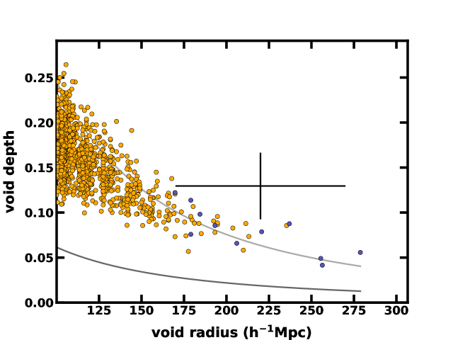
Figure 16: Void depth versus size of the largest voids in a 5000 $h^{-1}$Mpc lightcone realization. This depth-size diagram applies to voids larger than 100 $h^{-1}$Mpc, scaled according to linear theory. The depth is effectively at the present epoch. The darker solid curve is $\sigma_{R}$ from the linear power spectrum; we eliminate void candidates with amplitudes below this value. The lighter-tone line is the amplitude of a one-of-a-kind void predicted in linear theory for the survey volume. The color of each sample point indicates whether the void is a “subvoid” (orange) or a void that is not embedded in a larger void (blue). The error bars show the observed Eridanus supervoid [23].

Figure 17 illustrates radial density profiles of the largest voids. These profiles are in physical/real space, not redshift space.

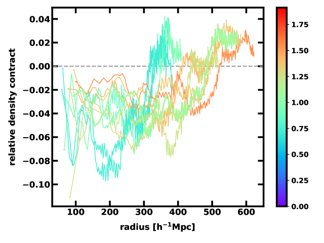
Figure 17: Radial density profiles of the largest voids in a 5000 $h^{-1}$Mpc lightcone. The panel shows the profile of the top ten largest voids.

6 Voids in redshift space

So far, we have used the positions and peculiar velocities of galaxies as tracers to constrain the background cosmological parameters (section 5.2). However, observations do not yet measure accurate distances. Instead, extensive galaxy surveys provide the distribution of objects in redshift space. Here we consider the cosmological information content of voids as mapped in redshift space [88, 41, 62, 50, 89, 51, 52].

An idealized void, with uniform depth $\varepsilon$ and constant outflow ${H_{\text{eff}}}$, contains galaxies that map from real space to redshift space according to

$$\vec{s} \approx \vec{S}+H\vec{r}+\hat{e}_{\text{los}}\cdot\vec{v}\hat{e}_{\text{los}}$$ (6.1)

$$\approx \vec{S}+H\left(\vec{r}+\frac{f\varepsilon\Delta_{\text{los}}}{3}\hat{e}_{\text{los}}\right)$$ (6.2)

where $\vec{S}$ is the redshift-space location of the void center at some distance from the observer, $H$ is the Hubble parameter at that redshift, and $\Delta_{\text{los}}$ is a real-space coordinate along the observer’s line of sight relative to the void origin. We assume that the void is observed at a large distance $R\gg R_{\text{void}}$, so that the unit vector along the line of sight, $\hat{e}_{\text{los}}$, is nearly constant for all points throughout the void.

The transformation from real to redshift space increases the apparent depth of a void [72]. A small region in real space within an idealized void is stretched in redshift space along the line-of-sight by a factor of ${H_{\text{eff}}}/H$. The void thus appears deeper in redshift space:

$$\varepsilon_{s}=\left(1+\frac{f}{3}\right)\varepsilon$$ (6.3)

This enhancement is substantial — about 17% for the $\Lambda$CDM model at $z=0$. The effect is important when assessing the size and depth of voids.

Redshift surveys contain information about velocity flows. Statistics of clustering in redshift space are sensitive to redshift space distortions [72]. For voids, the net fractional elongation along the line-of-sight tends to be small because the outflow velocities are small compared with the Hubble flow across the void diameter. We focus on this overall shape distortion to estimate the outflow.

In the ideal case, we define the shape of voids in redshift space based on the location of particles at the interface with the background universe. Neglecting any shell crossings, we approximate a distant, redshift-space void as a prolate ellipse, with geometric eccentricity

$$e={H_{\text{eff}}}/H-1\approx\frac{f\varepsilon}{3}.$$ (6.4)

This result is fragile. It depends critically on the spherical symmetry of the underlying real-space density field and on the ability of analysis algorithms to identify the void boundary.

Figure 18 shows the real-space and redshift-space densities in the vicinity of an idealized void. The figure offers two lessons: first, the increase in void depth in redshift space from its value in real space is significant. This factor is important in analyses of void properties inferred from redshift space. The second lesson is that the geometric distortion of real-space patterns in redshift space is, as expected, small. The void in figure 18, with a depth in real space of $\varepsilon\approx 0.4$ in a background $\Lambda$CDM cosmology at $z=0$, has an eccentricity of $\sim$0.07.

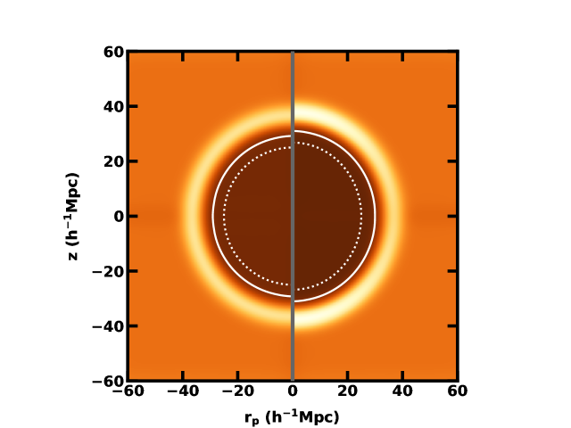
Figure 18: An idealized compensated tophat void in real and redshift space. The real mass density is on the left; the redshift-space counterpart is on the right. The solid line is an isodensity contour at 50% of the central depth. The dashed line shows positions of points on a circle in real space and its elliptic counterpart in redshift space, assuming that the points comove with the expansion of the void. The image has been smoothed with a Gaussian filter (standard deviation of 2 pixels) to remove grid effects.

Successful strategies to tease out the small amplitude distortion of void geometry in redshift space focus on combining data from multiple voids. Aggregate measures like the void-galaxy correlation function quantify averaged redshift-space distortions that emerge away from the void centers, revealing a mean peculiar motion [88]. For idealized voids, this information is equivalent to the mean eccentricity at the void boundary. In general, when calibrated with numerical simulations, void-galaxy correlations are impressively effective as cosmological indicators [50, 89]. Outcomes include a measure of dark energy with the Alcock-Paczynski effect and the velocity growth parameter $f$, e.g., [50, 90, 51, 91].

More information from individual voids mapped in redshift space comes from density and velocity field reconstruction methods [92, 47, 93, 94, 95, 96, 97, 98, 99, 100, 61], including those tuned to redshift-space distortions in the region of voids [88, 62]. These algorithms reverse-engineer the real-space density and peculiar velocity fields from redshift maps. Their application is recommended prior to void identification so that distortions in geometry and void depth do not introduce adverse selection effects, e.g., [101, 65].

The transformation from redshift space to real space requires assumptions about the background cosmology e.g., [72]. The Hubble expansion rate $H$ and velocity growth factor $f$ are typically the only inputs for reconstruction methods, and are the only fitting parameters in the model estimation analysis of section 5.2. Following the lead of [47], preliminary work suggests cosmological constraints from reconstructed voids at various redshifts are possible. We plan to investigate these issues in future work.

7 Conclusion

Cosmic voids hold a bounty of information about the overall content, structure, and evolution of the universe [14, 102, 10, 11, 12, 18, 29, 47, 32, 33]. Because voids contain comparatively little matter, the effects of dark energy on the dynamics of visible objects lead, in principle, to testable model-dependent predictions [103, 32, 104, 105, 34]. The mere presence of the “largest void,” is one test of models [18].

We explore how void dynamics can constrain the parameters of the underlying cosmology. We enhance the approaches of [18] and [42] where simple models and linear theory are applied to voids. We also build numerical infrastructure to simulate idealized voids and to generate $n$-body realizations of voids that emerge in a cosmological context. We focus on voids with sizes larger than 20 $h^{-1}$Mpc. We use simulation volumes that are between 250 $h^{-1}$Mpc and 5000 $h^{-1}$Mpc to a side. At the largest scale, an individual $n$-body realization provides representative samples of voids with radii up to $\sim$250 $h^{-1}$Mpc.

The numerical data here include fifteen $n=512^{3}$ independent $n$-body realizations (figure 15) and one $n=1024^{3}$ lightcone snapshot (figure 11). Other data sets in this project include more than 100 realizations with $n=512^{3}$ and a dozen $n=1024^{3}$ realizations, spanning a range of redshifts, cosmological models (table 1) and random number seeds (Appendix B). The adhesion algorithm is a distinctive feature of this approach because it is at least an order of magnitude faster than full $n$-body simulations [64]. The adhesion approximation offers the possibility of maximum-likelihood fitting to void data with realizations evaluated at unique sets of cosmological parameters instead of the analytical approximation in equation (3.9). Thus, we can include deep voids ($\varepsilon>0.5$) in parameter estimation even when though the analytical approximation breaks down.

The main results are:

• Idealized voids demonstrate the dynamical role of dark matter and dark energy in the simple case of a cosmological constant. The trajectories of matter (galaxies) in idealized voids — the radial position and velocity — are sensitive to both $\Omega_{\text{M}}$ and $\Omega_{\Lambda}$. Each set of parameters produces a unique path in this phase space (figure 3).

• We confirm that linear theory and the Zel’dovich approximation provide good descriptions of the dynamics of ideal voids (figure 6). Linear theory, with slight modifications, connects void depth $\varepsilon$ and outflow rate ${H_{\text{eff}}}$ to the background cosmological parameters $H$, $\Omega_{\text{M}}$, and $\Omega_{\Lambda}$ through dependence on the overall background expansion and the velocity growth parameter $f$.

• When measured over a range of redshifts, void properties $\varepsilon$ and ${H_{\text{eff}}}$ give estimates of the Hubble parameter, $H(z)$, at different cosmological times. As with analyses of Type Ia supernovae, these values in turn reveal the expansion history of the universe as a whole, and thus constrain $\Omega_{\text{M}}$ and $\Omega_{\Lambda}$. We estimate the cosmological parameter using both idealized voids and more realistic samples generated with $n$-body simulations based on the adhesion approximation (figures 8 and 15).

• We generate lightcone maps from $N$-body realizations. These lightcones simulate the large-scale structure observed in redshift surveys. With a simple void finding algorithm, we explore the properties of the largest voids in the simulated observable universe. Observed “supervoids” spanning hundreds of megaparsecs are likely in the $\Lambda$CDM model.

• We focus on void properties in real space including exploration of their physical mass densities and outflows. This demonstration of principle may eventually lead to observational constraints with much improved direct distance measurements.

• Current maps of large-scale structure are primarily redshift surveys. We discuss interpretation of the properties of the largest voids in redshift space (accounting for the Kaiser effect). Voids appear deeper in redshift space than they are in real physical space.

• To forecast future parameter estimation from voids in redshift surveys, we briefly mention adopting real-space reconstruction algorithms that extract physical void depths and outflow rates from redshift survey data [47]. This avenue may eventually be promising at $z\sim 1$ where the number of voids that can be accessed observationally is large.

To explore what we might learn from voids, we study the simulated universe where we have full knowledge of void density profiles and outflow velocities. Simple void properties derived from these quantities constrain parameters of the background cosmology, providing independent tests from low density regions where the dynamical effects of dark energy are enhanced. Current observations can not measure these properties well enough to apply the approach we describe. With improvement of observational capabilities over time, we may eventually realize the full potential of cosmology with voids.

Appendix A The shell model

We track void evolution using thin, concentric shells, each with an assigned mass uniformly distributed within it [18]. Newtonian mechanics provides the framework for tracking the detailed evolution of these shells over distances that are much smaller than the Hubble length, $c/H_{0}\approx 4,000$ Mpc. We consider initial conditions as in [18], with a spherical, constant-density region that is underdense relative to the rest of the universe by some small factor, $\varepsilon_{\text{init}}$. The initial mass density is

$$\rho_{i}=\bar{\rho}\left[1+\delta\right]=\frac{3H_{0}\Omega_{\text{M}}}{8\pi Ga_{i}^{3}}\times\begin{cases}1-\epsilon&\text{if}\ x<x_{v}\\ 1&\text{otherwise}\end{cases}$$ (A.1)

where $x$ is a comoving distance to the origin at the center of the underdense region, $x_{v}$ is its initial comoving radius at redshift $z_{i}$ and scale factor $a_{i}=1/(1+z_{i})$. We choose a starting redshift that is roughly consistent with the epoch of recombination, $z_{i}\sim 1,000$, to connect with the amplitude of the initial underdensities and fluctuations observed in the Cosmic Microwave Background (CMB). We use a fixed comoving size ($x_{v}$) of the underdense region to compare different cosmological models. An alternative approach is to fix the observed angular size of an underdense region as it would appear in a present-day measurement of the CMB’s surface of last scattering. Then the physical dimensions of these regions at $z_{i}$ would depend on the cosmological model.

For the initial velocities, we make two choices: (i) all matter in a model universe follows the Hubble flow, or (ii) matter tracks peculiar flows of growing perturbations as predicted by linear perturbation theory [67]. The difference is significant quantitatively: in case (i) the matter in an underdense region contains a linear combination of the growing and decaying modes predicted by the theory. Thus it behaves as if the starting amplitude of the perturbation were smaller than in case (ii) where the models include only growing mode solutions. Quantitatively, the initial proper radial velocity is either $\dot{r}_{i}=x\dot{a}$ (equal to the Hubble flow) or it is derived from the growing-mode solution from perturbation theory,

$$\dot{r}_{i}(x)=x\dot{a}+\frac{2a^{3}H}{3\Omega_{\text{M}}H_{0}^{2}}fg$$ (A.2)

where $H$, $H_{0}$ and $\Omega_{\text{M}}$ define the background cosmology, $f$ is the velocity growth parameter (equation (3.5)),

$$g = -\frac{4\pi G\bar{\rho}}{r^{2}}\int_{0}^{r}\delta(s)s^{2}ds$$ (A.3)

$$= -\frac{3H_{0}^{2}\Omega_{\text{M}}a^{3}}{2r^{2}}\int_{0}^{x}\delta(y)y^{2}dy,$$ (A.4)

is the peculiar acceleration within the void and $r=ax$ is the proper distance to the void center of the spherically symmetric system [67].

With these starting conditions, individual mass elements evolve according to the following equation of motion, expressed in terms of the proper distance $r$ to the center of the region:

$$\ddot{r}=-\frac{3H_{0}^{2}\Omega_{\text{M}}}{2r^{2}}\left\{\int_{0}^{x}[1+\delta(y)]y^{2}dy\right\}+H_{0}^{2}\Omega_{\Lambda}r.$$ (A.5)

As in [18], we choose mass elements to be thin, concentric shells centered on the underdense region. Each shell contains mass in accordance with its initial volume and local mass density (equation (A.1)). The radial velocity comes from equation (A.2). We track the trajectories of these shells by solving the equation of motion (equation (A.5)) numerically. The solver we use is Python’s solve_ivp in the SciPy.integrate module.

In practice, we use a simple equation of motion where the gravitational acceleration on a shell at radius $r$ is $-GM(r)/r^{2}$, where $M(r)$ is the sum of the masses of shells interior to $r$ (Python’s numpy.cumsum routine). Shell crossings can affect this summation and the overall evolution of the system.

Figure 2 illustrates of the paths of shells in a void forming within a $\Lambda$CDM model. The example tracks shells in an underdense region with an initial outer comoving radius $x_{v}=100Mpc$ and constant $\epsilon=0.1$ at $z_{i}=1000$ and no peculiar motion at redshift $z=1000$. For comparison, see figure 1 in Ref. [18].

Appendix B The adhesion approximation

The adhesion approximation is an algorithm designed for $n$-body representations of large-scale structure [64]. The algorithm’s designers provide the details and rationale. We outline the steps to create a single realization with the implementation we use.

1. Select the cosmological model parameters $\Omega_{\text{M}}$, $\Omega_{\Lambda}$, $h$, the linear power spectrum $P(k)$, an initial redshift (e.g., $z_{i}=10$–1000), and a final one (e.g., $z_{f}=0$). We also specify a unique random number generator seed for each realiation.

2. The adhesion algorithm requires an integration over time, performed using the growth factor $D$ (equation (2.12)) at $z_{i}$ and $z_{f}$. We set up a for-loop of ten-ish identical steps of size $\Delta D$ running from $D_{i}=D(z_{i})$ to $D_{f}=D(z_{f})$. To create a survey with redshifts that vary with position (defined on a grid, below), make $D(z_{f})$ depend on the real-space grid location. This step is a new addition to the original algorithm.

3. Define a cubic, triply-periodic computational domain with length $L$ on a side and $n^{3}$ gridpoints. Because we call Fast Fourier Transforms (FFTs), optimal choices for $n$ are powers of two. Because the adhesion approximation is a translinear method, the recommended ( [64]) grid spacing is about 1 Mpc.

4. We choose $L=250$ $h^{-1}$Mpc and $n=256$ for the smallest production runs. On modern computer hardware without parallelization, this choice generates a single realization in a minute. Runs with $n=1024$ complete within an hour.

5. Realize a primordial density field in the Fourier domain choosing its normalization at the starting redshift. Define a grid in Fourier space with spacing $dk=n/L$. Calculate wave vector amplitude $|k|$ and evaluate $P(k)$ for each gridpoint. (We select either the CAMB algorithm [106] or the Eisenstein-Hu formulae as in the nbodykit package). The relative density at a gridpoint in $k$-space is

   $$\delta(k)=sqrt(P(k;z)/L^{3})\times(u+iv)\times n^{3}$$ (B.1)

   where $u,v$ are two independent normal variates (zero mean, unit standard deviation). The factors of $L$ and $n$ are needed to scale the amplitude for the Python/Numpy (‘np’) FFTs correctly. We zero out the $k=0$ mode.

6. Calculate $\Phi_{0}(k)=\delta_{k}/k^{2}$, related to the gravitational potential, and take its inverse FFT (np.fft.ifftn) keeping only the real part. The density grid is not used again in the prescription and may be deleted.

7. Calculate the three spatial components of $\vec{\nabla}\Phi$ with a centered finite difference; np.roll is useful here.

8. Set up three coordinate grids so that $x,y,z$ are grid positions in the forward (spatial) domain (e.g., x values run from $-L+dL/2$ to $L+dL/2$; np.meshgrid is helful).

9. Update the grid positions with an initial half-step, $\Delta\vec{x}=\vec{\nabla}\Phi\Delta D/2$ (equivalent to a Zel’dovich step).

10. Toward implementing small-scale viscous diffusion, define $u=\Phi_{0}/2/\nu$ where viscosity $\nu=\alpha dL^{2}$ and $\alpha=1$; if $\max(u)>F$, where $F=702$ for our double-precision floating representation; choose $\alpha>1$ with the smallest value needed to prevent overflow. Finally, calculate $U_{0}=\exp(-u)$. This step impacts the resolution of the smallest scale structures.

11. Implement the integral over $D$: loop over the growth factor from $D=D_{i}$ to $D_{f}$, bearing in mind the half-step above. At each step $k=1,2,...$ find the standard deviation $\sigma=\sqrt{2(D_{i}+k\Delta D)\nu}/dL$ for a Gaussian convolution kernel. If $sigma<0.25$ continue stepping positions as in a pure Zel’dovich approximation. Otherwise perform the Gaussian convolution of $U_{0}$ (scipy.ndimage.gaussian_filter is efficient) and then calculate $\Delta\vec{x}/\Delta D=2\nu\vec{nabla}\ln U_{0}$ using finite-differences. Update the positions accordingly. To complement the initial half-step, the last iteration is a half-step as well.

12. Generate velocities for each displaced grid point at the end of the integration loop, $\vec{v}=Hf\Delta\vec{x}/\Delta D$.

The results are the components $(x,y,z,v_{x},v_{y},v_{z})$ of displaced gridpoints constituting the phase-space coordinates of individual $n$-body particles. We can reconstruct the density field by interpolating the “deformed” positions back onto a regular grid with a linear (or higher-order) interpolator. The novel part of our implementation is a “lookback mode” that calculates spatially dependent redshifts within the computational volume thus mimicking a redshift survey lightcone as in [107]. In this mode we calculate the comoving distance to individual points from the center of the computational volume [108] and then derive the expected redshift as seen by an observer there.

The lookback realizations approximate the output of (for example) a series of realizations at a sequence of redshifts. One difference is that the viscosity parameter $\nu$ is, for numerical speed, uniform over space in all cases. Thus the shock “capturing” in the lightcone realizations is stronger at higher redshift. At the resolution of the lightcone realizations here, this feature does not impact the results.

References

- [1] M.J. Geller and J.P. Huchra, Mapping the Universe, Science 246 (1989) 897.
- [2] M.A. Strauss, D.H. Weinberg, R.H. Lupton, V.K. Narayanan, J. Annis, M. Bernardi et al., Spectroscopic Target Selection in the Sloan Digital Sky Survey: The Main Galaxy Sample, AJ 124 (2002) 1810 [astro-ph/0206225].
- [3] S.A. Shectman, S.D. Landy, A. Oemler, D.L. Tucker, H. Lin, R.P. Kirshner et al., The Las Campanas Redshift Survey, ApJ 470 (1996) 172 [astro-ph/9604167].
- [4] M. Colless, B.A. Peterson, C. Jackson, J.A. Peacock, S. Cole, P. Norberg et al., The 2dF Galaxy Redshift Survey: Final Data Release, arXiv e-prints (2003) astro [astro-ph/0306581].
- [5] C.P. Ahn, R. Alexandroff, C. Allende Prieto, S.F. Anderson, T. Anderton, B.H. Andrews et al., The Ninth Data Release of the Sloan Digital Sky Survey: First Spectroscopic Data from the SDSS-III Baryon Oscillation Spectroscopic Survey, ApJS 203 (2012) 21 [1207.7137].
- [6] J. Liske, I.K. Baldry, S.P. Driver, R.J. Tuffs, M. Alpaslan, E. Andrae et al., Galaxy And Mass Assembly (GAMA): end of survey report and data release 2, MNRAS 452 (2015) 2087 [1506.08222].
- [7] M.J. Drinkwater, Z.J. Byrne, C. Blake, K. Glazebrook, S. Brough, M. Colless et al., The WiggleZ Dark Energy Survey: final data release and the metallicity of UV-luminous galaxies, MNRAS 474 (2018) 4151 [1910.08284].
- [8] J. Sohn, M.J. Geller, H.S. Hwang, D.G. Fabricant, Y. Utsumi and I. Damjanov, HectoMAP: The Complete Redshift Survey (Data Release 2), ApJ 945 (2023) 94 [2210.16499].
- [9] C. Hahn, M.J. Wilson, O. Ruiz-Macias, S. Cole, D.H. Weinberg, J. Moustakas et al., The DESI Bright Galaxy Survey: Final Target Selection, Design, and Validation, AJ 165 (2023) 253 [2208.08512].
- [10] E. Bertschinger, The self-similar evolution of holes in an Einstein-de Sitter universe, ApJS 58 (1985) 1.
- [11] S.D.M. White, C.S. Frenk, M. Davis and G. Efstathiou, Clusters, Filaments, and Voids in a Universe Dominated by Cold Dark Matter, ApJ 313 (1987) 505.
- [12] E. Regos and M.J. Geller, The Evolution of Void-filled Cosmological Structures, ApJ 377 (1991) 14.
- [13] L. Ceccarelli, D. Paz, M. Lares, N. Padilla and D.G. Lambas, Clues on void evolution - I. Large-scale galaxy distributions around voids, MNRAS 434 (2013) 1435 [1306.5798].
- [14] C. Alcock and B. Paczynski, An evolution free test for non-zero cosmological constant, Nature 281 (1979) 358.
- [15] S.J. Aarseth and W.C. Saslaw, Formation of voids in the galaxy distribution., ApJL 258 (1982) L7.
- [16] A.L. Melott, Voids and velocities in initially Gaussian models for large-scale structure, MNRAS 228 (1987) 1001.
- [17] G. Kauffmann and A.P. Fairall, Voids in the distribution of galaxies: an assessment of their significance and derivation of a void spectrum., MNRAS 248 (1991) 313.
- [18] G.R. Blumenthal, L.N. da Costa, D.S. Goldwirth, M. Lecar and T. Piran, The Largest Possible Voids, ApJ 388 (1992) 234.
- [19] H. El-Ad and T. Piran, Voids in the Large-Scale Structure, ApJ 491 (1997) 421 [astro-ph/9702135].
- [20] D.C. Pan, M.S. Vogeley, F. Hoyle, Y.-Y. Choi and C. Park, Cosmic voids in Sloan Digital Sky Survey Data Release 7, Monthly Notices of the Royal Astronomical Society 421 (2012) 926 [https://academic.oup.com/mnras/article-pdf/421/2/926/3908051/mnras0421-0926.pdf].
- [21] P.M. Sutter, G. Lavaux, B.D. Wandelt and D.H. Weinberg, A Public Void Catalog from the SDSS DR7 Galaxy Redshift Surveys Based on the Watershed Transform, ApJ 761 (2012) 44 [1207.2524].
- [22] D. Micheletti, A. Iovino, A.J. Hawken, B.R. Granett, M. Bolzonella, A. Cappi et al., The VIMOS Public Extragalactic Redshift Survey. Searching for cosmic voids, A&A 570 (2014) A106 [1407.2969].
- [23] I. Szapudi, A. Kovács, B.R. Granett, Z. Frei, J. Silk, W. Burgett et al., Detection of a supervoid aligned with the cold spot of the cosmic microwave background, MNRAS 450 (2015) 288 [1405.1566].
- [24] F. Finelli, J. García-Bellido, A. Kovács, F. Paci and I. Szapudi, Supervoids in the WISE-2MASS catalogue imprinting cold spots in the cosmic microwave background, MNRAS 455 (2016) 1246 [1405.1555].
- [25] R. Mackenzie, T. Shanks, M.N. Bremer, Y.-C. Cai, M.L.P. Gunawardhana, A. Kovács et al., Evidence against a supervoid causing the CMB Cold Spot, MNRAS 470 (2017) 2328 [1704.03814].
- [26] A. Kovács, N. Jeffrey, M. Gatti, C. Chang, L. Whiteway, N. Hamaus et al., The DES view of the Eridanus supervoid and the CMB cold spot, MNRAS 510 (2022) 216 [2112.07699].
- [27] S. Owusu, P. da Silveira Ferreira, A. Notari and M. Quartin, The CMB cold spot under the lens: ruling out a supervoid interpretation, JCAP 2023 (2023) 040 [2211.16139].
- [28] K.A. Douglass, D. Veyrat and S. BenZvi, Updated Void Catalogs of the SDSS DR7 Main Sample, ApJS 265 (2023) 7 [2202.01226].
- [29] J. Dubinski, L.N. da Costa, D.S. Goldwirth, M. Lecar and T. Piran, Void Evolution and the Large-Scale Structure, ApJ 410 (1993) 458.
- [30] B.S. Ryden, Measuring Q 0 from the Distortion of Voids in Redshift Space, ApJ 452 (1995) 25 [astro-ph/9506028].
- [31] R.K. Sheth and R. van de Weygaert, A hierarchy of voids: much ado about nothing, MNRAS 350 (2004) 517 [astro-ph/0311260].
- [32] J. Lee and D. Park, Constraining the Dark Energy Equation of State with Cosmic Voids, ApJL 696 (2009) L10 [0704.0881].
- [33] R. Biswas, E. Alizadeh and B.D. Wandelt, Voids as a precision probe of dark energy, PRD 82 (2010) 023002 [1002.0014].
- [34] E.G.P. Bos, R. van de Weygaert, K. Dolag and V. Pettorino, The darkness that shaped the void: dark energy and cosmic voids, MNRAS 426 (2012) 440 [1205.4238].
- [35] P.M. Sutter, P. Elahi, B. Falck, J. Onions, N. Hamaus, A. Knebe et al., The life and death of cosmic voids, MNRAS 445 (2014) 1235 [1403.7525].
- [36] E. Jennings, Y. Li and W. Hu, The abundance of voids and the excursion set formalism, MNRAS 434 (2013) 2167 [1304.6087].
- [37] A. Pisani, P.M. Sutter, N. Hamaus, E. Alizadeh, R. Biswas, B.D. Wandelt et al., Counting voids to probe dark energy, PRD 92 (2015) 083531 [1503.07690].
- [38] S. Nadathur, S. Hotchkiss, J.M. Diego, I.T. Iliev, S. Gottlöber, W.A. Watson et al., Self-similarity and universality of void density profiles in simulation and SDSS data, MNRAS 449 (2015) 3997 [1407.1295].
- [39] N. Hamaus, P.M. Sutter, G. Lavaux and B.D. Wandelt, Probing cosmology and gravity with redshift-space distortions around voids, JCAP 2015 (2015) 036 [1507.04363].
- [40] Y.-C. Cai, N. Padilla and B. Li, Testing gravity using cosmic voids, MNRAS 451 (2015) 1036 [1410.1510].
- [41] Y.-C. Cai, A. Taylor, J.A. Peacock and N. Padilla, Redshift-space distortions around voids, MNRAS 462 (2016) 2465 [1603.05184].
- [42] N. Schuster, N. Hamaus, K. Dolag and J. Weller, Why cosmic voids matter: nonlinear structure & linear dynamics, JCAP 2023 (2023) 031 [2210.02457].
- [43] O. Curtis, B. McDonough and T.G. Brainerd, Properties of Voids and Void Galaxies in the TNG300 Simulation, ApJ 962 (2024) 58 [2401.02322].
- [44] E. Ebrahimi, Phenomenological emergent dark energy versus the CDM: ellipticity of cosmic voids, MNRAS 527 (2024) 11962.
- [45] B.Y. Wang, A. Pisani, F. Villaescusa-Navarro and B.D. Wandelt, Machine-learning cosmology from void properties, The Astrophysical Journal 955 (2023) 131.
- [46] B.Y. Wang and A. Pisani, Cosmology from one galaxy in voids?, arXiv e-prints (2024) arXiv:2405.04447 [2405.04447].
- [47] A. Dekel and M.J. Rees, Omega from Velocities in Voids, ApJL 422 (1994) L1 [astro-ph/9308029].
- [48] C. Foster and L.A. Nelson, The Size, Shape, and Orientation of Cosmological Voids in the Sloan Digital Sky Survey, ApJ 699 (2009) 1252 [0904.4721].
- [49] H.S. Hwang, M.J. Geller, C. Park, D.G. Fabricant, M.J. Kurtz, K.J. Rines et al., HectoMAP and Horizon Run 4: Dense Structures and Voids in the Real and Simulated Universe, ApJ 818 (2016) 173 [1602.06343].
- [50] S. Nadathur, W.J. Percival, F. Beutler and H.A. Winther, Testing Low-Redshift Cosmic Acceleration with Large-Scale Structure, PRL 124 (2020) 221301 [2001.11044].
- [51] A. Woodfinden, S. Nadathur, W.J. Percival, S. Radinovic, E. Massara and H.A. Winther, Measurements of cosmic expansion and growth rate of structure from voids in the Sloan Digital Sky Survey between redshift 0.07 and 1.0, MNRAS 516 (2022) 4307 [2205.06258].
- [52] A. Woodfinden, W.J. Percival, S. Nadathur, H.A. Winther, T.S. Fraser, E. Massara et al., Cosmological measurements from void-galaxy and galaxy-galaxy clustering in the Sloan Digital Sky Survey, MNRAS 523 (2023) 6360 [2303.06143].
- [53] S. Stopyra, H.V. Peiris, A. Pontzen, J. Jasche and G. Lavaux, An antihalo void catalogue of the Local Super-Volume, MNRAS 531 (2024) 2213 [2311.12926].
- [54] V. Springel, S.D.M. White, A. Jenkins, C.S. Frenk, N. Yoshida, L. Gao et al., Simulations of the formation, evolution and clustering of galaxies and quasars, Nature 435 (2005) 629 [astro-ph/0504097].
- [55] R.E. Angulo, V. Springel, S.D.M. White, A. Jenkins, C.M. Baugh and C.S. Frenk, Scaling relations for galaxy clusters in the Millennium-XXL simulation, MNRAS 426 (2012) 2046 [1203.3216].
- [56] A.A. Klypin, S. Trujillo-Gomez and J. Primack, Dark Matter Halos in the Standard Cosmological Model: Results from the Bolshoi Simulation, ApJ 740 (2011) 102 [1002.3660].
- [57] I.G. McCarthy, J. Schaye, S. Bird and A.M.C. Le Brun, The BAHAMAS project: calibrated hydrodynamical simulations for large-scale structure cosmology, MNRAS 465 (2017) 2936 [1603.02702].
- [58] J. Lee, J. Shin, O.N. Snaith, Y. Kim, C.G. Few, J. Devriendt et al., The horizon run 5 cosmological hydrodynamical simulation: Probing galaxy formation from kilo- to gigaparsec scales, The Astrophysical Journal 908 (2021) 11.
- [59] R. Kugel, J. Schaye, M. Schaller, J.C. Helly, J. Braspenning, W. Elbers et al., FLAMINGO: calibrating large cosmological hydrodynamical simulations with machine learning, MNRAS 526 (2023) 6103 [2306.05492].
- [60] Y.B. Zel’dovich, Gravitational instability: An approximate theory for large density perturbations., A&A 5 (1970) 84.
- [61] M. White, The Zel’dovich approximation, MNRAS 439 (2014) 3630 [1401.5466].
- [62] S. Nadathur, P. Carter and W.J. Percival, A Zeldovich reconstruction method for measuring redshift space distortions using cosmic voids, MNRAS 482 (2019) 2459 [1805.09349].
- [63] S. Stopyra, H.V. Peiris and A. Pontzen, How to build a catalogue of linearly evolving cosmic voids, MNRAS 500 (2021) 4173 [2007.14395].
- [64] D.H. Weinberg and J.E. Gunn, Large-scale Structure and the Adhesion Approximation, MNRAS 247 (1990) 260.
- [65] S. Nadathur, W.J. Percival, F. Beutler and H.A. Winther, Testing Low-Redshift Cosmic Acceleration with Large-Scale Structure, PRL 124 (2020) 221301 [2001.11044].
- [66] A. Albrecht, G. Bernstein, R. Cahn, W.L. Freedman, J. Hewitt, W. Hu et al., Report of the Dark Energy Task Force, arXiv e-prints (2006) astro [astro-ph/0609591].
- [67] P.J.E. Peebles, The large-scale structure of the universe, Princeton University Press (1980).
- [68] A. Lewis, A. Challinor and A. Lasenby, Efficient Computation of Cosmic Microwave Background Anisotropies in Closed Friedmann-Robertson-Walker Models, ApJ 538 (2000) 473 [astro-ph/9911177].
- [69] U. Seljak and M. Zaldarriaga, A Line-of-Sight Integration Approach to Cosmic Microwave Background Anisotropies, ApJ 469 (1996) 437 [astro-ph/9603033].
- [70] D.J. Eisenstein and W. Hu, Baryonic Features in the Matter Transfer Function, ApJ 496 (1998) 605 [astro-ph/9709112].
- [71] E. Bertschinger, Cosmic structure formation, Physica D Nonlinear Phenomena 77 (1994) 354 [astro-ph/9311069].
- [72] N. Kaiser, Clustering in real space and in redshift space, MNRAS 227 (1987) 1.
- [73] O. Lahav, P.B. Lilje, J.R. Primack and M.J. Rees, Dynamical effects of the cosmological constant., MNRAS 251 (1991) 128.
- [74] J. Hidding, S.F. Shandarin and R. van de Weygaert, The Zel’dovich approximation: key to understanding cosmic web complexity, Monthly Notices of the Royal Astronomical Society 437 (2013) 3442 [https://academic.oup.com/mnras/article-pdf/437/4/3442/18497702/stt2142.pdf].
- [75] A. Yoshisato, M. Morikawa, N. Gouda and H. Mouri, Why is the Zel’dovich Approximation So Accurate?, ApJ 637 (2006) 555 [astro-ph/0510107].
- [76] R.P. Kirshner, Measuring the Universe with Supernovae, in APS Four Corners Section Meeting Abstracts, APS Meeting Abstracts, p. CA.01, Oct., 1999.
- [77] D. Foreman-Mackey, D.W. Hogg, D. Lang and J. Goodman, emcee: The MCMC Hammer, PASP 125 (2013) 306 [1202.3665].
- [78] D. Foreman-Mackey, corner.py: Scatterplot matrices in python, The Journal of Open Source Software 1 (2016) 24.
- [79] A.G. Riess, A.V. Filippenko, P. Challis, A. Clocchiatti, A. Diercks, P.M. Garnavich et al., Observational Evidence from Supernovae for an Accelerating Universe and a Cosmological Constant, AJ 116 (1998) 1009 [astro-ph/9805201].
- [80] S. Perlmutter, G. Aldering, G. Goldhaber, R.A. Knop, P. Nugent, P.G. Castro et al., Measurements of and from 42 High-Redshift Supernovae, ApJ 517 (1999) 565 [astro-ph/9812133].
- [81] F.S. Kitaura, G. Yepes and F. Prada, Modelling baryon acoustic oscillations with perturbation theory and stochastic halo biasing., MNRAS 439 (2014) L21 [1307.3285].
- [82] E. Platen, R. van de Weygaert and B.J.T. Jones, A cosmic watershed: the WVF void detection technique, MNRAS 380 (2007) 551 [0706.2788].
- [83] M.C. Neyrinck, ZOBOV: a parameter-free void-finding algorithm, MNRAS 386 (2008) 2101 [0712.3049].
- [84] P.M. Sutter, G. Lavaux, N. Hamaus, A. Pisani, B.D. Wandelt, M. Warren et al., VIDE: The Void IDentification and Examination toolkit, Astronomy and Computing 9 (2015) 1 [1406.1191].
- [85] H. Desmond, M.L. Hutt, J. Devriendt and A. Slyz, Catalogues of voids as antihaloes in the local Universe, MNRAS 511 (2022) L45 [2109.09439].
- [86] J. Shim, C. Park, J. Kim and S.E. Hong, Cluster-counterpart Voids: Void Identification from Galaxy Density Field, ApJ 952 (2023) 59 [2305.09888].
- [87] F. Zaidouni, D. Veyrat, K.A. Douglass and S. BenZvi, The impact of void-finding algorithms on galaxy classification, 2024.
- [88] D. Paz, M. Lares, L. Ceccarelli, N. Padilla and D.G. Lambas, Clues on void evolution-II. Measuring density and velocity profiles on SDSS galaxy redshift space distortions, MNRAS 436 (2013) 3480 [1306.5799].
- [89] N. Hamaus, M. Aubert, A. Pisani, S. Contarini, G. Verza, M.C. Cousinou et al., Euclid: Forecasts from redshift-space distortions and the Alcock-Paczynski test with cosmic voids, A&A 658 (2022) A20 [2108.10347].
- [90] A.J. Hawken, M. Aubert, A. Pisani, M.-C. Cousinou, S. Escoffier, S. Nadathur et al., Constraints on the growth of structure around cosmic voids in eBOSS DR14, JCAP 2020 (2020) 012 [1909.04394].
- [91] C. Wilson and R. Bean, Challenges in constraining gravity with cosmic voids, PRD 107 (2023) 124008 [2212.02569].
- [92] A. Yahil, M.A. Strauss, M. Davis and J.P. Huchra, A Redshift Survey of IRAS Galaxies. II. Methods for Determining Self-consistent Velocity and Density Fields, ApJ 372 (1991) 380.
- [93] K.B. Fisher, C.A. Scharf and O. Lahav, A spherical harmonic approach to redshift distortion and a measurement of Omega(0) from the 1.2-Jy IRAS Redshift Survey, MNRAS 266 (1994) 219 [astro-ph/9309027].
- [94] A. Nusser and M. Davis, On the Prediction of Velocity Fields from Redshift Space Galaxy Samples, ApJL 421 (1994) L1 [astro-ph/9309009].
- [95] M. Gramann, R. Cen and I. Gott, J. Richard, Recovering the Real Density Field of Galaxies from Redshift Space, ApJ 425 (1994) 382.
- [96] M. Tegmark and B.C. Bromley, Real-Space Cosmic Fields from Redshift-Space Distributions: A Green’s Function Approach, ApJ 453 (1995) 533 [astro-ph/9409038].
- [97] S. Zaroubi and Y. Hoffman, Clustering in Redshift Space: Linear Theory, ApJ 462 (1996) 25.
- [98] A.N. Taylor and A.J.S. Hamilton, Non-linear cosmological power spectra in real and redshift space, MNRAS 282 (1996) 767 [astro-ph/9604020].
- [99] A.J.S. Hamilton, Linear Redshift Distortions: a Review, in The Evolving Universe, D. Hamilton, ed., vol. 231 of Astrophysics and Space Science Library, p. 185, Jan., 1998, DOI [astro-ph/9708102].
- [100] A. Taylor and H. Valentine, The inverse redshift-space operator: reconstructing cosmological density and velocity fields, MNRAS 306 (1999) 491 [astro-ph/9901171].
- [101] C.-H. Chuang, F.-S. Kitaura, Y. Liang, A. Font-Ribera, C. Zhao, P. McDonald et al., Linear redshift space distortions for cosmic voids based on galaxies in redshift space, PRD 95 (2017) 063528 [1605.05352].
- [102] R.P. Kirshner, J. Oemler, A., P.L. Schechter and S.A. Shectman, A million cubic megaparsec void in Bootes ?, ApJL 248 (1981) L57.
- [103] J.M. Colberg, R.K. Sheth, A. Diaferio, L. Gao and N. Yoshida, Voids in a CDM universe, MNRAS 360 (2005) 216 [astro-ph/0409162].
- [104] A.V. Tikhonov and A. Klypin, The emptiness of voids: yet another overabundance problem for the cold dark matter model, MNRAS 395 (2009) 1915 [0807.0924].
- [105] K.-i. Maeda, N. Sakai and R. Triay, Dynamics of voids and their shapes in redshift space, JCAP 2011 (2011) 026 [1103.2007].
- [106] A. Lewis, A. Challinor and A. Lasenby, Efficient Computation of Cosmic Microwave Background Anisotropies in Closed Friedmann-Robertson-Walker Models, ApJ 538 (2000) 473 [astro-ph/9911177].
- [107] F.-S. Kitaura, S. Rodríguez-Torres, C.-H. Chuang, C. Zhao, F. Prada, H. Gil-Marín et al., The clustering of galaxies in the SDSS-III Baryon Oscillation Spectroscopic Survey: mock galaxy catalogues for the BOSS Final Data Release, MNRAS 456 (2016) 4156 [1509.06400].
- [108] D.W. Hogg, Distance measures in cosmology, arXiv e-prints (1999) astro [astro-ph/9905116].