Parallel-in-time solution of hyperbolic PDE systems via characteristic-variable block preconditioning

Abstract

We consider the parallel-in-time solution of hyperbolic partial differential equation (PDE) systems in one spatial dimension, both linear and nonlinear. In the nonlinear setting, the discretized equations are solved with a preconditioned residual iteration based on a global linearization. The linear(ized) equation systems are approximately solved parallel-in-time using a block preconditioner applied in the characteristic variables of the underlying linear(ized) hyperbolic PDE. This change of variables is motivated by the observation that inter-variable coupling for characteristic variables is weak relative to intra-variable coupling, at least locally where spatio-temporal variations in the eigenvectors of the associated flux Jacobian are sufficiently small. For an $\ell$-dimensional system of PDEs, applying the preconditioner consists of solving a sequence of $\ell$ scalar linear(ized)-advection-like problems, each being associated with a different characteristic wave-speed in the underlying linear(ized) PDE. We approximately solve these linear advection problems using multigrid reduction-in-time (MGRIT); however, any other suitable parallel-in-time method could be used. Numerical examples are shown for the (linear) acoustics equations in heterogeneous media, and for the (nonlinear) shallow water equations and Euler equations of gas dynamics with shocks and rarefactions.

65F10, 65M22, 65M55, 35L03, 35L65

1 Introduction

Parallel-in-time methods for solving evolutionary differential equations have grown in prominence over the past two decades, with many effective strategies developed capable of yielding substantial speed-ups over sequential time-stepping [20, 40]. However, an aspect that limits the practicability of these methods is their lack of robust convergence speed for hyperbolic problems, and for advection-dominated problems more broadly. In particular, two of the most well-known algorithms, Parareal [35] and multigrid reduction-in-time (MGRIT) [18], are well-documented to suffer in this regard [45, 50, 16, 39, 28, 44, 46, 47, 32, 14, 10, 6].

Recently we have made significant inroads towards developing more efficient MGRIT and Parareal solvers for hyperbolic partial differential equations (PDEs). Underpinning our methodology is a modified semi-Lagrangian coarse-grid discretization for linear advection problems [13, 11, 12]. This coarse-grid discretization is derived so as to better approximate the fine-grid discretization over a subset of problematic smooth Fourier modes known as characteristic components [15]. The methodology is motivated from that in [51], wherein poor coarse-grid correction of characteristic components was addressed in the context of spatial multigrid for steady state advection-dominated PDEs.

Given the difficulty of effectively applying MGRIT and Parareal to scalar hyperbolic PDEs, there is, unsurprisingly, little literature on their application to hyperbolic systems. Specifically, literature on the subject appears limited to: Acoustics [45], shallow water [39, 6], Euler [6], and (a partially hyperbolic formulation of) linear elasticity [28, 14]. However, none of these works appear to provide a solution methodology that fundamentally addresses the non-robust convergence speed issues for hyperbolic problems, e.g., the solvers tend to deteriorate as the grid is refined or as the time domain size increases, motivating our work in this paper. We do note that MGRIT- and Parareal-like methods have been applied with various levels of success to advection-diffusion-like PDE systems, e.g., dissipative shallow water equation systems [26, 41, 2], and Navier–Stokes [50, 3, 25]. We mention also that certain non-MGRIT/Parareal parallel-in-time methods have been applied to hyperbolic systems, including the acoustics equations [17], and the linearized shallow water equations [27].

In this work we consider both linear and nonlinear hyperbolic systems, extending various aspects of our previous parallel-in-time work for scalar hyperbolic PDEs, both linear [15, 10, 13, 11], and most recently nonlinear [12]. In particular, here nonlinear hyperbolic systems are solved using an extension of the global linearization strategy developed in [12] for nonlinear hyperbolic scalar PDEs. The key novelty of this work is the development of a block preconditioner for solving linear(ized) hyperbolic systems with MGRIT. Applying this preconditioner requires space-time linear advection solves, which we approximate with MGRIT, relying on modified coarse-grid semi-Lagrangian discretizations to do so; however, the preconditioner may be used in conjunction with any other suitable parallel-in-time method in place of MGRIT.

The proposed block preconditioning strategy is related to that proposed by Reynolds et al. [42] for solving linearized stiff hyperbolic systems in the implicit time-stepping context. Specifically, the preconditioner in [42] maps to characteristic variables and solves only for the stiffness-inducing waves before mapping back to the original variables. We further note that the current work is not the first to consider space-time block preconditioning for PDE systems, with the recent work in [8, 7] extending incompressible MHD and fluid dynamics preconditioners from the time-stepping context to the space-time setting. In comparison to [8, 7], we consider hyperbolic PDEs, and our proposed approach is designed to be applied to existing sequential time-stepping simulations, whereas the approaches in [8, 7] are structurally different in that they assume an all-at-once space-time discretization.

While parallel-in-time literature for hyperbolic systems is sparse, second-order wave equations have received considerably more attention, especially within the last five years [5, 21, 24, 22, 23, 37, 9, 48, 38, 36, 31]. Second-order wave equations are closely related to first-order hyperbolic systems, and in some circumstances may even be equivalent under reformulation (see Section 2). Most of the aforementioned approaches for second-order wave equations target temporal parallelism by “diagonalization-in-time” [24, 22, 23, 37, 9, 38, 36, 31]. While this general strategy has proven effective in many cases, it does not appear to have have been applied to nonlinear hyperbolic conservation laws, leaving its applicability to such problems unclear.

The remainder of this paper is organized as follows. Section 2 introduces the acoustics equations, and Section 3 presents our parallel-in-time solver for them, including with numerical results. Relevant background for nonlinear hyperbolic systems is presented in Section 4, and Section 5 extends the acoustics-specific solver to this more general nonlinear setting. Concluding remarks are given in Section 6. The MATLAB code used to generate the results in this manuscript can be found at https://github.com/okrzysik/pit-nonlinear-hyperbolic-github.

2 Acoustics: Introduction and background

In this section we provide background on the acoustics equations, including their wave-propagation nature (Section 2.1) and their discretization (Section 2.2).

The acoustics equations are a prototypical linear hyperbolic system, and are typically presented in non-conservative form, which is the formulation we use here (see [33] for their conservative formulation). In one spatial dimension they are

(acoustics) $$\frac{\partial\bm{q}}{\partial t}+A_{0}\frac{\partial\bm{q}}{\partial x}=\frac{\partial}{\partial t}\begin{bmatrix}p\\ u\end{bmatrix}+\begin{bmatrix}0&K_{0}\\ 1/\rho_{0}&0\end{bmatrix}\frac{\partial}{\partial x}\begin{bmatrix}p\\ u\end{bmatrix}=\begin{bmatrix}0\\ 0\end{bmatrix}.$$

This system arises in the context of gas dynamics where $p$ and $u$ represent pressure and velocity perturbations, respectively, linearized about some steady state solution of an underlying nonlinear hyperbolic system; also, systems with equivalent or closely related structure arise in electromagnetism and elasticity [33, 34, 30, 4, 29].

In (acoustics), $\rho_{0}>0$ and $K_{0}>0$ are given parameters corresponding to the density and bulk modulus, respectively, of the underlying material. These material parameters are related to the sound speed $c_{0}>0$ and the impedance $Z_{0}>0$ by

(1) $$c_{0}=\sqrt{K_{0}/\rho_{0}},\quad\textrm{and}\quad Z_{0}=\sqrt{K_{0}\rho_{0}}.$$

Where convenient, we include a “0” subscript on material parameters to distinguish them from the unknown variables in (acoustics). The material parameters $\rho_{0}$, $K_{0}$, $c_{0}$ and $Z_{0}$, may vary in space, but we do not consider variations in time. In particular, spatial variation in the impedance, $Z_{0}$, leads to a much richer solution structure in (acoustics) than constant $Z_{0}$, as we discuss in the next section.

Note that the coupled first-order system (acoustics) is equivalent to a pair of decoupled second-order wave equations. Specifically, assuming that $p$ and $u$ are twice differentiable, then (acoustics) can be manipulated to yield the equations

(2) $$\frac{\partial^{2}p}{\partial t^{2}}-K_{0}\frac{\partial}{\partial x}\left(\frac{1}{\rho_{0}}\frac{\partial p}{\partial x}\right)=0,\quad\textrm{and}\quad\frac{\partial^{2}u}{\partial t^{2}}-\frac{1}{\rho_{0}}\frac{\partial}{\partial x}\left(K_{0}\frac{\partial u}{\partial x}\right)=0.$$

We do not work directly with these wave equations, however, since the first-order systems formulation more naturally extends to nonlinear hyperbolic conservation laws.

The coefficient matrix $A_{0}$ in (acoustics) satisfies $A_{0}=R_{0}\Lambda_{0}R^{-1}$ with

(3) $$\Lambda_{0}=\begin{bmatrix}-c_{0}&0\\ 0&c_{0}\end{bmatrix},\quad R_{0}=\begin{bmatrix}-Z_{0}&Z_{0}\\ 1&1\end{bmatrix},\quad R_{0}^{-1}=\frac{1}{2Z_{0}}\begin{bmatrix}-1&Z_{0}\\ 1&Z_{0}\end{bmatrix}.$$

Since $A_{0}$ has distinct real eigenvalues, system (acoustics) is strictly hyperbolic.

2.1 Characteristic variables

Here we briefly review the wave-propagation nature of (acoustics) since this is crucial to the development of our solvers for it. To this end, let us reconsider (acoustics) in characteristic variables, which are defined by $\bm{w}:=R_{0}^{-1}\bm{q}=(w^{1},w^{2})^{\top}$. Left multiplying (acoustics) by $R_{0}^{-1}$ gives

(4) $$R_{0}^{-1}\left[\frac{\partial\bm{q}}{\partial t}+(R_{0}\Lambda_{0}R_{0}^{-1})\frac{\partial\bm{q}}{\partial x}\right]=\frac{\partial\bm{w}}{\partial t}+\Lambda_{0}R_{0}^{-1}\frac{\partial}{\partial x}\big{(}R_{0}\bm{w}\big{)}=\bm{0}.$$

If $Z_{0}^{\prime}$ exists, the $x$ derivative in (4) can be expanded to yield a system of advection-reaction equations:

(5) $$\frac{\partial\bm{w}}{\partial t}+\Lambda_{0}\frac{\partial\bm{w}}{\partial x}=B_{0}\bm{w},\hskip 4.30554pt\textrm{or}\hskip 4.30554pt\frac{\partial}{\partial t}\begin{bmatrix}w^{1}\\ w^{2}\end{bmatrix}+\begin{bmatrix}-c_{0}&0\\ 0&c_{0}\end{bmatrix}\frac{\partial}{\partial x}\begin{bmatrix}w^{1}\\ w^{2}\end{bmatrix}=\frac{c_{0}Z^{\prime}_{0}}{2Z_{0}}\begin{bmatrix}w^{1}-w^{2}\\ w^{1}-w^{2}\end{bmatrix},$$

where $B_{0}:=-\Lambda_{0}R_{0}^{-1}\frac{\partial R_{0}}{\partial x}$. That is, $w^{1}$ and $w^{2}$ are coupled left- and right-travelling waves. The coupling strength is, in some sense, proportional to $Z^{\prime}_{0}$: Smooth changes in $Z_{0}$ induce coupling of the characteristic variables. Notice that if $Z_{0}^{\prime}\equiv 0$ then the two waves decouple globally. If $Z_{0}^{\prime}$ does not exist, (4) cannot be simplified as in (5); however, the characteristic variables still propagate as coupled left- and right-travelling waves, with coupling strength still an increasing function of changes in the impedance (see [34, Chapter 9.9]).

2.2 Godunov discretization

We discretize (acoustics) on a spatial mesh consisting of $n_{x}$ finite-volume (FV) cells of equal width $h$. The $i$th FV cell is $x\in[x_{i-1/2},x_{i+1/2}]$, $i\in\{1,\ldots,n_{x}\}$. The temporal domain $t\in[0,T]$ is discretized with a grid of $n_{t}$ points, $\{t_{n}\}_{n=0}^{n_{t}-1}$, $t_{n}=n\delta t$, with constant spacing $\delta t$.

To discretize (acoustics) we use a first-order accurate Godunov method [34, Chapter 9]. The pressure, velocity, sound speed, and impedance are all assumed constant within each FV cell, with values denoted by $p_{i}$, $u_{i}$, $c_{i}$, and $Z_{i}$, respectively, in cell $i$. The discretization advances the solution from $t_{n}\to t_{n+1}$ in cell $i$ according to

(6a) $$\begin{bmatrix}p_{i}\\ u_{i}\end{bmatrix}^{n+1} =\begin{bmatrix}p_{i}\\ u_{i}\end{bmatrix}^{n}-\frac{\delta t}{h}\left(c_{i}{\cal W}^{2}_{i-1/2}-c_{i}{\cal W}^{1}_{i+1/2}\right),\quad\textrm{where}$$

(6b) $${\cal W}^{1}_{i-1/2} =\frac{-(p_{i}-p_{i-1})+Z_{i}(u_{i}-u_{i-1})}{Z_{i-1}+Z_{i}}\begin{bmatrix}-Z_{i-1}\\ 1\end{bmatrix},$$

(6c) $${\cal W}^{2}_{i-1/2} =\frac{(p_{i}-p_{i-1})+Z_{i-1}(u_{i}-u_{i-1})}{Z_{i-1}+Z_{i}}\begin{bmatrix}Z_{i}\\ 1\end{bmatrix}.$$

The general principle underlying this discretization is to update cell averages by accounting for changes due to the waves propagating into each cell across the time step; for a given cell, this requires solving a Riemann problem at each of its interfaces.

Moving forward, it is useful to represent (6) in terms of an update for the stacked spatial vector $\bm{q}^{n}:=(\bm{p}^{n},\bm{u}^{n})^{\top}\in\mathbb{R}^{2n_{x}}$, with $\bm{p}^{n}=(p_{1}^{n},\ldots,p_{n_{x}}^{n})^{\top},\bm{u}^{n}=(u_{1}^{n},\ldots,u_{n_{x}}^{n})^{\top}$. In particular, we express this one-step update in the form

(7) $$\bm{q}^{n+1}=\Phi\bm{q}^{n},\quad\Phi=\begin{bmatrix}I&0\\ 0&I\end{bmatrix}-\frac{\delta t}{h}\begin{bmatrix}{\cal C}_{0}&0\\ 0&{\cal C}_{0}\end{bmatrix}\begin{bmatrix}{\cal L}_{pp}&{\cal L}_{pu}\\ {\cal L}_{up}&{\cal L}_{uu}\end{bmatrix}\equiv\begin{bmatrix}\Phi_{pp}&\Phi_{pu}\\ \Phi_{up}&\Phi_{uu}\end{bmatrix},$$

with ${\cal C}_{0}:=\operatorname{diag}(c_{1},\ldots,c_{n_{x}})$, and tridiagonal ${\cal L}_{ij}\in\mathbb{R}^{n_{x}\times n_{x}}$ defined by the stencils

(8a) $$\big{[}{\cal L}_{pp}\big{]}_{i} =\left[-\frac{Z_{i}}{Z_{i-1}+Z_{i}},\,\frac{Z_{i}}{Z_{i-1}+Z_{i}}+\frac{Z_{i}}{Z_{i}+Z_{i+1}},\,-\frac{Z_{i}}{Z_{i}+Z_{i+1}}\right],$$

(8b) $$\big{[}{\cal L}_{pu}\big{]}_{i} =\left[-\frac{Z_{i-1}Z_{i}}{Z_{i-1}+Z_{i}},\,\frac{Z_{i-1}Z_{i}}{Z_{i-1}+Z_{i}}-\frac{Z_{i}Z_{i+1}}{Z_{i}+Z_{i+1}},\,\frac{Z_{i}Z_{i+1}}{Z_{i}+Z_{i+1}}\right],$$

(8c) $$\big{[}{\cal L}_{up}\big{]}_{i} =\left[-\frac{1}{Z_{i-1}+Z_{i}},\,\frac{1}{Z_{i-1}+Z_{i}}-\frac{1}{Z_{i}+Z_{i+1}},\,\frac{1}{Z_{i}+Z_{i+1}}\right],$$

(8d) $$\big{[}{\cal L}_{uu}\big{]}_{i} =\left[-\frac{Z_{i-1}}{Z_{i-1}+Z_{i}},\,\frac{Z_{i-1}}{Z_{i-1}+Z_{i}}+\frac{Z_{i+1}}{Z_{i}+Z_{i+1}},\,-\frac{Z_{i+1}}{Z_{i}+Z_{i+1}}\right],$$

where we have used stencil notation: We denote by $[Q]_{i}$ the stencil for the $i$th row of the matrix $Q\in\mathbb{R}^{n_{x}\times n_{x}}$, with, e.g., $[\cdot]$ denoting a diagonal entry, and $[\cdot,\cdot,\cdot]$ denoting sub-, main-, and super-diagonal entries.

3 Acoustics: Parallel-in-time solution

In this section, we consider the parallel-in-time solution of the fully discretized problem

(9) $$\bm{q}^{n+1}=\Phi\bm{q}^{n},\quad n=0,1,\ldots,n_{t}-2,$$

corresponding to the Godunov discretization (7) of (acoustics). To this end, it is convenient to re-express (9) as the global linear system

(10) $${\cal A}\bm{q}\equiv\begin{bmatrix}I&\\ -\Phi&I\\ &\ddots&\ddots\\ &&-\Phi&I\end{bmatrix}\begin{bmatrix}\bm{q}^{0}\\ \bm{q}^{1}\\ \vdots\\ \bm{q}^{n_{t}-1}\end{bmatrix}=\begin{bmatrix}\bm{q}^{0}\\ \bm{0}\\ \vdots\\ \bm{0}\end{bmatrix}=:\bm{b},$$

where ${\cal A}\in\mathbb{R}^{n_{x}n_{t}\times n_{x}n_{t}}$, $\bm{q}\in\mathbb{R}^{n_{x}n_{t}}$, and $\bm{b}\in\mathbb{R}^{n_{x}n_{t}}$ are the space-time discretization matrix, space-time solution vector, and right-hand side vector, respectively.

The crux of our solver for (10) is a residual correction scheme with block preconditioner applied in the characteristic variables. Next Section 3.1 introduces and motivates the outer residual update iteration, and then Section 3.2 considers the Godunov discretization in characteristic-variable space. Section 3.3 introduces block preconditioners with numerical results following in Section 3.4.

3.1 The outer iteration with characteristic-variable block preconditioning

Here we describe our solver for (10) based on a residual correction scheme with characteristic-variable block preconditioning. This block preconditioning strategy is the key novelty introduced in this paper. Pseudo code for the solver is given in Algorithm 1, and the main steps are detailed more thoroughly below.

Input: Hyperbolic system space-time discretization matrix ${\cal A}$; initial iterate $\bm{q}_{0}\approx\bm{q}$; right-hand side $\bm{b}$; number of iterations maxit

Output: Approximate solution $\bm{q}_{k}\approx\bm{q}$

$k\leftarrow 0$;

  // Iteration counter

1 while $k<\mathtt{maxit}$ do

       ${\bm{q}}_{k}\leftarrow\textrm{relax on }{\cal A}(\bm{q}_{k})\approx\bm{b}$;

        // F-relaxation

       ${\bm{r}}_{k}\leftarrow\bm{b}-{\cal A}({\bm{q}}_{k})$;

        // Compute residual

       $\widehat{\bm{r}}_{k}\leftarrow\underset{n=0,\ldots,n_{t}-1}{\operatorname{block-diag}}(({\cal R}_{0}^{n})^{-1})\bm{r}_{k}$;

        // Compute char. residual

       /* Approximately solve ${\widehat{{\cal A}}\widehat{\bm{e}}_{k}=\widehat{\bm{r}}_{k}}$ using block preconditioner $\widehat{{\cal P}}$ or $\widetilde{{\cal P}}$ of Section 3.3. Diagonal blocks of $\widehat{{\cal P}}$ and $\widetilde{{\cal P}}$ can be approximately inverted parallel-in-time. */

2       if using $\widehat{{\cal P}}$ then

             $\widehat{\bm{e}}_{k}\leftarrow\widehat{{\cal P}}^{-1}\widehat{\bm{r}}_{k}$;

              // Uses block diagonal of $\widehat{{\cal A}}$

3            

4       else if using $\widetilde{{\cal P}}$ then

             $\widehat{\bm{e}}_{k}\leftarrow\widetilde{{\cal P}}^{-1}\widehat{\bm{r}}_{k}$;

              // Approximates block diagonal of $\widehat{{\cal A}}$

5            

       $\bm{q}_{k+1}\leftarrow\bm{q}_{k}+\underset{n=0,\ldots,n_{t}-1}{\operatorname{block-diag}}({\cal R}_{0}^{n})\widehat{\bm{e}}_{k}$;

        // Compute new iterate

       $k\leftarrow k+1$;

        // Increment iteration counter

6      

Algorithm 1 Characteristic-based block preconditioned iteration for ${\cal A}\bm{q}=\bm{b}$.

At iteration $k$ of the algorithm the approximate solution to (10) is denoted by $\bm{q}_{k}\approx\bm{q}$, with associated algebraic residual and error given by

(11) $$\bm{r}_{k}=\bm{b}-{\cal A}\bm{q}_{k},\quad\textrm{and}\quad\bm{e}_{k}=\bm{q}-\bm{q}_{k}.$$

A preconditioned residual correction scheme would compute $\bm{q}_{k+1}=\bm{q}_{k}+P^{-1}\bm{r}_{k}$, where $P^{-1}\bm{r}_{k}\approx{\cal A}^{-1}\bm{r}_{k}=\bm{e}_{k}$, but we will carry out this correction in characteristic variables with a block preconditioner that can be applied efficiently using MGRIT. The method requires an integer $m>1$ to induce a CF-splitting of the time grid $\{t_{n}\}_{n=0}^{n_{t}-1}$ as in MGRIT [18], i.e., such that every $m$th time point, $t_{0},t_{m},t_{2m},\ldots,$ is a C-point and all other points are F-points. The algorithm also requires F-relaxation as it is used in MGRIT [18]; F-relaxation updates the solution in parallel across each block of consecutive $m-1$ F-points by time-stepping the solution from their preceding C-point, i.e., $\bm{q}^{jm+1},\ldots,\bm{q}^{jm+m-1}$ is updated based on $\bm{q}^{jm}$ in parallel for each $j\in\{0,1,\ldots,\lfloor(n_{t}-1)/m\rfloor\}$.

Lines 1 and 1: Perform an F-relaxation on the system (10) and then compute $\bm{r}_{k}$. We now have a residual equation

(12) $${\cal A}\bm{e}_{k}=\bm{r}_{k},\quad\textrm{or}\quad\bm{e}_{k}^{n+1} =\Phi^{n}\bm{e}_{k}^{n}+\bm{r}_{k}^{n+1},\quad n=0,1,\ldots,n_{t}-2.$$

Lines 1–1: To solve (12), first transform it to characteristic variable space. To this end, we introduce the block matrices $({\cal R}_{0}^{n})^{-1}$, ${\cal R}_{0}^{n}\in\mathbb{R}^{2n_{x}\times 2n_{x}}$ corresponding to spatially discretizing the left and right eigenvector matrices of $A_{0}$ in (3):

(13) $$({\cal R}_{0}^{n})^{-1}:=\frac{1}{2}\begin{bmatrix}-{\cal Z}_{0}^{-1}&I\\ {\cal Z}_{0}^{-1}&I\end{bmatrix},\quad\textrm{and}\quad{\cal R}_{0}^{n}:=\begin{bmatrix}-{\cal Z}_{0}&{\cal Z}_{0}\\ I&I\end{bmatrix},$$

where ${\cal Z}_{0}:=\operatorname{diag}(Z_{1},\ldots,Z_{n_{x}})\in\mathbb{R}^{n_{x}\times n_{x}}$ such that $\bm{w}_{k}^{n}=({\cal R}_{0}^{n})^{-1}\bm{q}_{k}^{n}$ is the current approximation of the characteristic variables. Left multiplying the $n$th equation in (12) by $({\cal R}_{0}^{-1})^{n}$ gives

(14) $$\widehat{\bm{e}}_{k}^{n+1} =\widehat{\Phi}^{n}\widehat{\bm{e}}_{k}^{n}+\widehat{\bm{r}}_{k}^{n+1},\quad n=0,1,\ldots,n_{t}-2.$$

Here quantities in characteristic space are denoted with hats, i.e.,

(15) $$\widehat{\bm{e}}^{n}_{k}:=({\cal R}_{0}^{n})^{-1}\bm{e}^{n}_{k},\quad\widehat{\bm{r}}^{n}_{k}:=({\cal R}_{0}^{n})^{-1}\bm{r}^{n}_{k},\quad\widehat{\Phi}^{n}:=({\cal R}_{0}^{n})^{-1}\Phi^{n}{\cal R}_{0}^{n}=\begin{bmatrix}\widehat{\Phi}_{11}^{n}&\widehat{\Phi}_{12}^{n}\\ \widehat{\Phi}_{21}^{n}&\widehat{\Phi}_{22}^{n}\end{bmatrix}.$$

The vectors $\widehat{\bm{r}}_{k}^{n}$ and $\widehat{\bm{e}}_{k}^{n}$ represent the algebraic residual and error, respectively, of $\bm{w}_{k}^{n}=({\cal R}_{0}^{n})^{-1}\bm{q}_{k}^{n}$. Furthermore, $\widehat{\Phi}^{n}$ is the time-stepping operator for the Godunov discretization (7) re-expressed in characteristic-variable space.

We re-order the global system (14) so that all time points for each characteristic variable are blocked together:

(16) $$\widehat{{\cal A}}\widehat{\bm{e}}_{k}=\widehat{\bm{r}}_{k},\quad\textrm{or}\quad\begin{bmatrix}\widehat{{\cal A}}_{11}&\widehat{{\cal A}}_{12}\\ \widehat{{\cal A}}_{21}&\widehat{{\cal A}}_{22}\end{bmatrix}\begin{bmatrix}\widehat{\bm{e}}_{k,1}\\[3.22916pt] \widehat{\bm{e}}_{k,2}\end{bmatrix}=\begin{bmatrix}\widehat{\bm{r}}_{k,1}\\[3.22916pt] \widehat{\bm{r}}_{k,2}\end{bmatrix},$$

where the blocks $\widehat{{\cal A}}_{ii},\widehat{{\cal A}}_{ij}\in\mathbb{R}^{n_{x}n_{t}\times n_{x}n_{t}}$, $j\neq i$, are given by

(17) $$\widehat{{\cal A}}_{ii}=\begin{bmatrix}I\\ -\widehat{\Phi}_{ii}^{0}&I\\ &\ddots&\ddots\\ \end{bmatrix},\quad\widehat{{\cal A}}_{ij}=\begin{bmatrix}0\\ -\widehat{\Phi}_{ij}^{0}&0\\ &\ddots&\ddots\\ \end{bmatrix}.$$

Then approximately solve (16) using block preconditioning techniques. To this end, let $\widehat{{\cal P}}\approx\widehat{{\cal A}}$ be a $2\times 2$ block preconditioner, with $\widehat{{\cal P}}^{-1}$ amenable to parallel-in-time implementation. Further details on this preconditioner are given in Section 3.3, including an approximation to it denoted as $\widetilde{{\cal P}}$ in Algorithm 1. The error is approximated via application of the preconditioner to the residual:

(18) $$\begin{bmatrix}\widehat{\bm{e}}_{k,1}\\[3.22916pt] \widehat{\bm{e}}_{k,2}\end{bmatrix}\leftarrow\widehat{{\cal P}}^{-1}\begin{bmatrix}\widehat{\bm{r}}_{k,1}\\[3.22916pt] \widehat{\bm{r}}_{k,2}\end{bmatrix},$$

Line 1: Compute the new iterate in primitive-variable space:

(19) $$\bm{q}_{k+1}^{n}\leftarrow\bm{q}_{k}^{n}+{\cal R}_{0}\widehat{\bm{e}}_{k}^{n},\quad n=0,1,\ldots,n_{t}-1.$$

Now we provide more detailed comments on certain aspects of this outer iteration.

Solving the residual equation (12) in characteristic-variable space: In characteristic space, inter-variable coupling is, in general, relatively weaker than intra-variable coupling. We recall from Section 2.1 that, at the PDE level, characteristic variables decouple locally wherever the impedance is constant—this is investigated at the discrete level next in Section 3.2. In contrast, inter-variable coupling in primitive space is not weak relative to intra-variable coupling, and has a complicated skew-symmetric-like structure—see the stencils for ${\cal L}_{pu}$ and ${\cal L}_{up}$ in (8). Thus, we anticipate block-preconditioning strategies will be more effective in characteristic space than they would be in primitive space. Note also that we anticipate having effective parallel-in-time preconditioners in characteristic space, because, as described in Section 2.1, the characteristic variables propagate as waves, and therefore, inversion of the diagonal blocks $\widehat{{\cal A}}_{ii}$ in (16) should correspond approximately to space-time linear advection solves, for which we have previously developed effective MGRIT methods [11, 12].

Mapping to characteristic space. Solving system (16) requires the characteristic residuals $\{\widehat{\bm{r}}_{k}^{n}\}_{n=0}^{n_{t}-1}$. From (15), $\widehat{\bm{r}}_{k}^{n}={\cal R}_{0}^{-1}\bm{r}_{k}^{n}$; however, by virtue of the F-relaxation in Line 1 of Algorithm 1, $\bm{r}_{0}^{n}$ is zero all all F-points, so that the characteristic transformation $\widehat{\bm{r}}_{k}^{n}={\cal R}_{0}^{-1}\bm{r}_{k}^{n}$ need only be performed at C-points.

Correction in primitive space (19). This correction need only be done at C-points because the F-relaxation in Line 1 of Algorithm 1 on the next iteration will immediately overwrite all F-point values of $\bm{q}_{k}$ based only on the value of $\bm{q}_{k}$ at C-points.

Residual calculation. The outer iteration does not technically require the F-relaxation in Line 1 of Algorithm 1. Rather, all that is required is to compute the residual $\bm{r}_{k}$. We elect to compute this residual via first performing an F-relaxation because it may have computational savings when combined with our parallel-in-time implementation of $\widehat{{\cal P}}$—which itself uses an inner F-relaxation. Note also that if no F-relaxation is done, then the two prior points no longer hold: The residual needs to be mapped to characteristic space at all time points, and the error correction needs to be applied at all time points.

3.2 Godunov discretization in characteristic variables

To develop effective preconditioners for (16) we need to understand the structure of its blocks, and, hence, that of $\widehat{\Phi}$ in (15), i.e., the Godunov discretization in characteristic-variable space. The below lemma and following corollary express the stencils for $\widehat{\Phi}$.

Lemma 3.1 (Godunov discretization in characteristic variables).

Let $\Phi\in\mathbb{R}^{2n_{x}\times 2n_{x}}$ be the time-stepping operator for the Godunov discretization (6) of (acoustics), and $\widehat{\Phi}:={\cal R}_{0}^{-1}\Phi{\cal R}_{0}\in\mathbb{R}^{2n_{x}\times 2n_{x}}$ be the time-stepping operator for the same discretization expressed in characteristic variables as in (15). Then, the stencils of blocks of $\widehat{\Phi}$ are

(20a) $$\big{[}\widehat{\Phi}_{11}\big{]}_{i} =\bigg{(}\big{[}1\big{]}+c_{i}\frac{\delta t}{h}\left[0,\,-1,\,1\right]\bigg{)} +c_{i}\frac{\delta t}{h}\left[0,\,0,\,\frac{Z_{i+1}-Z_{i}}{Z_{i+1}+Z_{i}}\right]$$

(20b) $$\big{[}\widehat{\Phi}_{22}\big{]}_{i} =\bigg{(}\big{[}1\big{]}-c_{i}\frac{\delta t}{h}\left[-1,\,1,\,0\right]\bigg{)} +c_{i}\frac{\delta t}{h}\left[\frac{Z_{i-1}-Z_{i}}{Z_{i-1}+Z_{i}},\,0,\,0\right],$$

(20c) $$\big{[}\widehat{\Phi}_{12}\big{]}_{i} = -c_{i}\frac{\delta t}{h}\left[\frac{Z_{i+1}-Z_{i}}{Z_{i+1}+Z_{i}}\right],$$

(20d) $$\big{[}\widehat{\Phi}_{21}\big{]}_{i} = -c_{i}\frac{\delta t}{h}\left[\frac{Z_{i-1}-Z_{i}}{Z_{i-1}+Z_{i}}\right].$$

Proof 3.2.

The proof works by straightforward, albeit somewhat tedious, algebraic manipulation of the stencils in (7). Details are given in Appendix A.

The structure here can be seen more easily if a smoothness assumption is imposed on the impedance, as in the following corollary.

Corollary 3.3 (Impedance-linearized Godunov discretization in characteristic variables).

Suppose the impedance $Z(x)$ is twice differentiable in cells $i-1,i,i+1$. Then, the stencils of blocks of $\widehat{\Phi}$ given in (20) satisfy

(21a) $$\big{[}\widehat{\Phi}_{11}\big{]}_{i} =\left(\big{[}1\big{]}+c_{i}\frac{\delta t}{h}\left[0,\,-1,\,1\right]\right) +c_{i}\frac{\delta t}{h}\frac{h}{2Z_{i}}\big{[}0,0,Z^{\prime}_{i}+{\cal O}(h)\big{]},$$

(21b) $$\big{[}\widehat{\Phi}_{22}\big{]}_{i} =\left(\big{[}1\big{]}-c_{i}\frac{\delta t}{h}\left[-1,\,1,\,0\right]\right) -c_{i}\frac{\delta t}{h}\frac{h}{2Z_{i}}\big{[}Z^{\prime}_{i}+{\cal O}(h),0,0\big{]},$$

(21c) $$\big{[}\widehat{\Phi}_{12}\big{]}_{i} = -c_{i}\frac{\delta t}{h}\frac{h}{2Z_{i}}\big{[}Z^{\prime}_{i}+{\cal O}(h)\big{]},$$

(21d) $$\big{[}\widehat{\Phi}_{21}\big{]}_{i} = +c_{i}\frac{\delta t}{h}\frac{h}{2Z_{i}}\big{[}Z^{\prime}_{i}+{\cal O}(h)\big{]}.$$

Proof 3.4.

The result follows from Taylor expansion of the $Z$-dependent terms in (20) about the point $x_{i}$, recalling the shorthand $Z_{j}=Z(x_{j})$.

Clearly, there are two different scales present in these stencils. We refer to stencil components in (20) and (21) as “order zero” if they are independent of mesh parameters, or if they are of size $c_{i}\tfrac{\delta t}{h}\lesssim 1$, noting that the CFL number is a fixed constant independent of the mesh resolution. Otherwise, we refer to terms proportional to ${\cal O}\big{(}Z_{i}-Z_{i\pm 1}\big{)}$ in (20) or ${\cal O}\big{(}hZ^{\prime}_{i}\big{)}$ in (21) as “order one” since they are of size ${\cal O}(h)$ when $Z(x)$ is sufficiently smooth.

Consider first the inter-variable coupling terms given by the stencils $\big{[}\widehat{\Phi}_{12}\big{]}_{i}$ in (20c)/(21c) and $\big{[}\widehat{\Phi}_{21}\big{]}_{i}$ in (20d)/(21d). Notice that if the impedance is constant across cells $i-1,i,i+1$, then $\big{[}\widehat{\Phi}_{12}\big{]}_{i}=\big{[}\widehat{\Phi}_{21}\big{]}_{i}=0$, so that there is no inter-variable coupling, consistent with what occurs at the PDE level (see Section 2.1). Otherwise, if the impedance varies smoothly across these cells, the inter-variable coupling is relatively weak, being order one. We also note that the structure of the inter-variable coupling is simple, consisting only of a diagonal connection.

Now consider the intra-variable coupling terms given by the stencils $\big{[}\widehat{\Phi}_{11}\big{]}_{i}$ in (20a)/(21a) and $\big{[}\widehat{\Phi}_{22}\big{]}_{i}$ in (20b)/(21b). The order-one components have a similar structure as in $\big{[}\widehat{\Phi}_{12}\big{]}_{i}$, $\big{[}\widehat{\Phi}_{21}\big{]}_{i}$, although the connections are not diagonal in this case. Unlike the inter-variable stencils, $\big{[}\widehat{\Phi}_{11}\big{]}_{i}$ and $\big{[}\widehat{\Phi}_{22}\big{]}_{i}$ have order-zero connections. Let us denote the order-zero connections in $\big{[}\widehat{\Phi}_{11}\big{]}_{i}$ and $\big{[}\widehat{\Phi}_{22}\big{]}_{i}$ as $\big{[}\widetilde{\Phi}_{11}\big{]}_{i}$ and $\big{[}\widetilde{\Phi}_{22}\big{]}_{i}$, respectively, and we note they have a special structure:

(22a) $$\big{[}\widetilde{\Phi}_{11}\big{]}_{i}:=[1]+c_{i}\frac{\delta t}{h}[0,-1,1]\equiv\textrm{Godunov-discretization}\bigg{(}\frac{\partial}{\partial t}-c_{0}\frac{\partial}{\partial x}\bigg{)},$$

(22b) $$\big{[}\widetilde{\Phi}_{22}\big{]}_{i}:=[1]-c_{i}\frac{\delta t}{h}[-1,1,0]\equiv\textrm{Godunov-discretization}\bigg{(}\frac{\partial}{\partial t}+c_{0}\frac{\partial}{\partial x}\bigg{)}.$$

That is, these order-zero stencils for the characteristic variables are equivalent to discretizing the above linear advection operators (assuming $c_{0}>0$) using the same Godunov methodology as used for the acoustics discretization in Section 2.2; see [34, Chapter 9.3] for their derivation.

3.3 Block preconditioners

Now we specify the $2\times 2$ block preconditioners $\widehat{{\cal P}}^{-1}\approx\widehat{{\cal A}}^{-1}$ applied in (18) to approximate the error in characteristic space. Specifically, we consider block Jacobi (diagonal) and block Gauss–Seidel (lower triangular) preconditioners, given by

(23) $$\widehat{{\cal P}}_{D}^{-1}=\begin{bmatrix}\widehat{{\cal A}}_{11}&0\\ 0&\widehat{{\cal A}}_{22}\end{bmatrix}^{-1},\quad\textrm{and}\quad\widehat{{\cal P}}_{L}^{-1}=\begin{bmatrix}\widehat{{\cal A}}_{11}&0\\ \widehat{{\cal A}}_{21}&\widehat{{\cal A}}_{22}\end{bmatrix}^{-1},$$

respectively. The dominant cost in applying either of these preconditioners is the inversion of the diagonal blocks $\widehat{{\cal A}}_{ii}$. Based on Lemma 3.1 and Corollary 3.3 and the subsequent discussion, applying $\widehat{{\cal A}}_{11}^{-1}$ and $\widehat{{\cal A}}_{22}^{-1}$ corresponds approximately to space-time linear advection solves with wave-speeds $-c_{0}$ and $+c_{0}$. The algorithm outlined in Section 3.1 will be parallel-in-time provided these diagonal blocks are inverted parallel-in-time. We remark that, in practice, there is usually no need to exactly solve these inner problems: Typically in block preconditioning, one can replace exact inner solves with (sufficiently accurate) inexact solves without significantly deteriorating convergence of the outer iteration. For example, exact inverses of $\widehat{{\cal A}}_{ii}$ could be replaced with approximate solves from any effective iterative parallel-in-time method.

Further motivated by the heuristic of using inexact inner solves, we introduce a pair of preconditioners based on approximating the diagonal blocks in (23). Specifically, we use the approximations in (22) to consider

(24) $$\widetilde{{\cal P}}_{D}^{-1} =\begin{bmatrix}\widetilde{{\cal A}}_{11}&0\\ 0&\widetilde{{\cal A}}_{22}\end{bmatrix}^{-1},\textrm{ and }\widetilde{{\cal P}}_{L}^{-1}=\begin{bmatrix}\widetilde{{\cal A}}_{11}&0\\ \widehat{{\cal A}}_{21}&\widetilde{{\cal A}}_{22}\end{bmatrix}^{-1},\textrm{ where }\widetilde{{\cal A}}_{ii}=\begin{bmatrix}I\\ -\widetilde{\Phi}_{ii}&I\\ &\ddots&\ddots\\ \end{bmatrix}.$$

Here the approximate time-stepping operators $\widetilde{\Phi}_{11}\approx\widehat{\Phi}_{11}$ and $\widetilde{\Phi}_{22}\approx\widehat{\Phi}_{22}$ are the linear advection Godunov discretizations in (22), and coincide with those of $\widehat{\Phi}_{11}$ and $\widehat{\Phi}_{22}$ in (20) in cases of constant impedance. Recall that these Godunov discretizations are consistent with the lowest-order terms in $\widehat{\Phi}_{11}$ and $\widehat{\Phi}_{22}$. Moreover, our numerical tests consider approximately inverting $\widetilde{{\cal A}}_{ii}$ using MGRIT. This overall preconditioning strategy, i.e., using $\widetilde{{\cal P}}$ with inexact inner inverses, is motivated by our existing parallel-in-time approaches for linear advection [13, 11, 12].

Numerical results are considered in the next section. First, we note that while our solver outlined in Algorithm 1 is effective for many problems, it is not without limitations. For example, our numerical results indicate that its performance degrades when applied to problems with increasingly complicated impedance variation.

Remark 3.5 (Schur-complement preconditioning).

More general than the block preconditioners in (23) are those based on the Schur complements of $\widehat{{\cal A}}$. For example,

(25) $$\begin{bmatrix}\widehat{{\cal A}}_{11}&0\\ 0&\widecheck{{\cal S}}_{22}\end{bmatrix}^{-1},\quad\begin{bmatrix}\widehat{{\cal A}}_{11}&0\\ \widehat{{\cal A}}_{21}&\widecheck{{\cal S}}_{22}\end{bmatrix}^{-1},\quad\widecheck{{\cal S}}_{22}\approx\widehat{{\cal S}}_{22}:=\widehat{{\cal A}}_{22}-\widehat{{\cal A}}_{21}\widehat{{\cal A}}_{11}^{-1}\widehat{{\cal A}}_{12},$$

directly generalize those in (23), with $\widehat{{\cal S}}_{22}$ the (2,2) Schur complement of $\widehat{{\cal A}}$ in (16). The effectiveness of the preconditioners (25) is characterized by the quality of the preconditioned Schur complement, $\widecheck{{\cal S}}_{22}^{-1}\widehat{{\cal S}}_{22}$, at least in the block lower triangular case [49]. Notice that preconditioners (25) reduce to those in (23) when $\widecheck{{\cal S}}_{22}$ is chosen as $\widehat{{\cal A}}_{22}$, with preconditioned Schur complement, $\widecheck{{\cal S}}_{22}^{-1}\widehat{{\cal S}}_{22}=\widehat{{\cal A}}_{22}^{-1}\big{(}\widehat{{\cal A}}_{22}-\widehat{{\cal A}}_{21}\widehat{{\cal A}}_{11}^{-1}\widehat{{\cal A}}_{12}\big{)}=I-\big{(}\widehat{{\cal A}}_{22}^{-1}\widehat{{\cal A}}_{21}\big{)}\big{(}\widehat{{\cal A}}_{11}^{-1}\widehat{{\cal A}}_{12}\big{)}$. It is not too difficult to show that the Schur complement $\widehat{{\cal S}}_{22}$ is a dense block lower triangular matrix, and that the choice of $\widecheck{{\cal S}}_{22}=\widehat{{\cal A}}_{22}$ approximates $\widehat{{\cal S}}_{22}$ by truncating everything below its block subdiagonal. We do not theoretically analyze the impact of choosing $\widecheck{{\cal S}}_{22}=\widehat{{\cal A}}_{22}$ further here. In future work we hope to improve the robustness of our linear solver with respect to impedance variation by developing better Schur complement approximations.

3.4 Numerical results

  

  

  

  

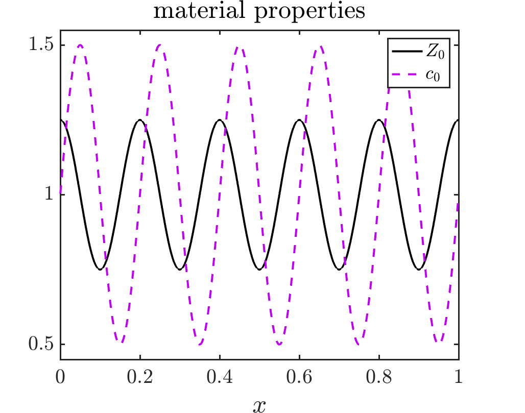
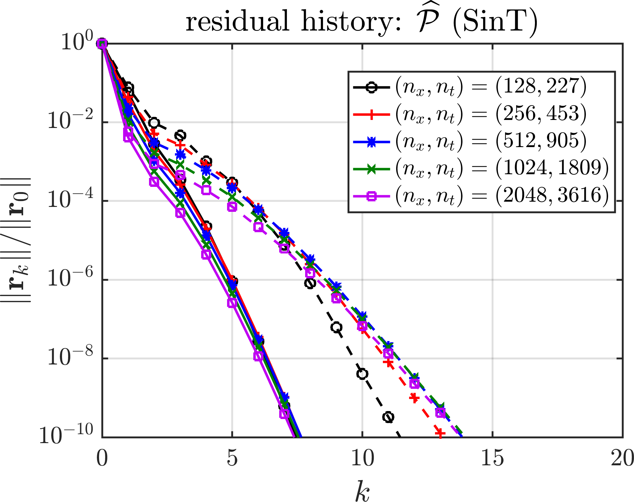
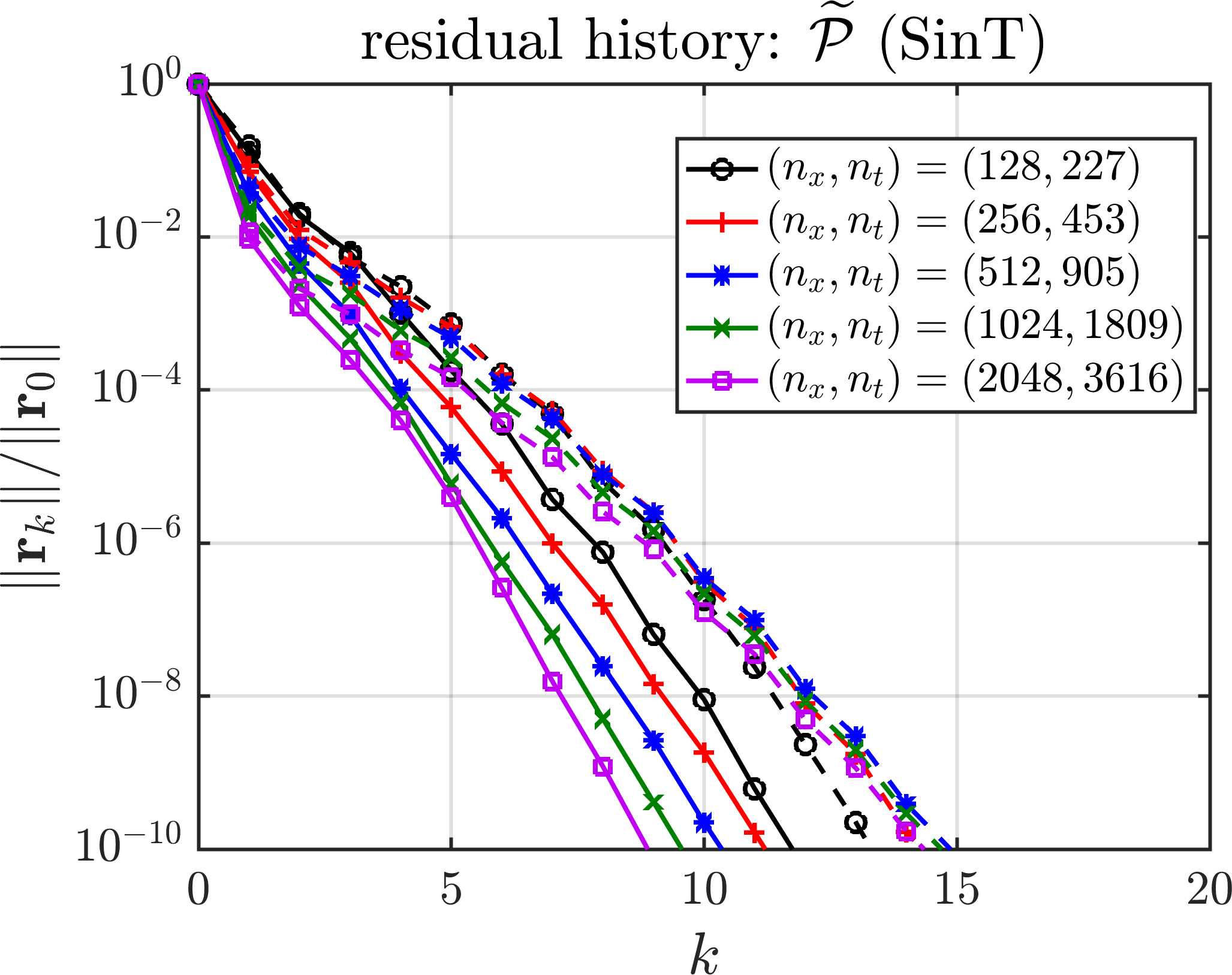
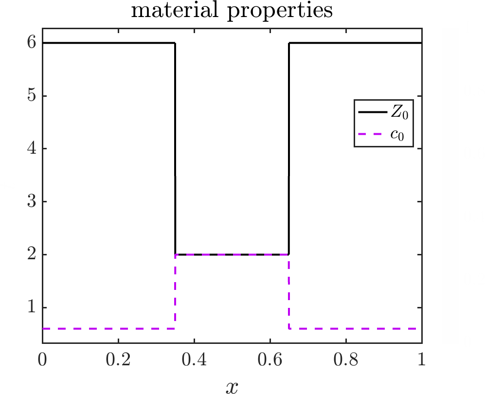
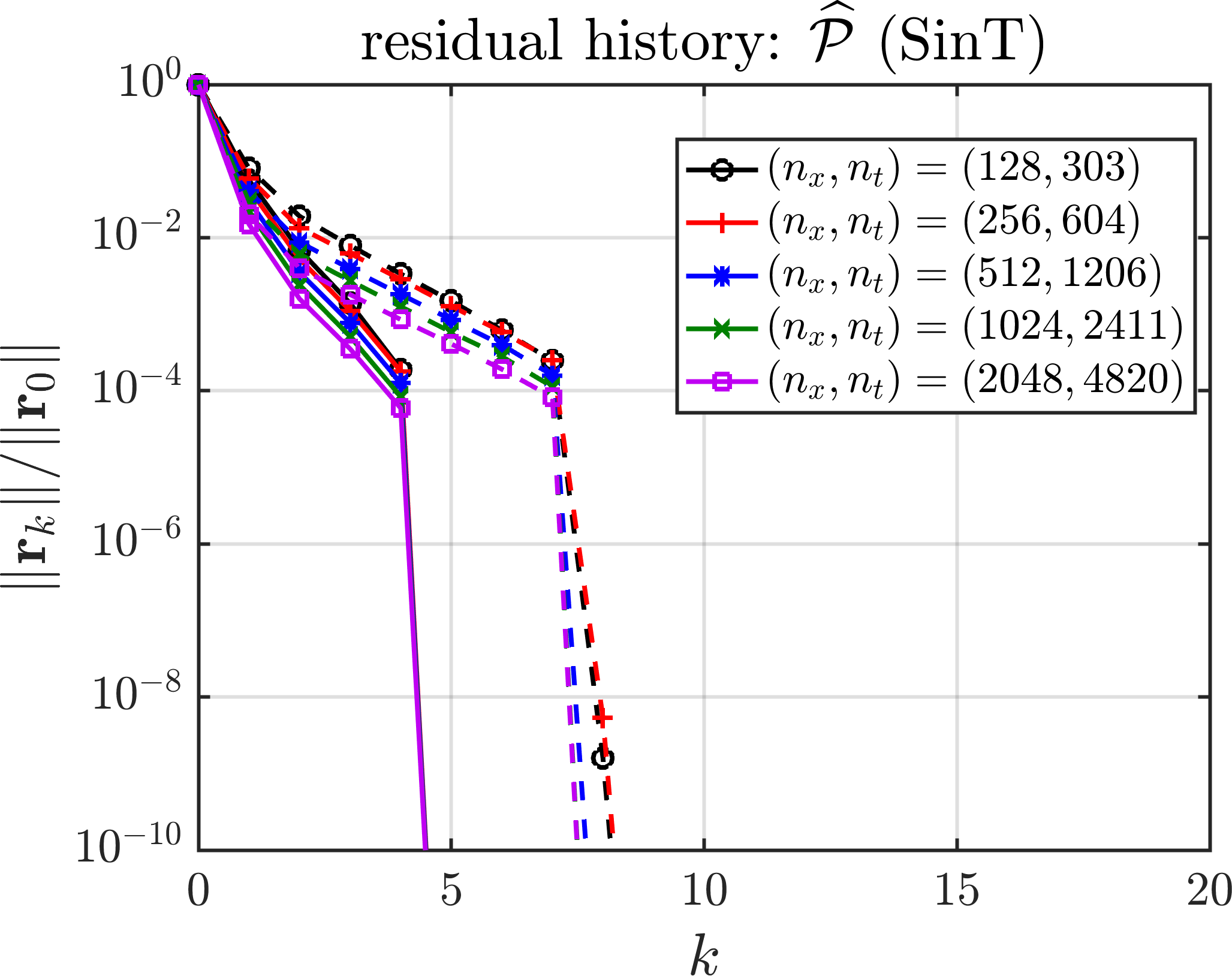
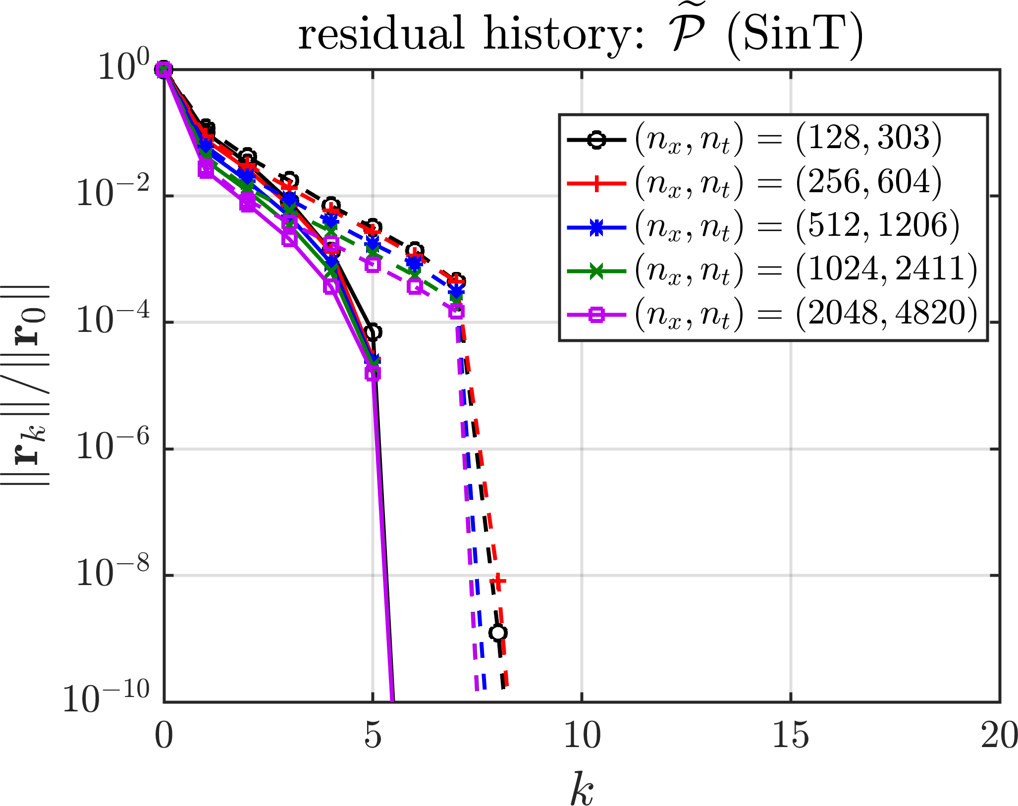
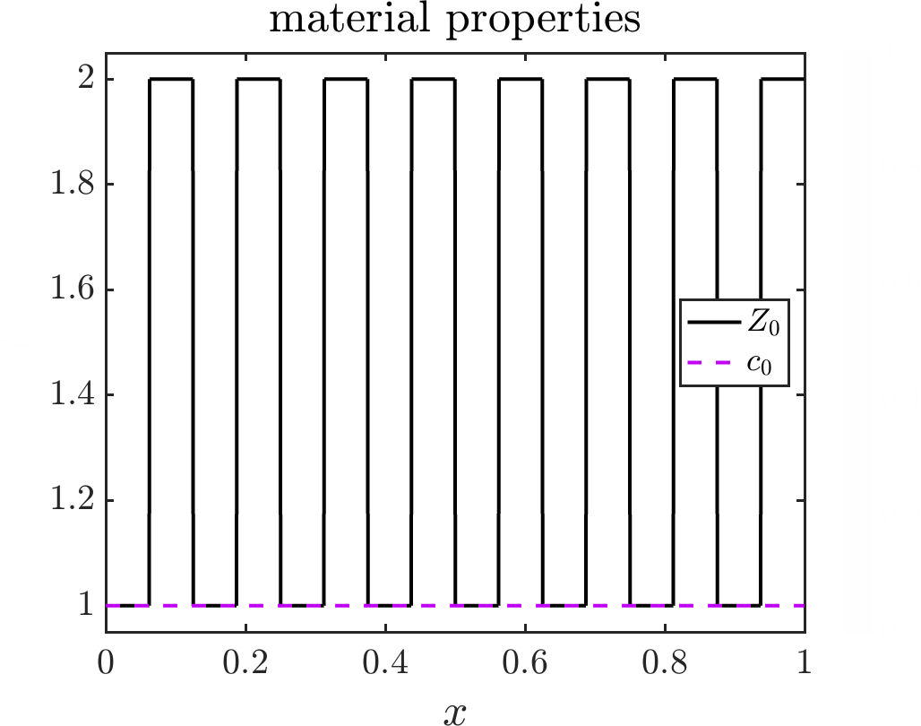
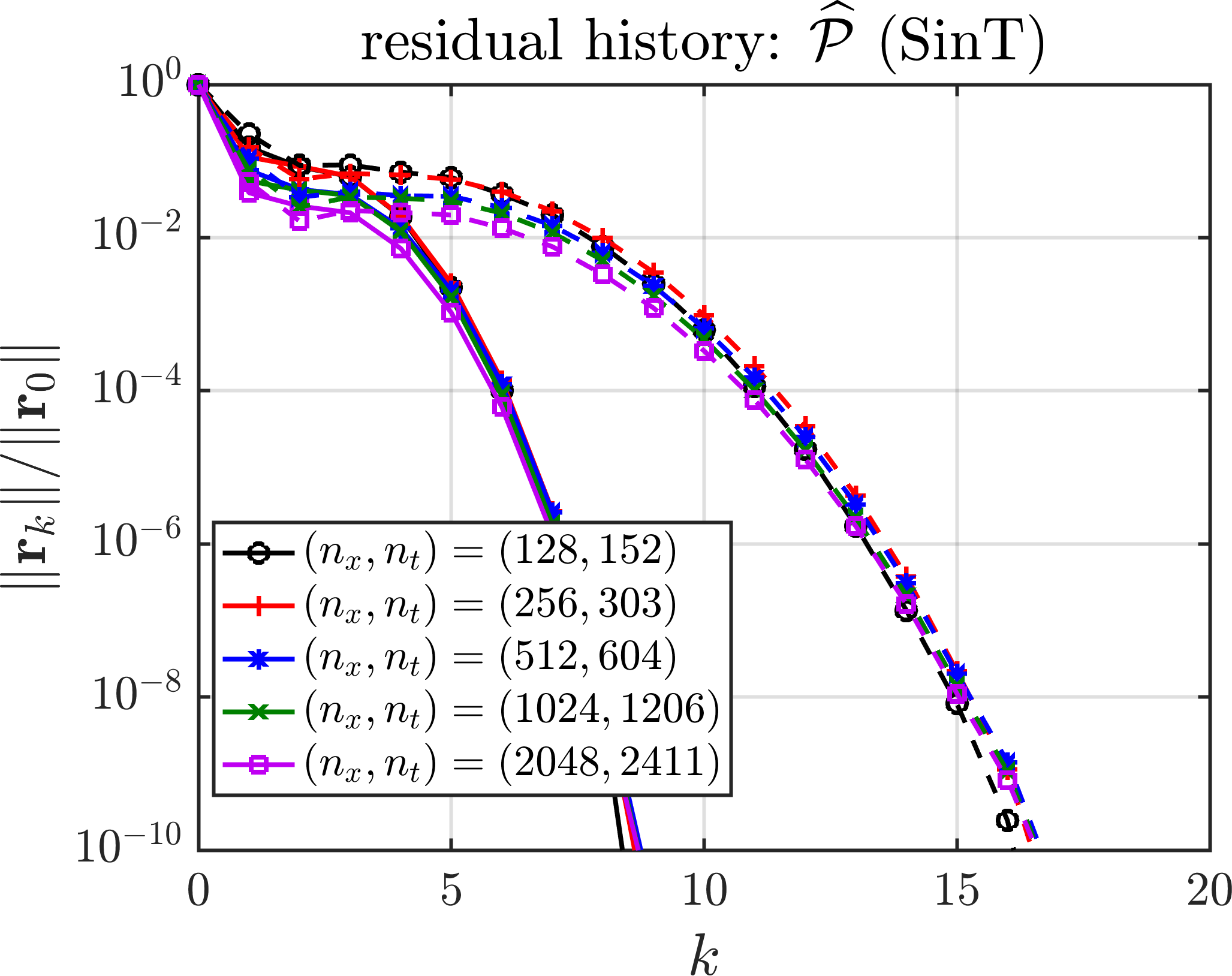
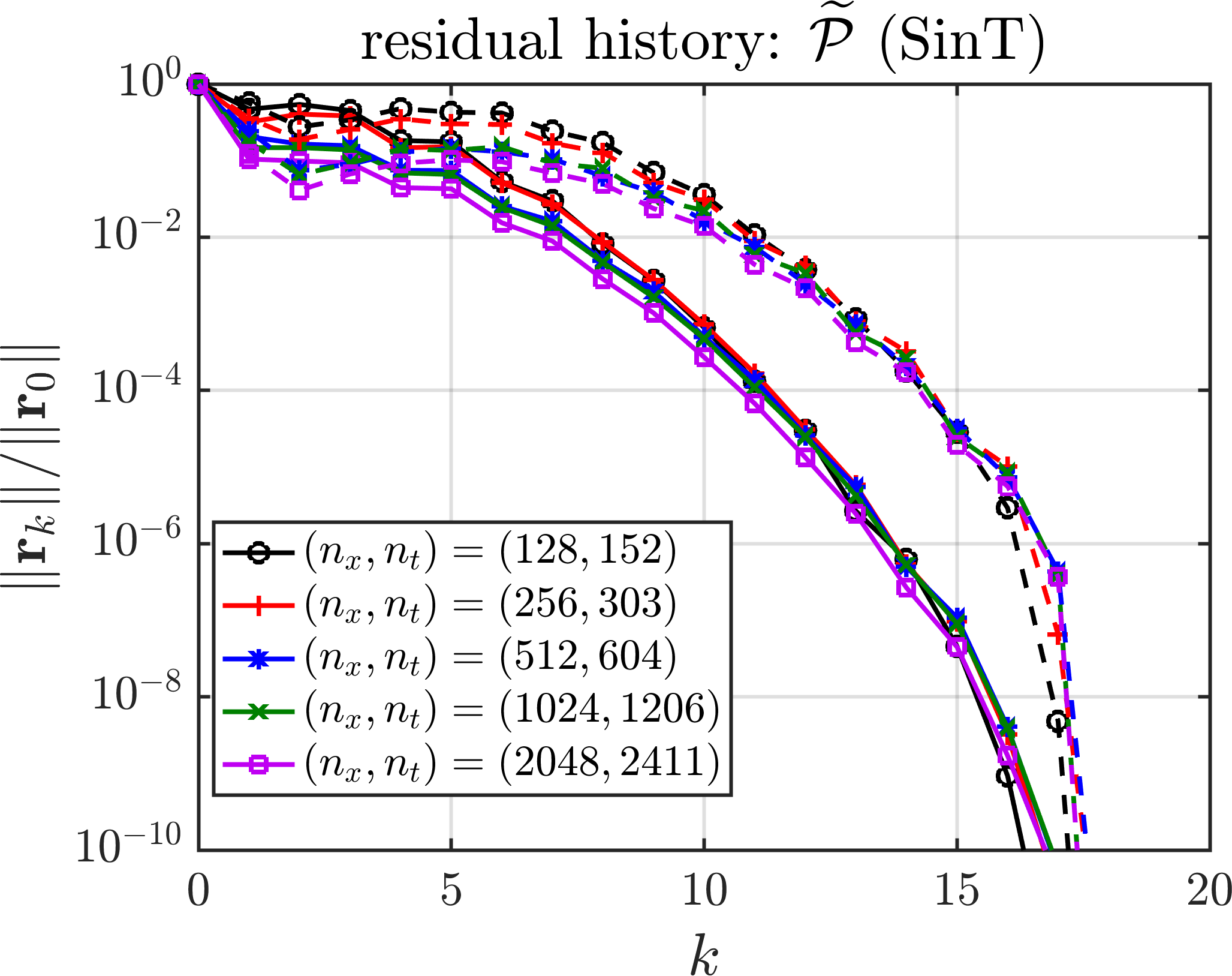
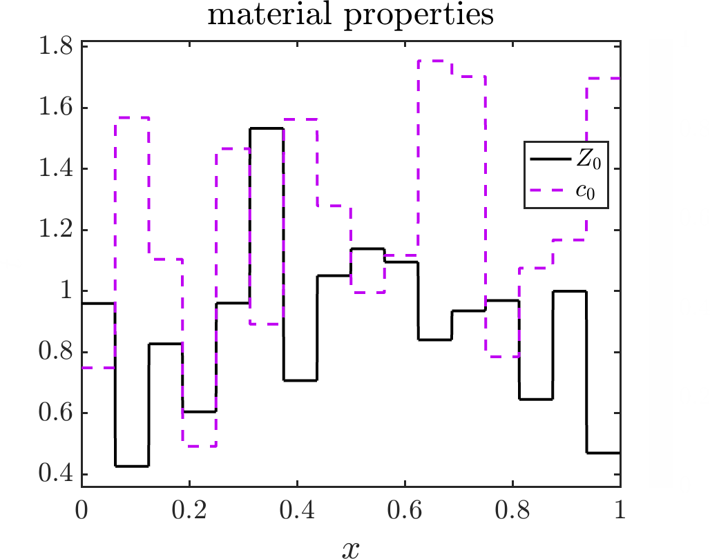
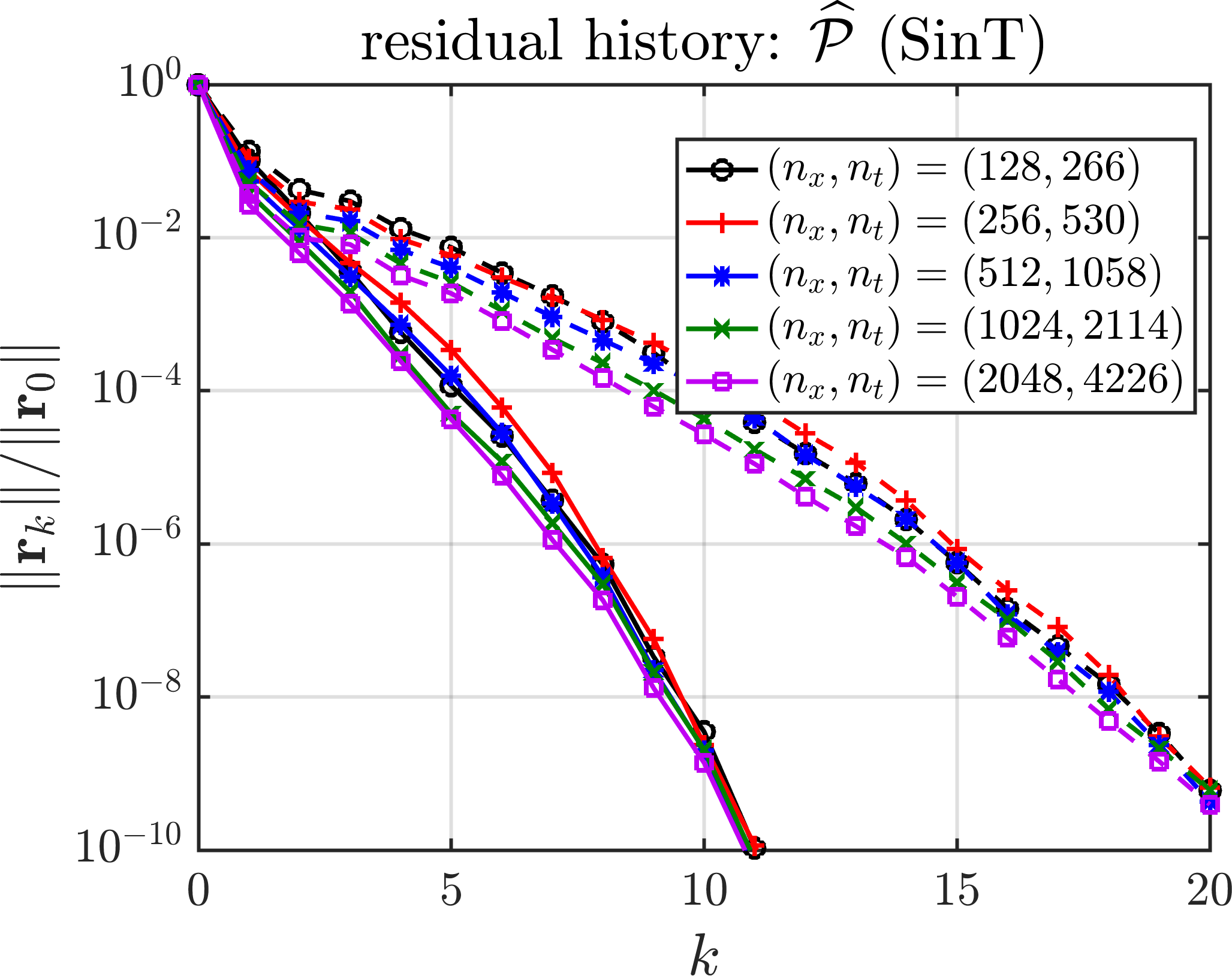
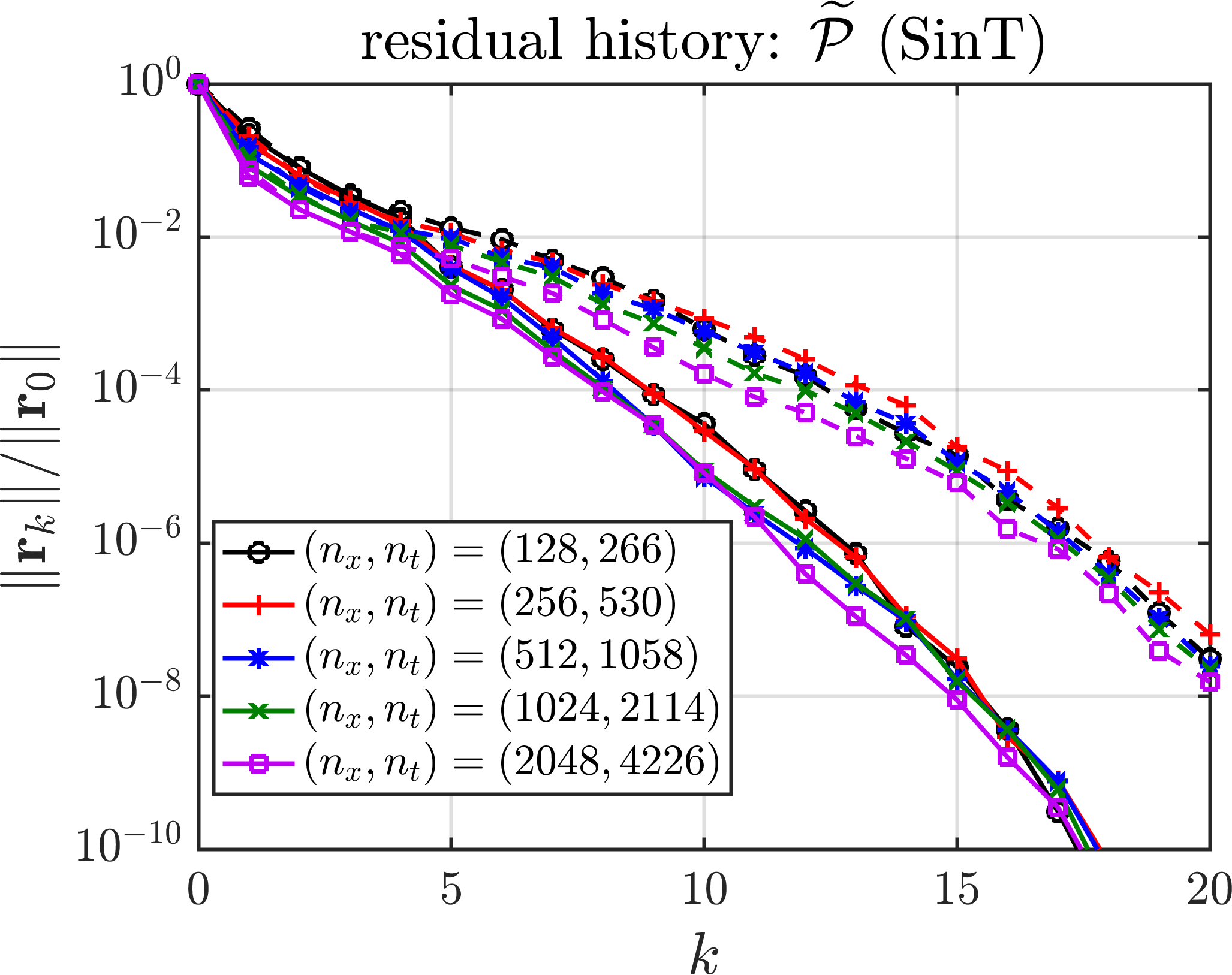
Figure 1: Left: Material properties (27b), (27c), (27d), (27e) ordered from top to bottom. Middle: Residual history using preconditioners $\widehat{{\cal P}}_{L}$ (solid lines) and $\widehat{{\cal P}}_{D}$ (dashed lines) in (23). Right: Residual history using preconditioners $\widetilde{{\cal P}}_{L}$ (solid lines) and $\widetilde{{\cal P}}_{D}$ (dashed lines) in (24) which are based on approximate diagonal blocks. All preconditioners are applied exactly via sequential time-stepping (SinT).

We consider solving (acoustics) on the space-time domain $(x,t)\in(0,1)\times(0,1]$, and subject to the initial conditions

(26) $$u(x,0)=0,\quad p(x,0)=\begin{cases}\tfrac{1}{4}\big{[}7-3\cos(10\pi x-4\pi)\big{]},\quad&x\in(0.4,0.6),\\ 1,\quad&\textrm{else}.\end{cases}$$

We consider five different media, with sound speeds and impedances given by:

(27a) $$c_{0}(x) =1+\tfrac{1}{2}\sin(10\pi x),\quad Z_{0}(x)=1,$$

(27b) $$c_{0}(x) =1+\tfrac{1}{2}\sin(10\pi x),\quad Z_{0}(x)=1+\tfrac{1}{4}\cos(10\pi x),$$

(27c) $$c_{0}(x) =\begin{cases}2,\quad&x\in(0.35,0.65),\\ 0.6,\quad&\textrm{else},\end{cases}\quad\quad Z_{0}(x)=\begin{cases}2,\quad&x\in(0.35,0.65),\\ 6,\quad&\textrm{else},\end{cases}$$

(27d) $$c_{0}(x) =1,\quad\quad Z_{0}(x)=\begin{cases}1,\quad&\textrm{mod}(\lfloor 16x\rfloor,2)=0,\\ 2,\quad&\textrm{else}.\end{cases}$$

(27e) $$c_{0}(x) =\textrm{rand}_{1}(\lfloor 16x\rfloor),\quad\quad Z_{0}(x)=\textrm{rand}_{2}(\lfloor 16x\rfloor).$$

Plots of the material parameters and space-time contours of the associated pressures $p(x,t)$ are shown in the left and middle columns of Fig. 2, respectively—note that the equations in (27e) denote a randomly layered material with 16 layers. For (27a) the characteristic variables decouple globally since $Z_{0}$ is constant, while for all other material parameters they do not. The parameters (27a)–(27c) are used in [1], and (27d) and (27e) are simplified parameters from [34] and [19], respectively.

Shown in Figs. 1 and 2 are two sets of tests corresponding to the exact, sequential-in-time, application of the preconditioners $\widehat{{\cal P}}$ and $\widetilde{{\cal P}}$ in (23) and (24), and their inexact, parallel-in-time application via one MGRIT V-cycle, respectively. In our tests, the time-step size is chosen such that $\delta t=0.85h/\max_{x}c_{0}(x)$. The initial space-time iterate $\bm{q}_{0}$ is chosen with entries drawn randomly from a standard normal distribution, and the convergence metric reported is the 2-norm of the space-time residual of (10) relative to its initial value. The coarsening factor used to create the CF-splitting for the F-relaxation in Line 1 of Algorithm 1 is $m=8$.

Consider first Fig. 1 to understand best-case convergence of the algorithm wherein the preconditioners $\widehat{\cal{P}}$ and $\widetilde{\cal{P}}$ are applied exactly. The simplest material parameters in (27a) are omitted from these tests because the iteration converges to the exact solution in a single iteration due to the characteristic variables globally decoupling. Remarkably, we see that in almost all cases the convergence rate seems independent of problem size. Unsurprisingly, we see that in all cases the lower triangular preconditioner (solid) converges in fewer iterations than the diagonal preconditioner (dashed). We also note there is a mild trend of convergence deteriorating when moving from preconditioners $\widehat{\cal{P}}$ using the true diagonal blocks to preconditioners $\widetilde{\cal{P}}$ using approximate diagonal blocks. This deterioration is most significant for the lower triangular preconditioners in the bottom two rows, corresponding to material parameters (27d), (27e).

  

  

  

  

  

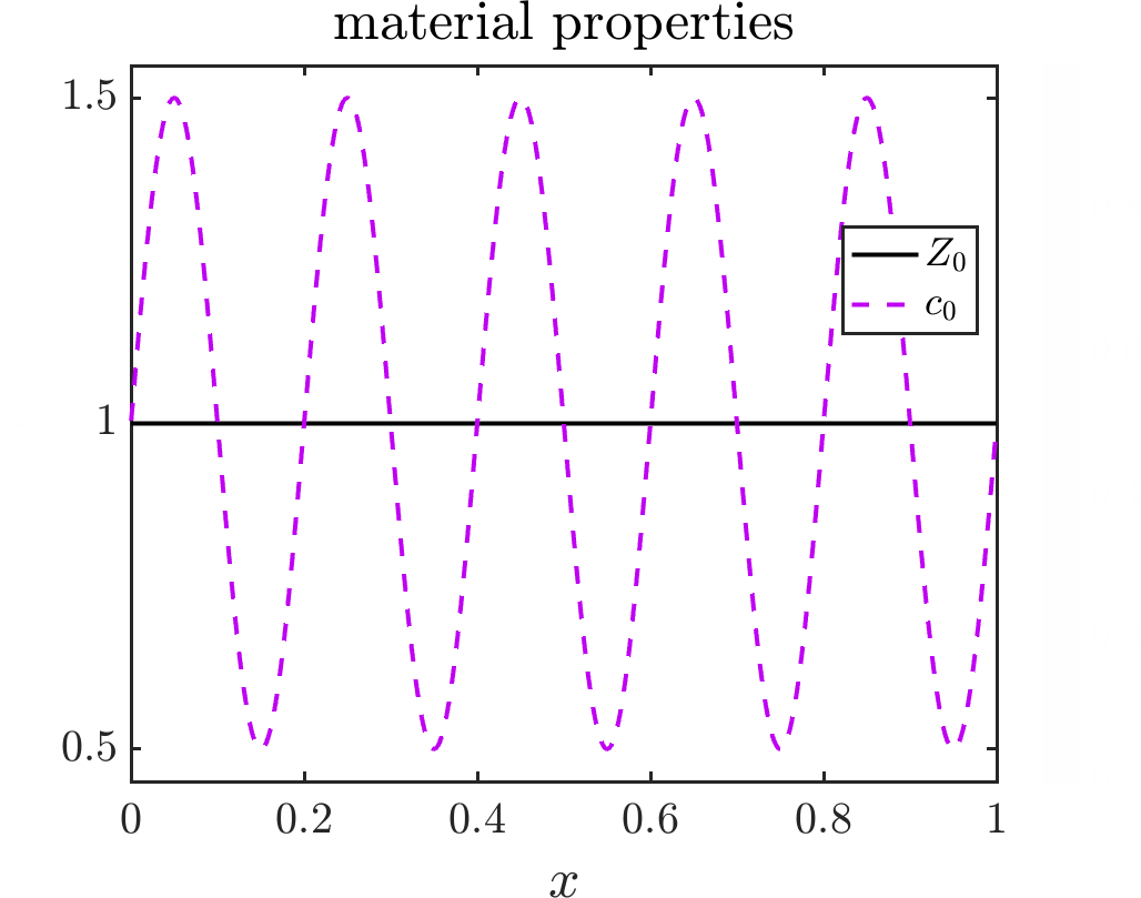
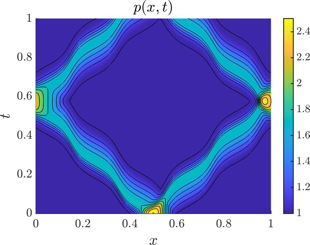
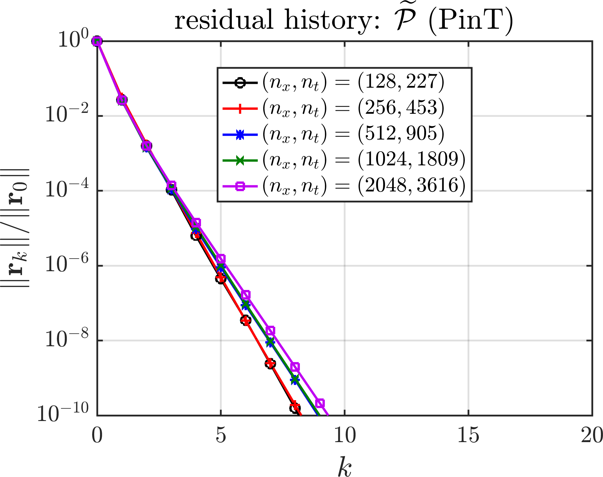
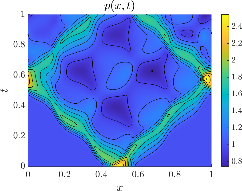
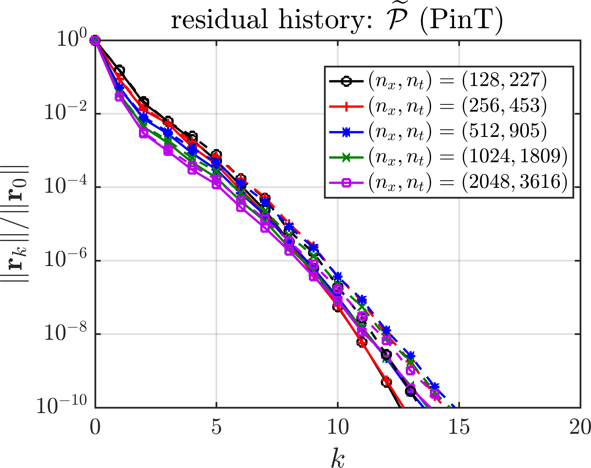
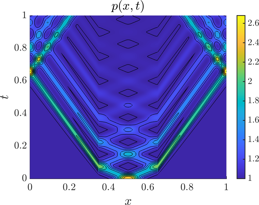
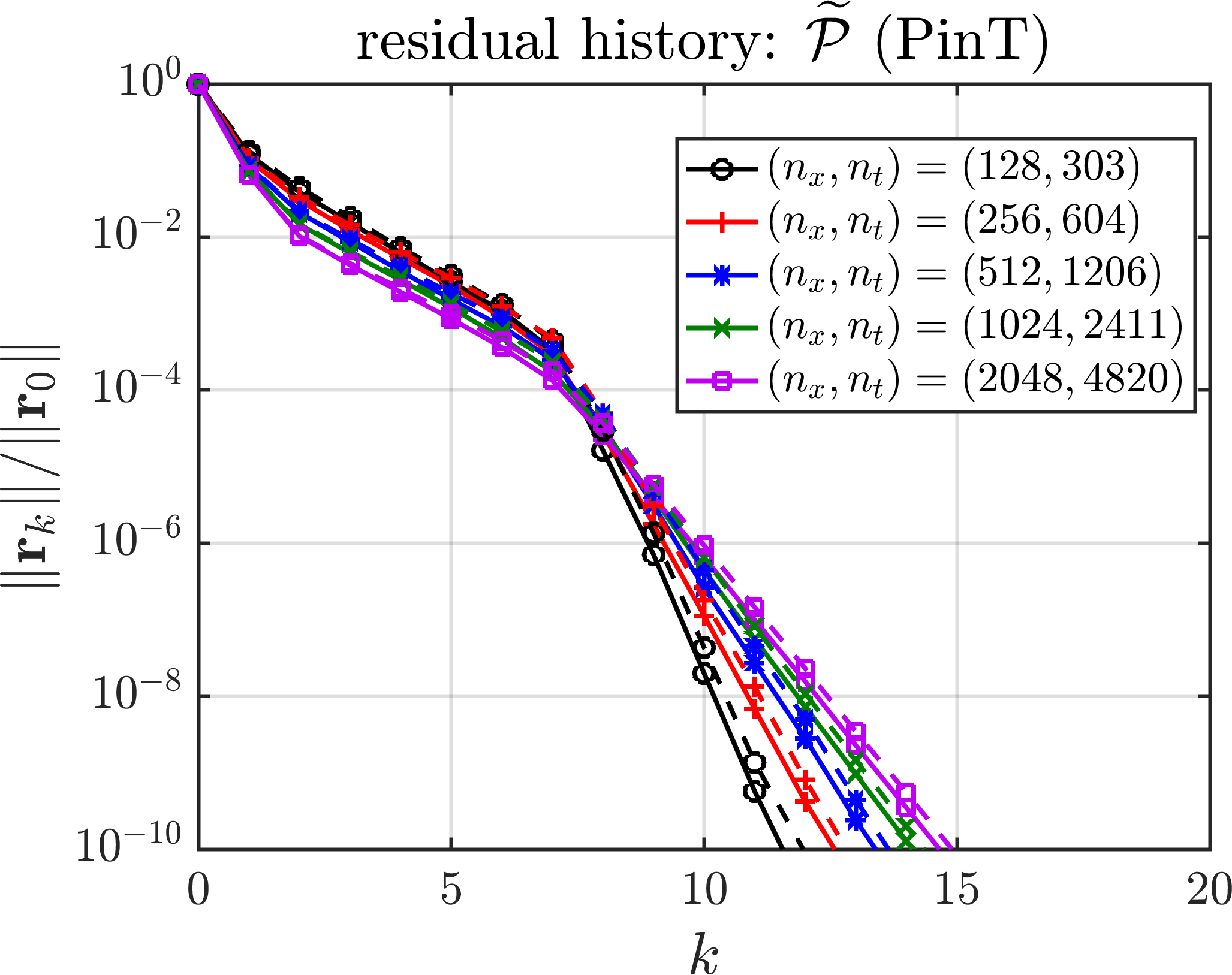
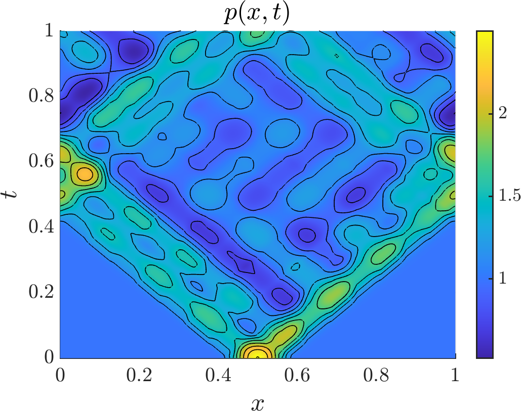
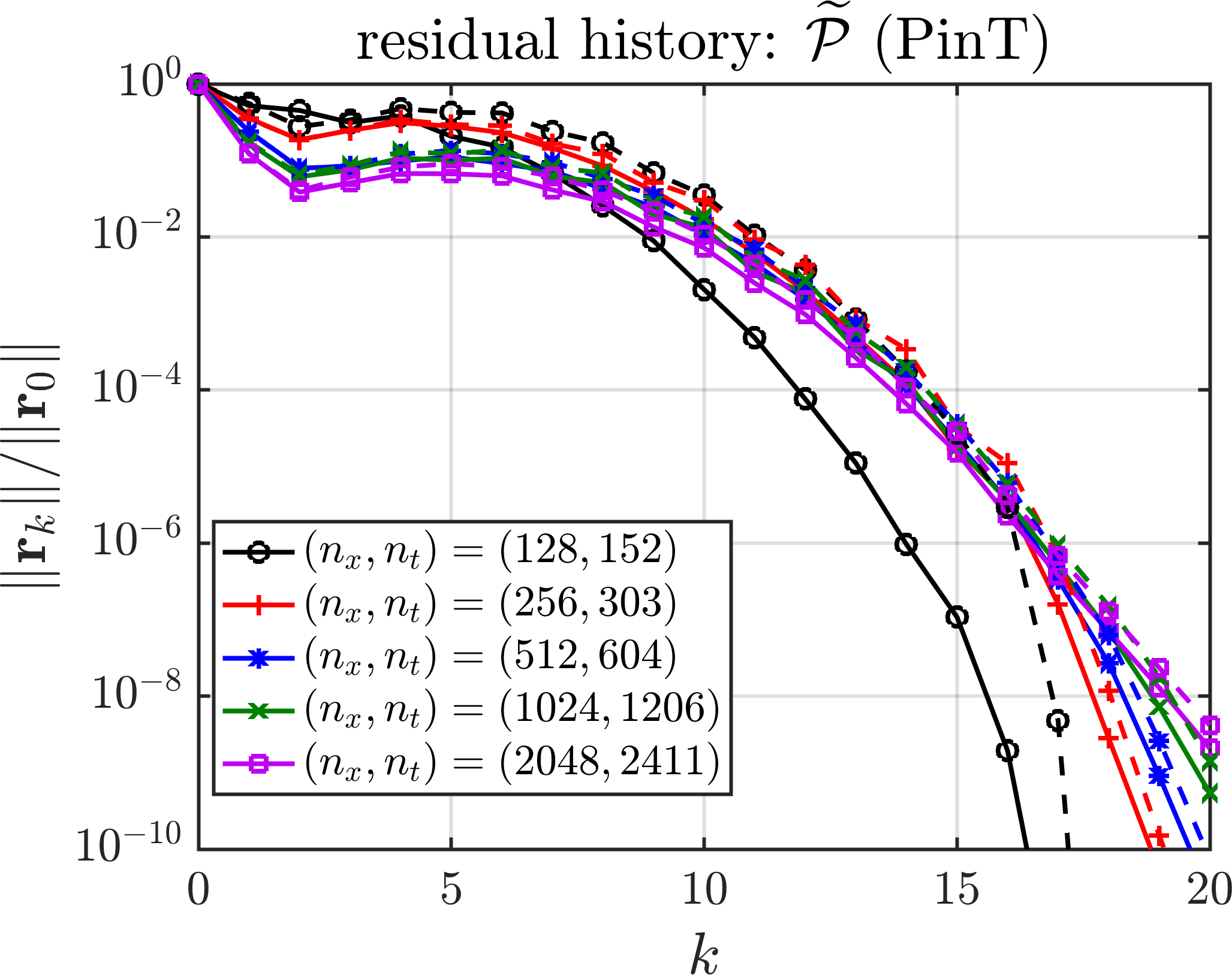
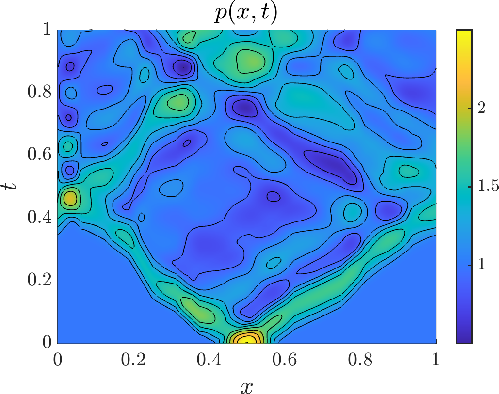
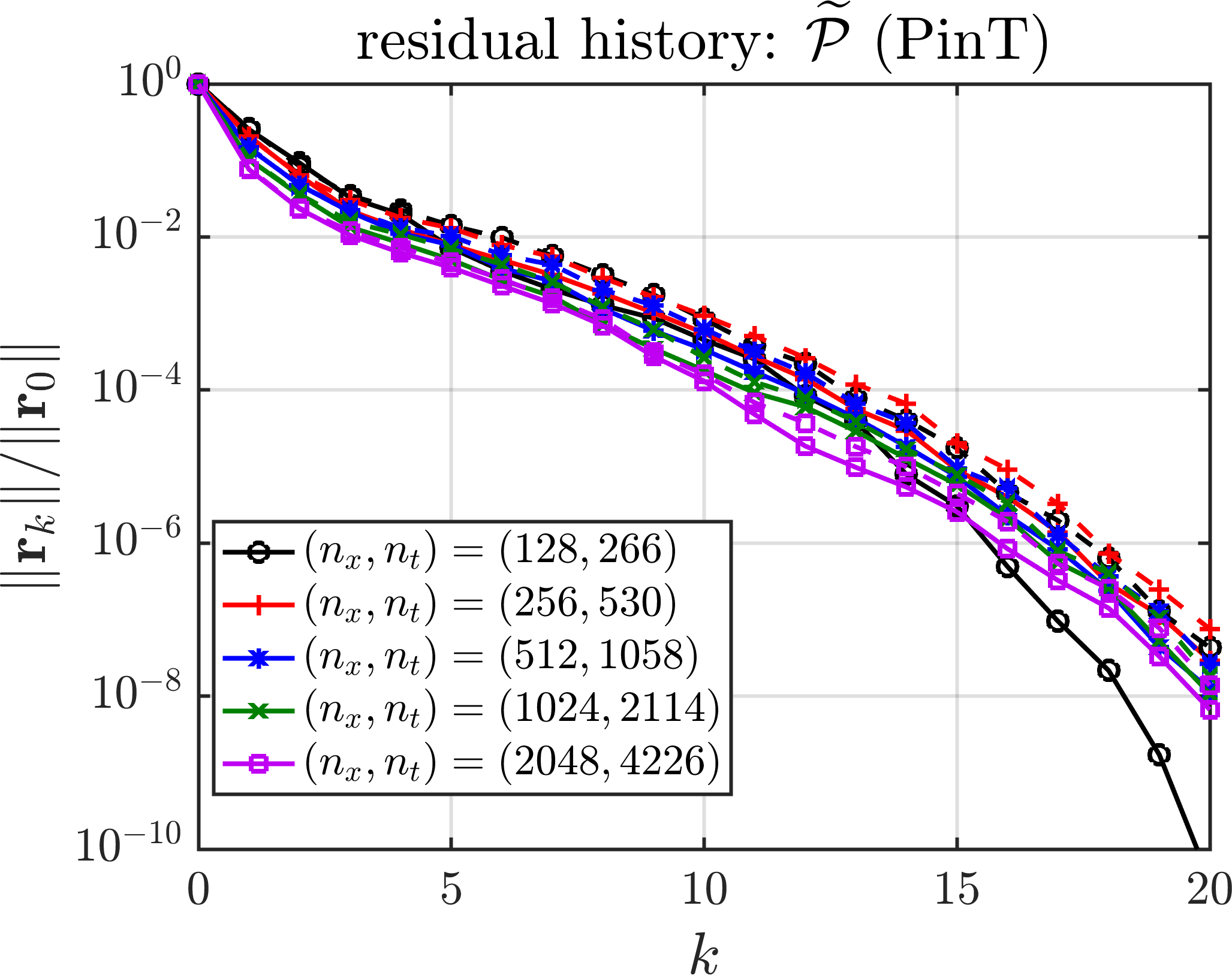
Figure 2: Test problems for the acoustics equations (acoustics). Each of the five rows in the figure corresponds to each of the five material parameters in (27). Left: Material parameters (27). Middle: Space-time contours of the resulting pressure component of the solution vector; note these contours correspond to solves using $n_{x}=2048$. Right: Residual histories when using preconditioners $\widetilde{{\cal P}}$ in (24) with diagonal blocks approximately inverted with a single MGRIT iteration (PinT). Dashed lines correspond to $\widetilde{{\cal P}}_{D}$ and solid lines correspond to $\widetilde{{\cal P}}_{L}$.

Now let us turn our attention to Fig. 2, corresponding to the inexact, parallel-in-time application of the approximate preconditioners $\widetilde{{\cal P}}$ in (24) that employ approximate diagonal blocks $\widetilde{{\cal A}}_{ii}$. In these tests, we apply a single MGRIT V-cycle to approximately invert the Godunov discretizations $\widetilde{{\cal A}}_{11}$ and $\widetilde{{\cal A}}_{22}$. MGRIT coarsens by a factor of $m=8$ on each level, and continues coarsening until fewer than two points in time would result. Each V-cycle uses F-relaxation on the finest level, and FCF-relaxation on all coarser levels. Each V-cycle is initialized with the right-hand side vector. Let $\ell\in\mathbb{N}_{0}$ denote the MGRIT level index, and $\widetilde{\Phi}_{ii}^{m^{\ell}\delta t}$ the time-stepping operator on level $\ell$. Then on coarse levels $\ell>0$ we use a modified semi-Lagrangian discretization [13, 11]

(28) $$\widetilde{\Phi}_{ii}^{m^{\ell}\delta t}=\big{(}I-\operatorname{diag}(\bm{\gamma}_{ii}){\cal D}_{2}\big{)}^{-1}{\cal S}_{ii}^{m^{\ell}\delta t}\approx\prod\limits_{n=0}^{m-1}\widetilde{\Phi}_{ii}^{m^{\ell-1}\delta t}$$

where ${\cal S}_{ii}^{m^{\ell}\delta t}$ is a first-order accurate semi-Lagrangian discretization on grid $\ell$ of linear advection equations with wave-speeds $-c_{0}$ and $+c_{0}$ for $i=1$ and $i=2$, respectively. The vector $\bm{\gamma}_{ii}\in\mathbb{R}^{n_{x}}$ is chosen as in [11] to minimize differences in truncation error of ${\cal S}_{ii}^{m^{\ell}\delta t}$ and $m$ applications of $\widetilde{\Phi}_{ii}^{m^{\ell-1}\delta t}$; the specific coefficients are determined via a simple analysis of the discretizations involved (see our code for specific formulae). The matrix ${\cal D}_{2}\in\mathbb{R}^{n_{x}}$ is the standard second-order accurate Laplacian, $\big{[}{\cal D}_{2}\big{]}_{i}=\left[1,\,-2,\,1\right]/h^{2}$, and the action of the inverse $\big{(}I-\operatorname{diag}(\bm{\gamma}_{ii}){\cal D}_{2}\big{)}^{-1}$ in (28) is approximated with GMRES initialized with a zero vector and iterated until the relative residual is 0.01, or a maximum of 10 iteration is performed.

Considering Fig. 2, we see that the convergence rate of the solver is independent of the mesh resolution. We note that convergence is remarkably fast given the complicated nature of these problems, especially since only a single MGRIT V-cycle is used per inner iteration. Comparing the right column of Fig. 2 with that in Fig. 1, generally speaking, there has been some degradation in convergence when moving from the exact to inexact application of $\widetilde{{\cal P}}^{-1}$. In particular, the lower triangular preconditioner $\widetilde{{\cal P}}_{L}$ loses its advantage over the diagonal preconditioner $\widetilde{{\cal P}}_{D}$ that is present in Fig. 1 where exact inversions were used. Of course, the advantage of $\widetilde{{\cal P}}_{L}$ over $\widetilde{{\cal P}}_{D}$ could be regained through more accurate inner solves, e.g., using two MGRIT V-cycles instead of one; however, more accurate inner solves come at an increased computational cost, so it is unclear whether more accurate inner solves would be beneficial overall. A more definitive answer to these questions would arise from running these solvers on a parallel machine and comparing their time-to-solution. We leave such parallel tests to future work. It is also worth pointing out that in these tests we are significantly oversolving with respect to the discretization error.

4 Conservative nonlinear systems: Introduction and background

We now consider one-dimensional nonlinear conservation law systems of the form

(cons-law) $$\frac{\partial\bm{q}}{\partial t}+\frac{\partial\bm{f}(\bm{q})}{\partial x}=\bm{0},\quad(x,t)\in\Omega\times(0,T],\quad\bm{q}(x,0)=\bm{q}_{\textrm{init}}(x),$$

with solution $\bm{q}=\bm{q}(x,t)=\big{(}q^{1},\ldots,q^{\ell}\big{)}^{\top}\in\mathbb{R}^{\ell}$, and flux function $\bm{f}=\big{(}f^{1},\ldots,f^{\ell}\big{)}^{\top}\in\mathbb{R}^{{\ell}}$; note that “$\ell$” no longer denotes a grid level as in the previous section. The flux Jacobian $A(\bm{q}):=\bm{f}^{\prime}(\bm{q})\in\mathbb{R}^{\ell\times\ell}$ is assumed to have a full set of eigenvectors and real eigenvalues throughout the domain such that (cons-law) is hyperbolic. The flux Jacobian satisfies the decomposition $A=R\Lambda R^{-1}$, where $R=[\bm{r}^{1}\,\ldots\,\bm{r}^{\ell}]$ with right eigenvectors $\bm{r}^{k}\in\mathbb{R}^{\ell}$, and $\Lambda=\operatorname{diag}(\lambda^{1},\ldots,\lambda^{\ell})$, with eigenvalues ordered from smallest to largest, $\lambda^{1}\leq\lambda^{2}\ldots\leq\lambda^{\ell}$.

Numerical results later in Section 5.4 consider two equation systems of the form (cons-law). The first such system is the 1D shallow water equations [34, Chapter 13]:

(shallow-water) $$\frac{\partial}{\partial t}\begin{bmatrix}h\\ hu\end{bmatrix}+\frac{\partial}{\partial x}\begin{bmatrix}hu\\ hu^{2}+\tfrac{1}{2}gh^{2}\end{bmatrix}=\bm{0},\quad g\equiv\textrm{constant}.$$

Here, $h$ is the water height, and $u$ is its velocity, and we set $g=1$. The second model problem is the 1D Euler equations of gas dynamics [34, Chapter 14]:

(euler) $$\frac{\partial}{\partial t}\begin{bmatrix}\rho\\ \rho u\\ E\end{bmatrix}+\frac{\partial}{\partial x}\begin{bmatrix}\rho u\\ \rho u^{2}+p\\ (E+p)u\end{bmatrix}=\bm{0},$$

closed with the equation of state for an ideal polytropic gas, $E=\frac{p}{\gamma-1}+\frac{1}{2}\rho u^{2},\,\gamma\equiv\textrm{constant}.$ Here $\rho$ is the gas density, $u$ its velocity, $E$ its total energy, $p$ its pressure, and we set $\gamma=7/5$. For completeness, the the decompositions $A=R\Lambda R^{-1}$ for (shallow-water) and (euler) can be found in Supplementary Materials Section SM1.

4.1 Finite-volume discretization

The system (cons-law) is discretized in space on a mesh of $n_{x}$ FV cells of equal width $h$, with the $i$th such cell being $x\in[x_{i-1/2},x_{i+1/2}]$, $i\in\{1,\ldots,n_{x}\}$. The temporal domain $t\in[0,T]$ is discretized with a grid of $n_{t}$ points, $\{t_{n}\}_{n=0}^{n_{t}-1}$, $t_{n}=n\delta t$, with constant spacing $\delta t$. We consider a first-order accurate FV method paired with forward Euler integration in time. Ultimately, this discretization results in the one-step scheme

(29) $$\bm{q}_{i}^{n+1}=\bm{q}_{i}^{n}-\frac{\delta t}{h}\Big{[}\widehat{\bm{f}}_{i+1/2}(\bm{q}^{n})-\widehat{\bm{f}}_{i-1/2}(\bm{q}^{n})\Big{]}=:\big{(}\Phi(\bm{q}^{n})\big{)}_{i}\in\mathbb{R}^{\ell},$$

with $\bm{q}_{i}^{n}$ approximating the average of the solution of (cons-law) in cell $i$ at time $t_{n}$. More generally, we use the notation that if $\bm{\zeta}\in\mathbb{R}^{\ell n_{x}}$ is a stacked vector associated with the spatial mesh, then $\bm{\zeta}_{i}\in\mathbb{R}^{\ell}$ denotes a vector with the components of $\bm{\zeta}$ associated with the $i$th FV cell containing $\ell$ variables. In (29), $\widehat{\bm{f}}_{i+1/2}(\bm{q})$ is the numerical flux function, and in this work is the so-called Roe flux:

(30) $$\widehat{\bm{f}}_{i+1/2}(\bm{q})=\frac{1}{2}\Big{[}\big{(}\bm{f}(\bm{q}_{i+1})+\bm{f}(\bm{q}_{i})\big{)}-\big{|}A^{*}_{i+1/2}(\bm{q})\big{|}\big{(}\bm{q}_{i+1}-\bm{q}_{i}\big{)}\Big{]}\in\mathbb{R}^{\ell}.$$

Here $A^{*}_{i+1/2}=A^{*}_{i+1/2}(\bm{q}_{i},\bm{q}_{i+1})$ is a linearization of the flux Jacobian $A(\bm{q}):=\bm{f}^{\prime}(\bm{q})$ about a specially chosen average between $\bm{q}_{i}$ and $\bm{q}_{i+1}$; this flux originated in [43], and we point the reader to LeVeque [34, Chapter 15.3] for details on constructing it for our model problems, see (shallow-water) and (euler). This matrix has the eigen-decomposition $A^{*}_{i+1/2}=R^{*}_{i+1/2}\Lambda^{*}_{i+1/2}(R^{*}_{i+1/2})^{-1}$, where $R^{*}_{i+1/2}=\big{[}\bm{r}_{i+1/2}^{*,1}\ldots\bm{r}_{i+1/2}^{{*,\ell}}\big{]}$, and $\Lambda^{*}_{i+1/2}=\operatorname{diag}\big{(}\lambda_{i+1/2}^{*,1},\ldots,\lambda_{i+1/2}^{*,\ell}\big{)}$. Furthermore, $\big{|}A^{*}_{i+1/2}\big{|}=R^{*}_{i+1/2}\big{|}\Lambda^{*}_{i+1/2}\big{|}(R^{*}_{i+1/2})^{-1}$. As such, (30) can also be written as:

(31) $$\widehat{\bm{f}}_{i+1/2}(\bm{q})=\frac{1}{2}\Big{[}\big{(}\bm{f}(\bm{q}_{i+1})+\bm{f}(\bm{q}_{i})\big{)}-\sum\limits_{j=1}^{\ell}\alpha_{i+1/2}^{*,j}\big{|}\lambda_{i+1/2}^{*,j}\big{|}\bm{r}_{i+1/2}^{*,j}\Big{]},$$

with coefficients $\{\alpha_{i+1/2}^{*,j}\}_{j=1}^{\ell}$ satisfying $\bm{q}_{i+1/2}^{+}-\bm{q}_{i+1/2}^{-}=\sum_{j=1}^{\ell}\alpha_{i+1/2}^{*,j}\bm{r}_{i+1/2}^{*,j}$. Note the Roe flux adds wave-specific dissipation. We also employ “Harten’s Entropy fix” [34, p. 326], whereby the absolute value $|\lambda^{*,j}_{i+1/2}|$ is replaced with the smoothed absolute value in [34, (15.53)] using smoothing parameter $\delta=10^{-6}$. To maintain a simple notation, we still write the smoothed absolute eigenvalues as $|\lambda^{*,j}_{i+1/2}|$.

5 Conservative nonlinear systems: Parallel-in-time solution

In this section, we consider the parallel-in-time solution of the fully discretized problem

(32) $$\bm{q}^{n+1}=\Phi(\bm{q}^{n}),\quad n=0,1,\ldots,n_{t}-2,$$

corresponding to the FV discretization (29) of the PDE system (cons-law). To this end, let us write (32) as a global, nonlinear residual equation:

(33) $$\bm{r}(\bm{q}):=\bm{b}-{\cal N}(\bm{q})\equiv\begin{bmatrix}\bm{q}^{0}\\ \bm{0}\\ \vdots\\ \bm{0}\end{bmatrix}-\begin{bmatrix}I&\\ -\Phi(\,\cdot\,)&I\\ &\ddots&\ddots\\ &&-\Phi(\,\cdot\,)&I\end{bmatrix}\begin{bmatrix}\bm{q}^{0}\\ \bm{q}^{1}\\ \vdots\\ \bm{q}^{n_{t}-1}\end{bmatrix}=\bm{0}.$$

Here $\bm{q}:=(\bm{q}^{0,\top},\bm{q}^{1,\top},\ldots,\bm{q}^{n_{t}-1,\top})^{\top}\in\mathbb{R}^{{\ell}n_{x}n_{t}}$, ${\cal N}\colon\mathbb{R}^{{\ell}n_{x}n_{t}}\to\mathbb{R}^{{\ell}n_{x}n_{t}}$ is the nonlinear space-time discretization operator, and $\bm{b}\in\mathbb{R}^{{\ell}n_{x}n_{t}}$ contains the initial data.

Here we solve (33) using a residual correction scheme based on that developed in [12] for scalar nonlinear hyperbolic PDEs. A summary of the procedure is given in Algorithm 2, wherein $\bm{q}_{k}$ is an iterative approximation of $\bm{q}$ with iteration index $k$. This scheme combines an outer iteration based on a global linearization with an inner iteration for the associated linearized systems. Note that this algorithm requires a CF-splitting defined by some integer $m>1$, and that the F-relaxation in Line 2 is equivalent to the regular F-relaxation that MGRIT uses for nonlinear problems [32]. The primary step in the algorithm is the solution of a linearized problem ${\cal A}_{k}\bm{e}_{k}^{\rm lin}=\bm{r}_{k}$ with space-time matrix ${\cal A}_{k}$ given by

(34) $${\cal A}_{k}=\begin{bmatrix}&I\\ &-\Phi^{\rm lin}(\bm{q}_{k}^{0})&I\\ &&\ddots&\ddots\\ &&&-\Phi^{\rm lin}(\bm{q}_{k}^{n_{t}-2})&I\end{bmatrix}\in\mathbb{R}^{{\ell}n_{x}n_{t}\times{\ell}n_{x}n_{t}}.$$

In Algorithm 2 there is an option to invert ${\cal A}_{k}$ directly with sequential time-stepping or approximately with the characteristic-based block preconditioner from Algorithm 1. Ultimately we are interested in the latter option since it allows for a parallel-in-time implementation, but, importantly, the direct inversion option allows for us to understand best-case convergence of the outer preconditioned nonlinear residual correction iteration.

Input: Initial iterate $\bm{q}_{0}\approx\bm{q}$; number of iterations maxit; number of inner iterations inner-it

$k\leftarrow 0$;

  // Iteration counter

Output: Approximate solution $\bm{q}_{k}\approx\bm{q}$

1 while $k<\mathtt{maxit}$ do

       ${\bm{q}}_{k}\leftarrow\textrm{relax on }{\cal N}(\bm{q}_{k})\approx\bm{b}$;

        // Nonlinear F-relaxation

       ${\bm{r}}_{k}\leftarrow\bm{b}-{\cal N}({\bm{q}}_{k})$;

        // Compute residual

2       if exact linear solve then

             /* Directly compute linearized error via time-stepping; sequential-in-time */

3             ${\bm{e}}_{k}^{\rm lin}\leftarrow{\cal A}_{k}^{-1}{\bm{r}}_{k}$

4       else

             /* Approximate error using inner-it iterations of char.-based block preconditioning in Algorithm 1; may be solved parallel-in-time */

             ${\bm{e}}_{k}^{\rm lin}\leftarrow\textrm{char-based-block-prec}({\cal A}_{k},{\bm{e}}_{k}^{\rm lin},{\bm{r}}_{k},$inner-it);

              // Need to initialize ${\bm{e}}_{k}^{\rm lin}$

5            

      $\bm{q}_{k+1}\leftarrow{\bm{q}}_{k}+{\bm{e}}_{k}^{\rm lin}$;

        // Compute new iterate

       $k\leftarrow k+1$;

        // Increment iteration counter

6      

Algorithm 2 Preconditioned residual correction scheme for (33).

Next in Section 5.1, we develop an expression for $\Phi^{\rm lin}(\bm{q}_{k}^{n})$ in (34), and then in Sections 5.2 and 5.3 we discuss characteristic-variable block preconditioning for the linearized problems. We conclude with numerical results in Section 5.4.

5.1 The linearized time-stepping operator

Considering the form of $\Phi$ in (29), its Jacobian exists everywhere because the dissipation matrix (the only potentially problematic term) $|A^{*}_{i+1/2}|$ is based on a smoothed absolute value function. In [12], in the context of scalar PDEs, non-differentiability of $\Phi$ arose due to non-smoothness of the dissipation coefficient in a local Lax–Friedrichs numerical flux, which uses a non-smoothed absolute value. Yet, we were able to develop effective $\Phi^{\rm lin}$ in [12] by freezing the dissipation coefficient in the numerical flux while differentiating $\Phi$. This also led to tractable methods with manageable computational costs. To develop a tractable expression for $\Phi^{\rm lin}$ in the present setting, we apply this same idea leading to the following approximate Jacobian:

(35) $$\Phi^{\rm lin}(\bm{q}_{k}^{n})=\Big{[}\nabla_{\bm{q}_{k}^{n}}\Phi(\bm{q}_{k}^{n})\Big{]}_{|A^{*}(\bm{q}_{k}^{n})|},$$

where this notation denotes holding $|A^{*}(\bm{q}_{k}^{n})|$ constant when differentiating $\Phi$ in (29).

To simplify notation, let us drop the iteration index $k$ henceforth. Consider that in Algorithm 2 we need to solve ${\cal A}\bm{e}=\bm{r}$. Given the sparsity structure of ${\cal A}$ in (34) it becomes apparent that we need to know how to compute the action of $\Phi^{\rm lin}(\bm{q}^{n})$ on some (error) vector $\bm{e}^{n}\in\mathbb{R}^{\ell n_{x}}$. In particular, it suffices for us to understand how to compute this action in cell $i$:

(36) $$\big{(}\Phi^{\rm lin}(\bm{q}^{n})\bm{e}^{n}\big{)}_{i}=\Big{(}\Big{[}\nabla_{\bm{q}^{n}}\Phi(\bm{q}^{n})\Big{]}_{|A^{*}(\bm{q}^{n})|}\bm{e}^{n}\Big{)}_{i}=\Big{[}\nabla_{\bm{q}^{n}}\big{(}\Phi(\bm{q}^{n})\big{)}_{i}\Big{]}_{|A^{*}(\bm{q}^{n})|}\bm{e}^{n}\in\mathbb{R}^{\ell},$$

with $\big{(}\Phi(\bm{q}^{n})\big{)}_{i}$ defined in (29), and $\Big{[}\nabla_{\bm{q}^{n}}\big{(}\Phi(\bm{q}^{n})\big{)}_{i}\Big{]}_{|A^{*}(\bm{q}^{n})|}\in\mathbb{R}^{\ell\times\ell n_{x}}$ being its approximate Jacobian. Differentiating (29) in the direction of $\bm{e}^{n}$ we find

(37) $$\big{(}\Phi^{\rm lin}(\bm{q}^{n})\bm{e}^{n}\big{)}_{i}=\Big{[}\nabla_{\bm{q}^{n}}\big{(}\Phi(\bm{q}^{n})\big{)}_{i}\Big{]}_{|A^{*}(\bm{q}^{n})|}\bm{e}^{n}=\bm{e}^{n}_{i}-\frac{\delta t}{h}\Big{[}\widehat{\bm{f}}_{i+1/2}^{\textrm{lin},n}-\widehat{\bm{f}}_{i-1/2}^{\textrm{lin},n}\Big{]},$$

where, by the chain rule, we have $\widehat{\bm{f}}_{i+1/2}^{\textrm{lin},n}:=\Big{[}\nabla_{\bm{q}^{n}}\widehat{\bm{f}}_{i+1/2}(\bm{q}^{n})\Big{]}_{|A^{*}(\bm{q}^{n})|}\bm{e}^{n}$. Using (30) to compute this directional derivative gives

(38) $$\widehat{\bm{f}}_{i+1/2}^{\textrm{lin},n}=\frac{1}{2}\Big{[}\Big{(}A(\bm{q}_{i+1}^{n})\bm{e}^{n}_{i+1}+A(\bm{q}_{i}^{n})\bm{e}^{n}_{i}\Big{)}-\big{|}A^{*}_{i+1/2}(\bm{q}^{n})\big{|}\big{(}\bm{e}_{i+1}^{n}-\bm{e}_{i}^{n}\big{)}\Big{]}\in\mathbb{R}^{\ell},$$

recalling the shorthand $A(\bm{q}):=\bm{f}^{\prime}(\bm{q})$ for the flux Jacobian.

Observe that the linearized time-stepping operator (37), paired with the linearized flux (38), has a structure that is almost identical to the nonlinear time-stepping operator (29), paired with the nonlinear flux (30). That is, (37) is the time-stepping operator of a first-order FV discretization of the linear system of conservation laws

(39) $$\frac{\partial\bm{e}_{k}}{\partial t}+\frac{\partial}{\partial x}\big{(}A(\bm{q}_{k})\bm{e}_{k}\big{)}=\bm{0},\quad(x,t)\in\Omega\times(0,T],$$

with $\bm{q}_{k}$ the current approximation to the solution $\bm{q}$ of the nonlinear space-time system (33) (the nonlinear iteration index $k$ is included here for clarity). Specifically, if we define the linearized flux function $\bm{f}^{\textrm{lin}}(\bm{e}):=A(\bm{q}_{k})\bm{e}$, then the linearized discretization (37) arises from applying a first-order FV discretization to (39) with a Roe-like flux based on $\bm{f}^{\textrm{lin}}(\bm{e})$. This scenario is a direct systems generalization of the situation in [12] where the linearized problem is a scalar conservation law based on a linearization of the flux in the underlying nonlinear PDE. This realization allows us to compute truncation error corrections for semi-Lagrangian coarse-grid schemes that are crucial for efficient MGRIT preconditioning when inexactly applying Line 2 of Algorithm 2.

5.2 The inner linearized iteration

We now discuss solving the linearized systems in Algorithm 2 using characteristic-variable block preconditioning. Throughout this section we drop the nonlinear iteration index $k$ for readability, but, where convenient to do so, we add “0” subscripts to quantities associated with the flux Jacobian to remind the reader that it is based on $\bm{q}_{k}\approx\bm{q}$; that is, $A_{0}:=A(\bm{q}_{k})$.

Our approach for solving the linearized system ${\cal A}_{0}\bm{e}=\bm{r}$ is based on that developed for the acoustics system in Section 3. However, there are a few key differences: (i) the PDE system (39) is ${\ell}$-dimensional, while (acoustics) is two-dimensional; (ii) the PDE system (39) is in conservative form, while (acoustics) is in non-conservative form; (iii) the coefficient matrix $A_{0}:=A(\bm{q}_{k})$ in (39) varies in both space and time, while that in (acoustics) varies in space only. Despite these key differences, Algorithm 1 can be used without modification (modulo changes in notation) to approximately solve ${\cal A}_{0}\bm{e}=\bm{r}$. The remainder of this section discusses transforming to characteristic variables, and block preconditioners.

To gain insight into the characteristic variables at the discrete level, we first consider them at the PDE level. To re-express the linearized PDE (39) in characteristic variables $\widehat{\bm{e}}:=R_{0}^{-1}\bm{e}$—recall that characteristic-space quantities are denoted with a hat—, multiply the PDE from the left by $R_{0}^{-1}$ to get

(40) $$\bm{0}=R_{0}^{-1}\left[\frac{\partial}{\partial t}\big{(}R_{0}\widehat{\bm{e}}\big{)}+\frac{\partial}{\partial x}\big{(}R_{0}\Lambda_{0}\widehat{\bm{e}}\big{)}\right]\approx\frac{\partial\widehat{\bm{e}}}{\partial t}+\frac{\partial}{\partial x}\big{(}\Lambda_{0}\widehat{\bm{e}}\big{)}\quad\textrm{when $R_{0}$ is slowly varying},$$

with $A_{0}=R_{0}\Lambda_{0}R_{0}^{-1}$. A pertinent question is to what extent the eigenvectors $R_{0}$ of the flux Jacobian may be slowly varying. In general, we cannot assume they vary slowly; however, in practice, this may be a reasonable approximation for many problems. That is, even though (cons-law) admits solutions with shocks—across which $R_{0}$ may change discontinuously—, in practice they are typically limited in number, contained in isolated regions of space-time, and away from these shocked regions, the solution may be smoothly and slowly varying. For example, in the context of motivating linearized Riemann solvers, LeVeque [34, p. 316] writes “… The solution to a conservation law typically consists of at most a few isolated shock waves or contact discontinuities separated by regions where the solution is smooth. In these regions, the variation in $\bm{q}$ from one grid cell to the next has $\|\bm{q}_{i}-\bm{q}_{i-1}\|={\cal O}(h)$ and the Jacobian matrix is nearly constant, $\bm{f}^{\prime}(\bm{q}_{i-1})\approx\bm{f}^{\prime}(\bm{q}_{i})$.”

5.3 Constructing $\widehat{{\cal P}}$ and $\widetilde{{\cal P}}$

We now consider characteristic variables at the discrete level. Recall from Section 5.1 that the global linearized system is

(41) $${\cal A}_{0}\bm{e}=\bm{r},\quad\textrm{or}\quad\bm{e}^{n+1}=\Phi_{0}^{n}\bm{e}^{n}+\bm{r}^{n+1},\quad n=0,\ldots,n_{t}-2,$$

where we now use the shorthand $\Phi^{n}_{0}:=\Phi^{\textrm{lin}}(\bm{q}^{n})$ for readability. To transform this discretized system to characteristic variables we need to introduce the discretized left and right eigenvector matrices $({\cal R}_{0}^{n})^{-1}$ and ${\cal R}_{0}^{n}\in\mathbb{R}^{\ell n_{x}\times\ell n_{x}}$, respectively. These are $\ell\times\ell$ block matrices where the $ij$th block is a diagonal matrix corresponding to the values of the $ij$th element of $(R_{0}^{n})^{-1}$ and $R_{0}^{n}$, respectively, over the grid points, i.e., these matrices generalize those in (13) that discretize the eigenvectors of the flux Jacobian in (acoustics). Multiplying the $n$th equation in (41) on the left by $({\cal R}_{0}^{n+1})^{-1}$ we get the characteristic-space residual equation

(42) $$\begin{split}\widehat{\bm{e}}^{n+1}&=\widehat{\Phi}_{0}^{n}\widehat{\bm{e}}^{n}+\widehat{\bm{r}}^{n+1},\quad n=0,\ldots,n_{t}-2,\quad\textrm{where},\quad\quad\widehat{\bm{e}}^{n}:=({\cal R}_{0}^{n})^{-1}{\bm{e}}^{n},\\ \widehat{\Phi}_{0}^{n}&:=({\cal R}_{0}^{n+1})^{-1}{\Phi}_{0}^{n}{\cal R}_{0}^{n}=\begin{bmatrix}\widehat{\Phi}_{0,11}^{n}&\ldots&\widehat{\Phi}_{0,1\ell}^{n}\\ \vdots&\ddots&\vdots\\ \widehat{\Phi}_{0,\ell 1}^{n}&\ldots&\widehat{\Phi}_{0,\ell\ell}^{n}\end{bmatrix},\quad\widehat{\bm{r}}^{n}:=({\cal R}_{0}^{n})^{-1}{\bm{r}}^{n}.\end{split}$$

Re-ordering this system to be blocked by characteristic variable gives:

(43) $$\widehat{{\cal A}}_{0}\widehat{\bm{e}}=\widehat{\bm{r}},\quad\textrm{or}\quad\begin{bmatrix}\widehat{{\cal A}}_{0,11}&\ldots&\widehat{{\cal A}}_{0,1\ell}\\ \vdots&\ddots&\vdots\\ \widehat{{\cal A}}_{0,\ell 1}&\ldots&\widehat{{\cal A}}_{0,\ell\ell}\end{bmatrix}\begin{bmatrix}\widehat{\bm{e}}^{1}\\ \vdots\\ \widehat{\bm{e}}^{\ell}\end{bmatrix}=\begin{bmatrix}\widehat{\bm{r}}^{1}\\ \vdots\\ \widehat{\bm{r}}^{\ell}\end{bmatrix},$$

where the blocks $\widehat{{\cal A}}_{0,ii},\widehat{{\cal A}}_{0,ij}\in\mathbb{R}^{n_{x}n_{t}\times n_{x}n_{t}}$, $j\neq i$, are given by

(44) $$\widehat{{\cal A}}_{0,ii}=\begin{bmatrix}I\\ -\widehat{\Phi}^{0}_{0,ii}&I\\ &\ddots&\ddots\\ &&-\widehat{\Phi}^{n_{t}-1}_{0,ii}&I\end{bmatrix},\quad\widehat{{\cal A}}_{0,ij}=\begin{bmatrix}0\\ -\widehat{\Phi}^{0}_{0,ij}&0\\ &\ddots&\ddots\\ &&-\widehat{\Phi}^{n_{t}-1}_{0,ij}&0\end{bmatrix}.$$

We now propose an $\ell\times\ell$ block preconditioner $\widehat{{\cal P}}$ by truncating $\widehat{\cal A}_{0}$ to be either block diagonal or block lower triangular:

(45) $$\widehat{{\cal P}}_{D}^{-1}=\begin{bmatrix}\widehat{{\cal A}}_{0,11}&\\ &\ddots\\ &&\widehat{{\cal A}}_{0,\ell\ell}\end{bmatrix}^{-1},\quad\widehat{{\cal P}}_{L}^{-1}=\begin{bmatrix}\widehat{{\cal A}}_{0,11}\\ \vdots&\ddots\\ \widehat{{\cal A}}_{0,\ell 1}&\ldots&\widehat{{\cal A}}_{0,\ell\ell}\end{bmatrix}^{-1}.$$

Analogous to the acoustics preconditioners in Section 3.3, we consider also alternative preconditioners $\widetilde{{\cal P}}_{D}$ and $\widetilde{{\cal P}}_{L}$ as in (24) based on replacing $\widehat{A}_{0,ii}$ in $\widehat{{\cal P}}_{D}$ and $\widehat{{\cal P}}_{L}$, respectively, with approximate diagonal blocks $\widetilde{A}_{0,ii}$. A straightforward way of developing a potentially suitable approximate time-stepping operator $\widetilde{\Phi}_{ii}^{n}$ is to discretize, with a Roe-like flux, the $i$th characteristic variable in the decoupled characteristic system from the right-hand side of (40). Doing so yields a $\widetilde{\Phi}^{n}_{ii}$ with action given by

(46) $$\big{(}\widetilde{\Phi}^{n}_{ii}\widehat{\bm{e}}^{n}\big{)}_{i}=\widehat{e}^{n}_{i}-\frac{\delta t}{h}\big{(}\widehat{g}_{i+1/2}^{n}-\widehat{g}_{i-1/2}^{n}\big{)},$$

with flux $\widehat{g}_{i+1/2}^{n}=\frac{1}{2}\big{[}\big{(}\lambda_{i+1}^{n}\widehat{e}^{n}_{i+1}+\lambda_{i}^{n}\widehat{e}^{n}_{i}\big{)}-\big{|}\lambda_{i}^{*,n}\big{|}\big{(}\widehat{e}^{n}_{i+1}-\widehat{e}^{n}_{i}\big{)}\big{]}$.

5.4 Numerical experiments

We now present numerical results for our solver of the all-at-once system (33). First we discuss parameter settings. Algorithm 2 is iterated until the $\ell^{2}$-norm of the space-time residual $\bm{r}_{k}$ is reduced by at least 10 orders of magnitude from its initial value or for a maximum of 15 iterations. Each PDE problem is solved on a sequence of increasingly finer space-time meshes so as to understand the asymptotic performance of the solver; the initial nonlinear iterate on a given space-time mesh is computed by interpolating the solution of the same PDE problem on the preceding coarser mesh. The nonlinear F-relaxation in Algorithm 2 is employed with a CF-splitting factor of $m=8$. Where the characteristic-based solver Algorithm 1 is applied to linearized problems, i.e., as in Line 2, it uses F-relaxation with a CF-splitting factor of $m=8$, and the linearized error is initialized as the right-hand side vector. When applying preconditioners $\widetilde{{\cal P}}$ based on approximate diagonal blocks $\widetilde{{\cal A}}_{ii}$, we consider inverting $\widetilde{{\cal A}}_{ii}$ directly with time-stepping and inexactly using a single MGRIT V-cycle. Here MGRIT uses a modified conservative semi-Lagrangian discretization as in [12]; otherwise, all MGRIT parameters are chosen as they were in Section 3.4 for the acoustics problems.

For both (shallow-water) and (euler) we consider initial conditions below with amplitude dependent on a constant $\varepsilon$, and thus the strength of the nonlinearity of the resulting PDE systems is parametrized by $\varepsilon$ [34, Chapter 13.5]. Our numerical results show that the characteristic-based preconditioner struggles more for larger-amplitude problems than smaller-amplitude problems, which is to be expected from the discussion in Section 5.2 since the eigenvectors of the flux Jacobian for larger amplitude problems can change more rapidly at discontinuities. The time-step size $\delta t$ is constant across the time domain, and is chosen such that the constant factor $c_{0}:=\max_{s\in\{1,\ldots,\ell\}}\max_{x\in\Omega}|\lambda_{s}(\bm{q}(x,0))|\tfrac{\delta t}{h}$ (to be specified) is smaller than unity.

The test problems we consider are as follows. First, consider (shallow-water) with an initial depth perturbation:

(IDP) $$h(x,0) =1+\varepsilon\exp(-5(x-5/2)^{2}),\quad u(x,0)=0,$$

with $(x,t)\in(-5,5)\times(0,10)$, $c_{0}=0.8$, and subject to periodic boundary conditions in space. Small- and larger-amplitude results are shown in Figs. 3 and 4, respectively. Second, consider (euler) with an initial density and pressure perturbation:

(IDPP) $$\rho(x,0)=1+\varepsilon\exp(-5(x-5/2)^{2}),\quad u(x,0)=0,\quad p(x,0)=\rho(x,0),$$

with $(x,t)\in(-5,5)\times(0,10)$, $c_{0}=0.7$, and with periodic boundary conditions. Small- and larger-amplitude results are shown in Figs. 5 and 6, respectively. The initial pulses in (IDP) and (IDPP) split into left- and right-travelling pulses which, due to the periodic boundaries, collide twice over the space-time domain. The leading edge of each travelling pulse develops into a shock, and the trailing edge into a rarefaction. Additional qualitatively similar numerical results can be found in Supplementary Materials Section SM2 wherein standard Riemann problems are considered for both (shallow-water) and (euler) in the form of dam break and Sod problems, respectively.

     

  

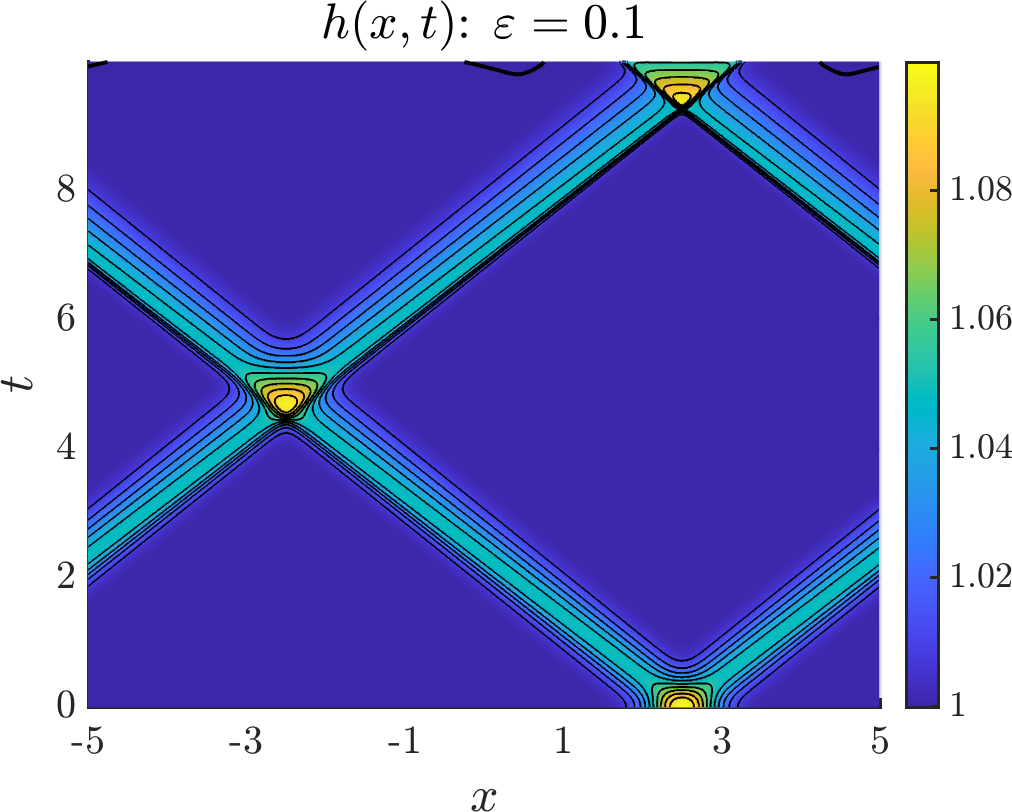
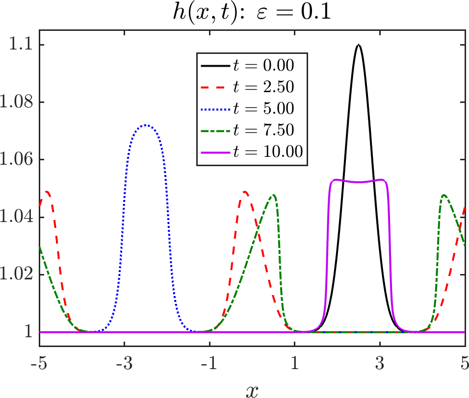
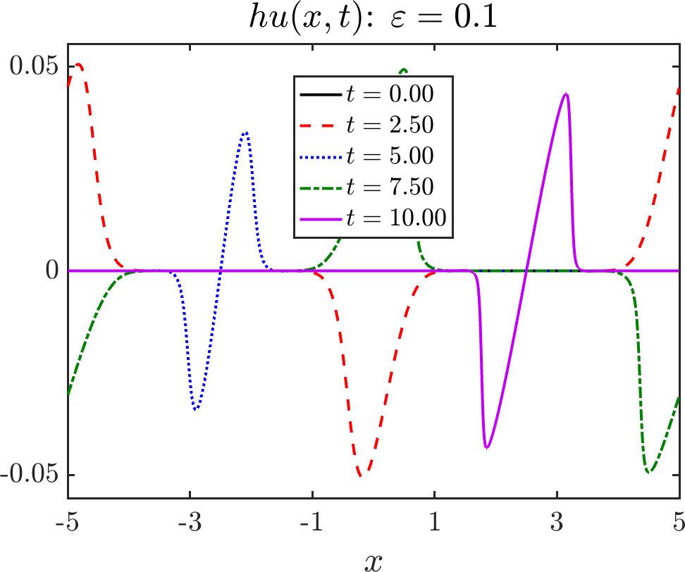
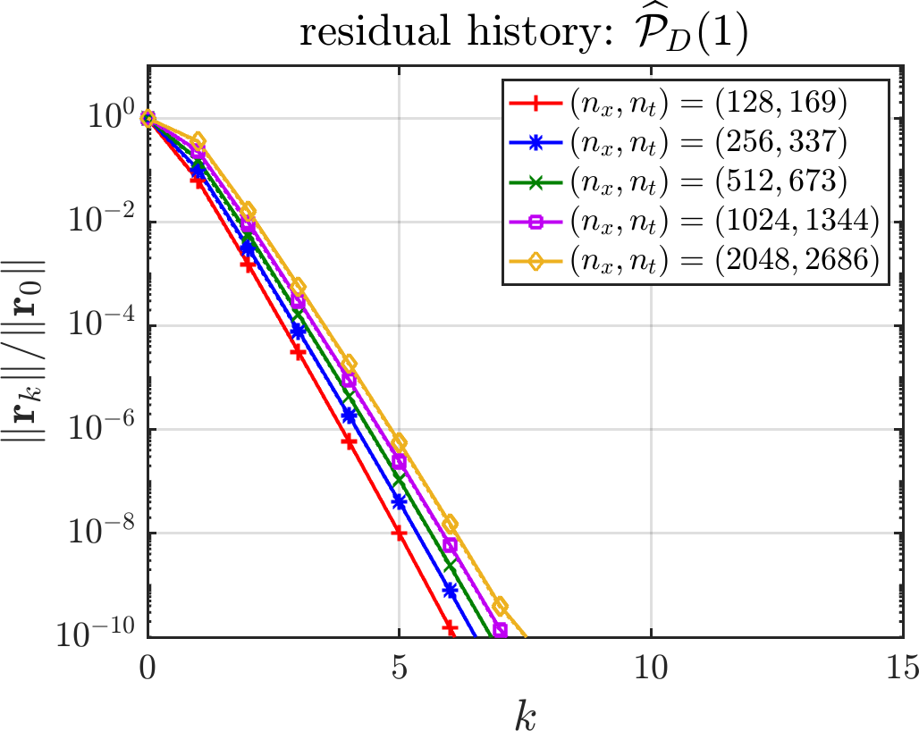
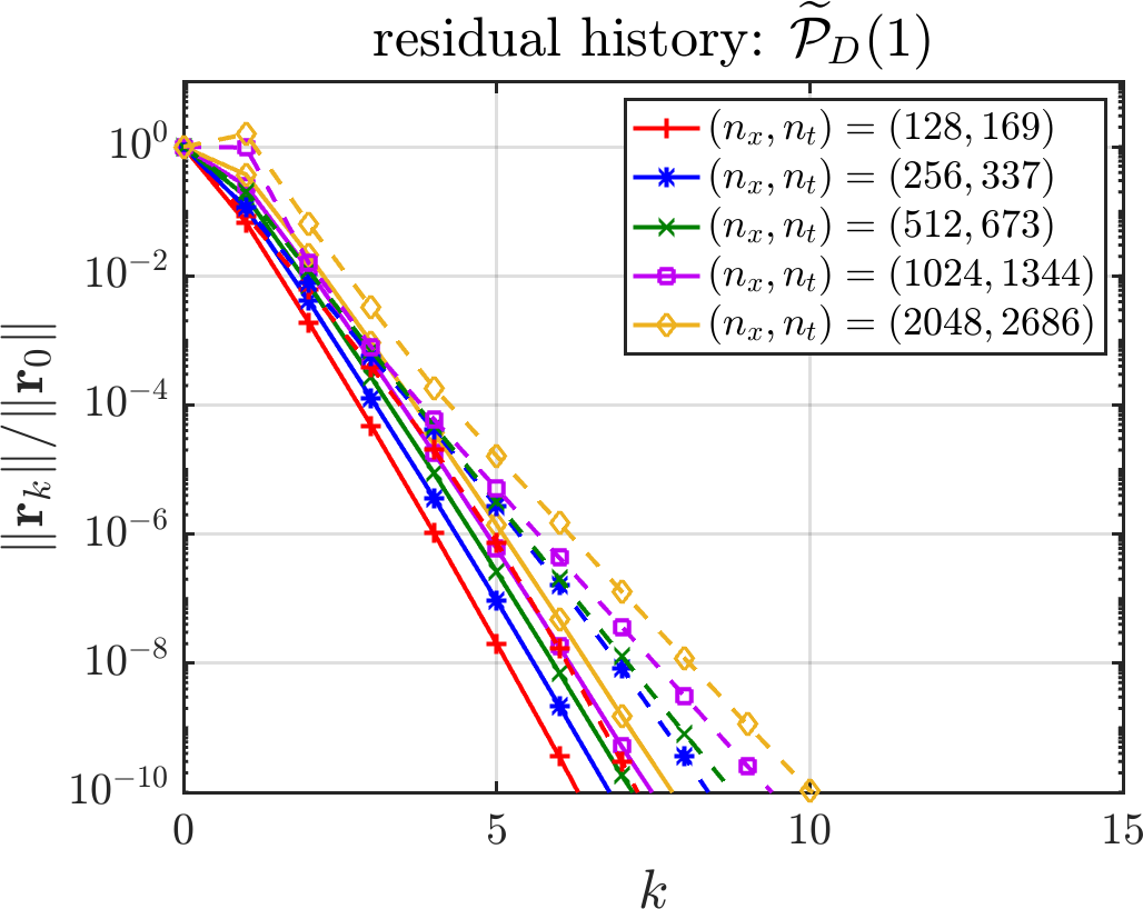
Figure 3: Small-amplitude (IDP) problem for (shallow-water), with $\varepsilon=0.1$. Bottom left: Nonlinear residual history with dotted lines corresponding to exact solves of the linearized problems ${\cal A}_{k}\bm{e}_{k}^{\rm lin}=\bm{r}_{k}$, and solid lines to approximate solves with a single iteration of Algorithm 1 using $\widehat{{\cal P}}$. Bottom right: Nonlinear residual history where linearized problems ${\cal A}_{k}\bm{e}_{k}^{\rm lin}=\bm{r}_{k}$ are approximately solved with a single iteration of Algorithm 1 using $\widetilde{{\cal P}}$ with diagonal blocks $\widetilde{{\cal A}}_{ii}$ either inverted exactly (solid lines) or approximately with one MGRIT V-cycle (dashed lines).

The results of the above problems are shown in Figs. 3, 4, 5, and 6 and the plots in each figure can be interpreted in the following way. Top row: Space-time contour of the first component of $\bm{q}$, and cross-sections at the times indicated for the first two components of $\bm{q}$. Bottom row: Nonlinear residual history using Algorithm 2 when linearized systems are solved directly with time-stepping, as in Line 2 of Algorithm 2, or approximately using inner-it applications of the characteristic-based preconditioned iteration Algorithm 1, as in Line 2 of Algorithm 2. Note that we do not show results for block triangular preconditioners $\widehat{\cal P}_{L}$ and $\widetilde{\cal P}_{L}$, since in all cases we find that their convergence behavior is essentially the same as that for the block diagonal preconditioners, $\widehat{\cal P}_{D}$, and $\widetilde{\cal P}_{D}$, respectively. Ideally inner-it $=1$, but results show more than one inner iteration is sometimes beneficial and even necessary for the outer iteration to converge. Recall that $\widehat{{\cal P}}$ uses diagonal blocks from $\widehat{\Phi}_{0}^{n}$ and $\widetilde{\cal P}$ uses a certain approximation to them. Plots in the bottom row of each figure include either $\widehat{{\cal P}}$(inner-it) or $\widehat{{\cal P}}$(inner-it) in their titles. Plots titled $\widehat{{\cal P}}$(inner-it) show results with linearized systems in Algorithm 2 either solved approximately with block preconditioner $\widehat{{\cal P}}$(inner-it) (solid lines), or solved exactly via time-stepping (dotted lines); note that all results using $\widehat{\cal P}$ apply the preconditioner exactly, i.e., using exact inverses for diagonal blocks $\widehat{{\cal A}}_{ii}$. Plots titled $\widetilde{\cal P}$(inner-it) show results for block preconditioning with $\widetilde{\cal P}$, with solid lines corresponding to exact inverses of diagonal blocks $\widetilde{{\cal A}}_{ii}$ and dashed lines to inexact inverses via one MGRIT V-cycle.

     

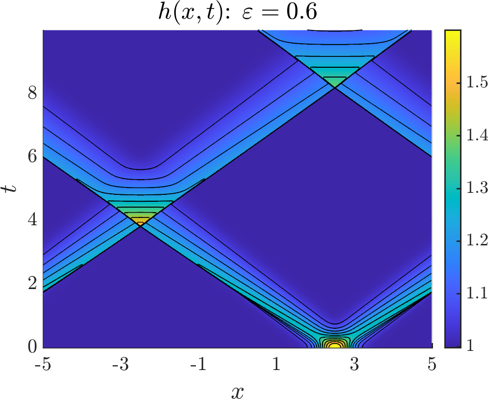
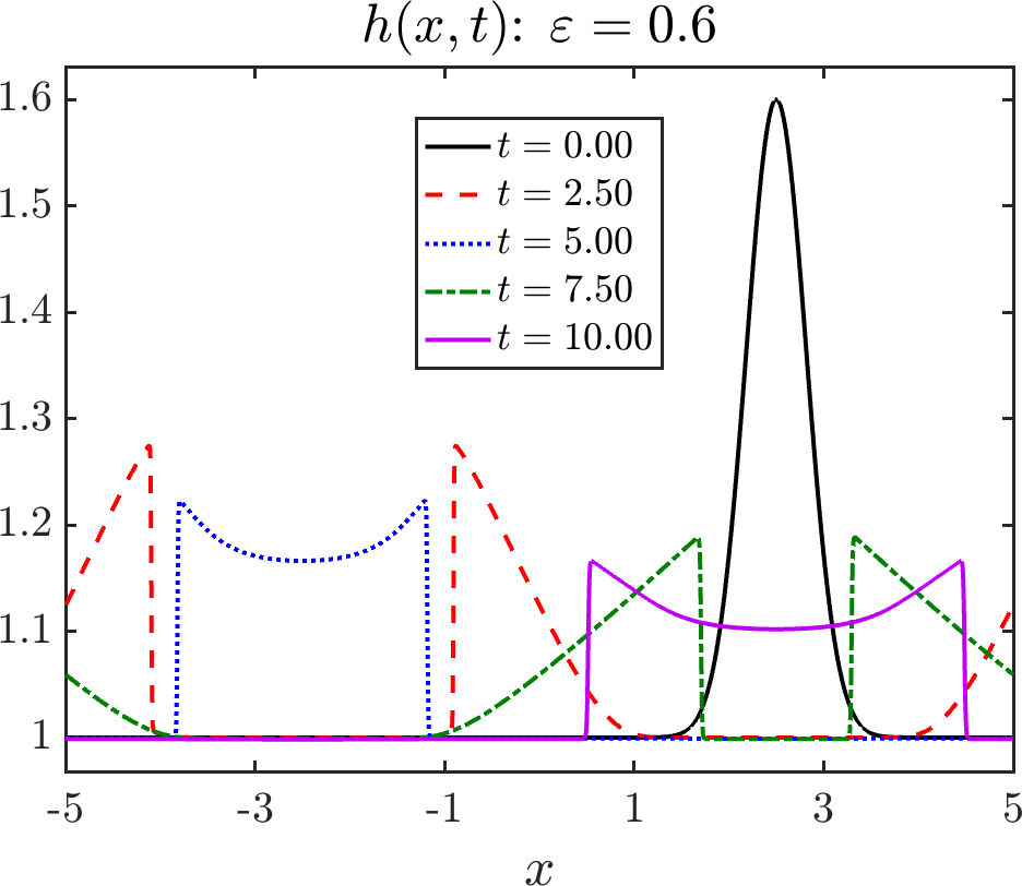
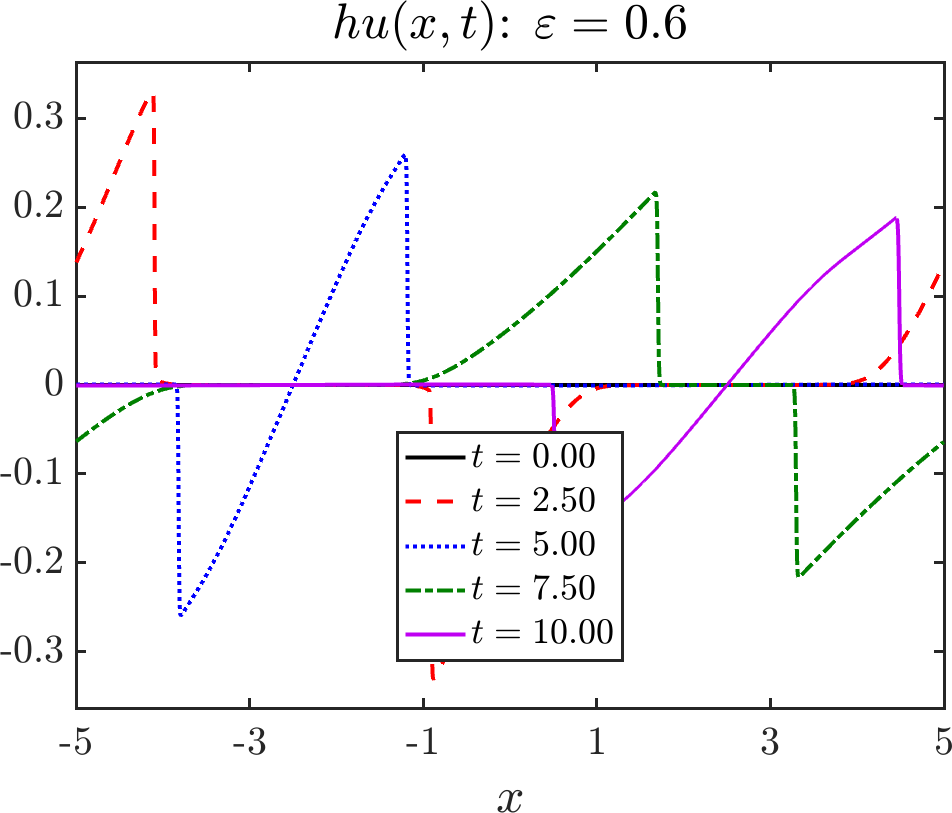
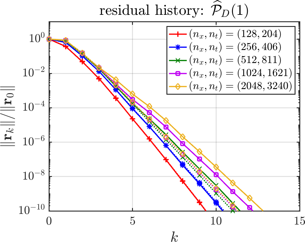
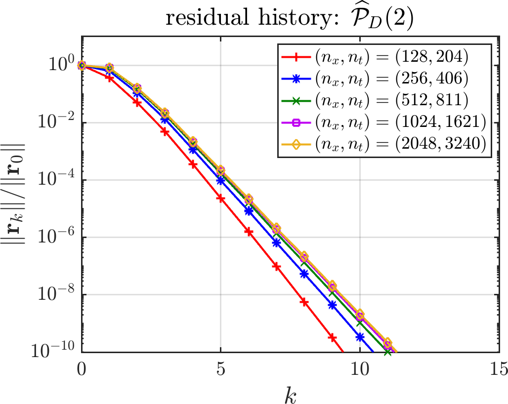
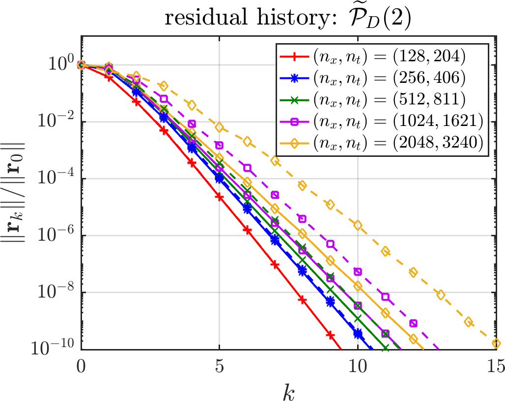
Figure 4: Larger-amplitude (IDP) problem for (shallow-water), with $\varepsilon=0.6$.

Some commentary is now in order. For all problems, when the linearized problems are solved directly, the solver quickly converges (i.e., the dotted lines in plots titled $\widehat{{\cal P}}$(inner-it), noting that these dotted lines often sit directly underneath the solid lines in these plots). This indicates that the idea of freezing the dissipation matrix in the linearization (35) is reasonable. This result also suggests that if one wishes to solve nonlinear hyperbolic systems parallel-in-time, then it suffices to know how to solve linear(ized) hyperbolic systems parallel-in-time. In all of the small-amplitude problems, the solver converges quickly, and there is essentially no deterioration in convergence when direct solves of linearized problems are replaced with a single iteration of either block preconditioner $\widehat{{\cal P}}$ or $\widetilde{{\cal P}}$. We also see little, if any, deterioration in convergence when diagonal blocks of $\widetilde{{\cal P}}$ are inverted inexactly via MGRIT—the dashed lines in plots titled $\widetilde{{\cal P}}$(inner-it).

     

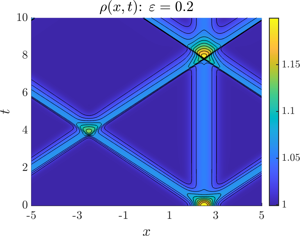
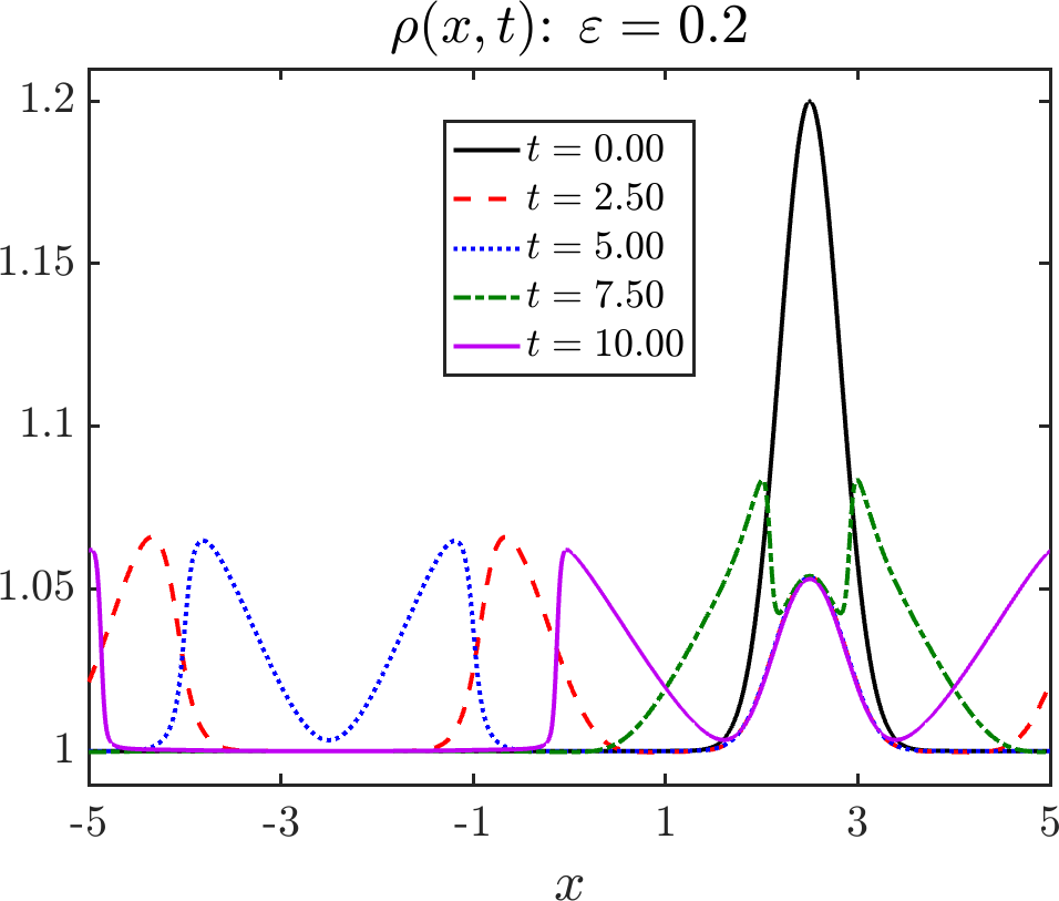
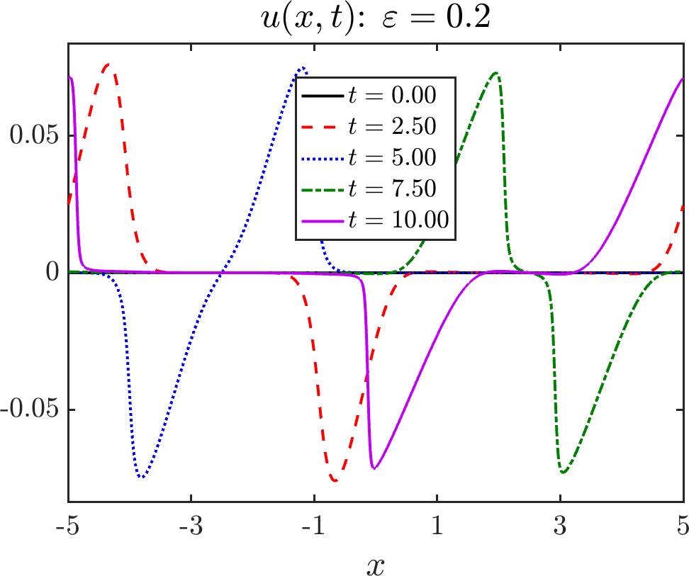
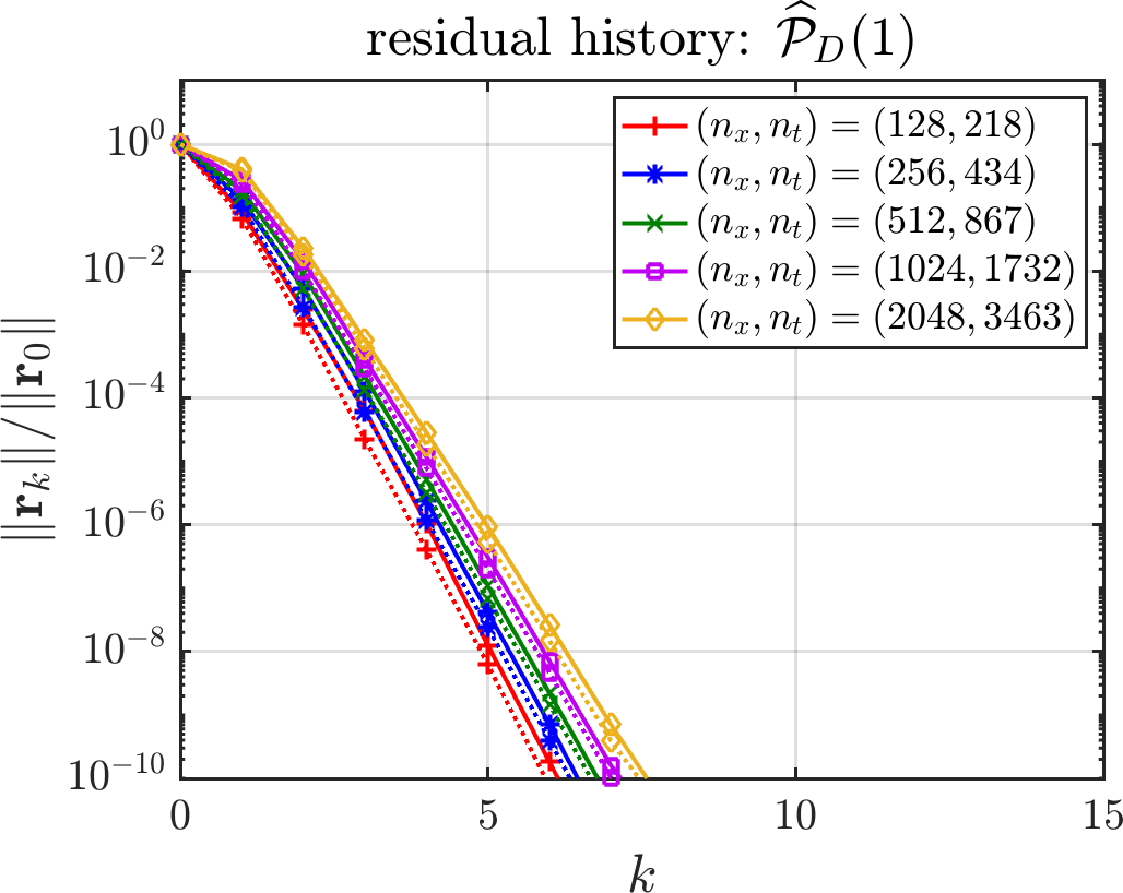
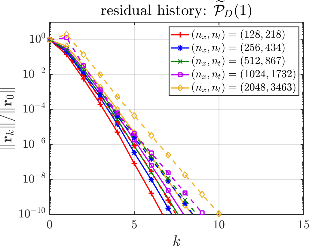
Figure 5: Small-amplitude (IDPP) problem for (euler) with $\varepsilon=0.2$.

     

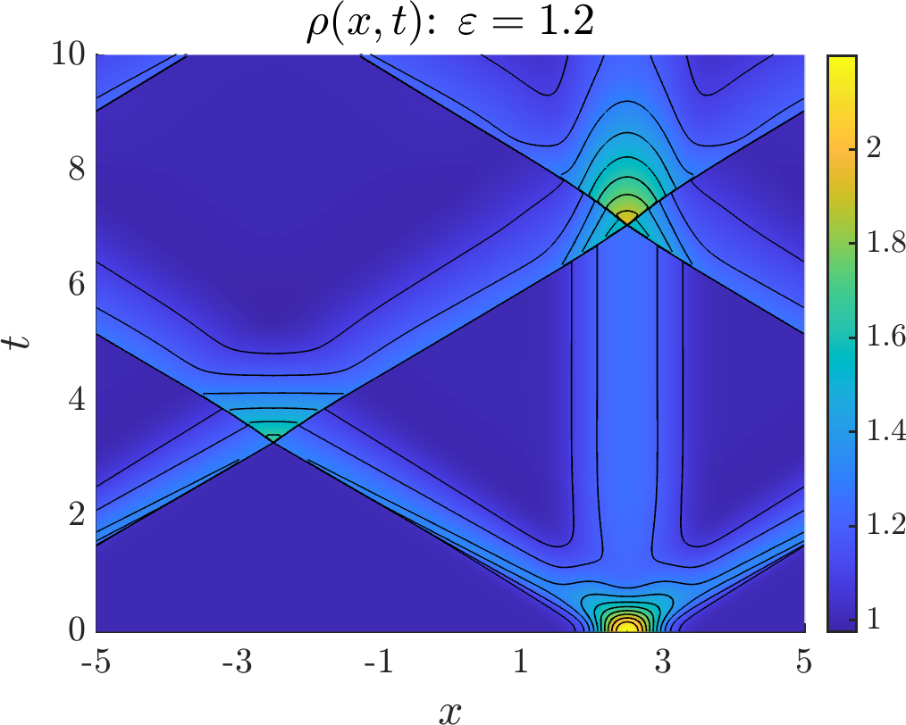
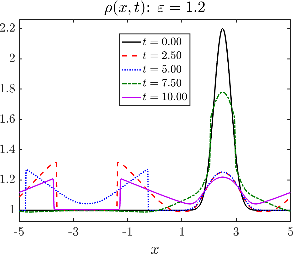
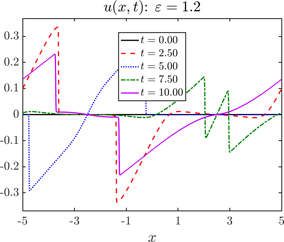
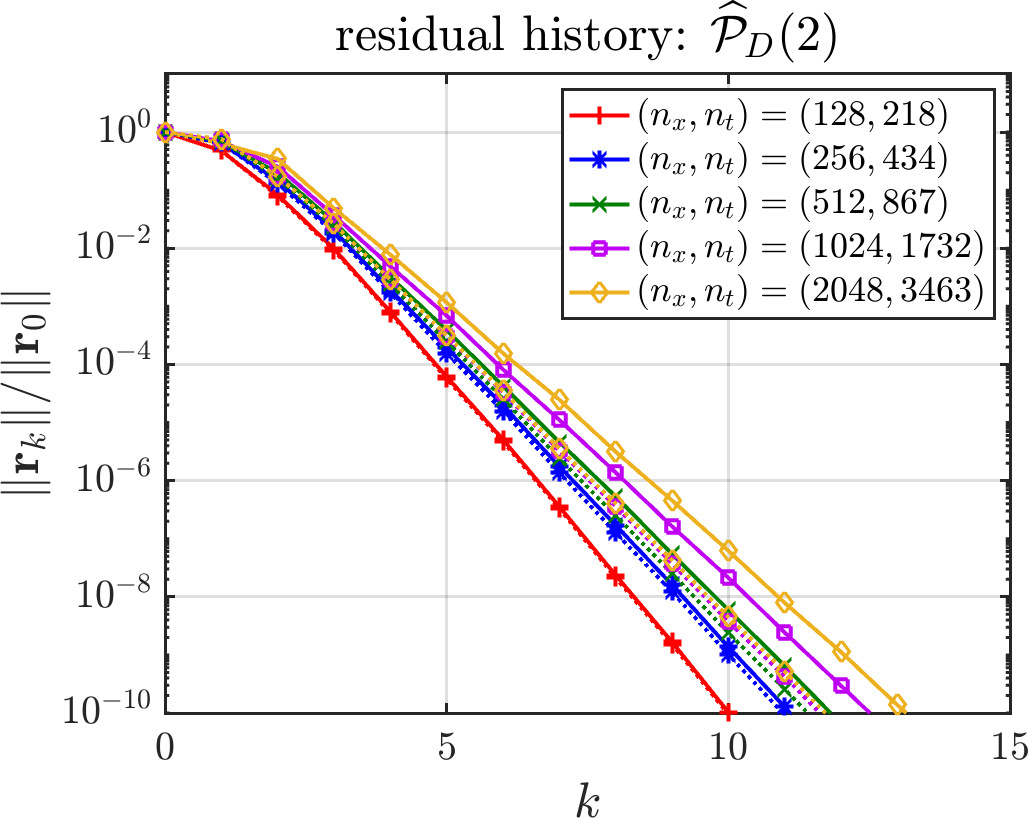
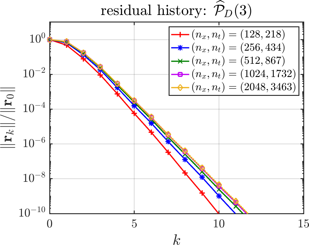
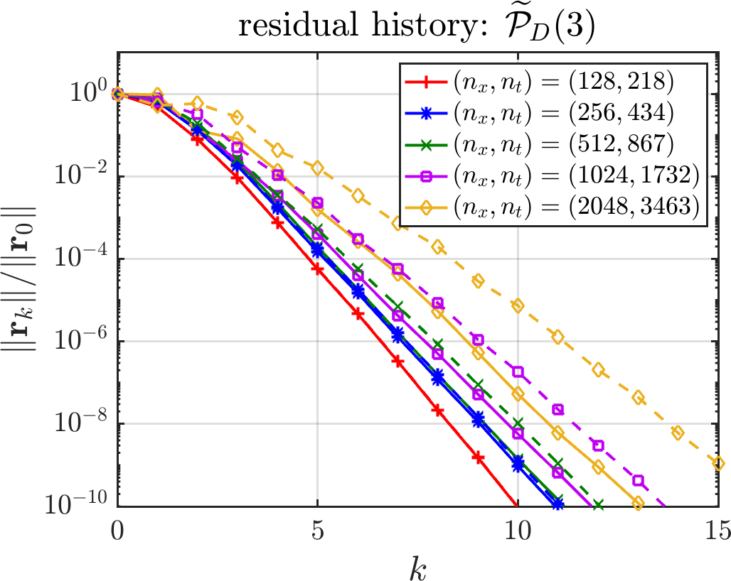
Figure 6: Larger-amplitude (IDPP) problem for (euler) with $\varepsilon=1.2$.

For the larger-amplitude problems, we see that, unsurprisingly, the number of iterations increases relative to the small-amplitude problems, but we emphasize that the solver still converges very quickly, at least when direct solves of linearized problems are used. When direct solves are replaced with block preconditioning, there is a slow degradation in convergence speed of the solver, with multiple inner iterations being required to restore scalability with respect to mesh size. In fact, in some cases the solver fails on sufficiently fine meshes if enough inner iterations are not used; for example, when $\widetilde{{\cal P}}$(1) is applied with exact inverses for $\widetilde{{\cal A}}_{ii}$ to the $(n_{x},n_{t})=(2048,3463)$ problem in Fig. 6, the solver produces a negative density. As a second example, even $\widetilde{{\cal P}}$(5) produced a negative density for the larger-amplitude Sod problem in Supplementary Materials Figure SM4 with $(n_{x},n_{t})=(2048,1348)$. Furthermore, in the larger-amplitude problems, there is often a large deterioration in performance when moving $\widehat{{\cal P}}$ to $\widetilde{{\cal P}}$. Thus, while these results represent an advancement in the area of parallel-in-time methods for nonlinear hyperbolic systems, and the number of outer iterations is still quite small for these difficult nonlinear problems, they indicate that further research is required to develop methods capable of solving nonlinear problems with strong shocks with iteration numbers that are fully mesh independent.

6 Conclusions and future outlook

We have presented a framework for the all-at-once solution of systems of hyperbolic PDEs in one spatial dimension, both linear and nonlinear, that can admit parallelism in time. The crux of the approach is a block preconditioner applied in the characteristic-variables associated with the linear(ized) PDE. Transforming to characteristic variables is motivated by the observation that inter-variable coupling is generally weaker than in the original variables. For an $\ell$-dimensional PDE system, application of the preconditioner requires solving $\ell$ scalar linear-advection-like PDEs, which can, at least in principle, be approximated parallel-in-time. While we considered only serial implementations, the small number of MGRIT iterations required in our acoustics and small-amplitude nonlinear tests is consistent with obtaining parallel speed-ups over sequential time-stepping [11, 13].

In essence, the effectiveness of our approach boils down to the approximation of a block lower triangular space-time Schur complement. In a certain sense, the complexity of this Schur complement relates to the coupling strength between characteristic variables in the linear(ized) PDE. Our current approach deteriorates with increasingly strong spatio-temporal variation in the eigenvectors of the flux Jacobian, e.g., when transitioning from a problem with weak shocks to one with stronger shocks. In future work we hope to improve the robustness of our solver against such variations. Higher-order discretizations could also be considered, which for acoustics in heterogeneous media are often nonlinear due to limiters [19], and for systems of nonlinear conservation laws there is potential based on our previous success with high-order WENO discretizations of scalar conservation laws [12]. Other directions include multiple spatial dimensions, parallel implementations, and the application of these ideas to advection-diffusion PDE systems like the Navier–Stokes equations.

Appendix A Proof of Lemma 3.1

Proof A.1.

We begin by computing the triple-matrix product $\widehat{\Phi}:={\cal R}_{0}^{-1}\Phi{\cal R}_{0}$, where

(47) $${\cal R}_{0}^{-1}=\frac{1}{2}\begin{bmatrix}-{\cal Z}_{0}^{-1}&I\\ {\cal Z}_{0}^{-1}&I\end{bmatrix},\quad\Phi=\begin{bmatrix}\Phi_{pp}&\Phi_{pu}\\ \Phi_{up}&\Phi_{uu}\end{bmatrix},\quad{\cal R}_{0}=\begin{bmatrix}-{\cal Z}_{0}&{\cal Z}_{0}\\ I&I\end{bmatrix}.$$

Multiplying this out gives

(48a) $$\widehat{\Phi}_{22} =\tfrac{1}{2}\Big{[}\big{(}\Phi_{uu}+{\cal Z}_{0}^{-1}\Phi_{pp}{\cal Z}_{0}\big{)}+\big{(}\Phi_{up}{\cal Z}_{0}+{\cal Z}_{0}^{-1}\Phi_{pu}\big{)}\Big{]},$$

(48b) $$\widehat{\Phi}_{11} =\tfrac{1}{2}\Big{[}\big{(}\Phi_{uu}+{\cal Z}_{0}^{-1}\Phi_{pp}{\cal Z}_{0}\big{)}-\big{(}\Phi_{up}{\cal Z}_{0}+{\cal Z}_{0}^{-1}\Phi_{pu}\big{)}\Big{]},$$

(48c) $$\widehat{\Phi}_{12} =\tfrac{1}{2}\Big{[}\big{(}\Phi_{uu}-{\cal Z}_{0}^{-1}\Phi_{pp}{\cal Z}_{0}\big{)}+\big{(}\Phi_{up}{\cal Z}_{0}-{\cal Z}_{0}^{-1}\Phi_{pu}\big{)}\Big{]},$$

(48d) $$\widehat{\Phi}_{21} =\tfrac{1}{2}\Big{[}\big{(}\Phi_{uu}-{\cal Z}_{0}^{-1}\Phi_{pp}{\cal Z}_{0}\big{)}-\big{(}\Phi_{up}{\cal Z}_{0}-{\cal Z}_{0}^{-1}\Phi_{pu}\big{)}\Big{]}.$$

Notice that the same four matrices appear in each of the four blocks here, i.e., those inside the open parentheses. Plugging in the form of the blocks of $\Phi$ from (7) and using the fact that ${\cal C}_{0}$ and ${\cal Z}_{0}^{-1}$ commute due to their both being diagonal gives

(49a) $$\widehat{\Phi}_{22} =I -\frac{\delta t}{2h}{\cal C}_{0}\Big{[}\big{(}{\cal L}_{uu}+{\cal Z}_{0}^{-1}{\cal L}_{pp}{\cal Z}_{0}\big{)}+\big{(}{\cal L}_{up}{\cal Z}_{0}+{\cal Z}_{0}^{-1}{\cal L}_{pu}\big{)}\Big{]},$$

(49b) $$\widehat{\Phi}_{11} =I -\frac{\delta t}{2h}{\cal C}_{0}\Big{[}\big{(}{\cal L}_{uu}+{\cal Z}_{0}^{-1}{\cal L}_{pp}{\cal Z}_{0}\big{)}-\big{(}{\cal L}_{up}{\cal Z}_{0}+{\cal Z}_{0}^{-1}{\cal L}_{pu}\big{)}\Big{]},$$

(49c) $$\widehat{\Phi}_{12} = -\frac{\delta t}{2h}{\cal C}_{0}\Big{[}\big{(}{\cal L}_{uu}-{\cal Z}_{0}^{-1}{\cal L}_{pp}{\cal Z}_{0}\big{)}+\big{(}{\cal L}_{up}{\cal Z}_{0}-{\cal Z}_{0}^{-1}{\cal L}_{pu}\big{)}\Big{]},$$

(49d) $$\widehat{\Phi}_{21} = -\frac{\delta t}{2h}{\cal C}_{0}\Big{[}\big{(}{\cal L}_{uu}-{\cal Z}_{0}^{-1}{\cal L}_{pp}{\cal Z}_{0}\big{)}-\big{(}{\cal L}_{up}{\cal Z}_{0}-{\cal Z}_{0}^{-1}{\cal L}_{pu}\big{)}\Big{]}.$$

Now we compute ${\cal Z}_{0}^{-1}{\cal L}_{pp}{\cal Z}_{0}$, ${\cal Z}_{0}^{-1}{\cal L}_{pu}$, ${\cal L}_{up}{\cal Z}_{0}$, and ${\cal L}_{uu}$, with stencils for ${\cal L}_{ij}$ in (8). Since ${\cal Z}_{0}^{-1}$ is a diagonal matrix, left-multiplying a matrix by it scales the rows of that matrix by its diagonal entries, while right-multiplying a matrix by ${\cal Z}_{0}$ scales the columns of that matrix by the diagonal entries of ${\cal Z}_{0}$. Thus,

(50a) $$\big{[}{\cal Z}_{0}^{-1}{\cal L}_{pp}{\cal Z}_{0}\big{]}_{i} =\left[-\frac{Z_{i-1}}{Z_{i-1}+Z_{i}},\,\frac{Z_{i}}{Z_{i-1}+Z_{i}}+\frac{Z_{i}}{Z_{i}+Z_{i+1}},\,-\frac{Z_{i+1}}{Z_{i}+Z_{i+1}}\right],$$

(50b) $$\big{[}{\cal Z}_{0}^{-1}{\cal L}_{pu}\big{]}_{i} =\left[-\frac{Z_{i-1}}{Z_{i-1}+Z_{i}},\,\frac{Z_{i-1}}{Z_{i-1}+Z_{i}}-\frac{Z_{i+1}}{Z_{i}+Z_{i+1}},\,\frac{Z_{i+1}}{Z_{i}+Z_{i+1}}\right],$$

(50c) $$\big{[}{\cal L}_{up}{\cal Z}_{0}\big{]}_{i} =\left[-\frac{Z_{i-1}}{Z_{i-1}+Z_{i}},\,\frac{Z_{i}}{Z_{i-1}+Z_{i}}-\frac{Z_{i}}{Z_{i}+Z_{i+1}},\,\frac{Z_{i+1}}{Z_{i}+Z_{i+1}}\right],$$

(50d) $$\big{[}{\cal L}_{uu}\big{]}_{i} =\left[-\frac{Z_{i-1}}{Z_{i-1}+Z_{i}},\,\frac{Z_{i-1}}{Z_{i-1}+Z_{i}}+\frac{Z_{i+1}}{Z_{i}+Z_{i+1}},\,-\frac{Z_{i+1}}{Z_{i}+Z_{i+1}}\right].$$

Using the above expressions, we now compute the stencils of the terms in (49):

(51a) $$\big{[}{\cal L}_{uu}+{\cal Z}_{0}^{-1}{\cal L}_{pp}{\cal Z}_{0}\big{]}_{i} =\left[-\frac{2Z_{i-1}}{Z_{i-1}+Z_{i}},\,2,\,-\frac{2Z_{i+1}}{Z_{i}+Z_{i+1}}\right],$$

(51b) $$\big{[}{\cal L}_{uu}-{\cal Z}_{0}^{-1}{\cal L}_{pp}{\cal Z}_{0}\big{]}_{i} =\left[0,\,\frac{Z_{i-1}-Z_{i}}{Z_{i-1}+Z_{i}}-\frac{Z_{i}-Z_{i+1}}{Z_{i}+Z_{i+1}},\,0\right],$$

(51c) $$\big{[}{\cal L}_{up}{\cal Z}_{0}+{\cal Z}_{0}^{-1}{\cal L}_{pu}\big{]}_{i} =\left[-\frac{2Z_{i-1}}{Z_{i-1}+Z_{i}},\,0,\,\frac{2Z_{i+1}}{Z_{i}+Z_{i+1}}\right],$$

(51d) $$\big{[}{\cal L}_{up}{\cal Z}_{0}-{\cal Z}_{0}^{-1}{\cal L}_{pu}\big{]}_{i} =\left[0,\,-\frac{Z_{i-1}-Z_{i}}{Z_{i-1}+Z_{i}}-\frac{Z_{i}-Z_{i+1}}{Z_{i}+Z_{i+1}},\,0\right].$$

Plugging these expressions into (49) and simplifying concludes the proof.

SUPPLEMENTARY MATERIALS: PinT solution of hyperbolic systemsH. De Sterck, R. D. Falgout, O. A. Krzysik, J. B. Schroder

SUPPLEMENTARY MATERIALS: PARALLEL-IN-TIME SOLUTION OF HYPERBOLIC PDE SYSTEMS VIA CHARACTERISTIC-VARIABLE BLOCK PRECONDITIONING

Appendix SM1 Flux Jacobians and their eigen decompositions

The flux Jacobian of (shallow-water) is

(SM1) $$f^{\prime}(\bm{q})=\begin{bmatrix}0&1\\ -u^{2}+h&2u\end{bmatrix}.$$

The eigenvalues of this matrix are $\lambda^{1}=u-\sqrt{h}$ and $\lambda^{2}=u+\sqrt{h}$, with corresponding right and left eigenvector matrices given by

(SM2) $$R=\begin{bmatrix}1&1\\ \lambda^{1}&\lambda^{2}\end{bmatrix},\quad R^{-1}=\frac{1}{\lambda^{2}-\lambda^{1}}\begin{bmatrix}\lambda^{2}&-1\\ -\lambda^{1}&1\end{bmatrix},$$

respectively. The flux Jacobian of (euler) is

(SM3) $$f^{\prime}(\bm{q})=\begin{bmatrix}0&1&0\\ \tfrac{1}{2}(\gamma-3)u^{2}&(3-\gamma)u&\gamma-1\\ \tfrac{1}{2}(\gamma-1)u^{3}-uH&H-(\gamma-1)u^{2}&\gamma u\end{bmatrix},$$

where $H=\frac{E+p}{\rho}$ is the total specific enthalpy, and $c=\sqrt{\frac{\gamma p}{\rho}}$ is the sound speed. The eigenvalues are $\lambda^{1}=u-c$, $\lambda^{2}=u$, and $\lambda^{3}=u+c$, with the associated right and left eigenvector matrices given by

(SM4) $$R=\begin{bmatrix}1&1&1\\ u-c&u&u+c\\ H-uc&\tfrac{1}{2}u^{2}&H+uc\end{bmatrix},\quad R^{-1}=\tfrac{\gamma-1}{2c^{2}}\begin{bmatrix}H+\tfrac{c(u-c)}{\gamma-1}&-u-\tfrac{c}{\gamma-1}&1\\ \tfrac{4c^{2}}{\gamma-1}-2H&2u&-2\\ H-\tfrac{c(u+c)}{\gamma-1}&-u+\tfrac{c}{\gamma-1}&1\end{bmatrix},$$

respectively.

Appendix SM2 Additional numerical results for nonlinear problems

Here we consider additional numerical results to complement those already in Section 5.4. In particular we consider standard Riemann problems. The layout of the plots in the figures below is the same as in Section 5.4, with the exception that residual histories with $\widetilde{\cal P}$(inner-it) in the title no longer include dashed lines corresponding to inexact inverses of $\widetilde{{\cal A}}_{ii}$ via MGRIT.

The two problems we consider are as follows. First, consider (shallow-water) for the dam break problem:

(DB) $$h(x,0) =\begin{cases}1+\varepsilon,\quad&x<0\\ 1\quad&x\geq 0,\end{cases}\quad u(x,0)=0,$$

with $(x,t)\in(-10,10)\times(0,5)$, $c_{0}=0.8$, and with constant boundary conditions. Small- and larger-amplitude results are shown in Figs. SM1 and SM2, respectively. Second, consider the following Sod problem for (euler):

(Sod) $$\rho(x,0)=\begin{cases}1,\quad&x<0.5\\ 1-\varepsilon,\quad&x\geq 0.5\end{cases},\quad u(x,0)=0,\quad E(x,0)=\frac{\rho(x,0)}{\gamma-1},$$

with $(x,t)\in(0,1)\times(0,0.25)$, $c_{0}=0.45$, and with constant boundary conditions. Small- and larger-amplitude results are shown in Figs. SM3 and SM4, respectively.

     

  

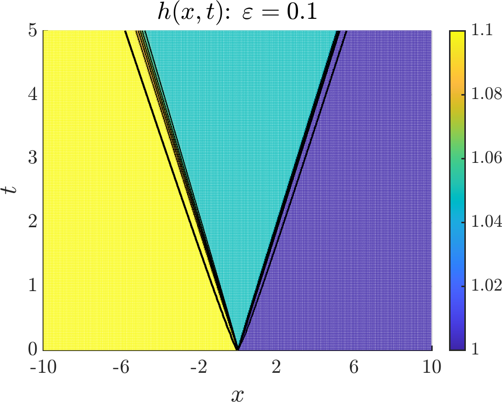
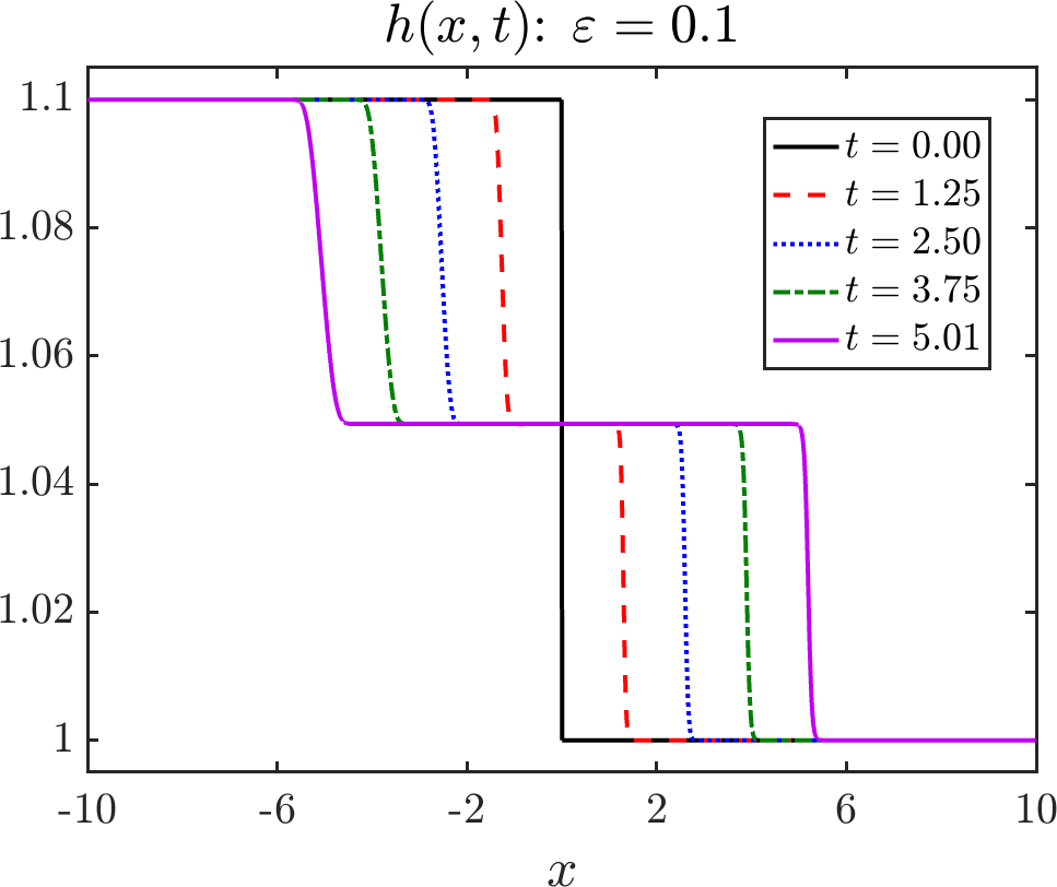
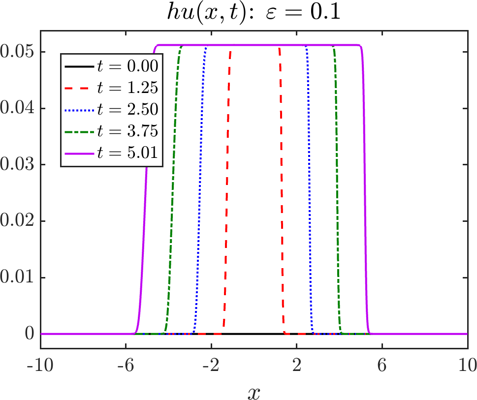
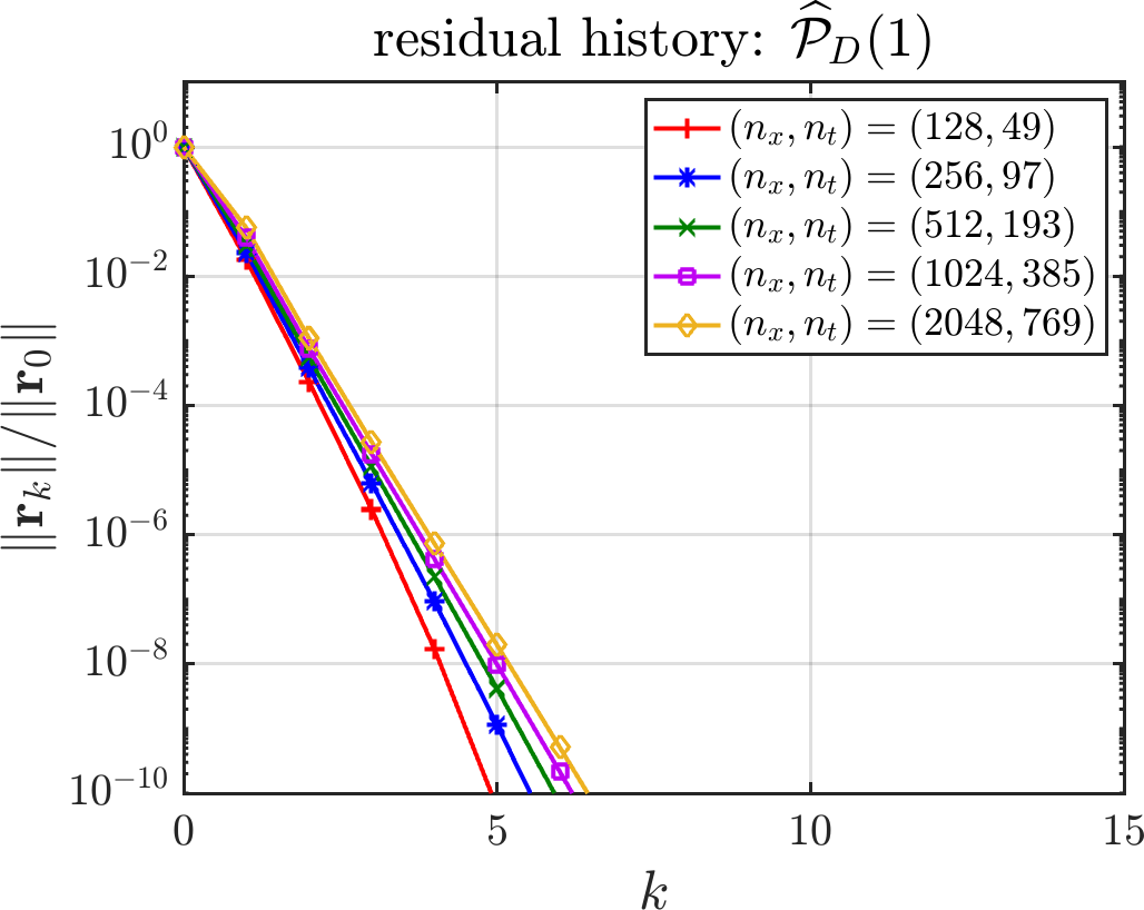
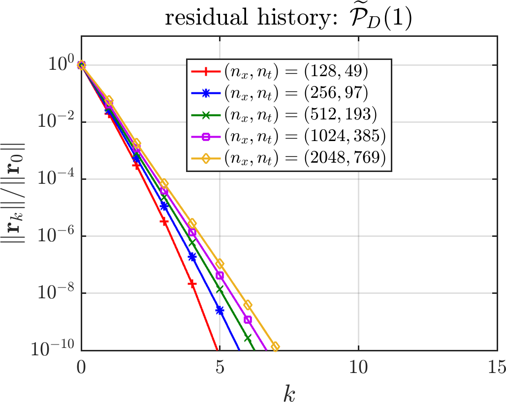
Figure SM1: Small-amplitude dam break problem (DB) for (shallow-water), with $\varepsilon=0.1$.

     

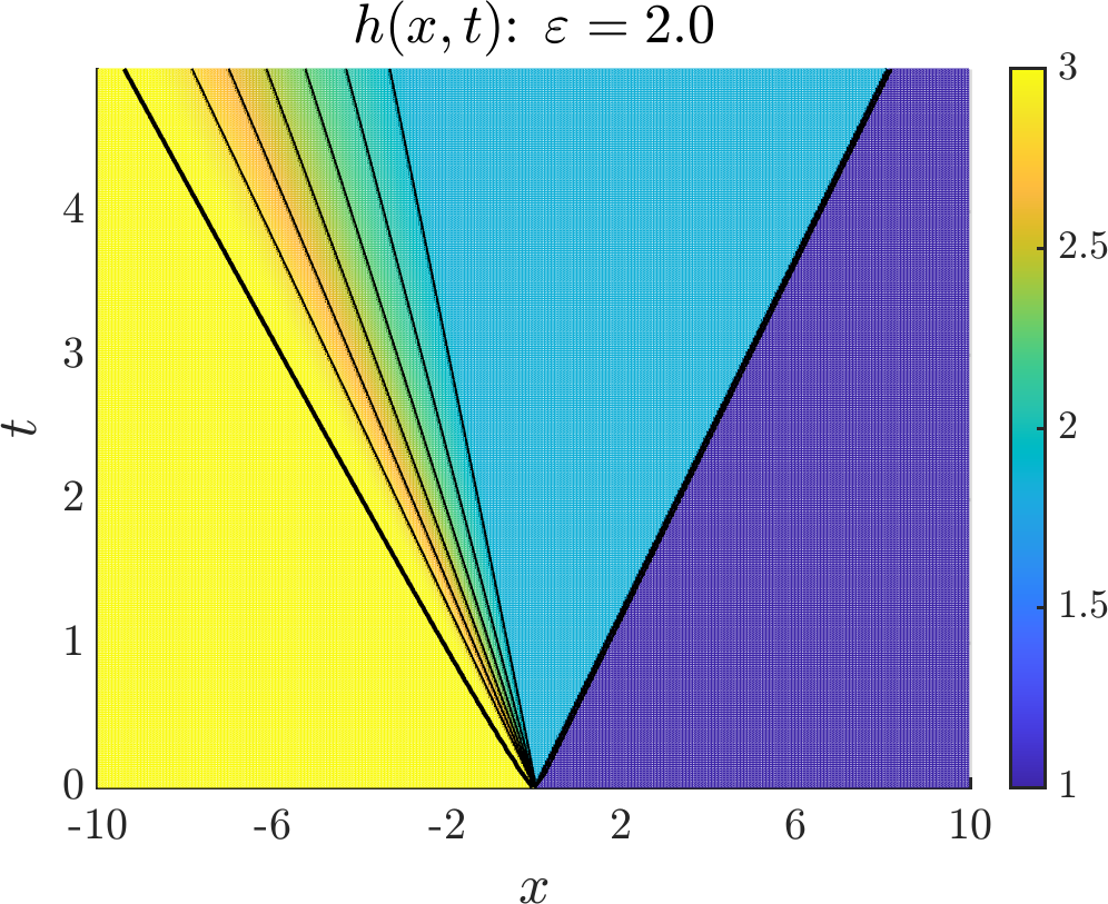
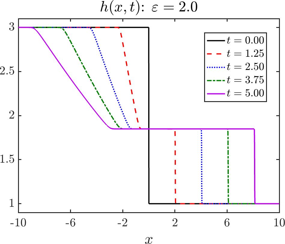
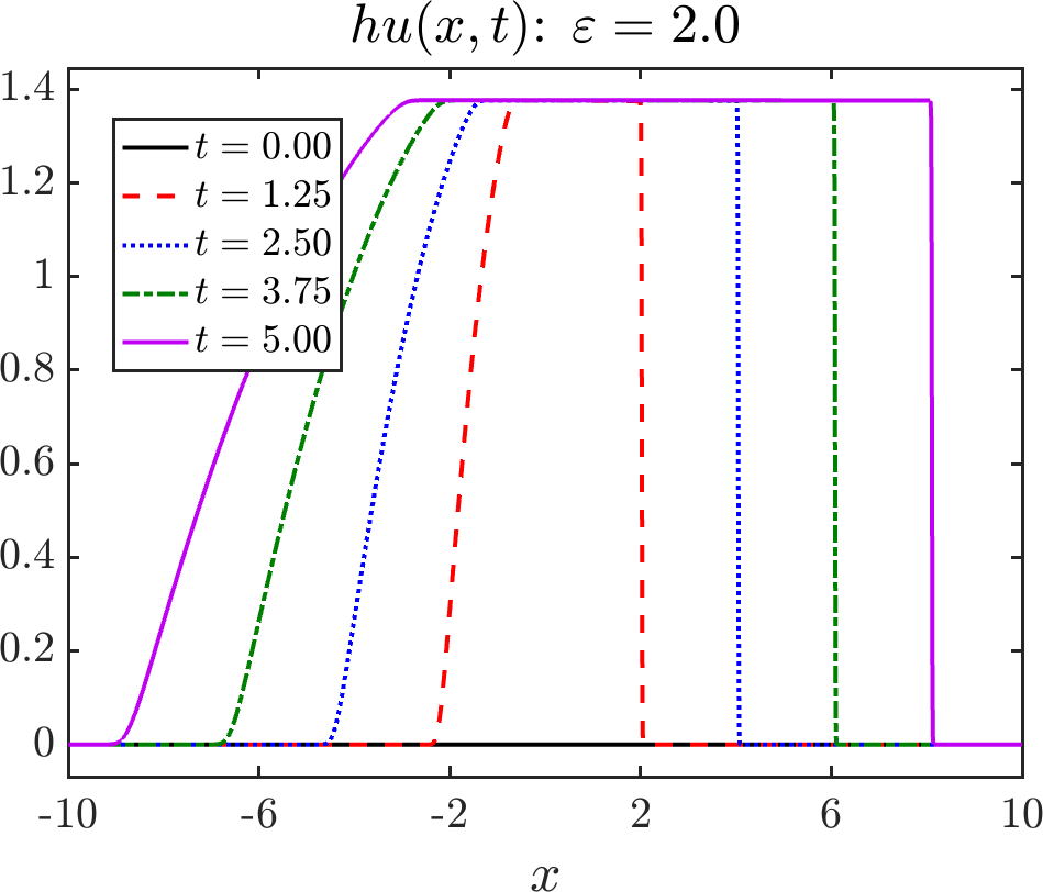
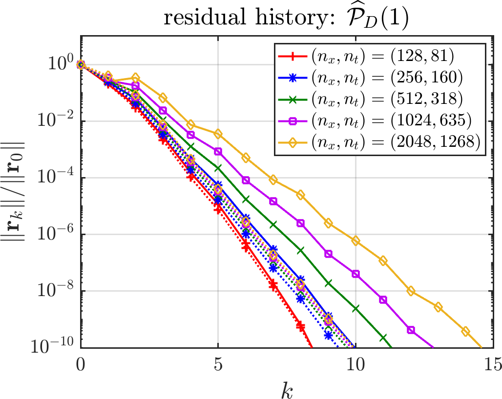
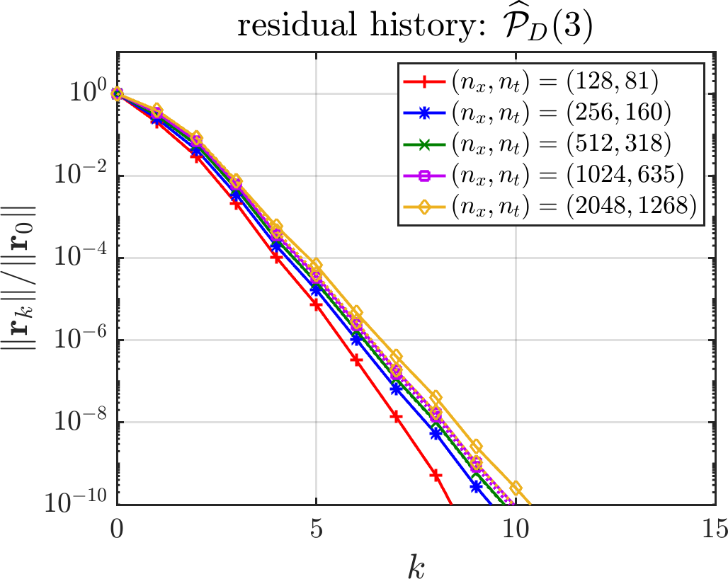
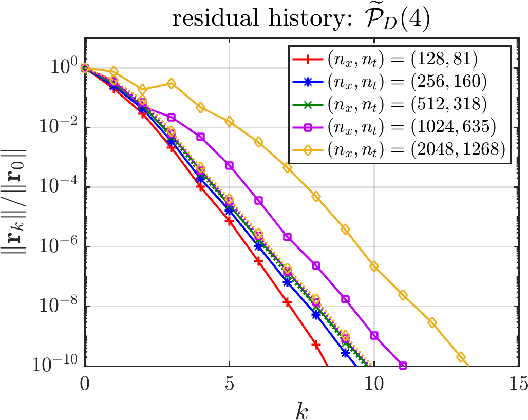
Figure SM2: Larger-amplitude dam break problem (DB) for (shallow-water), with $\varepsilon=2.0$. Dotted lines in plots with $\widehat{{\cal P}}$ in their titles correspond to exact solution of linearized systems.

     

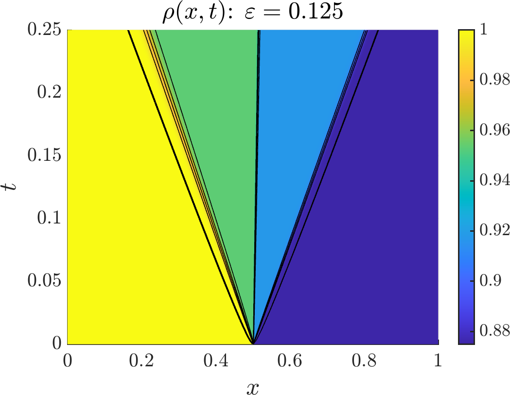
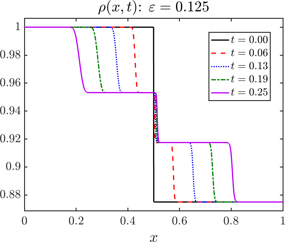
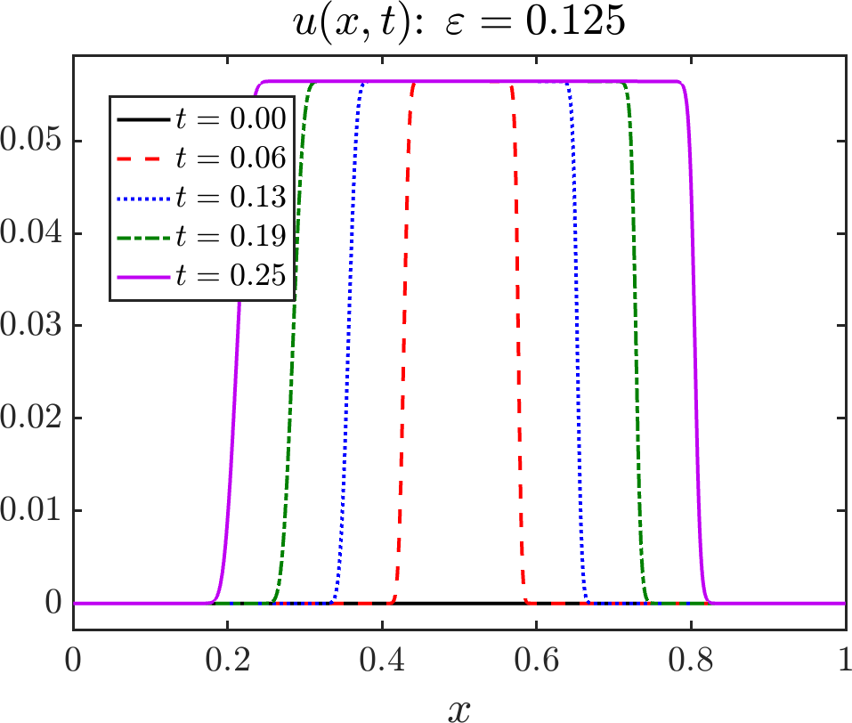
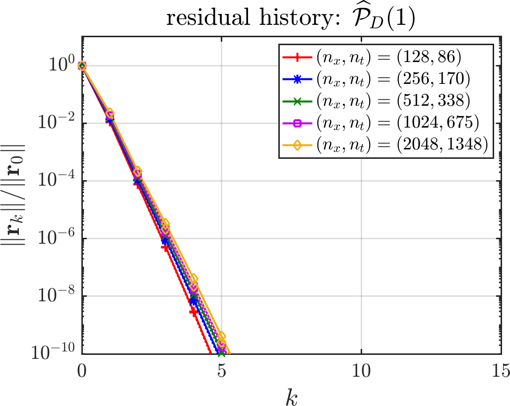
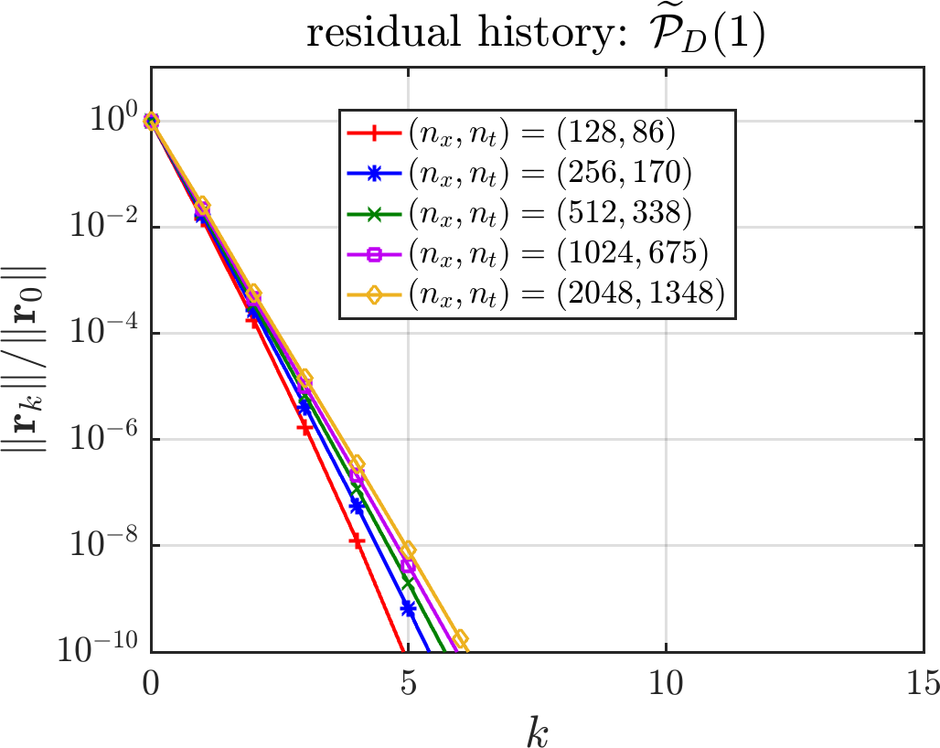
Figure SM3: Small-amplitude Sod problem (Sod) for (euler) with $\varepsilon=0.125$.

     

  

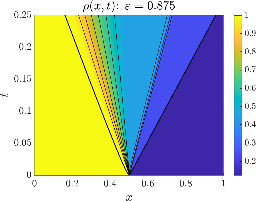
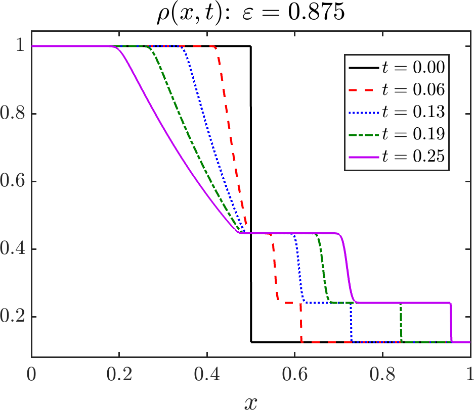
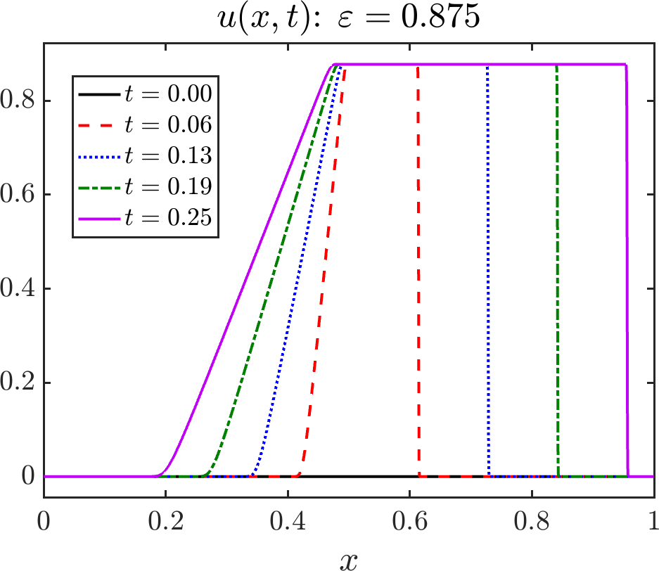
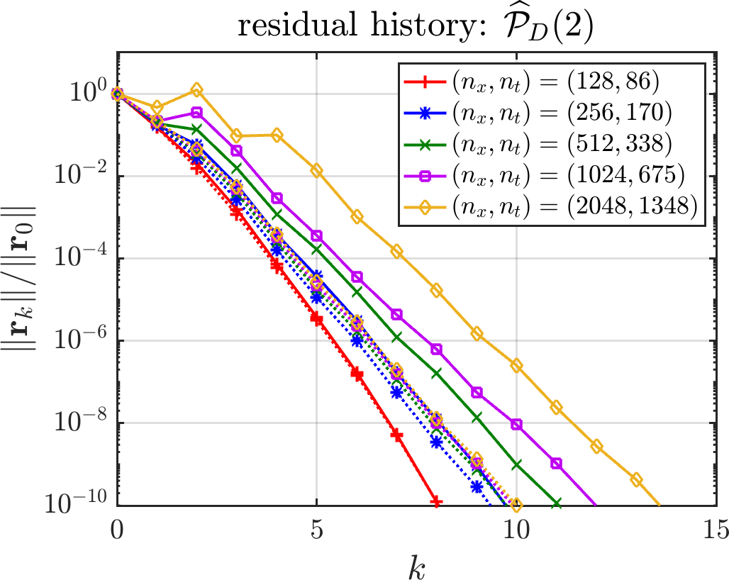
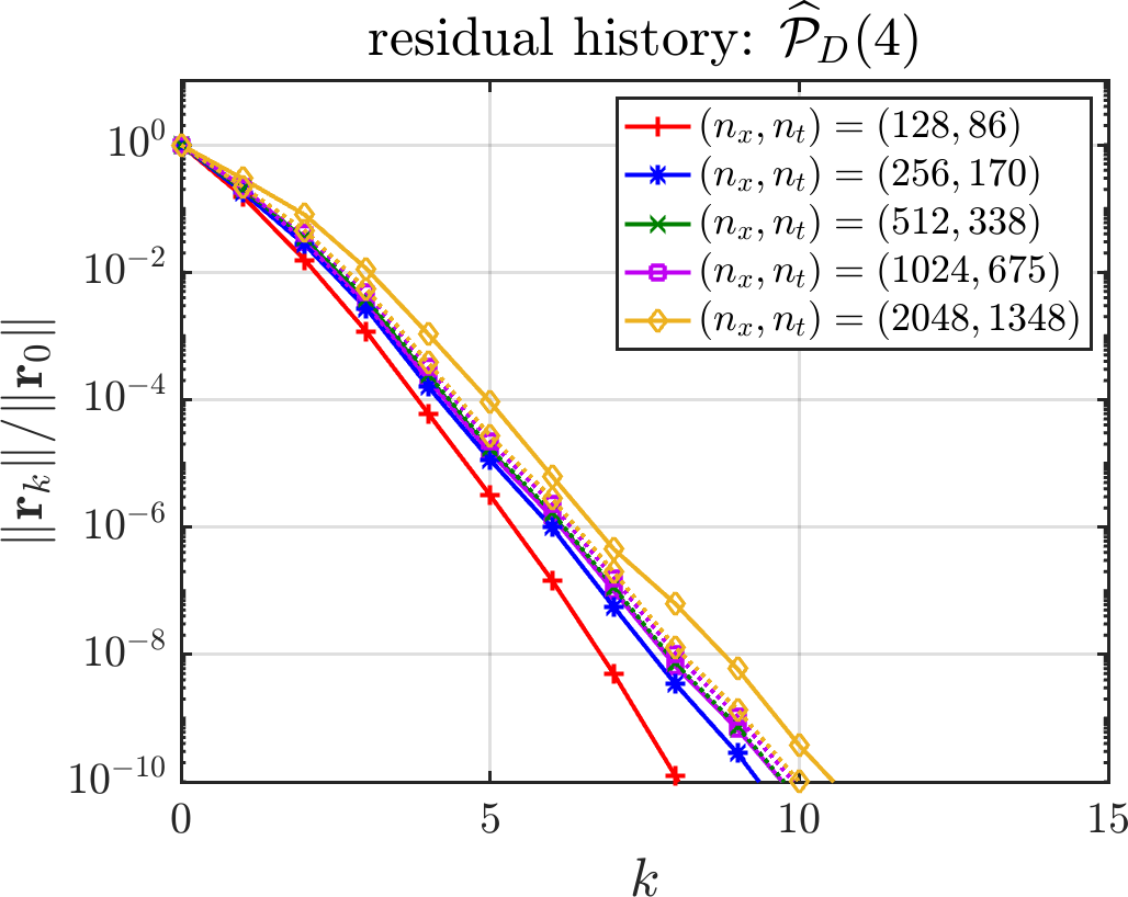
Figure SM4: Larger-amplitude Sod problem (Sod) for (euler) with $\varepsilon=0.875$.

References

- [1] D. S. Bale, R. J. LeVeque, S. Mitran, and J. A. Rossmanith, A wave propagation method for conservation laws and balance laws with spatially varying flux functions, SIAM J. Sci. Comput., 24 (2003), pp. 955–978.
- [2] J. G. Caldas Steinstraesser, P. d. S. Peixoto, and M. Schreiber, Parallel-in-time integration of the shallow water equations on the rotating sphere using Parareal and MGRIT, J. Comput. Phys., 496 (2024), p. 112591.
- [3] J. Christopher, R. D. Falgout, J. B. Schroder, S. M. Guzik, and X. Gao, A space-time parallel algorithm with adaptive mesh refinement for computational fluid dynamics, Comput. Vis. Sci., 23 (2020).
- [4] C. M. Dafermos, Hyperbolic Conservation Laws in Continuum Physics, Springer Berlin Heidelberg, 2010.
- [5] X. Dai and Y. Maday, Stable Parareal in time method for first-and second-order hyperbolic systems, SIAM J. Sci. Comput., 35 (2013), pp. A52–A78.
- [6] F. Danieli and S. MacLachlan, Multigrid reduction in time for non-linear hyperbolic equations, Electron. Trans. Numer. Anal., 58 (2023), pp. 43–65.
- [7] F. Danieli, B. S. Southworth, and J. B. Schroder, Space-time block preconditioning for incompressible resistive magnetohydrodynamics, (2023), https://arxiv.org/abs/2309.00768.
- [8] F. Danieli, B. S. Southworth, and A. J. Wathen, Space-time block preconditioning for incompressible flow, SIAM J. Sci. Comput., 44 (2022), p. A337–A363.
- [9] F. Danieli and A. J. Wathen, All-at-once solution of linear wave equations, Numer. Linear Algebra Appl., 28 (2021).
- [10] H. De Sterck, R. D. Falgout, S. Friedhoff, O. A. Krzysik, and S. P. MacLachlan, Optimizing multigrid reduction-in-time and Parareal coarse-grid operators for linear advection, Numer. Linear Algebra Appl., 28 (2021).
- [11] H. De Sterck, R. D. Falgout, and O. A. Krzysik, Fast multigrid reduction-in-time for advection via modified semi-Lagrangian coarse-grid operators, SIAM J. Sci. Comput., 45 (2023), pp. A1890–A1916.
- [12] H. De Sterck, R. D. Falgout, O. A. Krzysik, and J. B. Schroder, Parallel-in-time solution of scalar nonlinear conservation laws. arXiv:2401.04936.
- [13] H. De Sterck, R. D. Falgout, O. A. Krzysik, and J. B. Schroder, Efficient multigrid reduction-in-time for method-of-lines discretizations of linear advection, J. Sci. Comput., 96 (2023).
- [14] H. De Sterck, S. Friedhoff, A. J. M. Howse, and S. P. MacLachlan, Convergence analysis for parallel-in-time solution of hyperbolic systems, Numer. Linear Algebra Appl., 27 (2020), p. e2271.
- [15] H. De Sterck, S. Friedhoff, O. A. Krzysik, and S. P. MacLachlan, Multigrid reduction-in-time convergence for advection problems: A Fourier analysis perspective. arXiv preprint 2208.01526, 2022.
- [16] V. A. Dobrev, T. Kolev, N. A. Petersson, and J. B. Schroder, Two-level convergence theory for multigrid reduction in time (MGRIT), SIAM J. Sci. Comput., 39 (2017), pp. S501–S527.
- [17] W. Dörfler, S. Findeisen, C. Wieners, and D. Ziegler, Parallel adaptive discontinuous Galerkin discretizations in space and time for linear elastic and acoustic waves, De Gruyter, Sept. 2019, pp. 61–88.
- [18] R. D. Falgout, S. Friedhoff, T. V. Kolev, S. P. MacLachlan, and J. B. Schroder, Parallel time integration with multigrid, SIAM J. Sci. Comput., 14 (2014), pp. C635–C661.
- [19] T. R. Fogarty and R. J. LeVeque, High-resolution finite-volume methods for acoustic waves in periodic and random media, J. Acoust. Soc. Am., 106 (1999), pp. 17–28.
- [20] M. J. Gander, 50 years of time parallel time integration, in Contrib. Math. Comput. Sci., Springer International Publishing, 2015, pp. 69–113.
- [21] M. J. Gander and S. Güttel, PARAEXP: A parallel integrator for linear initial-value problems, SIAM J. Sci. Comput., 35 (2013), pp. C123–C142.
- [22] M. J. Gander, L. Halpern, J. Rannou, and J. Ryan, A direct time parallel solver by diagonalization for the wave equation, SIAM J. Sci. Comput., 41 (2019), pp. A220–A245.
- [23] M. J. Gander and S.-L. Wu, A diagonalization-based parareal algorithm for dissipative and wave propagation problems, SIAM J. Numer. Anal., 58 (2020), pp. 2981–3009.
- [24] A. Goddard and A. Wathen, A note on parallel preconditioning for all-at-once evolutionary PDEs, Electron. Trans. Numer. Anal., 51 (2019), pp. 135–150.
- [25] S. M. Guzik, J. Christopher, S. Walters, X. Gao, J. B. Schroder, and R. D. Falgout, On the use of a multigrid-reduction-in-time algorithm for multiscale convergence of turbulence simulations, Comput. & Fluids, 261 (2023), p. 105910.
- [26] T. Haut and B. Wingate, An asymptotic parallel-in-time method for highly oscillatory pdes, SIAM J. Sci. Comput., 36 (2014), p. A693–A713.
- [27] T. S. Haut, T. Babb, P. G. Martinsson, and B. A. Wingate, A high-order time-parallel scheme for solving wave propagation problems via the direct construction of an approximate time-evolution operator, IMA J. Numer. Anal., 36 (2015), pp. 688–716.
- [28] A. Hessenthaler, D. Nordsletten, O. Röhrle, J. B. Schroder, and R. D. Falgout, Convergence of the multigrid reduction in time algorithm for the linear elasticity equations, Numer. Linear Algebra Appl., 25 (2018), p. e2155.
- [29] J. S. Hesthaven, Numerical methods for conservation laws: From analysis to algorithms, SIAM, Philadelphia, PA, 2017.
- [30] J. S. Hesthaven and T. Warburton, Nodal Discontinuous Galerkin Methods, Springer New York, 2008.
- [31] S. Hon and S. Serra-Capizzano, A block toeplitz preconditioner for all-at-once systems from linear wave equations, Electron. Trans. Numer. Anal., 58 (2023), pp. 177–195.
- [32] A. J. M. Howse, H. De Sterck, R. D. Falgout, S. MacLachlan, and J. Schroder, Parallel-in-time multigrid with adaptive spatial coarsening for the linear advection and inviscid Burgers equations, SIAM J. Sci. Comput., 41 (2019), pp. A538–A565.
- [33] R. J. LeVeque, Finite-volume methods for non-linear elasticity in heterogeneous media, Int. J. Numer. Methods Fluids, 40 (2002), pp. 93–104.
- [34] R. J. LeVeque, Finite volume methods for hyperbolic problems, Cambridge University Press, Cambridge, United Kingdom, 2004.
- [35] J.-L. Lions, Y. Maday, and G. Turinici, Résolution d’edp par un schéma en temps pararéel, C. R. Acad. Sci-Series I-Mathematics, 332 (2001), pp. 661–668.
- [36] J. Liu, X.-S. Wang, S.-L. Wu, and T. Zhou, A well-conditioned direct PinT algorithm for first- and second-order evolutionary equations, Adv. Comput. Math., 48 (2022).
- [37] J. Liu and S.-L. Wu, A fast block -circulant preconditoner for all-at-once systems from wave equations, SIAM J. Matrix Anal. Appl., 41 (2020), pp. 1912–1943.
- [38] J. Liu and S.-L. Wu, Parallel-in-time preconditioner for the sinc-nyström systems, SIAM J. Sci. Comput., 44 (2022), pp. A2386–A2411.
- [39] A. S. Nielsen, G. Brunner, and J. S. Hesthaven, Communication-aware adaptive Parareal with application to a nonlinear hyperbolic system of partial differential equations, J. Comput. Phys., 371 (2018), pp. 483–505.
- [40] B. W. Ong and J. B. Schroder, Applications of time parallelization, Comput. Vis. Sci., 23 (2020).
- [41] A. G. Peddle, T. Haut, and B. Wingate, Parareal convergence for oscillatory pdes with finite time-scale separation, SIAM J. Sci. Comput., 41 (2019), p. A3476–A3497.
- [42] D. R. Reynolds, R. Samtaney, and C. S. Woodward, Operator-based preconditioning of stiff hyperbolic systems, SIAM J. Sci. Comput., 32 (2010), pp. 150–170.
- [43] P. Roe, Approximate riemann solvers, parameter vectors, and difference schemes, J. Comput. Phys., 43 (1981), pp. 357–372.
- [44] D. Ruprecht, Wave propagation characteristics of Parareal, Comput. Vis. Sci., 19 (2018), pp. 1–17.
- [45] D. Ruprecht and R. Krause, Explicit parallel-in-time integration of a linear acoustic-advection system, Comput. & Fluids, 59 (2012), pp. 72–83.
- [46] A. Schmitt, M. Schreiber, P. Peixoto, and M. Schäfer, A numerical study of a semi-Lagrangian Parareal method applied to the viscous Burgers equation, Comput. Vis. Sci., 19 (2018), pp. 45–57.
- [47] J. B. Schroder, On the use of artificial dissipation for hyperbolic problems and multigrid reduction in time (MGRIT). LLNL Tech Report LLNL-TR-750825, 2018.
- [48] B. S. Southworth, W. Mitchell, A. Hessenthaler, and F. Danieli, Tight Two-Level Convergence of Linear Parareal and MGRIT: Extensions and Implications in Practice, in Parallel-in-Time Integration Methods, Springer International Publishing, 2021, pp. 1–31.
- [49] B. S. Southworth, A. A. Sivas, and S. Rhebergen, On fixed-point, krylov, and block preconditioners for nonsymmetric problems, SIAM J. Matrix Anal. Appl., 41 (2020), pp. 871–900.
- [50] J. Steiner, D. Ruprecht, R. Speck, and R. Krause, Convergence of Parareal for the Navier-Stokes equations depending on the Reynolds number, in Numerical Mathematics and Advanced Applications-ENUMATH 2013, Springer, 2015, pp. 195–202.
- [51] I. Yavneh, Coarse-grid correction for nonelliptic and singular perturbation problems, SIAM J. Sci. Comput., 19 (1998), pp. 1682–1699.