Implicit Hypersurface Approximation Capacity in Deep ReLU Networks
Abstract
We develop a geometric approximation theory for deep feed-forward neural networks with ReLU activations. Given a -dimensional hypersurface in represented as the graph of a -function , we show that a deep fully-connected ReLU network of width can implicitly construct an approximation as its zero contour with a precision bound depending on the number of layers. This result is directly applicable to the binary classification setting where the sign of the network is trained as a classifier, with the network’s zero contour as a decision boundary. Our proof is constructive and relies on the geometrical structure of ReLU layers provided in [28, doi:10.48550/arXiv.2310.03482]. Inspired by this geometrical description, we define a new equivalent network architecture that is easier to interpret geometrically, where the action of each hidden layer is a projection onto a polyhedral cone derived from the layer’s parameters. By repeatedly adding such layers, with parameters chosen such that we project small parts of the graph of from the outside in, we, in a controlled way, construct a network that implicitly approximates the graph over a ball of radius . The accuracy of this construction is controlled by a discretization parameter and we show that the tolerance in the resulting error bound scales as and the required number of layers is of order .
1 Introduction
Deep neural networks (DNNs) consist of a sequence of nonlinear activations, allowing them to learn complex patterns in data. In recent years, DNNs have been extremely successful in many areas, including image recognition [15, 12], natural language processing [30, 5, 29, 24, 6] and reinforcement learning [25]. Due to these remarkable accomplishments, the theoretical properties of DNNs have regained much attention lately. One such theoretical aspect is their approximation capacity, which is the central topic of this paper. It was already known in the 1980s that neural networks with a single hidden layer can approximate any continuous function arbitrarily well on compact domains as long as there is no limitation on the number of units [7]. Nowadays, deep learning (techniques using networks with multiple layers) has achieved state-of-the-art performance in many machine learning areas, and these deep networks have outperformed their shallow predecessors. Hence, a rigid mathematical theory for deep networks is highly desirable.
Contributions.
In this paper, we develop a geometric approximation theory for deep fully-connected networks with the Rectified Linear Unit (ReLU) activation. The proof is constructive and builds upon our earlier work [28] on the geometrical structure of fully-connected ReLU layers. Our main results can be summarized as follows:
-
•
Any -dimensional hypersurface represented as the graph of a sufficiently regular function , where is a bounded domain with diameter , can be implicitly approximated to any accuracy using a deep ReLU network of constant width . The proof is based on explicitly constructing such a network, and the accuracy is controlled via a discretization parameter .
-
•
For points further than a tolerance from , the sign of the constructed network correctly classifies whether a point in lies above or below . This tolerance depends on as
(1.1) As a consequence, the zero contour of the network will approximate in the sense that any point on will be closer than from .
-
•
The number of layers required for this construction satisfies the bound
(1.2)
These results directly apply to the binary classification setting where the objective is to train a network such that its sign is a classifier for two classes of data points, and the network’s zero contour is a decision boundary separating the two classes.
Related Works.
Several papers concerning the approximation ability and complexity of DNNs have been published in recent years. For instance, in [19], it is shown that the number of linear pieces can grow exponentially with the number of layers in deep ReLU networks in contrast to shallow ones. However, as also noted in [28], the linear pieces are not entirely independent of each other, and this feature might improve the generalization ability in deep multi-layered networks. In contrast, [10] provides theoretical and experimental evidence that the number of activation regions (closely related to the linear regions) of the actual functions learned by deep networks during training is considerably fewer than the theoretical maximum. Along the same lines, it is demonstrated in [2] that shallow networks can be trained to mimic deep neural nets and thus obtain similar accuracy. However, that analysis is empirical and limited to only two data sets. Also, the shallow networks are trained on the outputs from the pre-trained deep networks. Still, when training directly on the actual data sets, the accuracy drops significantly for the shallow models. Accordingly, it is suggested that the success of deep learning might partly be explained by these deep architectures fitting the current training algorithms well and thus making learning easier.
Other works, such as [26, 27], provide classification problems that can be solved by deep networks much more efficiently than what is possible for shallow networks. More generally, in [31], it is proven that deep networks can approximate smooth functions in Sobolev-type spaces more efficiently than shallow models. Thus, one possible explanation for the success of deep learning might be that deep networks are much more efficient at computing functions typically encountered in applications.
A universal approximation result for deep ReLU networks is provided in [18] where it is shown that any Lebesgue integrable function in variables can be approximated to any given precision by a deep ReLU network as long as the widths (i.e., the number of units in each layer) are greater than or equal to . Moreover, it is also proven that this universal approximation property breaks down when the widths are bounded above by the input dimension . Hence, even in the limit of infinite depth, ReLU networks of widths bounded by the input dimension have limited approximation capacities. The minimal width allowing universal approximation was later settled in [11], where it is shown that deep ReLU networks of width can approximate any real-valued continuous function on compact domains. That proof relies on a specific construction of the layers, allowing building chains of nested max and min operations of affine functions, which require the parameters in each layer to attain specific values. More precisely, the first units in all layers are unaffected in their construction and thus always hold the input variables, which can be repeatedly reused to build their approximation in the unit. Related results concerning universal approximation for different function classes and activation functions are provided in [22].
Other works consider networks in the classification setting and provide results concerning topological properties of the decision regions, that is, the subsets of the input space where the network will predict each class label. For instance, in [21], it is shown that pyramidal networks, where the widths form a non-increasing sequence bounded above by the input dimension , cannot realize disconnected decision regions for certain activation functions, as leaky-ReLU, if the weight matrices have full rank. Thus, all possible decision regions are connected for such networks; hence, these models are limited as classifiers. A related result is found in [3], where it is proven that networks with strictly monotonic or ReLU activations of width bounded by the input dimension can only generate unbounded decision regions.
The effect of the geometrical properties of decision boundaries in relation to the robustness of the networks, as classifiers, has also been investigated [9, 20]. More precisely, it is shown that networks with decision boundaries with large curvature will be more sensitive to perturbations in the input data. In the related study [17], tools from differential geometry are used to provide conditions on the network parameters guaranteeing a flat or developable decision boundary. Other works, such as [16, 4, 13], consider the polyhedral structure of ReLU networks and its relationship to the geometrical structure of data sets in the classification setting.
Decision boundaries of ReLU networks have also been studied through the perspective of tropical geometry where the network complexity and other properties are related to tropical objects [32, 23, 1]. For instance, it is shown that the decision boundary will lie inside the convex hull of two zonotopes defined by the parameters of the network.
Outline.
In Section 2, we describe the problem of implicitly approximating a hypersurface using deep ReLU networks, describe our main result on the approximation capacity of such networks, and outline the steps in its proof. We also comment on the applicability of this result to the binary classification problem. In Section 3, we review how the layers in the network can be geometrically interpreted as projections onto hypercones. In Section 4, we project pieces of the hypersurface onto hyperplanes, starting from the outside and moving inwards until only a final small piece remains. By the geometric description, each projection gives the parameters of a layer in the network. In Section 5, we show how to approximate the final central piece using a hyperplane, yielding the parameters of the final layer, and how the preimage of the complete sequence of layers is an approximation to the hypersurface. Finally, in Section 6, we give some conclusions.
2 Approximation Problem
The problem we are considering is the implicit approximation of a -dimensional hypersurface in by the zero contour of a deep neural network of width . We show that such an approximation can be constructed to any desired accuracy, given a sufficient number of layers in the network. In this section, we begin by defining the hypersurface and specifying how the approximation to the hypersurface is modeled via a specific deep neural network. We present our main approximation result and summarize the main steps taken to prove this result. Finally, we describe how this applies to the binary classification problem.
Definition 2.1 (Exact Hypersurface).
Let be an open ball in of radius centered at the origin, and let be a function for which the second derivatives are bounded by a constant . The exact hypersurface in is defined as the graph of ;
| (2.1) |
Definition 2.2 (Hypersurface Approximation Representation).
Approximative hypersurfaces are implicitly represented as the zero contour of a deep neural network , i.e.,
| (2.2) |
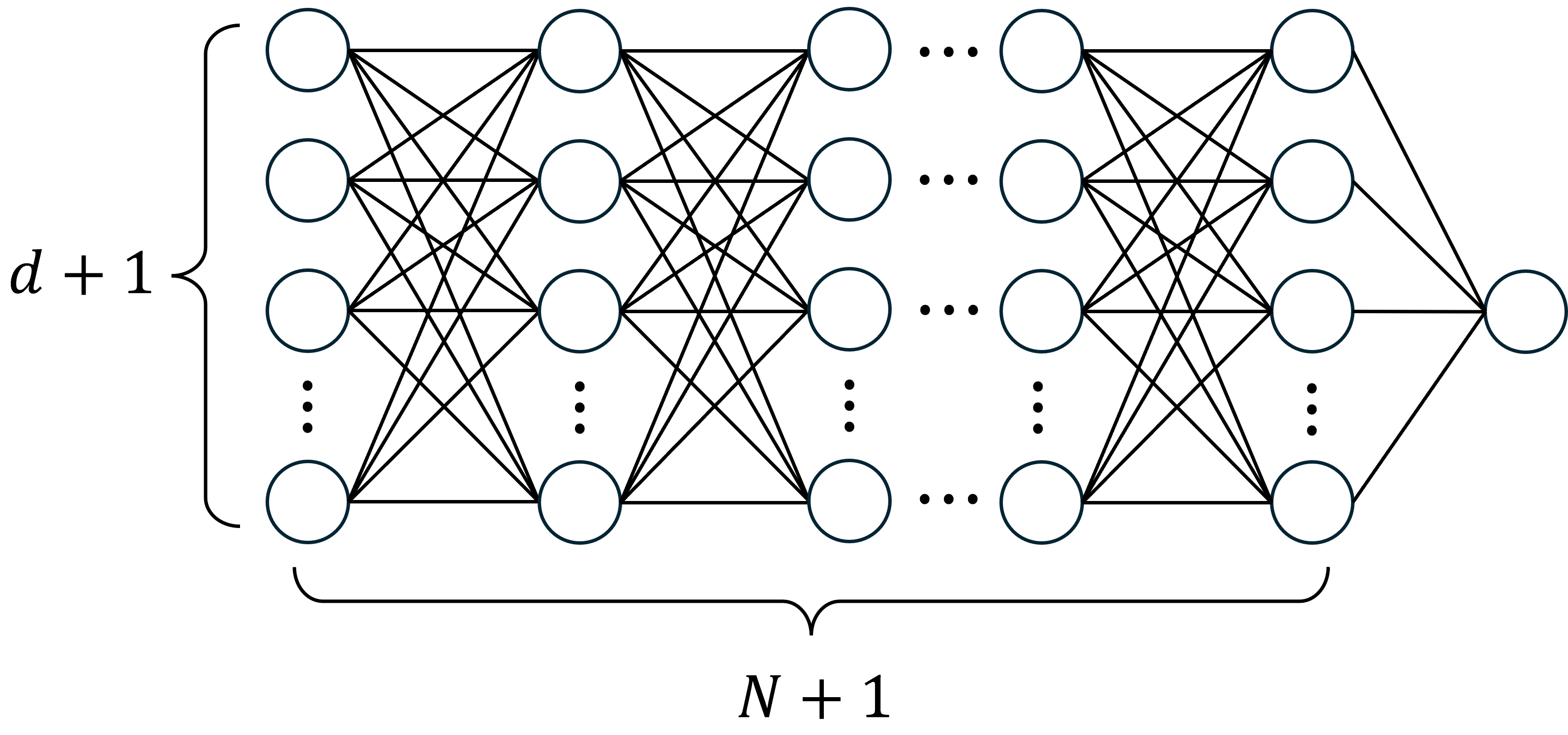
where the architecture of is defined as follows. Let be a fully-connected ReLU network of width and depth (illustrated in Figure 1), written as the composition
| (2.3) |
Here, is an affine function, and , , are functions, so-called ReLU layers, of the form
| (2.4) |
where the activation function is applied elementwise to the vector , and denotes the non-negative orthant of . Hence, the parameters of the network are the matrices , the bias vectors , and the parameters of the affine function .
Remark 2.1 (Piecewise Linear Hypersurface Approximation.).
Since the ReLU activation is a piecewise linear function it follows directly that a fully-connected ReLU network is itself a piecewise linear function, and in turn will be a piecewise linear hypersurface. However, the partition of the input domain on which the network is piecewise linear depends non-trivially on the network parameters, and the same goes for the polygonal pieces of the hypersurface.
2.1 Main Result
We here present our main approximation result and then outline the main steps taken in its proof. To express the approximation result, we first introduce the concept of a -band, which is used for describing a -dimensional neighborhood close to the exact hypersurface .
Definition 2.3 (-band).
Let where . Given a set and a non-negative constant we define the -band of over as
| (2.5) |
Remark 2.2.
If we have two continuous functions for some and the graph of restricted to a subset fulfills for some then it is clear that
| (2.6) |
Likewise, if (2.6) holds then .
Lemma 2.1 (Implicit Approximation Capacity).
Let be a scalar valued function with graph , see Defintion 2.1, and let be the -band covering , see Definition 2.3. Given a positive discretization parameter , there exists a deep fully-connected ReLU network , see Definition 2.2, of constant width and a depth of at most , such that
| (2.7) |
with a tolerance
| (2.8) |
where is a constant independent on and . The zero contour to hence satisfies
| (2.9) |
Remark 2.3 ( as the Graph of a Function).
Below, we prove a slightly stronger version of this approximation bound – Theorem 5.1. There, we by construction show that there exists a network of depth such that its zero contour coincides with the graph of a continuous piecewise linear function fulfilling the more direct error bound
| (2.10) |
which in turn implies Lemma 2.1. In practical applications, the parameters of the network are trained rather than set according to our construction, so such a corresponding to a trained network might not always exist. This, however, does not limit the applicability of the theorem since it still gives a lower bound on the approximation capacity.
2.2 Proof Outline
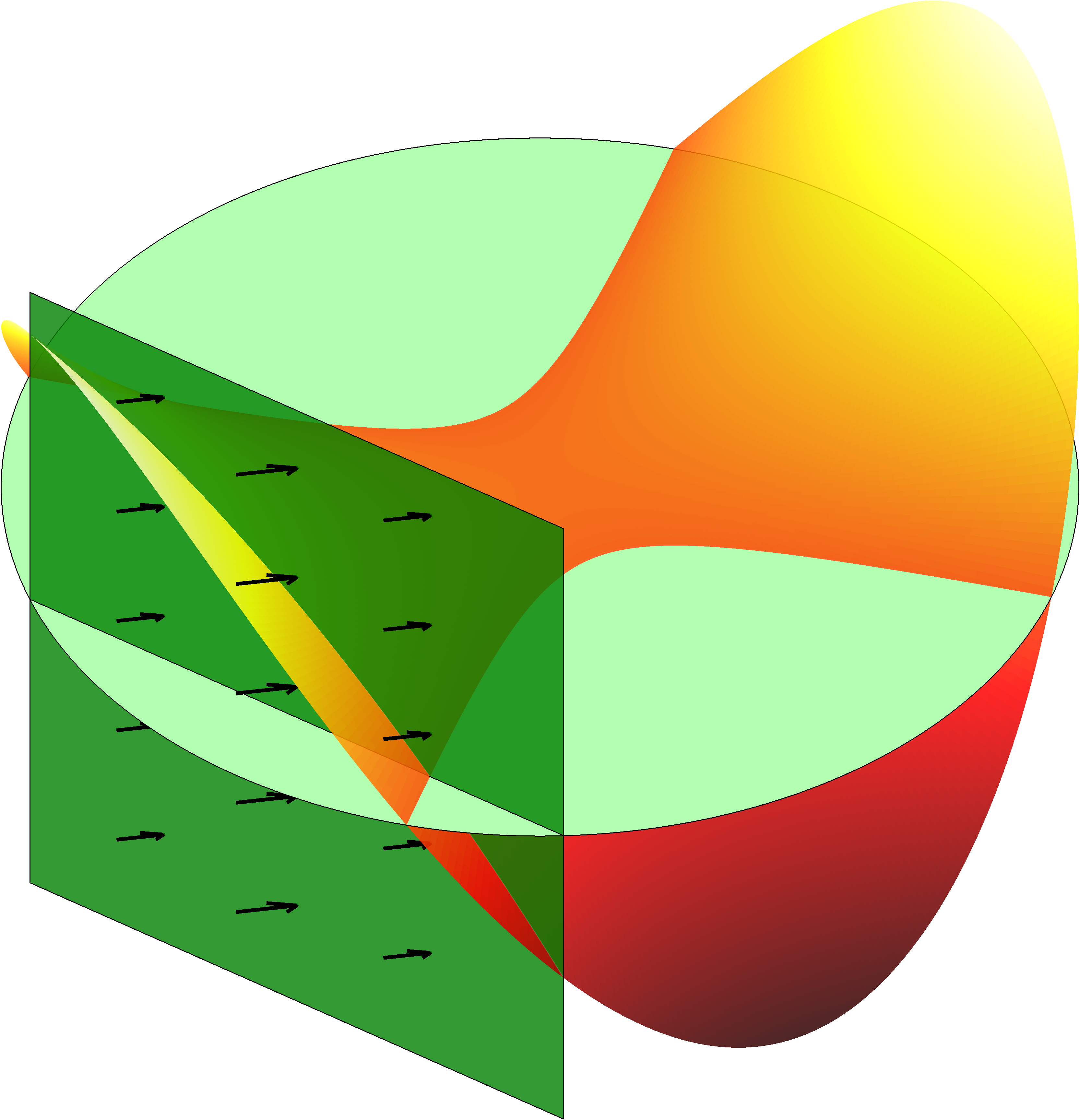
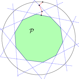
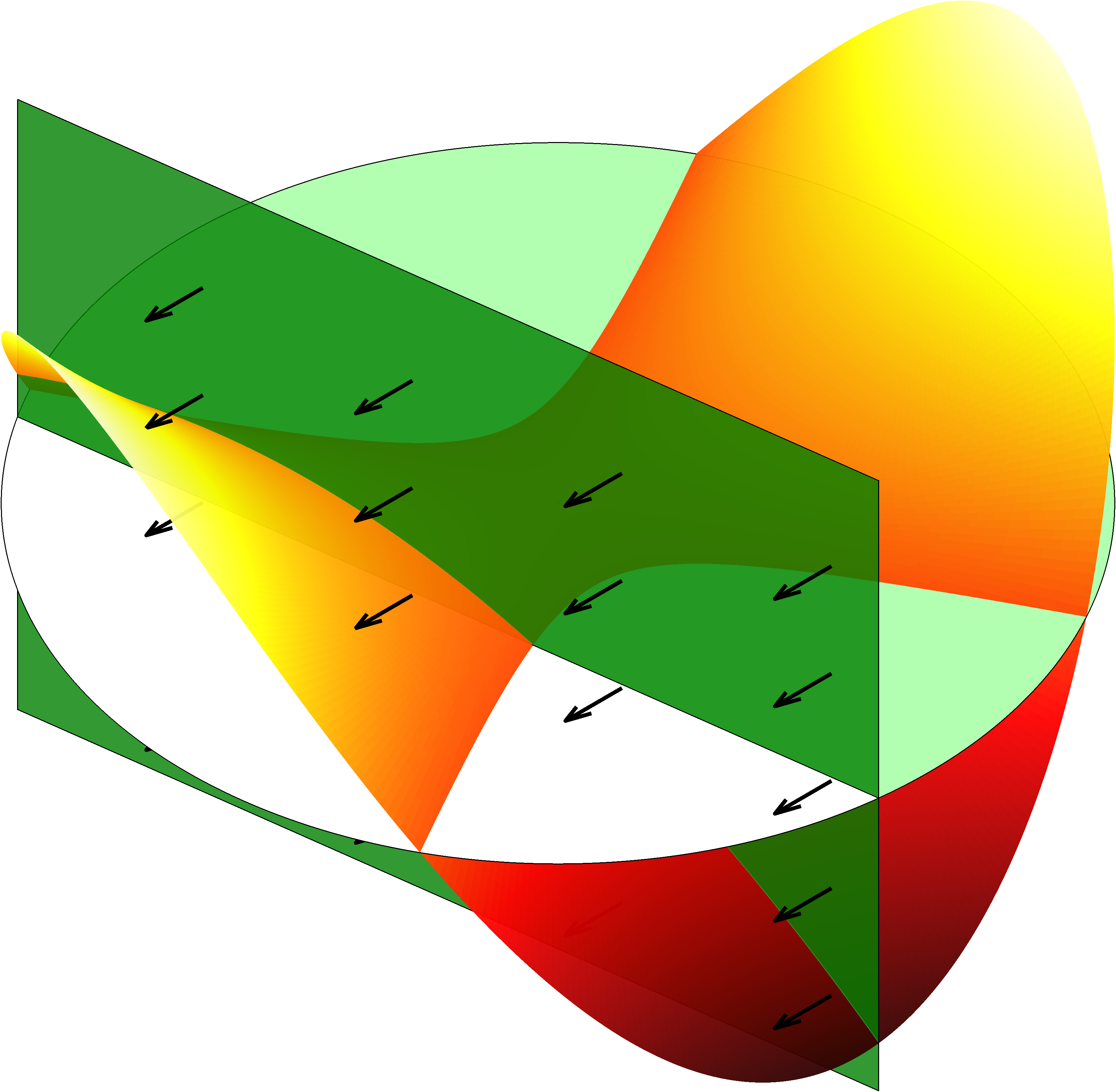
As the proof of Theorem 5.1 is rather extensive we will here give a brief description of the key steps involved and an overview of the structure of this paper. The overall idea is that the layers in the network will successively project small pieces of onto hyperplanes in a controlled way such that its image will consist of a small unaffected central piece of the original graph and a projected part contained in a small neighborhood around its boundary. We will then approximate the remaining piece by the hyperplane defined by the kernel of the last affine function in the network. As the decision boundary is the preimage of this hyperplane we will show that if the aforementioned neighborhood is small then the decision boundary will be close to .
-
•
In Section 3 we start by reexamining the geometrical structure of standard ReLU layers, detailed in [28]. Based on this geometrical description, we in Section 3.1 propose a modified network architecture, equivalent to the fully-connected ReLU networks we are interested in, with a greatly simplified action of the layers. In Section 3.2 we show that, given a half-space and a vector , such a layer can realize a map that is the identity on while is projected along onto the boundary hyperplane, see Figure 7. Hence, we can identify each layer by a half-space and a projection direction.
-
•
In Section 4 we describe how to choose each half-space and projection direction and how evolves when passing through the network. Each half-space will be chosen orthogonal to and in this setting the part of the graph projected by one layer will be contained in a neighborhood around the intersection of the graph and the corresponding hyperplane, see Figure 8.
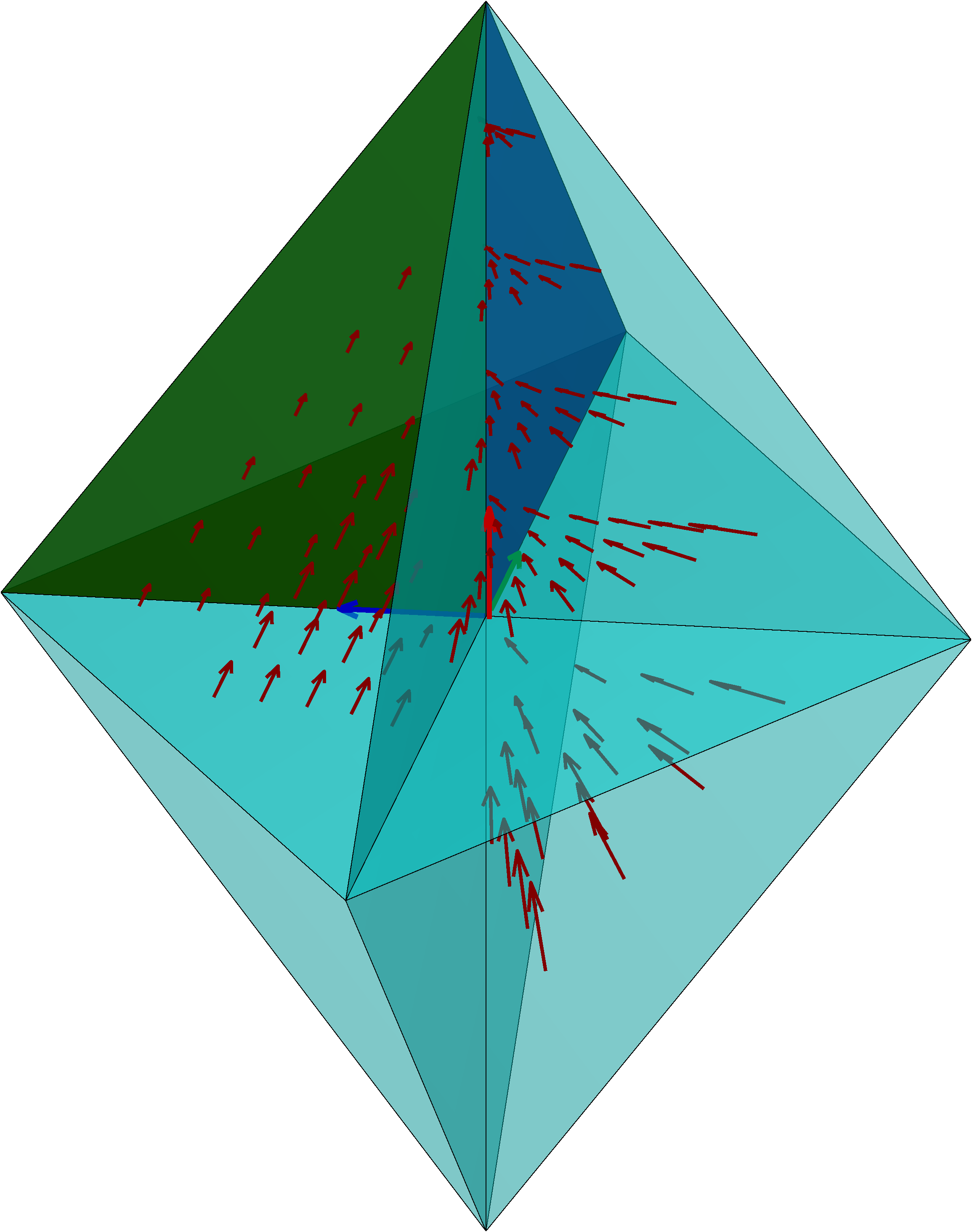
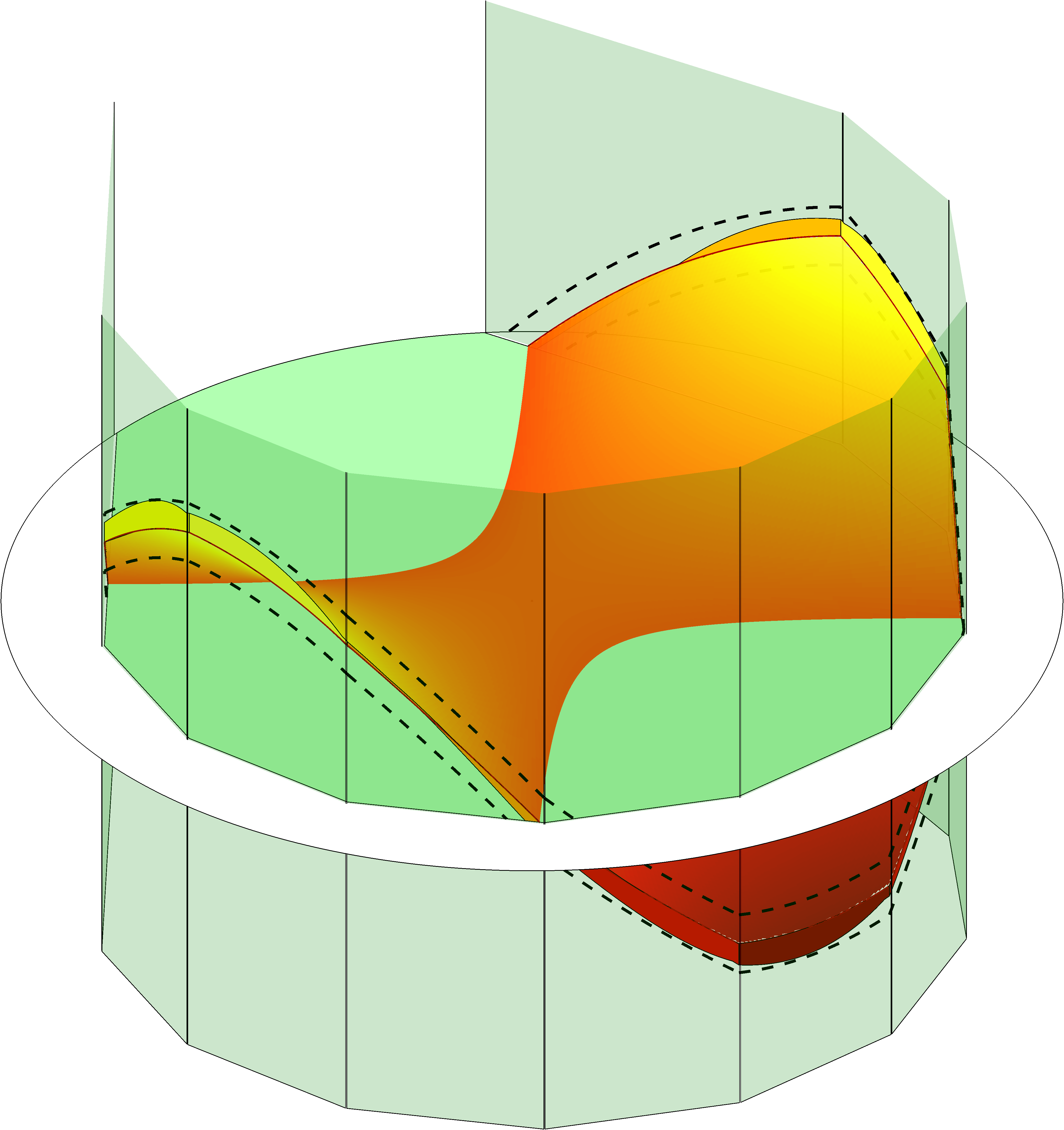
We will group the layers in the network in such a way that the half-spaces associated to each group define a convex polytope and the projected part of will be contained in a neighborhood over the boundary as depicted in Figure 15. In this way, we will get a nested sequence of polytopes and the number of them (i.e., the number of groups of layers) is chosen such that the last one is contained in the closed ball for a predefined parameter , see Figure 18. We will estimate the size of the final neighborhood we obtain.
-
•
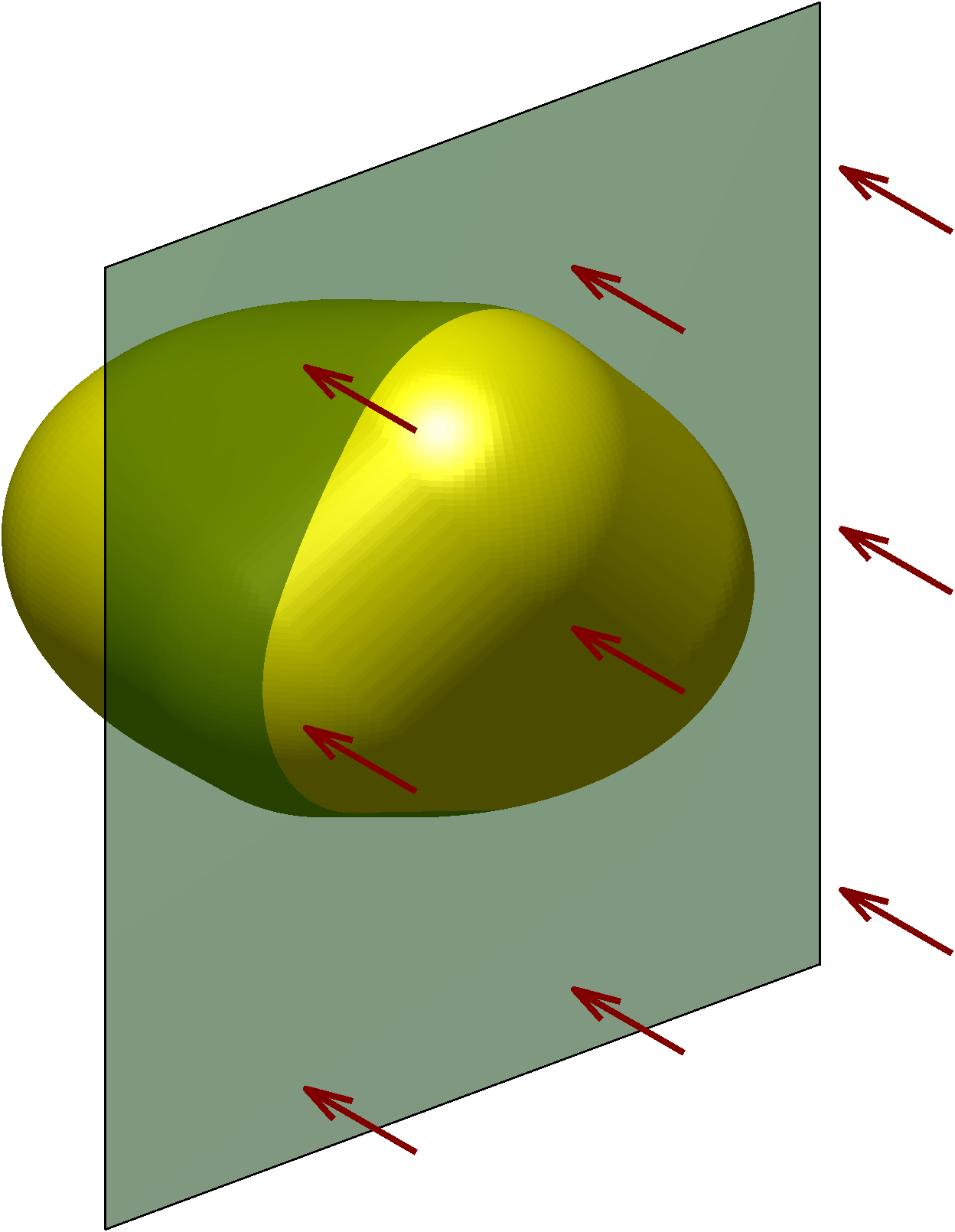
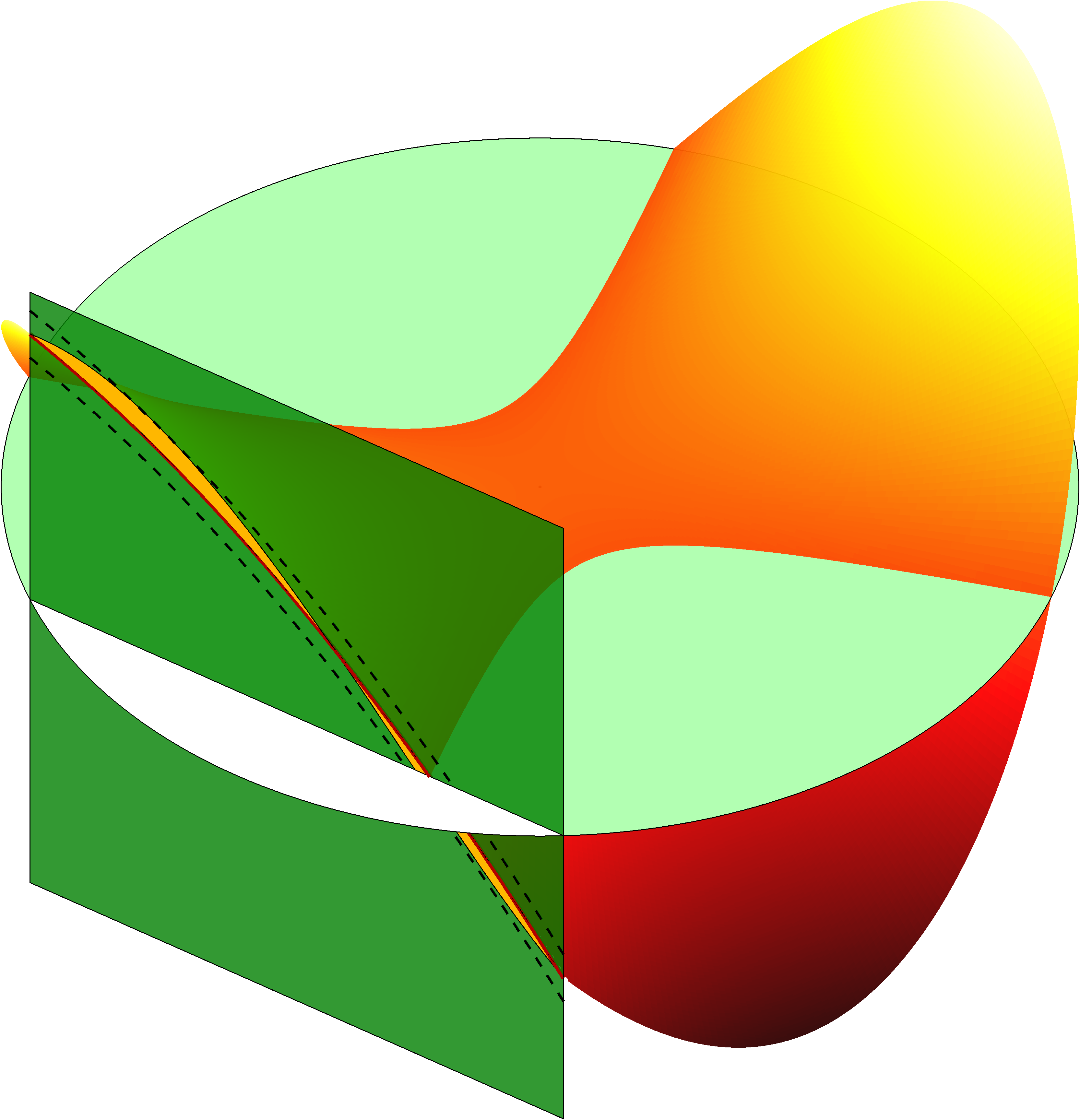
In Section 5 we start by showing how to define the last affine function in our network such that its kernel approximates over the last polytope, see Figure 19. Then, we describe the preimages of the layers in our network. We show that the resulting decision boundary will be the graph of a continuous piecewise linear function, defined on , that -approximates , see Figure 21.
2.3 Application to Binary Classification
A commonly encountered problem in machine learning is that you have a data set as a finite set of points where each point comes with a corresponding class label. When there are two possible labels we call it a binary classification problem and the task is to build a model that correctly classifies labels of unseen data. We here describe how our approximation result applies to that setting.
Binary Classification.
We assume that two bounded disjoint sets are associated with two respective classes. These two sets represent the ground truth in the sense that all possible data points from the first class are assumed to be elements in and points from the second class are always elements in . Since they are bounded, there is a point and a such that where is the -dimensional closed ball of radius centered at . Without loss of generality, we may assume that the ball is centered at the origin and simply denote it by .
If there exists a function such that
| (2.11) |
then the sign of is a classifier on and the hypersurface
| (2.12) |
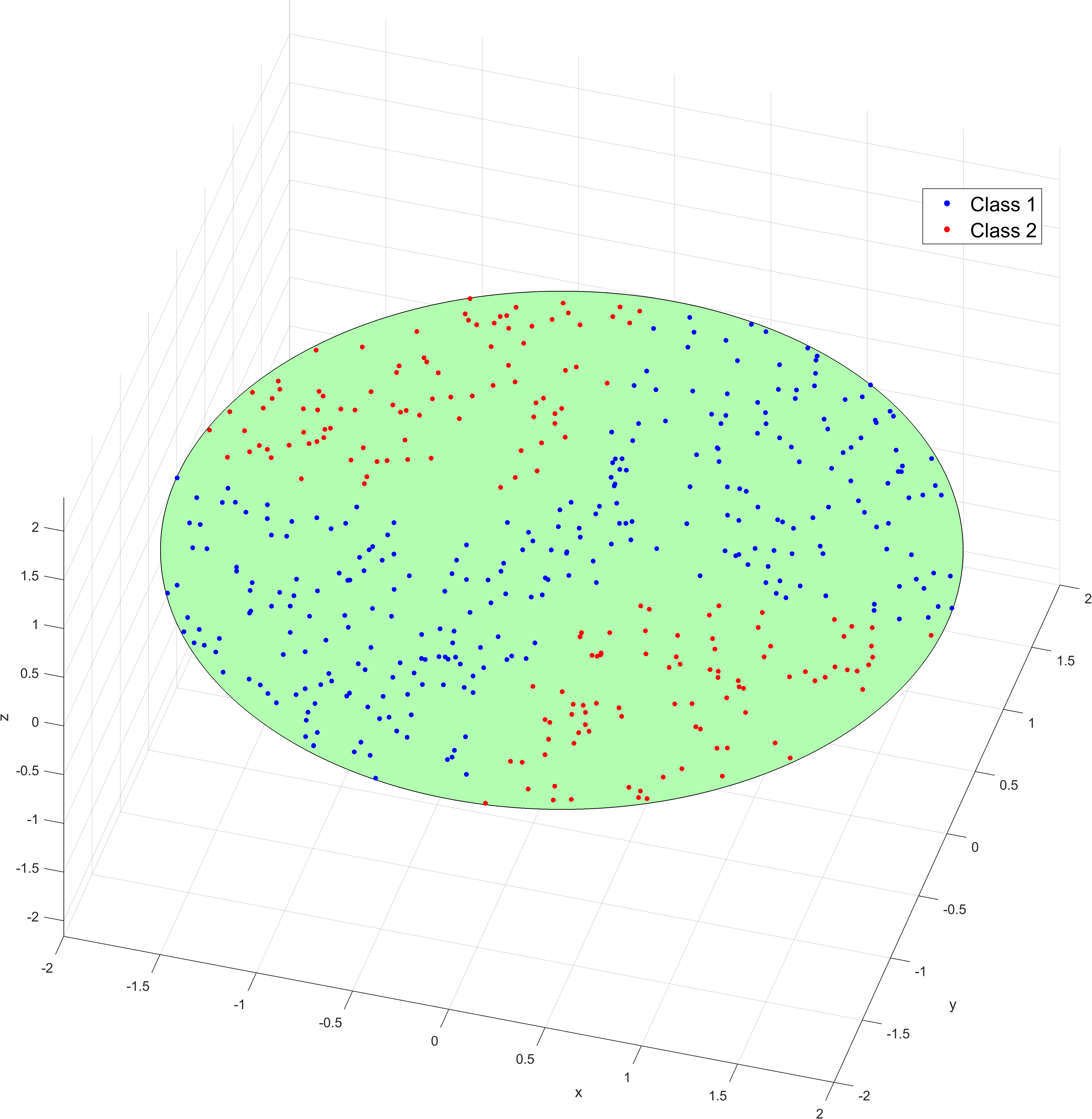
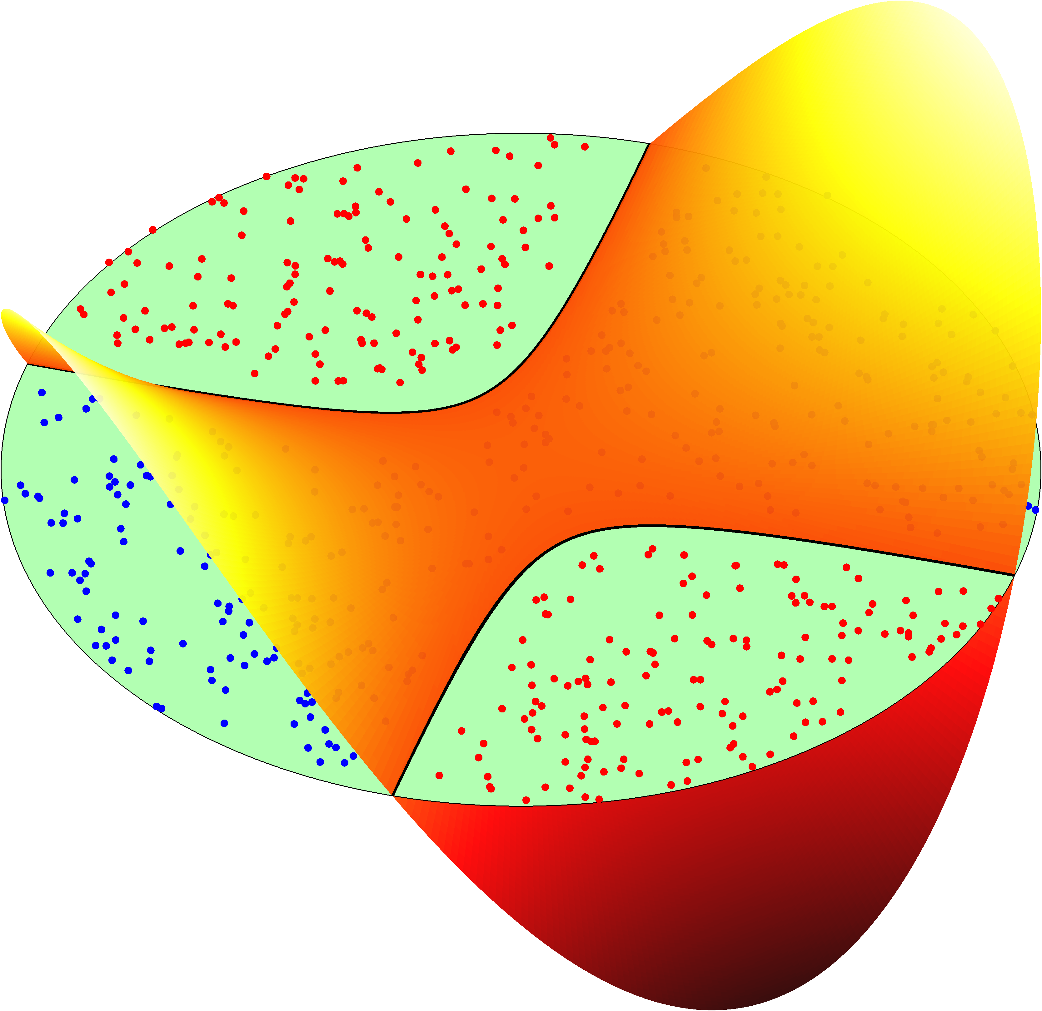
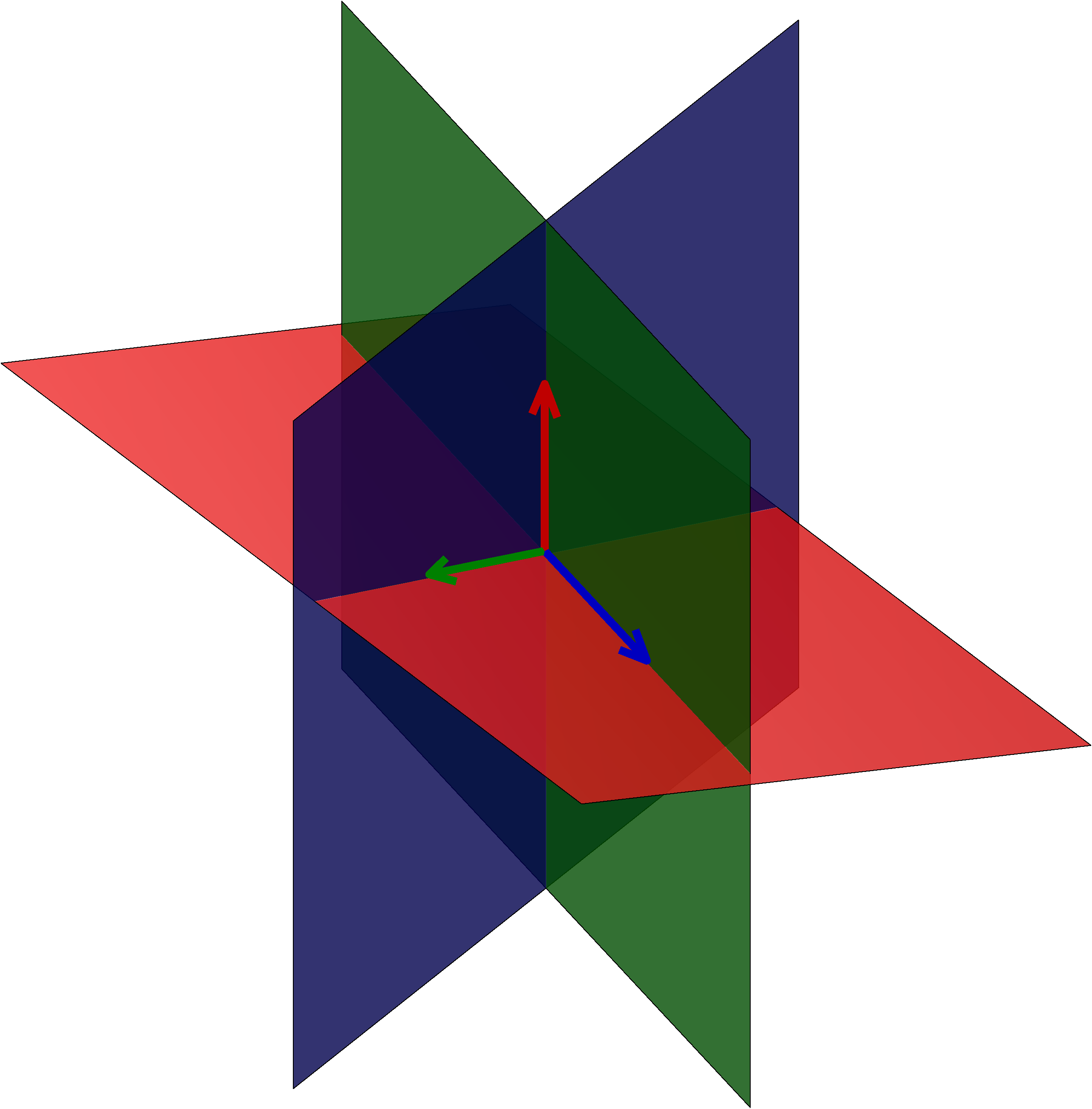
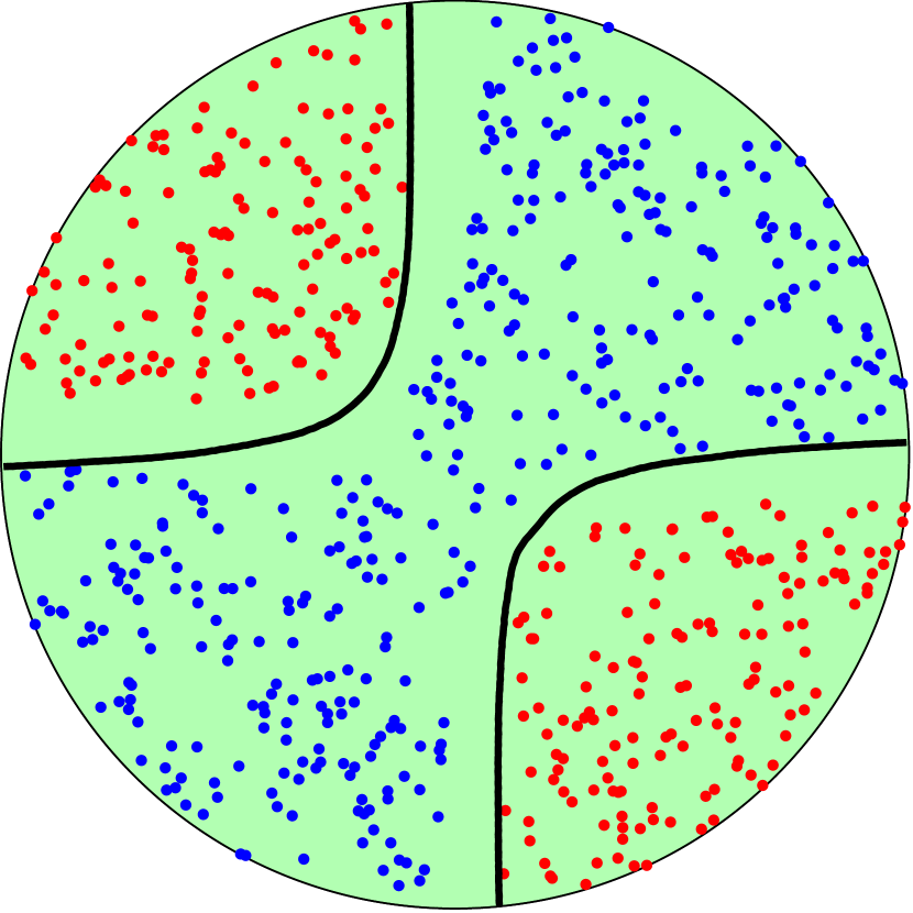
is a decision boundary separating the two datasets. Note that does not need to generate connected (or simply connected) decision regions, see the example in Figure 2. Also note that is not unique to , since, for instance, multiplied with any strictly positive function has a sign that is a classifier with the same decision boundary.
Embedment in Higher Dimension.
To each datapoint we append a , embedding the data in . This embedment in a higher dimension is required for applying our approximation result to the classification problem, and it has the well-known benefit of simplifying the topology of the decision boundary, see for instance [21, 3], where it is shown that the decision regions of networks of width less than or equal to the input dimension are always connected and unbounded (with some additional assumption on the activation functions and parameter matrices).
An alternative interpretation is that one may add a linear embedding layer in the network, mapping to , and then apply our result. This setting also occures when the data lies in a hyperplane in so that the points can be described using a -dimensional coordinate system in that plane.
The Network as a Classifier.
Given a sufficiently smooth and a tolerance , our approximation result gives the existence of a network guaranteed to correctly classify points outside an -band to . Hence, its zero contour , i.e., the network’s decision boundary, is contained within that -band.
The error bound in our approximation result directly relates to the tolerance in the additional embedding dimension, whereas a more relevant tolerance for the binary classification problem is the distance to within . For with a very small gradient over , a very small tolerance in the embedding direction is required to achieve the desired tolerance in . However, given a sufficiently regular decision boundary , there exists a corresponding smooth that is a distance function in a neighborhood to , and hence the gradient over is unit length which means that the tolerances in both the embedding dimension and in are equivalent.
Remark 2.4 (Local Accuracy).
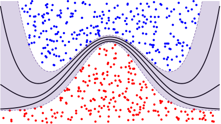
Our approximation result gives the existence of a network whose sign acts as a classifier with a tolerance everywhere throughout the domain. Most practical situations are however less strict, where the needed tolerance may vary greatly over the domain with high precision required only in a small part. This is illustrated in the example presented in Figure 4.
3 Geometrical Structure of ReLU Layers
By Definition 2.2 the network , which implicitly approximates , is constructed as a sequence of ReLU layers of the form
| (3.1) |
where and , and the entire network can be written as
| (3.2) |
for some , where is an affine function. In our earlier contribution [28], we showed that maps on the form (3.1) can be described geometrically as a projection onto a -dimensional polyhedral cone followed by an affine transformation mapping the cone onto the non-negative orthant . We will now give a brief summary of the description we provided there.
Dual Vectors.
For now, we drop the indices on the ReLU layer in (3.1) and just consider one single map . We define the index set and we will assume that the matrix has full rank. Let be the :th row vector in and the :th component of . Now we can define a set of dual vectors by the equation
| (3.3) |
It follows that these dual vectors span since has full rank by assumption. Further, we also know that there is a point which is the unique solution to the linear system of equations
| (3.4) |
Partition.
To understand the map geometrically we introduce a partition of using the dual vectors. Given two disjoint index subsets we define the set
| (3.5) |
Every point in belongs to precisely one set for a suitable pair . Thus, the family of sets of the form in (3.5) constitutes a partition of . Note that the closure of the special set defines a -dimensional polyhedral cone with apex at . We will denote this cone simply by
| (3.6) |
Projection on Cones.
We showed in [28] that this polyhedral cone plays a central role in understanding the action of the map geometrically. More precisely, we can decompose the map as
| (3.7) |
where
-
•
is a surjective map projecting onto the cone ,
-
•
is a bijective affine transformation given by mapping to .
We call this decomposition of its conical decomposition. Thus, apart from a translation, the nonlinearity of is fully captured by the projection which is piecewise defined on the sets in the following way. For a point with expansion
| (3.8) |
for some positive scalars , the projection is defined as
| (3.9) |
and by the equations (3.3)-(3.4) we get
| (3.10) |
where is the :th Euclidean basis vector. Thus, projects onto the set which is a -dimensional face of the polyhedral cone and the projection is parallel to the subspace spanned by . Hence, all points outside the cone will be projected onto some part of its boundary, and points in the cone will be left unaffected by . Thus, reduces to an affine map on . This gives a complete geometrical description of the action of the ReLU layer . A polyhedral cone and the corresponding projection is depicted in Figure 5.
Geometrical Interpretation.
The equations (3.3) and (3.6) give algebraic definitions of the dual vectors and the cone respectively. To see how these objects can be interpreted geometrically we can define the open half-spaces
| (3.11) |
with the corresponding hyperplanes
| (3.12) |
as boundaries. Note that the row vector is a normal to . We can now express the cone as the intersection of these half-spaces
| (3.13) |
Thus, each hyperplane is tangent to one facet of the polyhedral cone. Moreover, if we define the lines
| (3.14) |
it follows that the dual vector is parallel to the line and scaled such that , see Figure 6. Thus, the directions of the projection on each set is determined by the different lines of intersections (the 1-dimensional faces of ) in the hyperplane arrangement.
3.1 A Modified Network Architecture
With the conical decomposition (3.7) in mind we will now introduce a modified network architecture where we retain the projection but disregard the affine transformation in each ReLU layer. Thus, we consider networks of the form
| (3.15) |
where for are projections and is an affine function.
Here, each is a polyhedral cone
| (3.16) |
defined by an apex and a set of linearly independent dual vectors for . Recall that the definition of such a projection is given by equation (3.9) and it is piecewise defined on the corresponding partition (3.5) generated by the dual vectors in each layer. Since we have disregarded the affine maps in this network, each layer is completely determined by and .
Remark 3.1.
By construction, it is clear that scaling the dual vectors by a positive constant or permuting them does not change the cone. Hence, there are many different affine maps generating the same polyhedral cone.
We introduce this network architecture since it will simplify the proof of the approximation result later. In fact, for every network of the form in (3.15) there is a fully-connected ReLU network (of the form defined in (3.2)) computing the same function.
Lemma 3.1 (Equivalence of Architectures).
Given a network as in (3.15), then there is a fully-connected ReLU network with the same number of layers such that
| (3.17) |
-
Proof.To see this, suppose is a network of the form in (3.15). We want to find a fully-connected ReLU network of the form (3.2) such that for all . We start by letting denote the polyhedral cone corresponding to layer in (3.15). For each let be one of the possible affine maps generating . Each such affine map is invertible since the vectors generating the cone are linearly independent (the cone is non-degenerate). Then, as inverses and compositions of affine maps are themselves affine maps we can define the fully-connected ReLU layer as
(3.18) with (the identity map). Similar to the conical decomposition described in Section 3 we can decompose as
(3.19) We can interpret this decomposition as follows:
-
First, maps back onto the previous cone, namely .
-
Then, projects onto the cone associated to the affine map .
-
At last, maps onto .
By construction, we then get that the composition of all ReLU layers reduces to
(3.20) Hence, if let we can conclude that for all . ∎
-
Thus, if we can show that a network of the modified architecture can approximate by its decision boundary then the same result holds for a fully-connected ReLU network as well.
3.2 Restrictions to Bounded Sets
We will now show how the modified layers can be reduced to projections on hyperplanes when restricted to bounded sets. First, consider a projection and the set for some . This set is an element in the partition of defined by (3.5). It is the set satisfying for and . Thus, the action of on this set is precisely
| (3.21) |
as projects every point in along onto the facet of the cone and this facet is also contained in the hyperplane defined in (3.12). Recall that the projection direction is parallel to the line given by the intersection of the set of the remaining hyperplanes when is removed.
Lemma 3.2 (Projections on Hyperplanes).
Let be a bounded set. Given a closed half-space with the hyperplane as its boundary and a vector not parallel to , we can construct a projection defined as in (3.9) such that projects on along while acting as the identity on .
The proof of Lemma 3.2 can be found in Appendix A.1. Figure 7(a) illustrates such a hyperplane projection and the idea is that we can always orient and shape the cone such that the two maps coincide on a bounded set, as in Figure 7(b).
As is bounded for any positive real number we can construct layers such that their actions, restricted to this set, can be described by a projection direction and a halfspace in accordance with Lemma 3.2. Hence, we will assume is large enough such that all sets we will be considering is contained in .
4 Projecting the Graph
4.1 A Single Projection
The procedure will be to repeatedly project parts of by cutting off small pieces of the domain by the half-spaces associated to the layers. We will always choose these half-spaces orthogonal to . Such an half-space in can be decomposed as where is a half-space in . Similarly, the boundary hyperplane of can then be written as where is the boundary hyperplane of . We will continue to use bold symbols to denote the associated half-space/hyperplane in while the same symbols without the bold typesetting will refer to the corresponding half-space/hyperplane in .
We will now consider the image of by a single projection . In this setting, will be projected while will be left unchanged when applying . After the projection, the set will lie in a neighborhood in around the intersection as depicted in Figure 8. These neighborhoods are formally described using the -band , see Definition 2.3, which pads over a set with all points within a tolerance in the -direction. Figure 9 illustrates the resulting -band in the projection-plane after the mapping depicted in Figure 8.
With this notation, we will have
| (4.1) | ||||
for some . As we will repeatedly cut off the domain by half-spaces the image of after several projections will consist of one unaffected part as the graph of the restriction of to some subset and a projected part contained in an -band of over . The set is the set in contained in every half-space associated to the projections. Figure 10 shows an example of the image of under a composition of a number of projections.
To suppress the notation, given a set we let denote the part of the graph of defined by
| (4.2) |
Consider the graph for some . We would like to estimate the size of the resulting -band after one projection of . Therefore, we will now take a closer look at how a point on is mapped for a special choice of projection direction .
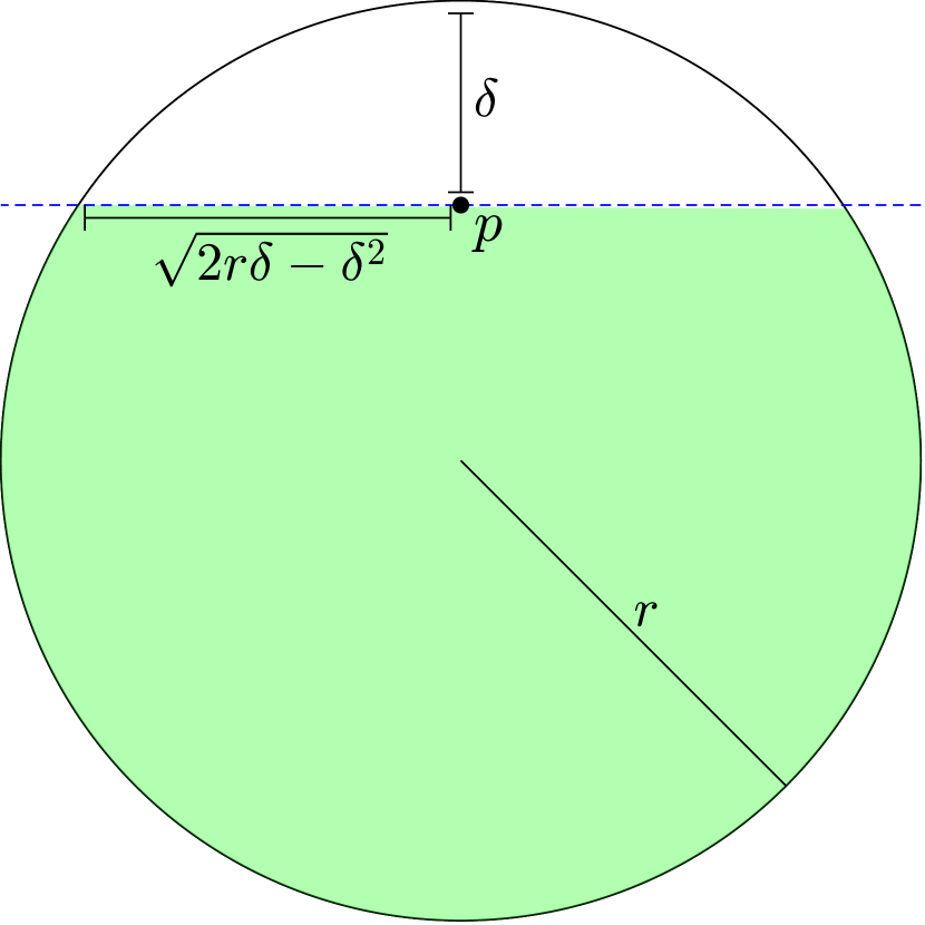
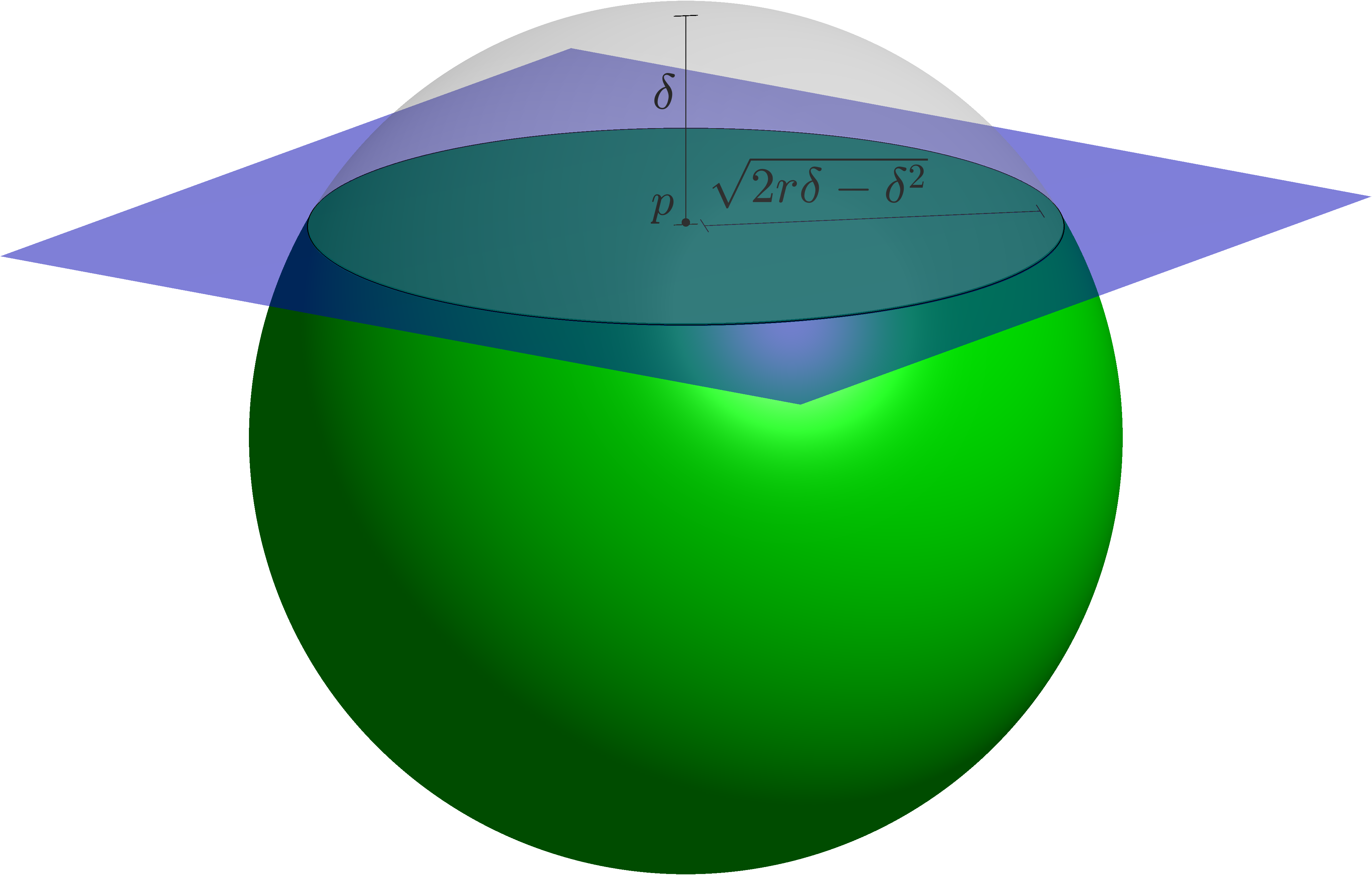
Mapping a Point.
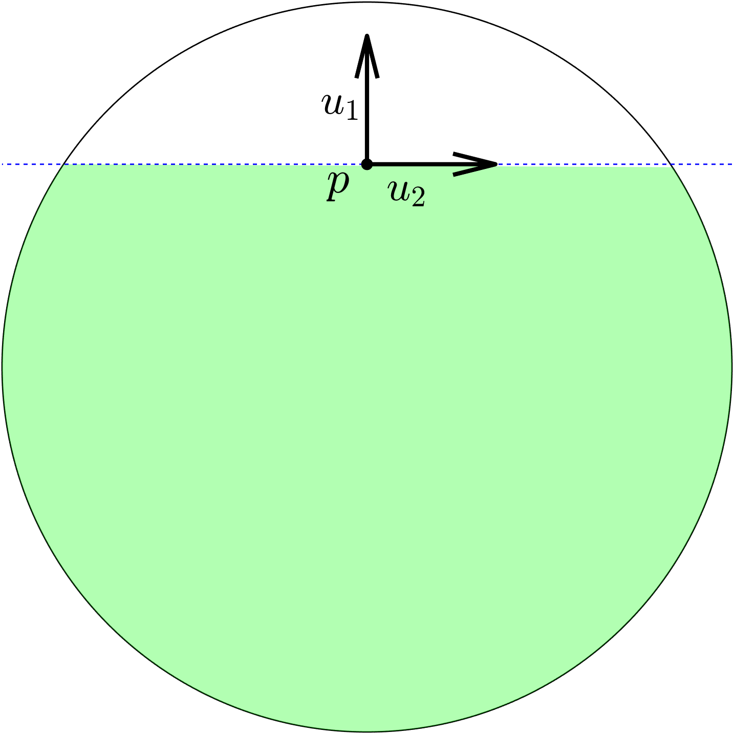
Let be the half-space and boundary hyperplane associated to a layer respectively and let be the inward pointing unit normal to . Assume that is tangent to the ball of radius , for some , concentric with . Then, is a spherical cap of height and the base is a dimensional ball of radius with a center point denoted by . The geometrical situations for and are depicted in Figure 11.
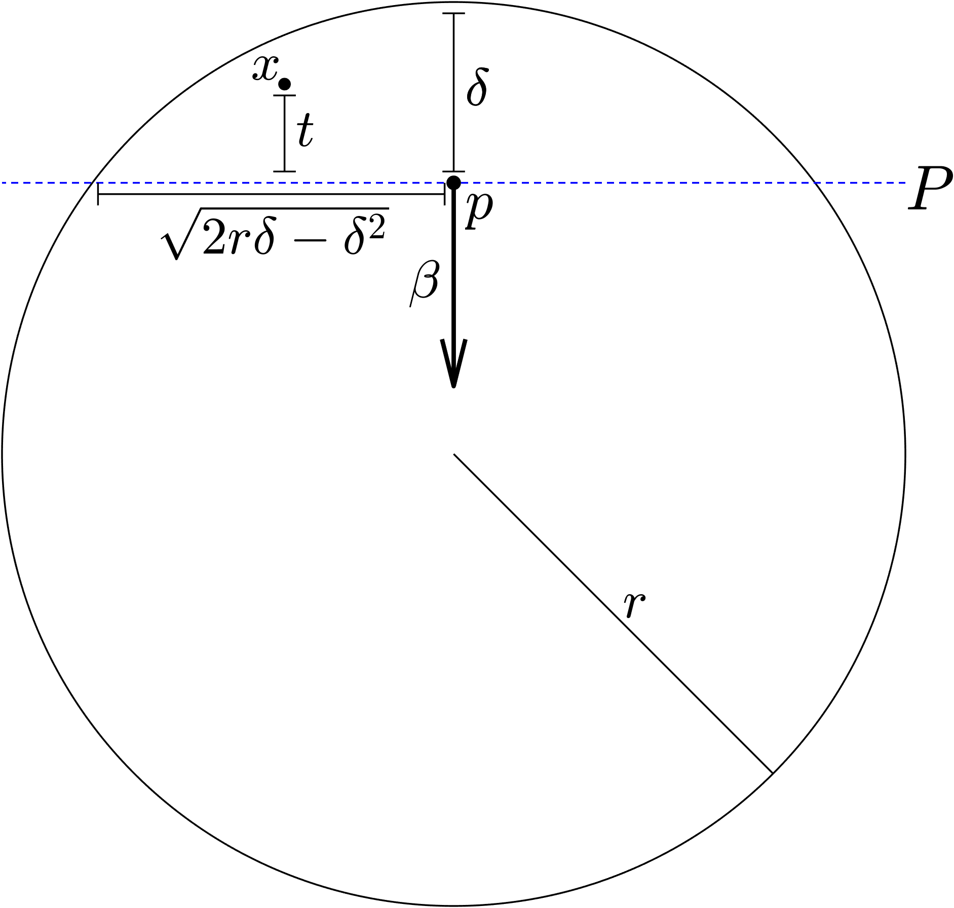
Now, assume and let . Then, the point will be projected on by along a direction . Suppose now that we choose the projection direction as
| (4.3) |
where is the directional derivative of at the center point with respect to the unit normal . Then, if is the distance between and we can express the action of on this point as
| (4.4) |
Since is the height of the spherical cap, we know that . Figure 12 shows the geometrical setup in the 2-dimensional plane spanned by and the vector pointing to .
In particular, the point will mapped according to
| (4.5) |
The Size of the -band.
Note that the first coordinates of the image in (4.5) is and the value of at this point is precisely . Therefore we introduce the quantity
| (4.6) |
measuring the offset between the projection of and the corresponding point on the graph . Note that depends on . If we would set
| (4.7) |
then as is an upper bound on the offset between the graph over and the projected points. Therefore, we will now continue by estimating the quantity in (4.6). We have the following proposition.
Proposition 4.1.
Suppose and . If , then
| (4.8) |
where is a constant independent of , and .
The proof of Proposition 4.1 can be found in Appendix A.2. The idea is to use Taylor’s theorem and the fact that the second order derivatives of are bounded by assumption. The following corollary follows directly from Proposition 4.1.
Corollary 4.1.
Let be the height of the spherical cap whose base has center and let be the inward pointing unit normal to . If and we choose the projection direction then
| (4.9) |
where for a constant .
-
Proof.From Proposition 4.1 we know that the offset between the projection of a point where and the corresponding point in the intersection satisfies the inequality
(4.10) where is the distance between and . Taking the supremum on both sides of the inequality over all in we get an upper bound on the maximal offset of the projected points and the graph in the hyperplane. By noting that is the only factor dependent on on the right hand side of the inequality and for all we get
(4.11) and the corollary follows. ∎
Both Proposition 4.1 and Corollary 4.1 hold as long as . If we get a more favorable scaling of , see Remark A.2 in Appendix A.2. We will assume that henceforth.
4.2 Projection on a Polytope
In the previous section we saw the effect on after a single projection. Now, we will turn to the more general case when we apply a group of layers. To that end, let be defined by the composition
| (4.12) |
for some . As before, we denote by , the associated half-space and hyperplane to layer respectively and we let be the inward pointing unit normal to .
Construction.
We will define the layers such that all the corresponding hyperplanes are tangents to for some and each half-space contains the origin. Thus, we can express them explicitly as
| (4.13) | ||||
Further, let be the center point of the base of the spherical cap so that the projection direction of layer is given by . Note that is precisely the point where touches . The intersection of these half-spaces will be a convex polytope and we will assume it satisfies
| (4.14) |
The first inclusion always holds as each half-space contains by construction, but for the second inclusion to hold we assume we have enough half-spaces and that they are distributed properly. Later, we will give a more detailed construction assuring the validity of the second inclusion as well, see Figure 13.
Mapping a Point.
In this setting a point , with , may be projected several times. Therefore, we introduce the notation
| (4.15) | ||||
so that . Then, the sequence describes the trajectory of the point in obtained by applying the layers in successively. Note that this trajectory is in general dependent on the order of the layers in (4.12). If we now let
| (4.16) |
then by (4.4) we have
| (4.17) |
Thus, if then so . Otherwise, and then . The sequence defines a piecewise linear path in and its total length is given by
| (4.18) |
An example of such a path is illustrated in Figure 14.
By (4.14) we can write and as is the identity on , by the definition of , we have . Now, we would like to show that the projected part of the graph lies within an -band of over (recall Definition 2.3), i.e.,
| (4.19) |
and also estimate the size of . We do this in two steps.
-
1.
We derive a condition on guaranteeing that . This will assure that a point with is mapped to a point in the set for some .
-
2.
We continue by deriving a uniform bound on , independent of the starting point , such that the inclusion in (4.19) holds. We will do this by estimating as this quantity measures the offset between the graph over and the image of the point under .
We will start by deriving a constraint on in terms of guaranteeing that . In doing so, we will need the following lemma.
Lemma 4.1.
If two hyperplanes and in (4.13) intersect in then
| (4.20) |
The proof can be found in Appendix A.2. We are now ready to prove the following lemma giving a constraint on .
Lemma 4.2 (-Condition).
If satisfies the inequality
| (4.21) |
then .
-
Proof.Consider the sequence defined by (4.17) where . Since it is clear that cannot be contained in the interior for any because every time some point in the sequence is projected, it will be projected onto a supporting hyperplane to . If we can show that
(4.22) for all , then in particular and hence .
We will now show, by induction on , that if fulfills (4.21) then (4.22) holds. Clearly, by (4.17). Suppose now that . Again, by (4.17) we have that , but we also need for every .
-
If then , and in this case we can directly conclude that (4.22) holds by the hypothesis.
-
If instead , then . Now, let and consider the case when . Then, we can directly conclude that . However, we will have to investigate the case when .
This situation arises when the two hyperplanes and intersect inside . Thus, we need to show that , i.e., whenever and intersect inside . Using (4.17) we can rewrite this condition as
(4.23) but since by assumption we have that . As in the case we are considering, a sufficient condition is to ensure that
(4.24) By Lemma 4.1, we know that . Now, if satisfies (4.21) then it follows that . Hence, this condition on guarantees the validity of (4.24) which in turn assures the relation in (4.22).
Then it follows by induction that as desired. ∎
-
Under the restriction provided in Lemma 4.2 all points will be mapped to as long as is sufficiently large.
The Size of the -band.
We proceed by deriving a bound on the quantity describing how much the last value deviates from the function value at the endpoint . This will help us estimate the size of the resulting -band. Even though we cannot directly apply Proposition 4.1, as it is only valid for a single projection, it will be useful in proving the following lemma.
Lemma 4.3.
The following inequality holds
| (4.25) |
where is the length of the path defined by the sequence .
Lemma 4.3 shows that the deviation between the graph and the image of a point under the projections depends on the total path length. In the proof, found in Appendix A.2, Proposition 4.1 is repeatedly applied. We will now continue by estimating the path length. First, we have the following result.
Lemma 4.4.
Let be defined as in (4.16), then
| (4.26) |
The proof is based on a geometrical argument and can be found in Appendix A.2. Using Lemma 4.4, we can easily bound the sum in (4.18) and thus give an upper bound on .
Lemma 4.5.
If then
| (4.27) |
for a constant independent of , and .
-
Proof.From Lemma 4.4 we get
(4.28) but we know that so . Moreover, and since , we have that . Hence, we arrive at
(4.29) For values of close to the right hand side of the inequality above gets very large. On the other hand, we know that must be chosen such that it satisfies the constraint in (4.21) to ensure . It is easily seen that for values of in this range, we have
(4.30) Together with (4.29) we get bound
(4.31) where . Then, by Lemma 4.3 we arrive at
(4.32) with . ∎
We summarize the findings of this section in the following proposition characterizing the image of under the map , also illustrated in Figure 15.
Proposition 4.2 (Image of the Graph).
Let be defined by where the corresponding hyperplanes to the layers are all tangent to for some satisfying . Suppose the convex polytope , obtained as the intersection of the half-spaces associated to the layers, satisfies . Then, our choice of the projection directions for each layer in yields
| (4.33) | ||||
where for a constant independent of , and .
4.3 Projections on a Sequence of Polytopes
In the preceding section we considered the case when the graph of restricted to the ball of a general radius is projected by a chain of layers where the corresponding half-spaces defined a polytope tangent to the concentric ball . We showed that the projected part will be contained in the -band of over the boundary of the polytope if as long as . We will now continue by describing a procedure to project the graph repeatedly in a similar way.
Sequence of Polytopes.
Note that we can express a network of the form in (3.15) as
| (4.36) |
where each is a composition of layers
| (4.37) |
The total number of layers in the network is then
| (4.38) |
We denote the -dimensional half-space and hyperplane associated to layer by and respectively, where and . For every , we can now define the convex polytope
| (4.39) |
assumed to be bounded and to each such polytope we let
| (4.40) |
Thus, is the radius of the smallest closed ball containing . To simplify the notation we will let (recall that is the domain of ) and . The goal is to construct each such that its image under the composition of all maps satisfies
| (4.41) |
for some we want to estimate. Moreover, we would like
| (4.42) |
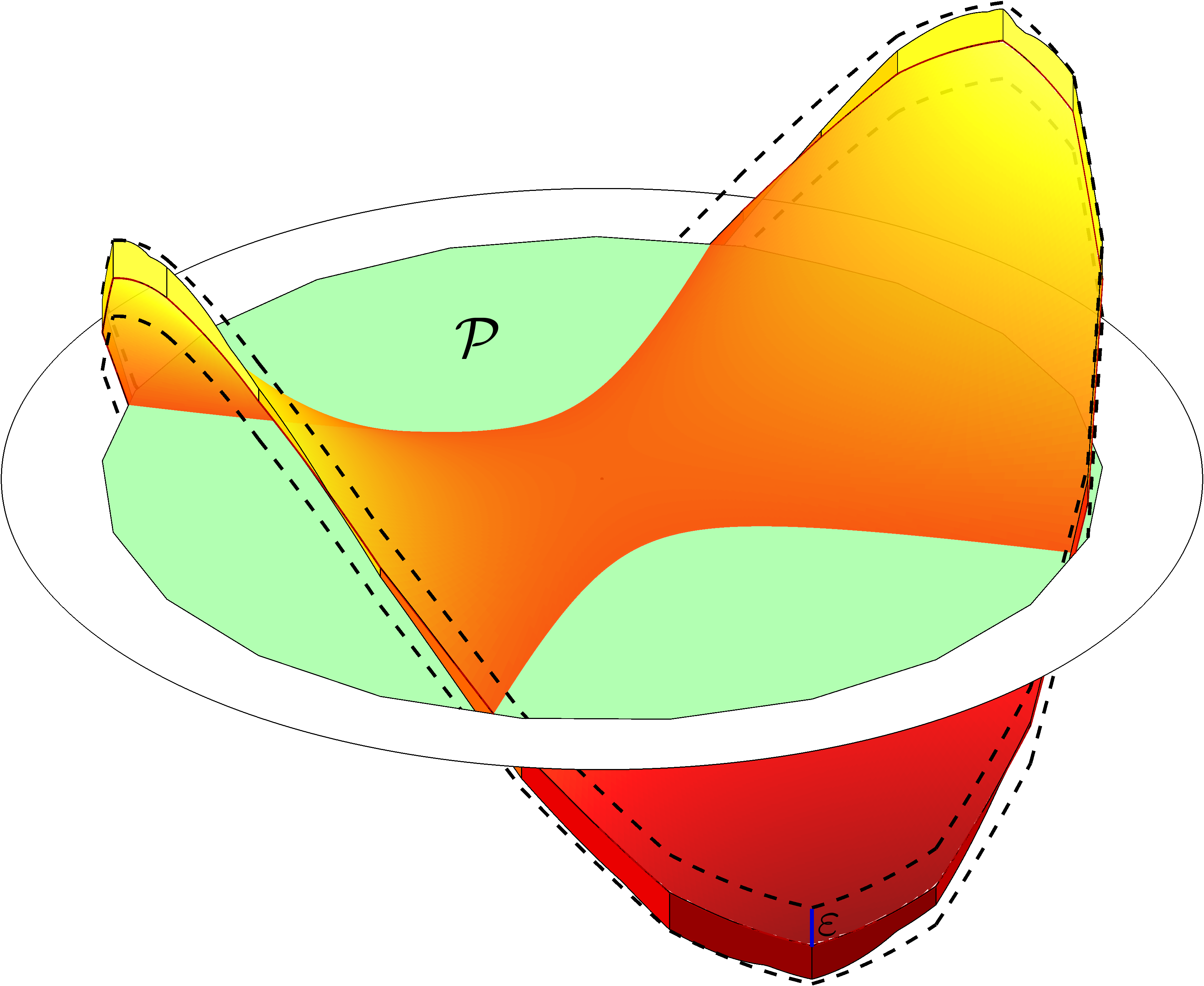
so that can be made arbitrarily small by choosing , and thus the number of layers , large enough. If is sufficiently small, we can approximate the remaining part of the graph, namely , by the hyperplane where is the last affine map in (4.36). Then, as the decision boundary is the preimage of we will see that it will approximate on to an accuracy related to the value of in (4.41).
Construction.
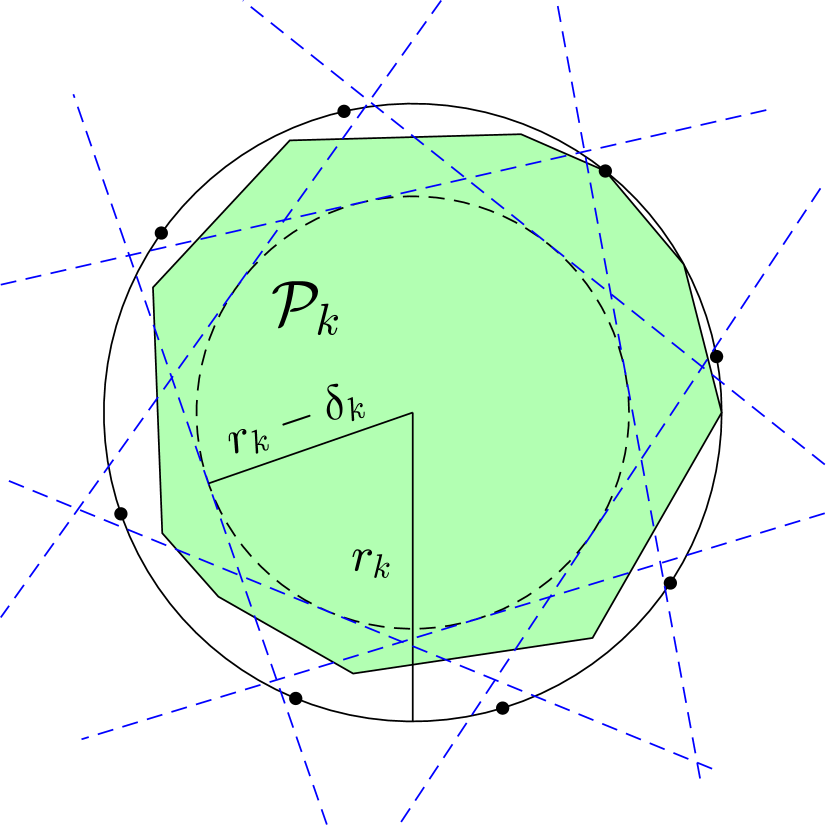
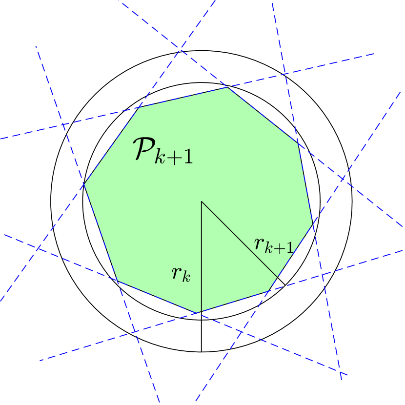
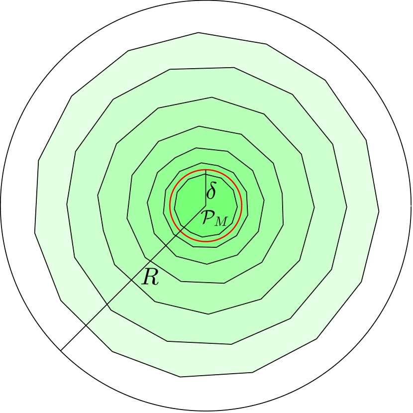
We will now describe how we construct each polytope by specifying each half-space in their definition (4.39). The main idea is similar to the construction of the polytope in Section 4.2. We will define them recursively. Given we construct by letting the half-spaces associated to the layers in be tangent to a smaller ball of radius for some . We will use the notion of an -net.
Definition 4.1 (-net).
Given a bounded set we say that a finite subset is an -net of if for all points there is a point such that .
Remark 4.2.
Given and , let be an -net of the sphere enclosing . Define (we will give an upper bound on this quantity later) and label the points as . To each point we define the half-space in the following way. Let be the point on the sphere intersecting the ray from the origin passing through . Define such that it is tangent to precisely at and oriented such that it contains the origin.
Thus, is a spherical cap of height where is the center of its base. Figure 16 illustrates how the half-spaces are defined given the -net.
In this way, is constructed by taking the intersection of tangential half-spaces to and
| (4.43) |
The reason we introduce an index on the parameter is that we have to guarantee that the condition (4.21) holds for all to get well-behaved projections. Given a predefined discretization parameter we then define according to
| (4.44) |
Thus, when the radius is sufficiently small we will need to reduce .
Properties of the Construction.
Now, in order to prove (4.41) and (4.42), we will start by proving that and give a lower bound on , i.e., how much the radii decrease at each step. Then we will proceed by proving the inclusion by utilizing Proposition 4.2 repeatedly.
To guarantee that we get a nested sequence of polytopes we will need to choose small enough. For our purpose, choosing
| (4.45) |
will be sufficient. First, we have the following lemma.
Lemma 4.6.
The construction of the polytopes guarantees that the inclusions
| (4.46) |
hold for all .
Thus, each polytope lies inside the ball enclosing the previous polytope. The proof is presented in Appendix A.2. We can now prove the following lemma giving a lower bound on the reduction of the radii and guaranteeing that the polytopes are nested.
Lemma 4.7.
The polytopes and the radii satisfy
| (4.47) | ||||
for all .
-
Proof.We first show . Recall the definition of in (4.40). From Lemma 4.6 we have . Let be a point fulfilling . Clearly, will be a vertex on the convex polytope and will thus be contained in the intersection of a subset of the boundary hyperplanes associated to .
If is the closest point on the sphere to the point , then . Next, let be the closest point to , then it follows that . Define , then since is an -net of and let be the orthogonal projection of onto . Figure 17 shows the geometrical setup.

(a) 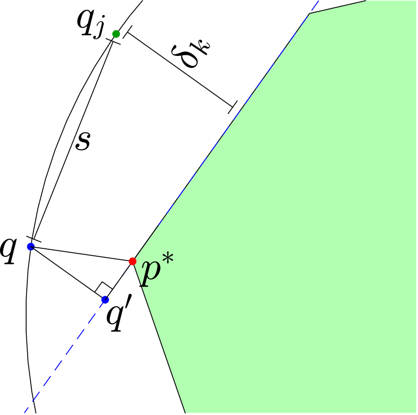
(b) Figure 17: Estimating the Radius. (a) The point is a vertex in satisfying . If we let be the closest point to on , then the closest point in the -net will be within a distance from . (b) We can give a lower bound on by computing the length where is the orthogonal projection of onto the hyperplane .
Consider the right triangle with vertices at , and . As the line between and is the hypotenuse in this triangle we have that . Moreover, since we have that . This gives us the bound . By inserting we obtain
| (4.48) |
as desired.
We continue by proving the inclusion . In case the inclusion follows from Lemma 4.6 since we defined with . To show the inclusion for we note that by construction . Hence, if we can show that the inclusion follows. Thus, it is enough to show that
| (4.49) |
By (4.48) we have and by applying (4.48) again on we find that
| (4.50) |
We now consider two cases. If , then (4.49) follows directly by (4.50). Otherwise, we have that . In this situation, we have by (4.44) that
| (4.51) |
and
| (4.52) |
From (4.43) we know that . Using this in (4.52) we obtain
| (4.53) | ||||
where we used (4.51) in the second inequality. This lower bound together with (4.50) implies (4.49). In both cases we can conclude that . ∎
Image of the Graph.
Similarly, as in the preceding sections, we will choose the projection direction for layer as
| (4.55) |
where is the inward pointing unit normal to and is the base of the spherical cap . We are now ready to prove the following lemma.
Lemma 4.8.
Suppose that for all , then our construction yields
| (4.56) |
for
| (4.57) |
-
Proof.Clearly, we have that
(4.58) with (recall that we defined ). This is an immediate consequence of Proposition 4.2. Suppose now that
(4.59) Applying an additional polytopal projection gives the inclusion
(4.60) We start by investigating the image . By Lemma 4.6 we have
(4.61) Moreover, by Lemma 4.7 we know that , so in particular
(4.62) Now, as we have the inclusion we can apply Proposition 4.2 to conclude
(4.63) with .
Next, we consider . Note that a point can be expressed as where . By (4.4) it is clear that for any layer we are considering it always holds that . Thus, if then
(4.64) where we define in accordance with (4.15). Since (4.61) holds and we have by Lemma 4.2 that . Moreover, by the triangle inequality we get
(4.65) where we used Lemma 4.5 in the last inequality. As we can conclude
(4.66) with .
Corollary 4.2.
The size of can be bounded above by
| (4.70) |
where is the number of polytopes.
-
Proof.The inequality follows directly from equation (4.57) by noting that and for all . ∎
Number of polytopes.
The size of the resulting -band depends on the number of polytopes in our construction which in turn depends on how small we require the last radius to be. We would like to choose large enough so that the is small enough to let us approximate by the hyperplane to a desired accuracy. For our purpose it will be sufficient to require so that .
The number of polytopes, , needed in our construction to ensure will depend on the parameter so we write . We have the following bound on .
Lemma 4.9 (Number of Polytopes).
The number of polytopes needed in our construction to ensure satisfies
| (4.71) |
The proof relies on the lower bound on the reduction of the radii given in Lemma 4.7. The details can be found in Appendix A.2. We summarize our findings in the following proposition.
Proposition 4.3 (Image of the Graph).
Our construction of the mappings , for , guarantees that
| (4.76) |
for a constant independent of , and .
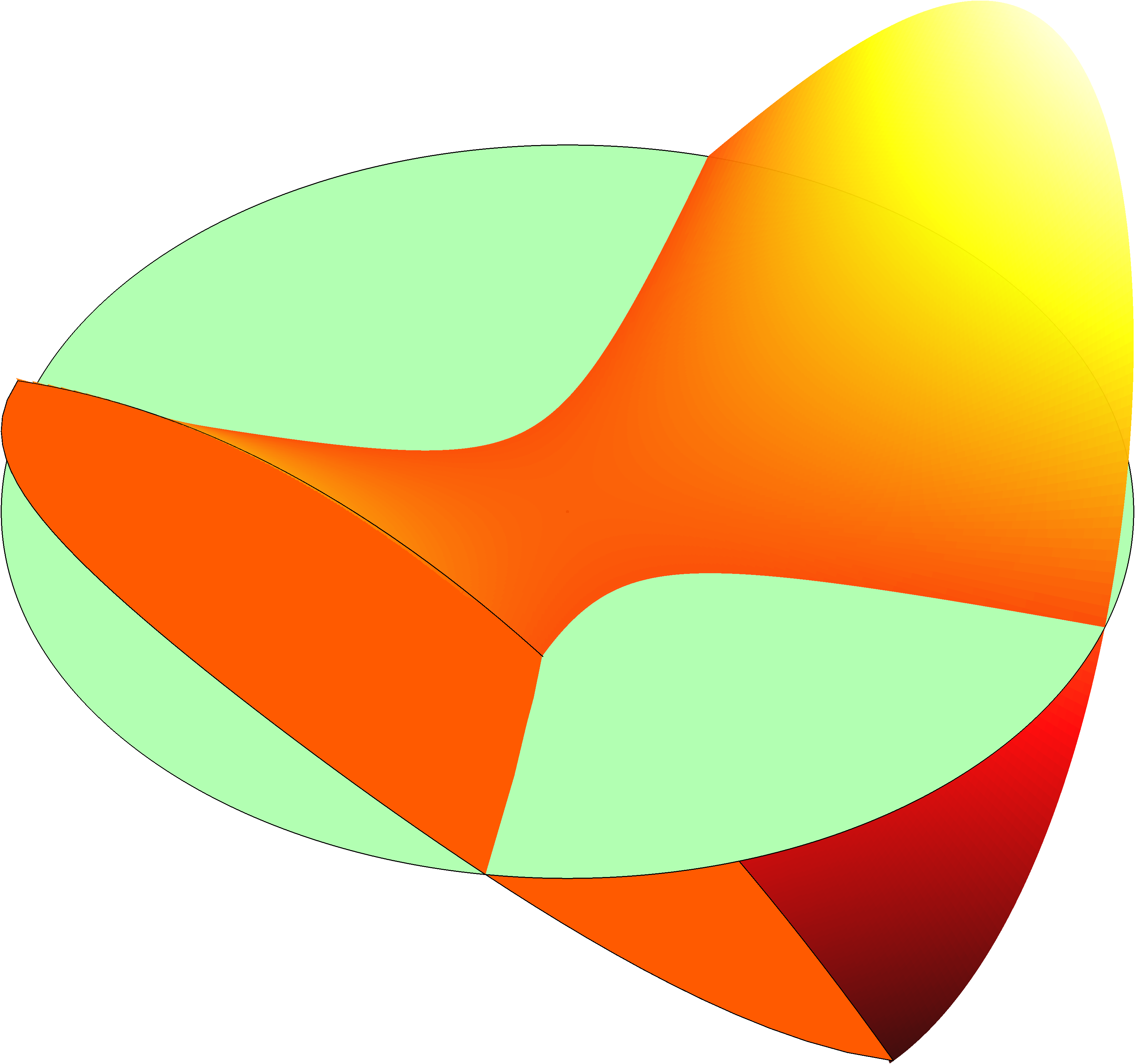
Thus, to ensure that we will need at least number of polytopes in our construction, and the size of the resulting -band of over scales as . The sequence of polytopes for a given is depicted in Figure 18 together with the resulting -band. Proposition 4.3 shows that we can construct a network such that the graph is mapped in a controlled way and that the size of the -band can be made arbitrarily small by choosing sufficiently small. Before turning to what the implications are for the decision boundary with respect to our construction, we will first estimate the total number of layers needed in the realization of the network we have described.
4.4 Total Number of Layers
Recall that the total number of layers is equal to the sum in (4.38). Previously, we derived the bound in Lemma 4.9 on the number of polytopes which equals the number of maps in (4.36). In each map we have layers and in our construction we defined as the cardinality of an -net of the sphere .
Separations.
To prove Lemma 4.7, we defined . Thus, to give a bound on the number of layers needed in our construction we will need to estimate the cardinality of an -net of a sphere. We begin by defining the related concept of an -separation.
Definition 4.2 (-separation).
Given a set we say that a subset is an -separation of if for any distinct pair of points we have that . If in addition there is no superset which is also an -separation of , we say that is a maximal -separation of .
A standard way of estimating the cardinality of -nets is to give a bound on maximal -separations and then apply the following Lemma.
Lemma 4.10.
A maximal -separation of a set is also an -net of .
-
Proof.Let be a maximal -separation of . Suppose there is a point such that for all . Then would still be an -separation of contradicting the maximality of . Thus, there can’t exist such a point , and hence is an -net of . ∎
We will now give a bound on in case is an -net of a sphere of radius .
Lemma 4.11.
There is an -net of the sphere such that .
In the proof, outlined in Appendix A.2, we use the relation between -nets and -separations presented in Lemma 4.10. Using Lemma 4.11 we can now give a bound on the number of layers needed in our construction.
Proposition 4.4 (Number of Layers).
The total number of layers in our construction satisfies
| (4.78) |
for a constant independent of , , and .
5 Decision Boundary
We can express the decision boundary in terms of our canonical network architecture (3.15) as
| (5.1) |
where each
| (5.2) |
and denotes the preimage of a set under layer .
Defining the Affine Function.
Up to now we have described the construction of each layer in our network but the last affine function . We will now show that we can choose the hyperplane
| (5.3) |
so that its restriction to , denoted by , is contained in the -band of over for the same value of as in Proposition 4.3, see Figure 19. Since the graph of an affine function in -variables is a hyperplane in we can choose
| (5.4) |
for the affine function given by
| (5.5) |
As we have by Taylor’s theorem that
| (5.6) |
for any and where . Hence,
| (5.7) |
for all . Since it follows that so we get the upper bound
| (5.8) |
Hence, we can write
| (5.9) |
Recalling the value of in Proposition 4.3 and since (see the proof of Proposition 4.1 in Appendix A.2) it follows that
| (5.10) |
Thus, we have
| (5.11) |
Preimages.
By construction, a point in the domain of the network with will be mapped into the set by the composition . Thus, any point with will have an empty preimage under this composition. Therefore, we can express the decision boundary as the preimage of just as this is exactly the part of the hyperplane with a nonempty preimage. Then, by the inclusion in (5.11) we have that
| (5.12) |
for the value of given in Proposition 4.3. As each is a composition of several layers we will need to understand their preimages as these are the building blocks in our network.
Lemma 5.1 (Preimages).
Let be a continuous function and denote its graph by . Consider a layer in our network . Then, the preimage of under fulfills
| (5.13) |
where is the graph of a continuous function . Moreover, given any we have
| (5.14) |
The details of the proof can be found in Appendix A.3. The idea is that the preimage of the intersection of the graph and the hyperplane associated to a layer is spanned by a constant vector, the negative projection direction for that layer. The part of the graph contained in the halfspace will just be its own preimage as the layer is the identity when restricted to this set. This is illustrated in Figure 20.
Decision Boundary.
Using Lemma (5.1) we can prove that the decision boundary is the graph of a continuous piecewise linear function.
Corollary 5.1.
There is a continuous piecewise linear function with graph such that .
-
Proof.From (5.1) and (5.2) we see that is the preimage of the hyperplane under a sequence of layers . Recall equation (5.4) where we defined as the graph of the affine function . Thus, taking the preimage of by a layer will generate a graph of a new continuous function by Lemma 5.1. In particular, it follows from the proof of Lemma 5.1 that the preimage of the graph of a piecewise linear function under a layer will be the graph to a piecewise linear function. Hence, by repeatedly applying this lemma, for all layers in the network, we will get a piecewise linear continuous function such that its graph coincides with the decision boundary . ∎
This corollary guarantees that the decision boundary of our network can be represented as the graph of a piecewise linear continuous function defined on . Therefore, we will hereafter denote the decision boundary by where is the function which existence is established by the corollary above. We choose to denote this function by as it will be a piecewise linear approximation of . To prove the main result of this paper the following proposition will be useful.
Proposition 5.1.
There is a continuous function such that
| (5.17) |
where .
-
Proof.First, we make the observation that
(5.18) as the preimage of the set is empty since the image of the domain under this composition is contained in . Thus, from equation (5.12) we have the inclusion
(5.19) with . Now, we define to be the function whose graph is given by
(5.20) Note that the preimage on the right-hand side above is guaranteed to generate a graph of a continuous function on by repeatedly applying the first part of Lemma 5.1 to each layer in the composition. Similarly, applying the second part of Lemma 5.1 repeatedly we get
(5.21) Combining the inclusion in (5.19) and equation (5.21) gives
(5.22) which we wanted. To prove the second inclusion we first note that by Proposition 4.3 we know
(5.23) for the given . But as it is also true that
(5.24) Thus, in particular
(5.25) and hence
(5.26) by (5.21). ∎
We are now ready to state and prove the main result of this paper.
Theorem 5.1 (Error Estimate).
Let be a -function with bounded second-order partial derivatives. For each positive , we can construct a fully-connected ReLU network of width and depth at most , for a constant , such that the decision boundary of can be represented as the graph of a continuous piecewise linear function satisfying
| (5.27) |
where is a constant independent on and .
-
Proof of Theorem 5.1.Let be the function in Proposition 5.1. As noted in Remark 2.2, it follows that
(5.28) for . By the triangle inequality we get
(5.29) Plugging in the value of in (5.29) gives
(5.30) where . The bound on the number of layers follows from Proposition 4.4. As our modified network architecture can be rewritten as a standard fully-connected ReLU network, by Lemma 3.1, the theorem follows. ∎
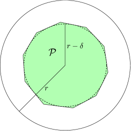
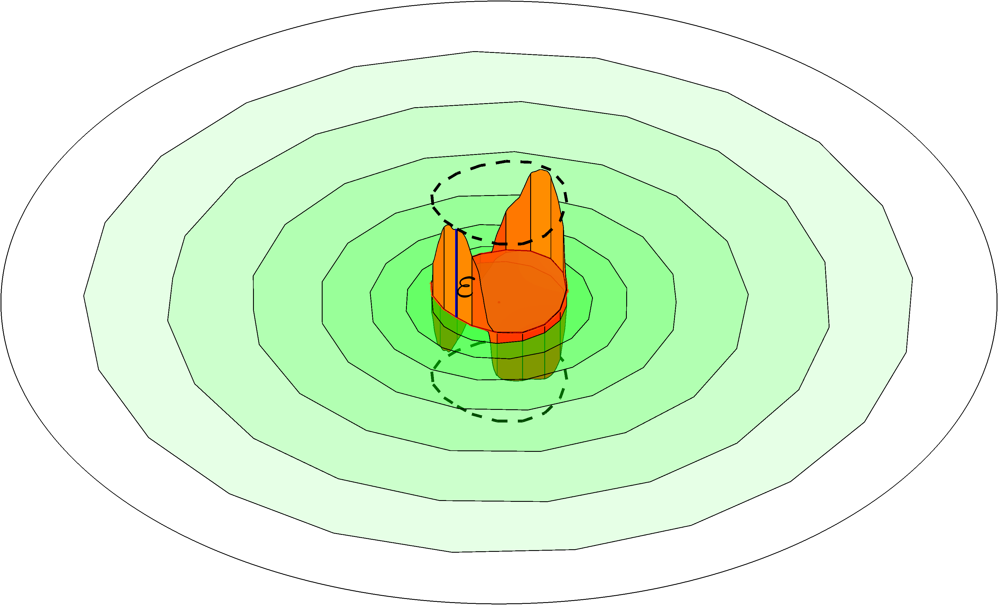
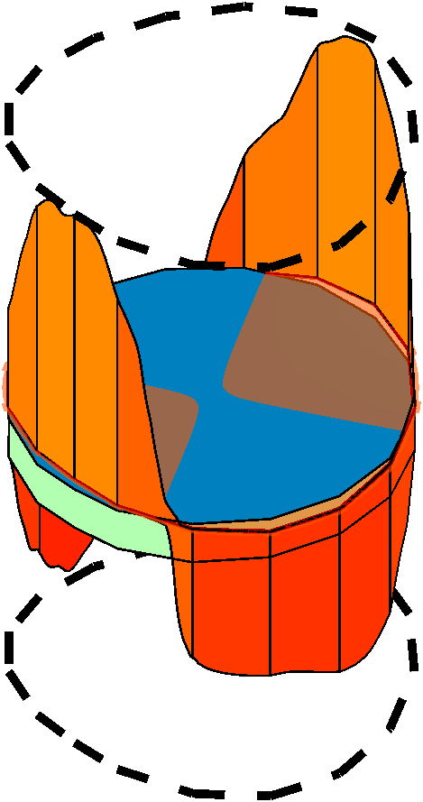
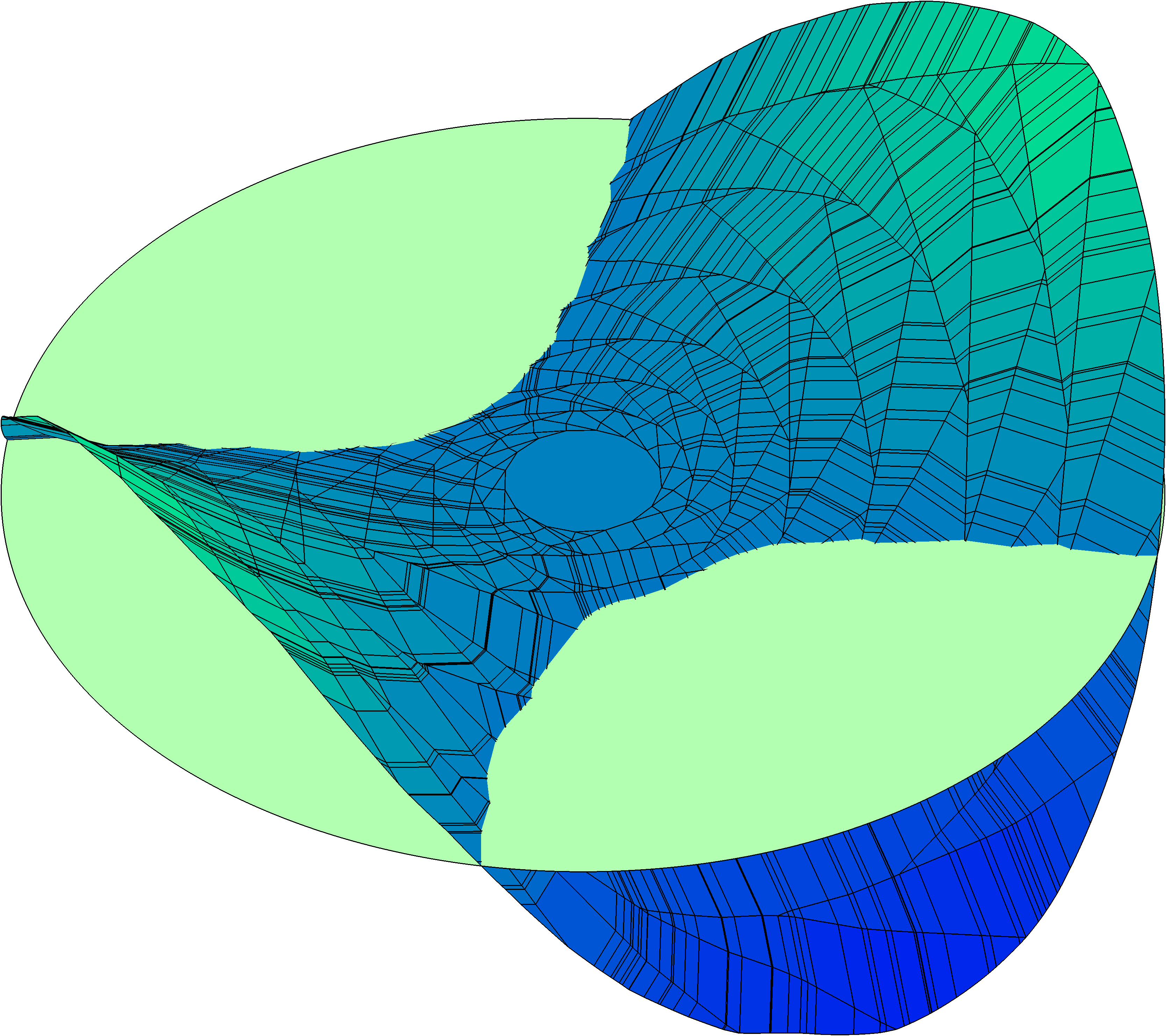
An example of the resulting decision boundary generated by the sequence of polytopes in Figure 18 is shown in Figure 21. By choosing small enough we can approximate to any accuracy.
Corollary 5.2.
Given there is a fully-connected ReLU network of width and depth at most , for a constant , such that the corresponding function -approximates
| (5.31) |
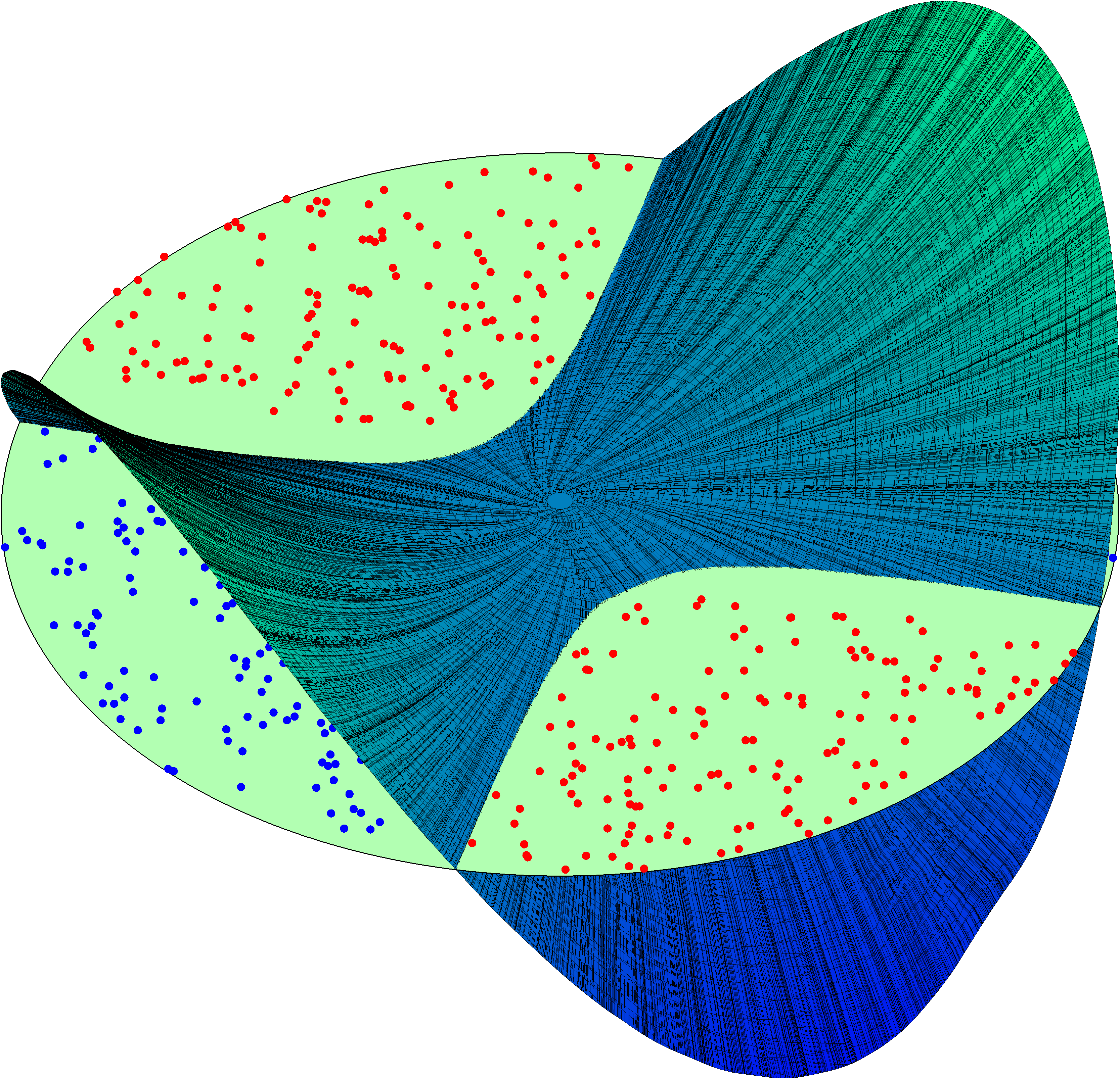
Remark 5.1 (Proof of Lemma 2.1).
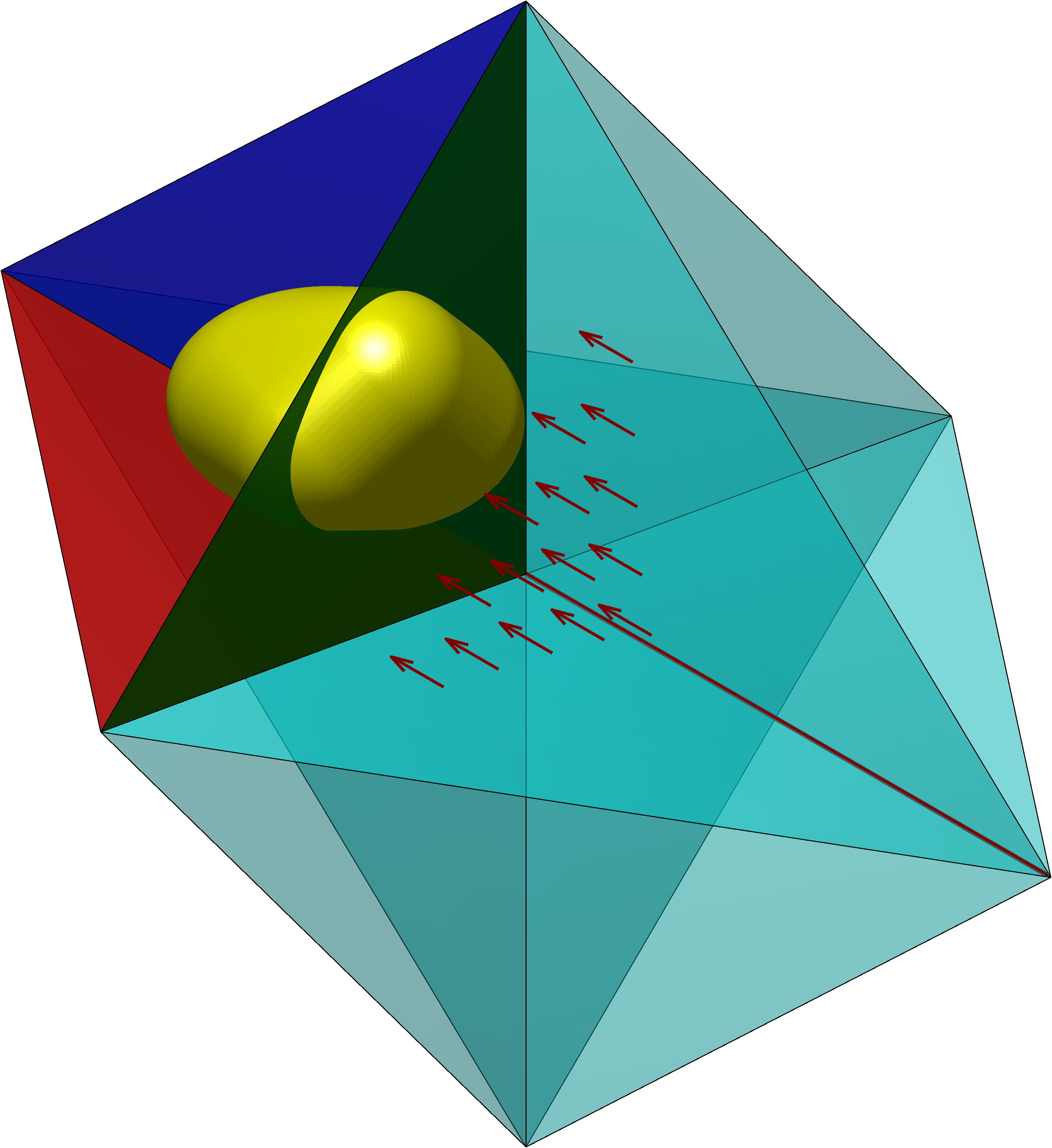
Figure 22 shows a finer approximation to (using a smaller value of ) and the corresponding decision boundary when restricting to , i.e., the network’s approximation to .
6 Conclusions
We have developed an approximation theory for deep fully-connected ReLU networks. Based on the geometrical description of ReLU layers we proposed a modified network architecture. Each such network can explicitly be rewritten as a standard fully-connected ReLU network. A key observation was how these layers could be reduced to projections on hyperplanes along given directions.
Our result shows that if there exists a hypersurface separating two classes of points in a binary classification problem, then the decision boundary of a fully-connected ReLU network can approximate this surface to any given accuracy as long as it can be represented as a level-set of a -function . Our proof is constructive and we have derived an explicit upper bound on the approximation error in terms of the discretization parameter , input dimension , level-set function and radius of the domain . We have described in detail how the graph is mapped when propagating through the layers in the network and how the decision boundary emerges as the preimage of a hyperplane identified as the kernel of the final affine layer.
To achieve a given approximation error our construction requires layers. This estimate is in line with the related work[11], and the exponent seems unavoidable without any further assumption on the level-set function .
Apart from the rich expressiveness of the class of functions defined by a network architecture, the success of deep learning also stems from the fact that these networks can be trained properly in practice. This is often done by using some variant of the stochastic gradient descent (SGD) algorithm [8, 14] to solve an optimization problem. One key aspect that might partly explain why these learning algorithms are able to find feasible solutions could be that there are many different values of the network parameters that are sufficiently good for the problem at hand.
In line with this, we discussed in Section 3.1 that many different affine maps generate the same cone and many cones can be reduced to the same projections in our construction. Further, the order of the layers in each map does not matter and the exact placement of the hyperplanes in the layers is not very important as long as they cover the ball in the -net sense. In our proof, we explicitly defined the projection directions as the directional derivative of at a given point to obtain a good approximation accuracy. But as noted in Remark 2.4, in classification problems high accuracy is only essential in regions where the two sets of data are close to each other. Therefore, one may conclude that the choice of projection directions can be less restrictive on other parts of the domain. Similarly, if there are many possible separating hypersurfaces (recall Figure 4) it is enough to find a set of network parameters realizing an approximation of one of them.
On the other hand, from the geometrical description provided in Section 2 it is clear that the layers cannot be chosen without any caution. If points from different classes are mapped to the same point it will not be possible to obtain a separating decision boundary. For instance, imagine if the cone of the first layer is positioned in the center of a point cloud of the data. Then there would be a high risk that the data gets mixed when it is projected onto the cone boundary. Especially in parts of the induced partition which are mapped to low-dimensional faces. Therefore, it seems reasonable to start projecting small parts from the boundary of the domain inwards towards the center as in the proposed construction in this paper.
Acknowledgement.
This research was supported in part by the Wallenberg AI, Autonomous Systems and Software Program (WASP) funded by the Knut and Alice Wallenberg Foundation; the Swedish Research Council Grants Nos. 2017-03911, 2021-04925; and the Swedish Research Programme Essence.
References
- [1] M. Alfarra, A. Bibi, H. Hammoud, M. Gaafar, and B. Ghanem. On the decision boundaries of neural networks: A tropical geometry perspective. IEEE Trans. Pattern Anal. Mach. Intell., 45(4):5027–5037, 2022. doi:10.1109/TPAMI.2022.3201490.
- [2] J. Ba and R. Caruana. Do deep nets really need to be deep? In Proceedings of the 28th International Conference on Neural Information Processing Systems (NIPS’14), volume 27 of Adv. Neural Inf. Process. Syst., 2014. doi:10.48550/arXiv.1312.6184.
- [3] H.-P. Beise, S. Dias Da Cruz, and U. Schröder. On decision regions of narrow deep neural networks. Neural Networks, 140:121–129, 2021. doi:10.1016/j.neunet.2021.02.024.
- [4] A. Berzins. Polyhedral complex extraction from relu networks using edge subdivision. In International Conference on Machine Learning, pages 2234–2244. PMLR, 2023.
- [5] T. B. Brown et al. Language models are few-shot learners. In Proceedings of the 34th International Conference on Neural Information Processing Systems (NeurIPS’20), volume 33 of Adv. Neural Inf. Process. Syst., 2020. doi:10.48550/arXiv.2005.14165.
- [6] S. Bubeck et al. Sparks of artificial general intelligence: Early experiments with gpt-4. arXiv preprint arXiv:2303.12712, 2023.
- [7] G. Cybenko. Approximation by superpositions of a sigmoidal function. Math. Control Signals Syst., 2(4):303–314, 1989. doi:10.1007/BF02551274.
- [8] J. Duchi, E. Hazan, and Y. Singer. Adaptive subgradient methods for online learning and stochastic optimization. Journal of machine learning research, 12(7), 2011.
- [9] A. Fawzi, S.-M. Moosavi-Dezfooli, P. Frossard, and S. Soatto. Empirical study of the topology and geometry of deep networks. In Proceedings of the IEEE/CVF Conference on Computer Vision and Pattern Recognition, pages 3762–3770, 2018. doi:10.1109/CVPR.2018.00396.
- [10] B. Hanin and D. Rolnick. Deep ReLU networks have surprisingly few activation patterns. In Proceedings of the 33rd International Conference on Neural Information Processing Systems (NeurIPS’19), volume 32 of Adv. Neural Inf. Process. Syst., 2019. doi:10.48550/arXiv.1906.00904.
- [11] B. Hanin and M. Sellke. Approximating continuous functions by ReLU nets of minimal width. arXiv:1710.11278, 2017. doi:10.48550/arXiv.1710.11278.
- [12] K. He, X. Zhang, S. Ren, and J. Sun. Deep residual learning for image recognition. In Proceedings of the 2016 IEEE Conference on Computer Vision and Pattern Recognition (CVPR), pages 770–778, 2016. doi:10.1109/CVPR.2016.90.
- [13] J. Huchette, G. Muñoz, T. Serra, and C. Tsay. When deep learning meets polyhedral theory: A survey. arXiv preprint arXiv:2305.00241, 2023.
- [14] D. P. Kingma and J. Ba. Adam: A method for stochastic optimization. arXiv preprint arXiv:1412.6980, 2014.
- [15] A. Krizhevsky, I. Sutskever, and G. E. Hinton. ImageNet classification with deep convolutional neural networks. Commun. ACM, 60(6):84–90, may 2017. doi:10.1145/3065386.
- [16] S. Lee, A. Mammadov, and J. C. Ye. Defining neural network architecture through polytope structures of dataset. arXiv preprint arXiv:2402.02407, 2024.
- [17] B. Liu and M. Shen. Some geometrical and topological properties of DNNs’ decision boundaries. Theor. Comput. Sci., 908:64–75, 2022. doi:10.1016/j.tcs.2021.11.013.
- [18] Z. Lu, H. Pu, F. Wang, Z. Hu, and L. Wang. The expressive power of neural networks: A view from the width. In Proceedings of the 31st International Conference on Neural Information Processing Systems (NIPS’17), volume 30 of Adv. Neural Inf. Process. Syst., 2017. doi:10.48550/arXiv.1709.02540.
- [19] G. Montúfar, R. Pascanu, K. Cho, and Y. Bengio. On the number of linear regions of deep neural networks. In Proceedings of the 27th International Conference on Neural Information Processing Systems (NIPS’14), volume 26 of Adv. Neural Inf. Process. Syst., 2014. doi:10.48550/arXiv.1402.1869.
- [20] S.-M. Moosavi-Dezfooli, A. Fawzi, J. Uesato, and P. Frossard. Robustness via curvature regularization, and vice versa. In Proceedings of the IEEE/CVF Conference on Computer Vision and Pattern Recognition, pages 9078–9086, 2019. doi:10.1109/CVPR.2019.00929.
- [21] Q. Nguyen, M. C. Mukkamala, and M. Hein. Neural networks should be wide enough to learn disconnected decision regions. In Proceedings of the 35th International Conference on Machine Learning, volume 80 of Proc. Mach. Learn. Res., pages 3740–3749, 2018. https://proceedings.mlr.press/v80/nguyen18b.html.
- [22] S. Park, C. Yun, J. Lee, and J. Shin. Minimum width for universal approximation. In International Conference on Learning Representations, 2021. https://openreview.net/forum?id=O-XJwyoIF-k.
- [23] P. Piwek, A. Klukowski, and T. Hu. Exact count of boundary pieces of relu classifiers: Towards the proper complexity measure for classification. In Uncertainty in Artificial Intelligence, pages 1673–1683. PMLR, 2023.
- [24] P. P. Ray. Chatgpt: A comprehensive review on background, applications, key challenges, bias, ethics, limitations and future scope. Internet of Things and Cyber-Physical Systems, 3:121–154, 2023.
- [25] D. Silver et al. Mastering the game of Go without human knowledge. Nature, 550(7676):354–359, 2017. doi:10.1038/nature24270.
- [26] M. Telgarsky. Representation benefits of deep feedforward networks. arXiv:1509.08101, 2015. doi:10.48550/arXiv.1509.08101.
- [27] M. Telgarsky. Benefits of depth in neural networks. In 29th Annual Conference on Learning Theory, volume 49 of Proc. Mach. Learn. Res., pages 1517–1539, 2016. https://proceedings.mlr.press/v49/telgarsky16.html.
- [28] J. Vallin, K. Larsson, and M. G. Larson. The geometric structure of fully-connected ReLU-layers. arXiv:2310.03482, 2023. doi:10.48550/arXiv.2310.03482.
- [29] A. Vaswani et al. Attention is all you need. In Proceedings of the 31st International Conference on Neural Information Processing Systems (NIPS’17), volume 30 of Adv. Neural Inf. Process. Syst., 2017. doi:10.48550/arXiv.1706.03762.
- [30] Y. Wu et al. Google’s neural machine translation system: Bridging the gap between human and machine translation. CoRR, abs/1609.08144, 2016. doi:10.48550/arXiv.1609.08144.
- [31] D. Yarotsky. Error bounds for approximations with deep ReLU networks. Neural Networks, 94:103–114, 2017. doi:10.1016/j.neunet.2017.07.002.
- [32] L. Zhang, G. Naitzat, and L.-H. Lim. Tropical geometry of deep neural networks. In Proceedings of the 35th International Conference on Machine Learning, volume 80 of Proc. Mach. Learn. Res., pages 5824–5832, 2018. https://proceedings.mlr.press/v80/zhang18i.html.
Authors’ addresses:
Jonatan Vallin Mathematics and Mathematical Statistics, Umeå University, Sweden
jonatan.vallin@umu.se
Karl Larsson, Mathematics and Mathematical Statistics, Umeå University, Sweden
karl.larsson@umu.se
Mats G. Larson, Mathematics and Mathematical Statistics, Umeå University, Sweden
mats.larson@umu.se
Appendix A Proofs
In this appendix, we present the proofs of auxiliary lemmas and propositions that were omitted from the main text.
A.1 Proofs of Section 3
Lemma 3.2 (Projections on Hyperplanes).
Let be a bounded set. Given a closed half-space with the hyperplane as its boundary and a vector not parallel to , we can construct a projection defined as in (3.9) such that projects on along while acting as the identity on .
-
Proof.The action of on will depend on the corresponding cone and its intersection with . As noted before, the cone can be derived given an affine map and conversely. We will show how to construct a matrix and a vector such that the affine map generates a cone for which the corresponding projection satisfies the conditions. Fix an index and define the :th row vector in and the :th scalar in such that coincides with the given half-space . Then, we decompose the set into and .
We want to show that we can choose the other row vectors and the vector components for such that realizes a map projecting on the hyperplane along the given direction while leaving unchanged. We continue by defining a set of linearly independent vectors , , in such that the line
(A.1) is parallel to the given direction . The dual vector is thus parallel to . Then, we can choose , , such that
(A.2) where each is the interior of the corresponding closed half-space defined in (3.11). Note that this is always possible since is a bounded set in and therefore we can translate each open half-space in (A.2), by tuning , until .
With this set of parameters, the matrix will have full rank since the linearly independent vectors are all orthogonal to (by construction) which in turn is not orthogonal to (since is, by assumption, not parallel to the hyperplane with normal ). Thus, with these parameters we will get a cone such that
(A.3) Then, according to equation (3.9) the corresponding projection will act as the identity on whereas will be projected along onto the hyperplane . The construction is depicted in Figure 7. ∎
Remark A.1.
The vectors , in the proof are not uniquely determined as the only requirements are that they are linearly independent and that the line in (A.1) is parallel to the given vector . In the same way, there are many different values of the scalars , yielding the same action on by . The condition in (A.2) is met as long as we choose the scalars such that all the corresponding open half-spaces , contain . Thus, moving these half-spaces such that their corresponding hyperplanes are even further away from will not change how is mapped by .
A.2 Proofs of Section 4
-
Proof.We first introduce a new local coordinate system of situated at the center point of the base of the spherical cap. We name the corresponding new variables . Let the coordinate axis for the first coordinate be defined along the negative -direction, i.e., in the direction pointing out from the half-space . The other coordinate axes can then be chosen arbitrarily as long as the resulting coordinate system is orthogonal. Thus, the coordinate axes meet at the center and lie in the hyperplane . Figure 23 illustrates the construction of the local coordinate system.
(a) 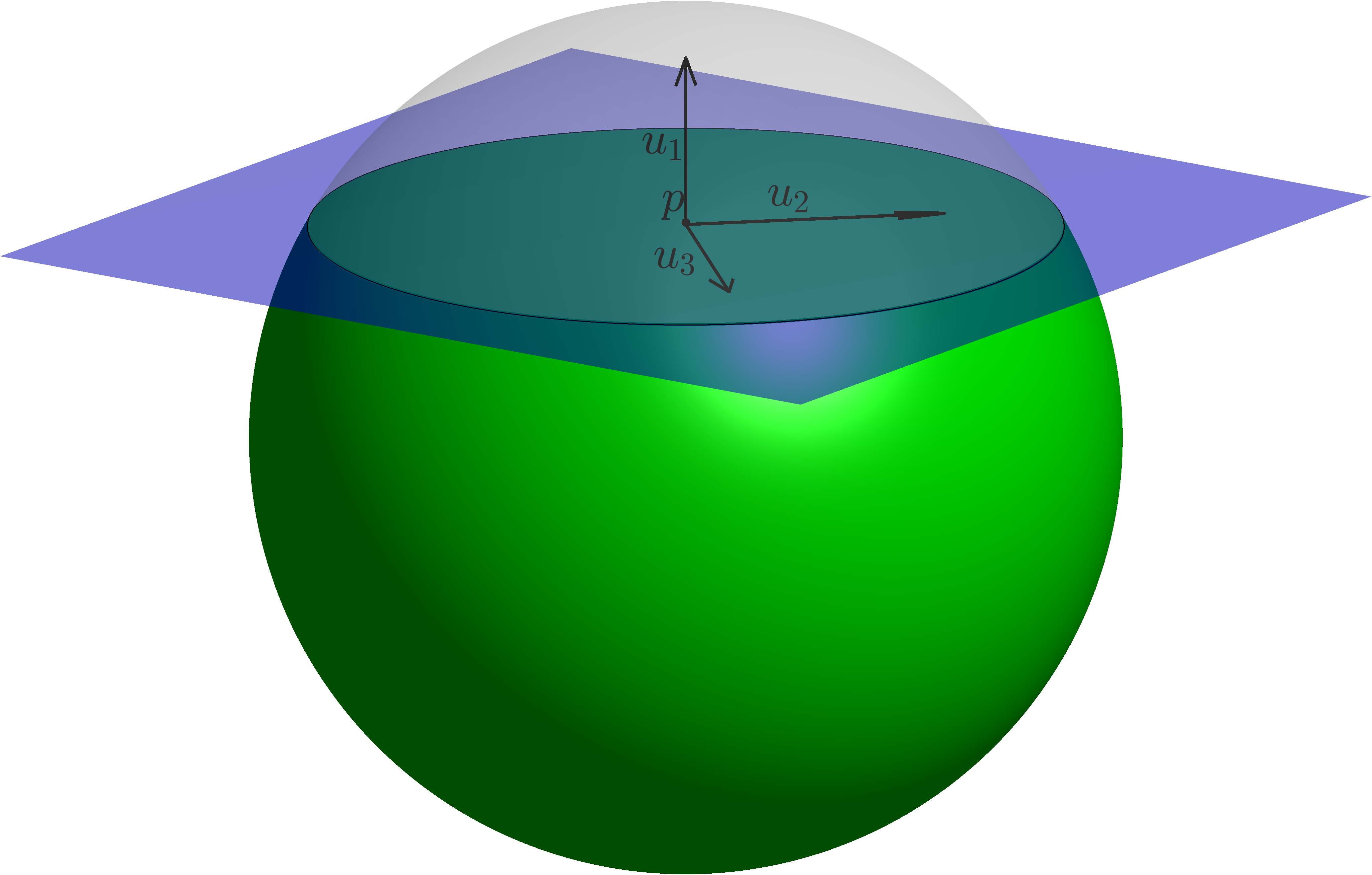
(b) Figure 23: Local Coordinate System. The construction of the new coordinate system in case (a) and (b) . The first coordinate axis is defined along the negative -direction whereas the other coordinate axes are parallel to the hyperplane . The new axes meet at the center point . We note that the origin in this coordinate system coincides with the point and if we let denote the function expressed in the new coordinates we see that . Since , the point expressed in the new coordinate system will have coordinates for some satisfying
(A.4) as the point lies inside the spherical cap (see Figure 11). Similarly, as lie in and points in the negative direction, this point will have coordinates . We can now express the quantity in (4.6) in terms of the new variables
(A.5) By Taylor’s theorem we can write
(A.6) for some . Similarly, expanding in the expression above as a Taylor polynomial in the variables with a first order remainder term gives
(A.7) for some . Combining (A.6) and (A.7) we get
(A.8) Using this in equation (A.5) we obtain
(A.9) where we used that and assumed that in the last inequality. Recall that is the constant bounding the second order derivatives of . Thus,
(A.10) where . ∎
Remark A.2.
If , then from the second last inequality in (A.9) and the argument in the proof of the Corollary 4.1 shows that scales as which is more favorable than as we get in the higher-dimensional cases. This is because if , the size of the piece we cut off by the half-space only scales as since we do not have any of the additional directions perpendicular to that introduced a factor of into our estimate.
-
Proof.Note, from (4.13) we have that and intersect in if and only if the minimizer to the constrained optimization problem
(A.11) satisfies . To find the minimizer of problem (A.11) we construct the Lagrangian
(A.12) with . Then, by solving the linear system
(A.13) we get the minimizer with squared norm . Setting and solving for yields (4.20). ∎
Lemma 4.3.
-
Proof.From (4.4) we have
(A.14) Rewriting the first two terms in the same way and then repeating the procedure -times gives us
(A.15) where we used that by (4.15). By the triangle inequality we then have
(A.16) Note that each term for which vanishes since then by (4.17). If then and hence, we can apply Proposition 4.1. Thus, we can bound each term by
(A.17) We can now bound the sum as
(A.18) as desired. ∎
-
Proof.If the inequality follows trivially, so assume that . We start by deriving an expression of in terms of and . Note that all the points , and lie in the 2-dimensional plane spanned by and the vector pointing from to . Figure 24 illustrates the geometrical setup in this plane.
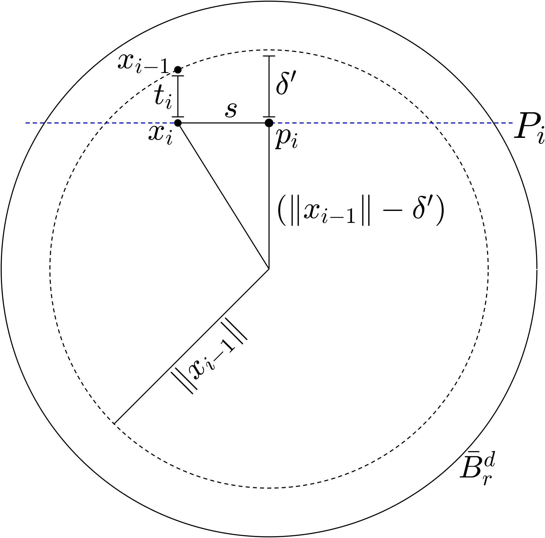
Figure 24: Geometrical Setup. The origin, the point and define a right triangle where the length of the hypotenuse is . Calculating the side length allows us to compute . Let be the height of the spherical cap as depicted in the figure, then since is the height of the spherical cap it follows that
(A.19) Now, consider the right triangle in this plane with vertices at the origin, and . The hypotenuse has length which we are interested in and the side from the origin to has length . We denote by , the length of the third side between and , and the Pythagorean theorem gives the relation
(A.20) We can calculate the side length by considering the spherical cap resulting from translating the hyperplane a distance such that it passes through . Then, the radius of its base is precisely . Since the height of the new spherical cap is we get that
(A.21) Plugging this into (A.20) gives
(A.22) Using the relation in (A.19) in the equation above yields
(A.23) and thus
(A.24) which we wanted to show.
In case lies on the line passing through the origin and , then the triangle described above is degenerate as . However, in this case we have the equality and thus
(A.25) where the last inequality follows from the fact that neither of and are contained in . Hence, the inequality also holds in this special case. ∎
-
Proof.The first inclusion holds trivially by the construction of , recall (4.43). To prove the second inclusion we will show that because then but since is connected and contains the origin, the last inclusion implies that .
Let be an -net of . Take a point , then there is a point such that . With we thus have . By the definition of , we have that is a spherical cap of height and the radius of the base is precisely . As is the point on the top of this spherical cap, and thus a distance from , it follows from the Pythagorean theorem that
(A.26) Thus, as we must have . Hence, so . ∎
Lemma 4.9 (Number of Polytopes).
The number of polytopes needed in our construction to ensure satisfies
| (4.71) |
-
Proof.Recall that is either set to or the value depending on the relative size of and , see equation (4.44). Now, if we define
(A.27) then as long as . We can also express
(A.28) where represent the number of polytopes in our construction for which and represent the number of polytopes for which .
Note, for all with we have by Lemma 4.7 that . Solving the equation for gives . Thus we can write
(A.29) where is the ceiling function. We can now estimate by considering how many polytopes we need in our construction to go from the radius to . In this case we have that so by Lemma 4.7
(A.30) If is the first index such that then for any we get
(A.31) Solving gives so we get
(A.32) Combining (A.29) and (A.32) in (A.28) gives the bound
(A.33) where the last inequality holds since . ∎
Lemma 4.11.
There is an -net of the sphere such that .
-
Proof.Let be a maximal -separation of . Since it is an -separation, the balls are disjoint. Moreover, the disjoint union is contained in the spherical shell . By comparing volumes we get the inequality
(A.34) where denotes the volume of a dimensional ball of radius . Now, we can estimate the right-hand side (assuming )
(A.35) Dividing by gives the upper bound
(A.36) The result now follows from Lemma 4.10. ∎
A.3 Proofs of Section 5
Lemma 5.1 (Preimages).
-
Proof.To simplify the notation we will drop the sub- and superscript on the layer and simply denote it by . Let be the closed half-space, associated with the layer, with boundary hyperplane and inward pointing unit normal . Further let be the projection direction and let be the point such that . Then it follows that
(A.37) as act as the identity on the interior and any point in will be mapped to disjoint with . Therefore, the only part of with a non empty and a non trivial preimage is precisely .
For a point , we have that . From (4.4) we can then immediately see that a point will be mapped to if and only if
(A.38) for some . Therefore, we can express the preimage of this point as
(A.39) and the entire preimage of can be written as
(A.40) Fixing in the set builder above we see that, in particular,
(A.41) Further, as we will have that . This suggests that we can define the function by
(A.42) where and are defined by the equation . However, we must show that for all we can find such a point and non-negative scalar and that they are unique so the function is well-defined.
Given a point , we can define the unique hyperplane parallel to such that . Then we let dist and we define to be the orthogonal projection of onto . Clearly, but as we also know that contains the origin (this is true for the associated half-spaces to all the layers in our construction) the ball has smaller or equal radius than the parallel ball and hence we have that . Then, by construction we have .
To show the uniqueness, suppose
(A.43) for and . We can rewrite the equation as
(A.44) As both the points are contained in , the vector on the left-hand side in (A.44) is perpendicular to the vector on the right-hand side. Thus, for the equality to hold we need both sides to vanish meaning that and . Hence, we can conclude that defined in (A.42) is a valid and well-defined function.
| (A.46) |
The preimage of the graph of under such a layer is shown in Figure 20.
To prove the second part of the lemma, suppose and consider the set . Similarly as before, we have that
| (A.47) |
where the second equality follows from the fact that on . Thus, the only part with non empty and non trivial preimage is exactly . Therefore, consider a point . Then by definition of preimages we have that . By definition of we need and with . Using equation (4.4) we therefore need
| (A.48) | ||||
for some . But so . If we similarly consider a point we have that and with . As we can express it as for some and . Thus, .