Nonlocal-to-local convergence of the Cahn-Hilliard equation with degenerate mobility and the Flory-Huggins potential.
Abstract
The Cahn-Hilliard equation is a fundamental model for phase separation phenomena. Its rigorous derivation from the nonlocal aggregation equation, motivated by the desire to link interacting particle systems and continuous descriptions, has received much attention in recent years. In the recent article, we showed how to treat the case of degenerate mobility for the first time. Here, we discuss how to adapt the exploited tools to the case of the mobility as in the original works of Giacomin-Lebowitz and Elliott-Garcke. The main additional information is the boundedness of , implied by the form of mobility, which allows handling the nonlinear terms. We also discuss the case of (mildly) singular kernels and a model of cell-cell adhesion with the same mobility.
2010 Mathematics Subject Classification. 35B40, 35D30, 35K25, 35K55.
Keywords and phrases. degenerate Cahn-Hilliard equation; nonlocal Cahn-Hilliard
equation; aggregation-diffusion; singular limit; cell-cell adhesion.
1 Introduction
The question of nonlocal-to-local convergence for the Cahn-Hilliard equation is of fundamental nature, linking the models derived from particle processes or interacting particle systems [40] and from physical principles [7, 8]. This question was recently addressed by several authors [20, 18, 50, 19] but only for the case of constant mobility. Our recent article [25] was the first one to establish rigorously the convergence for the degenerate mobility and smooth potential as a consequence of nonlocal compactness results developed by Bourgain-Brezis-Mironcescu [3] and Ponce [55]. In the current paper we conclude our analysis by showing that the reasoning from [25] can be extended to the mobility and the logarithmic Flory-Huggins potential as in the original works of Giacomin-Lebowitz [40] and Elliot-Garcke [27]. We also consider singular nonlocal interaction kernels in the spirit of [20]. In the last section, using similar techniques, we also discuss the nonlocal-to-local limit of a model of cell-cell adhesion with the same mobility introduced in [13].
We consider the nonlocal Cahn-Hilliard equation with degenerate mobility
| (1.1) |
equipped with an initial datum . Here, the mobility is , is the -dimensional flat torus, which is particularly useful when treating nonlocal operators, is the nonlocal operator defined with
| (1.2) |
The convolution kernel is of the form
| (1.3) |
for , where is the family of standard mollifiers:
| (1.4) |
with being a nonnegative smooth radially symmetric kernel which is compactly supported in the unit ball of satisfying
| (1.5) |
for some .
Remark 1.1.
The range ensures that the kernel is in and therefore we can apply the existing theory of the existence of weak solutions for the nonlocal equation. This type of kernel has for instance been considered in [19].
The potential is the usual double-well logarithmic potential
| (1.6) |
where and is a constant such that for all . Note in particular the identities
| (1.7) |
We impose the constraint on the parameter
| (1.8) |
for some . This is always satisfied for small enough since
As we intend to send , we can assume that this condition is always satisfied. The condition (1.8) ensures that the coefficient (standing next to in (1.1)) is strictly positive and the existence as well as uniqueness of the weak solution follows.
Our target is to prove that as , the solutions of
| (1.9) | ||||
| (1.10) |
tend to the weak solution of the degenerate Cahn-Hilliard equation
| (1.11) | ||||
| (1.12) |
Our main result reads as follows.
Theorem 1.2 (Convergence of nonlocal to local Cahn-Hilliard equation on the torus).
Let be an initial datum with finite energy and entropy defined in (3.1) and (3.2). Let , with defined in Lemmas C.1-C.3, be a sequence of solutions of the nonlocal Cahn-Hilliard equation (1.9)-(1.10) as in Proposition 3.1. Then, along a subsequence not relabeled,
where is a weak solution of the degenerate Cahn-Hilliard equation (1.11)-(1.12) as defined in Definition 4.1.
Remark 1.3.
If , then , see [3, Theorem 1].
The main contribution of Theorem 1.2 is the possibility to consider more general, nonlinear mobilities . In [25], where we considered the particular mobility , we exploited the formula
in a crucial way. This is no longer available when . However, the more general term can be still handled because the singular Flory-Huggings potential ensures that the sequence is uniformly bounded in .
We also would like to point out that while the setting above is formulated for the standard choice , the same is also true for more general case where . In particular, the proof of Theorem 1.2 and of the crucial Lemma 4.5, is formulated in so general way that it uses only the fact that is a function.
The structure of the paper is as follows. In Section 2 we review the existing literature on the problem while in Section 3 we recall the basic properties of the system (1.9)-(1.10) (well-posedness, energy, and entropy estimates). Section 4 is dedicated to the proof of the main results. In Section 5 we present numerical simulations which show certain qualitative differences between the local and nonlocal models. The last section, Section 6, is devoted to a model of cell-cell adhesion phenomena from [13], which also includes the mobility . For this model we also obtain a nonlocal-to-local convergence result.
2 Motivations and litterature review
The non-local Cahn-Hilliard equation was initially derived by Giacomin and Lebowitz [40, 41] through a microscopic approach. Their model is based on a -dimensional lattice gas that evolves through Kawasaki exchange dynamics, which is a Poisson process that exchanges nearest neighbors. In the hydrodynamic limit, the average of the occupation numbers over a small macroscopic volume element tends towards a solution of a non-local Cahn-Hilliard equation. This equation is an approximation of the local Cahn-Hilliard equation, as demonstrated in Theorem 1.2. The literature concerning the nonlocal Cahn-Hilliard equation is quite well-developed and we refer to [37, 39, 2, 42, 56, 15, 38, 54, 33, 34] and [31, 35, 47, 36, 48, 29, 30, 32] and the references therein for the cases of non-degenerate and degenerate mobilities respectively. For the local case, we refer for instance to [52, 27, 53, 57].
The convergence of the nonlocal Cahn-Hilliard equation to its local counterpart is a relatively new topic of research. The first result in this area was achieved in 2019 by Melchiona, Ranetbauer, Scarpa, and Trussardi on the torus with constant mobilities [50]. The study was subsequently extended to different types of kernels, potentials, and Neumann boundary conditions in [18, 20, 19, 51]. Furthermore, due to the higher regularity of solutions for the constant mobility, very recently Abels and Hurm obtained an explicit rate of convergence in this case [1]. The proof does not work in the case of degenerate mobility.
Concerning the degenerate mobility, in [25], we investigated the case with a smooth potential, motivated by biological applications [24, 23]. This result has been extended to the case of systems in [10] which appear in modeling of cell-cell adhesion [28, 13]. The result presented in this paper (Theorem 1.2) completes the nonlocal-to-local convergence program by examining the mobility and logarithmic potential, which is a typical framework in the analysis of the Cahn-Hilliard equation.
Finally, we wish to put our research in a broader context. First, we remark that (1.9)–(1.10) can be interpreted as a gradient flow in the Wasserstein space with nonlinear mobility. Such problems have been extensively studied recently [12, 49, 46, 45, 4, 44, 21, 14]. Second, the question of passing to the limit from a nonlocal equation to a local one attracts researchers studying different equations. This includes porous media equation [11, 5, 43, 22, 9], hyperbolic conservation laws [16] and cross-diffusion systems [26, 17].
3 Existence of solutions
In [41], Giacomin and Lebowitz proved the existence and uniqueness of a weak solution to (1.9)-(1.10) on the torus. In [31] Frigeri, Gal, and Grasselli obtain the existence and uniqueness in the case of a bounded domain with Neumann boundary conditions. The following two propositions can be adapted from their work.
Proposition 3.1 (Existence of weak solutions).
Remark 3.2.
Let us sketch quickly the proof of the bound which is the most important for the current work. Let and let . Multiplying (1.9)-(1.10) by and using the notation we get
so that . The bound follows from the one on the initial condition.
It can be further proved that the solutions in Proposition 3.1 satisfy the following energy/entropy estimates (at least as inequalities) uniformly in :
Proposition 3.3 (Energy/ entropy estimates).
Let be a sequence of weak solutions as defined in Proposition 3.1 with same initial condition (one can also consider a sequence of initial conditions which converges strongly). Then, defining the energy and entropy:
| (3.1) | |||
| (3.2) |
we have
| (3.3) | |||
| (3.4) | |||
| (3.5) |
where is the chemical potential defined in (1.10).
Roughly speaking, to see these estimates, one multiplies Equation (1.9) by to obtain the energy and by to obtain the entropy.
Since is not convex (i.e. can be negative), we need to justify that the entropy estimates (3.5) indeed provide a priori estimates. More precisely, we need to prove that the negative part of the integral is controlled where the negative part of equals . By (3.4), we know that the sequence is bounded in . Hence, the sufficient control comes from Lemma C.3 with
| (3.6) |
With the existence of a unique weak solution with energy/entropy bounds for all small enough, we are now in a position to pass to the local limit .
4 Convergence
We first define the weak solutions to the local Cahn-Hilliard equation.
4.1 Uniform estimates and compactness
In order to prove Theorem 1.2 we first collect uniform estimates in :
Lemma 4.2 (Uniform estimates).
The following sequences are bounded uniformly in :
-
(A)
a.e. in ,
-
(B)
in ,
-
(C)
in ,
-
(D)
in ,
-
(E)
in ,
-
(F)
in ,
-
(G)
in .
Proof.
The estimates are a consequence of Propositions 3.1, 3.3 and Lemma C.1. To be more precise, (A) is a consequence of Proposition 3.1 while (C), (F), (G) follows from the energy/entropy identities (3.4)–(3.5) and a change of variables (note that the negative part in the entropy identity (3.5) is controlled as explained in (3.5)). Then, (B) can be easily deduced by the Poincaré’s inequality in Lemma C.1 because the average of the gradient on the torus is 0. Next, (D) follow from the PDE (1.9)–(1.10) by writing
and using estimates (A), (C). Finally, (E) is a direct consequence of (D).
∎
Lemma 4.3 (compactness).
There exists , , such that, up to a subsequence not relabeled, and
Proof.
First, by a classical Aubin-Lions lemma and estimates (B), (D) we obtain strong convergence in (and a.e.). Then, arguing by interpolation and (A), we deduce convergence in all . For the strong convergence in , we first obtain compactness in space of the gradient with (G) and Theorem B.1. Compactness in time follows from (E). An Aubin-Lions argument yields the result (see [25, Lemma D.1] for the precise statement). ∎
4.2 Nonlocal gradient and its convergence properties
The limit equation that we obtain is a fourth-order equation. The number of derivatives can be reduced by the integration by parts in a weak formulation. Therefore, to obtain this weak formulation we need to mimic the same integration by parts at the nonlocal level (i.e. with instead of ). This can be done if we introduce a nonlocal approximation of . Thus we define the operator (see e.g. [25])
| (4.1) |
which has the following algebraic properties:
Lemma 4.4.
The operator satisfies:
-
(S1)
is a linear operator that commutes with derivatives with respect to ,
-
(S2)
for all functions we have the Leibniz rule up to an error:
-
(S3)
for all
For the simple proof, we refer to [25, Lemma 3.4].
Due to the property (S3), when proving the convergence , we will need to deal with the operator . Its asymptotic properties are summarized in the following result. We remark that it is a substantial upgrade of [25, Lemma 3.4 (S4)] in two directions: allowing to consider singular potentials and including the case of general mobility . To simplify the notation, we skip in the integrals in the statement of Lemma 4.5 and its proof.
Lemma 4.5.
Let . Suppose that converges strongly in to some . Moreover, assume that and that the sequence
| (4.2) |
Let . Then, when , for all smooth :
| (4.3) | |||
| (4.4) | |||
| (4.5) | |||
| (4.6) |
Proof.
We write
From Lemma A.1 we know that
| (4.7) |
for any sequence compact in and converging to some , in particular for . Moreover, by (4.2), we know that is uniformly bounded in so that, up to a subsequence, it has a weak limit. To identify the limit, we compute for an arbitrary smooth vector field
Using (4.7) (with ) and (because we assume but even would be sufficient here) we can pass to the limit and obtain
Moreover, using regularity of , we can integrate by parts backwards to conclude
| (4.8) |
Concerning (4.4), we compute
Clearly . Since is and , we can apply (4.7) both to and to so that we obtain
Next, we demonstrate (4.5). We write the integral as
Observe that is weakly compact in , is compact due to (4.7) while is compact in . Hence, using integrability of as above, we easily pass to the limit .
Proof of Theorem 1.2.
We only have to explain how to pass to the limit in the term
where . Integrating by parts, we obtain
| (4.9) |
We choose a subsequence as in Lemma 4.3. Using (1.7) we can pass to the limit in . It remains to prove convergence of and .
Step 1: Convergence of term . Using (S3) in Lemma 4.4 we write
where is an error defined as
For the term we integrate by parts
For the first term we use (4.4) while for the second term we apply (4.3) to get
| (4.10) |
For the term we simply apply (4.5) and obtain
| (4.11) |
Finally, concerning the term , we will prove that it converges to 0. We first use (S2) to write
Integrating by parts we get that equals to:
We consider the first term which is harder and then we briefly comment how to handle the second one. We change variables to have
Note that since is bounded, so that due to (F) in Lemma 4.2, the sequence
| (4.12) |
Moreover, .
Hence, using (4.12) and (G) in Lemma 4.2, the term of interest is bounded by so it converges to 0 when . Finally, for the second term in the definition of , we argue in the same way using (4.12) and (F) (Lemma 4.2).
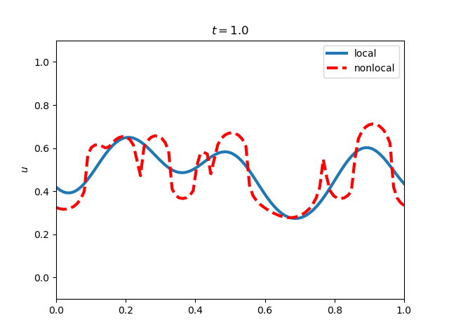
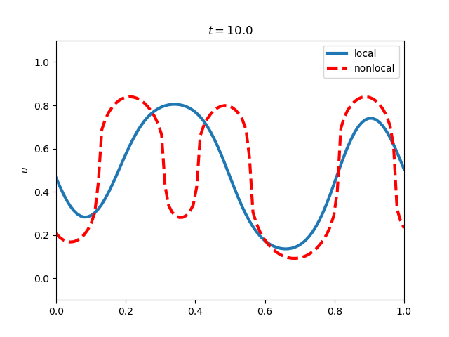
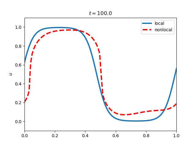
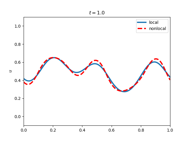
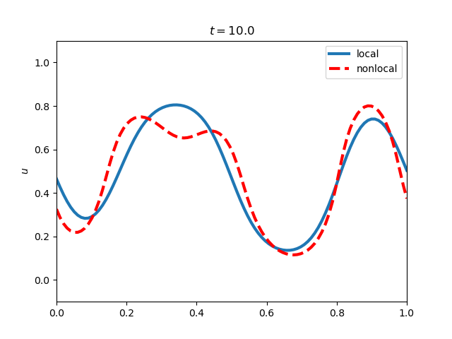
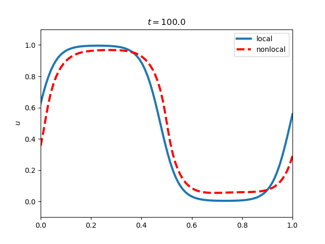
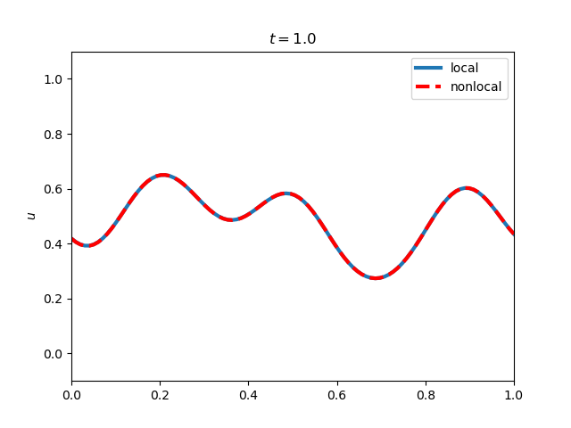
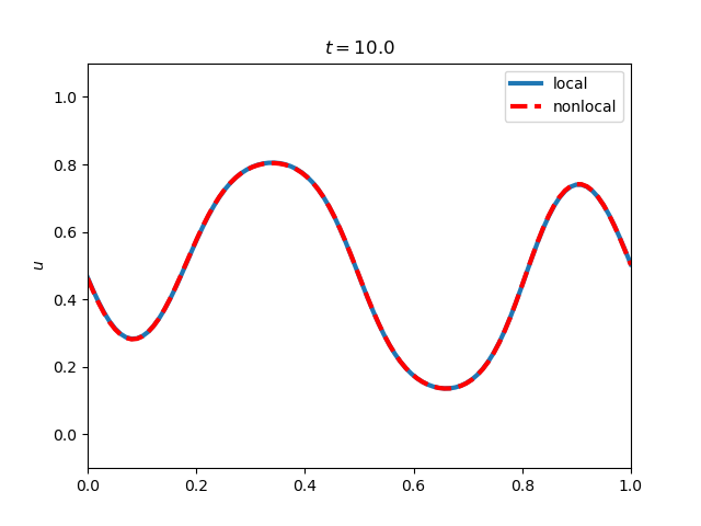
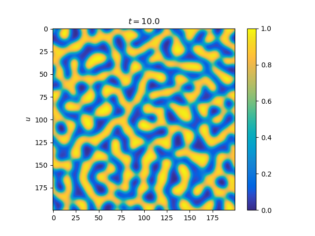
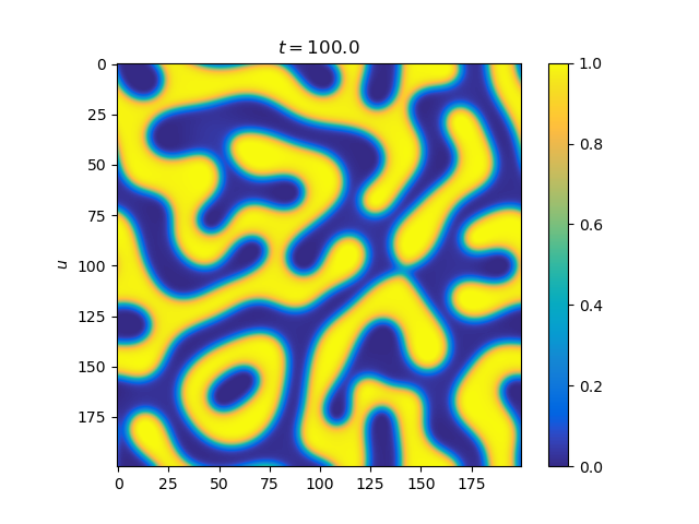
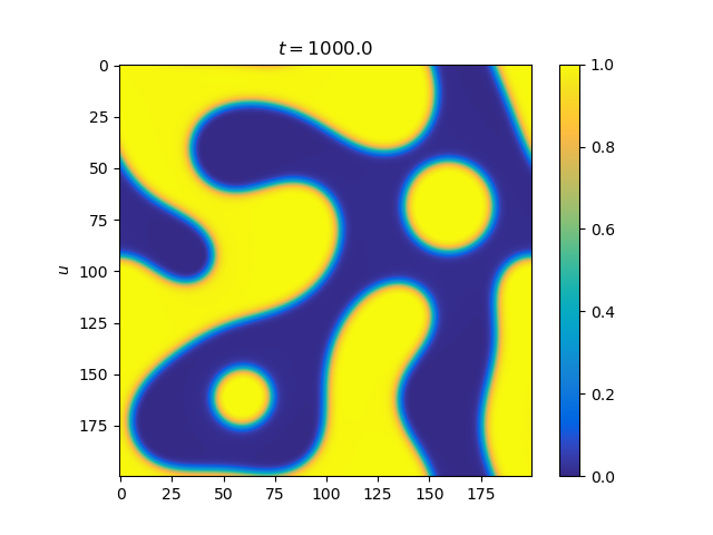
5 Numerical simulations
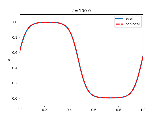
To illustrate the behavior of the solutions as , we propose numerical simulations. To keep things simple, we assume that the mobility is constant, , and we use a smooth approximation of the double-well potential in Equations (1.9)-(1.10) and (1.11)-(1.12). We refer to [6], where authors investigate how the non-smooth nature of the double-well potential (such as the double-obstacle potential) generates sharp interfaces.
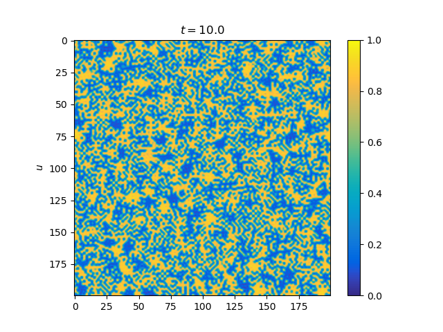
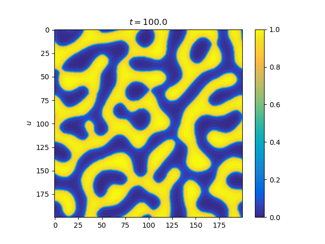
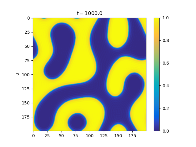
Our simulations are made in both one and two dimensions. The kernel reads
We consider three specific scenarios: , , and . In the one-dimensional case, we superimpose the curve of the nonlocal solution (represented in red) onto the curve of the local solution (depicted in blue). We observe their evolution over time at , , and .
In the two-dimensional case, the first row showcases the evolution of the nonlocal Cahn-Hilliard equation at , , and . The last row represents the evolution of the local equation.
The numerical implementation was made using Python, and numpy.fft, numpy.ifft to efficiently compute the Fourier and inverse Fourier transforms. The Fourier transform is particularly useful for terms like
and the convolution .
Focusing on the numerical results, the observations made in both one and two dimensions are the same. As is sent to zero, the solutions of the non-local equation converge to those of the local equation. When is set to 0.1, the difference becomes invisible to the naked eye.
We opted for a random initial condition with low regularity. Within the simulations for both one-dimensional and two-dimensional scenarios with , we observe two interesting aspects. First, the regularity of solutions to the nonlocal equation is lower than that of the local one and the initial condition requires a longer time to be smoothed. From a theoretical point of view, this can be explained by the regularity (a porous medium character) for the nonlocal equation compared to the regularity for the local equation. The second point of interest lies in the formation of an interface in a long time which is of different nature for both equations. For, , at the final time step, the interface is sharp, unlike the diffuse interface observed for the local equation.
6 The nonlocal-to-local limit for the cell-cell adhesion model
Here, we explain, using similar ideas, how to treat a recently introduced model in the theory of cell-cell adhesion from [13, eq. (15)] which also involves the mobility . More precisely, we consider the PDE posed on
| (6.1) |
where the parameter measures the relative cell-cell adhesion strength while is the nonlocal kernel defined as
Here, is a smooth, radially symmetric and compactly supported kernel with and is a unit sphere in . It is useful to observe that, with the assumptions on , can be written as a convolution operator
We now rescale the kernel by taking in (6.1) where and is a smooth, radially symmetric and compactly supported kernel. The scaling factor is chosen to obtain a meaningful PDE in the limit as explained below. Hence, we consider solutions to the PDE
| (6.2) |
with
| (6.3) |
and we want to understand the limit . To guess what is the expected PDE, let . Then, by Taylor’s expansion,
| (6.4) |
where when . Hence, we expect that the limiting PDE reads
| (6.5) |
where .
To have sufficient uniform a priori estimates with respect to , we have to assume that the parameter satisfies
| (6.6) |
where is a constant in the inequality
| (6.7) |
which holds true by Lemma C.2. The inequality (6.7) implies also the uniform bound on : using that we have
so that by Jensen’s inequality
| (6.8) |
For the nonlocal-to-local limit, the main idea is again the same as in the case of the Cahn-Hilliard system: the mobility ensures that the solution remains bounded so that we can easily handle the nonlinear terms. We also want to comment that in [13] Authors derive also systems of PDEs of the form (6.2) but these are not treatable mathematically because, in full generality, there is currently no mathematical theory of such systems. Here we focus on a single equation.
6.1 Existence of weak solutions to (6.2)
Definition 6.1.
We say that a function is a weak solution to (6.2) with initial condition if and for all we have
Lemma 6.2.
Proof.
Step 1: An auxiliary problem. For fixed we consider an auxiliary problem
| (6.9) |
where is a standard mollifying sequence. A solution to (6.9) with regularity can be obtained by standard methods, for example by the Schauder’s fixed point theorem. We want to pass with in (6.9).
Step 2: Uniform bounds with respect to and . We claim that the following sequences are uniformly bounded with respect to :
-
(F1)
in with ,
-
(F2)
in ,
-
(F3)
in .
Let be a function such that for and for . Let . Integrating in space we deduce
Since and , we can approximate function with and deduce
where . The integrand on the (RHS) can be written again in the divergence form as so the respective integral vanish and we conclude that . In a similar way we prove that .
Next, we multiply by and integrate by parts to get
| (6.10) |
Using (6.8), we obtain
Hence, since , we obtain (F2).
Step 3: The limit and the estimates (E1)–(E3). By the Aubin-Lions lemma, the Banach-Alaoglu theorem and interpolation in spaces, there exists a subsequence such that
| (6.11) |
This is sufficient to pass to the limit in the expression
(keep in mind that is fixed!) for so that satisfies Definition 6.1. Finally, since bounds (F1)–(F3) are preserved along the limit (6.11), (E1)–(E3) follow.
∎
6.2 Passing to the limit in (6.2).
Theorem 6.3.
Proof.
As in the proof of Lemma 6.2, by the Aubin-Lions lemma, the Banach-Alaoglu theorem, interpolation in spaces and the bounds (E1)–(E3), there exists a subsequence as in (6.12).
We want to pass to the limit in Definition 6.1. The only difficulty is to justify the limit in the term
| (6.13) |
due to the singularity in the nonlocal operator . By the bound (6.8), there exists such that
To identify , let . Since is a convolution operator with an antisymmetric kernel (see 6.3)
| (6.14) |
By (6.4), so that passing to the limit in (6.14) we obtain
which implies . Furthermore, by (6.12),
so that we can pass to the limit in (6.13)
and the proof is concluded. ∎
Acknowledgements
Jakub Skrzeczkowski was supported by the Advanced Grant Nonlocal-CPD (Nonlocal PDEs for Complex Particle Dynamics: Phase Transitions, Patterns and Synchronization) of the European Research Council Executive Agency (ERC) under the European Union’s Horizon 2020 research and Innovation programme (grant agreement No. 883363).
Appendix A Results from classical analysis
Lemma A.1.
Let be a sequence strongly compact in . Then,
Proof.
We write
Therefore
With the assumptions of the lemma, we deduce that the first term converges to 0 uniformly with respect to . Concerning the second term, we use the Fréchet-Kolmogorov theorem to deduce that the translation converge to 0 uniformly: there exists a modulus of continuity such that and
This proves the result. ∎
Appendix B Bourgain-Brézis-Mironescu and Ponce compactness result
We consider a sequence of radial functions such that , and
For the formulation of the compactness result, we use another sequence of standard mollifiers with mass 1 such that with of mass 1 and compactly supported.
Theorem B.1.
Let . Let be a sequence bounded in . Suppose that there exists a sequence as above such that
| (B.1) |
for some constant . Then, is compact in space in , i.e.
| (B.2) |
Appendix C Nonlocal Poincaré inequalities
Let be a smooth function, supported in the unit ball such that . Consider .
Lemma C.1.
For all , there exists and such that
for every and .
For the proof, we refer to Ponce [55, Theorem 1.1]. We also have an opposite inequality from [3, Theorem 1]:
Lemma C.2.
For all , there exists a constant such that for all
Finally, we formulate a variant of Lemma C.1 which does not require an average on the left-hand side. The proof can be adapted from [25, Lemma C.3].
Lemma C.3.
For each there exists and constant such that for all and all we have
References
- [1] H. Abels and C. Hurm. Strong nonlocal-to-local convergence of the Cahn-Hilliard equation and its operator. J. Differential Equations, 402:593–624, 2024.
- [2] G. Alberti and G. Bellettini. A nonlocal anisotropic model for phase transitions. I. The optimal profile problem. Math. Ann., 310(3):527–560, 1998.
- [3] J. Bourgain, H. Brezis, and P. Mironescu. Another look at Sobolev spaces. In Optimal control and partial differential equations, pages 439–455. IOS, Amsterdam, 2001.
- [4] M. Burger, M. Di Francesco, J.-F. Pietschmann, and B. Schlake. Nonlinear cross-diffusion with size exclusion. SIAM J. Math. Anal., 42(6):2842–2871, 2010.
- [5] M. Burger and A. Esposito. Porous medium equation and cross-diffusion systems as limit of nonlocal interaction. Nonlinear Anal., 235:Paper No. 113347, 30, 2023.
- [6] O. Burkovska and M. Gunzburger. On a nonlocal Cahn-Hilliard model permitting sharp interfaces. Math. Models Methods Appl. Sci., 31(9):1749–1786, 2021.
- [7] J. W. Cahn. On spinodal decomposition. Acta Metallurgica, 9(9):795–801, 1961.
- [8] J. W. Cahn and J. E. Hilliard. Free energy of a nonuniform system. I. Interfacial Free Energy. The Journal of Chemical Physics, 28(2):258–267, 1958.
- [9] J. A. Carrillo, K. Craig, and F. S. Patacchini. A blob method for diffusion. Calc. Var. Partial Differential Equations, 58(2):Paper No. 53, 53, 2019.
- [10] J. A. Carrillo, C. Elbar, and J. Skrzeczkowski. Degenerate cahn-hilliard systems: From nonlocal to local. arXiv preprint arXiv:2303.11929, to appear in Commun. Contemp. Math., 2023.
- [11] J. A. Carrillo, A. Esposito, and J. S.-H. Wu. Nonlocal approximation of nonlinear diffusion equations. Calc. Var. Partial Differential Equations, 63(4):Paper No. 100, 44, 2024.
- [12] J. A. Carrillo, S. Lisini, G. Savaré, and D. Slepčev. Nonlinear mobility continuity equations and generalized displacement convexity. J. Funct. Anal., 258(4):1273–1309, 2010.
- [13] J. A. Carrillo, H. Murakawa, M. Sato, H. Togashi, and O. Trush. A population dynamics model of cell-cell adhesion incorporating population pressure and density saturation. J. Theoret. Biol., 474:14–24, 2019.
- [14] J. A. Carrillo, L. Wang, and C. Wei. Structure preserving primal dual methods for gradient flows with nonlinear mobility transport distances. SIAM J. Numer. Anal., 62(1):376–399, 2024.
- [15] L. Cherfils, H. Fakih, M. Grasselli, and A. Miranville. A convergent convex splitting scheme for a nonlocal Cahn-Hilliard-Oono type equation with a transport term. ESAIM Math. Model. Numer. Anal., 55(suppl.):S225–S250, 2021.
- [16] G. M. Coclite, M. Colombo, G. Crippa, N. De Nitti, A. Keimer, E. Marconi, L. Pflug, and L. V. Spinolo. Oleinik-type estimates for nonlocal conservation laws and applications to the nonlocal-to-local limit. arXiv preprint arXiv:2304.01309, 2023.
- [17] N. David, T. Dębiec, M. Mandal, and M. Schmidtchen. A degenerate cross-diffusion system as the inviscid limit of a nonlocal tissue growth model. SIAM J. Math. Anal., 56(2):2090–2114, 2024.
- [18] E. Davoli, H. Ranetbauer, L. Scarpa, and L. Trussardi. Degenerate nonlocal Cahn-Hilliard equations: well-posedness, regularity and local asymptotics. Ann. Inst. H. Poincaré C Anal. Non Linéaire, 37(3):627–651, 2020.
- [19] E. Davoli, L. Scarpa, and L. Trussardi. Local asymptotics for nonlocal convective Cahn-Hilliard equations with kernel and singular potential. J. Differential Equations, 289:35–58, 2021.
- [20] E. Davoli, L. Scarpa, and L. Trussardi. Nonlocal-to-local convergence of Cahn-Hilliard equations: Neumann boundary conditions and viscosity terms. Arch. Ration. Mech. Anal., 239(1):117–149, 2021.
- [21] J. Dolbeault, B. Nazaret, and G. Savaré. A new class of transport distances between measures. Calc. Var. Partial Differential Equations, 34(2):193–231, 2009.
- [22] M. Doumic, S. Hecht, B. Perthame, and D. Peurichard. Multispecies cross-diffusions: from a nonlocal mean-field to a porous medium system without self-diffusion. J. Differential Equations, 389:228–256, 2024.
- [23] C. Elbar, B. Perthame, A. Poiatti, and J. Skrzeczkowski. Nonlocal Cahn–Hilliard Equation with Degenerate Mobility: Incompressible Limit and Convergence to Stationary States. Arch. Ration. Mech. Anal., 248(3):Paper No. 41, 2024.
- [24] C. Elbar, B. Perthame, and J. Skrzeczkowski. Pressure jump and radial stationary solutions of the degenerate Cahn–Hilliard equation. Comptes Rendus. Mécanique, 351(S1):375–394, 2023.
- [25] C. Elbar and J. Skrzeczkowski. Degenerate Cahn-Hilliard equation: From nonlocal to local. J. Differential Equations, 364:576–611, 2023.
- [26] C. Elbar and J. Skrzeczkowski. On the inviscid limit connecting Brinkman’s and Darcy’s models of tissue growth with nonlinear pressure. arXiv preprint arXiv:2306.03752, 2023.
- [27] C. M. Elliott and H. Garcke. On the Cahn-Hilliard equation with degenerate mobility. SIAM J. Math. Anal., 27(2):404–423, 1996.
- [28] C. Falcó, R. E. Baker, and J. A. Carrillo. A local continuum model of cell-cell adhesion. arXiv preprint arXiv:2206.14461; to appear in SIAM J. Appl. Math., 2022.
- [29] S. Frigeri. On a nonlocal Cahn-Hilliard/Navier-Stokes system with degenerate mobility and singular potential for incompressible fluids with different densities. Ann. Inst. H. Poincaré C Anal. Non Linéaire, 38(3):647–687, 2021.
- [30] S. Frigeri, C. G. Gal, and M. Grasselli. On nonlocal Cahn-Hilliard-Navier-Stokes systems in two dimensions. J. Nonlinear Sci., 26(4):847–893, 2016.
- [31] S. Frigeri, C. G. Gal, and M. Grasselli. Regularity results for the nonlocal Cahn-Hilliard equation with singular potential and degenerate mobility. J. Differential Equations, 287:295–328, 2021.
- [32] S. Frigeri, C. G. Gal, M. Grasselli, and J. Sprekels. Two-dimensional nonlocal Cahn-Hilliard-Navier-Stokes systems with variable viscosity, degenerate mobility and singular potential. Nonlinearity, 32(2):678–727, 2019.
- [33] S. Frigeri and M. Grasselli. Nonlocal Cahn-Hilliard-Navier-Stokes systems with singular potentials. Dyn. Partial Differ. Equ., 9(4):273–304, 2012.
- [34] S. Frigeri, M. Grasselli, and P. Krejčí. Strong solutions for two-dimensional nonlocal Cahn-Hilliard-Navier-Stokes systems. J. Differential Equations, 255(9):2587–2614, 2013.
- [35] S. Frigeri, M. Grasselli, and E. Rocca. A diffuse interface model for two-phase incompressible flows with non-local interactions and non-constant mobility. Nonlinearity, 28(5):1257–1293, 2015.
- [36] H. Gajewski and K. Zacharias. On a nonlocal phase separation model. J. Math. Anal. Appl., 286(1):11–31, 2003.
- [37] C. G. Gal, A. Giorgini, and M. Grasselli. The nonlocal Cahn-Hilliard equation with singular potential: well-posedness, regularity and strict separation property. J. Differential Equations, 263(9):5253–5297, 2017.
- [38] C. G. Gal, A. Giorgini, and M. Grasselli. The separation property for 2D Cahn-Hilliard equations: local, nonlocal and fractional energy cases. Discrete Contin. Dyn. Syst., 43(6):2270–2304, 2023.
- [39] C. G. Gal and M. Grasselli. Longtime behavior of nonlocal Cahn-Hilliard equations. Discrete Contin. Dyn. Syst., 34(1):145–179, 2014.
- [40] G. Giacomin and J. L. Lebowitz. Phase segregation dynamics in particle systems with long range interactions. I. Macroscopic limits. J. Statist. Phys., 87(1-2):37–61, 1997.
- [41] G. Giacomin and J. L. Lebowitz. Phase segregation dynamics in particle systems with long range interactions. II. Interface motion. SIAM J. Appl. Math., 58(6):1707–1729, 1998.
- [42] P. Knopf and A. Signori. On the nonlocal Cahn–Hilliard equation with nonlocal dynamic boundary condition and boundary penalization. J. Differential Equations, 280(4):236–291, 2021.
- [43] P.-L. Lions and S. Mas-Gallic. Une méthode particulaire déterministe pour des équations diffusives non linéaires. C. R. Acad. Sci. Paris Sér. I Math., 332(4):369–376, 2001.
- [44] S. Lisini and A. Marigonda. On a class of modified Wasserstein distances induced by concave mobility functions defined on bounded intervals. Manuscripta Math., 133(1-2):197–224, 2010.
- [45] S. Lisini, D. Matthes, and G. Savaré. Cahn-Hilliard and thin film equations with nonlinear mobility as gradient flows in weighted-Wasserstein metrics. J. Differential Equations, 253(2):814–850, 2012.
- [46] D. Loibl, D. Matthes, and J. Zinsl. Existence of weak solutions to a class of fourth order partial differential equations with Wasserstein gradient structure. Potential Anal., 45(4):755–776, 2016.
- [47] S.-O. Londen and H. Petzeltová. Convergence of solutions of a non-local phase-field system. Discrete Contin. Dyn. Syst. Ser. S, 4(3):653–670, 2011.
- [48] S.-O. Londen and H. Petzeltová. Regularity and separation from potential barriers for a non-local phase-field system. J. Math. Anal. Appl., 379(2):724–735, 2011.
- [49] D. Matthes and J. Zinsl. Existence of solutions for a class of fourth order cross-diffusion systems of gradient flow type. Nonlinear Anal., 159:316–338, 2017.
- [50] S. Melchionna, H. Ranetbauer, L. Scarpa, and L. Trussardi. From nonlocal to local Cahn-Hilliard equation. Adv. Math. Sci. Appl., 28(2):197–211, 2019.
- [51] S. Melchionna and E. Rocca. On a nonlocal Cahn-Hilliard equation with a reaction term. Adv. Math. Sci. Appl., 24(2):461–497, 2014.
- [52] A. Miranville. The Cahn-Hilliard equation. Recent advances and applications, volume 95 of CBMS-NSF Regional Conference Series in Applied Mathematics. Society for Industrial and Applied Mathematics (SIAM), Philadelphia, PA, 2019. Recent advances and applications.
- [53] B. Perthame and A. Poulain. Relaxation of the Cahn-Hilliard equation with singular single-well potential and degenerate mobility. European J. Appl. Math., 32(1):89–112, 2021.
- [54] A. Poiatti. The 3D strict separation property for the nonlocal Cahn-Hilliard equation with singular potential. arXiv preprint arXiv:2303.07745; to appear in Analysis & PDEs, 2023.
- [55] A. C. Ponce. An estimate in the spirit of Poincaré’s inequality. J. Eur. Math. Soc. (JEMS), 6(1):1–15, 2004.
- [56] E. Rocca, L. Scarpa, and A. Signori. Parameter identification for nonlocal phase field models for tumor growth via optimal control and asymptotic analysis. Math. Models Methods Appl. Sci., 31(13):2643–2694, 2021.
- [57] H. Wu. A review on the Cahn-Hilliard equation: classical results and recent advances in dynamic boundary conditions. Electron. Res. Arch., 30(8):2788–2832, 2022.