On the convergence of generalized kernel-based interpolation by greedy data selection algorithms

Abstract

Besides standard Lagrange interpolation, i.e., interpolation of target functions from scattered point evaluations, positive definite kernel functions are well-suited for the solution of more general reconstruction problems. This is due to the intrinsic structure of the underlying reproducing kernel Hilbert space (RKHS). In fact, kernel-based interpolation has been applied to the reconstruction of bivariate functions from scattered Radon samples in computerized tomography (cf. [10]) and, moreover, to the numerical solution of elliptic PDEs (cf. [20]). As shown in various previous contributions, numerical algorithms and theoretical results from kernel-based Lagrange interpolation can be transferred to more general interpolation problems. In particular, greedy point selection methods were studied in [20], for the special case of Sobolev kernels. In this paper, we aim to develop and analyze more general kernel-based interpolation methods, for less restrictive settings. To this end, we first provide convergence results for generalized interpolation under minimalistic assumptions on both the selected kernel and the target function. Finally, we prove convergence of popular greedy data selection algorithms for totally bounded sets of functionals. Supporting numerical results are provided for illustration.

1 Introduction

Kernel functions provide powerful numerical methods for multivariate scattered data approximation [18]. Positive definite or conditionally positive definite radial kernels — previously also referred to as radial basis functions (RBF) [3] — were primarily used to interpolate multivariate scalar-valued functions from Lagrange data. In that particular case, finitely many scalar samples are taken from a (multivariate) target function by the application of Dirac point evaluation functionals on shifted scattered points. A more comprehensive discussion on multivariate Lagrange interpolation by (conditionally) positive definite functions can be found in [3, 18].

Possible extensions of kernel-based Lagrange interpolation are working with more general evaluation functionals, rather than just Dirac point evaluations. One classical example are evaluations of (directional) derivatives, whose samples are called Hermite data. Other extensions include Radon data (i.e., from line integrals, cf. [4]) or cell averages (e.g., in finite volume methods, cf. [2]).

As shown in [9, 21], the concept of kernel-based interpolation from samples taken by (linear) functionals can be unified to obtain the more general Hermite-Birkhoff interpolation scheme, which is throughout this paper called generalized kernel-based interpolation, cf. [18, Chapter 16].

As regards the theory of kernel-based interpolation, we remark that positive definite kernels generate a reproducing kernel Hilbert space (RKHS), i.e., the kernel’s native space (cf. [18, Chapter 10]). For the error analysis of kernel-based interpolation, the pointwise error functional (lying in the dual space of the RKHS) plays a central role. In fact, available results on the convergence and approximation orders of kernel-based interpolation involve the norm of the pointwise error functional, called power function (cf. [18, Chapter 10]).

One important ingredient for the development of stable kernel-based interpolation algorithms are Newton bases (cf. [13, 14]). Moreover, the implementation of greedy algorithms (cf. [19]) for the selection of suitable sample points, plays an important role for the performance of kernel-based interpolation schemes, especially for their stability and efficiency. We remark that the above mentioned ingredients (i.e., power function, Newton bases, greedy algorithms) can be transferred to generalized kernel-based interpolation in the kernel’s RKHS.

To make only one example, greedy algorithms were recently used in [20] to solve elliptic PDEs by meshfree kernel methods. In the particular problem of [20], the utilized kernel is required to be sufficiently smooth, which then led to convergence rates in the kernel’s native Sobolev space.

It is important to note that there are relevant applications where it is not desirable at all to work with smooth kernels. One relevant example are WENO schemes for the numerical solution of hyperbolic conservation laws [11], another one is concerning applications of computerized tomography [4], where less restrictive assumptions on the regularity of the target are essentially required.

This gives rise to work with rougher kernels, leading to larger native spaces containing rougher (target) functions. In this paper, we prove convergence results for generalized kernel-based interpolation schemes under mild restrictions on the kernel function’s regularity, i.e., for rougher kernels.

The outline of this paper is as follows. In Section 2, we introduce key ingredients of generalized kernel-based interpolation, including the native space and the power function. In Section 3, we first prove a convergence criterion (Theorem 3.1), involving the asymptotic behaviour of the power function, on which we then prove convergence of generalized kernel-based interpolation (Theorem 3.2) under rather mild assumptions. In Section 4, we use Theorem 3.2 to prove convergence for two popular classes of greedy algorithms: the $\beta$-greedy algorithm (Theorem 4.4) and the geometric greedy algorithm of [5] (Theorem 4.5). Supporting numerical results on kernel-based interpolation from scattered Radon data are presented in Section 5.

2 Generalized kernel-based interpolation

We consider a positive definite function $K:\mathbb{R}^{d}\times\mathbb{R}^{d}\longrightarrow\mathbb{R}$, i.e., $K$ is symmetric and for any finite set $X=\{x_{1},\ldots,x_{n}\}\subset\mathbb{R}^{d}$ of pairwise distinct points, the matrix

$$A_{K,X}:=\left(K(x_{i},x_{j})\right)_{1\leq i,j\leq n}\in\mathbb{R}^{n\times n}$$

is symmetric positive definite (see [10, 18]). Recall that that any positive definite function $K$ generates a reproducing kernel Hilbert space (RKHS) $\mathcal{H}_{K}$, so that the reproduction

$$f(x)=\langle f,K(\cdot,x)\rangle_{\mathcal{H}_{K}}\qquad\text{ for all }f\in\mathcal{H}_{K}\text{ and all }x\in\mathbb{R}^{d}$$ (1)

holds. Therefore, $K$ is referred to as a kernel function. Moreover, $\mathcal{H}_{K}$ is called the kernel’s native space. An essential part of generalized interpolation in $\mathcal{H}_{K}$ is that the reproduction in (1) can be transferred to the dual space $\mathcal{H}_{K}^{*}$ of $\mathcal{H}_{K}$.

Proposition 2.1 ([18, Theorem 16.7]).

Let $\lambda\in\mathcal{H}_{K}^{*}$. For the function

$$\lambda^{y}K(\cdot,y):\mathbb{R}^{d}\longrightarrow\mathbb{R},\qquad x\longmapsto\lambda^{y}K(x,y),$$

we have $\lambda^{y}K(\cdot,y)\in\mathcal{H}_{K}$. Moreover, the generalized reproduction holds, i.e.,

$$\lambda(f)=\langle f,\lambda^{y}K(\cdot,y)\rangle_{\mathcal{H}_{K}}\qquad\text{ for all }f\in\mathcal{H}_{K}.$$ (2)

Note that Proposition 2.1 allows us to compute the Riesz representers for functionals from the dual space $\mathcal{H}_{K}^{*}$ explicitely, which gives an advantage over the general Hilbert space setting.

Now suppose that $\Lambda=\{\lambda_{1},...,\lambda_{n}\}\subset\mathcal{H}_{K}^{*}$ is a finite set of pairwise distinct linear functionals. Given a function $f\in\mathcal{H}_{K}$ and scalar samples $\lambda_{1}(f),\ldots,\lambda_{n}(f)$ of $f$ on $\Lambda$, the generalized interpolation problem requires finding a function $s\equiv s_{f,\Lambda}$ from the finite dimensional linear subspace

$$S_{K,\Lambda}:=\text{span}\;\{\lambda_{1}^{y}K(\cdot,y),...,\lambda_{n}^{y}K(\cdot,y)\}\subset\mathcal{H}_{K},$$

such that the interpolation conditions

$$\lambda_{i}(f)=\lambda_{i}(s)\qquad\text{ for all }i=1,\ldots,n$$ (3)

are satisfied. If the linear functionals in $\Lambda$ are linearly independent, then there is a unique solution $s$ to the interpolation problem (3), cf. [18, Theorem 16.1]). Thereby, we can define an interpolation operator

$$I_{K,\Lambda}:\mathcal{H}_{K}\longrightarrow S_{K,\Lambda},\qquad f\longmapsto s_{f,\Lambda}.$$

Due to the generalized reproduction in (2), the interpolant $s\equiv s_{f,\Lambda}$ coincides with the orthogonal projection of $f$ onto $S_{K,\Lambda}$, in which case there is an efficient and stable computation of $s$ by using orthonormal bases.

In our convergence analysis for generalized kernel-based interpolation, we consider, for a fixed subset of functionals $\Gamma\subset\mathcal{H}_{K}^{*}$, nested sequences $\left(\Lambda_{n}\right)_{n\in\mathbb{N}}$ of finite subsets $\Lambda_{n}\subset\Gamma$, each containing linearly independent functionals.

Our general aim is to develop mild conditions on sequences $\left(\Lambda_{n}\right)_{n\in\mathbb{N}}$ under which the convergence

$$\|f-I_{K,\Lambda_{n}}(f)\|_{K}\xrightarrow{n\to\infty}0$$ (4)

holds for all target functions $f\in\mathcal{H}_{K,\Gamma}$ from the closed linear subspace

$$\mathcal{H}_{K,\Gamma}=\overline{\text{span}\;\{\lambda^{y}K(\cdot,y)\mid\lambda\in\Gamma\}}\subset\mathcal{H}_{K}.$$

We recall that the sequence $(I_{K,\Lambda_{n}}(f))_{n\in\mathbb{N}}$ of interpolants convergences in $\mathcal{H}_{K,\Gamma}$. For further details on this, we refer to the second statement in Lemma 4.3.

In the theory of standard kernel-based Lagrange interpolation, the pointwise error functional is an element in the dual $\mathcal{H}_{K}^{*}$ of the native space $\mathcal{H}_{K}$, whose (native space) norm, called power function, leads to an upper bound for pointwise error estimates.

It is rather straightforward to extend the power function of kernel-based Lagrange interpolation to the more general setting of this section: For a given linearly independent set $\Lambda\subset\mathcal{H}_{K}^{*}$, the generalized power function is defined as

$$P_{\Lambda}(\lambda):=\|\lambda^{y}K(\cdot,y)-I_{K,\Lambda}(\lambda^{y}K(\cdot,y))\|_{\mathcal{H}_{K}}\qquad\text{ for }\lambda\in\Gamma.$$

Note that the power function $P_{\Lambda}$ measures the $\|\cdot\|_{\mathcal{H}_{K}}$-norm distance between the Riesz representer $\lambda^{y}K(\cdot,y)$ and the linear space $S_{K,\Lambda}$, by the orthogonal projection property of the interpolation operator $I_{K,\Lambda}$. As a direct consequence of the representation theorem, Proposition 2.1, we have for $\lambda\in\Gamma$ the equivalence

$$P_{\Lambda}(\lambda)=0\quad\Longleftrightarrow\quad\lambda^{y}K(\cdot,y)\in S_{K,\Lambda}\quad\Longleftrightarrow\quad\lambda\in\text{span}\;(\Lambda).$$

Hence, the power function can be interpreted as a measurement of the linear dependence between functionals in $\Gamma$. It can also be shown that the power function $P_{\Lambda}$ yields the upper bound

$$|\lambda(f)-\lambda(I_{K,\Lambda}(f))|\leq P_{\Lambda}(\lambda)\cdot\|f\|_{\mathcal{H}_{K}}\qquad\text{ for }f\in\mathcal{H}_{K}$$

for the pointwise interpolation error. Another error indicator is the fill distance

$$h_{\Lambda,\Gamma}:=\underset{\lambda\in\Gamma}{\sup}\;\underset{i=1,...,n}{\min}\;\|\lambda-\lambda_{i}\|_{\mathcal{H}_{K}^{*}}.$$

The fill distance can be viewed as the radius of the largest open ball with midpoint in $\Gamma$ that does not contain any point from $\Lambda$. We will make more sense of this geometric description in the next section.

Remark 2.2.

So far, it may not be clear how we can compute the power function and the interpolants in numercial tests. As was already pointed out in [20], the Newton basis from [13] and its respective update formula from [14] can be adapted to the case of generalized interpolation. Hence, (update) formulas for the power function and the interpolants are also available.

3 Convergence under mild conditions

If we take a closer look at the desired convergence (4), we see that this already includes the condition

$$P_{\Lambda_{n}}(\lambda)=\|\lambda^{y}K(\cdot,y)-I_{K,\Lambda}(\lambda^{y}K(\cdot,y))\|_{\mathcal{H}_{K}}\xrightarrow{n\to\infty}0\qquad\text{for all }\lambda\in\Gamma,$$

by definition of the subspace $\mathcal{H}_{K,\Gamma}\subset\mathcal{H}_{K}$. Therefore, the pointwise decay of the power functions is a necessary condition. We can show that it is even sufficient for the normwise convergence of the interpolation method on the whole space.

Theorem 3.1.

Let $\Gamma\subset\mathcal{H}_{K}^{*}$ and $\left(\Lambda_{n}\right)_{n\in\mathbb{N}}$ be a nested sequence of finite linearly independent subsets of $\Gamma$. Then, the generalized interpolation method converges on $\mathcal{H}_{K,\Gamma}$, i.e.,

$$\|f-I_{K,\Lambda_{n}}(f)\|_{\mathcal{H}_{K}}\xrightarrow{n\to\infty}0\qquad\text{for all }f\in\mathcal{H}_{K,\Gamma},$$

if and only if the power functions converges pointwise to zero on $\Gamma$, i.e.

$$P_{\Lambda_{n}}(\lambda)\xrightarrow{n\to\infty}0\qquad\text{for all }\lambda\in\Gamma.$$

Proof.

First, we consider an element

$$s=\sum\limits_{i=1}^{N}c_{i}\mu_{i}^{y}K(\cdot,y)\in\text{span}_{\mathbb{R}}\;\{\lambda^{y}K(\cdot,y)\mid\lambda\in\Gamma\}=:S_{K,\Gamma}.$$

Since $I_{K,\Lambda_{n}}$ is a linear operator for each $n\in\mathbb{N}$, we get the convergence

$$\|s-I_{K,\Lambda_{n}}(s)\|_{\mathcal{H}_{K}} =\Big{\|}\sum\limits_{i=1}^{N}c_{i}\cdot\left(\mu_{i}^{y}K(\cdot,y)-I_{K,\Lambda_{n}}(\mu_{i}^{y}K(\cdot,y))\right)\Big{\|}_{\mathcal{H}_{K}}$$

$$\leq\sum\limits_{i=1}^{N}|c_{i}|\cdot P_{\Lambda_{n}}(\mu_{i})\xrightarrow{n\to\infty}0.$$

Due to the density of $S_{K,\Gamma}$ in $\mathcal{H}_{K,\Gamma}$, the stated convergence on $\mathcal{H}_{K,\Gamma}$ holds. ∎

Similarly, we can derive a convergence condition with respect to the fill distances $h_{\Lambda_{n},\Gamma}$. It should be mentioned here that this only represents a sufficient condition, and the decay of the fill distances might not be necessary for the convergence of the interpolation method.

Theorem 3.2.

Let $\Gamma\subset\mathcal{H}_{K}^{*}$ and $\left(\Lambda_{n}\right)_{n\in\mathbb{N}}$ be a nested sequence of finite linearly independent subsets of $\Gamma$ that satisfies $h_{\Lambda_{n},\Gamma}\searrow 0$ for $n\to\infty$. Then we have

$$\|f-I_{K,\Lambda_{n}}(f)\|_{\mathcal{H}_{K}}\xrightarrow{n\to\infty}0\qquad\text{for all }f\in\mathcal{H}_{K,\Gamma}.$$

Proof.

It is easy to see that the fill distance is a uniform bound for the power function, so that we immediately get

$$P_{\Lambda_{n}}(\lambda)\leq h_{\Lambda_{n},\Gamma}\xrightarrow{n\to\infty}0\qquad\text{for all }\lambda\in\Gamma.$$

Therefore, Theorem 3.1 yields the stated convergence. ∎

A key feature of native RKHS is that the norm convergence automatically implies pointwise convergence to the target function $f$. If the chosen kernel $K$ is bounded, we even have uniform convergence for the interpolation method.

Corollary 3.3.

In the setting of Theorem 3.1 or Theorem 3.2, we also have uniform convergence

$$\|f-I_{K,\Lambda_{n}}(f)\|_{\infty}=\underset{x\in\mathbb{R}^{d}}{\sup}\;|f(x)-I_{K,\Lambda_{n}}[f](x)|\xrightarrow{n\to\infty}0,$$

if $K$ is bounded.

Proof.

This follows from our previous results and the standard estimate

$$|f(x)-I_{K,\Lambda_{n}}[f](x)| =|\langle f-I_{K,\Lambda_{n}}(f),K(\cdot,x)\rangle_{\mathcal{H}_{K}}|$$

$$\leq\underset{x\in\mathbb{R}^{d}}{\sup}\;\sqrt{K(x,x)}\cdot\|f-I_{K,\Lambda_{n}}(f)\|_{\mathcal{H}_{K}},$$

as we have $\|K(\cdot,x)\|_{\mathcal{H}_{K}}=\sqrt{K(x,x)}$ for all $x\in\mathbb{R}^{d}$. ∎

3.1 Parameterization

In many cases, the superset $\Gamma\subset\mathcal{H}_{K}^{*}$ is parameterized by a much simpler space. For example, the point evaluation functionals are parameterized by the mapping

$$\varrho:\mathbb{R}^{d}\longrightarrow\mathcal{H}_{K}^{*},\qquad x\longmapsto\delta_{x}.$$

One main advantage of parameterizations is that, in general, many computations like evaluations of norms are less costly than in the native dual space. Instead of finding suitable sets of data points in the dual space, we can search for good data points in the parameter space. If the parameterization map $\varrho$ is uniformly continuous, the decay of the fill distance in the parameter space then translates to the decay of the fill distance in the dual space.

Theorem 3.4.

Let $\Gamma\subset\mathcal{H}_{K}^{*}$ be linearly independent. Moreover, let $\left(\Omega,d_{\Omega}\right)$ be a metric space and $\varrho:\Omega\longrightarrow\Gamma$ be uniformly continuous and bijective. If $\left(X_{n}\right)_{n\in\mathbb{N}}$ is a nested sequence of finite subsets from $\Omega$ satisfying $h_{X_{n},\Omega}\searrow 0$ for $n\to\infty$, then we have

$$\|f-I_{K,\varrho(X_{n})}(f)\|_{\mathcal{H}_{K}}\xrightarrow{n\to\infty}0\qquad\text{for all }f\in\mathcal{H}_{K,\Gamma}.$$

Proof.

According to Theorem 3.2, it is sufficient to show $h_{\varrho(X_{n}),\Gamma}\searrow 0$ for $n\to\infty$. So let $\varepsilon>0$. Since $\varrho$ is uniformly continuous, there is $\delta>0$ such that the implication

$$d_{\Omega}(x,y)<\delta\quad\Longrightarrow\quad\|\varrho(x)-\varrho(y)\|_{\mathcal{H}_{K}^{*}}<\varepsilon$$

holds for all $x,y\in\Omega$. Moreover, we can find $N\in\mathbb{N}$ with $h_{X_{N},\Omega}<\delta$. For any $\lambda\in\Gamma$, there is $x_{\lambda}\in\Omega$ with $\varrho(x_{\lambda})=\lambda$. Now choose $x\in X_{N}$ satisfying

$$d_{\Omega}(x_{\lambda},x)=\underset{y\in X_{N}}{\min}\;d_{\Omega}(x_{\lambda},y)<\delta.$$

Then, we get

$$\underset{\mu\in\varrho(X_{N})}{\min}\;\|\lambda-\mu\|_{\mathcal{H}_{K}^{*}}\leq\|\varrho(x_{\lambda})-\varrho(x)\|_{\mathcal{H}_{K}^{*}}<\varepsilon.$$

Altogether, this yields

$$h_{\varrho(X_{n}),\Gamma}\leq h_{\varrho(X_{N}),\Gamma}=\underset{\lambda\in\Gamma}{\sup}\;\underset{\mu\in\varrho(X_{N})}{\min}\;\|\lambda-\mu\|_{\mathcal{H}_{K}^{*}}\leq\varepsilon\qquad\text{for }n\geq N.$$

∎

4 Greedy data selection algorithms

The main concept of greedy algorithms is to find the optimal data point in terms of a pre-defined error indicator in each iteration. Given the current data set $\Lambda_{n}$ in the $n$-th step and an error function $\eta:\Gamma\longrightarrow\mathbb{R}$, the new functional is chosen via the selection rule

$$\eta(\lambda_{n+1})=\underset{\lambda\in\Gamma}{\sup}\;\eta(\lambda).$$

Here, the selection rule certainly depends on the current data set $\Lambda_{n}$ (target-independent), and it might also depend on the function $f$ that we want to approximate (target-dependent).

Remark 4.1.

In most cases, the error functional $\eta$ is bounded and depends continuously on the input argument $\lambda$. But this does not guarantee that $\eta$ attains a maximum on $\Gamma$, as $\Gamma$ does not have to be compact in general. This problem can be fixed (theoretically) by introducing a parameter $\gamma\in\left(0,1\right)$ and changing the selection rule to a the weaker version (cf. [6])

$$\eta(\lambda_{n+1})\geq\gamma\cdot\underset{\lambda\in\Gamma}{\sup}\;\eta(\lambda).$$

However, this adjustment does not affect our convergence results, so that we can ignore this consideration in our analysis.

Regarding the target-independent algorithms, we are interested in generating sequences of finite subsets satisfying the convergence conditions from Section 3. Recall that the required decay of the fill distances, i.e., $h_{\Lambda_{n},\Gamma}\searrow 0$ for $n\to\infty$, gives a geometric condition. We remark that this decay condition on $(h_{\Lambda_{n},\Gamma})_{n\in\mathbb{N}}$ can only hold, iff $\Gamma$ is totally bounded. We will rely on this basic assumption for $\Gamma$ in our subsequent convergence analysis. Before we go into further details, we first collect a few useful auxiliary statements.

Lemma 4.2.

Let $\left(Z,d_{Z}\right)$ be totally bounded and $\left(a_{i}\right)_{i\in\mathbb{N}}$ be a sequence in $Z$. Moreover, let $A_{n}:=\{a_{1},...,a_{n}\}$, for $n\in\mathbb{N}$. Then we have the convergence

$$\textnormal{dist}(a_{n+1},A_{n}):=\underset{i=1,...,n}{\min}\;d_{Z}(a_{n+1},a_{i})\xrightarrow{n\to\infty}0.$$

In the special case, where $Z=\Gamma\subset\mathcal{H}_{K}^{*}$ and $A_{n}=\Lambda_{n}=\{\lambda_{1},...,\lambda_{n}\}$ is linearly independent, for each $n\in\mathbb{N}$, we have the convergence

$$P_{\Lambda_{n}}(\lambda_{n+1})\xrightarrow{n\to\infty}0.$$

Proof.

Given $\varepsilon>0$, we can find $z_{1},...,z_{M}\in Z$ satisfying

$$Z\subset\bigcup\limits_{j=1}^{M}B_{\varepsilon/2}(z_{j}).$$

Now we let

$$J_{j}:=\{i\in\mathbb{N}\mid a_{i}\in B_{\varepsilon/2}(z_{j})\}\qquad\text{for }j=1,...,M$$

and

$$N_{j}:=\left\{\begin{array}[]{cl}\min(J_{j})&\mbox{ for }J_{j}\neq\emptyset,\\[6.45831pt] 0&\mbox{ for }J_{j}=\emptyset\end{array}\right.\qquad\text{for }j=1,...,M.$$

Note that for $N:=\max\{N_{j}\mid j=1,...,M\}$ and $n>N$, there is one index $1\leq j_{n}\leq M$ and one element $a\in A_{N}$ satisfying

$$\{a_{n},a\}\subset B_{\varepsilon/2}(z_{j_{n}}),$$

due to the pigeonhole principle. Using the triangle inequality, this implies

$$\text{dist}(a_{n},A_{N})\leq d_{Z}(a_{n},a)\leq d_{Z}(a_{n},z_{j_{n}})+d_{Z}(z_{j_{n}},a)<\varepsilon,$$

whereby

$$\text{dist}(a_{n},A_{n-1})\leq\text{dist}(a_{n},A_{N})<\varepsilon.$$

This completes our proof for the first statement. Finally, the second statement follows immediately from $P_{\Lambda_{n}}(\lambda_{n+1})\leq\text{dist}(\lambda_{n+1},\Lambda_{n})$, for $n\in\mathbb{N}$. ∎

Lemma 4.3.

For $\Gamma\subset\mathcal{H}_{K}^{*}$ let $f,g\in\mathcal{H}_{K,\Gamma}$. Then, we have the equivalence

$$f=g\qquad\Longleftrightarrow\qquad\lambda(f)=\lambda(g)\quad\text{for all }\lambda\in\Gamma.$$

Moreover, if $\left(\Lambda_{n}\right)_{n\in\mathbb{N}}$ is a nested sequence of finite linearly independent subsets of $\Gamma$ satisfying

$$\lambda(I_{K,\Lambda_{n}}(f))\xrightarrow{n\to\infty}\lambda(f)\qquad\mbox{ for all }\lambda\in\Gamma,$$

for fixed $f\in\mathcal{H}_{K,\Gamma}$, then we have normwise convergence

$$\|f-I_{K,\Lambda_{n}}(f)\|_{\mathcal{H}_{K}}\xrightarrow{n\to\infty}0.$$

Proof.

For the first statement, note that

$$\lambda(f)=\lambda(g)\quad\text{for all }\lambda\in\Gamma\qquad\Longleftrightarrow\qquad f-g\perp\text{span}_{\mathbb{R}}\;\{\lambda^{y}K(\cdot,y)\mid\lambda\in\Gamma\}$$

holds for $f,g\in\mathcal{H}_{K,\Gamma}$ due to the generalized reproduction property. With the continuity of the inner product, this is equivalent to $f-g\perp\mathcal{H}_{K,\Gamma}$ and $f=g$.

For the second statement, regard for fixed $f\in\mathcal{H}_{K,\Lambda}$ the sequence

$$\left(\|I_{K,\Lambda_{n}}(f)\|_{K}^{2}\right)_{n\in\mathbb{N}}.$$

Due to the properties

$$I_{K,\Lambda_{n}}(I_{K,\Lambda_{m}}(f))=I_{K,\Lambda_{n}}(f)\quad\text{for }m>n\qquad\text{and}\qquad\|I_{K,\Lambda_{n}}(f)\|_{K}\leq\|f\|_{K}$$

for $n\in\mathbb{N}$, this sequence is bounded and monotonically increasing. Hence, it is convergent, and thereby a Cauchy sequence. From the identity

$$\|I_{K,\Lambda_{m}}(f)-I_{K,\Lambda_{n}}(f)\|_{K}^{2}=\|I_{K,\Lambda_{m}}(f)\|_{K}^{2}-\|I_{K,\Lambda_{n}}(f)\|_{K}^{2},$$

we can conclude that $\left(I_{K,\Lambda_{n}}\right)_{n\in\mathbb{N}}$ is a Cauchy sequence, too. Since $\mathcal{H}_{K,\Gamma}$ is complete, there must be a normwise limit $g\in\mathcal{H}_{K,\Gamma}$. In this case, $g$ is also the weak limit of this sequence, so that we get

$$\lambda(g)=\lim\limits_{n\to\infty}\lambda(I_{K,\Lambda_{n}}(f))=\lambda(f)\qquad\text{for all }\lambda\in\Gamma,$$

due to our assumptions. Now the assertion follows from the first statement. ∎

4.1 $\beta$-greedy algorithms

The first class of greedy algorithms we analyze is the collection of $\beta$-greedy algorithms, which were introduced in [19] and summarized many well-known greedy algorithms. For given $\beta\in\left[0,\infty\right)$, the selection rule is defined as

$$|\lambda_{n+1}(f)-\lambda_{n+1}(I_{K,\Lambda_{n}}(f))|^{\beta}\cdot P_{\Lambda_{n}}(\lambda_{n+1})^{1-\beta}$$

$$=\underset{\lambda\in\Gamma}{\sup}\;|\lambda(f)-\lambda(I_{K,\Lambda_{n}}(f))|^{\beta}\cdot P_{\Lambda_{n}}(\lambda)^{1-\beta}$$

The most common choices for $\beta$ are the following:

• For $\beta=0$, the resulting algorithm is known as the $P$-greedy algorithm (cf. [5]) and aims to maximize the power function in each step. This is particularly improving the stability of the reconstruction methods, since the power function value acts as a lower bound for the smallest eigenvalue of the interpolation matrix (cf. [18, Theorem 12.1]), and is therefore critical for the condition of the problem.

• The choice $\beta=1$ leads to the $f$-greedy algorithm (cf. [15]) that maximizes the pointwise error. Hence, we aim to improve the interpolation error in areas where the current error is rather high.

• In order to achieve a good tradeoff between stability and approximation quality, it is reasonable to choose $\beta=1/2$, which coincides with the psr-greedy method (cf. [7]).

• The approach can also be extended to the limit case $\beta\to\infty$, which corresponds to the $f/P$-greedy algorithm (cf. [12], [16]). Here, we minimize the native space distance between the target function and the interpolant in each iteration.

In the case of totally bounded supersets, we can prove the convergence of the $\beta$-greedy algorithms for every $\beta\in\left[0,\infty\right]$.

Theorem 4.4.

Let $\beta\in\left[0,\infty\right]$ and $\Gamma\subset\mathcal{H}_{K}^{*}$ be totally bounded. If $f\in\mathcal{H}_{K,\Gamma}$ and $\left(\Lambda_{n}\right)_{n\in\mathbb{N}}$ is chosen via the $\beta$-greedy algorithm, then we have the convergence

$$\|f-I_{K,\Lambda_{n}}(f)\|_{\mathcal{H}_{K}}\xrightarrow{n\to\infty}0.$$

Proof.

According to Lemma 4.3, it is sufficient to show pointwise convergence. Therefore, let $\lambda\in\Gamma$. If $\lambda\in\bigcup_{n\in\mathbb{N}}\text{span}(\Lambda_{n})$ holds, there is $n_{0}\in\mathbb{N}$ such that $P_{\Lambda_{n}}(\lambda)=0$ for $n\geq n_{0}$. The standard power function estimate then gives

$$|\lambda(f)-\lambda(I_{K,\Lambda_{n}}(f))|\leq P_{\Lambda_{n}}(\lambda)\cdot\|f\|_{K}=0\qquad\text{for }n\geq n_{0}.$$

Hence, let us assume that $\lambda\notin\bigcup_{n\in\mathbb{N}}\text{span}(\Lambda_{n})$. We distinguish between several cases regarding the parameter $\beta$:

• $\beta=0$: In this case, we have

  $$P_{\Lambda_{n}}(\lambda)\leq P_{\Lambda_{n}}(\lambda_{n+1})\xrightarrow{n\to\infty}0$$

  due to the selection rule and Lemma 4.2. Again, the standard power function estimate gives

  $$|\lambda(f)-\lambda(I_{K,\Lambda_{n}}(f))|\leq P_{\Lambda_{n}}(\lambda)\cdot\|f\|_{K}\xrightarrow{n\to\infty}0.$$

• $\beta\in\left(0,1\right)$: Consider the monotonic and bounded sequence

  $$\left(P_{\Lambda_{n}}(\lambda)\right)_{n\in\mathbb{N}}\qquad\text{and its limit}\qquad C:=\lim\limits_{n\to\infty}P_{\Lambda_{n}}(\lambda).$$

  For $C=0$ we have pointwise convergence. Otherwise, we have $C>0$ and

  $$|\lambda(f)-\lambda(I_{K,\Lambda_{n}}(f))|^{\beta}$$

  $$=|\lambda(f)-\lambda(I_{K,\Lambda_{n}}(f))|^{\beta}\cdot P_{\Lambda_{n}}(\lambda)^{1-\beta}\cdot P_{\Lambda_{n}}(\lambda)^{\beta-1}$$

  $$\leq|\lambda_{n+1}(f)-\lambda_{n+1}(I_{K,\Lambda_{n}}(f))|^{\beta}\cdot P_{\Lambda_{n}}(\lambda_{n+1})^{1-\beta}\cdot P_{\Lambda_{n}}(\lambda)^{\beta-1}$$

  $$\leq C^{\beta-1}\cdot\|f\|_{K}^{\beta}\cdot P_{\Lambda_{n}}(\lambda_{n+1})\xrightarrow{n\to\infty}0.$$

  This also yields

  $$|\lambda(f)-\lambda(I_{K,\Lambda_{n}}(f))|\xrightarrow{n\to\infty}0.$$

• $\beta\in\left[1,\infty\right)$: Similarly, we can estimate

  $$|\lambda(f)-\lambda(I_{K,\Lambda_{n}}(f))|^{\beta}$$

  $$\leq|\lambda_{n+1}(f)-\lambda_{n+1}(I_{K,\Lambda_{n}}(f))|^{\beta}\cdot P_{\Lambda_{n}}(\lambda_{n+1})^{1-\beta}\cdot P_{\Lambda_{n}}(\lambda)^{\beta-1}$$

  $$\leq\|\lambda\|_{K}^{\beta-1}\cdot\|f\|_{K}^{\beta}\cdot P_{\Lambda_{n}}(\lambda_{n+1})\xrightarrow{n\to\infty}0.$$

• $\beta=\infty$: It can be shown that

  $$\lim\limits_{n\to\infty}\|I_{K,\Lambda_{n}}\|_{\mathcal{H}_{K}}^{2} = \|I_{K,\Lambda_{1}}(f)\|_{\mathcal{H}_{K}}^{2}+\sum\limits_{i=1}^{\infty}\frac{|\lambda_{n+1}(f)-\lambda_{n+1}(I_{K,\Lambda_{n}}(f))|^{2}}{P_{\Lambda_{n}}(\lambda_{n+1})^{2}}$$

  $$\leq \|f\|_{\mathcal{H}_{K}}^{2},$$

  see also [20]. This immediately implies the convergence

  $$\frac{|\lambda_{n+1}(f)-\lambda_{n+1}(I_{K,\Lambda_{n}}(f))|}{P_{\Lambda_{n}}(\lambda_{n+1})}\xrightarrow{n\to\infty}0.$$

  As in the case before, we estimate

  $$|\lambda(f)-\lambda(I_{K,\Lambda_{n}}(f))|\leq\frac{|\lambda_{n+1}(f)-\lambda_{n+1}(I_{K,\Lambda_{n}}(f))|}{P_{\Lambda_{n}}(\lambda_{n+1})}\cdot\|\lambda\|_{K}\xrightarrow{n\to\infty}0.$$

Altogether, this proves the stated pointwise convergence for $\beta\in\left[0,\infty\right]$. ∎

4.2 Geometric greedy algorithm

The geometric greedy ($h$-greedy) algorithm (cf. [5]) aims to generate an optimal separation between the data points. It selects the functional that has the largest distance to the current data set, i.e.

$$\underset{\mu\in\Lambda_{n}}{\min}\;\|\lambda_{n+1}-\mu\|_{\mathcal{H}_{K}^{*}}=\underset{\lambda\in\Gamma}{\sup}\;\underset{\mu\in\Lambda_{n}}{\min}\;\|\lambda-\mu\|_{\mathcal{H}_{K}^{*}}=h_{\Lambda_{n},\Gamma}.$$ (5)

The convergence of this greedy algorithm for totally bounded supersets is a direct consequence of Theorem 3.2 and Lemma 4.2.

Theorem 4.5.

Let $\Gamma\subset\mathcal{H}_{K}^{*}$ be totally bounded and linearly independent. Moreover, let $\left(\Lambda_{n}\right)_{n\in\mathbb{N}}$ be chosen via the geometric greedy algorithm (5). Then we have $h_{\Lambda_{n},\Gamma}\xrightarrow{n\to\infty}0$ and the convergence

$$\|f-I_{K,\Lambda_{n}}(f)\|_{\mathcal{H}_{K}}\xrightarrow{n\to\infty}0\qquad\text{for all }f\in\mathcal{H}_{K,\Gamma}.$$

If $\Gamma$ is parameterized by another metric space $\Omega$, then the geometric greedy algorithm can also be performed in the parameter space. The convergence of this approach follows from Theorem 3.4 and Lemma 4.2.

Remark 4.6.

In practical cases, we will mostly deal with (large) finite supersets $\Gamma\subset\mathcal{H}_{K}^{*}$. It should be mentioned here that the discussed greedy methods are well-suited to thin out large data sets to reduce numerical redundancies (cf. [8]). This can also be observed in the numerical tests from the next section.

5 Image reconstruction from Radon data

In [4], a novel concept for kernel-based algebraic reconstruction from scattered Radon data was proposed. The approach in [4] uses a discretized version of the Radon transform (see [10, Chapter 9]) to reduce the initial operator equation to a generalized interpolation problem. For given radius $r\in\mathbb{R}$ and angle $\theta\in\left[0,\pi\right)$, the respective functionals were given by the line integral operators

$$\mathcal{R}_{r,\theta}(f):=\int\limits_{\mathbb{R}}f(r\cdot\cos(\theta)-s\cdot\sin(\theta),r\cdot\sin(\theta)+s\cdot\cos(\theta))\;ds.$$ (6)

However, as shown in [4], this approach fails to work for the standard radially symmetric kernels, since the Radon functionals do not belong to their native dual space. A possible solution to this problem is by using weighted positive definite kernel functions of the form

$$K_{w}(x,y):=w(x)\cdot K(x,y)\cdot w(y)\qquad\text{for }x,y\in\mathbb{R}^{d},$$

where $w:\mathbb{R}^{d}\longrightarrow\mathbb{R}$ is an integrable weight function and $K$ is a standard kernel.

In this section, we discuss only a few supporting numerical experiments concerning kernel-based interpolation from scattered Radon data. Our purpose is to provide a proof of concept. To this end, we illustrate selected numerical effects, where our focus is on greedy data selection. Adapting to the setup in [4], we consider working with the weighted kernel function

$$K_{w}(x,y)=e^{-\beta\|x\|_{2}^{2}}\cdot e^{-\alpha\|x-y\|_{2}^{2}}\cdot e^{-\beta\|y\|_{2}^{2}}\qquad\text{for }x,y\in\mathbb{R}^{d},$$

for shape parameters $\alpha=2000$ and $\beta=1.5$. Note that the chosen kernel $K_{w}$ is smooth, and therefore does not comply with our initial idea to work with rough kernels. On the other hand, the choice of $K_{w}$ allows us to provide numerical results concerning the convergence of greedy methods, as discussed in Section 4.

To create a set $\{\lambda_{i}(f)\}_{\lambda_{i}\in\Lambda_{N}}$ of scattered Radon samples, we generated $N=15,000$ pairs $(r_{i},\theta_{i})$ of positive random radii $r_{i}>0$ and angle parameters $\theta_{i}$ from the domain $\left[-\sqrt{2},\sqrt{2}\right]\times\left[0,\pi\right)$, for $i=1,\ldots,N$, each corresponding to one Radon functional $\lambda_{i}$ of the form (6). The formula for the Riesz representers and the inner products in the native dual space can be found in [10]. For the approximation quality, we recorded the mean squared interpolation (MSI) error

$$\frac{1}{N}\sum\limits_{i=1}^{N}|\mathcal{R}_{r_{i},\theta_{i}}(f)-\mathcal{R}_{r_{i},\theta_{i}}(I_{K_{w},\Lambda_{N}}(f))|^{2}$$

and the mean squared reconstruction (MSR) error on a $256\times 256$ grid

$$\frac{1}{256^{2}}\sum\limits_{1\leq i,j\leq 256}(f(x_{i},y_{j})-I_{K_{w},\Lambda_{N}}(x_{i},y_{j}))^{2}.$$

In our numerical tests, we applied the algorithms $P$-greedy, geometric greedy, $f$-greedy, $f/P$-greedy and the psr-greedy for $M=5000$ iterations to reconstruct the Shepp-Logan phantom (cf. [17]). To demonstrate the good performance of greedy algorithms, we also included one random subset of size $M=5000$ from the superset $\{\lambda_{i}(f)\}_{\lambda_{i}\in\Lambda_{N}}$ in our numerical experiments.

The visual results of our numerical experiments are shown in Figure 1. We observe that all of the chosen data selection algorithms manage to capture the main features of the phantom. If we take a closer look at the numbers in Table 1, we see that the target-dependent algorithms ($f$-greedy, $f/P$-greedy and the psr-greedy) achieved the best interpolation error, whereas the target-independent algorithms ($P$-greedy, geometric greedy) achieve the best spectral condition numbers ${\rm cond}_{2}(A_{K,\Lambda_{M}})$ of the interpolation matrices $A_{K,\Lambda_{M}}$. Note that the psr-greedy algorithm gives the best tradeoff between the interpolation error and the condition number, which supports our theoretical findings. It is also worth mentioning that the psr-greedy algorithm leads to the smallest reconstruction error, which complies with our visual impression from Figure 1.

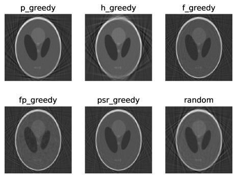
Figure 1: Reconstruction of Shepp-Logan phantom for different greedy methods.

Method	MSR error	MSI error	${\rm cond}_{2}(A_{K,\Lambda_{M}})$
no thinning	$5.8605\times 10^{-3}$		$1.2778\times 10^{10}$
$P$-greedy	$7.3435\times 10^{-3}$	$1.5072\times 10^{-4}$	$1.0924\times 10^{4}$
$h$-greedy	$1.1812\times 10^{-2}$	$5.4554\times 10^{-4}$	$8.5105\times 10^{4}$
$f$-greedy	$5.9693\times 10^{-3}$	$2.5043\times 10^{-6}$	$5.2886\times 10^{6}$
$f/P$-greedy	$6.0338\times 10^{-3}$	$1.4305\times 10^{-5}$	$2.4463\times 10^{7}$
psr-greedy	$5.2963\times 10^{-3}$	$5.0594\times 10^{-6}$	$7.031\times 10^{5}$
random	$8.32\times 10^{-3}$	$1.3848\times 10^{-4}$	$1.9706\times 10^{8}$

Table 1: Mean square errors, MSR and MSI, and condition numbers.

6 Acknowledgment

The authors acknowledge the support by the Deutsche Forschungsgemeinschaft (DFG) within the Research Training Group GRK 2583 „Modeling, Simulation and Optimization of Fluid Dynamic Applications“. Finally, we wish to thank Tizian Wenzel for several fruitful discussions.

References

- [1]
- [2] T. Aboiyar, E.H. Georgoulis, and A. Iske: Adaptive ADER methods using kernel-based polyharmonic spline WENO reconstruction. SIAM Journal on Scientific Computing 32 (6), 2010, 3251–3277.
-
[3]
M.D. Buhmann:
Radial Basis Functions.
Cambridge University Press, Cambridge, UK, 2003. - [4] S. De Marchi, A. Iske, and G. Santin: Image reconstruction from scattered Radon data by weighted positive definite kernel functions. Calcolo 55, 2018, 1–24.
- [5] S. De Marchi, R. Schaback, and H. Wendland: Near-optimal data-independent point locations for radial basis function interpolation. Advances in Computational Mathematics 23, 2005, 317–330.
- [6] R. DeVore, G. Petrova, and P. Wojtaszczyk: Greedy algorithms for reduced bases in Banach spaces. Constructive Approximation 37 (3), 2013, 455–466.
- [7] S. Dutta, M.W. Farthing, E. Perracchione, G. Savant, and M. Putti: A greedy non-intrusive reduced order model for shallow water equations. Journal of Computational Physics 439, 2021, 110378.
- [8] N. Dyn, M.S. Floater, and A. Iske: Adaptive thinning for bivariate scattered data. Journal of Computational and Applied Mathematics 145 (2), 505–517.
- [9] A. Iske: Reconstruction of functions from generalized Hermite-Birkhoff data. Series in Approximations and Decompositions 6, 1995, 257–264.
- [10] A. Iske: Approximation Theory and Algorithms for Data Analysis. Springer International Publishing, 2018.
- [11] A. Iske and T. Sonar: On the structure of function spaces in optimal recovery of point functionals for ENO-schemes by radial basis functions. Numerische Mathematik 74 (2), 1996, 177–201.
- [12] S. Müller: Komplexität und Stabilität von kernbasierten Rekonstruktionsmethoden. Dissertation, Georg-August-Universität Göttingen, 2009.
- [13] S. Müller and R. Schaback: A Newton basis for kernel spaces. Journal of Approximation Theory 161 (2), 2009, 645–655.
- [14] M. Pazouki and R. Schaback: Bases for kernel-based spaces. Journal of Computational and Applied Mathematics 236 (4), 2011, 575–588.
- [15] R. Schaback and H. Wendland: Adaptive greedy techniques for approximate solution of large RBF systems. Numerical Algorithms 24 (3), 2000, 239–254.
- [16] R. Schaback and J. Werner: Linearly constrained reconstruction of functions by kernels with applications to machine learning. Advances in Computational Mathematics 25, 2006, 237–258.
- [17] L.A. Shepp and B.F. Logan: The Fourier reconstruction of a head section. IEEE Transactions on Nuclear Science 21 (3), 1974, 21–43.
- [18] H. Wendland: Scattered Data Approximation. Cambridge University Press, Cambridge, UK, 2005.
- [19] T. Wenzel, G. Santin, and B. Haasdonk: Analysis of target data-dependent greedy kernel algorithms: convergence rates for -, - and -greedy. Constructive Approximation 57 (1), 2023, 45–74.
- [20] T. Wenzel, D. Winkle, G. Santin, and B. Haasdonk: Adaptive meshfree solution of linear partial differential equations with PDE-greedy kernel methods. arXiv preprint, arXiv:2207.13971, 2022.
- [21] Z. Wu: Hermite-Birkhoff interpolation of scattered data by radial basis functions. Approximation Theory Appl. 8, 1992, 1–10.