Emergent Interpretable Symbols and Content-Style Disentanglement via Variance-Invariance Constraints

Abstract

We contribute an unsupervised method that effectively learns from raw observation and disentangles its latent space into content and style representations. Unlike most disentanglement algorithms that rely on domain-specific labels and knowledge, our method is based on the insight of domain-general statistical differences between content and style — content varies more among different fragments within a sample but maintains an invariant vocabulary across data samples, whereas style remains relatively invariant within a sample but exhibits more significant variation across different samples. We integrate such inductive bias into an encoder-decoder architecture and name our method after V3 (variance-versus-invariance). Experimental results show that V3 generalizes across two distinct domains in different modalities, music audio and images of written digits, successfully learning pitch-timbre and digit-color disentanglements, respectively. Also, the disentanglement robustness significantly outperforms baseline unsupervised methods and is even comparable to supervised counterparts. Furthermore, symbolic-level interpretability emerges in the learned codebook of content, forging a near one-to-one alignment between machine representation and human knowledge .

1 Introduction

Learning abstract and symbolic representations is an essential part of human intelligence. Even without any label supervision, we humans can abstract rich observations with great variety into a category, and such capability generalizes across different domains and modalities. For example, we can effortlessly perceive a picture of a “cat” captured at any angle or set against any background, we can perceive the symbolic number “8” from an image irrespective of its color or writing style variations, and we can perceive an abstract pitch class “A” from an acoustic signal regardless of its timbre. These symbols form the fundamental vocabulary of our languages—be they natural, mathematical, or musical—and underpin effective and interpretable communication in everyday life.

Our goal is to emulate such abstraction capability using machine learning. We choose a content-style representation disentanglement approach as we believe that representation disentanglement offers a more complete picture of learning symbolic abstractions—concepts that matter more in communication, such as an “8” in a written phone number or a note pitch “A” in a folk song, are usually perceived as content, while the associated variations that often matter less in context, such as the written style of a digit or the singing style of a song, are perceived as style. In addition, content is usually symbolized and associated with rigid labels, as we need precise control over it during communication. E.g., to write “8” as “9” in a phone number or to sing an “A” as “B” in a performance can be a fatal error. In comparison, though style can also be described discretely, such as an “italic” writing or a “tenor” voice, a variation over it is usually much more tolerable.

In the machine-learning literature, significant progress has been made recently in content-style disentanglement for various tasks, including disentangling objects from backgrounds hong2023improving , characters from fonts liu2018multi ; xie2021dg , pitch from timbre lu2019play ; bonnici2022timbre , and phonemes from speaker identity qian2019autovc ; li2021starganv2 . However, most existing models rely heavily on domain-specific knowledge and require substantial supervision. The supervision forms can be explicit content or style labels liu2017unsupervised ; taigman2016unsupervised ; zhu2017unpaired ; park2020contrastive ; karras2019style ; choi2020stargan ; bonnici2022timbre ; patashnik2021styleclip ; kwon2022clipstyler , pre-trained content or style representations qian2020f0 ; qian2020unsupervised ; qian2019autovc , or paired data showcasing the same content rendered in different styles or vice versa isola2017image ; sangkloy2017scribbler . Additionally, the learned representations often lack interpretability at a symbolic level and do not align well with human perceptions zhang2021survey ; nauta2023anecdotal .

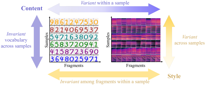
Figure 1: An illustration of the variance-versus-invariance constraints of content and style.

To address the aforementioned challenges and achieve more interpretable disentanglement in an unsupervised manner, we introduce V3 (variance-versus-invariance), a novel method to disentangle content and style by leveraging meta-level prior knowledge about their inherent statistical differences. As shown in Figure 1, our design principle is based on the observation that content and style display distinct patterns of variation—content undergoes frequent changes within different fragments of a sample yet maintains a consistent vocabulary across data samples, whereas style remains relatively stable within a sample but exhibits more significant variation across different samples.

In this paper, we adopt the vector-quantized autoencoder architecture and incorporate variance-versus-invariance constraints to guide the learning of latent representations that capture style-content distinctions. As for applications, we demonstrate that our method effectively generalizes across two distinct areas: disentangling pitches and timbres from musical data, and disentangling numbers and ink colors from images of handwritten digits. Experimental results show that our approach achieves more robust content-style disentanglement than baselines and is even comparable to supervised approaches. Moreover, symbolic-level interpretability emerges in a near one-to-one alignment between the vector-quantized codebook and human knowledge, an outcome not yet seen in previous studies. In summary, our contributions are as follows:

• Unsupervised content-style disentanglement: We introduce an unsupervised method that successfully learns to disentangle content and style representations without the need for paired data or explicit content and style labels.

• Emergence of interpretable symbols: Our innovative training objective fosters the development of interpretable content symbols that closely align with human knowledge.

• Generalizability of variance-vs-invariance constraints : V3 is a purely statistical method that relies only on meta-level inductive bias and does not require domain-specific assumptions typically necessary in visual or auditory data processing (such as a relation between foreground and background in the image domain or the relation between f0 and partials in the music domain).

2 Related Work

The content-style disentanglement as well as the related style transfer problem has been well explored in computer vision, especially in the context of image-to-image translation. Early works mostly require paired data of the same content with different styles isola2017image ; sangkloy2017scribbler , until the introduction of domain transfer networks that can learn style transfer functions without paired data zhu2017unpaired ; liu2017unsupervised ; taigman2016unsupervised ; bousmalis2017unsupervised ; park2020contrastive ; choi2018stargan ; choi2020stargan ; karras2019style ; xie2022unsupervised ; xie2022multi . Although these methods are unsupervised in the sense that they do not require paired data, they still require concrete labels of styles to identify source and target domains, and there are no fully interpretable representations of either content or style.

A similar trajectory of research has also been followed in other domains including speech qian2019autovc ; kameoka2018stargan ; kaneko2019stargan ; wu2023large and music huang2018timbretron ; bonnici2022timbre ; lu2019play ; lin2023content ; zhang2024musicmagus ; lin2021unified ; engel2020self . To mitigate the requirement for supervision, some methods utilize domain-specific knowledge and have achieved better disentanglement results, including X-vectors of speakers qian2019autovc ; qian2020f0 , the close relation between fundamental frequency and content in audio qian2020f0 ; qian2020unsupervised , or pre-defined style or content representations yangdeep ; wang2020learning ; wang2022audio . Pure unsupervised learning for content and style disentanglement has not been well explored. Notable attempts include mutual information-based methods such as InfoGAN and mutual information neural estimation (MINE) chen2016infogan ; belghazi2018mutual ; poole2019variational ; tjandra2020unsupervised , and low-dimensional representation learning with physical symmetry liu2023learning . But these methods often suffer from the training stability issue or have to follow a low-dimensionality setup.

A technique often associated with learned content is vector quantization (VQ) van2017neural . Recent efforts have built language models on top of VQ codes for long-term generation, indicating the association between VQ codebook and the underlying information content yan2021videogpt ; tan2021vimpac ; copet2024simple ; garcia2023vampnet ; tjandra2020unsupervised ; tjandra2020transformer ; vali2023interpretable . A noticeable characteristic of these studies is the use of large codebooks, which limits the interpretability of representations. We borrow the idea of a small codebook size from categorical representations chen2016infogan ; ji2019invariant , targeting a more concise and unified content code across different styles, while keeping the high-dimensional nature of VQ representations.

3 Methodology

Considering a dataset consisting of $N$ data samples, where each sample contains $L$ fragments. We aim to learn each fragment’s content and style representation with the inductive bias illustrated in Figure 1. Intuitively, the fragments within each data sample have a relatively frequently-changing content and a relatively stable style. For different data samples, the style exhibits significant variations and their content more or less keeps a consistent vocabulary. In this paper, we focus on two tasks: 1) learning pitch (content) and timbre (style) representations from audio spectrograms where each sample contains several note fragments, and 2) learning digits (content) and ink colors (style) representations from images of written digit strings where each fragment is a written number.

3.1 Model Architecture

The model architecture of V3 is illustrated in Figure 2. Let ${\bm{X}}=\{{\bm{x}}_{ij}\}_{N\times L}$ be the dataset, where ${\bm{x}}_{ij}$ corresponds to the $j$-th fragment of the $i$-th sample. We use an autoencoder architecture to learn the representations of ${\bm{x}}_{ij}$. The encoder encodes the input data ${\bm{x}}_{ij}$ to the latent space, which is split into to ${\bm{z}}_{ij}^{\mathrm{c}}$ and ${\bm{z}}_{ij}^{\mathrm{s}}$. We use vector quantization as the dictionary learning method for content. Every content representation ${\bm{z}}_{ij}^{\mathrm{c}}$ is quantized to the nearest atom in a codebook of size $K$ as $\tilde{{\bm{z}}}_{ij}^{\mathrm{c}}$. The decoder concatenates $\tilde{{\bm{z}}}_{ij}^{\mathrm{c}}$ and ${\bm{z}}_{ij}^{\mathrm{s}}$ and reconstructs the fragment $\hat{{\bm{x}}}_{ij}$. The overall loss function is the weighted sum of three terms:

$$\mathcal{L}=\mathcal{L}_{\mathrm{rec}}+\alpha\mathcal{L}_{\mathrm{vq}}+\beta\mathcal{L}_{\mathrm{V3}}\text{.}$$ (1)

Here, $\mathcal{L}_{\text{rec}}$ is the reconstruction loss of ${\bm{X}}$ and $\mathcal{L}_{\text{vq}}$ is the VQ commit loss van2017neural :

$$\mathcal{L}_{\mathrm{rec}} =\frac{1}{N\times L}\sum_{i=1}^{N}\sum_{j=1}^{L}\|{\bm{x}}_{ij}-\hat{{\bm{x}}}_{ij}\|_{2}\text{,}$$ (2)

$$\mathcal{L}_{\mathrm{vq}} =\frac{1}{N\times L}\sum_{i=1}^{N}\sum_{j=1}^{L}\|{\bm{z}}_{ij}^{\mathrm{c}}-\mathrm{sg}(\tilde{{\bm{z}}}_{ij}^{\mathrm{c}})\|_{2}\text{,}$$ (3)

where $\mathrm{sg}(\cdot)$ is the stop gradient operation of the straight-through optimization. The final term $\mathcal{L}_{\mathrm{V3}}$ is the proposed regularization method to ensure unsupervised content-style disentanglement, which we introduce in the rest part of this section. (For more details of the model architecture and data representations, we refer the readers to the appendix.)

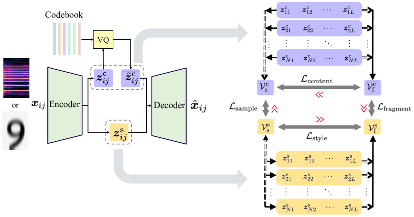
Figure 2: The model architecture of V3. Left: The autoencoder has two branches for content and style respectively, where the content branch has a VQ layer at the encoder output. Right: the V3 constraints, where double-dashed arrows represent measuring the variability by $\nu_{k}(\cdot)$, and solid arrows represent taking the average.

3.2 Variability Statistics

We define four statistics to measure the degree of variability in accordance with the four edges of Figure 1. These statistics are based on a backbone variability measurement $\nu_{k}(\cdot)$, where $k$ represents the dimension along which variability is computed. In this paper, we define $\nu_{k}(\cdot)$ as the mean pairwise distance (MPD). Formally, for a vector ${\bm{z}}$ of length $D$,

$$\nu_{i=1}^{D}({\bm{z}}_{i}):=\mathrm{MPD}_{i=1}^{D}({\bm{z}}_{i})=\frac{1}{D(D-1)}\sum_{i=1}^{D}\sum_{j=1,j\neq i}^{D}\|{\bm{z}}_{i}-{\bm{z}}_{j}\|_{2}\text{.}$$ (4)

The motivation for using MPD is that it is more sensitive to multi-peak distributions than standard deviation, which is preferred when learning diverse content symbols in a sample. We compare different choices of $\nu_{k}(\cdot)$ in Section 4.1.

Content variability within a sample ($\mathcal{V}_{\mathrm{f}}^{\mathrm{c}}$). We first compute the variability of content along the fragment axis and take the average along the sample axis. The value is the average of content codes before and after vector quantization:

$$\mathcal{V}_{\mathrm{f}}^{\mathrm{c}}=\frac{1}{2N}\sum_{i=1}^{N}\nu_{j=1}^{L}({\bm{z}}^{\mathrm{c}}_{ij})+\frac{1}{2N}\sum_{i=1}^{N}\nu_{j=1}^{L}(\tilde{{\bm{z}}}^{\mathrm{c}}_{ij})\text{.}$$ (5)

Content variability across samples ($\mathcal{V}_{\mathrm{s}}^{\mathrm{c}}$). Theoretically, we aim to measure the consistency of codebook usage distribution along the sample axis, which is not differentiable. In practice, we compute the center of the content code along the fragment axis and measure the variability of the centers along the sample axis. It serves as a proxy of codebook utilization. Also, we consider both the original content codes (before and after vector quantization):

$$\mathcal{V}_{\mathrm{s}}^{\mathrm{c}}=\frac{1}{2}\nu_{i=1}^{N}\bigl{(}\frac{1}{L}\sum_{j=1}^{L}{\bm{z}}^{\mathrm{c}}_{ij}\bigr{)}+\frac{1}{2}\nu_{i=1}^{N}\bigl{(}\frac{1}{L}\sum_{j=1}^{L}\tilde{{\bm{z}}}^{\mathrm{c}}_{ij}\bigr{)}\text{.}$$ (6)

Style variability within a sample ($\mathcal{V}_{\mathrm{f}}^{\mathrm{s}}$). We compute the variability of style representations among fragments and take its mean across all samples:

$$\mathcal{V}_{\mathrm{f}}^{\mathrm{s}}=\frac{1}{N}\sum_{i=1}^{N}\nu_{j=1}^{L}({\bm{z}}^{\mathrm{s}}_{ij})\text{.}$$ (7)

Style variability across samples ($\mathcal{V}_{\mathrm{s}}^{\mathrm{s}}$). We compute the average style representation along the fragment axis and measure its variability along the sample axis:

$$\mathcal{V}_{\mathrm{s}}^{\mathrm{s}}=\nu_{i=1}^{N}\bigl{(}\frac{1}{L}\sum_{j=1}^{L}{\bm{z}}^{\mathrm{s}}_{ij}\bigr{)}\text{.}$$ (8)

3.3 Variance-Versus-Invariance (V3) Constraints

With the variability statistics, we can formalize the general relationship between content and style along the sample or fragment axis:

• Content should be more variable within samples than across samples, i.e., $\mathcal{V}_{\mathrm{f}}^{\mathrm{c}}\gg\mathcal{V}_{\mathrm{s}}^{\mathrm{c}}$.

• Style should be more variable across samples than within samples, i.e., $\mathcal{V}_{\mathrm{s}}^{\mathrm{s}}\gg\mathcal{V}_{\mathrm{s}}^{\mathrm{f}}$.

• Within a sample, content should be more variable than style, i.e, $\mathcal{V}_{\mathrm{f}}^{\mathrm{c}}\gg\mathcal{V}_{\mathrm{f}}^{\mathrm{s}}$.

• Across samples, style should be more variable than content, i.e., $\mathcal{V}_{\mathrm{s}}^{\mathrm{s}}\gg\mathcal{V}_{\mathrm{s}}^{\mathrm{c}}$.

We quantify the above contrasts as regularization terms, using the hinge function to cut off gradient back-propagation when the ratio between two variability statistics reaches a certain threshold $r>1$, which stands for relativity bardes2022vicreg :

$$\mathcal{L}_{\mathrm{content}} =\max(0,1-\frac{\mathcal{V}_{\mathrm{f}}^{\mathrm{c}}}{r\cdot\mathcal{V}_{\mathrm{s}}^{\mathrm{c}}})\text{,}\quad\text{(}\mathcal{V}_{\mathrm{f}}^{\mathrm{c}}\gg\mathcal{V}_{\mathrm{s}}^{\mathrm{c}}\text{)}$$ (9)

$$\mathcal{L}_{\mathrm{style}} =\max(0,1-\frac{\mathcal{V}_{\mathrm{s}}^{\mathrm{s}}}{r\cdot\mathcal{V}_{\mathrm{f}}^{\mathrm{s}}})\text{,}\quad\text{(}\mathcal{V}_{\mathrm{s}}^{\mathrm{s}}\gg\mathcal{V}_{\mathrm{f}}^{\mathrm{s}}\text{)}$$ (10)

$$\mathcal{L}_{\mathrm{fragment}} =\max(0,1-\frac{\mathcal{V}_{\mathrm{f}}^{\mathrm{c}}}{r\cdot\mathcal{V}_{\mathrm{f}}^{\mathrm{s}}})\text{,}\quad\text{(}\mathcal{V}_{\mathrm{f}}^{\mathrm{c}}\gg\mathcal{V}_{\mathrm{f}}^{\mathrm{s}}\text{)}$$ (11)

$$\mathcal{L}_{\mathrm{sample}} =\max(0,1-\frac{\mathcal{V}_{\mathrm{s}}^{\mathrm{s}}}{r\cdot\mathcal{V}_{\mathrm{s}}^{\mathrm{c}}})\text{.}\quad\text{(}\mathcal{V}_{\mathrm{s}}^{\mathrm{s}}\gg\mathcal{V}_{\mathrm{s}}^{\mathrm{c}}\text{)}$$ (12)

We obtain the V3 regularization term (used in Equation 1) by summing up the four terms:

$$\mathcal{L}_{\mathrm{V3}}=\mathcal{L}_{\mathrm{content}}+\mathcal{L}_{\mathrm{style}}+\mathcal{L}_{\mathrm{fragment}}+\mathcal{L}_{\mathrm{sample}}\text{.}$$ (13)

4 Experiments

We evaluate V3 on two tasks of different domains to demonstrate its effectiveness and generalizability. The first task is learning pitches and timbres from monophonic music audio (Section 4.2), and the second task is learning digits and ink colors from written digit strings (Section 4.3). The highlight of this section is that V3 effectively learns disentangled representations of content and style, and the discrete content representations align well with human knowledge.

4.1 Experiment Setup

Baselines: We compare V3 with two unsupervised baselines: 1) an unsupervised content-style disentanglement based on MINE tjandra2020unsupervised , and 2) a 2-branch autoencoder similar to our architecture choice, but trained with the cycle consistency loss after decoding and encoding shuffled combinations of $\tilde{{\bm{z}}^{\mathrm{c}}}$ and ${\bm{z}}^{\mathrm{s}}$ zhu2017unpaired .

Additionally, we compare with two supervised learning methods. The first one is a weakly supervised method provided with content labels, in which the model is trained to predict the correct content labels from ${\bm{z}}_{ij}^{\mathrm{c}}$ as a replacement of the VQ layer, and the decoder is trained to reconstruct inputs from ${\bm{z}}_{ij}^{\mathrm{s}}$ and ground truth content labels yangdeep ; wang2020learning . The second one is a fully supervised method provided with both content and style labels, in which the model learns to predict both content and style from their latent representations. We provide further details of the baselines in the appendix.

Table 1: Evaluation of pitch and timbre disentanglement and pitch codebook interpretability. The metrics are defined in Section 4.1.

Method	$K$	Content		Style		Codebook Interpretability
		PR-AUC $\uparrow$	Best F1 $\uparrow$	PR-AUC $\uparrow$	Best F1 $\uparrow$	Accuracy $\uparrow$	$\sigma$ $\downarrow$
V3	$12$	0.904	0.904	0.879	0.879	0.999	0.001
	$24$	0.794	0.805	0.704	0.723	0.929	0.022
	$48$	0.723	0.752	0.757	0.807	0.901	0.045
MINE-based	$12$	0.085	0.147	0.108	0.152	0.138	0.038
	$24$	0.092	0.153	0.160	0.189	0.294	0.089
	$48$	0.109	0.165	0.186	0.206	0.239	0.006
Cycle loss	$12$	0.083	0.146	0.113	0.164	0.275	0.104
	$24$	0.082	0.145	0.151	0.221	0.285	0.119
	$48$	0.084	0.150	0.200	0.241	0.182	0.062
Weakly supervised	$12$	0.730	0.759	0.704	0.725	0.999	0.001
Fully supervised	$12$	0.904	0.904	0.905	0.904	1.000	0.000

Ablation: For ablation, we experiment with another type of variability measurement $\nu_{k}(\cdot)$, which is standard deviation (SD). Besides, we train four ablated versions of V3, each without one of the four regularization terms defined in Equation 9-12 to test its robustness.

Choice of $K$: In reality, we do not always know the real number of content labels, and there is a ubiquity of vocabulary redundancy in human symbol systems, including language. This fact marks an improvement of our method from classification-based methods that we do not need to know the real value of $K$ to perform well. To fully illustrate this, we test all unsupervised methods under three different $K$ settings, which stand for different levels of codebook redundancy.

Evaluation Metrics: We evaluate the models both quantitatively and qualitatively, from two aspects:

• The content and style disentanglement ability in latent space. For numerical results, we conduct a retrieval experiment to examine the nearest neighbors of every input ${\bm{z}}^{\mathrm{c}}$ and ${\bm{z}}^{\mathrm{s}}$ using ground truth content and style labels, evaluated by the area under the precision-recall curve (PR-AUC) and the best F1 score.

• The codebook interpretability. We plot the confusion matrix of codebooks by aligning each codebook atom to one content label. Quantitatively, we compute the codebook accuracy by counting the correct assignments, and the standard deviation ($\sigma$) that shows the degree of disagreement of codebook assignments among different styles. A good codebook that aligns well with human knowledge should have a clean stair-like confusion matrix, with a high accuracy and a low $\sigma$ value.

Figure 3: t-SNE visualization of the learned pitch (content) and timbre (style) representations. The first row visualizes pitch representations before quantization. The style labels in the second row show the names of instruments.

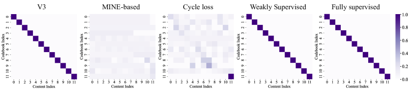
Figure 4: Confusion matrices of learned codebooks for pitches. The horizontal axes show pitch labels from “C” to “B”, and the vertical axes show codebook atoms aligned with pitch labels.

4.2 Learning Pitches and Timbres from Music

Dataset: We synthesize a dataset consisting of monophonic music audio of 12 different instruments playing 12 different pitches in an octave from C4 to B4. Every pitch is played for one second one by one with a random velocity between 80 and 120. We synthesize the audio at 16kHz for each instrument and further diversify the notes by adding a random amplitude envelope to each note. The audio files are then normalized and processed to magnitude spectrograms.

Experiment Results: We present the quantitive results on the test set in Table 1. We see that V3 exhibits superior performance in terms of both representation disentanglement and codebook interpretability compared to the unsupervised baselines, regardless of the codebook size $K$. It is worth noticing that V3 also outperforms the weakly supervised baseline in the retrieval of timbre (style) representation task, which indicates that V3 learns better-disentangled timbre representations containing less pitch information.

Figure 3 further shows the t-SNE visualization of the pitch and timbre representations by different methods when $K=12$, demonstrating that V3 learns representations with clean clustering comparable to supervised methods. Figure 4 shows the confusion matrices of content codebooks of classification results when $K=12$. Among unsupervised methods, V3 achieves the clearest one-to-one mapping from 12 codebook vocabularies to 12 pitches, illustrating the strong symbolic-level interpretability of learned contents.

Table 2: Ablation of different V3 settings on learning pitches and timbres.

Method	$K$	Content		Style		Codebook Interpretability
		PR-AUC $\uparrow$	Best F1 $\uparrow$	PR-AUC $\uparrow$	Best F1 $\uparrow$	Accuracy $\uparrow$	$\sigma$ $\downarrow$
V3	$12$	0.904	0.904	0.879	0.879	0.999	0.001
V3 ($\nu_{k}=\mathrm{SD}$)	$12$	0.138	0.183	0.241	0.330	0.333	0.101
V3 (w/o $\mathcal{L}_{\mathrm{content}}$)	$12$	0.210	0.285	0.677	0.696	0.436	0.034
V3 (w/o $\mathcal{L}_{\mathrm{style}}$)	$12$	0.899	0.903	0.810	0.817	0.999	0.001
V3 (w/o $\mathcal{L}_{\mathrm{fragment}}$)	$12$	0.276	0.360	0.543	0.562	0.455	0.074
V3 (w/o $\mathcal{L}_{\mathrm{sample}}$)	$12$	0.903	0.903	0.509	0.570	0.997	0.001

Table 3: Evaluation of digit and color disentanglement and digit code book interpretability. The metrics are defined in Section 4.1.

Method	$K$	Content		Style		Codebook Interpretability
		PR-AUC $\uparrow$	Best F1 $\uparrow$	PR-AUC $\uparrow$	Best F1 $\uparrow$	Accuracy $\uparrow$	$\sigma$ $\downarrow$
V3	$10$	0.734	0.793	0.967	0.937	0.892	0.006
	$20$	0.938	0.902	0.945	0.916	0.997	0.018
	$40$	0.843	0.824	0.953	0.930	1.000	0.045
MINE-based	$10$	0.218	0.308	0.355	0.386	0.409	0.081
	$20$	0.117	0.186	0.226	0.335	0.256	0.098
	$40$	0.134	0.192	0.268	0.363	0.506	0.062
Cycle loss	$10$	0.143	0.184	0.244	0.288	0.710	0.037
	$20$	0.560	0.634	0.237	0.278	0.896	0.043
	$40$	0.507	0.587	0.219	0.257	1.000	0.041
Weakly supervised	$10$	0.952	0.951	0.575	0.570	1.000	0.000
Fully supervised	$10$	0.952	0.951	0.962	0.915	1.000	0.000

Table 4: Ablation of V3 settings on learning digits and colors.

Method	$K$	Content		Style		Codebook Interpretability
		PR-AUC $\uparrow$	Best F1 $\uparrow$	PR-AUC $\uparrow$	Best F1 $\uparrow$	Accuracy $\uparrow$	$\sigma$ $\downarrow$
V3	$10$	0.734	0.793	0.967	0.937	0.892	0.006
V3 ($\nu_{k}=\mathrm{SD}$)	$10$	0.427	0.532	0.497	0.518	0.648	0.051
V3 (w/o $\mathcal{L}_{\text{content}}$)	$10$	0.453	0.525	0.926	0.890	0.586	0.051
V3 (w/o $\mathcal{L}_{\text{style}}$)	$10$	0.634	0.675	0.918	0.888	0.726	0.035
V3 (w/o $\mathcal{L}_{\text{fragment}}$)	$10$	0.977	0.993	0.953	0.909	1.000	0.000
V3 (w/o $\mathcal{L}_{\text{sample}}$)	$10$	0.480	0.578	0.942	0.894	0.653	0.024

Ablation Study: We compare the performances of V3 and its variants in Table 2. It can be seen that $\nu_{k}=\mathrm{SD}$ does not work as well as $\nu_{k}=\mathrm{MPD}$ due to its weakness in constraining multi-peak content distributions within samples. It is also worth noting that V3 performs fairly well even when discarding $\mathcal{L}_{\mathrm{style}}$ or $\mathcal{L}_{\mathrm{sample}}$. In both cases, we observe a decrease in the discarded loss even if we do not explicitly optimize for it. We suspect this is due to the robustness of V3 constraints as reflected in the symmetric relationships among the four losses—we can enforce three relations, and the fourth one may fall into the right place. However, in practice, it is difficult to tell the “free relation” beforehand as it is also related to detailed content and style variations in specific domains.

4.3 Learning Digits and Colors from Written Digit Strings

Dataset: We synthesize an image dataset of written digit strings on light backgrounds using all 10 digits and 8 different ink colors. The order of digits is random. All images are diversified with Gaussian noises, random blur, and foreground and background color jitters. More details about the dataset can be found in the appendix.

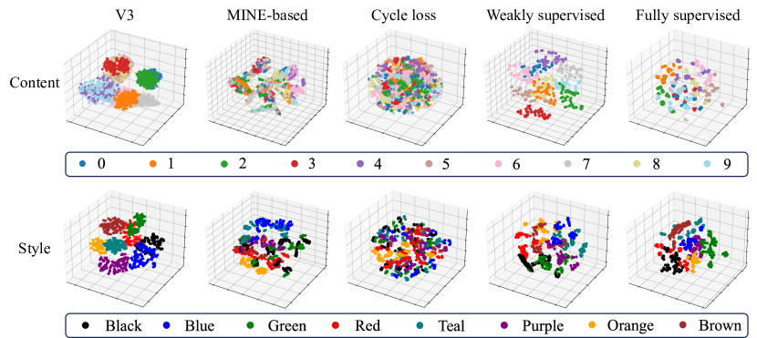
Figure 5: t-SNE visualization of the learned digit (content) and color (style) representations. The first row shows content representations before quantization, and the second row’s visualizations use the same colors as the digits are written.

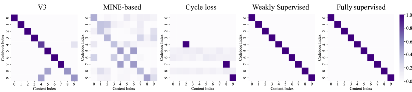
Figure 6: Confusion matrices of learned codebooks for digits. The horizontal axes show digit labels from “0” to “9”, and the vertical axes show codebook atoms aligned with digit labels.

Experiment Results: The quantitive results can be seen in Table 3. Similar to the music task, V3 performs the best considering both representation disentanglement and codebook interpretability. Even though some unsupervised baselines also achieve a high codebook accuracy at large $K$ values, they fall behind in terms of latent space retrieval, especially in style. We visualize the latent representations in Figure 5, and compare the confusion matrices in Figure 6 for intuitive understanding.

Ablation Study: Table 4 shows the ablation results of V3 on the digit string dataset. The inferior performance of $\nu_{k}=\mathrm{SD}$ supports our assumption of its weakness in capturing multi-peak high-dimensional distributions. We observe that V3 trained without $\mathcal{L}_{\mathrm{fragment}}$ achieves the best codebook interpretability. Referring to the ablation in section 4.2, it is conceivable that a three-loss target can sometimes also satisfy the four constraints as defined in V3, and the optimal value for hyperparameters r and $\beta$ may differ by datasets, which marks a possible direction for future improvements.

5 Limitation

We have identified several limitations in our V3 method that necessitate further investigation. First, while V3 achieves good disentanglement and symbolic interpretability, it is not flawless — samples of different contents (say images of “8" and “9") may sometimes be projected into the same latent code. Inspired by human learning, which effectively integrates both mode-1 and mode-2 cognitive processes, we aim to enhance V3 by incorporating certain feedback or reinforcement. This adaptation could also facilitate the application of V3 to more complex domains such as general image or video. Additionally, V3 is currently optimized to disentangle content and style from data samples that include defined fragments. Extending this capability to unsegmented data, such as continuous audio, represents a significant area for future development. Furthermore, V3 assumes that content elements do not overlap, which does not hold in cases of polyphonic music or mixed audio. Addressing this challenge will require a more sophisticated approach that considers the hierarchical nature of content.

6 Conclusion

In conclusion, we contributed an unsupervised content-style disentanglement method V3, which leads to an emergence of symbolic-level interpretability of the learned latent space. V3’s inductive bias is domain-general, intuitive, and concise, solely based on the meta-level insight of the statistical difference between content and style, i.e., their distinct variance-invariance patterns reflected both within and across data samples. Experiments show that V3 not only outperforms the baselines in terms of both disentanglement and latent space interpretability but also achieves comparable results with supervised models under a similar auto-encoding architecture. Moreover, the effectiveness of V3 generalizes across two distinct domains: music audio and written digits. For contents, the VQ codebooks learned by V3 have a near one-to-one alignment with human knowledge of music scales (the 12 semitones from C to B) and numbers (the 10 digits from 0 to 9). For style, V3 learns a latent space where different colors or instruments naturally form clusters without any label supervision or even a KL regularization that is usually needed for a well-structured latent space.

References

- (1) Ziming Hong, Zhenyi Wang, Li Shen, Yu Yao, Zhuo Huang, Shiming Chen, Chuanwu Yang, Mingming Gong, and Tongliang Liu. Improving non-transferable representation learning by harnessing content and style. In The Twelfth International Conference on Learning Representations, 2023.
- (2) Yang Liu, Zhaowen Wang, Hailin Jin, and Ian Wassell. Multi-task adversarial network for disentangled feature learning. In Proceedings of the IEEE Conference on Computer Vision and Pattern Recognition, pages 3743–3751, 2018.
- (3) Yangchen Xie, Xinyuan Chen, Li Sun, and Yue Lu. Dg-font: Deformable generative networks for unsupervised font generation. In Proceedings of the IEEE/CVF conference on computer vision and pattern recognition, pages 5130–5140, 2021.
- (4) Chien-Yu Lu, Min-Xin Xue, Chia-Che Chang, Che-Rung Lee, and Li Su. Play as you like: Timbre-enhanced multi-modal music style transfer. In Proceedings of the aaai conference on artificial intelligence, volume 33, pages 1061–1068, 2019.
- (5) Russell Sammut Bonnici, Martin Benning, and Charalampos Saitis. Timbre transfer with variational auto encoding and cycle-consistent adversarial networks. In 2022 International Joint Conference on Neural Networks (IJCNN), pages 1–8. IEEE, 2022.
- (6) Kaizhi Qian, Yang Zhang, Shiyu Chang, Xuesong Yang, and Mark Hasegawa-Johnson. Autovc: Zero-shot voice style transfer with only autoencoder loss. In International Conference on Machine Learning, pages 5210–5219. PMLR, 2019.
- (7) Yinghao Aaron Li, Ali Zare, and Nima Mesgarani. Starganv2-vc: A diverse, unsupervised, non-parallel framework for natural-sounding voice conversion. arXiv preprint arXiv:2107.10394, 2021.
- (8) Ming-Yu Liu, Thomas Breuel, and Jan Kautz. Unsupervised image-to-image translation networks. Advances in neural information processing systems, 30, 2017.
- (9) Yaniv Taigman, Adam Polyak, and Lior Wolf. Unsupervised cross-domain image generation. arXiv preprint arXiv:1611.02200, 2016.
- (10) Jun-Yan Zhu, Taesung Park, Phillip Isola, and Alexei A Efros. Unpaired image-to-image translation using cycle-consistent adversarial networks. In Proceedings of the IEEE international conference on computer vision, pages 2223–2232, 2017.
- (11) Taesung Park, Alexei A Efros, Richard Zhang, and Jun-Yan Zhu. Contrastive learning for unpaired image-to-image translation. In Computer Vision–ECCV 2020: 16th European Conference, Glasgow, UK, August 23–28, 2020, Proceedings, Part IX 16, pages 319–345. Springer, 2020.
- (12) Tero Karras, Samuli Laine, and Timo Aila. A style-based generator architecture for generative adversarial networks. In Proceedings of the IEEE/CVF conference on computer vision and pattern recognition, pages 4401–4410, 2019.
- (13) Yunjey Choi, Youngjung Uh, Jaejun Yoo, and Jung-Woo Ha. Stargan v2: Diverse image synthesis for multiple domains. In Proceedings of the IEEE/CVF conference on computer vision and pattern recognition, pages 8188–8197, 2020.
- (14) Or Patashnik, Zongze Wu, Eli Shechtman, Daniel Cohen-Or, and Dani Lischinski. Styleclip: Text-driven manipulation of stylegan imagery. In Proceedings of the IEEE/CVF international conference on computer vision, pages 2085–2094, 2021.
- (15) Gihyun Kwon and Jong Chul Ye. Clipstyler: Image style transfer with a single text condition. In Proceedings of the IEEE/CVF Conference on Computer Vision and Pattern Recognition, pages 18062–18071, 2022.
- (16) Kaizhi Qian, Zeyu Jin, Mark Hasegawa-Johnson, and Gautham J Mysore. F0-consistent many-to-many non-parallel voice conversion via conditional autoencoder. In ICASSP 2020-2020 IEEE International Conference on Acoustics, Speech and Signal Processing (ICASSP), pages 6284–6288. IEEE, 2020.
- (17) Kaizhi Qian, Yang Zhang, Shiyu Chang, Mark Hasegawa-Johnson, and David Cox. Unsupervised speech decomposition via triple information bottleneck. In International Conference on Machine Learning, pages 7836–7846. PMLR, 2020.
- (18) Phillip Isola, Jun-Yan Zhu, Tinghui Zhou, and Alexei A Efros. Image-to-image translation with conditional adversarial networks. In Proceedings of the IEEE conference on computer vision and pattern recognition, pages 1125–1134, 2017.
- (19) Patsorn Sangkloy, Jingwan Lu, Chen Fang, Fisher Yu, and James Hays. Scribbler: Controlling deep image synthesis with sketch and color. In Proceedings of the IEEE conference on computer vision and pattern recognition, pages 5400–5409, 2017.
- (20) Yu Zhang, Peter Tiňo, Aleš Leonardis, and Ke Tang. A survey on neural network interpretability. IEEE Transactions on Emerging Topics in Computational Intelligence, 5(5):726–742, 2021.
- (21) Meike Nauta, Jan Trienes, Shreyasi Pathak, Elisa Nguyen, Michelle Peters, Yasmin Schmitt, Jörg Schlötterer, Maurice van Keulen, and Christin Seifert. From anecdotal evidence to quantitative evaluation methods: A systematic review on evaluating explainable ai. ACM Computing Surveys, 55(13s):1–42, 2023.
- (22) Konstantinos Bousmalis, Nathan Silberman, David Dohan, Dumitru Erhan, and Dilip Krishnan. Unsupervised pixel-level domain adaptation with generative adversarial networks. In Proceedings of the IEEE conference on computer vision and pattern recognition, pages 3722–3731, 2017.
- (23) Yunjey Choi, Minje Choi, Munyoung Kim, Jung-Woo Ha, Sunghun Kim, and Jaegul Choo. Stargan: Unified generative adversarial networks for multi-domain image-to-image translation. In Proceedings of the IEEE conference on computer vision and pattern recognition, pages 8789–8797, 2018.
- (24) Shaoan Xie, Qirong Ho, and Kun Zhang. Unsupervised image-to-image translation with density changing regularization. Advances in Neural Information Processing Systems, 35:28545–28558, 2022.
- (25) Shaoan Xie, Lingjing Kong, Mingming Gong, and Kun Zhang. Multi-domain image generation and translation with identifiability guarantees. In The Eleventh International Conference on Learning Representations, 2022.
- (26) Hirokazu Kameoka, Takuhiro Kaneko, Kou Tanaka, and Nobukatsu Hojo. Stargan-vc: Non-parallel many-to-many voice conversion using star generative adversarial networks. In 2018 IEEE Spoken Language Technology Workshop (SLT), pages 266–273. IEEE, 2018.
- (27) Takuhiro Kaneko, Hirokazu Kameoka, Kou Tanaka, and Nobukatsu Hojo. Stargan-vc2: Rethinking conditional methods for stargan-based voice conversion. arXiv preprint arXiv:1907.12279, 2019.
- (28) Yusong Wu, Ke Chen, Tianyu Zhang, Yuchen Hui, Taylor Berg-Kirkpatrick, and Shlomo Dubnov. Large-scale contrastive language-audio pretraining with feature fusion and keyword-to-caption augmentation. In ICASSP 2023-2023 IEEE International Conference on Acoustics, Speech and Signal Processing (ICASSP), pages 1–5. IEEE, 2023.
- (29) Sicong Huang, Qiyang Li, Cem Anil, Xuchan Bao, Sageev Oore, and Roger B Grosse. Timbretron: A wavenet (cyclegan (cqt (audio))) pipeline for musical timbre transfer. arXiv preprint arXiv:1811.09620, 2018.
- (30) Liwei Lin, Gus Xia, Junyan Jiang, and Yixiao Zhang. Content-based controls for music large language modeling. arXiv preprint arXiv:2310.17162, 2023.
- (31) Yixiao Zhang, Yukara Ikemiya, Gus Xia, Naoki Murata, Marco Martínez, Wei-Hsiang Liao, Yuki Mitsufuji, and Simon Dixon. Musicmagus: Zero-shot text-to-music editing via diffusion models. arXiv preprint arXiv:2402.06178, 2024.
- (32) Liwei Lin, Qiuqiang Kong, Junyan Jiang, and Gus Xia. A unified model for zero-shot music source separation, transcription and synthesis. arXiv preprint arXiv:2108.03456, 2021.
- (33) Jesse Engel, Rigel Swavely, Lamtharn Hanoi Hantrakul, Adam Roberts, and Curtis Hawthorne. Self-supervised pitch detection by inverse audio synthesis. In ICML 2020 Workshop on Self-supervision in Audio and Speech, 2020.
- (34) Ruihan Yang, Dingsu Wang, Ziyu Wang, Tianyao Chen, Junyan Jiang, and Gus Xia. Deep music analogy via latent representation disentanglement. In Proceedings of 230st International Conference on Music Information Retrieval (ISMIR), 2019.
- (35) Ziyu Wang, Dingsu Wang, Yixiao Zhang, and Gus Xia. Learning interpretable representation for controllable polyphonic music generation. In Proceedings of 21st International Conference on Music Information Retrieval (ISMIR), 2020.
- (36) Ziyu Wang, Dejing Xu, Gus Xia, and Ying Shan. Audio-to-symbolic arrangement via cross-modal music representation learning. In ICASSP 2022-2022 IEEE International Conference on Acoustics, Speech and Signal Processing (ICASSP), pages 181–185. IEEE, 2022.
- (37) Xi Chen, Yan Duan, Rein Houthooft, John Schulman, Ilya Sutskever, and Pieter Abbeel. Infogan: Interpretable representation learning by information maximizing generative adversarial nets. Advances in neural information processing systems, 29, 2016.
- (38) Mohamed Ishmael Belghazi, Aristide Baratin, Sai Rajeshwar, Sherjil Ozair, Yoshua Bengio, Aaron Courville, and Devon Hjelm. Mutual information neural estimation. In International conference on machine learning, pages 531–540. PMLR, 2018.
- (39) Ben Poole, Sherjil Ozair, Aaron Van Den Oord, Alex Alemi, and George Tucker. On variational bounds of mutual information. In International Conference on Machine Learning, pages 5171–5180. PMLR, 2019.
- (40) Andros Tjandra, Ruoming Pang, Yu Zhang, and Shigeki Karita. Unsupervised learning of disentangled speech content and style representation. arXiv preprint arXiv:2010.12973, 2020.
- (41) Xuanjie Liu, Daniel Chin, Yichen Huang, and Gus Xia. Learning interpretable low-dimensional representation via physical symmetry. arXiv preprint arXiv:2302.10890, 2023.
- (42) Aaron Van Den Oord, Oriol Vinyals, et al. Neural discrete representation learning. Advances in neural information processing systems, 30, 2017.
- (43) Wilson Yan, Yunzhi Zhang, Pieter Abbeel, and Aravind Srinivas. Videogpt: Video generation using vq-vae and transformers. arXiv preprint arXiv:2104.10157, 2021.
- (44) Hao Tan, Jie Lei, Thomas Wolf, and Mohit Bansal. Vimpac: Video pre-training via masked token prediction and contrastive learning. arXiv preprint arXiv:2106.11250, 2021.
- (45) Jade Copet, Felix Kreuk, Itai Gat, Tal Remez, David Kant, Gabriel Synnaeve, Yossi Adi, and Alexandre Défossez. Simple and controllable music generation. Advances in Neural Information Processing Systems, 36, 2024.
- (46) Hugo Flores Garcia, Prem Seetharaman, Rithesh Kumar, and Bryan Pardo. Vampnet: Music generation via masked acoustic token modeling. arXiv preprint arXiv:2307.04686, 2023.
- (47) Andros Tjandra, Sakriani Sakti, and Satoshi Nakamura. Transformer vq-vae for unsupervised unit discovery and speech synthesis: Zerospeech 2020 challenge. arXiv preprint arXiv:2005.11676, 2020.
- (48) Mohammadhassan Vali and Tom Bäckström. Interpretable latent space using space-filling curves for phonetic analysis in voice conversion. In Proceedings of Interspeech Conference, 2023.
- (49) Xu Ji, Joao F Henriques, and Andrea Vedaldi. Invariant information clustering for unsupervised image classification and segmentation. In Proceedings of the IEEE/CVF international conference on computer vision, pages 9865–9874, 2019.
- (50) Adrien Bardes, Jean Ponce, and Yann LeCun. Vicreg: Variance-invariance-covariance regularization for self-supervised learning. In 10th International Conference on Learning Representations, ICLR 2022, 2022.