Current Status of the Standard Model Prediction for the
$B_{s}\to\mu^{+}\mu^{-}$ Branching Ratio
Mateusz Czaja and Mikołaj Misiak
Institute of Theoretical Physics, Faculty of Physics, University of Warsaw, Poland.

Abstract: The rare decay $B_{s}\to\mu^{+}\mu^{-}$ provides an important constraint on possible deviations from the Standard Model in $b$-$s$-$\ell$-$\ell$ interactions. The present weighted average of its branching ratio measurements amounts to $(3.34\pm 0.27)\times 10^{-9}$, which remains in good agreement with the theoretical prediction of $(3.64\pm 0.12)\times 10^{-9}$ within the Standard Model. In the present paper, we review calculations that have contributed to this prediction, and discuss the associated uncertainties.

1 Introduction

The Higgs boson discovery [1, 2] through direct production at the LHC completed the experimental search for the Standard Model (SM) particle content. Since then, no clear signal for Beyond-Standard Model (BSM) particle production has been seen at the high-energy frontier of experimental particle physics. Consequently, more and more focus is being shifted towards precise studies of rare processes that are sensitive to corrections from BSMs.

In particular, decays of the $B$ meson mediated through Flavour-Changing Neutral Currents (FCNCs) have been a very active area of research. Theoretical studies of the $B$ mesons are greatly aided by the framework of Heavy Quark Expansion which, in many cases, allows us to parameterize effects of their hadronic structure through a series of non-perturbative matrix elements suppressed by powers of $\Lambda_{QCD}/M_{B}$. Moreover, while the FCNC-mediated processes are loop-suppressed in the SM, they can receive sizeable tree-level contributions from BSMs, which underlines them as primary candidates for observables where indirect signals from new particles may be detected [3]. The rich phenomenology of rare $B$ meson decays is being actively studied by the LHC experiments and Belle II that follow and extend past investigations at CLEO, Belle and BABAR. To fully take advantage of the current and future experimental data, improvements in precision of the SM predictions are often necessary.

One of the most interesting rare decays of the $B$ meson and the focus of this review is the $B_{s}\to\mu^{+}\mu^{-}$ channel that was first observed over a decade ago [4]. Since then, the experimental precision for its average time-integrated branching ratio $\overline{\mathcal{B}}_{s\mu}$ has reached $\mathcal{O}(10\%)$ [5, 6, 7, 8]. The current world average reads [9]

$$\overline{\mathcal{B}}_{s\mu}^{\;\rm exp}=(3.34\pm 0.27)\times 10^{-9}.$$ (1)

The similar $B_{d}\to\mu^{+}\mu^{-}$ channel is suppressed by a factor $|V_{td}/V_{ts}|^{2}\approx 0.04$, which has a negative effect on experimental precision due to significantly reduced statistics, as illustrated in Fig. 1.

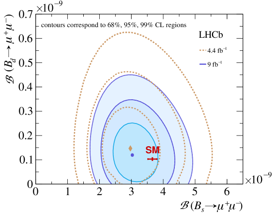
Figure 1: LHCb measurements of $\overline{\mathcal{B}}_{s\mu}$ and $\overline{\mathcal{B}}_{d\mu}$ at 4.4 and 9$\,{\rm fb}^{-1}$ integrated luminosity, compared to the current SM predictions. Plot from Fig. 2 of Ref. [7].

The SM description of $B_{s}\rightarrow\mu^{+}\mu^{-}$ is greatly simplified by a factorization of long- and short-distance Quantum Chromodynamics (QCD) effects. In contrast to many other $B$ decays, the SM decay amplitude of $B_{s}\rightarrow\mu^{+}\mu^{-}$ depends, to a very good approximation, only on a single non-perturbative hadronic quantity, namely the $B_{s}$-meson decay constant $f_{B_{s}}$. Its determinations from lattice simulations (see below) are mature and precise. Moreover, the hard QCD and electroweak (EW) corrections are, to a very good approximation, contained within a single Wilson coefficient $C_{A}$, which can be calculated in a standard, perturbative matching procedure as a series in the strong and electromagnetic couplings $\alpha_{s}$ and $\alpha_{e}$. Thanks to these properties, the SM calculations have reached a few percent accuracy. The current SM prediction for the branching ratio reads

$$\overline{\mathcal{B}}_{s\mu}^{SM}=(3.64\pm 0.12)\times 10^{-9}.$$ (2)

We describe its evaluation in the next sections. The numerical value in Eq. (2) has been obtained by updating the input parameters in the semi-numerical expressions of Ref. [10], and including the power-enhanced QED correction from Refs. [11, 12] that amounts to around $-0.5\%$. A difference with respect to $(3.66\pm 0.14)\times 10^{-9}$ in Ref. [12] is due to the parameter update. The above SM prediction is well in agreement with each individual measurement [5, 6, 7, 8], as well as with their average in Eq. (1).

In the SM, on top of the aforementioned FCNC loop suppression, $\overline{\mathcal{B}}_{s\mu}$ receives a helicity suppression by the mass-squared ratio $m_{\mu}^{2}/m^{2}_{B_{s}}$. One or both of these suppressions may be lifted in models with additional Higgs doublets or with a $Z^{\prime}$. In effect, one finds restrictions on allowed parameter spaces in, among others, Two Higgs Doublet Models (2HDMs) [13] and the Minimal Supersymmetric Standard Model [14]. In addition, several time-dependent observables in $B_{s}\rightarrow\mu^{+}\mu^{-}$ can be used to study potential BSM ${\rm CP}$-violation mechanisms [15].

The present review is organized as follows. In section 2, we present the effective Lagrangian and the branching ratio formula for $B_{s}\rightarrow\mu^{+}\mu^{-}$ in the SM. Sections 3 and 4 are devoted to describing, respectively, the perturbative QCD and EW corrections to the Wilson coefficient $C_{A}$. At the end of Section 4, the power-enhanced QED correction to $\overline{\mathcal{B}}_{s\mu}$ is discussed. In section 5, we summarize the current parameter update and evaluate the SM prediction for $\overline{\mathcal{B}}_{s\mu}$ (2) together with the corresponding uncertainty. We conclude in section 6. In Appendix A, we recall the derivation of the branching ratio formula. In Appendix B, we present the current SM prediction for $\overline{\mathcal{B}}_{d\mu}$, i.e. the average time-integrated branching ratio of $B^{0}\to\mu^{+}\mu^{-}$.

2 The effective Lagrangian and the branching ratio formula

The effective Lagrangian used to describe $B_{s}\rightarrow l^{+}l^{-},$ $l\in\{e,\mu,\tau\}$ in the SM is obtained through simultaneous integrating out of all fields heavier than the $b$ quark at the scale $\mu_{0}=\mathcal{O}(m_{t})$. It has the form

$$\mathcal{L}=\mathcal{L}_{\text{QCD}\times\text{QED}}(\text{fields lighter than }W)+\left[N\sum_{n}C_{n}Q_{n}+\mathrm{h.c.}\right],$$ (3)

where

$$N\equiv\frac{V_{tb}^{*}V_{ts}G_{F}^{2}M_{W}^{2}}{\pi^{2}},$$ (4)

$V_{ij}$ are the Cabibbo-Kobayashi-Maskawa (CKM) matrix elements, $G_{F}$ is the Fermi constant, while $M_{W}$ is the $W$-boson mass defined in the on-shell renormalization scheme. The local operators $Q_{n}$ are polynomials in the light fields and their derivatives. The Wilson coefficients $C_{n}$ can be treated as real-valued (up to negligible corrections) once the global normalization factor $N$ is set as in Eq. (4). The operators $Q_{n}$ are of mass-dimension 5 or higher, and have to be suppressed by powers of $1/M_{W}$ necessary to make the overall mass-dimension of $\mathcal{L}$ equal to 4. At the leading order in $1/M_{W}$ and $\alpha_{e}$, it is sufficient to consider the operators $Q_{n}$ where a $\Delta B=-\Delta S=-1$ flavour-changing quark current multiplies a lepton current. Moreover, the quark current must violate parity to annihilate the pseudoscalar $B_{s}$ meson. Once the Lorentz invariance is imposed, one is left with the following four operators only:

$$\begin{split}Q_{A}&\equiv[\bar{l}\gamma_{\alpha}\gamma_{5}l][\bar{b}\gamma^{\alpha}\gamma_{5}s]\equiv[\bar{l}\gamma_{\alpha}\gamma_{5}l]j^{\alpha}_{A}~{}~{},\\ Q_{V}&\equiv[\bar{l}\gamma_{\alpha}l]j^{\alpha}_{A}~{}~{},\\ Q_{P}&\equiv[\bar{l}\gamma_{5}l][\bar{b}\gamma_{5}s]\equiv[\bar{l}\gamma_{5}l]j_{P}~{}~{},\\ Q_{S}&\equiv[\bar{l}l]j_{P}~{}~{}.\end{split}$$ (5)

The Lagrangian (3) can be used to derive the formula for $\overline{\mathcal{B}}_{s\mu}$. A sketch of the derivation is given in Appendix A. While evaluating the contribution of $Q_{A}$ there, it becomes clear that $Q_{V}$ does not contribute at the leading order in $\alpha_{e}$. As far as $Q_{P}$ and $Q_{S}$ are concerned, their Wilson coefficients are computed in a matching to full SM amplitudes with the quark and lepton currents exchanging Higgs bosons. Such contributions are suppressed by $m_{b}^{2}/M_{W}^{2}$, and can be neglected as being of the same order as dimension-8 operator effects. Hence, neglecting these tiny effects, $\overline{\mathcal{B}}_{s\mu}$ in the SM depends on $C_{A}$ only. The explicit expression reads

$$\overline{\mathcal{B}}_{s\mu}^{SM}=\frac{|N|^{2}M_{B_{s}}^{3}f_{B_{s}}^{2}}{8\pi\Gamma_{H}^{s}}\beta r^{2}|C_{A}|^{2}+\mathcal{O}\left(\alpha_{e},\frac{m_{b}^{2}}{M_{W}^{2}}\right),$$ (6)

where $r\equiv 2m_{\mu}/M_{B_{s}}$, $\beta\equiv\sqrt{1-r^{2}}$, while $\Gamma_{H}^{s}$ is the heavier mass eigenstate width in the $B_{s}$–$\overline{B}_{s}$ system. Finally, the $B_{s}$ decay constant $f_{B_{s}}$ is defined through the relation

$$\braket{0}{j^{\alpha}_{A}(x)}{B_{s}(p)}\equiv ip^{\alpha}f_{B_{s}}e^{-ipx}.$$ (7)

It is calculated using lattice QCD methods with errors at a sub-percent level. The current world average based on $2+1+1$ simulations [16, 17, 18, 19] alone amounts to [20]

$$f_{B_{s}}=(230.3\pm 1.3)\,\text{MeV}.$$ (8)

In several popular BSMs, the Wilson coefficients $C_{S}$ and $C_{P}$ can become comparable in size to $rC_{A}$. For example, in the 2HDM-II with large $\tan\beta_{H}\equiv v_{2}/v_{1}$ (the ratio of the vacuum expectation values of the two Higgs doublets), one finds [21],

$$C_{S}\simeq C_{P}\simeq\frac{\ln\rho}{\rho-1}\frac{m_{\mu}m_{b}}{4M^{2}_{W}}\tan^{2}\beta_{H},$$ (9)

where $\rho\equiv M_{H^{+}}^{2}/m_{t}^{2}$. The SM suppression factor of $m_{b}^{2}/M_{W}^{2}$ can get compensated by values of $\tan\beta_{H}=\mathcal{O}(50)$ or larger. The branching ratio formula in the 2HDM becomes (see Appendix A)

$$\overline{\mathcal{B}}^{2HDM}_{s\mu}=\frac{|N|^{2}M_{B_{s}}^{3}f_{B_{s}}^{2}}{8\pi\Gamma_{H}^{s}}\beta\left[|rC_{A}-uC_{P}|^{2}+\frac{\Gamma_{H}^{s}}{\Gamma_{L}^{s}}|u\beta C_{S}|^{2}\right]+\mathcal{O}(\alpha_{e}),$$ (10)

where $u\equiv M_{B_{s}}/(m_{b}+m_{s})$ and $\Gamma_{L}^{s}$ is the lighter mass eigenstate width in the $B_{s}$–$\overline{B}_{s}$ system.

Coming back to the SM expression for $\overline{\mathcal{B}}_{s\mu}$ in Eq. (6), several comments concerning the $\mathcal{O}(\alpha_{e})$ terms there are necessary. First, all the corrections of this order to $C_{A}$ are already known and included in the numerical result in Eq. (2). They will be discussed in subsection 4.1. Some of them get enhanced by $1/\sin^{2}\theta_{W}$, $m_{t}^{2}/M_{W}^{2}$ or $\ln^{2}M_{W}^{2}/m_{b}^{2}$, where $\theta_{W}$ is the weak mixing angle. Second, some of the remaining electromagnetic corrections in the $\mathcal{O}(\alpha_{e})$ term in Eq. (6) receive a power enhancement by $M_{B_{s}}/\Lambda_{\text{QCD}}$ [11]. They come from virtual photons emitted by the $s$ quark, and absorbed by the leptons. We shall comment on them in subsection 4.2. Their evaluation requires extending the operator basis to include effects of other dimension-6 operators, not present in Eq. (5), such as

$$Q_{2}^{\dagger}\equiv[\bar{b}\gamma_{\alpha}P_{L}c][\bar{c}\gamma^{\alpha}P_{L}s]\hskip 28.45274pt\mbox{or}\hskip 28.45274ptQ_{7}^{\dagger}\equiv\frac{em_{b}}{16\pi^{2}}[\bar{b}\sigma^{\alpha\beta}P_{L}s]F_{\alpha\beta}~{}~{}.$$ (11)

Third, the dependence of $C_{A}$ on the renormalization scale $\mu_{b}$ (that arises due to QED effects only) induces around $\mathcal{O}(0.3\%)$ uncertainty in $\overline{\mathcal{B}}_{s\mu}^{SM}$ [10]. Such a dependence must be compensated by the yet unknown $\mathcal{O}(\alpha_{e})$ corrections that receive no extra enhancement factors.

3 The QCD corrections to $C_{A}$

As described in the previous section, at the leading order in $\alpha_{e}$ and $m_{b}^{2}/M_{W}^{2}$, the only significant short-distance parameter entering the SM branching ratio formula is the $C_{A}(\mu_{b})$ Wilson coefficient, where we specifically indicate its dependence on the low-energy renormalization scale $\mu_{b}=\mathcal{O}(m_{b})$. It is evaluated by demanding equality of corresponding Green’s functions in the SM and the effective theory (3) at the renormalization scale $\mu_{0}=\mathcal{O}(m_{t})$ at which the electroweak degrees of freedom are decoupled. Computationally, the simplest choice of a Green’s function for the extraction of $C_{A}$ is $G[\bar{b},s,\bar{l},l]$ with vanishing external momenta:

$$G_{SM}[\bar{b},s,\bar{l},l](\mu_{0})\rvert_{p_{i}=0}=G_{\rm eff}[\bar{b},s,\bar{l},l](\mu_{0})\rvert_{p_{i}=0}.$$ (12)

At the matching scale $\mu_{0}$, QCD on both sides is treated perturbatively. This equation is then solved for $C_{A}(\mu_{0})$ order-by-order in $\alpha_{s}$ and $\alpha_{e}$, resulting in a double series

$$C_{A}(\mu_{0})=\sum\limits_{m,n=0}^{\infty}\tilde{\alpha}_{s}^{m}\tilde{\alpha}_{e}^{n}C_{A}^{(m,n)}(\mu_{0}),$$ (13)

where $\alpha_{i}(\mu_{0})\equiv 4\pi\tilde{\alpha}_{i}$ are the running couplings renormalized in the $\overline{\text{MS}}$ scheme at the scale $\mu_{0}$. In this section, we focus on the leading terms in $\alpha_{e}$, namely $C_{A}^{(m,0)}$.

As we work at the leading order in $1/M_{W}$, all light masses in the matching equation (12) can be set to 0. In dimensional regularization, all scaleless loop integrals vanish. In consequence, on the effective theory side, one is left only with tree diagrams, including the UV-counterterm ones. On the SM side, partially massive tadpoles have to be calculated. Removing light masses from propagators in the SM Green’s function leads to spurious infrared divergences in loop integrals evaluated in $d=4-2\epsilon$ dimensions. The resulting additional $\epsilon$-poles are not removed by renormalization constants of the SM. Instead, they cancel in the matching equation (12) against the tree-level UV counterterms in the effective theory.

Once such a procedure is applied in our case, one has to supplement the effective Lagrangian with additional operators that vanish when $\epsilon\to 0$ due to the Dirac algebra identities. Such operators are called evanescent. The UV-counterterms with these operators cancel against some of the spurious infrared divergence effects on the SM side. Moreover, their Wilson coefficients evaluated at lower orders affect the physical operator Wilson coefficients at higher orders. For the $C_{A}^{(m,0)}$ terms, it is sufficient to introduce only one evanescent operator [22]:

$$Q_{A}^{E}=[\bar{b}\gamma_{\alpha}\gamma_{\beta}\gamma_{\delta}s][\bar{l}\gamma^{\delta}\gamma^{\beta}\gamma^{\alpha}l]-4Q_{A}.$$ (14)

The bare fields, couplings and Wilson coefficients on the effective side are replaced by the renormalized ones, with mixing occurring between the physical and evanescent operators:

$$C^{(b)}_{A}Q^{(b)}_{A}+C^{E(b)}_{A}Q^{E(b)}_{A}=Z_{q}Z_{l}(C_{A}Z_{NN}Q_{A}+C_{A}Z_{NE}Q_{A}^{E}+C_{A}^{E}Z_{EN}Q_{A}+C_{A}^{E}Z_{EE}Q_{A}^{E}),$$ (15)

where $Z_{q}$ and $Z_{l}$ are the quark- and lepton-field $\overline{\text{MS}}$ renormalization constants, respectively, with $Z_{l}=1+\mathcal{O}(\alpha_{e})$. To fix the renormalization constants $Z_{ij}$, one demands that in the renormalized Green’s functions, the terms proportional to $C_{A}$ are finite when $\epsilon\to 0$, while those proportional to $C_{A}^{E}$ vanish in this limit [23]. Examples of diagrams contributing to $Z_{ij}$ at $\alpha_{s}$ and $\alpha_{s}^{2}$ are shown in Fig. 2. Results for the relevant $Z_{ij}$ up to $\mathcal{O}(\alpha_{e}^{0}\alpha_{s}^{2})$ are given in Eq. (15) of Ref. [24].

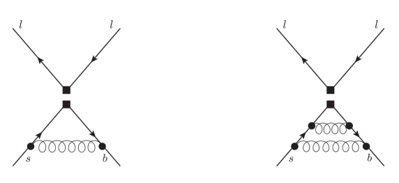
Figure 2: Examples of the Feynman diagrams appearing in the calculation of $Z_{ij}$. The double square in the middle denotes an insertion of either $Q_{A}$ or $Q_{A}^{E}$. Diagrams from Fig. 2 of Ref. [24].

It is important to emphasize that $Z_{NN}=1$ to all orders in QCD, once higher-dimensional operators and $\mathcal{O}(\alpha_{e})$ effects are neglected. Therefore, the Renormalization Group Equation (RGE) for $C_{A}$ is trivial at this level:

$$\mu\frac{d}{d\mu}C_{A}=\mathcal{O}(\alpha_{e}).$$ (16)

Consequently, there is no RG evolution of $C_{A}(\mu)$ at the leading order in $\alpha_{e}$:

$$C_{A}(\mu_{b})=C_{A}(\mu_{0})+\mathcal{O}(\alpha_{e}).$$ (17)

The SM Green’s function in Eq. (12) receives QCD corrections from two classes of diagrams: $W$-boxes and $Z$-penguins, shown in Fig. 3. Such bare diagrams get renormalized using lower-loop SM diagrams with counterterms. The QCD coupling constant renormalization $Z_{g}$ has to be modified by an appropriate threshold correction to match the coupling constant of the effective theory with only 5 active flavours (see section 3 in Ref. [25]). Similarly, the light-field wave-function renormalization constants have to be shifted to account for the decoupling threshold (see section 4 in Ref. [26]). Heavy fields and masses are renormalized in the $\overline{\text{MS}}$ scheme.

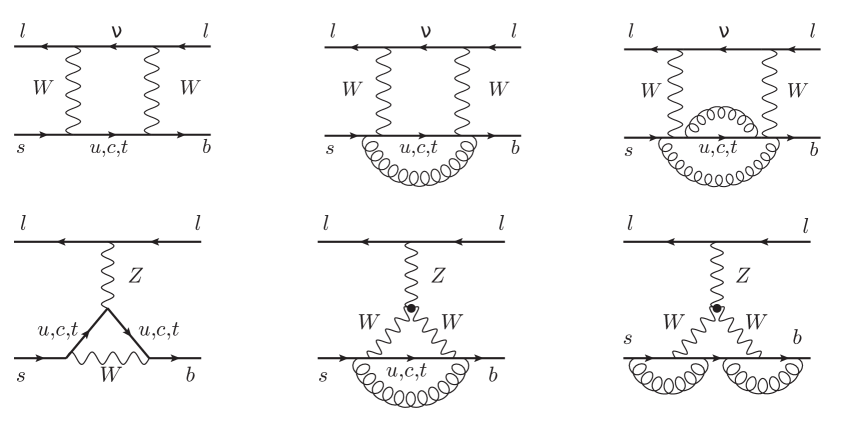
Figure 3: Examples of diagrams entering the SM side of the matching equation (12) at various orders in QCD. The $W$-boxes and $Z$-penguins are shown in the top and bottom rows, respectively. Contributions of the orders $\alpha_{s}^{0}$, $\alpha_{s}^{1}$, and $\alpha_{s}^{2}$ are arranged from left to right. Diagrams from Figs. 1 and 4 of Ref. [24].

Once both sides of the matching equation (12) have been properly renormalized, the value of $C_{A}(\mu_{0})$ can be extracted. All the Dirac structures appearing on the SM side are mapped onto either $Q_{A}$ or $Q_{A}^{E}$, and their coefficients compared to the ones on the effective side.

The procedure described in this section was completed in Ref. [27] at the leading order, followed by Refs. [28, 29, 22] and [24] for the $\mathcal{O}(\alpha_{s}^{1})$ and $\mathcal{O}(\alpha_{s}^{2})$ corrections, respectively. In the latter case, high-order expansions in $y\equiv M_{W}/m_{t}$ and $w\equiv 1-M_{W}^{2}/m_{t}^{2}$ were computed, and their combination was used to obtain a numerical result at the physical value of $M_{W}/m_{t}$.

4 The electroweak corrections

4.1 The $C_{A}^{(0,1)}$ correction

The next-to-leading order EW correction $C_{A}^{(0,1)}(\mu_{0})$ was first obtained in Ref. [30]. Its calculation follows a similar pattern to the one described in the previous section. The main difference comes from additional Dirac structures appearing in the $\mathcal{O}(\alpha_{e})$ corrections on the SM side of the matching equation, which necessitate including additional operators in the effective Lagrangian. For the complete matching at the scale $\mu_{0}$, at the leading order in $1/M_{W}$ and including $\mathcal{O}(\alpha_{e})$ terms, one has to retain all the operators from Eq. (5), and supplement them with $Q_{2}^{\dagger}$ defined in Eq. (11). The cancellation of spurious infrared divergence effects requires also the inclusion of additional evanescent operators (see Appendix A of Ref. [30]). The renormalization constants of all resulting Wilson coefficients are then calculated in a way analogous to the $C_{A}^{(m,0)}$ calculation.

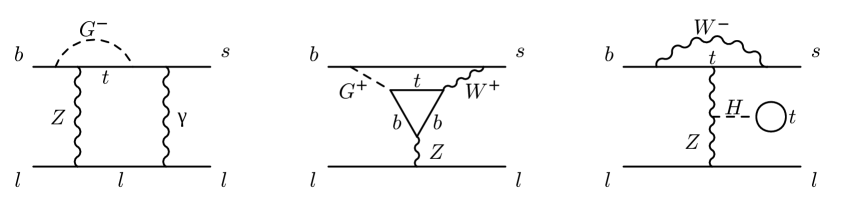
Figure 4: Examples of diagrams contributing to the $\mathcal{O}(\alpha_{e})$ EW correction on the SM side of the matching equation (12). Diagrams from Fig. 1 of Ref. [30].

Examples of diagrams contributing to $C_{A}^{(0,1)}(\mu_{0})$ on the SM side are shown in Fig. 4. Before this correction can be extracted, the UV divergences on the SM side have to be renormalized. For a discussion of different renormalization schemes for the electroweak boson and top quark masses, we refer to the original article [30]. Here, we will continue the analysis in the OS-2 scheme defined therein, as it was used in the subsequent phenomenological analysis [10]. In this scheme, all the QCD corrections to mass renormalization constants are defined in the $\overline{\text{MS}}$, but the $\mathcal{O}(\alpha_{e})$ corrections to $Z_{m_{t}}$, $Z_{M_{W}}$ and $Z_{M_{Z}}$ are defined on shell. In practice, the calculation was first done fully in the $\overline{\text{MS}}$ scheme, and the finite terms in these three renormalization constants were subsequently added to the renormalized results.

The value of $C_{A}$ extracted at the scale $\mu_{0}$ must then be RG-evolved down to the $\mu_{b}$ scale of the $B_{s}\to\mu^{+}\mu^{-}$ decay. The renormalized Wilson coefficients of the extended set of effective operators are related to the bare ones through a relation similar to Eq. (15):

$$C_{j}^{(b)}Q_{j}^{(b)}=Z_{q}Z_{l}\sum\limits_{k}C_{k}Z_{kj}Q_{j}\Longrightarrow C_{j}^{(b)}=\sum\limits_{k}C_{k}Z_{kj}.$$ (18)

The one-loop RGE for Wilson coefficients $\vec{C}$ has a general form

$$\mu\frac{d}{d\mu}\vec{C}=\left(\tilde{\alpha}_{s}\gamma_{s}^{(0)}+\tilde{\alpha}_{e}\gamma_{e}^{(0)}\right)^{T}\vec{C},$$ (19)

where the Anomalous Dimension Matrices (ADMs) $\gamma_{s}^{(0)}$ and $\gamma_{e}^{(0)}$ are obtained from the renormalization constants of Wilson coefficients. Once we restrict to non-evanescent operators only, the necessary MS-scheme relation reads

$$Z_{kj}=\delta_{kj}+\frac{1}{2\epsilon}\left[\tilde{\alpha}_{s}\gamma_{s}^{(0)}+\tilde{\alpha}_{e}\gamma_{e}^{(0)}\right]_{kj}+\mathcal{O}\left(\tilde{\alpha}_{s}^{2},\tilde{\alpha}_{e}^{2},\tilde{\alpha}_{s}\tilde{\alpha}_{e}\right).$$ (20)

For the RGE (19) to close, one has to extend the set of operators in the effective Lagrangian further (see the discussion under Eq. (15) in Ref. [30]). Analytical expressions for the evolution operator associated with Eq. (19) can be found, e.g., in Ref. [31]. The details and results of the numerical solution can be found in Appendix B of Ref. [30].

4.2 Power-enhanced QED corrections

Within the effective theory framework, the $S$-matrix element corresponding to the $B_{s}\to\mu^{+}\mu^{-}$ decay receives $\mathcal{O}(\alpha_{e})$ contributions from diagrams with tree-level Wilson coefficients and a virtual photon exchanged between the fermions. In particular, there is a class of diagrams with a photon emitted from the spectator $s$ quark and absorbed by one of the outgoing muons (see Fig. 5). The leading terms of the power series in $\{m_{s},m_{\mu},\Lambda_{\text{QCD}}\}/m_{b}$ of this correction were computed in Ref. [11]. It was observed that its helicity suppression by the factor of $r^{2}$ in the tree-level branching ratio (6) is partially lifted due to a relative enhancement by $M_{B_{s}}/\Lambda_{\text{QCD}}$.

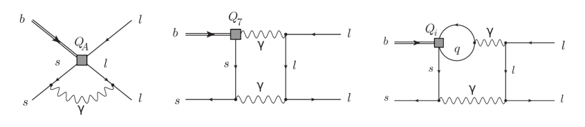
Figure 5: Examples of diagrams with virtual photon exchanges that are responsible for the power-enhanced QED correction in Eq. (23). Diagrams from Fig. 1 of Ref. [11].

Effects of hard virtual photons with energies and virtualities above the $\mu_{b}$ scale are contained in the Wilson coefficients $C_{i}$. The remaining virtual photons need to be taken into account in the physical matrix elements that are evaluated at the scale $\mu_{b}$. In particular, virtual photons exchanged in the diagrams in Fig. 5 probe the inner structure of the $B_{s}$ meson, smearing the annihilation point of the valence quarks over a distance $\mathcal{O}\left((M_{B_{s}}\Lambda_{\text{QCD}})^{-\frac{1}{2}}\right)$, which corresponds to inverse virtuality of the off-shell $s$ quark. Such long-distance QCD effects cannot be parameterized solely by $f_{B_{s}}$, as at the leading order. Instead, one has to estimate effects of matrix elements like

$$\braket{0}{\!\int\!d^{d}x\;\mathbf{T}[[\bar{\mu}\gamma^{\alpha}\mu](x)Q_{A}(0)]}{B_{s}},$$ (21)

where T is the time-ordering operator. They involve the $B$ meson light-cone distribution amplitude [32] and its first logarithmic moments.

Virtual photon exchanges leading to power-enhanced QED corrections were thoroughly studied in the formalism of the Soft-Collinear Effective Theory by Beneke, Bobeth and Szafron in Ref. [12]. Their effect can be included in the SM prediction through a replacement

$$\overline{\mathcal{B}}_{s\mu}\rightarrow\eta_{\scriptscriptstyle BBS}\overline{\mathcal{B}}_{s\mu}~{}~{},$$ (22)

with

$$\eta_{\scriptscriptstyle BBS}=0.995^{+0.003}_{-0.005}.$$ (23)

The main uncertainty in $\eta_{\scriptscriptstyle BBS}$ comes from poorly known values of hadronic parameters [33]. We have extracted the numerical value of $\eta_{\scriptscriptstyle BBS}$ as well as its uncertainty in Eq. (23) from Eqs. (8.8) and (8.10) of Ref. [12]. One can observe there that the relatively small central value of the correction ($-0.5\%$) arises as an effect of partial cancellation between potentially unrelated contributions from the $Q_{V}$ and $Q_{7}^{\dagger}$ operators. Thanks to this cancellation, the overall effect remains below the $\pm 1.5\%$ non-parametric uncertainty estimated in Ref. [10]. That uncertainty was primarily due to unknown $\mathcal{O}(\alpha_{e})$ effects, although the possibility of their power enhancement remained unknown at the time.

The contribution of $Q_{7}^{\dagger}$ to the considered corrections was reanalyzed in Ref. [34]. Despite several differences in the analytical expressions with respect to the earlier analysis of Ref. [12], the numerical results of the two papers remain in qualitative agreement, and no modification of the factor $\eta_{\scriptscriptstyle BBS}$ in Eq. (23) is necessary.

5 Numerical analysis

In this section, we update the SM prediction for $\overline{\mathcal{B}}_{s\mu}$ based on Eq. (6), including the complete $\mathcal{O}(\alpha_{s}^{2})$ and $\mathcal{O}(\alpha_{e})$ corrections to $C_{A}$, as well as the QED correction factor in Eq. (23). In practice, it is sufficient to use the semi-numerical expressions from Eq. (6) of Ref. [10], which gives

$$\overline{\mathcal{B}}_{s\mu}^{SM}\times 10^{9}=(3.65\pm 0.06)\left(\frac{M_{t}[{\rm GeV}]}{173.1}\right)^{\!\!3.06}\left(\frac{\alpha_{s}(M_{Z})}{0.1184}\right)^{\!\!\!-0.18}R_{s}\,\eta_{\scriptscriptstyle BBS}\,,$$ (24)

where

$$R_{s}=\left(\frac{f_{B_{s}}[{\rm MeV}]}{227.7}\right)^{\!2}\!\left(\frac{|V_{cb}|}{0.0424}\right)^{\!2}\!\left(\frac{|V_{tb}^{\star}V_{ts}/V_{cb}|}{0.980}\right)^{\!2}\frac{\tau_{H}^{s}\,[{\rm ps}]}{1.615}\,.$$ (25)

In the above expressions, all the explicitly displayed input parameters are normalized to their 2013 central values. In Table 1, we update these central values together with the corresponding uncertainties. All the remaining parameters are retained unaltered with respect to Table I of Ref. [10], as their update would not affect $\overline{\mathcal{B}}_{s\mu}$ in a noticeable manner – they are either very precisely measured or have little effect on $\overline{\mathcal{B}}_{s\mu}$.

Table 1: Numerical values of the updated input parameters.

Parameter		Value		Unit		Ref.
$f_{B_{s}}$		230.3 (1.3)		MeV		[20, 16, 17, 18, 19]
$|V_{cb}|\times 10^{3}$		41.97 (48)		-		[35]
$|V_{tb}^{*}V_{ts}/V_{cb}|$		0.9820 (4)		-		derived from Ref. [36]
$\tau_{H}^{s}$		1.622 (8)		ps		[37]
$M_{t}$		172.57 (29)		GeV		[9]
$\alpha_{s}(M_{Z})$		0.1180 (9)		-		[9]

As already mentioned in Eq. (2), we find $\overline{\mathcal{B}}_{s\mu}^{SM}=(3.64\pm 0.12)\times 10^{-9}$. The overall uncertainty is now almost a factor of two smaller than found in Ref. [10], while the central value remains almost unchanged. The latter fact can be attributed to an approximate cancellation of shifts stemming from the parameter updates and $\eta_{\scriptscriptstyle BBS}$, as in the following sum:

$$+2.3\%(f_{B_{s}})-1.6\%(CKM)+0.4\%(\tau_{H}^{s})-0.9\%(M_{t})+0.1\%(\alpha_{s})-0.5\%(\eta_{\scriptscriptstyle BBS})\simeq-0.3\%.$$ (26)

As far as the uncertainty breakdown is concerned, its current version is compared to the 2013 one [10] in Table 2. In its last column, the uncertainties are combined in quadrature.

Table 2: The current uncertainty breakdown in $\overline{\mathcal{B}}_{s\mu}^{SM}$, as compared to the 2013 one.

	$f_{B_{s}}$	CKM	$\tau_{H}^{s}$	$M_{t}$	$\alpha_{s}$	$\eta_{\scriptscriptstyle BBS}$	other	non-	$\sum$
								parametric
2024 [this paper]	$1.1$%	$2.3\%$	$0.5$%	$0.5$%	$0.1$%	$0.5$%	$<0.1$%	$1.5$%	$3.2$%
2013 [10]	$4.0$%	$4.3\%$	$1.3$%	$1.6$%	$0.1$%	$0.0$%	$<0.1$%	$1.5$%	$6.4$%

One can observe a significant improvement in the first four columns where the dominant parametric uncertainties originate from, in particular in the case of $f_{B_{s}}$ that is determined on the lattice. As far as the top-quark mass $M_{t}$ is concerned, let us recall that the PDG [9] value is treated as the on-shell mass, which is not strictly correct. However, the overall non-parametric uncertainty of $\pm 1.5\%$ is understood to contain a contribution from such an approximation. As it is evident from Tables 1 and 2, a $300\;{\rm MeV}$ shift in $M_{t}$ implies a $0.5\%$ shift in $\overline{\mathcal{B}}_{s\mu}^{SM}$.

At present, the most important uncertainty originates from $|V_{cb}|$, in which case we use the inclusive determination only [35]. A combination with exclusive determinations would not lead to an improvement, given the persistent discrepancy between the inclusive and exclusive results [9]. Our preference is the same as in Ref. [10], i.e. we treat the inclusive determination as theoretically cleaner, and more reliable.

As already mentioned in Ref. [10], one can get rid of $|V_{cb}|$ in the ratio of $\overline{\mathcal{B}}_{s\mu}$ to the measured $B_{s}^{(H)}$-$B_{s}^{(L)}$ mass difference, at the cost of introducing an extra uncertainty from lattice determinations of the “bag parameter” $B_{B_{s}}$. Such an approach is likely to become relevant once the experimental accuracy in $\overline{\mathcal{B}}_{s\mu}$ (currently $8.1\%$ in Eq. (1)) becomes closer to the theoretical one.

6 Conclusions

In this review, we analyzed the current SM prediction for the branching ratio of the rare $B_{s}\to\mu^{+}\mu^{-}$ decay. This channel continues to be among the most promising candidates for detecting BSM physics without direct production of new particles, due to its SM suppression and possible BSM enhancements.

The SM analysis is, to a very good approximation, contained in the perturbative calculation of the Wilson coefficient $C_{A}$, and the lattice calculation of the long-distance QCD parameter $f_{B_{s}}$. The perturbative part was already complete up to and including next-to-next-to-leading QCD and next-to-leading EW effects.

The currently dominant theoretical uncertainty originates from the CKM-matrix element $|V_{cb}|$. The next-to-dominant uncertainty is already non-parametric, stemming mainly from the unknown higher-order electromagnetic corrections at the scale $\mu_{b}$. They depend on non-perturbative effects that are not contained in $f_{Bs}$. The current result for $\overline{\mathcal{B}}_{s\mu}^{SM}$ changes by around $0.3\%$ when $\mu_{b}$ is varied between $m_{b}/2$ and $2m_{b}$. However, since it provides a lower bound only on the possible size of unknown electromagnetic effects, the actual uncertainty estimate should be somewhat more conservative. Here, we have retained the overall non-parametric uncertainty at the same level as in Ref. [10], namely $\pm 1.5\%$.

The experimental error is currently much larger, around 8%, which sets a limit on the power of $B_{s}\to\mu^{+}\mu^{-}$ as a means for testing various BSM theories. The situation is expected to improve with time, when higher statistics get collected at the LHC and future experiments.

A final message that we would like to share with the reader is as follows. Our numerical result in Eq. (2) will become outdated as soon as any of the input parameters gets determined in a new analysis. Performing another update of $\overline{\mathcal{B}}_{s\mu}^{SM}$ does not require being an expert. It is sufficient to substitute new inputs into the simple formula (24).

Acknowledgements: This work was supported by the National Science Center, Poland, under the research project 2020/37/B/ST2/02746.

Appendix A The branching ratio formula

In this appendix, we sketch the derivation of the branching ratio formula (10) that holds in models with SM-like ${\rm CP}$-violation, including the SM and the 2HDM. We work at the leading order in QED throughout, i.e. the final-state muons are understood to be emitted directly from the operator vertex ($Q_{A}$, $Q_{P}$ or $Q_{S}$).

Let $\ket{B_{s}}$ and $\ket{\overline{B}_{s}}$ denote the meson flavour eigenstates with valence quarks $\bar{b}s$ and $b\bar{s}$, respectively. We fix conventions in their overall phases by demanding that  ${\rm CP}\ket{B_{s}}=\ket{\overline{B}_{s}}$,  and ${\rm CPT}\ket{B_{s}}=\ket{\overline{B}_{s}}$. Once this is done, the heavier ($H$) and lighter ($L$) mass eigenstates (see section 13 of Ref. [9]) can respectively be written as

$$\ket{B_{s}^{(H)}}=\frac{1}{\sqrt{2}|N|}\left(N^{*}\ket{B_{s}}-N\ket{\overline{B}_{s}}\right),\hskip 28.45274pt\ket{B_{s}^{(L)}}=\frac{1}{\sqrt{2}|N|}\left(N^{*}\ket{B_{s}}+N\ket{\overline{B}_{s}}\right),$$ (A1)

where $N$ has been defined in Eq. (4). In the limit of no ${\rm CP}$-violation ($N=|N|$), $B_{s}^{(H)}$ and $B_{s}^{(L)}$ are ${\rm CP}$-odd and ${\rm CP}$-even, respectively.

From the form of the lepton currents in Eq. (5), we observe that the $Q_{A}$ and $Q_{P}$ interactions can lead to production of ${\rm CP}$-odd lepton pairs only (in the CM frame), while $Q_{S}$ can lead to production of ${\rm CP}$-even pairs only. In the $Q_{A}$ case, it follows from the fact that the timelike component of the lepton current is ${\rm CP}$-odd (see, e.g., the table below Eq. (3.150) of Ref. [38]), while the spacelike components play no role, as they get contracted with vanishing spacelike components of the meson momentum (see Eq. (7)).

Let us now show that even in the presence of SM-like ${\rm CP}$-violation, ($N\neq|N|$ but real Wilson coefficients), the operators $Q_{A}$ and $Q_{P}$ have no effect on dimuonic decays of $B_{s}^{(L)}$, while $Q_{S}$ has no effect on such decays of $B_{s}^{(H)}$. When the “${\mathrm{h}.c.}$” terms in the Lagrangian (3) are taken into account, the leading $Q_{A}$ contribution to the $B_{s}^{(L)}$ decay amplitude is proportional to

$$\bra{\mu^{+}\mu^{-}}NQ_{A}+N^{*}Q_{A}^{\dagger}\ket{B_{s}^{(L)}}=\frac{|N|}{\sqrt{2}}\left(\bra{\mu^{+}\mu^{-}}Q_{A}\ket{B_{s}}+\bra{\mu^{+}\mu^{-}}Q_{A}^{\dagger}\ket{\overline{B}_{s}}\right),$$ (A2)

where the matrix elements on the r.h.s. are the only two that do not vanish due to flavour conservation in QCD. Next, we observe that

$$\bra{\mu^{+}\mu^{-}}Q_{A}^{\dagger}\ket{\overline{B}_{s}}=\bra{\mu^{+}\mu^{-}}({\rm CP})^{\dagger}Q_{A}{\rm CP}\ket{\overline{B}_{s}}=-\bra{\mu^{+}\mu^{-}}Q_{A}\ket{B_{s}},$$ (A3)

where we have taken advantage of the fact that the dimuon state is ${\rm CP}$-odd, as argued above. Consequently, the sum of the two matrix elements on the r.h.s. of Eq. (A2) vanishes. An identical reasoning holds for $Q_{P}$. As far as $Q_{S}$ and $B_{s}^{(H)}$ are concerned, we proceed by analogy:

$$\bra{\mu^{+}\mu^{-}}NQ_{S}+N^{*}Q_{S}^{\dagger}\ket{B_{s}^{(H)}}=\frac{|N|}{\sqrt{2}}\left(\bra{\mu^{+}\mu^{-}}Q_{S}\ket{B_{s}}-\bra{\mu^{+}\mu^{-}}Q_{S}^{\dagger}\ket{\overline{B}_{s}}\right),$$ (A4)

$$\bra{\mu^{+}\mu^{-}}Q_{S}^{\dagger}\ket{\overline{B}_{s}}=\bra{\mu^{+}\mu^{-}}({\rm CP})^{\dagger}Q_{S}{\rm CP}\ket{\overline{B}_{s}}=\bra{\mu^{+}\mu^{-}}Q_{S}\ket{B_{s}},$$ (A5)

where this time the dimuon state is ${\rm CP}$-even. Consequently, the difference of the two matrix elements on the r.h.s. of Eq. (A4) vanishes. As a by-product of the above reasoning, we can simplify the non-vanishing matrix elements as follows:

$$\begin{split}\bra{\mu^{+}\mu^{-}}NQ_{A,P}+N^{*}Q_{A,P}^{\dagger}\ket{B_{s}^{(H)}}&=|N|\sqrt{2}\bra{\mu^{+}\mu^{-}}Q_{A,P}\ket{B_{s}},\\ \bra{\mu^{+}\mu^{-}}NQ_{S}+N^{*}Q_{S}^{\dagger}\ket{B_{s}^{(L)}}&=|N|\sqrt{2}\bra{\mu^{+}\mu^{-}}Q_{S}\ket{B_{s}}.\end{split}$$ (A6)

Both at the LHC and at $e^{+}e^{-}$ machines, the production rates of $B_{s}$ and $\overline{B}_{s}$ are practically equal. Thus, to a very good approximation, the heavy and light mass eigenstates are produced in the same quantities, as can be seen by inverting the relation (A1). Since the decay products of $B_{s}^{(H)}$ (${\rm CP}$-odd dimuons) and $B_{s}^{(L)}$ (${\rm CP}$-even dimuons) do not interfere, the average time-integrated branching ratio is simply given by

$$\overline{\mathcal{B}}_{s\mu}=\frac{1}{2}\left(\frac{\Gamma[B^{(H)}_{s}\rightarrow\mu^{+}\mu^{-}]}{\Gamma_{H}^{s}}+\frac{\Gamma[B^{(L)}_{s}\rightarrow\mu^{+}\mu^{-}]}{\Gamma_{L}^{s}}\right).$$ (A7)

In each of the two cases, the decay rate is given by the well-known formula

$$\Gamma[B^{(H,L)}_{s}\rightarrow\mu^{+}\mu^{-}]=\frac{1}{2M_{B_{s}}}\int dPS_{2}\left|\overline{{\mathcal{M}}}^{(H,L)}\right|^{2}=\frac{\beta}{16\pi M_{B_{s}}}\left|\overline{{\mathcal{M}}}^{(H,L)}\right|^{2},$$ (A8)

with

$$dPS_{2}=\frac{1}{4\pi^{2}}\,d^{4}k_{+}\,d^{4}k_{-}\,\delta(k_{+}^{2}-m_{\mu}^{2})\theta(k^{0}_{+})\,\delta(k_{-}^{2}-m_{\mu}^{2})\theta(k^{0}_{-})\,\delta^{(4)}(p-k_{+}-k_{-}).$$ (A9)

Here, ${\mathcal{M}}^{(H,L)}$ are the corresponding invariant matrix elements, $\beta$ has been defined below Eq. (6), and we have neglected the tiny mass splitting between $B_{s}^{(H)}$ and $B_{s}^{(L)}$. Summing over spins of the final-state muons is understood in Eq. (A8). The two-body phase-space integral is trivial, as $\left|\overline{{\mathcal{M}}}^{(H,L)}\right|^{2}$ is constant in the integration domain due to rotational symmetry in the decaying scalar rest frame.

The $Q_{A}$ (and $Q_{A}^{\dagger}$) contribution to ${\mathcal{M}}^{(H)}$ reads

$${\mathcal{M}}^{(H)}_{A} = iC_{A}|N|\sqrt{2}\,e^{ipx}\bra{0}j^{\alpha}_{A}(x)\ket{B_{s}(p)}\,\bar{u}(k_{-})\gamma^{\alpha}\gamma_{5}\,v(k_{+})$$ (A10)

$$= -f_{B_{s}}C_{A}|N|\sqrt{2}\,\bar{u}(k_{-})\not{p}\gamma_{5}\,v(k_{+}),$$

where the identity (A6) has already been taken into account. Moreover, the $\ket{B_{s}}$ state normalization has been adjusted to the one that is conventionally used in the decay-constant definition (7), namely

$$\braket{B_{s}(q)}{B_{s}(p)}=2p_{0}(2\pi)^{3}\delta^{(3)}\left(\vec{p}-\vec{q}\right).$$ (A11)

To verify that the global normalization in Eq. (A10) is correct, one can begin with the relevant $S$ matrix element

$$\braket{S}\equiv{}_{\rm out}\!\braket{\mu^{+}\mu^{-}}{B_{s}^{(H,L)}}_{\rm in}=\braket{l^{+}l^{-}}{\mathbf{T}[\exp(i\int d^{4}x\,\mathcal{L}_{\rm int})]}{B_{s}^{(H,L)}}.$$ (A12)

In its evaluation, the $B_{s}$ meson hadronic structure cannot be treated in a perturbative manner. Therefore, in the definition of the in/out states in the above equation, the interaction part of the Lagrangian $\mathcal{L}_{\rm int}$ that is switched off at timelike infinities, consists only of the weak part $N\sum_{n}C_{n}Q_{n}+{\mathrm{h}.c.}$. It is assumed that non-perturbative QCD effects have been solved beforehand, and are contained in $\ket{B_{s}^{(H,L)}}_{\rm in}$ that is treated as an asymptotic state from the weak interaction perspective.

In practice, the right normalization in Eq. (A10) can be determined with possibly least effort by considering an analogy with a certain purely perturbative theory. Suppose the muons interact with a massive real pseudoscalar $\phi$ via a dimension-five operator $\widetilde{{\mathcal{L}}}_{\rm int}=\frac{\lambda}{M}(\partial^{\alpha}\phi)\bar{\mu}\gamma_{\alpha}\gamma_{5}\mu$. Once the tree-level invariant matrix element ${\mathcal{M}}$ for the decay $\phi\to\mu^{+}\mu^{-}$ is quickly determined, it should be expressed in terms of the free-field matrix element  $e^{ipx}\bra{0}\frac{\lambda}{M}\partial^{\alpha}\phi(x)\ket{\phi(p)}$, with the free-particle state $\ket{\phi(p)}$ normalized as in Eq. (A11). Finally, replacing

$$e^{ipx}\bra{0}\frac{\lambda}{M}\partial^{\alpha}\phi(x)\ket{\phi(p)}\hskip 28.45274pt\mbox{by}\hskip 28.45274ptC_{A}|N|\sqrt{2}\,e^{ipx}\bra{0}j^{\alpha}_{A}(x)\ket{B_{s}(p)},$$

(see Eq. (A6)), one obtains Eq. (A10) with the proper overall normalization.

The r.h.s. of Eq. (A10) can be further simplified by noticing that

$$\bar{u}\not{p}\gamma_{5}\,v=\bar{u}(\not{k}_{-}+\not{k}_{+})\gamma_{5}\,v=\bar{u}(\not{k}_{-}\gamma_{5}-\gamma_{5}\not{k}_{+})v=2m_{\mu}\bar{u}\gamma_{5}v,$$ (A13)

where the identities $\bar{u}(k_{-})\not{k}_{-}=m_{\mu}\bar{u}(k_{-})$,  and  $\not{k}_{+}v(k_{+})=-m_{\mu}v(k_{+})$  have been used in the last step. Let us note that our expression would vanish in the absence of $\gamma_{5}$, which is related to the vanishing divergence of the vectorlike current, the same one that enters the QED interactions of muons and photons. This is precisely the reason why we were allowed to skip $Q_{V}$ in our initial operator list in Eq. (5).

Let us now turn to the operators $Q_{P}$ and $Q_{S}$. The pseudoscalar current $j_{P}=\bar{b}\gamma_{5}s$ that is present in both of them can be eliminated in favour of the axial current $j_{A}^{\mu}$ using Equations of Motion (EoM) for the $s$- and $\bar{b}$-quark operator fields:

$$\begin{split}[i\not{\partial}-g\not{A}^{a}T^{a}-e\not{A}-m_{s}]s&\underset{\text{EoM}}{=}\mathcal{O}(M_{W}^{-2}),\\ \bar{b}[i\overset{\leftarrow}{\not{\partial}}+g\not{A}^{a}T^{a}+e\not{A}+m_{b}]&\underset{\text{EoM}}{=}\mathcal{O}(M_{W}^{-2}),\end{split}$$ (A14)

where $g$ and $e$ are the QCD and QED couplings respectively, $A_{\mu}^{a}$ is the gluon field, $A_{\mu}$ is the photon field, and $T^{a}$ are the SU(3) generators. The $\mathcal{O}(M_{W}^{-2})$ effects on the r.h.s. of the above equations stand for higher-order weak-interaction effects that stem from the operators $Q_{n}$ in Eq. (3). Such effects will be neglected below, as we are going to use the EoM to transform the weak operators $Q_{P}$ and $Q_{S}$, while we work at the leading order in weak interactions. Operators that vanish by the EoM will commonly be denoted by $\boxed{E}$. They can be skipped in evaluation of observables at the leading order in weak interactions, as their physical matrix elements vanish.

To proceed, we multiply the first equation in (A14) by $(\bar{b}\gamma_{5})$ from the left, the second one by $(\gamma_{5}s)$ from the right, take their difference, rearrange, and obtain

$$\partial_{\alpha}j_{A}^{\alpha}=i(m_{b}+m_{s})j_{P}+\boxed{E}.$$ (A15)

Using the above identity, one can express the following total derivative as

$$\partial_{\alpha}[(\bar{l}l)j_{A}^{\alpha}]=j_{A}^{\alpha}\partial_{\alpha}[\bar{l}l]+i(m_{b}+m_{s})Q_{S}+\boxed{E}.$$ (A16)

Consequently,

$$Q_{S}=\frac{(i\partial_{\alpha}[\bar{l}l])j_{A}^{\alpha}}{m_{b}+m_{s}}+\boxed{E}+\boxed{T},$$ (A17)

where $\boxed{T}$ commonly denotes total derivatives of operators that are invariant under QCD and QED gauge transformations. Similarly,

$$Q_{P}=\frac{(i\partial_{\alpha}[\bar{l}\gamma_{5}l])j_{A}^{\alpha}}{m_{b}+m_{s}}+\boxed{E}+\boxed{T}.$$ (A18)

Since $\boxed{T}$ in the Lagrangian has no effect on physical observables, we are allowed to replace $Q_{S}$ and $Q_{P}$ by the first (explicit) terms in the above equations. After such replacements, the same quark current shows up in $Q_{A}$, $Q_{S}$ and $Q_{P}$, which means that only a single non-perturbative quantity, namely $f_{B_{s}}$, is sufficient to describe their physical matrix elements at the leading order in QED.

Using Eqs. (A17)–(A18), and performing calculations along the same way as in the case of $Q_{A}$, one obtains

$$\mathcal{M}_{P}^{(H)}=\frac{M^{2}_{B_{s}}f_{B_{s}}}{m_{b}+m_{s}}C_{P}|N|\sqrt{2}\,\bar{u}(k_{-})\gamma_{5}\,v(k_{+}),$$ (A19)

and

$$\mathcal{M}_{S}^{(L)}=\frac{M^{2}_{B_{s}}f_{B_{s}}}{m_{b}+m_{s}}C_{S}|N|\sqrt{2}\,\bar{u}(k_{-})v(k_{+}).$$ (A20)

The total invariant matrix element for $B_{s}^{(H)}$ reads

$$\mathcal{M}^{(H)}=\mathcal{M}_{P}^{(H)}+\mathcal{M}_{A}^{(H)}=\left(\frac{M_{B_{s}}C_{P}}{m_{b}+m_{s}}-\frac{2m_{\mu}C_{A}}{M_{B_{s}}}\right)M_{B_{s}}f_{B_{s}}|N|\sqrt{2}\,\bar{u}(k_{-})\gamma_{5}\,v(k_{+}).$$ (A21)

It remains to take the moduli squared and perform the sums over spins:

$$\begin{split}\sum_{\rm spins}|\bar{u}\gamma_{5}\,v|^{2}&=-{\rm Tr}\left[(\not{k}_{-}+m_{\mu})\gamma_{5}(\not{k}_{+}-m_{\mu})\gamma_{5}\right]=2M_{B_{s}}^{2},\\ \sum_{\rm spins}|\bar{u}v|^{2}&={\rm Tr}\left[(\not{k}_{-}+m_{\mu})(\not{k}_{+}-m_{\mu})\right]=2M_{B_{s}}^{2}\beta^{2}.\end{split}$$ (A22)

Finally, after substitution to Eq. (A8), and then (A7), we end up with the branching ratio formula quoted in Eq. (10).

In BSM models with generic (not SM-like) ${\rm CP}$-violation, the Wilson coefficients $C_{A}$, $C_{P}$ and $C_{S}$ are not necessarily real. Moreover, the mass eigenstates are not necessarily given by Eq. (A1), as the phase factors may differ from $N/|N|$ and $N^{*}/|N|$. The latter effect can be described by introducing an extra complex phase $\phi_{s}^{BSM}\simeq\phi_{s}^{c\bar{c}s}-\arg[(V^{*}_{ts}V_{tb})^{2}]$, see section 2.2 of Ref. [15]. In such models, the branching ratio formula generalizes to

$$\overline{\mathcal{B}}_{s\mu}=\frac{|N|^{2}M_{B_{s}}^{3}f_{B_{s}}^{2}}{8\pi\Gamma_{H}^{s}}\beta\left[|rC_{A}-uC_{P}|^{2}F_{P}+|u\beta C_{S}|^{2}F_{S}\right]+\mathcal{O}(\alpha_{e}),$$ (A23)

with

$$\begin{split}F_{P}&\equiv 1-\frac{\Gamma_{L}^{s}-\Gamma_{H}^{s}}{\Gamma_{L}^{s}}\sin^{2}\left[\frac{1}{2}\phi_{s}^{\rm BSM}+\arg(rC_{A}-uC_{P})\right],\\ F_{S}&\equiv 1-\frac{\Gamma_{L}^{s}-\Gamma_{H}^{s}}{\Gamma_{L}^{s}}\cos^{2}\left[\frac{1}{2}\phi_{s}^{\rm BSM}+\arg(rC_{S})\right].\end{split}$$ (A24)

The above expressions for $F_{P}$ and $F_{S}$ have been derived from the results of Refs. [40, 41] where an interesting discussion concerning time-dependent observables can be found.

Appendix B Numerical update for $\overline{\mathcal{B}}_{d\mu}^{SM}$

Table B1: Numerical values of the extra input parameters that matter for $\overline{\mathcal{B}}_{d\mu}$.

Parameter		Value		Unit		Ref.
$f_{B_{d}}$		190.0 (1.3)		MeV		[20, 16, 17, 18, 19]
$|V_{tb}^{*}V_{td}|$		0.00851 (10)		-		derived from Ref. [36]
$\tau_{\rm av}^{d}$		1.517 (4)		ps		[37]

Here, we present the current SM prediction for $\overline{\mathcal{B}}_{d\mu}$, i.e. the average time-integrated branching ratio of $B^{0}\to\mu^{+}\mu^{-}$. The necessary formula is analogous to Eq. (24), obtained by combining the semi-numerical expression from Eq. (7) of Ref. [10] with $\eta_{\scriptscriptstyle BBS}$ (23) derived from Ref. [12]. It reads

$$\overline{\mathcal{B}}^{\rm SM}_{d\mu}\times 10^{10}=(1.06\pm 0.02)\left(\frac{M_{t}[{\rm GeV}]}{173.1}\right)^{\!\!3.06}\left(\frac{\alpha_{s}(M_{Z})}{0.1184}\right)^{\!\!\!-0.18}R_{d}\,\eta_{\scriptscriptstyle BBS}\,,$$ (B1)

where

$$R_{d}=\left(\frac{f_{B_{d}}[{\rm MeV}]}{190.5}\right)^{\!2}\!\left(\frac{|V_{tb}^{\star}V_{td}|}{0.0088}\right)^{\!2}\frac{\tau_{\rm av}^{d}\,[{\rm ps}]}{1.519}\,.$$ (B2)

As input, we need three more parameters in addition to those already listed in Table 1, namely the decay constant $f_{B_{d}}$ of the $B^{0}$ meson, the average lifetime of this meson $\tau_{\rm av}^{d}$, and the relevant CKM factor $|V_{tb}^{*}V_{td}|$. Their current values are listed in Table B1. Our use of the well-measured $\tau_{\rm av}^{d}$ instead of $\tau_{H}^{d}$ is a good approximation thanks to the very small width difference predicted in the SM for the $B^{0}$-${\overline{B}}^{0}$ system: $\Delta\Gamma_{d}/(2\Gamma^{d}_{\rm av})=0.00172(46)$ [42].

After substituting all the numerical inputs to Eq. (B1), we find

$$\overline{\mathcal{B}}^{\rm SM}_{d\mu}=(9.71\pm 0.33)\times 10^{-11}.$$ (B3)

The uncertainty breakdown is presented in Table B2, in the same manner as it was done for $\overline{\mathcal{B}}^{\rm SM}_{s\mu}$ in Table 2.

Table B2: The current uncertainty breakdown in $\overline{\mathcal{B}}_{d\mu}^{SM}$, as compared to the 2013 one.

	$f_{B_{d}}$	CKM	$\tau_{\rm av}^{d}$	$M_{t}$	$\alpha_{s}$	$\eta_{\scriptscriptstyle BBS}$	other	non-	$\sum$
								parametric
2024 [this paper]	$1.4$%	$2.4\%$	$0.3$%	$0.5$%	$0.1$%	$0.5$%	$<0.1$%	$1.5$%	$3.4$%
2013 [10]	$4.5$%	$6.9\%$	$0.5$%	$1.6$%	$0.1$%	$0.0$%	$<0.1$%	$1.5$%	$8.5$%

References

- [1] G. Aad et al. [ATLAS], “Observation of a new particle in the search for the Standard Model Higgs boson with the ATLAS detector at the LHC,” Phys. Lett. B 716 (2012) 1 [arXiv:1207.7214].
- [2] S. Chatrchyan et al. [CMS], “Observation of a New Boson at a Mass of 125 GeV with the CMS Experiment at the LHC,” Phys. Lett. B 716 (2012) 30 [arXiv:1207.7235].
- [3] W. Altmannshofer and P. Stangl, “New physics in rare decays after Moriond 2021,” Eur. Phys. J. C 81 (2021) 952 [arXiv:2103.13370].
- [4] R. Aaij et al. [LHCb], “First Evidence for the Decay ,” Phys. Rev. Lett. 110 (2013) 021801 [arXiv:1211.2674].
- [5] A. M. Sirunyan et al. [CMS], “Measurement of properties of decays and search for with the CMS experiment,” JHEP 04 (2020) 188 [arXiv:1910.12127].
- [6] A. Tumasyan et al. [CMS], “Measurement of the decay properties and search for the decay in proton-proton collisions at = 13 TeV,” Phys. Lett. B 842 (2023) 137955 [arXiv:2212.10311].
- [7] R. Aaij et al. [LHCb], “Analysis of Neutral -Meson Decays into Two Muons,” Phys. Rev. Lett. 128 (2022) 041801 [arXiv:2108.09284].
- [8] M. Aaboud et al. [ATLAS], “Study of the rare decays of and mesons into muon pairs using data collected during 2015 and 2016 with the ATLAS detector,” JHEP 04 (2019), 098 [arXiv:1812.03017].
- [9] S. Navas et al. [Particle Data Group] “Review of Particle Physics,” Phys. Rev. D 110 (2024) 030001 (to be published, available at https://pdg.lbl.gov).
- [10] C. Bobeth, M. Gorbahn, T. Hermann, M. Misiak, E. Stamou and M. Steinhauser, “ in the Standard Model with Reduced Theoretical Uncertainty,” Phys. Rev. Lett. 112 (2014) 101801 [arXiv:1311.0903].
- [11] M. Beneke, C. Bobeth and R. Szafron, “Enhanced electromagnetic correction to the rare -meson decay ,” Phys. Rev. Lett. 120 (2018) 011801 [arXiv:1708.09152].
- [12] M. Beneke, C. Bobeth and R. Szafron, “Power-enhanced leading-logarithmic QED corrections to ,” JHEP 10 (2019) 232 [erratum: JHEP 11 (2022) 099] [arXiv:1908.07011].
- [13] A. Arbey, F. Mahmoudi, O. Stal and T. Stefaniak, “Status of the Charged Higgs Boson in Two Higgs Doublet Models,” Eur. Phys. J. C 78 (2018) 182 [arXiv:1706.07414].
- [14] A. Arbey, M. Battaglia and F. Mahmoudi, “Constraints on the MSSM from the Higgs Sector: A pMSSM Study of Higgs Searches, and Dark Matter Direct Detection,” Eur. Phys. J. C 72 (2012) 1906 [arXiv:1112.3032].
- [15] A. J. Buras, R. Fleischer, J. Girrbach and R. Knegjens, “Probing New Physics with the Time-Dependent Rate,” JHEP 07 (2013) 077 [arXiv:1303.3820].
- [16] A. Bazavov, C. Bernard, N. Brown, C. Detar, A. X. El-Khadra, E. Gámiz, S. Gottlieb, U. M. Heller, J. Komijani and A. S. Kronfeld, et al. “- and -meson leptonic decay constants from four-flavor lattice QCD,” Phys. Rev. D 98 (2018) 074512 [arXiv:1712.09262].
- [17] A. Bussone et al. [ETM], “Mass of the quark and -meson decay constants from twisted-mass lattice QCD,” Phys. Rev. D 93 (2016) 114505 [arXiv:1603.04306].
- [18] R. J. Dowdall et al. [HPQCD], “B-Meson Decay Constants from Improved Lattice Nonrelativistic QCD with Physical , , , and Quarks,” Phys. Rev. Lett. 110 (2013) 222003 [arXiv:1302.2644].
- [19] C. Hughes, C. T. H. Davies and C. J. Monahan, “New methods for meson decay constants and form factors from lattice NRQCD,” Phys. Rev. D 97 (2018) 054509 [arXiv:1711.09981].
- [20] Y. Aoki et al. [Flavour Lattice Averaging Group (FLAG)], “FLAG Review 2021,” Eur. Phys. J. C 82 (2022) 869 [arXiv:2111.09849], and updates at http://flag.unibe.ch.
- [21] H. E. Logan and U. Nierste, “ in a two Higgs doublet model,” Nucl. Phys. B 586 (2000) 39 [hep-ph/0004139].
- [22] M. Misiak and J. Urban, “QCD corrections to FCNC decays mediated by penguins and boxes,” Phys. Lett. B 451 (1999) 161 [hep-ph/9901278].
- [23] M. J. Dugan and B. Grinstein, “On the vanishing of evanescent operators,” Phys. Lett. B 256 (1991) 239.
- [24] T. Hermann, M. Misiak and M. Steinhauser, “Three-loop QCD corrections to ,” JHEP 12 (2013) 097 [arXiv:1311.1347].
- [25] M. Steinhauser, “Results and techniques of multiloop calculations,” Phys. Rept. 364 (2002) 247 [hep-ph/0201075].
- [26] M. Misiak and M. Steinhauser, “Three loop matching of the dipole operators for and ,” Nucl. Phys. B 683 (2004) 277 [hep-ph/0401041].
- [27] T. Inami and C. S. Lim, “Effects of Superheavy Quarks and Leptons in Low-Energy Weak Processes , and ,” Prog. Theor. Phys. 65 (1981) 297 [erratum: Prog. Theor. Phys. 65 (1981) 1772].
- [28] G. Buchalla and A. J. Buras, “QCD corrections to rare and decays for arbitrary top quark mass,” Nucl. Phys. B 400 (1993) 225.
- [29] G. Buchalla and A. J. Buras, “QCD corrections to the vertex for arbitrary top quark mass,” Nucl. Phys. B 398 (1993) 285
- [30] C. Bobeth, M. Gorbahn and E. Stamou, “Electroweak Corrections to ,” Phys. Rev. D 89 (2014) 034023 [arXiv:1311.1348].
- [31] T. Huber, E. Lunghi, M. Misiak and D. Wyler, “Electromagnetic logarithms in ,” Nucl. Phys. B 740 (2006) 105 [hep-ph/0512066].
- [32] M. Beneke, G. Buchalla, M. Neubert and C. T. Sachrajda, “QCD factorization for decays: Strong phases and violation in the heavy quark limit,” Phys. Rev. Lett. 83 (1999) 1914 [hep-ph/9905312].
- [33] M. Beneke and J. Rohrwild, “ meson distribution amplitude from ,” Eur. Phys. J. C 71 (2011) 1818 [arXiv:1110.3228].
- [34] T. Feldmann, N. Gubernari, T. Huber and N. Seitz, “Contribution of the electromagnetic dipole operator to the decay amplitude,” Phys. Rev. D 107 (2023) 013007 [arXiv:2211.04209].
- [35] G. Finauri and P. Gambino, “The moments in inclusive semileptonic decays,” JHEP 02 (2024) 206 [arXiv:2310.20324].
- [36] J. Charles et al. [CKMfitter Group], “ violation and the CKM matrix: Assessing the impact of the asymmetric factories,” Eur. Phys. J. C 41 (2005) 1 [hep-ph/0406184], and updates at http://ckmfitter.in2p3.fr.
- [37] Y. S. Amhis et al. [HFLAV], “Averages of -hadron, -hadron, and -lepton properties as of 2021,” Phys. Rev. D 107 (2023) 052008 [arXiv:2206.07501], and updates at https://hflav.web.cern.ch.
- [38] M. E. Peskin and D. V. Schroeder, “An Introduction to quantum field theory,” Addison-Wesley, Reading, USA, 1995, ISBN 978-0-201-50397-5, 978-0-429-50355-9, 978-0-429-49417-8.
- [39] M. Lang, “Leptonic Decays of Neutral Mesons in the Three-Spurion Two-Higgs-Doublet Model,” PhD thesis, KIT, Karlsruhe, 2023, doi:10.5445/IR/1000167276 .
- [40] K. De Bruyn, R. Fleischer, R. Knegjens, P. Koppenburg, M. Merk, A. Pellegrino and N. Tuning, “Probing New Physics via the Effective Lifetime,” Phys. Rev. Lett. 109 (2012) 041801 [arXiv:1204.1737].
- [41] K. De Bruyn, R. Fleischer, R. Knegjens, P. Koppenburg, M. Merk and N. Tuning, “Branching Ratio Measurements of Decays,” Phys. Rev. D 86 (2012) 014027 [arXiv:1204.1735].
- [42] H. M. Asatrian, H. H. Asatryan, A. Hovhannisyan, U. Nierste, S. Tumasyan and A. Yeghiazaryan, “Penguin contribution to the width difference and asymmetry in - mixing at order ,” Phys. Rev. D 102 (2020) 033007 [arXiv:2006.13227].