A quantitative analysis of Gravitational Wave spectrum sourced from First-Order Chiral Phase Transition of QCD
Abstract
We investigate the cosmological first-order chiral phase transition of QCD, and for the first time calculate its parameters which can fully determine the gravitational wave spectrum. With the state-of-the-art calculation from the functional QCD method, we found that the large chemical potential of QCD phase transition results in very weak and fast first-order phase transitions at the temperature lower than MeV. These results further suggest that the GW signals of NANOGrav are very unlikely sourced from the chiral phase transition of QCD.
Introduction.
The space-based interferometers, such as Ares Sesana et al. (2021), Taiji Hu and Wu (2017); Ruan et al. (2020), Tianqin Luo et al. (2016); Zhou et al. (2023), the Laser Interferometer Space Antenna (LISA) Amaro-Seoane et al. (2017); Baker et al. (2019), the Big Bang Observer (BBO) Crowder and Cornish (2005); Corbin and Cornish (2006); Harry et al. (2006) and the Deci-Hertz Interferometer Gravitational Wave Observatory (DECIGO) Seto et al. (2001); Kawamura et al. (2006); Yagi and Seto (2011); Isoyama et al. (2018), offer a frequency window from to for detecting the stochastic gravitational waves background (SGWB). Moreover, the evidences of the SGWB at nanohz are detected by the pulsar timing arrays (PTA) collaborations, including the North American Nanohertz Observatory for Gravitational Waves (NANOGrav) Arzoumanian et al. (2020); Agazie et al. (2023a), the European Pulsar Timing Array (EPTA) Chen et al. (2021); Antoniadis et al. (2023), the Parkes Pulsar Timing Array (PPTA) Goncharov et al. (2021); Reardon et al. (2023a), the International Pulsar Timing Array (IPTA) Antoniadis et al. (2022), and the Chinese Pulsar Timing Array (CPTA) Xu et al. (2023). The generation mechanism of SGWB is a highly debated topic with enormous models being applied to explain the measurements which include supermassive black hole binaries (SMBHBs) Rajagopal and Romani (1995); Phinney (2001); Jaffe and Backer (2003); Wyithe and Loeb (2003); Arzoumanian et al. (2020), curvature perturbations Ananda et al. (2007); Baumann et al. (2007), and new-physics models including first-order phase transition (FOPT) Losada (1997); Cline and Lemieux (1997); Laine (1996); Bodeker et al. (1997); Neronov et al. (2021); Li et al. (2021); Nakai et al. (2021); Ratzinger and Schwaller (2021); Kosowsky et al. (1992); Caprini et al. (2010); Addazi et al. (2021); Xue et al. (2021); Ellis et al. (2023); Addazi et al. (2024); Ghosh et al. (2024); Rezapour et al. (2022a, b); Neronov et al. (2021); Ahmadvand and Bitaghsir Fadafan (2018, 2017); Athron et al. (2024); Han et al. (2023); Li and Xie (2023), cosmic strings Siemens et al. (2007); Ellis and Lewicki (2021); Blasi et al. (2021); Buchmuller et al. (2020); Lazarides et al. (2023); Wang et al. (2023); Samanta and Datta (2021); Bian et al. (2022a), and domain walls Hiramatsu et al. (2014); Bian et al. (2021); Ferreira et al. (2023); Bai et al. (2023); Kitajima et al. (2024); Blasi et al. (2023); Li et al. (2023); Bian et al. (2022b); Babichev et al. (2023); Sakharov et al. (2021); Zhang et al. (2023), etc. Amongst the studies, it has been estimated that the SGWB can be induced by a strong FOPT at about MeV Afzal et al. (2023); Bian et al. (2024); Bai and Korwar (2022), which makes the cosmic QCD phase transition (PT) a competitive candidate. Moreover, the recent studies suggest that the large lepton asymmetries can induce the QCD FOPT in early Universe, and by themselves give the observed value of baryon asymmetry via the so called “sphaleron freeze-in” mechanism Gao and Oldengott (2022); Gao et al. (2023). Thus, a strong QCD phase transition may be a simple solution for multiple problems in cosmology.
The nonperturbative nature of QCD makes it difficult to study its PT dynamics, especially, the quantitative information of thermodynamics quantities and the effective potential of QCD are still not very clear. Very recently, the quantitative truncation scheme together with the computation of thermodynamics quantities are reached Lu et al. (2023a), and a novel method to determine the effective potential was proposed in Ref. Zheng et al. (2024). These progresses make the quantitative analysis of the QCD PT viable through the functional QCD approaches, specifically, the Dyson-Schwinger equation (DSE) Roberts and Williams (1994); Roberts and Schmidt (2000); Alkofer and von Smekal (2001); Fischer (2006); Gao et al. (2021); Gao and Pawlowski (2020); Lu et al. (2023a); Gunkel and Fischer (2021); Zheng et al. (2024). For the first time, we show that one can quantitatively determine the strength, the duration, and the percolation temperature of the QCD PT. We then compute the gravitational waves (GWs) spectrum from QCD PT and found that the signal from QCD PT is not possible to match with the NANOGrav measurements, and moreover, the PT is also too weak to produce detectable GW signals for the current and the being constructed GW detectors in the frequency range from nanohertz to hertz.
Cosmic trajectories crossing the QCD PT.
In the QCD epoch, the baryon number , the individual lepton flavour number , and the electric charge asymmetry can be considered as the conserved quantities during the QCD PT Schwarz and Stuke (2009). Thus, without any further assumptions, one can consider the conservation equations:
| (1a) | ||||
| (1b) | ||||
| (1c) | ||||
with the total entropy density of the Universe, the net number density (i.e., the particle minus the anti-particle number density of the species ), , , the baryon number of species , the electric charge of species , the observed baryon asymmetry Aghanim et al. (2020), the charge neutrality for universe. is less constrained, allowing for a larger lepton asymmetry, provided it satisfies the big bang nucleosynthesis (BBN) and the cosmic microwave background (CMB) constraint Pitrou et al. (2018); Oldengott and Schwarz (2017); Popa and Vasile (2008); Simha and Steigman (2008); Serpico and Raffelt (2005); Gelmini et al. (2020). Under this constraint, the individual will decrease once the neutrino oscillations start at Pastor et al. (2009); Mangano et al. (2011, 2012). Therefore, the large lepton asymmetries exist only for . For , the diminished will lower the lepton and the quark chemical potentials to satisfy the BBN constraint.
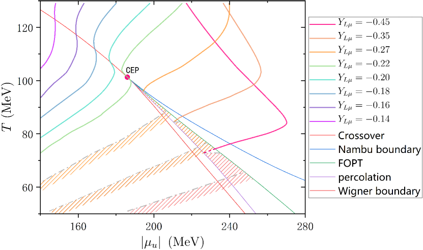
Under the conditions of the kinetic and the chemical equilibrium Schwarz and Stuke (2009), the net leptons and the photons number densities are expressed by Fermi-Dirac distributions and Bose-Einstein distributions, respectively. In the QCD sector, the nonperturbative property prevents the QCD matter from being simply represented by Fermi-Dirac and Bose-Einstein distributions. Therefore, we apply the DSE to accomplish the complete calculations of the QCD phase diagram, the thermodynamic quantities and especially here the effective potential, which is for the first time obtained and applied to compute the gravitational wave signals. Firstly, in the current scheme one obtains the critical end point (CEP) at Zheng et al. (2024). Moreover, with the effective potential obtained from the homotopy method, it is able to determine the first-order phase transition (FOPT) line, on which the chiral symmetric (Wigner) phase and the chiral symmetry breaking (Nambu) phase degenerate.
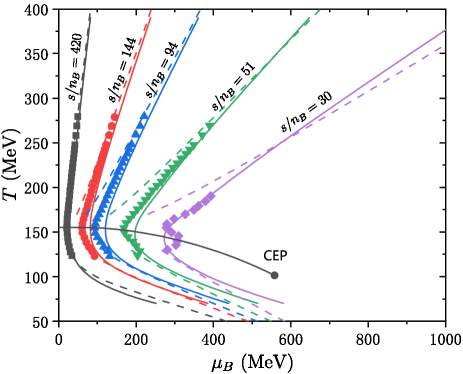
The scenario () is the main focus of this work, which satisfies the BBN constraints and can induce the FOPT of QCD Middeldorf-Wygas et al. (2022); Gao and Oldengott (2022). In this scenario, Fig. 1 illustrates the dependence of cosmic trajectory on , where represents the critical value to trigger the FOPT, which is consistent with the previous study Gao et al. (2023). As decreases gradually from to , the cosmic trajectory quickly approaches to CEP, which is caused by the strengthening of PT as approaching CEP. When , the cosmic trajectory steps into the FOPT region.
When the cosmic trajectory crosses the QCD FOPT, there can be GW emission during the bubble nucleation. This is a non-equilibrium process which includes the false-vacuum-dominated stage and the supercooling stage, represented by the solid line and the dashed line respectively in Fig. 1. Before the nucleation, the dynamics can be studied with the QCD effective potential at hand, which will be explained in detail in the next section. After the nucleation, when the part of the Universe is converted to the true vacuum, the entropy of the system is not conserved anymore due to the non-equilibrium effect. The upper bound of the cosmic trajectory, i.e., the gray dot-dashed line below, is determined under the condition that is conserved after the PT as depicted in Fig. 1. However, the complete determination requires to further consider the dynamics of the FOPT which is under progress. A detailed illustration of the evolution of the cosmic trajectory is presented in the supplemental material.
PT parameters.
With the mechanism of the QCD FOPT, one can expect the generation of the GWs. We consider the sound-waves-only analysis (PT-SOUND) for the GW because our subsequent calculation shows that the bubble walls cannot runaway. The PT-SOUND GW spectrum is written as Afzal et al. (2023); Jinno and Takimoto (2017); Hindmarsh et al. (2015); Espinosa et al. (2010); Ellis et al. (2020, 2019a); Guo et al. (2021); Weir (2018):
| (2) |
with the PT strength, being the inverse PT duration Espinosa et al. (2010) and the bubble wall velocity. Both of the PT parameters requires the knowledge of the QCD effective potential, which we obtain for the first time by applying the homotopy method to the QCD theory Zheng et al. (2024). Besides, the GWs are always generated along the percolation line, which corresponds to the percolation temperature , i.e., the temperature when of the volume of the universe is converted into the true vacuum determined with the effective potential. These information allows us to obtain the GW spectrum.
The QCD effective potential comes from a generalized Legendre transformation to the Cornwall, Jackiw and Tomboulis (CJT) connected generating functional Zheng et al. (2024). This transformation converts the variable of the CJT effective potential, i.e., the quark propagator, to the self-energy, which is the key point to keep the effective potential to be bounded from below Haymaker et al. (1987). The new effective potential is written as Zheng et al. (2024):
| (3) |
with the free quark propagator, the dressed quark propagator, the self-energy, the external source, and the sum of all two-particle-irreducible diagrams as a functional of .
Moreover, we apply the homotopy method, i.e., a simplified version of the functional integration, to determine the effective potential from the quantitative truncation scheme of the DSE Zheng et al. (2024):
| (4) |
where
| (5) |
with being the homotopy parameter, and being the Wigner and Nambu solutions respectively. Moreover, the effective potential has been converted to a function of by connecting the homotopy parameter to the dynamic quark mass .
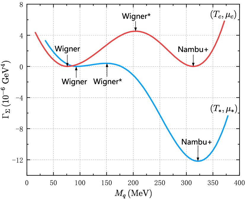
We firstly illustrate the QCD effective potential in Fig. 2, where the Wigner vacuum is the false vacuum, the Nambu is the true vacuum and the Wigner is the unstable vacuum indicating the occurrence of FOPT. At the PT temperature , the false and the true vacuum are degenerate. Vacuum bubbles merge with each other around the percolation temperature . At that time, the false vacuum has an energy larger than the true vacuum.
Using the effective potential, we calculate the decay rate of the false vacuum and find that it is dominated by the thermally-induced decay rate Coleman (1977); Linde (1981, 1983); Ellis et al. (2019b):
| (6) |
with
| (7) |
Here, is the 3-dimensional Euclidean actions for the -symmetric bounce solutions, is the bubble radius, is the dynamical quark mass, , and is the effective potential calculated from the DSE with the homotopy method Zheng et al. (2024).
The percolation temperature is determined by the following equation:
| (8) |
with varying along the cosmic trajectory, the Hubble parameter, the energy density of the radiation, the energy density when the false and the true vacuum are degenerate, and the bubble wall velocity, where we assume as NANOGrav Afzal et al. (2023). ignores the matter because its energy density is much smaller than that of radiation. The percolation temperature can then be determined by and the cosmic trajectory.
The PT strength depends on the available energy released from the PT, normalized to the energy densities of the background radiation:
| (9) |
with
| (10) | ||||
| (11) |
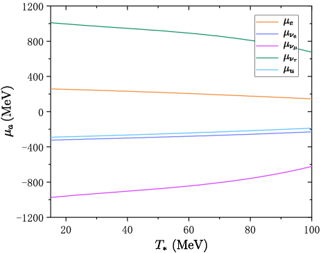
Here, , is the trace anomaly, is the entropy density, is the quark number density, is the pressure where denotes the difference between the false and the true vacuum, and collects electron, muon, all neutrinos, photon and quarks in the false vacuum, where the temperature dependence of the lepton chemical potentials along the percolation line are shown in the Appendix. A critical value that can determine whether the bubble walls can runaway is also considered Ellis et al. (2019a); Bodeker and Moore (2009), which sums over all particles during the PT.
For the FOPT with finite chemical potential, the inverse PT duration can be obtained as:
| (12) |
where the derivative lies along the cosmic trajectory.
Numerical results.
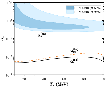
After a complete computation for the GW spectrum, we find that neither of and over the whole QCD chiral PT can be matched with the NANOGrav measurements. This has been depicted clearly in Fig. 3 which gives the comparison between the PT parameters calculated from the QCD effective potential and the sound-wave-only analysis (PT-SOUND) by the NANOGrav collaboration. Note that we only consider the sound-wave-only case because is verified here. This situation prevents the runaway of bubble wave, causing the GW to be dominated by the sound waves source Caprini et al. (2016).
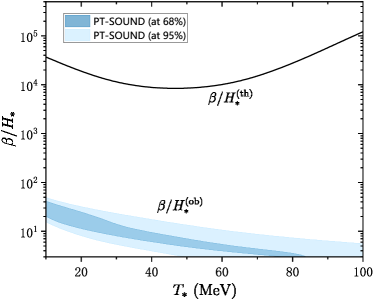
In detail, for , its value is at least one order of magnitude smaller comprared to the NANOGrav constraints. Such a small value is mainly due to the large energy density of the background radiation. The large energy density comes from the large chemical potentials of the leptons, which is a direct result of the conservation conditions in Eq. (1). In particular, the chemical potentials of the electron and electron neutrino are roughly equivalent to that of the quark, while the chemical potentials of muon neutrinos and/or tau neutrinos are more than three times the quark chemical potential. For , the value we obtained is three orders of magnitude larger than the one to match with the analysis from NANOGrav collaboration. This is mainly because the cosmic trajectory leans more towards the chemical potential, causing the derivative of along the trajectory to be large. Meanwhile, in the Eq. (12), outside of the derivative also maintains a large value due to the contribution of the non-vanishing chemical potential along the percolation line. As a result, remains significantly large.
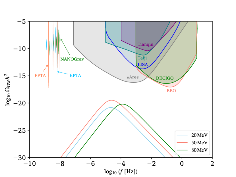
Based on the obtained PT parameters and , we show our result of the GWs sourced from the first-order QCD PT in Fig. 4. The quantitative computation here disapproves the QCD chiral PT as a source of the SGWB to explain the signals detected by NANOGrav.
Conclusion.
In this Letter, we calculate the cosmic trajectories at large quark chemical potential, and for the first time quantitatively determine the PT parameters of the first-order QCD phase transitions, through their relation to the thermodynamic quantities and effective potential from the functional QCD methods.
We firstly verify that a large lepton asymmetry can induce the first-order QCD PT. We consider the scenario (), and find that the FOPT occurs when . This conclusion is essentially from the conservation laws during the Universe evolution without further assumptions. We further compute the PT parameters via the QCD effective potential, and then determine the gravitational wave spectrum through the sound shell model.
The obtained GW spectrum makes it possible to conduct a quantitative analysis with the measurements of NANOGrav. In short, the obtained PT strength is , the inverse PT duration is . The values deviate significantly from the measurements of NANOGrav mainly due to the large energy density of the background radiation. This large energy density arises from the large chemical potentials of the leptons, which is a direct result of the conservation laws.
Finally, we illustrate the disparity between the computed GW spectra based on the PT parameters and the violin plots of the EPTA, PPTA and NANOGrav, alongside the sensitivity curves of the Ares, Taiji, Tianqin, LISA, BBO and DECIGO. In brief, through a quantitative determination of the QCD PT parameters, we find that a first-order chiral PT of QCD cannot produce the SGWB signal by the NANOGrav experiment. The PT is also too weak to produce detectable GW signals that can be reached by the current and the being constructed GW detectors.
Acknowledgements.
Acknowledgments
F.G. and H.Z. thank Isabel M. Oldengott and Yi Lu for helpful discussions. This work is supported by the National Science Foundation of China under Grants No.12175007, No.12247107 and No.12305134. L.B. is supported by the National Natural Science Foundation of China (NSFC) under Grants No. 12075041, No. 12322505, and No. 12347101. L.B. also acknowledges Chongqing Talents: Exceptional Young Talents Project No. cstc2024ycjh-bgzxm0020.
References
- Sesana et al. (2021) A. Sesana et al., Exper. Astron. 51, 1333 (2021), arXiv:1908.11391 [astro-ph.IM] .
- Hu and Wu (2017) W.-R. Hu and Y.-L. Wu, Natl. Sci. Rev. 4, 685 (2017).
- Ruan et al. (2020) W.-H. Ruan, Z.-K. Guo, R.-G. Cai, and Y.-Z. Zhang, Int. J. Mod. Phys. A 35, 2050075 (2020), arXiv:1807.09495 [gr-qc] .
- Luo et al. (2016) J. Luo et al. (TianQin), Class. Quant. Grav. 33, 035010 (2016), arXiv:1512.02076 [astro-ph.IM] .
- Zhou et al. (2023) K. Zhou, J. Cheng, and L. Ren, (2023), arXiv:2306.14439 [gr-qc] .
- Amaro-Seoane et al. (2017) P. Amaro-Seoane et al. (LISA), (2017), arXiv:1702.00786 [astro-ph.IM] .
- Baker et al. (2019) J. Baker et al., (2019), arXiv:1907.06482 [astro-ph.IM] .
- Crowder and Cornish (2005) J. Crowder and N. J. Cornish, Phys. Rev. D 72, 083005 (2005), arXiv:gr-qc/0506015 .
- Corbin and Cornish (2006) V. Corbin and N. J. Cornish, Class. Quant. Grav. 23, 2435 (2006), arXiv:gr-qc/0512039 .
- Harry et al. (2006) G. M. Harry, P. Fritschel, D. A. Shaddock, W. Folkner, and E. S. Phinney, Class. Quant. Grav. 23, 4887 (2006), [Erratum: Class.Quant.Grav. 23, 7361 (2006)].
- Seto et al. (2001) N. Seto, S. Kawamura, and T. Nakamura, Phys. Rev. Lett. 87, 221103 (2001), arXiv:astro-ph/0108011 .
- Kawamura et al. (2006) S. Kawamura et al., Class. Quant. Grav. 23, S125 (2006).
- Yagi and Seto (2011) K. Yagi and N. Seto, Phys. Rev. D 83, 044011 (2011), [Erratum: Phys.Rev.D 95, 109901 (2017)], arXiv:1101.3940 [astro-ph.CO] .
- Isoyama et al. (2018) S. Isoyama, H. Nakano, and T. Nakamura, PTEP 2018, 073E01 (2018), arXiv:1802.06977 [gr-qc] .
- Arzoumanian et al. (2020) Z. Arzoumanian et al. (NANOGrav), Astrophys. J. Lett. 905, L34 (2020), arXiv:2009.04496 [astro-ph.HE] .
- Agazie et al. (2023a) G. Agazie et al. (NANOGrav), Astrophys. J. Lett. 951, L8 (2023a), arXiv:2306.16213 [astro-ph.HE] .
- Chen et al. (2021) S. Chen et al. (EPTA), Mon. Not. Roy. Astron. Soc. 508, 4970 (2021), arXiv:2110.13184 [astro-ph.HE] .
- Antoniadis et al. (2023) J. Antoniadis et al. (EPTA, InPTA:), Astron. Astrophys. 678, A50 (2023), arXiv:2306.16214 [astro-ph.HE] .
- Goncharov et al. (2021) B. Goncharov et al., Astrophys. J. Lett. 917, L19 (2021), arXiv:2107.12112 [astro-ph.HE] .
- Reardon et al. (2023a) D. J. Reardon et al., Astrophys. J. Lett. 951, L6 (2023a), arXiv:2306.16215 [astro-ph.HE] .
- Antoniadis et al. (2022) J. Antoniadis et al., Mon. Not. Roy. Astron. Soc. 510, 4873 (2022), arXiv:2201.03980 [astro-ph.HE] .
- Xu et al. (2023) H. Xu et al., Res. Astron. Astrophys. 23, 075024 (2023), arXiv:2306.16216 [astro-ph.HE] .
- Rajagopal and Romani (1995) M. Rajagopal and R. W. Romani, Astrophys. J. 446, 543 (1995), arXiv:astro-ph/9412038 .
- Phinney (2001) E. S. Phinney, (2001), arXiv:astro-ph/0108028 .
- Jaffe and Backer (2003) A. H. Jaffe and D. C. Backer, Astrophys. J. 583, 616 (2003), arXiv:astro-ph/0210148 .
- Wyithe and Loeb (2003) J. S. B. Wyithe and A. Loeb, Astrophys. J. 590, 691 (2003), arXiv:astro-ph/0211556 .
- Ananda et al. (2007) K. N. Ananda, C. Clarkson, and D. Wands, Phys. Rev. D 75, 123518 (2007), arXiv:gr-qc/0612013 .
- Baumann et al. (2007) D. Baumann, P. J. Steinhardt, K. Takahashi, and K. Ichiki, Phys. Rev. D 76, 084019 (2007), arXiv:hep-th/0703290 .
- Losada (1997) M. Losada, Phys. Rev. D 56, 2893 (1997), arXiv:hep-ph/9605266 .
- Cline and Lemieux (1997) J. M. Cline and P.-A. Lemieux, Phys. Rev. D 55, 3873 (1997), arXiv:hep-ph/9609240 .
- Laine (1996) M. Laine, Nucl. Phys. B 481, 43 (1996), [Erratum: Nucl.Phys.B 548, 637–638 (1999)], arXiv:hep-ph/9605283 .
- Bodeker et al. (1997) D. Bodeker, P. John, M. Laine, and M. G. Schmidt, Nucl. Phys. B 497, 387 (1997), arXiv:hep-ph/9612364 .
- Neronov et al. (2021) A. Neronov, A. Roper Pol, C. Caprini, and D. Semikoz, Phys. Rev. D 103, 041302 (2021), arXiv:2009.14174 [astro-ph.CO] .
- Li et al. (2021) S. L. Li, L. J. Shao, P. X. Wu, and H. Yu, Phys. Rev. D 104, 043510 (2021), arXiv:2101.08012 [astro-ph.CO] .
- Nakai et al. (2021) Y. Nakai, M. Suzuki, F. Takahashi, and M. Yamada, Phys. Lett. B 816, 136238 (2021), arXiv:2009.09754 [astro-ph.CO] .
- Ratzinger and Schwaller (2021) W. Ratzinger and P. Schwaller, SciPost Phys. 10, 047 (2021), arXiv:2009.11875 [astro-ph.CO] .
- Kosowsky et al. (1992) A. Kosowsky, M. S. Turner, and R. Watkins, Phys. Rev. Lett. 69, 2026 (1992).
- Caprini et al. (2010) C. Caprini, R. Durrer, and X. Siemens, Phys. Rev. D 82, 063511 (2010), arXiv:1007.1218 [astro-ph.CO] .
- Addazi et al. (2021) A. Addazi, Y.-F. Cai, Q. Gan, A. Marciano, and K. Zeng, Sci. China Phys. Mech. Astron. 64, 290411 (2021), arXiv:2009.10327 [hep-ph] .
- Xue et al. (2021) X. Xue et al., Phys. Rev. Lett. 127, 251303 (2021), arXiv:2110.03096 [astro-ph.CO] .
- Ellis et al. (2023) J. Ellis, M. Lewicki, C. Lin, and V. Vaskonen, Phys. Rev. D 108, 103511 (2023), arXiv:2306.17147 [astro-ph.CO] .
- Addazi et al. (2024) A. Addazi, Y.-F. Cai, A. Marciano, and L. Visinelli, Phys. Rev. D 109, 015028 (2024), arXiv:2306.17205 [astro-ph.CO] .
- Ghosh et al. (2024) T. Ghosh, A. Ghoshal, H.-K. Guo, F. Hajkarim, S. F. King, K. Sinha, X. Wang, and G. White, JCAP 05, 100 (2024), arXiv:2307.02259 [astro-ph.HE] .
- Rezapour et al. (2022a) S. Rezapour, K. Bitaghsir Fadafan, and M. Ahmadvand, Annals Phys. 437, 168731 (2022a), arXiv:2006.04265 [hep-th] .
- Rezapour et al. (2022b) S. Rezapour, K. Bitaghsir Fadafan, and M. Ahmadvand, Phys. Scripta 97, 035301 (2022b).
- Ahmadvand and Bitaghsir Fadafan (2018) M. Ahmadvand and K. Bitaghsir Fadafan, Phys. Lett. B 779, 1 (2018), arXiv:1707.05068 [hep-th] .
- Ahmadvand and Bitaghsir Fadafan (2017) M. Ahmadvand and K. Bitaghsir Fadafan, Phys. Lett. B 772, 747 (2017), arXiv:1703.02801 [hep-th] .
- Athron et al. (2024) P. Athron, A. Fowlie, C.-T. Lu, L. Morris, L. Wu, Y. Wu, and Z. Xu, Phys. Rev. Lett. 132, 221001 (2024), arXiv:2306.17239 [hep-ph] .
- Han et al. (2023) C. Han, K.-P. Xie, J. M. Yang, and M. Zhang, (2023), arXiv:2306.16966 [hep-ph] .
- Li and Xie (2023) S.-P. Li and K.-P. Xie, Phys. Rev. D 108, 055018 (2023), arXiv:2307.01086 [hep-ph] .
- Siemens et al. (2007) X. Siemens, V. Mandic, and J. Creighton, Phys. Rev. Lett. 98, 111101 (2007), arXiv:astro-ph/0610920 .
- Ellis and Lewicki (2021) J. Ellis and M. Lewicki, Phys. Rev. Lett. 126, 041304 (2021), arXiv:2009.06555 [astro-ph.CO] .
- Blasi et al. (2021) S. Blasi, V. Brdar, and K. Schmitz, Phys. Rev. Lett. 126, 041305 (2021), arXiv:2009.06607 [astro-ph.CO] .
- Buchmuller et al. (2020) W. Buchmuller, V. Domcke, and K. Schmitz, Phys. Lett. B 811, 135914 (2020), arXiv:2009.10649 [astro-ph.CO] .
- Lazarides et al. (2023) G. Lazarides, R. Maji, and Q. Shafi, Phys. Rev. D 108, 095041 (2023), arXiv:2306.17788 [hep-ph] .
- Wang et al. (2023) Z. Wang, L. Lei, H. Jiao, L. Feng, and Y.-Z. Fan, Sci. China Phys. Mech. Astron. 66, 120403 (2023), arXiv:2306.17150 [astro-ph.HE] .
- Samanta and Datta (2021) R. Samanta and S. Datta, JHEP 05, 211 (2021), arXiv:2009.13452 [hep-ph] .
- Bian et al. (2022a) L. Bian, J. Shu, B. Wang, Q. Yuan, and J. Zong, Phys. Rev. D 106, L101301 (2022a), arXiv:2205.07293 [hep-ph] .
- Hiramatsu et al. (2014) T. Hiramatsu, M. Kawasaki, and K. Saikawa, JCAP 02, 031 (2014), arXiv:1309.5001 [astro-ph.CO] .
- Bian et al. (2021) L. Bian, R.-G. Cai, J. Liu, X.-Y. Yang, and R. Zhou, Phys. Rev. D 103, L081301 (2021), arXiv:2009.13893 [astro-ph.CO] .
- Ferreira et al. (2023) R. Z. Ferreira, A. Notari, O. Pujolas, and F. Rompineve, JCAP 02, 001 (2023), arXiv:2204.04228 [astro-ph.CO] .
- Bai et al. (2023) Y. Bai, T.-K. Chen, and M. Korwar, JHEP 12, 194 (2023), arXiv:2306.17160 [hep-ph] .
- Kitajima et al. (2024) N. Kitajima, J. Lee, K. Murai, F. Takahashi, and W. Yin, Phys. Lett. B 851, 138586 (2024), arXiv:2306.17146 [hep-ph] .
- Blasi et al. (2023) S. Blasi, A. Mariotti, A. Rase, and A. Sevrin, JHEP 11, 169 (2023), arXiv:2306.17830 [hep-ph] .
- Li et al. (2023) Y. Li, L. Bian, and Y. Jia, (2023), arXiv:2304.05220 [hep-ph] .
- Bian et al. (2022b) L. Bian, S. Ge, C. Li, J. Shu, and J. Zong, (2022b), arXiv:2212.07871 [hep-ph] .
- Babichev et al. (2023) E. Babichev, D. Gorbunov, S. Ramazanov, R. Samanta, and A. Vikman, Phys. Rev. D 108, 123529 (2023), arXiv:2307.04582 [hep-ph] .
- Sakharov et al. (2021) A. S. Sakharov, Y. N. Eroshenko, and S. G. Rubin, Phys. Rev. D 104, 043005 (2021), arXiv:2104.08750 [hep-ph] .
- Zhang et al. (2023) Z. Zhang, C. Cai, Y.-H. Su, S. Wang, Z.-H. Yu, and H.-H. Zhang, Phys. Rev. D 108, 095037 (2023), arXiv:2307.11495 [hep-ph] .
- Afzal et al. (2023) A. Afzal et al. (NANOGrav), Astrophys. J. Lett. 951, L11 (2023), arXiv:2306.16219 [astro-ph.HE] .
- Bian et al. (2024) L. Bian, S. Ge, J. Shu, B. Wang, X.-Y. Yang, and J. Zong, Phys. Rev. D 109, L101301 (2024), arXiv:2307.02376 [astro-ph.HE] .
- Bai and Korwar (2022) Y. Bai and M. Korwar, Phys. Rev. D 105, 095015 (2022), arXiv:2109.14765 [hep-ph] .
- Gao and Oldengott (2022) F. Gao and I. M. Oldengott, Phys. Rev. Lett. 128, 131301 (2022), arXiv:2106.11991 [hep-ph] .
- Gao et al. (2023) F. Gao, J. Harz, C. Hati, Y. Lu, I. M. Oldengott, and G. White, (2023), arXiv:2309.00672 [hep-ph] .
- Lu et al. (2023a) Y. Lu, F. Gao, Y. X. Liu, and J. M. Pawlowski, (2023a), to appear in Phys. Rev. D, arXiv:2310.18383 [hep-ph] .
- Zheng et al. (2024) H. W. Zheng, Y. Lu, F. Gao, S. X. Qin, and Y. X. Liu, Phys. Rev. D 109, 114013 (2024), arXiv:2312.00382 [hep-ph] .
- Roberts and Williams (1994) C. D. Roberts and A. G. Williams, Prog. Part. Nucl. Phys. 33, 477 (1994), arXiv:hep-ph/9403224 .
- Roberts and Schmidt (2000) C. D. Roberts and S. M. Schmidt, Prog. Part. Nucl. Phys. 45, S1 (2000), arXiv:nucl-th/0005064 .
- Alkofer and von Smekal (2001) R. Alkofer and L. von Smekal, Phys. Rept. 353, 281 (2001), arXiv:hep-ph/0007355 .
- Fischer (2006) C. S. Fischer, J. Phys. G 32, R253 (2006), arXiv:hep-ph/0605173 .
- Gao et al. (2021) F. Gao, J. Papavassiliou, and J. M. Pawlowski, Phys. Rev. D 103, 094013 (2021), arXiv:2102.13053 [hep-ph] .
- Gao and Pawlowski (2020) F. Gao and J. M. Pawlowski, Phys. Rev. D 102, 034027 (2020), arXiv:2002.07500 [hep-ph] .
- Gunkel and Fischer (2021) P. J. Gunkel and C. S. Fischer, Phys. Rev. D 104, 054022 (2021), arXiv:2106.08356 [hep-ph] .
- Schwarz and Stuke (2009) D. J. Schwarz and M. Stuke, JCAP 11, 025 (2009), [Erratum: JCAP 10, E01 (2010)], arXiv:0906.3434 [hep-ph] .
- Aghanim et al. (2020) N. Aghanim et al. (Planck), Astron. Astrophys. 641, A6 (2020), [Erratum: Astron.Astrophys. 652, C4 (2021)], arXiv:1807.06209 [astro-ph.CO] .
- Pitrou et al. (2018) C. Pitrou, A. Coc, J. P. Uzan, and E. Vangioni, Phys. Rept. 754, 1 (2018), arXiv:1801.08023 [astro-ph.CO] .
- Oldengott and Schwarz (2017) I. M. Oldengott and D. J. Schwarz, EPL 119, 29001 (2017), arXiv:1706.01705 [astro-ph.CO] .
- Popa and Vasile (2008) L. A. Popa and A. Vasile, JCAP 06, 028 (2008), arXiv:0804.2971 [astro-ph] .
- Simha and Steigman (2008) V. Simha and G. Steigman, JCAP 08, 011 (2008), arXiv:0806.0179 [hep-ph] .
- Serpico and Raffelt (2005) P. D. Serpico and G. G. Raffelt, Phys. Rev. D 71, 127301 (2005), arXiv:astro-ph/0506162 .
- Gelmini et al. (2020) G. B. Gelmini, M. Kawasaki, A. Kusenko, K. Murai, and V. Takhistov, JCAP 09, 051 (2020), arXiv:2005.06721 [hep-ph] .
- Pastor et al. (2009) S. Pastor, T. Pinto, and G. G. Raffelt, Phys. Rev. Lett. 102, 241302 (2009), arXiv:0808.3137 [astro-ph] .
- Mangano et al. (2011) G. Mangano, G. Miele, S. Pastor, O. Pisanti, and S. Sarikas, JCAP 03, 035 (2011), arXiv:1011.0916 [astro-ph.CO] .
- Mangano et al. (2012) G. Mangano, G. Miele, S. Pastor, O. Pisanti, and S. Sarikas, Phys. Lett. B 708, 1 (2012), arXiv:1110.4335 [hep-ph] .
- Middeldorf-Wygas et al. (2022) M. M. Middeldorf-Wygas, I. M. Oldengott, D. Bödeker, and D. J. Schwarz, Phys. Rev. D 105, 123533 (2022), arXiv:2009.00036 [hep-ph] .
- Jinno and Takimoto (2017) R. Jinno and M. Takimoto, Phys. Rev. D 95, 024009 (2017), arXiv:1605.01403 [astro-ph.CO] .
- Hindmarsh et al. (2015) M. Hindmarsh, S. J. Huber, K. Rummukainen, and D. J. Weir, Phys. Rev. D 92, 123009 (2015), arXiv:1504.03291 [astro-ph.CO] .
- Espinosa et al. (2010) J. R. Espinosa, T. Konstandin, J. M. No, and G. Servant, JCAP 06, 028 (2010), arXiv:1004.4187 [hep-ph] .
- Ellis et al. (2020) J. Ellis, M. Lewicki, and J. M. No, JCAP 07, 050 (2020), arXiv:2003.07360 [hep-ph] .
- Ellis et al. (2019a) J. Ellis, M. Lewicki, J. M. No, and V. Vaskonen, JCAP 06, 024 (2019a), arXiv:1903.09642 [hep-ph] .
- Guo et al. (2021) H. K. Guo, K. Sinha, D. Vagie, and G. White, JCAP 01, 001 (2021), arXiv:2007.08537 [hep-ph] .
- Weir (2018) D. J. Weir, Phil. Trans. Roy. Soc. Lond. A 376, 20170126 (2018), [Erratum: Phil.Trans.Roy.Soc.Lond.A 381, 20230212 (2023)], arXiv:1705.01783 [hep-ph] .
- Haymaker et al. (1987) R. W. Haymaker, T. Matsuki, and F. Cooper, Phys. Rev. D 35, 2567 (1987).
- Coleman (1977) S. R. Coleman, Phys. Rev. D 15, 2929 (1977), [Erratum: Phys.Rev.D 16, 1248 (1977)].
- Linde (1981) A. D. Linde, Phys. Lett. B 100, 37 (1981).
- Linde (1983) A. D. Linde, Nucl. Phys. B 216, 421 (1983), [Erratum: Nucl.Phys.B 223, 544 (1983)].
- Ellis et al. (2019b) J. Ellis, M. Lewicki, and J. M. No, JCAP 04, 003 (2019b), arXiv:1809.08242 [hep-ph] .
- Bodeker and Moore (2009) D. Bodeker and G. D. Moore, JCAP 05, 009 (2009), arXiv:0903.4099 [hep-ph] .
- Caprini et al. (2016) C. Caprini et al., JCAP 04, 001 (2016), arXiv:1512.06239 [astro-ph.CO] .
- Reardon et al. (2023b) D. J. Reardon et al., Astrophys. J. Lett. 951, L7 (2023b), arXiv:2306.16229 [astro-ph.HE] .
- Zic et al. (2023) A. Zic et al., Publ. Astron. Soc. Austral. 40, e049 (2023), arXiv:2306.16230 [astro-ph.HE] .
- Agazie et al. (2023b) G. Agazie et al. (NANOGrav), Astrophys. J. Lett. 951, L9 (2023b), arXiv:2306.16217 [astro-ph.HE] .
- Gao et al. (2016) F. Gao, J. Chen, Y. X. Liu, S. X. Qin, C. D. Roberts, and S. M. Schmidt, Phys. Rev. D 93, 094019 (2016), arXiv:1507.00875 [nucl-th] .
- Isserstedt et al. (2019) P. Isserstedt, M. Buballa, C. S. Fischer, and P. J. Gunkel, Phys. Rev. D 100, 074011 (2019), arXiv:1906.11644 [hep-ph] .
- Fu and Pawlowski (2015) W. J. Fu and J. M. Pawlowski, Phys. Rev. D 92, 116006 (2015), arXiv:1508.06504 [hep-ph] .
- Lu et al. (2023b) Y. Lu, F. Gao, B. C. Fu, H. C. Song, and Y. X. Liu, (2023b), arXiv:2310.16345 [hep-ph] .
- Fischer et al. (2014) C. S. Fischer, J. Luecker, and C. A. Welzbacher, Phys. Rev. D 90, 034022 (2014), arXiv:1405.4762 [hep-ph] .
- Philipsen (2013) O. Philipsen, Prog. Part. Nucl. Phys. 70, 55 (2013), arXiv:1207.5999 [hep-lat] .
- Guenther et al. (2017) J. N. Guenther, R. Bellwied, S. Borsanyi, Z. Fodor, S. D. Katz, A. Pasztor, C. Ratti, and K. K. Szabó, Nucl. Phys. A 967, 720 (2017), arXiv:1607.02493 [hep-lat] .
- Eichhorn et al. (2021) A. Eichhorn, J. Lumma, J. M. Pawlowski, M. Reichert, and M. Yamada, JCAP 05, 006 (2021), arXiv:2010.00017 [hep-ph] .
Supplemental Material
I Thermal quantities and Cosmic trajectory during the QCD transition
At finite temperature and chemical potential, the general form of the solution of the quark DSE can be expressed as:
| (13) |
with the momentum, , the Matsubara frequency and the quark chemical potential. Then, the dynamic quark mass is defined as:
| (14) |
The thermal quantities of QCD, including the number density and the entropy density, can be obtained by solving DSE Gao et al. (2016); Isserstedt et al. (2019); Lu et al. (2023a). The quark number density and the entropy can be written as:
| (15) | ||||
| (16) |
with the pressure and the quark chemical potential. The number density of and quark can be expressed in terms of the dynamical quark mass and the traced Polyakov loop in phase diagram () plane Fu and Pawlowski (2015); Lu et al. (2023b):
| (17a) | ||||
| (17b) | ||||
| (17c) | ||||
| (17d) | ||||
with the color number. The traced Polyakov loop at vanishing quark chemical potential is parameterized as Lu et al. (2023b); Fischer et al. (2014):
| (18a) | ||||
| (18b) | ||||
| (18c) | ||||
where the PT temperature at vanishing chemical potential and the curvature of the transition line. The fit parameters are . From the definition of the Eq. (15) and the Eq. (16), the chemical potential dependence of the entropy density can be expressed as the integral along Lu et al. (2023a):
| (19) |
To include the gluon pressure, we use the lattice QCD results to obtain the entropy density at vanishing chemical potential as parametrized in the lattice QCD Philipsen (2013). The full entropy density can then be expressed as:
| (20) |
We compare the isentropic trajectories from DSE with the result of the improved ideal quark gas, HRG and the lattice in Fig. (5), showing an well consistency. The improved ideal quark gas includes the lattice QCD entropy in Eq. (20), and apply the Fermi-Dirac distribution for the quark number densities. The application of is due to the gluons do not behave like the idea gas in the QCD phase transition region. The consistency shown in Fig. (5) makes the calculation of the five conserve equations in Eq. (1) of the cosmic trajectories more reliable, because these equations also satisfies a form similar to .
During the cosmic QCD transition, the kinetic and the chemical equilibrium are excellent approximation Eichhorn et al. (2021). The process is the primary mechanism, responsible for establishing both kinetic and chemical equilibrium among all particles, which constrains the chemical potentials of leptons as , and the leptons and quarks as . Chemical equilibrium constrains the chemical potentials of different particle species to only five independent chemical potentials for the universe. The chemical potentials of photons and gluons are zero because the numbers of photons and gluons are not conserved. The chemical potentials of particles and antiparticles are equal in magnitude, but opposite in sign. For instance, if a particle has a chemical potential of , its antiparticle has a chemical potential of . Due to flavor mixing, we only need to distinguish the chemical potentials of up and down quarks: , and Schwarz and Stuke (2009). Therefore we are left with as the independent variables for the cosmic trajectory. Then the chemical potentials of conserved charges () can be expressed in terms of particle chemical potential as:
| (21a) | ||||
| (21b) | ||||
| (21c) | ||||
Then the temperature dependence of the five chemical potentials () are the cosmic trajectory. We will focus on the () plane in QCD phase diagram, especially in the first-order phase transition region, where the CEP locates at .
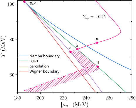
In the scenario (), for a specific value, such as , the cosmic trajectory follows a path from to , crossing the QCD FOPT region illustrated in Fig. 6. During the - period, the false vacuum energy of the universe is lower, rendering the false vacuum more stable. At this stage, the universe is filled with the false vacuum, which is also referred to as the Wigner vacuum in QCD. In the subsequent - period, the energy of the false vacuum exceeds that of the true vacuum, yet both are in local minima. During this period, the false vacuum is a supercooled phase, meaning the universe remaining filled with the false vacuum. At the point , the false vacuum initiates the decay into the true vacuum, leading to the nucleation and the percolation of bubbles. The - process remains unclear, since the non-equilibrium processes are not calculated currently, while the cosmic trajectories involving the non-equilibrium processes can be constrained within the shadow area. This shadowed area is bounded by an upper limit but remains unconstrained by a lower limit. The dot-dashed line above the point represents the upper bound of the cosmic trajectory. This upper bound is calculated under the conservation of before and after the phase transition, while could increase in general through the non-equilibrium processes. This upper bound is determined by the thermal quantities of the true vacuum. As one approaches the point , the Gibbs phase equilibrium condition requires the cosmic trajectory aligns with the FOPT line. At the point , the universe is filled with the true vacuum just at this moment. During the process from the point to , quarks gain a large mass due to the dynamic chiral symmetry breaking, which then suppresses the quark number density of the true vacuum, rendering the cosmic trajectory to be shifted below that of the false vacuum.
II PT parameters of gravitational waves at finite temperature and chemical potential
A critical value of , which can determine whether the bubble walls can runaway, is defined as Ellis et al. (2019a):
| (22) |
where Bodeker and Moore (2009)
| (23) |
with summing over all particles taking part in the phase transition, () the particle mass in false (true) vacuum and the Fermi–Dirac (Bose–Einstein) distribution function.
To obtain the PT parameters that take the derivative along the cosmic trajectory at finite temperature and chemical potential, we start with the fluid equation:
| (24) |
with
| (25) |
with the scale factor, the energy density of radiation and the pressure. Eq. (25) is valid even for radiation in finite chemical potential. The term considers only the radiation (except for muon due to its mass is close to the PT temperature), because the matter energy density is much smaller than that of the radiation. The quarks in the false vacuum, instead of the true vacuum, are considered in because the decay rate is that of the false vacuum. Combining Eq. (24) and Eq. (25), we obtain:
| (26) | ||||
| (27) |
with the time along the cosmic trajectory, the Hubble parameter and the energy density at a given time.
The probability that a point still remains in the false vacuum is written as Ellis et al. (2019b):
| (28) | ||||
| (29) |
After that, the formula to determine the percolation temperature and chemical potential can be derived by applying Eq. (26) and Eq. (27) to Eq. (29):
| (30) |
Similarly, the inverse PT duration can be derived with Eq. (26):
| (31) |
where the derivative lies along the cosmic trajectory.