A Preconditioned Discontinuous Galerkin Method for Biharmonic Equation with $C^{0}$-Reconstructed Approximation

Abstract.

In this paper, we present a high-order finite element method based on a reconstructed approximation to the biharmonic equation. In our construction, the space is reconstructed from nodal values by solving a local least squares fitting problem per element. It is shown that the space can achieve an arbitrarily high-order accuracy and share the same nodal degrees of freedom with the $C^{0}$ linear space. The interior penalty discontinuous Galerkin scheme can be directly applied to the reconstructed space for solving the biharmonic equation. We prove that the numerical solution converges with optimal orders under error measurements. More importantly, we establish a norm equivalence between the reconstructed space and the continuous linear space. This property allows us to precondition the linear system arising from the high-order scheme by the continuous linear space on the same mesh. This preconditioner is shown to be optimal in the sense that the condition number of the preconditioned system admits a uniform upper bound independent of the mesh size. Numerical examples in two and three dimensions are provided to illustrate the accuracy of the scheme and the efficiency of the preconditioning method.

keywords: reconstructed approximation; least squares fitting; interior penalty discontinuous Galerkin method; low-order preconditioning; multigrid method;

1. Introduction

The biharmonic equation is a fourth-order elliptic equation arising in fields of continuum mechanics. It models the thin plate bending problem in continuum mechanics and describes the slow flows of viscous incompressible fluids. For numerically solving the biharmonic equation, finite element method has been a standard numerical technique, and till now, there are many successful finite element methods for this problem, known as conforming, non-conforming and mixed methods.

Conforming methods use $C^{1}$ elements in the scheme, which satisfy the $C^{1}$ continuity conditions across interelement boundaries; see [2, 16, 14]. The implementation of such elements and spaces is quite complicated even in two dimensions. The non-conforming methods relax the strong continuity requirements across the interelement faces and avoid the construction of $C^{1}$ elements; we refer to [1, 32, 40, 41] for some typical elements. The construction of such elements with high-order polynomials is also non-trivial, and they are rarely used in practice. The mixed finite element method (see [4] and the references therein) is another standard method in solving the biharmonic equation, which also avoids using $C^{1}$ elements. The fourth-order equation is rewritten into a system of second-order elliptic equations, and the mixed system can be solved with $C^{0}$ spaces. The mixed method introduces an auxiliary variable, which increases the number of unknowns and leads to a saddle point linear system. In recent years, the discontinuous Galerkin (DG) finite element methods and the $C^{0}$ interior penalty methods have been developed for the biharmonic equation; see [33, 45, 34, 19, 15, 22] for DG methods and see [17, 8, 7] for $C^{0}$ interior penalty methods. Both methods can also be regarded as non-conforming methods. The $C^{1}$ continuity conditions are weakly imposed by applying proper penalties on the interelement faces in the bilinear form. Consequently, simple finite element spaces such as discontinuous piecewise polynomial spaces and $C^{0}$ Lagrange finite element spaces can be used to solve the biharmonic equation. The elements in both spaces are much simpler than $C^{1}$ elements especially when using high-order polynomials. In addition, the DG methods allow totally discontinuous elements, which provide great flexibility in the mesh partition but introduce more degrees of freedom than $C^{0}$ spaces. To achieve a high-order accuracy, an alternative approach is to apply some reconstruction techniques in the scheme, which may give a better approximation but with less degrees of freedom. In [27, 13, 23, 24], the recovery based methods were developed and analysed, which solved the biharmonic equation by $C^{0}$ linear elements. The main idea of such methods is to employ a gradient recovery operator to reconstruct the piecewise constant gradient as a piecewise linear function. Then, computing the second-order derivatives for $C^{0}$ linear finite element functions becomes possible. In [29, 30], the authors proposed a reconstructed finite element method to the biharmonic equation, where the high-order approximation space was obtained by a patch reconstruction process from the piecewise constant space. The idea of reconstructing high-order spaces from low-order spaces in solving the fourth-order equation can be traced back to the works on developing plate and shell elements; see [36, 38].

In this work, we extend the idea of the reconstructed method in [30] to the biharmonic equation. The high-order approximation space is reconstructed from the $C^{0}$ linear space, i.e. only nodal degrees of freedom are involved. For each element, we construct a wide patch and solve a local least squares fitting problem from nodal degrees of freedom in the patch to seek a high-order polynomial. We prove that any high-order accuracy can be achieved by the reconstructed space while the space shares the same degrees of freedom with the continuous linear space. The new space consists of discontinuous piecewise polynomial functions, and can be regraded as a small subspace of the standard discontinuous piecewise polynomial space. Thus, it is natural to employ the interior penalty discontinuous Galerkin scheme to the reconstructed space for solving the biharmonic equation, and the error estimation is also straightforward under the Lax-Milgram framework. We prove the optimal convergence rates under error measurements, which are also confirmed by a series of numerical tests in two and three dimensions.

For the fourth-order equation, solving the resulting linear system efficiently is of particular concern in finite element methods because the final matrix is extremely ill-conditioned, which, generally, has a condition number of $O(h^{-4})$. Therefore, it is very desired to develop an efficient linear solver. The most common methods are to construct a proper preconditioner, which can remarkably reduce the condition number in the preconditioned system, such as multigrid methods and domain decomposition methods. For classical conforming and non-conforming elements, the preconditioning methods have been well developed; see [50, 49, 6, 5, 46, 44, 11]. As mentioned in [25], there are few works concerning the preconditioning techniques for the penalty methods. In [25, 18], the authors presented two-level non-overlapping and overlapping additive Schwarz methods for DG methods, where the bound of the condition number to the preconditioned system was given. In [42, 43], the authors developed the non-overlapping domain decomposition method for DG methods solving HJB equations. For $C^{0}$ interior penalty methods, we refer to [10] and [9] for the two-level Schwarz method and the multigrid method, respectively. For the proposed method, the main feature is that the reconstructed space uses only nodal degrees of freedom to achieve a high-order accuracy. From this fact, we can show that the inverse of the matrix arising from the lowest-order scheme, i.e. the scheme over the continuous linear spaces, can serve as a preconditioner to any high-order reconstructed space on the same mesh. The low-order preconditioning is also a classical technique in finite element methods for preconditioning the high-order scheme; see [12, 37, 28] for some examples. We establish a norm equivalence between the reconstructed space and the continuous linear space. This crucial property allows us to prove that the preconditioner is optimal by showing the condition number of the preconditioned system admits a upper bound independent of the mesh size. Moreover, we propose a multigrid method as an approximation to the inverse of the matrix from the lowest-order scheme, following the idea in [47]. The convergence analysis to the multigrid method is also presented. The numerical tests in two and three dimensions illustrate the efficiency of the preconditioning method.

The rest of this paper is organized as follows. In Section 2, we give some notation used in the scheme. In Section 3, we introduce the reconstructed approximation space and prove the basic properties of the space. Section 4 presents the interior penalty scheme for the biharmonic equation. The preconditioning method is also proposed and analysed in this section. In Section 5, we conduct a series of numerical tests to demonstrate the accuracy to the proposed scheme and the efficiency to the preconditioning method.

2. Preliminaries

Let $\Omega\subset\mathbb{R}^{d}(d=2,3)$ be a bounded convex polygonal (polyhedral) domain with the boundary $\partial\Omega$. Let $\mathcal{T}_{h}$ be a quasi-uniform triangulation of the domain $\Omega$ into triangular (tetrahedral) elements. For any $K\in\mathcal{T}_{h}$, we let $h_{K}:=\text{diam}(K)$ be its diameter, and let $\rho_{K}$ be the radius of the largest ball inscribed in $K$. We let $h:=\max_{K\in\mathcal{T}_{h}}h_{K}$ and $\rho:=\min_{K\in\mathcal{T}_{h}}\rho_{K}$, where $h$ is also the mesh size. The mesh $\mathcal{T}_{h}$ is assumed to be quasi-uniform in the sense that there exists a constant $C_{\nu}$ independent of $h$ such that $h\leq C_{\nu}\rho$, where $\rho:=\min_{K\in\mathcal{T}_{h}}\rho_{K}$. For any $K\in\mathcal{T}_{h}$, we let $w(K):=\{K^{\prime}\in\mathcal{T}_{h}:\ \overline{K}\cap\overline{K^{\prime}}\neq\varnothing\}$ be the set of elements touching $K$. Let $\mathcal{E}_{h}$ be the set of all $d-1$ dimensional faces in $\mathcal{T}_{h}$, and we decompose $\mathcal{E}_{h}$ into $\mathcal{E}_{h}=\mathcal{E}_{h}^{i}+\mathcal{E}_{h}^{b}$, where $\mathcal{E}_{h}^{i}$ and $\mathcal{E}_{h}^{b}$ are collections of interior faces and the faces lying on the boundary $\partial\Omega$, respectively. For any $e\in\mathcal{E}_{h}$, we let $h_{e}:=\text{diam}(e)$ be its diameter. We further denote by $\mathcal{N}_{h}$ be the set of all nodes in $\mathcal{T}_{h}$. Similarly, $\mathcal{N}_{h}$ is decomposed into $\mathcal{N}_{h}=\mathcal{N}_{h}^{i}+\mathcal{N}_{h}^{b}$, where $\mathcal{N}_{h}^{i}:=\{\boldsymbol{\nu}\in\mathcal{N}_{h}:\ \boldsymbol{\nu}\in\Omega\}$ and $\mathcal{N}_{h}^{b}:=\{\boldsymbol{\nu}\in\mathcal{N}_{h}:\ \boldsymbol{\nu}\in\partial\Omega\}$. For any $K\in\mathcal{T}_{h}$, we define $\mathcal{N}_{K}:=\{\boldsymbol{\nu}\in\mathcal{N}_{h}:\boldsymbol{\nu}\in\partial K\}$ as the set of all vertices of the element $K$.

Next, we introduce the jump and the average operators, which are commonly used in the discontinuous Galerkin framework. Let $e\in\mathcal{E}_{h}^{i}$ be any interior face shared by two neighbouring elements $K^{+}$ and $K^{-}$, i.e. $e=\partial K^{+}\cap\partial K^{-}$, and we let $\boldsymbol{\mathrm{n}}^{+}$ and $\boldsymbol{\mathrm{n}}^{-}$ be the unit outward normal vectors on $e$ corresponding to $K^{+}$ and $K^{-}$, respectively. Let $v$ be a piecewise smooth scalar-valued function, and let $\boldsymbol{q}$ be a piecewise smooth vector- or tensor-valued function, the jump operator $[[\cdot]]$ and the average $\{\cdot\}$ on $e$ are defined as

$$[[v]]|_{e}:=v^{+}|_{e}-v^{-}|_{e},\quad\{v\}|_{e}=\frac{1}{2}(v^{+}|_{e}+v^{-}|_{e}),\quad[[\boldsymbol{q}]]|_{e}:=\boldsymbol{q}^{+}|_{e}-\boldsymbol{q}^{-}|_{e},\quad\{\boldsymbol{q}\}|_{e}=\frac{1}{2}(\boldsymbol{q}^{+}|_{e}+\boldsymbol{q}^{-}|_{e}),$$

where $v^{\pm}:=v|_{K^{\pm}}$, $\boldsymbol{q}^{\pm}:=\boldsymbol{q}|_{K^{\pm}}$. On the boundary face $e\in\mathcal{E}_{h}^{b}$, both operators on $e$ are modified as

$$[[v]]|_{e}:=\{v\}|_{e}:=\tilde{v}|_{e},\quad[[\boldsymbol{q}]]|_{e}:=\{\boldsymbol{q}\}|_{e}:=\tilde{\boldsymbol{q}}|_{e},$$

where $\tilde{v}:=v|_{K}$, $\tilde{\boldsymbol{q}}:=\boldsymbol{q}|_{K}$ with $e\subset\partial K$.

Given an open bounded domain $D\subset\mathbb{R}^{d}$, we let $H^{s}(D)$ denote the usual Sobolev space with the exponent $s\geq 0$, and its associated inner products, seminorms and norms are also followed. Throughout this paper, $C$ and $C$ with subscripts are denoted as generic constants that may vary in different lines but are always independent of $h$.

Our model problem is the following biharmonic equation, which reads

(1) $$\Delta^{2}u =f, \text{in }\Omega,$$

$$u =0, \text{on }\partial\Omega,$$

$$\partial_{\boldsymbol{\mathrm{n}}}u =0, \text{on }\partial\Omega,$$

where $f\in L^{2}(\Omega)$, and $\boldsymbol{\mathrm{n}}$ denotes the unit outward normal vector on the boundary $\partial\Omega$. For simplicity, we assume that the problem (1) possesses a unique solution $u\in H^{4}(\Omega)$. We refer to [3] for more results about the regularity.

3. Reconstruction from $C^{0}$ linear space

In this section, we introduce an approximation space for the problem (1) by presenting a reconstruction procedure on the standard $\mathcal{P}_{1}$ finite element spaces $V_{h}:=\{v_{h}\in H^{1}(\Omega):\ v_{h}|_{K}\in\mathcal{P}_{1}(K),\ \forall K\in\mathcal{T}_{h}\}$ and $V_{h,0}:=V_{h}\cap H_{0}^{1}(\Omega)$. The main idea is to define a linear operator $\mathcal{R}^{m}$ that maps any $v_{h}\in V_{h}$ into a high-order piecewise polynomial function, i.e. its image space will be a piecewise polynomial space. The reconstruction contains two steps: constructing a wide element patch for each element and solving a local least squares fitting problem on each patch.

Step 1. For each $K\in\mathcal{T}_{h}$, we collect some neighbouring elements to form a patch set $\mathcal{S}(K)$, which is carried out by a recursive algorithm. We begin by assigning a constant $N_{m}$ to govern the size of the patch $\mathcal{S}(K)$. The value of $N_{m}$ will be specified later. We define a sequence of sets $\mathcal{S}_{t}(K)$ in a recursive manner, which read

(2) $$\mathcal{S}_{0}(K):=\{K\},\quad\mathcal{S}_{t+1}(K):=\bigcup_{K^{\prime}\in\mathcal{S}_{t}(K)}w(K^{\prime}),\quad t\geq 0.$$

For each $\mathcal{S}_{t}(K)$, we define a corresponding set $\mathcal{I}_{t}(K):=\bigcup_{K^{\prime}\in S_{t}(K)}\mathcal{N}_{K^{\prime}}$, which consists of vertices to all elements in $\mathcal{S}_{t}(K)$. The recursive algorithm (2) stops when the depth $t$ meets the condition $\#\mathcal{I}_{t}(K)<N_{m}\leq\#\mathcal{I}_{t+1}(K)$, and meanwhile the recursive depth is denoted as $t_{K}$. Then, we let $\mathcal{S}(K):=\mathcal{S}_{t}(K)$ and sort the elements in $\mathcal{S}_{t+1}(K)\backslash\mathcal{S}_{t}(K)$ by their distances to $K$, where the distance between two elements is measured by the length of the line connecting their barycenters. After sorting, we add the first $n_{t}$ elements in $\mathcal{S}_{t+1}(K)\backslash\mathcal{S}_{t}(K)$ to the set $\mathcal{S}(K)$ such that $\mathcal{I}(K):=\bigcup_{K^{\prime}\in\mathcal{S}(K)}\mathcal{N}_{K^{\prime}}$ has at least $N_{m}$ nodes. The detailed algorithm to construct $\mathcal{S}(K)$ and $\mathcal{I}(K)$ is presented in Algorithm 1. For the set $\mathcal{S}(K)$, we define its corresponding domain $\mathcal{D}(K):=\text{Int}(\bigcup_{K^{\prime}\in\mathcal{S}(K)}\overline{K^{\prime}})$. By the quasi-uniformity of $\mathcal{T}_{h}$, there holds $h_{\mathcal{D}(K)}\leq Ct_{K}h_{K}$, where $h_{\mathcal{D}(K)}:=\text{diam}(\mathcal{D}(K))$.

Input: The mesh $\mathcal{T}_{h}$ and the threshold $N_{m}$;

Output: $\mathcal{S}(K)$ and $\mathcal{I}(K)$ for all elements;

for $K\in\mathcal{T}_{h}$  do

      set $t=0$, $\mathcal{S}_{0}(K)=\{K\}$, $\mathcal{I}_{0}(K)=\mathcal{N}_{K}$;

       repeat

             let $\mathcal{S}(K)=\mathcal{S}_{t}(K)$;

             construct $\mathcal{S}_{t+1}(K)$ by (2);

             let $\mathcal{I}_{t+1}(K)=\bigcup_{K^{\prime}\in\mathcal{S}_{t+1}(K)}\mathcal{N}_{K^{\prime}}$;

             $t=t+1$;

      until  $\#\mathcal{I}_{t}(K)>N_{\mathcal{I}}$;

      let $\tilde{\mathcal{S}}(K)=\mathcal{S}_{t}(K)\backslash\mathcal{S}(K)$ and sort the elements in $\tilde{\mathcal{S}}(K)$ by their distances to $K$;

       for $\tilde{K}\in\tilde{\mathcal{S}}(K)$ do

             add $\tilde{K}$ to $\mathcal{S}(K)$;

             let $\mathcal{I}(K)=\bigcup_{K^{\prime}\in\mathcal{S}(K)}\mathcal{N}_{K^{\prime}}$;

             if $\#\mathcal{I}(K)\geq N_{m}$ then

                   return $\mathcal{S}(K)$ and $\mathcal{I}(K)$;

            

      

Algorithm 1 Construction to $\mathcal{S}(K)$ and $\mathcal{I}(K)$;

Step 2. For each $K\in\mathcal{T}_{h}$, we solve a local least squares fitting problem based on nodes in $\mathcal{I}(K)$ and the space $V_{h}$. Given any $v_{h}\in V_{h}$, we seek a polynomial of degree $m$ by the following constrained least squares problem:

(3) $$\mathop{\arg\min}_{p\in\mathcal{P}_{m}(\mathcal{D}(K))}\sum_{\boldsymbol{x}\in\mathcal{I}(K)} |p(\boldsymbol{x})-v_{h}(\boldsymbol{x})|^{2},$$

$$\text{s.t. }p(\boldsymbol{y})=v_{h}( \boldsymbol{y}),\quad\forall\boldsymbol{y}\in\mathcal{N}_{K}.$$

The unisolvence of the problem (3) depends on the distribution of nodes in $\mathcal{I}(K)$, which are required to deviate from being located on an algebraic curve of degree $m$. In the following assumption, we give an equivalent statement of the unisolvence:

Assumption 1.

For any $K\in\mathcal{T}_{h}$ and any $p\in\mathcal{P}_{m}(\mathcal{D}(K))$, $p|_{\mathcal{I}(K)}=0$ implies $p|_{\mathcal{D}(K)}=0$.

A necessary condition to Assumption 1 is that $\#\mathcal{I}(K)\geq\mathrm{dim}(\mathcal{P}_{m}(\mathcal{D}(K)))$, which can be easily fulfilled by choosing a bit large $N_{m}$. The existence and the uniqueness of the solution to (3) are established in the following lemma.

Lemma 1.

For each $K\in\mathcal{T}_{h}$, the problem (3) admits a unique solution.

Proof.

we mainly prove the uniqueness of the solution to (3). Let $I_{K}:C^{0}(K)\rightarrow\mathcal{P}_{1}(K)$ be the standard Lagrange interpolation operator on $K$. Let $p$ be any solution in (3), and clearly $p+t(q-I_{K}q)$ satisfies the constraint in (3) for any $q\in\mathcal{P}_{m}(\mathcal{D}(K))$ and any $t\in\mathbb{R}$. We derive that

$$\sum_{\boldsymbol{x}\in\mathcal{I}(K)}|p(\boldsymbol{x})-v_{h}(\boldsymbol{x})|^{2}\leq\sum_{\boldsymbol{x}\in\mathcal{I}(K)}|p(\boldsymbol{x})+t(q-I_{K}q)(\boldsymbol{x})-v_{h}(\boldsymbol{x})|^{2},$$

which leads to

$$2t\sum_{\boldsymbol{x}\in\mathcal{I}(K)}(q-I_{K}q)(\boldsymbol{x})\cdot(p-v_{h})(\boldsymbol{x})+t^{2}((q-I_{K}q)(\boldsymbol{x}))^{2}\geq 0,\quad\forall q\in\mathcal{P}_{m}(\mathcal{D}(K)),\quad\forall t\in\mathbb{R}.$$

Since $t$ is arbitrary, there holds

(4) $$\sum_{\boldsymbol{x}\in\mathcal{I}(K)}(q-I_{K}q)(\boldsymbol{x})\cdot(p-v_{h})(\boldsymbol{x})=0,\quad\forall q\in\mathcal{P}_{m}(\mathcal{D}(K)).$$

Let $p_{1},p_{2}$ be the solutions to (3), and we know that $p_{1}-p_{2}=p_{1}-p_{2}-I_{K}(p_{1}-p_{2})$. Bringing $q=p_{1}-p_{2}$ into (4) yields that $p_{1}-p_{2}$ vanishes at all nodes in $\mathcal{I}(K)$. Then, Assumption 1 indicates $p_{1}=p_{2}$, which immediately confirms that the problem (3) admits a unique solution. This completes the proof. ∎

It is noticeable that the solution of the least squares problem (3) has a linear dependence on the given function $v_{h}$. This fact inspires us to define a linear map $\mathcal{R}_{K}^{m}:V_{h}\rightarrow\mathcal{P}_{m}(\mathcal{D}(K))$ such that $\mathcal{R}_{K}^{m}v_{h}$ is the solution of the problem (3) for any $v_{h}\in V_{h}$. From the local operator $\mathcal{R}_{K}^{m}$, it is natural to define a global operator $\mathcal{R}^{m}$ in an elementwise manner, which reads

(5) $$\begin{aligned} \mathcal{R}^{m}:\,\,V_{h}&\longrightarrow\mathcal{V}_{h}^{m},\\ v_{h}&\longrightarrow\mathcal{R}^{m}v_{h},\end{aligned}\quad(\mathcal{R}^{m}v_{h})|_{K}:=(\mathcal{R}^{m}_{K}v_{h})|_{K},\quad\forall K\in\mathcal{T}_{h}.$$

Here $\mathcal{V}_{h}^{m}:=\mathcal{R}^{m}V_{h}$ is the image space of the operator $\mathcal{R}^{m}$. By the definition (5), we have that $\mathcal{R}^{m}v_{h}(\forall v_{h}\in V_{h})$ is a piecewise polynomial function of degree $m$ and involves the discontinuity across the interelement faces, i.e. $\mathcal{V}_{h}^{m}$ is a discontinuous piecewise polynomial space.

Next, we present some properties of $\mathcal{R}^{m}$ and $\mathcal{V}_{h}^{m}$. The first conclusion is that the operator $\mathcal{R}^{m}$ is full-rank.

Lemma 2.

The operator $\mathcal{R}^{m}$ is non-degenerate, and $\mathrm{dim}(\mathcal{V}_{h}^{m})=\mathrm{dim}(V_{h})$.

Proof.

From the linearity of $\mathcal{R}^{m}$, it suffices to prove that if any function $v_{h}\in V_{h}$ satisfies that $\mathcal{R}^{m}v_{h}=0$, then $v_{h}$ must be the zero function. It is evident that $\mathcal{R}^{m}v_{h}=0$ gives that $\mathcal{R}^{m}_{K}v_{h}=0$ for $\forall K\in\mathcal{T}_{h}$. By the constraint in (3), there holds $(\mathcal{R}^{m}_{K}v_{h})(\boldsymbol{y})=v_{h}(\boldsymbol{y})=0$ for $\forall\boldsymbol{y}\in\mathcal{N}_{K}$, which directly implies that $v_{h}|_{K}=0$ for $\forall K\in\mathcal{T}_{h}$. Hence, we conclude that $\mathcal{R}^{m}$ is full-rank, which also brings us the result $\mathrm{dim}(\mathcal{V}_{h}^{m})=\mathrm{dim}(V_{h})$. This completes the proof. ∎

Lemma 2 is essentially based on the constraint in (3). We note that the constraint in (3) is fundamental in our method, which provides the non-degenerate property of the reconstruction operator and further allows us to develop the preconditioning method. Given any $w_{h}\in\mathcal{V}_{h}^{m}$, again by the constraint in (3) the function $v_{h}$ can be determined by $v_{h}|_{K}=I_{K}(w_{h}|_{K})$ for $\forall K\in\mathcal{T}_{h}$ such that $\mathcal{R}^{m}v_{h}=w_{h}$. Hereafter, we extend the interpolant polynomial $I_{K}v(\forall v\in C^{0}(K))$ to the domain $\mathcal{D}(K)$ by the direct polynomial extension, i.e. $I_{K}v\in\mathcal{P}_{1}(\mathcal{D}(K))$. Since $I_{K}v$ is linear, we derive that

(6) $$\begin{aligned} \|\nabla(I_{K}v)\|_{L^{2}(\mathcal{D}(K))}&\leq C(h_{\mathcal{D}(K)}/h_{K})^{d/2}\|\nabla(I_{K}v)\|_{L^{2}(K)}\leq Ct_{K}^{d/2}\|\nabla(I_{K}v)\|_{L^{2}(K)},\\ \|I_{K}v\|_{L^{\infty}(\mathcal{D}(K))}&\leq\|I_{K}v\|_{L^{\infty}(K)}+h_{\mathcal{D}(K)}\|\nabla(I_{K}v)\|_{L^{\infty}(K)}\leq Ct_{K}\|I_{K}v\|_{L^{\infty}(K)},\end{aligned}\quad\forall v\in C^{0}(K).$$

Moreover, we outline a group of basis functions to the space $\mathcal{V}_{h}^{m}$. Let $\omega_{\boldsymbol{\nu}}$ denote the Lagrange basis funtcion with respect to the node $\boldsymbol{\nu}\in\mathcal{N}_{h}$, i.e. $V_{h}=\text{span}(\{\omega_{\boldsymbol{\nu}}\}_{\boldsymbol{\nu}\in\mathcal{N}_{h}})$. Because $\mathcal{R}^{m}$ is invertible, we let $\varphi_{\boldsymbol{\nu}}:=\mathcal{R}^{m}\omega_{\boldsymbol{\nu}}$ for $\forall\boldsymbol{\nu}\in\mathcal{N}_{h}$, and then $\{\varphi_{\boldsymbol{\nu}}\}$ are basis functions of $\mathcal{V}_{h}^{m}$, i.e. $\mathcal{V}_{h}^{m}=\text{span}(\{\varphi_{\boldsymbol{\nu}}\}_{\boldsymbol{\nu}\in\mathcal{N}_{h}})$. For any $\boldsymbol{\nu}\in\mathcal{N}_{h}$, there holds $\omega_{\boldsymbol{\nu}}(\boldsymbol{\nu})=1$ while $\omega_{\boldsymbol{\nu}}$ vanishes at all other nodes. This property indicates $\omega_{\boldsymbol{\nu}}|_{\mathcal{D}(K^{\prime})}=0$ for all $K^{\prime}$ satisfying $\boldsymbol{\nu}\not\in\mathcal{I}(K^{\prime})$, which implies that $\varphi_{\boldsymbol{\nu}}$ is compactly supported with $\text{supp}(\varphi_{\boldsymbol{\nu}})=\bigcup_{K^{\prime}:\ \boldsymbol{\nu}\in\mathcal{I}(K^{\prime})}\overline{K^{\prime}}$. By the group of $\{\varphi_{\boldsymbol{\nu}}\}_{\boldsymbol{\nu}\in\mathcal{N}_{h}}$, any $\mathcal{R}^{m}v_{h}$ can be expanded as

(7) $$\mathcal{R}^{m}v_{h}=\sum_{\boldsymbol{\nu}\in\mathcal{N}_{h}}v_{h}(\boldsymbol{\nu})\varphi_{\boldsymbol{\nu}},\quad\forall v_{h}\in V_{h}.$$

The expansion (7) can be directly extended to the space $C^{0}(\Omega)$. For any $v\in C^{0}(\Omega)$, we define $\mathcal{R}^{m}v$ as (7), or, equivalently, we define $\mathcal{R}^{m}v:=\mathcal{R}^{m}v_{h}$, where $v_{h}$ is the interpolant of $v$ into the space $V_{h}$.

Let us focus on the stability property on $\mathcal{R}^{m}$. We introduce the following constants, which measure the stability of the operator $\mathcal{R}^{m}$ in some sense.

(8) $$\Lambda_{m}:=\max_{K\in\mathcal{T}_{h}}(1+\Lambda_{m,K}t_{K}\sqrt{\#\mathcal{I}(K)}),\quad\Lambda_{m,K}^{2}:=\max_{p\in\mathcal{P}_{m}(\mathcal{D}(K))}\frac{\|p\|_{L^{2}(K)}^{2}}{h_{K}^{d}\sum_{\boldsymbol{x}\in\mathcal{I}(K)}p(\boldsymbol{x})^{2}},\quad\forall K\in\mathcal{T}_{h}.$$

The stability estimate is presented in the following lemma.

Lemma 3.

There holds

(9) $$\|\mathcal{R}^{m}_{K}v\|_{L^{2}(K)}\leq C\Lambda_{m}h_{K}^{d/2}\max_{\boldsymbol{x}\in I(K)}|v|,\quad\forall K\in\mathcal{T}_{h},\quad\forall v\in C^{0}(\Omega).$$

Proof.

Let $p=\mathcal{R}_{K}^{m}v$ be the solution to (3). By setting $q=p$ in (4), it can be seen that

$$\sum_{\boldsymbol{x}\in\mathcal{I}(K)}(p-I_{K}p)(\boldsymbol{x})\cdot(p-v)(\boldsymbol{x})=0.$$

This orthogonal property indicates that

$$\sum_{\boldsymbol{x}\in\mathcal{I}(K)}((p-I_{K}p)(\boldsymbol{x}))^{2}\leq\sum_{\boldsymbol{x}\in\mathcal{I}(K)}((v-I_{K}p)(\boldsymbol{x}))^{2}.$$

Since $I_{K}p=I_{K}v$, and by the definition (8) and the estimate (6), we know that

$$\|p-I_{K}v\|_{L^{2}(K)}^{2} \leq\Lambda_{m,K}^{2}h_{K}^{d}\sum_{\boldsymbol{x}\in\mathcal{I}(K)}((p-I_{K}v)(\boldsymbol{x}))^{2}\leq\Lambda_{m,K}^{2}h_{K}^{d}\sum_{\boldsymbol{x}\in\mathcal{I}(K)}((v-I_{K}v)(\boldsymbol{x}))^{2}$$

$$\leq C\Lambda_{m,K}^{2}h_{K}^{d}\#\mathcal{I}(K)(1+t_{K}^{2})\max_{\boldsymbol{x}\in\mathcal{I}(K)}|v(\boldsymbol{x})|^{2},$$

and

$$\|I_{K}v\|_{L^{2}(K)}^{2}\leq Ch_{K}^{d}\max_{\boldsymbol{\nu}\in\mathcal{N}_{K}}|v(\boldsymbol{\nu})|^{2}\leq Ch_{K}^{d}\max_{\boldsymbol{x}\in\mathcal{I}(K)}|v(\boldsymbol{x})|^{2}.$$

Combining the above estimates leads to (9), which completes the proof. ∎

By (9), it is quite formal to give the following approximation error estimate, and we refer to [31, Theorem 3.3] for the proof.

Lemma 4.

There exists a constant $C$ such that

(10) $$\|v-\mathcal{R}_{K}^{m}v\|_{H^{q}(K)}\leq C\Lambda_{m}h_{K}^{s-q}\|v\|_{H^{s}(\mathcal{D}(K))},\quad\forall K\in\mathcal{T}_{h},\quad\forall v\in H^{s}(\Omega).$$

where $0\leq q\leq s-1$ and $2\leq s\leq m+1$.

From Lemma 4, we find that $\mathcal{R}_{K}^{m}$ has the optimal convergence rate if $\Lambda_{m}$ admits a upper bound independent of $h$. Generally speaking, this condition can be fulfilled by selecting a large enough element patch. More details about $\Lambda_{m}$ and $\Lambda_{m,K}$ are presented in Remark 1. It is noted that the constant $\Lambda_{m,K}$ indeed corresponds to the minimum singular value of a local matrix, which can be easily computed, see Appendix A. In the appendix, we also present a series of numerical tests on $\Lambda_{m}$. It can be observed that $\Lambda_{m}$ has a uniform upper bound by selecting a large threshold $N_{m}$.

Remark 1.

The constant $\Lambda_{m,K}$ is related to the constant

$$\Theta_{m,K}:=\max_{p\in\mathcal{P}_{m}(\mathcal{D}(K))}\frac{\max_{\boldsymbol{x}\in\mathcal{D}(K)}p(\boldsymbol{x})}{\max_{\boldsymbol{x}\in\mathcal{I}(K)}p(\boldsymbol{x})},\quad\forall K\in\mathcal{T}_{h},$$

and it is clear that $C\Theta_{m,K}\leq\Lambda_{m,K}\leq\Theta_{m,K}$. Here $\Theta_{m,K}$ is close to the Lebesgue constant [39], and, unfortunately, to our best knowledge, there are few results to the upper bound of the Lebesgue constant in two and three dimensions. Currently, we can prove that for a wide enough element patch $\mathcal{D}(K)$, $\Theta_{m,K}$ admits a uniform upper bound. Let $B_{r,K}$ and $B_{R,K}$ be the largest and the smallest balls such that $B_{r,K}\subset\mathcal{D}(K)\subset B_{R,K}$ with the radii $r_{K}$ and $R_{K}$, respectively. By [30, Lemma 5], we have that $\Theta_{m,K}=2$ under the condition that $r_{K}\geq 2m\sqrt{R_{K}h_{K}}$. Generally speaking, there will be $R_{K}\approx r_{K}\approx O(t_{K}h_{K})$ for the wide enough patch. Thus, this condition can be fulfilled when $R_{K}\approx r_{K}$. In [30, Lemma 6] and [31, Lemma 3.4], we show that there exists a threshold $N_{\mathcal{S}}(m,C_{\nu})$ that only depends on $m,C_{\nu}$ such that $r_{K}\geq 2m\sqrt{R_{K}h_{K}}$ is met when $\#\mathcal{S}(K)\geq N_{\mathcal{S}}$. Consequently, $\Lambda_{m}\leq\Theta_{m}$ also admits a uniform upper bound under this condition. But $N_{\mathcal{S}}(m,C_{\nu})$ is usually too large and impractical in the computer implementation. In this paper, the constant $\Lambda_{m,K}$ can be directly computed and the value can serve as an indicator to show whether the set $\mathcal{I}(K)$ is proper. In Appendix A, we present the method to compute $\Lambda_{m}$ for a given mesh. From the numerical tests, we observe that the condition that $\Lambda_{m}$ admits a upper bound can be met by choosing a large $N_{m}$. Roughly speaking, the threshold $N_{m}$ is approximately equal to $1.5\mathrm{dim}(\mathcal{P}_{m}(\cdot))$.

To end this section, we define the approximation space $U_{h}^{m}$ that will be used to approximate the solution of the problem (1) in next section. Here $U_{h}^{m}$ is defined as $U_{h}^{m}:=\mathcal{R}^{m}V_{h,0}$. Since $V_{h,0}=V_{h}\cap H_{0}^{1}(\Omega)$, and by the properties of $\mathcal{R}^{m}$, it is similar to verify that $U_{h}^{m}$ has the following properties:

1. $\mathrm{dim}(U_{h}^{m})=\mathrm{dim}(V_{h,0})$ and $U_{h}^{m}=\text{span}(\{\varphi_{\boldsymbol{\nu}}\}_{\boldsymbol{\nu}\in\mathcal{N}_{h}^{i}})$.

2. For any $v\in H^{s}(\Omega)\cap H_{0}^{1}(\Omega)$, there holds $\mathcal{R}^{m}v\in U_{h}^{m}$ satisfying the approximation estimate (10) in each element.

Compared with the space $\mathcal{V}_{h}^{m}$, $U_{h}^{m}$ has less degrees of freedom and it will also provide a simpler preconditioning method for us.

4. Numerical Scheme

In this section, we present and analyze the numerical scheme for solving the biharmonic equation (1), based on the space $U_{h}^{m}$. Since $U_{h}^{m}$ is a discontinuous piecewise polynomial space, we are allowed to adopt the symmetric interior penalty discontinuous Galerkin scheme [34, 19] to seek the numerical solution. The discrete variational problem reads: seek $u_{h}\in U_{h}^{m}$ such that

(11) $$a_{h}(u_{h},v_{h})=l_{h}(v_{h}),\quad\forall v_{h}\in U_{h}^{m},$$

where

(12) $$a_{h}(v_{h},w_{h}) :=\sum_{K\in\mathcal{T}_{h}}\int_{K}\Delta v_{h}\Delta w_{h}\mathrm{d}\boldsymbol{x}+\sum_{e\in\mathcal{E}_{h}}\int_{e}\left([[v_{h}]]\{\nabla_{\boldsymbol{\mathrm{n}}}\Delta w_{h}\}+[[w_{h}]]\{\nabla_{\boldsymbol{\mathrm{n}}}\Delta v_{h}\}\right)\mathrm{d}\boldsymbol{s}$$

$$-\sum_{e\in\mathcal{E}_{h}}\int_{e}\left(\{\Delta w_{h}\}[[\nabla_{\boldsymbol{\mathrm{n}}}v_{h}]]+\{\Delta v_{h}\}[[\nabla_{\boldsymbol{\mathrm{n}}}w_{h}]]\right)\mathrm{d}\boldsymbol{s}$$

$$+\sum_{e\in\mathcal{E}_{h}}\int_{e}\left(\mu_{1}h_{e}^{-3}[[v_{h}]][[w_{h}]]\mathrm{d}\boldsymbol{s}+\mu_{2}h_{e}^{-1}[[\nabla_{\boldsymbol{\mathrm{n}}}v_{h}]][[\nabla_{\boldsymbol{\mathrm{n}}}w_{h}]]\right)\mathrm{d}\boldsymbol{s},\quad\forall v_{h},w_{h}\in U_{h},$$

and

$$l_{h}(v_{h}):=\sum_{K\in\mathcal{T}_{h}}\int_{K}fv_{h}\mathrm{d}\boldsymbol{x},\quad\forall v_{h}\in U_{h}.$$

Here $U_{h}:=U_{h}^{m}+H^{4}(\Omega)$ and $\mu_{1}$, $\mu_{2}$ are referred as penalty parameters. We refer to [19] for the detailed derivation of the interior penalty form.

Because $U_{h}^{m}$ is a subspace of the standard discontinuous piecewise polynomial space, the error estimation to the problem (11) can be directly derived in the standard DG framework.

We introduce the following energy norms:

$$\|v_{h}\|_{{e}}^{2} :=\sum_{K\in\mathcal{T}_{h}}\|\Delta v_{h}\|^{2}_{L^{2}(K)}+\sum_{e\in\mathcal{E}_{h}}h_{e}^{-3}\|[[v_{h}]]\|^{2}_{L^{2}(e)}+\sum_{e\in\mathcal{E}_{h}}h_{e}^{-1}\|[[\nabla_{\boldsymbol{\mathrm{n}}}v_{h}]]\|^{2}_{L^{2}(e)},\quad\forall v_{h}\in U_{h},$$

$$|\!|\!|v_{h}|\!|\!|_{e}^{2} :=\|v_{h}\|_{{e}}^{2}+\sum_{e\in\mathcal{E}_{h}}h_{e}^{3}\|\{\nabla_{\boldsymbol{\mathrm{n}}}\Delta v_{h}\}\|^{2}_{L^{2}(e)}+\sum_{e\in\mathcal{E}_{h}}h_{e}\|\{\Delta v_{h}\}\|^{2}_{L^{2}(e)},\quad\forall v_{h}\in U_{h}.$$

Both energy norms are equivalent over the piecewise polynomial spaces, i.e.

(13) $$\|v_{h}\|_{{e}}\leq|\!|\!|v_{h}|\!|\!|_{e}\leq C\|v_{h}\|_{{e}},\quad\forall v_{h}\in U_{h}^{m}.$$

The estimate (13) follows from the inverse estimate and the trace estimate; see [34] for the proof. Furthermore, we give the relationship between the energy norm $\|\cdot\|_{{e}}$ and $\|\cdot\|_{L^{2}(\Omega)}$, which reads

(14) $$\|v_{h}\|_{L^{2}(\Omega)}\leq C\|v_{h}\|_{{e}}\leq Ch^{-2}\|v_{h}\|_{L^{2}(\Omega)},\quad\forall v_{h}\in U_{h}^{m}.$$

The second estimate is straightforward from the inverse estimate. The first estimate in (14), i.e. $\|\cdot\|_{{e}}$ is stronger than $\|\cdot\|_{L^{2}(\Omega)}$, can be verified by the dual argument. Given any $v_{h}\in U_{h}^{m}$, we consider the elliptic problem

$$-\Delta w=v_{h},\ \text{in }\Omega,\quad w=0,\ \text{on }\partial\Omega.$$

Since $\Omega$ is convex, the above problem admits a unique solution $w\in H^{2}(\Omega)\cap H_{0}^{1}(\Omega)$ with $\|w\|_{H^{2}(\Omega)}\leq C\|v_{h}\|_{L^{2}(\Omega)}$. Applying integration by parts and the trace estimate, we find that

$$\|v_{h}\|_{L^{2}(\Omega)}^{2} =-\int_{\Omega}\Delta wv_{h}\mathrm{d}\boldsymbol{x}=-\sum_{e\in\mathcal{E}_{h}}\int_{e}(\nabla_{\boldsymbol{\mathrm{n}}}w)[[v_{h}]]\mathrm{d}\boldsymbol{s}+\sum_{e\in\mathcal{E}_{h}}\int_{e}w[[\nabla_{\boldsymbol{\mathrm{n}}}v_{h}]]\mathrm{d}\boldsymbol{s}-\sum_{K\in\mathcal{T}_{h}}\int_{K}w\Delta v_{h}\mathrm{d}\boldsymbol{x}$$

$$\leq C(\|w\|_{L^{2}(\Omega)}^{2}+\sum_{e\in\mathcal{E}_{h}}(h_{e}^{3}\|\nabla_{\boldsymbol{\mathrm{n}}}w\|_{L^{2}(e)}^{2}+h_{e}\|w\|_{L^{2}(e)}^{2}))^{1/2}\|v_{h}\|_{{e}}$$

$$\leq C\|w\|_{H^{2}(\Omega)}\|v_{h}\|_{{e}}\leq C\|v_{h}\|_{L^{2}(\Omega)}\|v_{h}\|_{{e}}.$$

Thus, the desired estimate (14) is reached.

In the analysis to the preconditioned system, we need another energy norm $\|\cdot\|_{s}$, which reads

$$\|v_{h}\|_{s}^{2}:=\sum_{K\in\mathcal{T}_{h}}\|D^{2}v_{h}\|^{2}_{L^{2}(K)}+\sum_{e\in\mathcal{E}_{h}}h_{e}^{-3}\|[[u_{h}]]\|^{2}_{L^{2}(e)}+\sum_{e\in\mathcal{E}_{h}}h_{e}^{-1}\|[[\nabla_{\boldsymbol{\mathrm{n}}}v_{h}]]\|^{2}_{L^{2}(e)},\quad\forall v_{h}\in U_{h}.$$

We note that both energy norms $\|\cdot\|_{{e}}$ and $\|\cdot\|_{s}$ are also equivalent restricted on $U_{h}^{m}$:

(15) $$\|v_{h}\|_{{e}}\leq C\|v_{h}\|_{s}\leq C\|v_{h}\|_{{e}},\quad\forall v_{h}\in U_{h}^{m}.$$

Remark 2.

In (15), the norm $\|\cdot\|_{s}$ is stronger than $\|\cdot\|_{{e}}$ is trivial while the reverse estimate can be obtained by the discrete Miranda-Talenti inequality, which reads

(16) $$\sum_{K\in\mathcal{T}_{h}}\|D^{2}v_{h}\|_{L^{2}(K)}^{2}\leq\sum_{K\in\mathcal{T}_{h}}\|\Delta v_{h}\|_{L^{2}(K)}^{2}+C\sum_{e\in\mathcal{E}_{h}^{i}}h_{e}^{-3}\|[[v_{h}]]\|_{L^{2}(e)}^{2}+C\sum_{e\in\mathcal{E}_{h}}h_{e}^{-1}\|[[\nabla_{\boldsymbol{\mathrm{n}}}v_{h}]]\|_{L^{2}(e)}^{2},$$

for $\forall v_{h}\in U_{h}^{m}$. In [35], the authors proved that the estimate (16) holds for the piecewise polynomial space of degree $m$, where $m\geq 2$ in two dimensions and $2\leq m\leq 3$ in three dimensions. In Appendix B, we present another proof to (16) for any $m\geq 2$ in both two and three dimensions. From (16), the equivalence (15) can be easily verified.

The bilinear form $a_{h}(\cdot,\cdot)$ is bounded and coercive under the energy norm $|\!|\!|\cdot|\!|\!|_{e}$, and the Galerkin orthogonality holds. These results are standard in the DG framework, and the detailed proofs are referred to [34, 19].

Lemma 5.

Let $a_{h}(\cdot,\cdot)$ be defined with the sufficiently large $\mu_{1}$ and $\mu_{2}$, there hold

(17) $$|a_{h}(v_{h},w_{h})| \leq C|\!|\!|v_{h}|\!|\!|_{e}|\!|\!|w_{h}|\!|\!|_{e},\quad\forall v_{h},w_{h}\in U_{h},$$

(18) $$a_{h}(v_{h},v_{h}) \geq C|\!|\!|v_{h}|\!|\!|_{e}^{2},\quad\forall v_{h}\in U_{h}^{m}.$$

Lemma 6.

Let $u\in H^{4}(\Omega)$ be the exact solution to the problem (1), and let $u_{h}\in U_{h}^{m}$ be the numerical solution to (11), then there holds

(19) $$a_{h}(u-u_{h},v_{h})=0,\quad\forall v_{h}\in U_{h}^{m}.$$

The convergence analysis follows from Lemma 5 - Lemma 19 and the approximation property of the space $U_{h}^{m}$.

Theorem 1.

Let $u\in H^{t}(\Omega)(t\geq 4)$ be the exact solution to (1), and let $u_{h}\in U_{h}^{m}$ be the numerical solution to (11) with $m\geq 2$, and let $\mu_{1},\mu_{2}$ be taken as in Lemma 5, then there holds

(20) $$\|u-u_{h}\|_{{e}}\leq C\Lambda_{m}h^{s-2}\|u\|_{H^{t}(\Omega)},\quad s=\min(m+1,t).$$

Proof.

Let $u_{I}:=\mathcal{R}^{m}u$ be the interpolant of $u$ into the space $U_{h}^{m}$. Combining the approximation estimate (10) and the trace estimate, we obtain that

$$|\!|\!|u-u_{I}|\!|\!|_{e}\leq C\Lambda_{m}h^{s-2}\|u\|_{H^{t}(\Omega)}.$$

By (17) - (19), we have that

$$|\!|\!|u_{I}-u_{h}|\!|\!|_{e}^{2} \leq Ca_{h}(u_{I}-u_{h},u_{I}-u_{h})=Ca_{h}(u_{I}-u,u_{I}-u_{h})\leq C|\!|\!|u_{I}-u|\!|\!|_{e}|\!|\!|u_{I}-u_{h}|\!|\!|_{e},$$

and by the triangle inequality, we obtain that

$$|\!|\!|u-u_{h}|\!|\!|_{e}\leq C|\!|\!|u-u_{I}|\!|\!|_{e}\leq C\Lambda_{m}h^{s-2}\|u\|_{H^{t}(\Omega)},$$

which completes the proof. ∎

The $L^{2}$ error estimate is obtained by the duality argument. Assume that the dual problem

(21) $$\Delta^{2}\psi =u-u_{h}, \text{in }\Omega,$$

$$\psi =0, \text{on }\partial\Omega,$$

$$\partial_{\boldsymbol{\mathrm{n}}}\psi =0, \text{on }\partial\Omega,$$

admits a unique solution $\psi\in H^{4}(\Omega)$ such that $\|\psi\|_{H^{4}(\Omega)}\leq C\|u-u_{h}\|_{L^{2}(\Omega)}$. Let $\psi_{I}:=\mathcal{R}^{m}\psi$, we have that

(22) $$|\!|\!|\psi-\psi|\!|\!|_{e}\leq C\Lambda_{m}h^{s}\|\psi\|_{H^{4}(\Omega)},$$

where $s=\min(2,m-1)$. Multiplying $u-u_{h}$ in (21) yields that

$$\|u-u_{h}\|_{L^{2}(\Omega)}^{2} =\int_{\Omega}\Delta^{2}\psi(u-u_{h})\mathrm{d}\boldsymbol{x}=a_{h}(\psi,u-u_{h})=a_{h}(\psi-\psi_{I},u-u_{h})$$

$$\leq C|\!|\!|\psi-\psi_{I}|\!|\!|_{e}|\!|\!|u-u_{h}|\!|\!|_{e}\leq Ch^{m+s-1}\|\psi\|_{H^{4}(\Omega)}\|u\|_{H^{t}(\Omega)},$$

By eliminating $\|u-u_{h}\|_{L^{2}(\Omega)}$, we summarize the $L^{2}$ error estimate as

(23) $$\|u-u_{h}\|_{L^{2}(\Omega)}\leq C\Lambda_{m}h^{s}\|u\|_{H^{t}(\Omega)},\quad s=\begin{cases}2,&m=2,\\ \min(m+1,t),&m\geq 3.\\ \end{cases}$$

For the inhomogeneous boundary conditions that $u=g_{1}$ and $\nabla_{\boldsymbol{\mathrm{n}}}u=g_{2}$ on $\partial\Omega$ in the problem (1), the proposed numerical scheme can be simply modified to this case. Let $g_{1,I}\in V_{h}$ be defined by $g_{1,I}(\boldsymbol{\nu})=g_{1}(\boldsymbol{\nu})$ for $\forall\boldsymbol{\nu}\in\mathcal{N}_{h}^{b}$ and $g_{1,I}(\boldsymbol{\nu})=0$ for $\forall\boldsymbol{\nu}\in\mathcal{N}_{h}^{i}$. We let $w_{1,I}:=\mathcal{R}^{m}g_{1,I}$. The discrete variational problem then reads: seek $w_{h}\in U_{h}^{m}$ such that

$$a_{h}(w_{h},v_{h})=\tilde{l}_{h}(v_{h}),\quad\forall v_{h}\in U_{h}^{m},$$

where $a_{h}(\cdot,\cdot)$ is the same as (12), and $\tilde{l}_{h}(\cdot)$ is defined as

$$\tilde{l}_{h}(v_{h})=l_{h}(v_{h})-a_{h}(w_{1,I},v_{h})- \sum_{e\in\mathcal{E}_{h}^{b}}\int_{e}g_{2}\{\Delta v_{h}\}\mathrm{d}\boldsymbol{s}$$

$$+ \sum_{e\in\mathcal{E}_{h}^{b}}\int_{e}(\mu_{1}h_{e}^{-3}g_{1}[[v_{h}]]+\mu_{2}h_{e}^{-1}g_{2}[[\nabla_{\boldsymbol{\mathrm{n}}}v_{h}]])\mathrm{d}\boldsymbol{s},\quad\forall v_{h}\in U_{h}^{m}.$$

It is similar to show that the solution $u_{h}:=w_{h}+w_{1,I}$ satisfies the error estimates (20) and (23). Now, we have proved that our scheme also has the optimal convergence rates as in the standard discontinuous Galerkin method [19, 34].

In the rest of this section, we focus on the resulting linear system. Generally, the condition number for the linear system grows very fast at the speed $O(h^{-4})$ in solving the fourth-order problem. We first demonstrate that in our scheme the condition number still has a similar estimate.

Let $A_{m}$ be the matrix with respect to the bilinear form $a_{h}(\cdot,\cdot)$ over spaces $U_{h}^{m}\times U_{h}^{m}$. As stated earlier, $U_{h}^{m}=\text{span}\{\varphi_{\boldsymbol{\nu}}\}_{\boldsymbol{\nu}\in\mathcal{N}_{h}^{i}}$, and thus $A_{m}$ can be expressed as $A_{m}=(a_{h}(\varphi_{\boldsymbol{\nu}_{1}},\varphi_{\boldsymbol{\nu}_{2}}))_{n_{p}\times n_{p}}$, where $n_{p}:=\#\mathcal{N}_{h}^{i}$. We define the mass matrix $M_{m}:=((\varphi_{\boldsymbol{\nu}_{1}},\varphi_{\boldsymbol{\nu}_{2}})_{L^{2}(\Omega)})_{n_{p}\times n_{p}}$. For any finite element function $v_{h}\in U_{h}^{m}$, we associate it with a coefficient vector $\boldsymbol{\mathrm{v}}=\{v_{\boldsymbol{\nu}}\}_{\boldsymbol{\nu}\in\mathcal{N}_{h}^{i}}\in\mathbb{R}^{n_{p}}$, where $v_{\boldsymbol{\nu}}=v_{h}(\boldsymbol{\nu})$ for any $\boldsymbol{\nu}\in\mathcal{N}_{h}^{i}$. Conversely, any vector $\boldsymbol{\mathrm{v}}\in\mathbb{R}^{n_{p}}$ also corresponds to a finite element function $v_{h}\in U_{h}^{m}$ by $v_{h}(\boldsymbol{\nu})=v_{\boldsymbol{\nu}}(\forall\boldsymbol{\nu}\in\mathcal{N}_{h}^{i})$. The linear system $a_{h}(\cdot,\cdot)$ and the $L^{2}$ inner product $(\cdot,\cdot)_{L^{2}(\Omega)}$ can be rewritten as

$$a_{h}(v_{h},w_{h})=\boldsymbol{\mathrm{v}}^{T}A_{m}\boldsymbol{\mathrm{w}},\quad(v_{h},w_{h})_{L^{2}(\Omega)}=\boldsymbol{\mathrm{v}}^{T}M_{m}\boldsymbol{\mathrm{w}},\quad\forall\boldsymbol{\mathrm{v}},\boldsymbol{\mathrm{w}}\in\mathbb{R}^{n_{p}},$$

which directly brings us that

(24) $$\frac{\boldsymbol{\mathrm{v}}^{T}A_{m}\boldsymbol{\mathrm{v}}}{\boldsymbol{\mathrm{v}}^{T}\boldsymbol{\mathrm{v}}}=\frac{a_{h}(v_{h},v_{h})}{(v_{h},v_{h})_{L^{2}(\Omega)}}\frac{\boldsymbol{\mathrm{v}}^{T}M_{m}\boldsymbol{\mathrm{v}}}{\boldsymbol{\mathrm{v}}^{T}\boldsymbol{\mathrm{v}}},\quad\forall\boldsymbol{\mathrm{v}}\in\mathbb{R}^{n_{p}}\backslash\{\boldsymbol{0}\}.$$

By Lemma 5 and the estimate (14), we conclude that

$$\|v_{h}\|_{L^{2}(\Omega)}^{2}\leq C\|v_{h}\|_{{e}}^{2}\leq Ca_{h}(v_{h},v_{h})\leq C\|v_{h}\|_{{e}}^{2}\leq Ch^{-4}\|v_{h}\|_{L^{2}(\Omega)}^{2},\quad\forall v_{h}\in U_{h}^{m}.$$

It remains to bound the term $(\boldsymbol{\mathrm{v}}^{T}M_{m}\boldsymbol{\mathrm{v}})/(\boldsymbol{\mathrm{v}}^{T}\boldsymbol{\mathrm{v}})$. By the inverse estimate, we have that

(25) $$\boldsymbol{\mathrm{v}}^{T}\boldsymbol{\mathrm{v}} =\sum_{\boldsymbol{\nu}\in\mathcal{N}_{h}^{i}}v_{\boldsymbol{\nu}}^{2}\leq C\sum_{K\in\mathcal{T}_{h}}\sum_{\boldsymbol{\nu}\in\mathcal{N}_{K}}v_{\boldsymbol{\nu}}^{2}\leq C\sum_{K\in\mathcal{T}_{h}}\sum_{\boldsymbol{\nu}\in\mathcal{N}_{K}}(v_{h}(\boldsymbol{\nu}))^{2}$$

$$\leq C\sum_{K\in\mathcal{T}_{h}}\|v_{h}\|_{L^{\infty}(K)}^{2}\leq C\sum_{K\in\mathcal{T}_{h}}h^{-d}\|v_{h}\|_{L^{2}(K)}^{2}=Ch^{-d}\boldsymbol{\mathrm{v}}^{T}M_{m}\boldsymbol{\mathrm{v}},\quad\forall\boldsymbol{\mathrm{v}}\in\mathbb{R}^{n_{p}}.$$

From (8), we have that

(26) $$\boldsymbol{\mathrm{v}}^{T}M_{m}\boldsymbol{\mathrm{v}}=\sum_{K\in\mathcal{T}_{h}}\|v_{h}\|_{L^{2}(K)}^{2}\leq\sum_{K\in\mathcal{T}_{h}}\Lambda_{m,K}^{2}h_{K}^{d}\sum_{\boldsymbol{\nu}\in\mathcal{I}(K)}v_{\boldsymbol{\nu}}^{2}\leq C\Lambda_{m}^{2}h^{d}\boldsymbol{\mathrm{v}}^{T}\boldsymbol{\mathrm{v}},\quad\forall\boldsymbol{\mathrm{v}}\in\mathbb{R}^{n_{p}}.$$

Combining (24) - (26) yields that

$$Ch^{d}\leq\frac{\boldsymbol{\mathrm{v}}^{T}A_{m}\boldsymbol{\mathrm{v}}}{\boldsymbol{\mathrm{v}}^{T}\boldsymbol{\mathrm{v}}}\leq C{\Lambda}_{m}^{2}h^{d-4},\quad\forall\boldsymbol{\mathrm{v}}\in\mathbb{R}^{n_{p}}\backslash\{\boldsymbol{0}\},$$

which indicates $\kappa(A_{m})\leq C\Lambda_{m}^{2}h^{-4}$. Therefore, the linear system arising in our method still has the condition number $O(h^{-4})$, which is highly ill-conditioned as the mesh is refined.

Now, we present a preconditioning method based on the linear space $V_{h,0}$. It is noticeable that the size of the matrix $A_{m}$ is always $n_{p}\times n_{p}$ independent of the degree $m$. This fact inspires us to construct a preconditioner from the lowest-order scheme on the same mesh. To this end, we introduce the bilinear form $a_{h}^{\mathcal{L}}(\cdot,\cdot)$ by

$$a_{h}^{\mathcal{L}}(v_{h},w_{h}):=\sum_{e\in\mathcal{E}_{h}}\int_{e}h_{e}^{-1}[[\nabla_{\boldsymbol{\mathrm{n}}}v_{h}]][[\nabla_{\boldsymbol{\mathrm{n}}}w_{h}]]\mathrm{d}\boldsymbol{s},\quad\forall v_{h},w_{h}\in V_{h,0},$$

which corresponds to the lowest-order scheme in the sense that $a_{h}^{\mathcal{L}}(v_{h},w_{h})=\mu_{2}a_{h}(v_{h},w_{h})$ for $\forall v_{h},w_{h}\in V_{h,0}$. An immediate observation is that $a_{h}^{\mathcal{L}}(v_{h},v_{h})=\|v_{h}\|_{{e}}^{2}$ for $\forall v_{h}\in V_{h,0}$, which implies that $a_{h}^{\mathcal{L}}(\cdot,\cdot)$ is bounded and coercive under the energy norm $\|\cdot\|_{{e}}$. Let $A_{\mathcal{L}}$ be the matrix of $a_{h}^{\mathcal{L}}(\cdot,\cdot)$, and $A_{\mathcal{L}}\in\mathbb{R}^{n_{p}\times n_{p}}$ is a symmetric positive definite matrix. We will show that $A_{\mathcal{L}}^{-1}$ can serve as an efficient preconditioner to the matrix $A_{m}$ for any accuracy $m$, meaning that the condition number of the preconditioned system $A_{\mathcal{L}}^{-1}A_{m}$ admits a uniform upper bound independent of $h$.

The main step to estimate the condition number is to establish the following norm equivalence results for the reconstruction process. For any $v_{h}\in V_{h,0}$, we claim that $\|v_{h}\|_{{e}}$ is equivalent to $\|\mathcal{R}^{m}v_{h}\|_{{e}}$ in Lemma 27 and Lemma 28.

Lemma 7.

There exists a constant $C$ such that

(27) $$\|v_{h}\|_{{e}}\leq C\|\mathcal{R}^{m}v_{h}\|_{{e}},\quad\forall v_{h}\in V_{h,0}.$$

Proof.

Because $v_{h}$ is piecewise linear, there holds $\|v_{h}\|_{{e}}^{2}=\sum_{e\in\mathcal{E}_{h}}h_{e}^{-1}\|[[\nabla_{\boldsymbol{\mathrm{n}}}v_{h}]]\|_{L^{2}(e)}^{2}$. By the equivalence (15), it suffices to prove that $\|v_{h}\|_{{e}}\leq C\|\mathcal{R}^{m}v_{h}\|_{s}$ for the estimate (27).

For any interior face $e\in\mathcal{E}_{h}^{i}$ shared by elements $K_{1}$ and $K_{2}$, we let $\boldsymbol{x}_{e}$ be the barycenter of $e$. Let $v_{K_{1}}:=v_{h}|_{K_{1}},v_{K_{2}}:=v_{h}|_{K_{2}}$, and we have that $v_{K_{i}}=I_{K_{i}}(\mathcal{R}_{K_{i}}^{m}v_{h})(i=1,2)$. Note that $v_{K_{i}}$ is a linear polynomial, and we apply the inverse estimate and the approximation property of $I_{K_{i}}$ to derive that

$$h_{e}^{-1}\|[[\nabla_{\boldsymbol{\mathrm{n}}}v_{h}]]\|^{2}_{L^{2}(e)} \leq Ch_{e}^{d-2}|\nabla_{\boldsymbol{\mathrm{n}}}(v_{K_{1}}-v_{K_{2}})|^{2}$$

$$\leq Ch_{e}^{d-2}(|\nabla_{\boldsymbol{\mathrm{n}}}(v_{K_{1}}-\mathcal{R}^{m}_{K_{1}}v_{h}(\boldsymbol{x}_{e}))|^{2}+|\nabla_{\boldsymbol{\mathrm{n}}}((\mathcal{R}^{m}_{K_{2}}v_{h})(\boldsymbol{x}_{e})-v_{K_{2}})|^{2})$$

$$\hskip 130.0pt+|\nabla_{\boldsymbol{\mathrm{n}}}((\mathcal{R}^{m}_{K_{1}}v_{h})(\boldsymbol{x}_{e})-(\mathcal{R}^{m}_{K_{2}}v_{h})(\boldsymbol{x}_{e}))|^{2}$$

$$\leq Ch_{e}^{d-2}(\|\nabla(\mathcal{R}_{K_{1}}^{m}v_{h}-I_{K_{1}}\mathcal{R}_{K_{1}}^{m}v_{h})\|_{L^{\infty}(K_{1})}^{2}+\|\nabla(\mathcal{R}_{K_{2}}^{m}v_{h}-I_{K_{2}}\mathcal{R}_{K_{2}}^{m}v_{h})\|_{L^{\infty}(K_{2})}^{2})$$

$$\hskip 130.0pt+\|\nabla_{\boldsymbol{\mathrm{n}}}(\mathcal{R}_{K_{1}}^{m}v_{h}-\mathcal{R}_{K_{2}}^{m}v_{h})\|_{L^{\infty}(e)}^{2}$$

$$\leq C(\|D^{2}(\mathcal{R}_{K_{1}}^{m}v_{h})\|_{L^{2}(K_{1})}^{2}+\|D^{2}(\mathcal{R}_{K_{2}}^{m}v_{h})\|_{L^{2}(K_{2})}^{2}+h_{e}^{-1}\|[[\nabla_{\boldsymbol{\mathrm{n}}}\mathcal{R}^{m}v_{h}]]\|_{L^{2}(e)}^{2}).$$

Summation over all interior faces gives that $\sum_{e\in\mathcal{E}_{h}^{i}}h_{e}^{-1}\|[[\nabla_{\boldsymbol{\mathrm{n}}}v_{h}]]\|_{L^{2}(e)}^{2}\leq C\|\mathcal{R}^{m}v_{h}\|_{s}^{2}$. For any boundary face $e\in\mathcal{E}_{h}^{b}$, the same procedure can still be applied. For such a face $e$, we let $K$ be the element with $e\subset\partial K$. We find that

$$h_{e}^{-1}\|\nabla_{\boldsymbol{\mathrm{n}}}v_{h}\|_{L^{2}(e)}^{2} \leq Ch_{e}^{d-2}(\|\nabla_{\boldsymbol{\mathrm{n}}}(v_{h}-\mathcal{R}_{K}^{m}v_{h})\|_{L^{\infty}(e)}^{2}+\|\nabla_{\boldsymbol{\mathrm{n}}}\mathcal{R}_{K}^{m}v_{h}\|_{L^{\infty}(e)})$$

$$\leq C(\|D^{2}(\mathcal{R}_{K}^{m}v_{h})\|_{L^{2}(K)}^{2}+h_{e}^{-1}\|\nabla_{\boldsymbol{\mathrm{n}}}\mathcal{R}_{K}^{m}v_{h}\|_{L^{2}(e)}^{2}),$$

which directly yields $\sum_{e\in\mathcal{E}_{h}^{b}}h_{e}^{-1}\|[[\nabla_{\boldsymbol{\mathrm{n}}}v_{h}]]\|_{L^{2}(e)}^{2}\leq C\|\mathcal{R}^{m}v_{h}\|_{s}^{2}$. Combining above estimates brings us the desired estimate (27), which completes the proof. ∎

Lemma 8.

There exists a constant $C$ such that

(28) $$\|\mathcal{R}^{m}v_{h}\|_{{e}}\leq C\Lambda_{m}\|v_{h}\|_{{e}},\quad\forall v_{h}\in V_{h,0}.$$

Proof.

The estimation of (28) also starts from the terms on interior faces. For any $e\in\mathcal{E}_{h}^{i}$ shared by elements $K_{1}$ and $K_{2}$, we let $v_{K_{i}}:=v_{h}|_{K_{i}}$, and there holds $v_{K_{i}}=I_{K_{i}}(\mathcal{R}_{K_{i}}^{m}v_{h})$. It can be seen that

$$h_{e}^{-1} \|[[\nabla_{\boldsymbol{\mathrm{n}}}\mathcal{R}^{m}v_{h}]]\|^{2}_{L^{2}(e)}$$

$$\leq Ch_{e}^{-1}(\|\nabla_{\boldsymbol{\mathrm{n}}}(\mathcal{R}_{K_{1}}^{m}v_{h}-v_{K_{1}})\|_{L^{2}(e)}+\|\nabla_{\boldsymbol{\mathrm{n}}}(\mathcal{R}_{K_{2}}^{m}v_{h}-v_{K_{2}})\|_{L^{2}(e)}+\|[[\nabla_{\boldsymbol{\mathrm{n}}}v_{h}]]\|_{L^{2}(e)}^{2})$$

$$\leq C(h_{K_{1}}^{d-2}\|\nabla(\mathcal{R}_{K_{1}}^{m}v_{h}-v_{K_{1}})\|_{L^{\infty}(K_{1})}^{2}+h_{K_{2}}^{d-2}\|\nabla(\mathcal{R}_{K_{2}}^{m}v_{h}-v_{K_{2}})\|_{L^{\infty}(K_{2})}^{2}+h_{e}^{-1}\|[[\nabla_{\boldsymbol{\mathrm{n}}}v_{h}]]\|_{L^{2}(e)}^{2})$$

$$\leq C(\|D^{2}(\mathcal{R}_{K_{1}}^{m}v_{h})\|_{L^{2}(K_{1})}^{2}+\|D^{2}(\mathcal{R}_{K_{2}}^{m}v_{h})\|_{L^{2}(K_{2})}^{2}+h_{e}^{-1}\|[[\nabla_{\boldsymbol{\mathrm{n}}}v_{h}]]\|_{L^{2}(e)}^{2}).$$

Since $v_{K_{1}}|_{e}=v_{K_{2}}|_{e}$, we derive that

$$h_{e}^{-3}\|[[\mathcal{R}^{m}v_{h}]]\|^{2}_{L^{2}(e)} \leq Ch_{e}^{d-4}\|\mathcal{R}_{K_{1}}^{m}v_{h}-\mathcal{R}_{K_{2}}^{m}v_{h}\|_{L^{\infty}(e)}^{2}$$

$$\leq Ch_{e}^{d-4}(\|\mathcal{R}_{K_{1}}^{m}v_{h}-v_{K_{1}}\|^{2}_{L^{\infty}(e)}+\|\mathcal{R}_{K_{2}}^{m}v_{h}-v_{K_{2}}\|^{2}_{L^{\infty}(e)})$$

$$\leq C(\|D^{2}(\mathcal{R}_{K_{1}}^{m}v_{h})\|_{L^{2}(K_{1})}^{2}+\|D^{2}(\mathcal{R}_{K_{2}}^{m}v_{h})\|_{L^{2}(K_{2})}^{2}).$$

For the boundary face $e\in\mathcal{E}_{h}^{b}$, let $K$ be the element with $e\subset\partial K$ and we let $v_{K}:=v_{h}|_{K}$. Analogously, we deduce that

$$h_{e}^{-1}\|\nabla_{\boldsymbol{\mathrm{n}}}\mathcal{R}^{m}v_{h}\|_{L^{2}(e)}^{2} \leq Ch_{e}^{-1}(\|\nabla_{\boldsymbol{\mathrm{n}}}(\mathcal{R}^{m}v_{h}-v_{K})\|_{L^{2}(e)}^{2}+\|\nabla_{\boldsymbol{\mathrm{n}}}v_{K}\|_{L^{2}(e)}^{2})$$

$$\leq C(\|D^{2}(\mathcal{R}_{K}^{m}v_{h})\|_{L^{2}(K)}^{2}+h_{e}^{-1}\|\nabla_{\boldsymbol{\mathrm{n}}}v_{h}\|_{L^{2}(e)}^{2}).$$

Because $v_{h}$ vanishes on the boundary $\partial\Omega$, we have that

$$h_{e}^{-3}\|\mathcal{R}^{m}v_{h}\|_{L^{2}(e)}^{2} =h_{e}^{-3}\|\mathcal{R}^{m}v_{h}-v_{h}\|_{L^{2}(e)}^{2}\leq Ch_{e}^{-3}\|\mathcal{R}^{m}v_{h}-I_{K}(\mathcal{R}^{m}v_{h})\|_{L^{2}(e)}^{2}\leq C\|D^{2}(\mathcal{R}^{m}_{K}v_{h})\|_{L^{2}(K)}^{2}.$$

Combining above estimates gives that

$$\|\mathcal{R}^{m}v_{h}\|_{{e}}^{2}\leq C\sum_{K\in\mathcal{T}_{h}}\|D^{2}(\mathcal{R}^{m}v_{h})\|_{L^{2}(K)}^{2}+C\|v_{h}\|_{{e}}^{2}.$$

It remains to bound the $L^{2}$ norms for the second-order derivatives. Notice that for any $K\in\mathcal{T}_{h}$, $v_{h}$ is piecewise linear in the domain $\mathcal{D}(K)$. We let $K_{\max},K_{\min}\in S(K)$ be elements such that $|\nabla v_{h}|_{K_{\max}}-\nabla v_{h}|_{K_{\min}}|_{l^{2}}=\max_{K^{\prime},K^{\prime\prime}\in S(K)}|\nabla v_{h}|_{K^{\prime}}-\nabla v_{h}|_{K^{\prime\prime}}|_{l^{2}}$. Let $v_{K,\max}:=v_{h}|_{K_{\max}}$ and $v_{K,\min}:=v_{h}|_{K_{\min}}$ and we extend both linear polynomials $v_{K,\max},v_{K,\min}$ to the domain $\mathcal{D}(K)$ by the direct extension. Let $\tau_{\min}:=\min_{\boldsymbol{x}\in\mathcal{D}(K)}(v_{h}-v_{K,\min})$ and $\tau_{\max}:=\max_{\boldsymbol{x}\in\mathcal{D}(K)}(v_{h}-v_{K,\min})$, together with the definition (8) and the inverse estimate, we obtain that

$$\|D^{2}(\mathcal{R}_{K}^{m}v_{h}) \|_{L^{2}(K)}^{2}=\|D^{2}(\mathcal{R}^{m}v_{h}-v_{K,\min}-\tau_{\min})\|_{L^{2}(K)}^{2}\leq Ch_{K}^{-4}\|\mathcal{R}^{m}v_{h}-v_{K,\min}-\tau_{\min}\|_{L^{2}(K)}^{2}$$

$$=Ch_{K}^{-4}\|\mathcal{R}^{m}(v_{h}-v_{K,\min}-\tau_{\min})\|_{L^{2}(K)}^{2}\leq Ch_{K}^{d-4}\Lambda_{m,K}^{2}\sum_{\boldsymbol{x}\in\mathcal{I}(K)}(v_{h}-v_{K,\min}-\tau_{\min})^{2}$$

$$\leq Ch_{K}^{d-4}\Lambda_{m,K}^{2}\#\mathcal{I}(K)(\tau_{\max}-\tau_{\min})^{2}.$$

It is noted that $v_{h}-v_{h,\min}$ is also piecewise linear in $\mathcal{D}(K)$, then $\tau_{\max}$ and $\tau_{\min}$ will be reached at two nodes $\boldsymbol{\nu}_{0},\boldsymbol{\nu}_{1}$ in $\overline{\mathcal{D}(K)}$. We let $K^{+},K^{-}\in\mathcal{S}(K)$ be elements with $\boldsymbol{\nu}_{0}\in\mathcal{N}_{K^{+}}$ and $\boldsymbol{\nu}_{1}\in\mathcal{N}_{K^{-}}$. There exist elements $K_{1},\ldots,K_{L}(L=O(t_{K}))$ such that $K^{+}=K_{1},K^{-}=K_{L}$ and $K_{j}$ is face-adjacent to $K_{j+1}$, and we have that

$$(\tau_{\max}-\tau_{\min})^{2}\leq Ch_{K}^{2}\sum_{j=1}^{L}\|\nabla(v_{h}-v_{K,\min})\|_{L^{\infty}(K_{j})}^{2}\leq Ct_{K}h_{K}^{2}\|\nabla v_{K_{\max}}-\nabla v_{K_{\min}}\|_{l^{2}}^{2}.$$

For $K_{\max},K_{\min}$, there exist elements $T_{1},\ldots,T_{J}(J=O(t_{K}))$ such that $T_{1}=K_{\min},T_{J}=K_{\max}$ and $T_{j}$ shares a common face $e_{j}$ with $T_{j+1}$. Since $\nabla v_{h}$ is piecewise constant in $\mathcal{D}(K)$ and $v_{h}$ is continuous on all faces, we deduce that

$$\|\nabla v_{h}|_{K_{1}}-\nabla v_{h}|_{K_{L}}\|_{l^{2}}^{2}\leq Ct_{K}\sum_{j=1}^{L-1}\|\nabla v_{h}|_{K_{j}}-\nabla v_{h}|_{K_{j+1}}\|_{l^{2}}^{2}\leq Ct_{K}\sum_{j=1}^{L-1}h_{e_{j}}^{-1}\|[[\nabla_{\boldsymbol{\mathrm{n}}}v_{h}]]\|_{L^{2}(e_{j})}^{2}.$$

Collecting all above estimates yields that

$$\sum_{K\in\mathcal{T}_{h}}\|D^{2}(\mathcal{R}^{m}_{K}v_{h})\|_{L^{2}(K)}^{2}\leq C\Lambda_{m}^{2}\sum_{e\in\mathcal{E}_{h}}h_{e}^{-1}\|[[\nabla_{\boldsymbol{\mathrm{n}}}v_{h}]]\|_{L^{2}(e)}^{2},$$

which gives the desired estimate (27) and completes the proof. ∎

The condition number of the preconditioned system $A_{\mathcal{L}}^{-1}A_{m}$ is estimated as below.

Theorem 2.

Let the penalty parameters $\mu_{1}$ and $\mu_{2}$ be taken as in Lemma 5, then there exists a constant $C$ such that

(29) $$\kappa(A_{\mathcal{L}}^{-1}A_{m})\leq C\Lambda_{m}^{2}.$$

Proof.

In this proof, we associate any vector $\boldsymbol{\mathrm{v}}=\{v_{\boldsymbol{\nu}}\}_{\boldsymbol{\nu}\in\mathcal{N}_{h}^{i}}\in\mathbb{R}^{n_{p}}$ with a finite element function $v_{h}\in V_{h,0}$ such that $v_{h}(\boldsymbol{\nu})=v_{\boldsymbol{\nu}}$ for $\forall\boldsymbol{\nu}\in\mathcal{N}_{h}^{i}$. Now, we have that

$$\boldsymbol{\mathrm{v}}^{T}A_{\mathcal{L}}\boldsymbol{\mathrm{v}}=a_{h}^{\mathcal{L}}(v_{h},v_{h}),\quad\boldsymbol{\mathrm{v}}^{T}A_{m}\boldsymbol{\mathrm{v}}=a_{h}(\mathcal{R}^{m}v_{h},\mathcal{R}^{m}v_{h}),\quad\forall\boldsymbol{\mathrm{v}}\in\mathbb{R}^{n_{p}}.$$

By Lemma 27, Lemma 28 and the boundedness and the coercivity of $a_{h}(\cdot,\cdot)$, we find that

$${\Lambda}_{m}^{-2}\boldsymbol{\mathrm{v}}^{T}A_{m}\boldsymbol{\mathrm{v}}\leq C\Lambda_{m}^{-2}\|\mathcal{R}^{m}v_{h}\|_{{e}}^{2}\leq C\|v_{h}\|_{{e}}^{2}=Ca_{h}^{\mathcal{L}}(v_{h},v_{h})\leq C\|\mathcal{R}^{m}v_{h}\|_{{e}}^{2}\leq C\boldsymbol{\mathrm{v}}^{T}A_{m}\boldsymbol{\mathrm{v}},\quad\forall\boldsymbol{\mathrm{v}}\in\mathbb{R}^{n_{p}}.$$

From [48, Lemma 2.1], there holds $\kappa(A_{\mathcal{L}}^{-1}A_{m})\leq C\Lambda_{m}^{2}$, which completes the proof. ∎

From Theorem 29, the resulting linear system $A_{m}\boldsymbol{\mathrm{x}}=\boldsymbol{\mathrm{b}}$ can be solved by the CG method or other Krylov-subspace family method (e.g. BiCGSTAB, GMRES), together with the preconditioner $A_{\mathcal{L}}^{-1}$. In the iteration, we are required to compute the matrix-vector product $A_{\mathcal{L}}^{-1}\boldsymbol{\mathrm{z}}$, which is usually implemented by solving the linear system $A_{\mathcal{L}}\boldsymbol{\mathrm{y}}=\boldsymbol{\mathrm{z}}$. For this goal, we present a $\mathcal{W}$-cycle multigrid method for the matrix $A_{\mathcal{L}}$ (see Algorithm 2), following from the idea in the smoothed aggregation method [47, Vanek1996algebraic]. Assume that the mesh $\mathcal{T}_{h}$ is obtained by successively refining a coarse mesh $\mathcal{T}_{1}$ for several times, i.e. there exist a sequence of meshes $\mathcal{T}_{1},\mathcal{T}_{2},\ldots,\mathcal{T}_{J}$ such that $\mathcal{T}_{l+1}$ is created by subdividing all of triangular (tetrahedral) elements in $\mathcal{T}_{l}$, and here $\mathcal{T}_{J}=\mathcal{T}_{h}$. Let $h_{j}$ be the mesh size of $\mathcal{T}_{j}$, there holds $h_{j}/h_{k}=2^{k-j}$ and $h_{J}=h$. Let $V_{l}\in H_{0}^{1}(\Omega)$ be the piecewise linear polynomial space on the mesh $\mathcal{T}_{l}$, and we have the embedding relation $V_{1}\subset V_{2}\subset\ldots\subset V_{J}$ with $V_{J}=V_{h,0}$. Let $I^{j}:L^{2}(\Omega)\rightarrow V_{j}$ be the $L^{2}$ projection operator into the space $V_{j}$, and we write $I_{j}^{k}:V_{j}\rightarrow V_{k}$ be the $L^{2}$ projection operator from $V_{j}$ to $V_{k}$. On the finest level $J$, we define a linear operator $A:V_{J}\rightarrow V_{J}$ by

$$(Av_{h},w_{h})_{L^{2}(\Omega)}=a_{\mathcal{L}}(v_{h},w_{h}),\quad\forall v_{h},w_{h}\in V_{J},$$

with the induced norm $\|v_{h}\|_{A}^{2}:=(Av_{h},v_{h})_{L^{2}(\Omega)}$. On each level $j<J$, we define the operator $A_{j}$ and the symmetric prolongator smoother $S_{j}$ in a recursive manner, which read

(30) $$A_{j}:=(S_{j+1}I_{j}^{j+1})^{T}A_{j+1}S_{j+1}I_{j}^{j+1},\quad S_{j}:=I-2.9(\lambda_{j})^{-1}A_{j}+2.15(\lambda_{j})^{-2}A_{j}^{2},\quad A_{J}:=A,$$

where $\lambda_{j}$ is a constant that bounds $\varrho(A_{j})$, i.e. $\lambda_{j}\geq\varrho(A_{j})$. For any linear operator, we let $\sigma(\cdot)$ and $\varrho(\cdot)$ be its spectrum and its largest eigenvalue, respectively. The form of $S_{j}$ in (30) allows us to establish an estimate to $\varrho(A_{j})$ and show $S_{j}$ is positive definite. We further demonstrate that $\lambda_{j}$ can be selected as

(31) $$\lambda_{j}=16^{j-J}\lambda,$$

with $\lambda$ an available upper bound for $\varrho(A)$. By the estimate (24), we know that $\lambda=O(h^{-4})$. The operator $A_{j}$ can be rewritten into the form $A_{j}=Q_{j}^{T}A_{J}Q_{j}$, where the operator $Q_{j}:V_{j}\rightarrow V_{J}$ is defined by

$$Q_{j}=S_{J}I_{J-1}^{J}S_{J-1}I_{J-2}^{J-1}\ldots S_{j+1}I_{j}^{j+1},\quad 1\leq j\leq J-1,\quad Q_{J}=I.$$

By [47], the convergence analysis to Algorithm 2 can be established on the following results.

Input: the initial guess $\boldsymbol{\mathrm{x}}_{j}$, the right hand side $\boldsymbol{\mathrm{b}}_{j}$, the level $j$;

Output: the solution $\boldsymbol{\mathrm{x}}_{j}$;

if $j=1$ then

       $A_{1}\boldsymbol{\mathrm{x}}_{1}=\boldsymbol{\mathrm{b}}_{1}$ is solved by the direct method.

      return $\boldsymbol{\mathrm{x}}_{1}$;

if $j>1$ then

       pre-smoothing: apply Gauss-Seidel sweep on $A_{j}\boldsymbol{\mathrm{x}}_{j}=\boldsymbol{\mathrm{b}}_{j}$;

      correction on coarse mesh: set $\boldsymbol{\mathrm{y}}=(S_{j}I_{j-1}^{j})^{T}(\boldsymbol{\mathrm{b}}_{j}-A_{j}\boldsymbol{\mathrm{x}}_{j})$;

      let $\boldsymbol{\mathrm{z}}_{1}=\boldsymbol{\mathrm{0}}$, and update $\boldsymbol{\mathrm{z}}_{1}$ by MGSolver($\boldsymbol{\mathrm{z}}_{1}$, $\boldsymbol{\mathrm{y}}$, $j-1$);

      set $\boldsymbol{\mathrm{z}}_{2}=\text{MGSolver($\boldsymbol{\mathrm{z}}_{1}$, $\boldsymbol{\mathrm{y}}$, $j-1$)}$;

      set $\boldsymbol{\mathrm{x}}_{j}=\boldsymbol{\mathrm{x}}_{j}+S_{j}I_{j-1}^{j}\boldsymbol{\mathrm{z}}_{2}$;

      post-smoothing: apply Gauss-Seidel sweep on $A_{j}\boldsymbol{\mathrm{x}}_{j}=\boldsymbol{\mathrm{b}}_{j}$;

      return $\boldsymbol{\mathrm{x}}_{j}$;

Algorithm 2 $\mathcal{W}$-cycle Multigrid Solver, MGSolverI($\boldsymbol{\mathrm{x}}_{j}$, $\boldsymbol{\mathrm{b}}_{j}$, $j$)

We first give the weak approximation property of the space $V_{j}$.

Lemma 9.

There exists a constant $C$ such that

(32) $$\min_{w_{h}\in V_{j}}\|v_{h}-w_{h}\|_{L^{2}(\Omega)}^{2}\leq C16^{J-j}h^{4}\|v_{h}\|_{A}^{2},\quad\forall v_{h}\in V_{J},\quad 1\leq j\leq J.$$

Proof.

By [35, Lemma 3] and [20, Lemma 3.1], for the piecewise linear polynomial function $v_{h}$, there exists $v_{h}^{\mathrm{c}}\in H^{2}(\Omega)$ such that

$$\sum_{K\in\mathcal{T}_{h}}h_{K}^{2q-4}|v_{h}-v_{h}^{\mathrm{c}}|_{H^{q}(K)}^{2}\leq C\sum_{e\in\mathcal{E}_{h}^{i}}h_{e}^{-1}\|[[\nabla_{\boldsymbol{\mathrm{n}}}v_{h}]]\|_{L^{2}(e)}^{2}\leq C\|v_{h}\|_{A}^{2},\quad 0\leq q\leq 2.$$

Because $v_{h}$ is piecewise linear, we have that $|v_{h}^{\mathrm{c}}|_{H^{2}(\Omega)}\leq C\|v_{h}\|_{A}$. Let $w_{h}:=I^{j}v_{h}^{\mathrm{c}}$ be the $L^{2}$ interpolant of $v_{h}^{\mathrm{c}}$ into the space $V_{j}$. By the approximation property of $I^{j}$, we have that

$$\|v_{h}-w_{h}\|_{L^{2}(\Omega)}^{2} \leq C(\|v_{h}-v_{h}^{\mathrm{c}}\|_{L^{2}(\Omega)}^{2}+\|v_{h}^{\mathrm{c}}-w_{h}\|_{L^{2}(\Omega)}^{2})\leq C(h_{J}^{4}\|v_{h}\|_{A}^{2}+h_{j}^{4}\|v_{h}\|_{A}^{2})$$

$$\leq C(h_{j}/h_{J})^{4}h_{J}^{4}\|v_{h}\|_{A}^{2}=C16^{J-j}h^{4}\|v_{h}\|_{A}^{2},$$

which brings us the estimate (32) and completes the proof. ∎

Next, we show the selection (31) is proper.

Lemma 10.

Let $\lambda_{j}$ be taken as (31), there holds

(33) $$\varrho(A_{j})\leq\varrho(S_{j+1}^{T}A_{j+1}S_{j+1})\leq 16^{j-J}\lambda=\lambda_{j},\quad 1\leq j\leq J-1.$$

Proof.

We begin by proving the estimate (33) for the finest level $j=J-1$. In this case, $S_{j+1}$ has the form $S_{J}=I-2.9(\lambda_{J})^{-1}A_{J}+2.15(\lambda_{J})^{-2}A_{J}^{2}$. By the definition of $A_{j}=A_{J-1}$, we deduce that

$$\varrho(A_{J-1}) =\max_{v_{h}\in V_{J-1}}\frac{(Q_{J-1}v_{h},A_{J}(Q_{J-1}v_{h}))_{L^{2}(\Omega)}}{(v_{h},v_{h})_{L^{2}(\Omega)}}=\max_{v_{h}\in V_{J-1}}\frac{(I_{J-1}^{J}v_{h},(S_{J}^{T}A_{J}S_{J})(I_{J-1}^{J}v_{h}))_{L^{2}(\Omega)}}{(v_{h},v_{h})_{L^{2}(\Omega)}}$$

$$\leq\max_{v_{h}\in V_{J}}\frac{(v_{h},(S_{J}^{T}A_{J}S_{J})v_{h})_{L^{2}(\Omega)}}{(v_{h},v_{h})_{L^{2}(\Omega)}}\leq\varrho(S_{J}^{T}A_{J}S_{J}).$$

Since $\lambda_{J}=\lambda\geq\varrho(A_{J})$, we know that $\varrho(A_{J}/\lambda_{J})\leq 1$. By the direct calculation, we obtain that

$$S_{J}^{T}A_{J}S_{J}=(I-2.9\lambda_{J}^{-1}A_{J}+2.15\lambda_{J}^{-2}A_{J}^{2})^{2}A_{J},$$

and

$$\varrho(S_{J}^{T}A_{J}S_{J})=\lambda_{J}\max_{t\in\sigma(\lambda_{J}^{-1}A_{J})}(1-2.9t+2.15t^{2})^{2}t\leq\lambda_{J}\max_{t\in[0,1]}(1-2.9t+2.15t^{2})^{2}t\leq 16^{-1}\lambda_{J},$$

which gives the estimate (33) for $j=J-1$ and indicates $\varrho(A_{J-1})\leq\lambda_{J-1}$. The last inequality follows from the fact that the maximum value of the function $f(t)=(1-2.9t+2.15t^{2})^{2}t$ on $[0,1]$ is reached at $t_{0}=1$, that is $\max_{t\in[0,1]}f(t)\leq f(t_{0})=16^{-1}$. By the same procedure, we can conclude the estimate (33) at level $j-1$ from the result at $j$. This completes the proof. ∎

Combining the estimate (33) and the definition of $S_{j}$, we have that

(34) $$\varrho(S_{j})=\max_{t\in\sigma(\lambda_{j}^{-1}A_{j})}(1-2.9t+2.15t^{2})\leq\max_{t\in[0,1]}(1-2.9t+2.15t^{2})=1.$$

It can be easily checked that on $[0,1]$ the maximum value of $g(t):=1-2.9t+2.15t^{2}$ is achieved at $t_{1}=0$ while the minimum value of $g(t)$ is obtain at $t_{2}=\frac{2.9}{4.3}$. This fact immediately brings that $0<g(t_{2})\leq g(t)(0\leq t\leq 1)\leq g(t_{1})=1$, which gives the last equality in (34) and

(35) $$\sigma(S_{j})\subset(0,1],\quad 1\leq j\leq J.$$

We can know that $S_{j}$ and $A_{j}$ are both symmetric and positive definite. From $A_{j}$, we introduce an induced norm $\|v_{h}\|_{A_{j}}:=(v_{h},A_{j}v_{h})_{L^{2}(\Omega)}$ for $\forall v_{h}\in V_{j}$. We further derive that

$$\|v_{h}-S_{j}v_{h}\|_{L^{2}(\Omega)} =\|(2.9\lambda_{j}^{-1}A_{j}-2.15\lambda_{j}^{-2}A_{j}^{2})v_{h}\|_{L^{2}(\Omega)}\leq C(\lambda_{j}^{-1}\|A_{j}v_{h}\|_{L^{2}(\Omega)}+\lambda_{j}^{-2}\|A_{j}^{2}v_{h}\|_{L^{2}(\Omega)})$$

(36) $$\leq C\lambda_{j}^{-1/2}\|v_{h}\|_{A_{j}}\leq\frac{C}{\sqrt{\varrho(A_{j})}}\|v_{h}\|_{A_{j}},\quad\forall v_{h}\in V_{j}.$$

Let $\widetilde{Q}_{j}:=Q_{j}I_{J}^{j}$ on the space $V_{J}$, we have the following results.

Lemma 11.

There exist constants $C_{0},C_{1}$ such that

(37) $$\|\widetilde{Q}_{j}v_{h}\|_{A}\leq\widetilde{C}(j)\|v_{h}\|_{A},\quad\forall v_{h}\in V_{J},\quad 1\leq j\leq J,$$

where $\widetilde{C}(j)=C_{0}+C_{1}j$, and there exist constants $C_{2},C_{3}$ such that

(38) $$\|(\widetilde{Q}_{j}-\widetilde{Q}_{j+1})v_{h}\|_{L^{2}(\Omega)}\leq\frac{\widehat{C}(j)}{\sqrt{\varrho(A_{j+1})}}\|v_{h}\|_{A},\quad\forall v_{h}\in V_{J},\quad 1\leq j\leq J-1,$$

where $\widehat{C}(j)=C_{2}+C_{3}j$.

Proof.

For the estimate (37), we have that

(39) $$\|\widetilde{Q}_{j}v_{h}\|_{A} =\|Q_{j}I_{J}^{j}v_{h}\|_{A}=\|Q_{j+1}S_{j+1}I_{j}^{j+1}I_{J}^{j}v_{h}\|_{A}=\|S_{j+1}I_{j}^{j+1}I_{J}^{j}v_{h}\|_{A_{j+1}}$$

$$\leq\|S_{j+1}I_{J}^{j+1}v_{h}\|_{A_{j+1}}+\|S_{j+1}(I_{J}^{j+1}-I_{j}^{j+1}I_{J}^{j})v_{h}\|_{A_{j+1}}.$$

Since $S_{j+1}$ is $A_{j+1}$-symmetric and $\varrho(S_{j+1})\leq 1$, we have that $\|S_{j+1}I_{J}^{j+1}v_{h}\|_{A_{j+1}}\leq\|I_{J}^{j+1}v_{h}\|_{A_{j+1}}=\|Q_{j+1}I_{J}^{j+1}v_{h}\|_{A}=\|\widetilde{Q}_{j+1}v_{h}\|_{A}$. We apply the approximation property (32) and (33) to find that

$$\|S_{j+1}(I_{J}^{j+1}- I_{j}^{j+1}I_{J}^{j})v_{h}\|_{A_{j+1}}^{2}=((I_{J}^{j+1}-I_{j}^{j+1}I_{J}^{j})v_{h},S_{j+1}^{T}A_{j+1}S_{j+1}(I_{J}^{j+1}-I_{j}^{j+1}I_{J}^{j})v_{h})_{L^{2}(\Omega)}$$

(40) $$\leq 16^{j-J}\lambda\|(I_{J}^{j+1}-I_{j}^{j+1}I_{J}^{j})v_{h}\|_{L^{2}(\Omega)}^{2}\leq 16^{j-J}\lambda\|v_{h}-I_{J}^{j}v_{h}\|_{L^{2}(\Omega)}^{2}\leq C\|v_{h}\|_{A}^{2}.$$

Combining (39) and (40) directly yields the estimate (37).

We then focus on the second estimate (38). From (35) and (32), we deduce that

$$\|(\widetilde{Q}_{j}-\widetilde{Q}_{j+1})v_{h}\|_{L^{2}(\Omega)} =\|Q_{j+1}(S_{j+1}I_{j}^{j+1}I_{J}^{j}-I_{J}^{j+1})v_{h}\|_{L^{2}(\Omega)}\leq\|(S_{j+1}I_{j}^{j+1}I_{J}^{j}-I_{J}^{j+1})v_{h}\|_{L^{2}(\Omega)}$$

$$\leq\|S_{j+1}(I_{j}^{j+1}I_{J}^{j}-I_{J}^{j+1})v_{h}\|_{L^{2}(\Omega)}+\|(I_{J}^{j+1}-S_{j+1}I_{J}^{j+1})v_{h}\|_{L^{2}(\Omega)}.$$

The first term can be bounded by the weak approximation property (32) and (35), which reads

$$\|S_{j+1}(I_{j}^{j+1}I_{J}^{j}- I_{J}^{j+1})v_{h}\|_{L^{2}(\Omega)}\leq\|I_{j}^{j+1}(I_{J}^{j}v_{h}-v_{h})\|_{L^{2}(\Omega)}\leq\|v_{h}-I_{J}^{j}v_{h}\|_{L^{2}(\Omega)}$$

$$\leq C16^{j-J}\lambda\|v_{h}\|_{A}\leq\frac{C}{\sqrt{\varrho(A_{j+1})}}\|v_{h}\|_{A}.$$

The second term can be estimated by (36), and we find that

$$\|I_{J}^{j+1}v_{h}-S_{j+1}I_{J}^{j+1}v_{h}\|_{L^{2}(\Omega)} \leq\frac{C}{\sqrt{\varrho(A_{j+1})}}\|I_{J}^{j+1}v_{h}\|_{A_{j+1}}=\frac{C}{\sqrt{\varrho(A_{j+1})}}\|Q_{j+1}I_{J}^{j+1}v_{h}\|_{A}$$

$$=\frac{C}{\sqrt{\varrho(A_{j+1})}}\|\widetilde{Q}_{j+1}v_{h}\|_{A}\leq\frac{C\widetilde{C}(j)}{\sqrt{\varrho(A_{j+1})}}\|v_{h}\|_{A}.$$

Collecting the above two estimates leads to the estimate (38), which completes the proof. ∎

By [47, Theorem 3.5], Lemma 11 gives the convergence rate of Algorithm 2, which reads

(41) $$\|\boldsymbol{\mathrm{x}}-\text{MG}(\boldsymbol{\mathrm{x}},\boldsymbol{\mathrm{b}})\|_{A}\leq(1-\frac{1}{C(J)})\|\boldsymbol{\mathrm{x}}-\boldsymbol{\mathrm{x}}\|_{A},\quad$$

where $C(J)=O(J^{3})$.

Consequently, the linear system $A_{m}\boldsymbol{\mathrm{x}}=\boldsymbol{\mathrm{b}}$ of (11) can be solved by the CG method using Algorithm 2 as the preconditioner.

Ultimately, we present another $\mathcal{W}$-cycle multigrid algorithm for the system $A_{\mathcal{L}}\boldsymbol{\mathrm{y}}=\boldsymbol{\mathrm{z}}$, which has a simpler implementation and is more close to the geometrical multigrid method, see Algorithm 3. The major difference with Algorithm 2 is the smoother matrix $S_{j}$ is not required. Algorithm 3 is also based on the spaces $V_{1}\subset V_{2}\subset\ldots\subset V_{J}$. For every $\mathcal{T}_{j}$, we let $\mathcal{E}_{j}$ as the set of all $d-1$ dimensional faces in $\mathcal{T}_{j}$. On each level $j$, we define a bilinear form

$$a_{\mathcal{L},j}(v_{h},w_{h}):=\sum_{e\in\mathcal{E}_{j}}\int_{e}h_{e}^{-1}[[\nabla_{\boldsymbol{\mathrm{n}}}v_{h}]][[\nabla_{\boldsymbol{\mathrm{n}}}w_{h}]]\mathrm{d}\boldsymbol{s},\quad\forall v_{h},w_{h}\in V_{j},$$

and we have that $a_{\mathcal{L},J}(\cdot,\cdot)=a_{\mathcal{L}}(\cdot,\cdot)$. This form $a_{\mathcal{L},j}(\cdot,\cdot)$ comes from the interior penalty scheme on the mesh $\mathcal{T}_{j}$ over the piecewise linear spaces $V_{j}\times V_{j}$. Let $A_{\mathcal{L},j}$ be the matrix from $a_{\mathcal{L},j}(\cdot,\cdot)$. In Algorithm 3, the prolongation operator and the restriction operator are standard, and on each level we consider the linear system of the matrix $A_{\mathcal{L},j}$. We note that $a_{\mathcal{L},j}(\cdot,\cdot)$ has the form

$$a_{\mathcal{L},j}(v_{h},w_{h})=2^{j-J}a_{\mathcal{L}}(v_{h},w_{h}),\quad\forall v_{h},w_{h}\in V_{j},\quad 1\leq j\leq J.$$

Our numerical observation demonstrates that Algorithm 3 also works well as the preconditioner. The convergence study of Algorithm 3 is now left as a future research.

Input: the initial guess $\boldsymbol{\mathrm{x}}_{j}$, the right hand side $\boldsymbol{\mathrm{b}}_{j}$, the level $j$;

Output: the solution $\boldsymbol{\mathrm{x}}_{j}$;

if $j=1$ then

       $A_{\mathcal{L},1}\boldsymbol{\mathrm{x}}_{1}=\boldsymbol{\mathrm{b}}_{1}$ is solved by the direct method.

      return $\boldsymbol{\mathrm{x}}_{1}$;

if $j>1$ then

       pre-smoothing: apply Gauss-Seidel sweep on $A_{\mathcal{L},j}\boldsymbol{\mathrm{x}}_{j}=\boldsymbol{\mathrm{b}}_{j}$;

      correction on coarse mesh: set $\boldsymbol{\mathrm{y}}=I_{j}^{j-1}(\boldsymbol{\mathrm{b}}_{j}-A_{\mathcal{L},j}\boldsymbol{\mathrm{x}}_{j})$;

      let $\boldsymbol{\mathrm{z}}_{1}=\boldsymbol{\mathrm{0}}$, and update $\boldsymbol{\mathrm{z}}_{1}$ by MGSolverII($\boldsymbol{\mathrm{z}}_{1}$, $\boldsymbol{\mathrm{y}}$, $j-1$);

      set $\boldsymbol{\mathrm{z}}_{2}=\text{MGSolverII($\boldsymbol{\mathrm{z}}_{1}$, $\boldsymbol{\mathrm{y}}$, $j-1$)}$;

      set $\boldsymbol{\mathrm{x}}_{j}=\boldsymbol{\mathrm{x}}_{j}+I_{j-1}^{j}\boldsymbol{\mathrm{z}}_{2}$;

      post-smoothing: apply Gauss-Seidel sweep on $A_{\mathcal{L},j}\boldsymbol{\mathrm{x}}_{j}=\boldsymbol{\mathrm{b}}_{j}$;

      return $\boldsymbol{\mathrm{x}}_{j}$;

Algorithm 3 $\mathcal{W}$-cycle Multigrid Solver, MGSolverII($\boldsymbol{\mathrm{x}}_{j}$, $\boldsymbol{\mathrm{b}}_{j}$, $j$)

5. Numerical Results

In this section, numerical experiments in both two and three dimensions are conducted to demonstrate the performance of the numerical scheme and the preconditioning method. We adopt a family of quasi-uniform triangular and tetrahedral meshes to solve the problems in two and three dimensions, respectively, see Fig. 1.

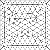
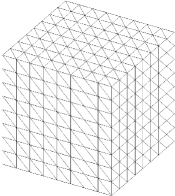
Figure 1. The triangular mesh (left) and tetrahedral mesh (right).

Example 1. In the first example, we solve a biharmonic equation in two dimensions defined on the squared domain $\Omega=(0,1)^{2}$. The exact solution is given by

$$u(x,y)=\sin^{2}(\pi x)\sin^{2}(\pi y).$$

We apply the approximation space $U_{h}^{m}$ of the accuracy $m=2,3,4$ to solve the biharmonic problem on the triangular meshes with the mesh size $h=1/10,1/20,1/40,1/80$. We first test the accuracy of the scheme. The numerical errors under both the energy norm and the $L^{2}$ norm are plotted in Fig. 2. It can be seen that the numerically detected convergence rates validate the theoretical preconditions in Theorem 20.

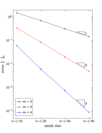
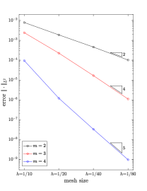
Figure 2. The numerical errors under the energy norm (left)/$L^{2}$ norm (right) in Example 1.

We also numerically compare the proposed method with the interior penalty discontinuous Galerkin method and the $C^{0}$ interior penalty method. In Fig. 3, we plot the $L^{2}$ errors of solutions from different methods against the number of degrees of freedom. It can be seen that all methods have same convergence rates, which are consistent with the error estimates. To achieve the same $L^{2}$ error, the reconstructed method uses less degrees of freedom and is observed to be more computationally efficient than other methods.

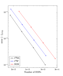
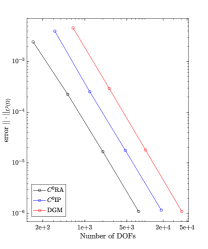
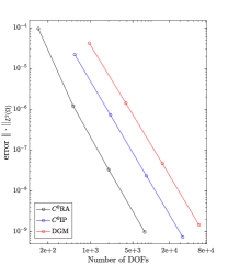
Figure 3. The numerical comparison of $L^{2}$ errors for different methods (from left to right, $m=2,3,4$).

We further present the numerical performance of the preconditioning method in solving the resulting linear system. The condition numbers of the system $A_{m}$ and the preconditioned system $A_{\mathcal{L}}^{-1}A_{m}$ are listed in Tab. 1. It is clear that $\kappa(A_{m})$ grows very fast at the speed of $O(h^{-4})$ while for all $m$, $\kappa(A_{\mathcal{L}}^{-1}A_{m})$ increases very slightly as the mesh size tends to zero. The numerical observation illustrates the results given in Theorem 29. As stated in the previous section, we apply the preconditioned CG method using the approximation of $A_{\mathcal{L}}^{-1}$ as the preconditioner, i.e. Algorithm 2 and Algorithm 3, for the resulting linear system. The stopping criteria is set by $\|\boldsymbol{\mathrm{r}}_{k}\|_{l^{2}}\leq 10^{-9}\|\boldsymbol{\mathrm{b}}\|_{l^{2}}$, where $\boldsymbol{\mathrm{r}}_{k}:=\boldsymbol{\mathrm{b}}-A_{m}\boldsymbol{x}_{k}$ is the residual at step $k$. The iteration counts for PCG/CG methods are gathered in Tab. 2. For the standard CG method, the iteration count quadruples after the mesh is refined, which agrees with the estimation to the condition number. For the preconditioning methods, the required steps are numerically observed to grow slightly when the mesh size approaches zero. The numerical results illustrate the efficiency of our method.

		1/10	1/20	1/40	1/80
2	$\kappa(A_{\mathcal{L}}^{-1}A_{m})$	10.07	15.00	16.12	17.23
	$\kappa(A_{m})$	3.673e+3	9.217e+4	1.530e+6	2.735e+7
3	$\kappa(A_{\mathcal{L}}^{-1}A_{m})$	16.69	21.15	23.09	25.02
	$\kappa(A_{m})$	6.672e+3	1.256e+5	2.353e+6	4.173e+7
4	$\kappa(A_{\mathcal{L}}^{-1}A_{m})$	32.75	49.83	60.37	65.45
	$\kappa(A_{m})$	1.582e+4	2.662e+5	4.26e+6	7.172e+7

Table 1. The condition numbers in Example 1.

$m$		1/10	1/20	1/40	1/80
2	Algorithm 2 for $A_{\mathcal{L}}^{-1}$	21	28	29	30
	Algorithm 3 for $A_{\mathcal{L}}^{-1}$	21	27	29	31
	Identity	109	538	2338	$>3000$
3	Algorithm 2 for $A_{\mathcal{L}}^{-1}$	31	45	51	54
	Algorithm 3 for $A_{\mathcal{L}}^{-1}$	31	46	49	51
	Identity	109	649	$>3000$	$>3000$
4	Algorithm 2 for $A_{\mathcal{L}}^{-1}$	46	58	71	73
	Algorithm 3 for $A_{\mathcal{L}}^{-1}$	46	62	67	71
	Identity	118	847	$>3000$	$>3000$

Table 2. The convergence steps for PCG/CG methods in Example 1.

Example 2. In this example, we solve a three-dimensional problem in the cubic domain $\Omega=(0,1)^{3}$. The analytic solution is chosen to be

$$u(x,y,z)=\sin(\pi x)\sin(\pi y)\sin(\pi z).$$

The source function and boundary conditions are taken accordingly. This problem is discretized on a series of tetrahedral meshes with the mesh size $h=1/8,1/16,1/32,1/64$. The numerical errors under $L^{2}$ norm and the energy norm are are shown in Fig. 4. As predicted, the numerically detected errors decrease sharply for the proposed scheme, which agree with the theoretical estimation.

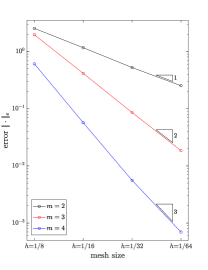
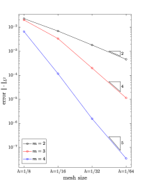
Figure 4. The numerical errors under the energy norm (left)/$L^{2}$ norm (right) in Example 2.

For the linear systems $A_{m}$ and $A_{\mathcal{L}}^{-1}A_{m}$, their condition numbers are collected in Tab. 3. Similar to the case of two dimensions, it can be seen that $\kappa(A_{m})$ grows at the rate $O(h^{-4})$ while $\kappa(A_{\mathcal{L}}^{-1}A_{m})$ is nearly constant. The convergence steps of linear solvers are gathered in Tab. 4. In three dimensions, the linear solver can be significantly accelerated with both multigrid methods for $A_{\mathcal{L}}^{-1}$. The numerical results again illustrate the efficiency of the preconditioning method.

		1/8	1/16	1/32	1/64
2	$\kappa(A_{\mathcal{L}}^{-1}A_{m})$	6.64	13.26	17.89	18.47
	$\kappa(A_{m})$	1.013e+2	1.152e+3	1.957e+4	3.703e+5
3	$\kappa(A_{\mathcal{L}}^{-1}A_{m})$	9.94	26.29	38.10	42.03
	$\kappa(A_{m})$	2.286e+2	5.012e+3	1.106e+5	1.95e+6
4	$\kappa(A_{\mathcal{L}}^{-1}A_{m})$	40.50	158.47	219.59	227.29
	$\kappa(A_{m})$	5.164e+2	3.652e+4	6.292e+5	1.136e+7

Table 3. The condition numbers in Example 2.

$m$		1/8	1/16	1/32	1/64
2	Algorithm 2 for $A_{\mathcal{L}}^{-1}$	25	38	48	52
	Algorithm 3 for $A_{\mathcal{L}}^{-1}$	25	37	47	49
	Identity	99	366	1391	$>3000$
3	Algorithm 2 for $A_{\mathcal{L}}^{-1}$	29	50	63	69
	Algorithm 3 for $A_{\mathcal{L}}^{-1}$	28	49	65	71
	Identity	189	996	$>3000$	$>3000$
4	Algorithm 2 for $A_{\mathcal{L}}^{-1}$	53	106	139	143
	Algorithm 3 for $A_{\mathcal{L}}^{-1}$	53	108	137	141
	Identity	213	1094	$>3000$	$>3000$

Table 4. The convergence steps for PCG/CG methods in Example 2.

Appendix A

In this appendix, we present the method for computing the constant $\Lambda_{m}$ and $\Lambda_{m,K}$ on each element after constructing element patches for a given mesh $\mathcal{T}_{h}$. For every $K\in\mathcal{T}_{h}$, we let $p_{1},p_{2},\ldots,p_{l}$ be a group of standard orthogonal basis functions in $\mathcal{P}_{m}(K)$ under the $L^{2}$ inner product $(\cdot,\cdot)_{L^{2}(K)}$. Then, any $q\in\mathcal{P}_{m}(K)$ can be expressed by a group coefficients $\boldsymbol{\alpha}=\{a_{j}\}_{j=1}^{l}\in\mathbb{R}^{l}$ such that $q=\sum_{j=1}^{l}a_{j}p_{j}$. In addition, $q$ and all $p_{j}$ can be naturally extended to the domain $\mathcal{D}(K)$. The main step to obtain $\Lambda_{m}$ is to compute $\Lambda_{m,K}$ per element. By $\{p_{j}\}_{j=1}^{l}$, $\Lambda_{m,K}$ can be written into an algebraic form as

$$\Lambda_{m,K}^{2}=\max_{\boldsymbol{\alpha}\in\mathbb{R}^{l}}\frac{|\boldsymbol{\alpha}|_{l^{2}}^{2}}{h_{K}^{d}\boldsymbol{\alpha}^{T}B_{K}\boldsymbol{\alpha}},\quad B_{K}=\{b_{ij}\}_{l\times l},\quad b_{ij}=\sum_{\boldsymbol{x}\in\mathcal{I}(K)}p_{i}(\boldsymbol{x})p_{j}(\boldsymbol{x}).$$

From the above matrix representation, we have that $\Lambda_{m,K}=(h_{K}^{d}\sigma_{\min}(B_{K}))^{-1/2}$, where $\sigma_{\min}(B_{K})$ is the smallest singular value to the matrix $B_{K}$. Therefore, it is enough to observe all the smallest singular values $\sigma_{\min}(B_{K})$, and $\Lambda_{m}$ can be further obtained by (8).

In Fig. 5, we plot the constant $\Lambda_{m}$ against the threshold $N_{m}$ on the triangular mesh with the mesh size $h=1/40$. It is evident that the constant $\Lambda_{m}$ is nearly a constant and increases very slightly when selecting a large threshold $N_{m}$. This numerical observation illustrates the statement given in Remark 1 that $\Lambda_{m}$ will admit a uniform upper bound for large $N_{m}$. Roughly speaking, $N_{m}$ is close to $1.5\mathrm{dim}(\mathcal{P}_{m}(\cdot))$. In the computer implementation, the constant $\Lambda_{m}$ can also serve as an indicator to show whether the element patch is proper. After constructing all element patches, we compute the value of $\Lambda_{m}$. If $\Lambda_{m}\rightarrow\infty$, we can increase the value of $N_{m}$ until $\Lambda_{m}\leq 10\min_{K\in\mathcal{T}_{h}}\Lambda_{m,K}$.

In Fig. 6, we plot the constant $\Lambda_{m}$ in three dimensions on the tetrahedral mesh with the mesh size $h=1/32$. The numerical result is similar to the case of two dimensions. We still find that $\Lambda_{m}$ is close to a constant for a large $N_{m}$.

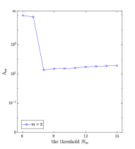
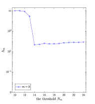
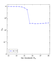
Figure 5. The constant $\Lambda_{m}$ in two dimensions.

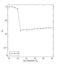
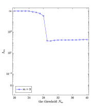
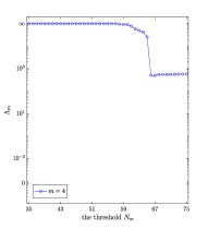
Figure 6. The constant $\Lambda_{m}$ in three dimensions.

Appendix B

In this appendix, we verify the estimate (16) in both two and three dimensions. Let $W_{h}^{m}:=\{w_{h}\in L^{2}(\Omega):\ w_{h}|_{K}\in\mathcal{P}_{m}(K),\ \forall K\in\mathcal{T}_{h}\}$ be the discontinuous finite element spaces of degree $m$. Let $\boldsymbol{\mathrm{W}}_{h}^{m}:=(W_{h}^{m})^{d}$, $\boldsymbol{\mathrm{Q}}_{h}^{m}:=\boldsymbol{\mathrm{W}}_{h}^{m}\cap(H^{1}(\Omega))^{d}$ be the vector-valued discontinuous/$C^{0}$ finite element spaces. The estimate (16) is based on the following discrete Maxwell inequality.

Lemma 12.

There exists a constant $C$ such that

(42) $$\|\nabla\boldsymbol{q}_{h}\|_{L^{2}(\Omega)}^{2}\leq\|\nabla\cdot\boldsymbol{q}_{h}\|_{L^{2}(\Omega)}^{2}+\|\nabla\times\boldsymbol{q}_{h}\|_{L^{2}(\Omega)}^{2}+C\sum_{e\in\mathcal{E}_{h}^{b}}h_{e}^{-1}\|\boldsymbol{\mathrm{n}}\times\boldsymbol{q}_{h}\|_{L^{2}(e)}^{2},\quad\forall\boldsymbol{q}_{h}\in\boldsymbol{\mathrm{Q}}_{h}^{m}.$$

Proof.

Since $\Omega$ is convex, we first recall the Maxwell inequality [21], which reads

(43) $$\|\nabla{\boldsymbol{w}}\|_{L^{2}(\Omega)}\leq\|\nabla\cdot{\boldsymbol{w}}\|_{L^{2}(\Omega)}+\|\nabla\times{\boldsymbol{w}}\|_{L^{2}(\Omega)},$$

for any $\boldsymbol{w}\in(H^{1}(\Omega))^{d}$ with $\boldsymbol{\mathrm{n}}\times\boldsymbol{w}=\boldsymbol{0}$ on the boundary $\partial\Omega$. It is noted that $\boldsymbol{q}_{h}\in(H^{1}(\Omega))^{d}$ but its tangential trace does not vanish on $\partial\Omega$. We are aiming to construct an auxiliary function $\boldsymbol{w}_{h}$ with zero tangential trace on $\partial\Omega$ from $\boldsymbol{q}_{h}$. Let $\mathcal{M}:=\{\boldsymbol{\nu}_{0},\boldsymbol{\nu}_{1},\ldots,\boldsymbol{\nu}_{n}\}$ denote the Lagrange nodes for the space $\boldsymbol{\mathrm{Q}}_{h}^{m}$, and we let $\{\phi_{\boldsymbol{\nu}_{0}},\phi_{\boldsymbol{\nu}_{1}},\ldots,\phi_{\boldsymbol{\nu}_{n}}\}$ be the corresponding basis functions such that $\phi_{\boldsymbol{\nu}_{i}}(\boldsymbol{\nu}_{j})=\delta_{ij}$. We let $\boldsymbol{q}_{h}=(q_{h}^{1},\ldots,q_{h}^{d})^{T}$ be expanded by the coefficients $\{\alpha_{\boldsymbol{\nu}}^{i}\}_{\boldsymbol{\nu}\in\mathcal{M},1\leq i\leq d}$ such that

$$\boldsymbol{q}_{h}=\begin{bmatrix}q_{h}^{1}\\ \ldots\\ q_{h}^{d}\end{bmatrix}=\begin{bmatrix}\sum_{\boldsymbol{\nu}\in\mathcal{M}}\alpha_{\boldsymbol{\nu}}^{1}\phi_{\boldsymbol{\nu}}\\ \ldots\\ \sum_{\boldsymbol{\nu}\in\mathcal{M}}\alpha_{\boldsymbol{\nu}}^{d}\phi_{\boldsymbol{\nu}}\end{bmatrix}=\sum_{\boldsymbol{\nu}\in\mathcal{M}}\boldsymbol{\alpha}_{\boldsymbol{\nu}}\phi_{\boldsymbol{\nu}},\quad\boldsymbol{\alpha}_{\boldsymbol{\nu}}=(\alpha_{\boldsymbol{\nu}}^{1},\ldots,\alpha_{\boldsymbol{\nu}}^{d})^{T}.$$

The set $\mathcal{M}$ is further divided into three subsets:

(44) $$\mathcal{M}_{i} :=\left\{\boldsymbol{\nu}\in\mathcal{M}:\ \boldsymbol{\nu}\text{ is interior to the domain }\Omega\right\},$$

$$\mathcal{M}_{v} :=\left\{\begin{aligned} &\left\{\boldsymbol{\nu}\in\mathcal{M}:\ \boldsymbol{\nu}\text{ is a vertex of the polygonal boundary }\partial\Omega\right\},&&d=2,\\ &\left\{\boldsymbol{\nu}\in\mathcal{M}:\ \boldsymbol{\nu}\text{ lies on an edge of the polyhedral boundary }\partial\Omega\right\},&&d=3,\\ \end{aligned}\right.$$

$$\mathcal{M}_{b} :=\mathcal{M}\backslash(\mathcal{M}_{i}\cup\mathcal{M}_{v}).$$

For any $\boldsymbol{\nu}\in\mathcal{M}_{b}$, there exists a face $e_{\boldsymbol{\nu}}\in\mathcal{E}_{h}^{b}$ such that $\boldsymbol{\nu}\in\overline{e_{\boldsymbol{\nu}}}$. For any $\boldsymbol{\nu}\in\mathcal{M}_{v}$, there exist two nonparallel faces $e_{\boldsymbol{\nu}}^{1},e_{\boldsymbol{\nu}}^{2}\in\mathcal{E}_{h}^{b}$ such that $\boldsymbol{\nu}\in\overline{e_{\boldsymbol{\nu}}^{1}}\cap\overline{e_{\boldsymbol{\nu}}^{2}}$.

We next construct a group of new coefficients $\{\beta_{\boldsymbol{\nu}}^{i}\}_{\boldsymbol{\nu}\in\mathcal{M},1\leq i\leq d}$ by

(45) $$\beta_{\boldsymbol{\nu}}^{i}=\begin{cases}\alpha_{\boldsymbol{\nu}}^{i},&\boldsymbol{\nu}\in\mathcal{M}_{i},\\ \widetilde{\beta}_{\boldsymbol{\nu}}^{i},&\boldsymbol{\nu}\in\mathcal{M}_{b},\\ 0,&\boldsymbol{\nu}\in\mathcal{M}_{v},\\ \end{cases}\quad 1\leq i\leq d,\quad\boldsymbol{\beta}_{\boldsymbol{\nu}}=(\beta_{\boldsymbol{\nu}}^{1},\ldots\beta_{\boldsymbol{\nu}}^{d})^{T}.$$

For any $\boldsymbol{\nu}\in\mathcal{M}_{b}$, $\widetilde{\beta}_{\boldsymbol{\nu}}^{i}$ is determined by the equation

(46) $$\boldsymbol{\mathrm{n}}\times{\boldsymbol{\beta}}_{\boldsymbol{\nu}}=\boldsymbol{0},\quad\boldsymbol{\mathrm{n}}\cdot{\boldsymbol{\beta}}_{\boldsymbol{\nu}}=\boldsymbol{\mathrm{n}}\cdot\boldsymbol{\alpha}_{\boldsymbol{\nu}},$$

where $\boldsymbol{\mathrm{n}}$ is the unit outward normal vector on $e_{\boldsymbol{\nu}}$. The new polynomial $\boldsymbol{w}_{h}\in\boldsymbol{\mathrm{Q}}_{h}^{m}$ is constructed by $\{\beta_{\boldsymbol{\nu}}^{i}\}_{\boldsymbol{\nu}\in\mathcal{M},1\leq i\leq d}$ that

$$\boldsymbol{w}_{h}=\begin{bmatrix}w_{h}^{1}\\ \ldots\\ w_{h}^{d}\end{bmatrix}=\begin{bmatrix}\sum_{\boldsymbol{\nu}\in\mathcal{M}}\beta_{\boldsymbol{\nu}}^{1}\phi_{\boldsymbol{\nu}}\\ \ldots\\ \sum_{\boldsymbol{\nu}\in\mathcal{M}}\beta_{\boldsymbol{\nu}}^{d}\phi_{\boldsymbol{\nu}}\end{bmatrix}=\sum_{\boldsymbol{\nu}\in\mathcal{M}}\boldsymbol{\beta}_{\boldsymbol{\nu}}\phi_{\boldsymbol{\nu}}.$$

By (44), we have that

$$\|\nabla(\boldsymbol{q}_{h}-{\boldsymbol{w}}_{h})\|_{L^{2}(\Omega)}^{2}\leq C\sum_{\nu\in\mathcal{M}_{b}\cup\mathcal{M}_{v}}\|\nabla\phi_{\boldsymbol{\nu}}\|_{L^{2}(\Omega)}^{2}|\boldsymbol{\alpha}_{\boldsymbol{\nu}}-\boldsymbol{\beta}_{\boldsymbol{\nu}}|^{2}.$$

From the scaling argument [26], we know that $\|\nabla\phi_{\boldsymbol{\nu}}\|_{L^{2}(\Omega)}^{2}\leq Ch_{e_{\boldsymbol{\nu}}}^{d-2}$ for $\forall\boldsymbol{\nu}\in\mathcal{M}_{b}$. We deduce that

$$\sum_{\boldsymbol{\nu}\in\mathcal{M}_{b}}\|\nabla \phi_{\boldsymbol{\nu}}\|_{L^{2}(\Omega)}^{2}|\boldsymbol{\alpha}_{\boldsymbol{\nu}}-\boldsymbol{\beta}_{\boldsymbol{\nu}}|^{2}\leq C\sum_{\boldsymbol{\nu}\in\mathcal{M}_{b}}h_{e_{\boldsymbol{\nu}}}^{d-2}\left(|\boldsymbol{\mathrm{n}}\times(\boldsymbol{\alpha}_{\boldsymbol{\nu}}-\boldsymbol{\beta}_{\boldsymbol{\nu}})|^{2}+|\boldsymbol{\mathrm{n}}\cdot(\boldsymbol{\alpha}_{\boldsymbol{\nu}}-\boldsymbol{\beta}_{\boldsymbol{\nu}})|^{2}\right)$$

$$=C\sum_{\boldsymbol{\nu}\in\mathcal{M}_{b}}h_{e_{\boldsymbol{\nu}}}^{d-2}|\boldsymbol{\mathrm{n}}\times\boldsymbol{\alpha}_{\boldsymbol{\nu}}|^{2}=C\sum_{\boldsymbol{\nu}\in\mathcal{M}_{b}}h_{e_{\boldsymbol{\nu}}}^{d-2}|\boldsymbol{\mathrm{n}}\times\boldsymbol{q}_{h}(\boldsymbol{\nu})|^{2}$$

$$\leq C\sum_{\boldsymbol{\nu}\in\mathcal{M}_{b}}h_{e_{\boldsymbol{\nu}}}^{d-2}\|\boldsymbol{\mathrm{n}}\times\boldsymbol{q}_{h}\|_{L^{\infty}(e_{\boldsymbol{\nu}})}^{2}\leq C\sum_{\boldsymbol{\nu}\in\mathcal{M}_{b}}h_{e_{\boldsymbol{\nu}}}^{-1}\|\boldsymbol{\mathrm{n}}\times\boldsymbol{q}_{h}\|_{L^{2}(e_{\boldsymbol{\nu}})}^{2}\leq C\sum_{e\in\mathcal{E}_{h}^{b}}h_{e}^{-1}\|\boldsymbol{\mathrm{n}}\times\boldsymbol{q}_{h}\|_{L^{2}(e)}^{2}.$$

For any $\boldsymbol{\nu}\in\mathcal{M}_{v}$, we let $\boldsymbol{\mathrm{n}}_{1},\boldsymbol{\mathrm{n}}_{2}$ be the unit outward normal vectors on $e_{\boldsymbol{\nu}}^{1},e_{\boldsymbol{\nu}}^{2}$, respectively. Since $\boldsymbol{\mathrm{n}}_{1}$ and $\boldsymbol{\mathrm{n}}_{2}$ are not parallel, by the norm equivalence over finite dimensional spaces, there exists a constant $C$ only depends on $\Omega$ such that

$$|\boldsymbol{v}|^{2}\leq C(|\boldsymbol{\mathrm{n}}_{1}\times\boldsymbol{v}|^{2}+|\boldsymbol{\mathrm{n}}_{2}\times\boldsymbol{v}|^{2}),\quad\forall\boldsymbol{v}\in\mathbb{R}^{d}.$$

We derive that

$$\sum_{\boldsymbol{\nu}\in\mathcal{M}_{v}} \|\nabla\phi_{\boldsymbol{\nu}}\|_{L^{2}(\Omega)}^{2}|\boldsymbol{\alpha}_{\boldsymbol{\nu}}-\boldsymbol{\beta}_{\boldsymbol{\nu}}|^{2}=\sum_{\boldsymbol{\nu}\in\mathcal{M}_{v}}\|\nabla\phi_{\boldsymbol{\nu}}\|_{L^{2}(\Omega)}^{2}|\boldsymbol{\alpha}_{\boldsymbol{\nu}}|^{2}\leq C\sum_{\boldsymbol{\nu}\in\mathcal{M}_{v}}\|\nabla\phi_{\boldsymbol{\nu}}\|_{L^{2}(\Omega)}^{2}\left(|\boldsymbol{\mathrm{n}}_{1}\times\boldsymbol{\alpha}_{\boldsymbol{\nu}}|^{2}+|\boldsymbol{\mathrm{n}}_{2}\times\boldsymbol{\alpha}_{\boldsymbol{\nu}}|^{2}\right)$$

$$\leq C\sum_{\boldsymbol{\nu}\in\mathcal{M}_{v}}\left(h_{e_{\boldsymbol{\nu}}^{1}}^{d-2}|\boldsymbol{\mathrm{n}}_{1}\times\boldsymbol{\alpha}_{\boldsymbol{\nu}}|^{2}+h_{e_{\boldsymbol{\nu}}^{2}}^{d-2}|\boldsymbol{\mathrm{n}}_{2}\times\boldsymbol{\alpha}_{\boldsymbol{\nu}}|^{2}\right)\leq C\sum_{\boldsymbol{\nu}\in\mathcal{M}_{v}}\left(h_{e_{\boldsymbol{\nu}}^{1}}^{d-2}|\boldsymbol{\mathrm{n}}_{1}\times\boldsymbol{q}_{h}(\boldsymbol{\nu})|^{2}+h_{e_{\boldsymbol{\nu}}^{2}}^{d-2}|\boldsymbol{\mathrm{n}}_{2}\times\boldsymbol{q}_{h}(\boldsymbol{\nu})|^{2}\right)$$

$$\leq C\sum_{\boldsymbol{\nu}\in\mathcal{M}_{v}}\left(h_{e_{\boldsymbol{\nu}}^{1}}^{-1}\|\boldsymbol{\mathrm{n}}_{1}\times\boldsymbol{q}_{h}\|_{L^{2}(e_{\boldsymbol{\nu}}^{1})}^{2}+h_{e_{\boldsymbol{\nu}}^{2}}^{-1}\|\boldsymbol{\mathrm{n}}_{2}\times\boldsymbol{q}_{h}\|_{L^{2}(e_{\boldsymbol{\nu}}^{2})}^{2}\right)\leq C\sum_{e\in\mathcal{E}_{h}^{b}}h_{e}^{-1}\|\boldsymbol{\mathrm{n}}\times\boldsymbol{q}_{h}\|_{L^{2}(e)}^{2}.$$

Finally, we arrive at

(47) $$\|\nabla(\boldsymbol{q}_{h}-\boldsymbol{w}_{h})\|_{L^{2}(\Omega)}^{2}\leq C\sum_{e\in\mathcal{E}_{h}^{b}}h_{e}^{-1}\|\boldsymbol{\mathrm{n}}\times\boldsymbol{q}_{h}\|_{L^{2}(e)}^{2},$$

Clearly, $\boldsymbol{w}_{h}$ satisfies the estimate (43). Together with (47), we have that

$$\|\nabla\boldsymbol{q}_{h}\|_{L^{2}(\Omega)} \leq\|\nabla\boldsymbol{w}_{h}\|_{L^{2}(\Omega)}+\|\nabla(\boldsymbol{q}_{h}-\boldsymbol{w}_{h})\|_{L^{2}(\Omega)}$$

$$\leq\|\nabla\cdot{\boldsymbol{w}}_{h}\|_{L^{2}(\Omega)}+\|\nabla\times{\boldsymbol{w}}_{h}\|_{L^{2}(\Omega)}+\|\nabla(\boldsymbol{q}_{h}-\boldsymbol{w}_{h})\|_{L^{2}(\Omega)}$$

$$\leq\|\nabla\cdot\boldsymbol{q}_{h}\|_{L^{2}(\Omega)}+\|\nabla\times\boldsymbol{q}_{h}\|_{L^{2}(\Omega)}+C\|\nabla(\boldsymbol{q}_{h}-\boldsymbol{w}_{h})\|_{L^{2}(\Omega)},$$

which indicates the estimate (42). This completes the proof. ∎

The estimate (42) can be extended to the discontinuous space $\boldsymbol{\mathrm{W}}_{h}^{m}$, which reads

(48) $$\sum_{K\in\mathcal{T}_{h}}\|\nabla\boldsymbol{w}_{h}\|_{L^{2}(K)}^{2} \leq\sum_{K\in\mathcal{T}_{h}}(\|\nabla\cdot\boldsymbol{w}_{h}\|_{L^{2}(K)}^{2}+\|\nabla\times\boldsymbol{w}_{h}\|_{L^{2}(K)}^{2})$$

$$+ C\sum_{e\in\mathcal{E}_{h}^{i}}h_{e}^{-1}\|[[\boldsymbol{w}_{h}]]\|_{L^{2}(e)}^{2}+C\sum_{e\in\mathcal{E}_{h}^{b}}h_{e}^{-1}\|\boldsymbol{\mathrm{n}}\times\boldsymbol{w}_{h}\|_{L^{2}(e)}^{2},\quad\forall\boldsymbol{w}_{h}\in\boldsymbol{\mathrm{W}}_{h}^{m},$$

by applying the Oswald interpolant. From [26, Theorem 2.1], for any $\boldsymbol{w}_{h}\in\boldsymbol{\mathrm{W}}_{h}^{m}$, there exists $\boldsymbol{q}_{h}\in\boldsymbol{\mathrm{Q}}_{h}^{m}$ such that

(49) $$\sum_{K\in\mathcal{T}_{h}}(h_{K}^{2}\|\boldsymbol{w}_{h}-\boldsymbol{q}_{h}\|_{L^{2}(K)}^{2}+\|\boldsymbol{w}_{h}-\boldsymbol{q}_{h}\|_{H^{1}(K)}^{2})\leq C\sum_{e\in\mathcal{E}_{h}^{i}}h_{e}^{-1}\|[[\boldsymbol{w}_{h}]]\|_{L^{2}(e)}^{2}.$$

Then, the estimate (48) can be easily verified using estimates (49) and (42) and the trace estimate.

Finally, let us present the main conclusion in this appendix.

Lemma 13.

There exists a constant $C$ such that

(50) $$\sum_{K\in\mathcal{T}_{h}}\|D^{2}v_{h}\|_{L^{2}(K)}^{2} \leq\sum_{K\in\mathcal{T}_{h}}\|\Delta v_{h}\|_{L^{2}(K)}^{2}+C(\sum_{e\in\mathcal{E}_{h}^{i}}h_{e}^{-1}\|[[\nabla_{\boldsymbol{\mathrm{n}}}v_{h}]]\|_{L^{2}(e)}^{2}+\sum_{e\in\mathcal{E}_{h}}h_{e}^{-3}\|[[v_{h}]]\|_{L^{2}(e)}^{2}),$$

for $\forall v_{h}\in W_{h}^{m}$.

Proof.

Let $\boldsymbol{q}_{h}\in\boldsymbol{\mathrm{W}}_{h}^{m}$ be determined by $\boldsymbol{q}_{h}|_{K}=\nabla v_{h}|_{K}$ for $\forall K\in\mathcal{T}_{h}$. Then, it is clear that $\nabla\times\boldsymbol{q}_{h}|_{K}=0$ on every $K\in\mathcal{T}_{h}$. For any interior face $e\in\mathcal{E}_{h}^{i}$, we apply the inverse estimate to find that

$$h_{e}^{-1}\|[[\boldsymbol{q}_{h}]]\|_{L^{2}(e)}^{2} \leq h_{e}^{-1}(\|[[\boldsymbol{\mathrm{n}}\times\boldsymbol{q}_{h}]]\|_{L^{2}(e)}^{2}+\|[[\boldsymbol{\mathrm{n}}\cdot\boldsymbol{q}_{h}]]\|_{L^{2}(e)}^{2})=h_{e}^{-1}(\|[[\boldsymbol{\mathrm{n}}\times\nabla v_{h}]]\|_{L^{2}(e)}^{2}+\|[[\nabla_{\boldsymbol{\mathrm{n}}}v_{h}]]\|_{L^{2}(e)}^{2})$$

$$\leq C(h_{e}^{-3}\|[[v_{h}]]\|_{L^{2}(e)}^{2}+h_{e}^{-1}\|[[\nabla_{\boldsymbol{\mathrm{n}}}v_{h}]]\|_{L^{2}(e)}^{2}).$$

From the estimate (48), we have that

$$\sum_{K\in\mathcal{T}_{h}} \|D^{2}v_{h}\|_{L^{2}(K)}^{2}=\sum_{K\in\mathcal{T}_{h}}\|\nabla\boldsymbol{q}_{h}\|_{L^{2}(K)}^{2}$$

$$\leq\sum_{K\in\mathcal{T}_{h}}\|\nabla\cdot\boldsymbol{q}_{h}\|_{L^{2}(K)}^{2}+C\sum_{e\in\mathcal{E}_{h}^{i}}h_{e}^{-1}\|[[\boldsymbol{q}_{h}]]\|_{L^{2}(e)}^{2}+C\sum_{e\in\mathcal{E}_{h}^{b}}h_{e}^{-1}\|\boldsymbol{\mathrm{n}}\times\boldsymbol{q}_{h}\|_{L^{2}(e)}^{2}$$

$$\leq\sum_{K\in\mathcal{T}_{h}}\|\Delta v_{h}\|_{L^{2}(K)}^{2}+C\sum_{e\in\mathcal{E}_{h}^{i}}h_{e}^{-1}\|[[\nabla v_{h}]]\|_{L^{2}(e)}^{2}+C\sum_{e\in\mathcal{E}_{h}}h_{e}^{-3}\|[[v_{h}]]\|_{L^{2}(e)}^{2},$$

which completes the proof. ∎