Semi and fully-discrete analysis of lowest-order nonstandard finite element methods for the biharmonic wave problem

Abstract

This paper discusses lowest-order nonstandard finite element methods for space discretization and explicit and implicit schemes for time discretization of the biharmonic wave equation with clamped boundary conditions. A modified Ritz projection operator defined on $H^{2}_{0}(\Omega)$ ensures error estimates under appropriate regularity assumptions on the solution. Stability results and error estimates of optimal order are established in suitable norms for the semidiscrete and explicit/implicit fully-discrete versions of the proposed schemes. Finally, we report on numerical experiments using explicit and implicit schemes for time discretization and Morley, discontinuous Galerkin, and C⁰ interior penalty schemes for space discretization, that validate the theoretical error estimates.

Key words. Biharmonic wave equation, modified Ritz projection, stability, error estimates.

1 Introduction

1.1 Scope and problem formulation

The biharmonic wave model finds application in representing various physical phenomena, such as the bending of plates, and elasticity in thin plates under dynamic loading conditions. This is also a foundational part for more advanced linear and nonlinear models such as Kirchhoff-type equations using Monge–Ampère forms [16, 20, 37], which in turn serve as model for the transmission of waves, damping phenomena, standing waves, properties of ferromagnetic materials, and vibration modes within plates.

This paper analyses lowest-order nonstandard finite element methods (FEMs) for space discretization and semidiscrete and explicit and implicit time discretization schemes for the biharmonic wave equation

$$u_{tt}+\Delta^{2}u=f(x,t),\quad(x,t)\in\Omega\times\left(0,T\right],$$ (1.1)

with initial and clamped boundary conditions

$$u(x,0)=u^{0}(x),\quad u_{t}(x,0)=v^{0}(x)\text{ in }\Omega;\quad u=\frac{\partial u}{\partial n}=0\text{ on }\partial\Omega\times\left(0,T\right].$$ (1.2)

Here $\Omega$ is a bounded polygonal Lipschitz domain in $\mathbb{R}^{2}$ with boundary $\partial\Omega$ and outward-pointing unit normal $n$, $\Delta^{2}u:=\frac{\partial^{4}u}{\partial x^{4}}+2\>\frac{\partial^{4}u}{\partial x^{2}\partial y^{2}}+\frac{\partial^{4}u}{\partial y^{4}}$ denotes the biharmonic operator, $\partial u/\partial n=\nabla u\cdot n$ is the outer normal derivative of $u$ on $\partial\Omega$, $u_{t}$, $u_{tt}$ denote the first- and second-order derivatives with respect to time, respectively, and $f\in L^{2}(L^{2}(\Omega))$ is a given source function.

1.2 Literature overview

Despite being a classical problem, research on the biharmonic problem remains an area of active interest, as evidenced by recent contributions [6, 11, 21, 31, 39, 45]. Constructing $C^{1}$ finite elements, which ensure continuity of both basis functions and their first-order derivatives over the closure of the domain and conform to the space $H^{2}(\Omega)$, for fourth-order problems is notoriously challenging. Consequently, nonstandard FEMs such as the Morley FEM [10, 40, 44], discontinuous Galerkin (dG) FEM [25, 24], and the $C^{0}$ interior penalty ($C^{0}$IP) method [35, 43] present attractive alternatives. Recently, an abstract framework for analyzing lowest-order FEMs for the clamped plate biharmonic problem has been established in [11]. One aim of this paper is to investigate and adapt such an analysis for the case of biharmonic wave problems.

Fourth-order parabolic problems have been addressed using the Morley FEM [18], dG FEM [26], and the $C^{0}$ interior penalty method [30], typically employing the backward Euler method for time discretization. Similar numerical methods have been extensively studied for second-order hyperbolic equations, as seen in [15, 28, 27, 8, 19, 36, 22, 42]. However, despite their importance in applications, the literature on the numerical approximation of the fourth-order biharmonic wave equation is relatively sparse. Notable contributions include [3], where the biharmonic wave problem is discretized using classical $C^{1}$-conforming Bogner–Fox–Schmit elements in space, combined with Galerkin and collocation techniques for time discretization. A mixed velocity-moment formulation is analyzed in [4] for the fourth-order Kirchhoff–Love dynamic plate equations using Lagrange FEs in space with both explicit and implicit central difference schemes in time. Additionally, error estimates for the fourth-order wave equation have been derived using a combination of discrete Galerkin and second-order accurate methods for space and time discretizations [23]. Mixed FEMs for fourth-order wave equations with various boundary conditions and optimal error estimates have been studied in [33, 32].

1.3 Specific contributions

We now describe the main contributions of this paper. Firstly, to the best of our knowledge, this is the first attempt to analyse biharmonic wave equation using nonstandard FEMs with a unified approach. The Courant–Friedrichs–Lewy (CFL) condition for the wave equation is extensively discussed in the literature (see, e.g., [29]), but its analysis specifically targeted for the biharmonic wave equation was still missing. Secondly, the regularity results advanced in this work (see Lemma 1.1) are established under (a) certain smoothness assumptions on $f$ and its derivatives and (b) for non-homogeneous initial conditions, which are different from those in [41, Theorem 7.1]. This is attained by using the approach of explicit solution representation for proving the regularity results rather than using the energy arguments as discussed in [41]. Thirdly, we employ a modified Ritz projection (see the definition of $\mathcal{R}_{h}$ in (2.8)) on $H^{2}_{0}(\Omega)$, which is defined with the help of the companion operator (cf. [11]). It is also important to note that this modified Ritz projection readily yields $L^{2}-$estimates (see Corollary 3.8, Remark 4.4 for the fully discrete schemes) based on the energy norm error estimate of the solution and $L^{2}-$error estimate of time derivative of the solution without the need for any additional analysis.

Note also that the test function in the continuous weak form is selected following an approach that consists in lifting discrete functions to $H^{2}_{0}(\Omega)$ using a suitably defined smoother. This novel technique helps to bound the semidiscrete and fully-discrete errors by manipulating the continuous and discrete formulations. This represents an improvement with respect to more standard approaches that assume higher regularity of the continuous solution and in which the PDE (1.1) is tested against a function from the discrete space. Moreover, the new approach facilitates a more elegant error analysis avoiding extra boundary terms that arise in the standard error analysis typically used in the literature, see for example, [28].

Given the regularity of the exact solution $u$, as discussed in Lemma 1.1, quasi-optimal convergence is achieved in both the maximum error in energy and the $L^{2}-$norm over a finite time interval. For the semidiscrete scheme, we show convergence rates of ${\mathcal{O}}(h^{\gamma_{0}})$ and ${\mathcal{O}}(h^{2\gamma_{0}})$, respectively, where $\gamma_{0}\in(1/2,1]$ and $h$ represents the spatial mesh-size. On the other hand, for the explicit/implicit fully-discrete schemes, the convergence rates are ${\mathcal{O}}(h^{\gamma_{0}}+k^{2})$ and ${\mathcal{O}}(h^{2\gamma_{0}}+k^{2})$, where $k$ represents the time step. In comparison to the explicit scheme, the implicit scheme discussed in this article offers advantages: (a) it removes the necessity for the quasi-uniformity assumption on the mesh and (b) relaxes the constraints imposed by the Courant-Friedrichs-Lewy (CFL) condition.

1.4 Outline of the paper

The contents of this paper are organized as follows. In the remainder of this section, we introduce standard notations to be used throughout the manuscript, we provide the weak formulation for the problem, and state the regularity results of the continuous solution under smoothness assumptions on the initial data. Section 2 discusses the semidiscrete FE approximation and the error analysis. Sections 3 and 4 are devoted to the error analysis for explicit and implicit fully-discrete schemes. Some numerical results obtained with Morley, $C^{0}$IP, and dGFEM for space discretization and explicit/implicit schemes for time discretization are presented in Section 5 to validate the theoretical error bounds and also to illustrate the use of the method in a simple application problem in heterogeneous media.

1.5 Preliminaries and functional setting

Notations.

For ${\cal X}\subset\mathbb{R}^{2}$, we denote the Sobolev space $W^{m,2}({\cal X})$ by $H^{m}({\cal X})$ and equip it with the norm $\lVert w\rVert_{H^{m}({\cal X})}=(\underset{{|i|\leq m}}{\sum}\lVert D^{i}w\rVert_{L^{2}({\cal X})}^{2})^{1/2}$ and semi-norm $|w|^{2}_{H^{m}({\cal X})}=(\underset{{|i|=m}}{\sum}\|D^{i}w\|_{L^{2}({\cal X})}^{2})^{1/2}$. For simplicity, we denote $L^{2}$ inner product by $(\cdot,\cdot)$ and norm by $\|\cdot\|.$ Throughout this paper, $\mathcal{T}$ denotes a shape-regular triangulation of $\Omega$ unless mentioned otherwise, $H^{m}({\cal T})$ denotes the Hilbert space $\underset{{K\in{\cal T}}}{\prod}H^{m}(K)$, and $P_{r}({\cal T})$, the space of globally $L^{2}$ functions which are polynomials of degree at most $r$ in each $K$. The piecewise energy norm is denoted by $|\!|\!|\cdot|\!|\!|_{\text{pw}}:=|\cdot|_{H^{2}({\cal T})}$ and $D^{2}_{\text{pw}}$ stands for the piecewise Hessian.

Let $X$ be a normed space with norm $\|\cdot\|_{X}$ and $g:[0,T]\rightarrow X$ be a measurable function. Then for $1\leq p\leq\infty$, we recall that

$$\lVert g\rVert^{p}_{L^{p}(X)}:=\int_{0}^{T}\lVert g(t)\rVert_{X}^{p}\,\mathrm{d}t,\ 1\leq p<\infty\quad\text{ and }\quad\lVert g\rVert_{L^{\infty}(X)}:=\underset{0\leq t\leq T}{\text{ess sup}}\lVert g(t)\rVert_{X}.$$

Let $L^{p}(X):=\left\{g:[0,T]\rightarrow X:\lVert g\rVert_{L^{p}(X)}<\infty\right\}$ and $C^{k}([0,T];X)$ denote all $C^{k}$ functions $g:[0,T]\rightarrow X$ with $\lVert g\rVert_{C^{k}([0,T];X)}=\underset{0\leq i\leq k}{\sum}\underset{0\leq t\leq T}{\max}{\lVert g^{i}(t)\rVert}<\infty,\text{ where }g^{i}(t)=\frac{\partial^{i}g}{\partial t^{i}}.$

For real numbers $a>0$, $b>0$, and $\epsilon>0$, we will make repeated use of the weighted Young’s (arithmetic-geometric mean) inequality $ab\leq\frac{\epsilon}{2}a^{2}+\frac{1}{2\epsilon}b^{2}$. Finally, as usual, the notation $a\lesssim b$ represents $a\leq Cb$, where the generic constant $C$ is independent of both mesh-size and time discretization parameter.

Weak formulation.

Let $a(\cdot,\cdot):H^{2}_{0}(\Omega)\times H^{2}_{0}(\Omega)\rightarrow{\mathbb{R}}$ be a symmetric, continuous, and $H^{2}_{0}(\Omega)-$elliptic bilinear form defined by $\displaystyle a(w,v)=\int_{\Omega}D^{2}w:D^{2}v\,\mathrm{d}x.$ The weak formulation that corresponds to (1.1)-(1.2) seeks $u\in H_{0}^{2}(\Omega)$ such that

$$\begin{split}(u_{tt},v)+a(u,v)&=\left(f,v\right)\text{ for all }v\in H_{0}^{2}(\Omega),\\ u(0)&=u^{0}\text{ and }u_{t}(0)=v^{0}.\end{split}$$ (1.3)

Given $f\in L^{2}(L^{2}(\Omega))$, $u^{0}\in H^{2}_{0}(\Omega)$, and $v^{0}\in L^{2}(\Omega)$, there exists a unique $u\in C^{0}([0,T];H^{2}_{0}(\Omega))\cap C^{1}([0,T];L^{2}(\Omega))$ satisfying (1.3) [41, p. 93].

Regularity.

It is well-known (see, e.g., [2, p. 761]) that the eigenvalue problem

$$\Delta^{2}\psi=\lambda\psi\text{ in }\Omega,\ \ \psi=0,\ \frac{\partial\psi}{\partial n}=0\text{ on }\partial\Omega,$$ (1.4)

admits an increasing sequence of eigenvalues $\{\lambda_{n}\}_{n=1}^{\infty}$ with $0<\lambda_{1}\leq\lambda_{2}\leq\cdots\leq\lambda_{n}\rightarrow\infty\text{ as }n\rightarrow\infty$ and the corresponding family of eigenfunctions $\{\psi_{n}\}_{n=1}^{\infty}$ form an orthonormal basis of $L^{2}(\Omega)$. Let us define an unbounded operator $(A,D(A))$ in $L^{2}(\Omega)$ by $D(A)=\{\psi\in H_{0}^{2}(\Omega):\Delta^{2}\psi\in L^{2}(\Omega)\}\text{ and }A\psi=\Delta^{2}\psi$ for all $\psi\in D(A)$. Further, for any $r\in\mathbb{R}^{+}\cup\{0\}$, we define

$$A^{r}w=\sum_{n=1}^{\infty}\lambda_{n}^{r}(w,\psi_{n})\psi_{n}\quad\text{and}\quad D(A^{r})=\left\{w=\sum_{n=1}^{\infty}w_{n}\psi_{n}:w_{n}\in\mathbb{R},\ \sum_{n=1}^{\infty}\left|\lambda_{n}w_{n}\right|^{2r}<\infty\right\}.$$

Moreover, the space $D(A^{r})$ is equipped with the norm

$$\lVert w\rVert_{D(A^{r})}=\left(\sum_{n=1}^{\infty}\lambda_{n}^{2r}\left|(w,\psi_{n})\right|^{2}\right)^{1/2}.$$ (1.5)

In particular, $\|\cdot\|_{D(A^{0})}=\|\cdot\|$ and $D(A^{1/2})=H^{2}_{0}(\Omega)$ and $D(A)\subset H^{2}_{0}(\Omega)\cap H^{2+\gamma_{0}}(\Omega)$, where $\gamma_{0}\in(1/2,1]$ is the elliptic regularity index of the biharmonic operator (see further details in, e.g., [5]).

The next lemma presents regularity results for the continuous solution that are employed for the semidiscrete and fully discrete error estimates proposed in this article. We note that the regularity results for fourth-order wave equation with homogeneous boundary and initial conditions available in [41, Theorem 7.1] assume a higher smoothness for $f$ and its temporal derivatives. More precisely, for any positive integer $l$, $f\in L^{2}(H^{2(2l-1)}(\Omega)),$ $f^{2l}\in L^{2}(L^{2}(\Omega))$, where $f^{l}$ denotes the $l^{th}$ partial derivative of $f$ with respect to $t$, and $f(0)=f_{t}(0)=\cdots=f^{2l-1}(0)=0$, the same reference shows that $u\in L^{2}(H^{2(2l+1)}(\Omega))$ and $u^{2l+1}\in L^{2}(L^{2}(\Omega))$, with positive integer $l$. In contrast, the regularity results in this article are established under (a) different smoothness assumptions on $f$ and its derivatives and (b) for non-homogeneous initial conditions. The proof of Lemma 1.1 presented in the Appendix is based on a solution representation approach.

Lemma 1.1 (Regularity).

Let $f^{k}$ denote the $k^{\text{th}}$ partial derivative of $f$ with respect to $t$. The assumptions

$$u^{0}\in D(A^{2}),\ v^{0}\in D(A^{3/2}),\text{ and }f(0)\in D(A),\;f_{t}(0)\in D(A^{1/2}),\;f_{tt}(0)\in L^{2}(\Omega),$$

$$f,f_{t},f_{tt},f_{ttt}\in L^{2}(L^{2}(\Omega)).$$

guarantee, for $\gamma_{0}\in(1/2,1]$, that the norms $\lVert u\rVert_{L^{\infty}(H^{2+\gamma_{0}}(\Omega))},$ $\lVert u_{t}\rVert_{L^{\infty}(H^{2+\gamma_{0}}(\Omega))},$ $\lVert u_{tt}\rVert_{L^{\infty}(L^{2}(\Omega))},$ $\lVert u_{tt}\rVert_{L^{\infty}(H^{2+\gamma_{0}}(\Omega))}$, $\lVert u_{ttt}\rVert_{L^{\infty}(L^{2}(\Omega))}$, and $\lVert u_{tttt}\rVert_{L^{\infty}(L^{2}(\Omega))}$ are bounded.

Remark 1.2 (Initial data).

The approximation of the initial conditions for the semidiscrete scheme in (2.3) demands that the initial data $u^{0}$ and $v^{0}$ belongs to $H_{0}^{2}(\Omega)$. For the fully-discrete schemes, this is further relaxed to $u^{0}\in H_{0}^{2}(\Omega)$ and $v^{0}\in L^{2}(\Omega)$.

2 Semidiscrete error analysis

An outline of this section is as follows. Subsection 2.1 describes lowest-order FE schemes for the spatial variable. The Morley interpolation operator, the companion operator, and a modified Ritz projection operator are essential tools for the analysis and are discussed in Subsection 2.2. Finally, semidiscrete error estimates are derived in Subsection 2.3.

2.1 Space discretization

For a generic triangle $K\in{\cal T}$ of the shape-regular triangulation $\mathcal{T}$ of $\bar{\Omega}$, let $h_{K}$ denote its diameter, $|K|$ its area, $n_{K}$ be outward unit normal along $\partial K$, and let $h:=\underset{K\in\mathcal{T}}{{\max}}h_{K}$. Let ${\mathcal{V}}(\Omega)$ (resp. ${\mathcal{V}}(\partial\Omega))$ denote the set of all interior (resp. boundary) vertices of ${\cal T}$ and let ${\mathcal{V}}={\mathcal{V}}(\Omega)\cup{\mathcal{V}}(\partial\Omega)$. Let ${\mathcal{E}}(\Omega)$ (resp. ${\mathcal{E}}(\partial\Omega)$) denote the set of all interior (resp. boundary) vertices of ${\cal T}$ and let ${\mathcal{E}}={\mathcal{E}}(\Omega)\cup{\mathcal{E}}(\partial\Omega)$. For any edge $e\in{\mathcal{E}}$, we define its edge patch ${\omega(e)}$ by $\text{int}\>(K_{+}\cup K_{-})$ if $e=\partial K_{+}\cap\partial K_{-}\in{\cal E}(\Omega)$ and $\text{int}\>(K)\text{ if }e\in{\cal E}(\partial\Omega)$. Let $K_{+}$ and $K_{-}$ be adjacent triangles with unit normal vector $n_{K_{+}}|_{e}=n|_{e}=-n_{K_{-}}|_{e}$ along edge $e$ pointing outside from $K_{+}$ to $K_{-}$. Define jump of a function $\varphi$, $\big{[}\!\!\big{[}\varphi\big{]}\!\!\big{]}$ by $\varphi|_{K_{+}}-\varphi|_{K_{-}}\text{ if }e=\partial K_{+}\cap\partial K_{-}\in{\cal E}(\Omega)$ and $\varphi|_{e}\text{ if }e\in{\cal E}(\partial\Omega)$. Further, define average $\big{\{}\!\!\!\big{\{}\varphi\big{\}}\!\!\!\big{\}}$ by $\frac{1}{2}(\varphi|_{K_{+}}+\varphi|_{K_{-}})\text{ if }e=\partial K_{+}\cap\partial K_{-}\in{\cal E}(\Omega)$ and $\varphi|_{e}\text{ if }e\in{\cal E}(\partial\Omega)$.

After defining the space

$${\rm M}^{\prime}({\cal T}):=\{ {v_{\rm M}}\in P_{2}({\cal T}):{v_{\rm M}}\text{ is continuous}\text{ at interior vertices and its normal derivatives}$$

$$\text{ are continuous at the midpoints of interior edges}\},$$

we recall from [11] the definition of the nonconforming Morley FE space ${{\rm M}({\cal T})}$ below.

$${{\rm M}({\cal T})}:=\{ {v_{\rm M}}\in{\rm M}^{\prime}({\cal T}):{v_{\rm M}}\text{ vanishes at the vertices of }\partial\Omega\text{ and its normal derivatives}$$

$$\text{ vanish at the midpoints of boundary edges of $\partial\Omega$}\}.$$

Let $V_{h}\subset{\cal H}^{2}({\cal T})$ be a finite-dimensional subspace and $a_{h}(\cdot,\cdot):(V_{h}+{\rm M}({\cal T}))\times(V_{h}+{\rm M}({\cal T}))$ be a symmetric, continuous, and elliptic bilinear form with respect to a mesh-dependent (broken) norm on $V_{h}$ defined by

$$\lVert v_{h}\rVert_{h}^{2}=\sum_{K\in\mathcal{T}}|v_{h}|_{H^{2}(K)}^{2}+\sum_{e\in\mathcal{E}}\sum_{z\in\mathcal{V}(e)}h_{e}^{-2}\big{|}\big{[}\!\!\big{[}v_{h}\big{]}\!\!\big{]}(z)\big{|}^{2}+\sum_{e\in\mathcal{E}}\Big{|}\intbar_{e}\Big{[}\!\!\Big{[}\frac{\partial v_{h}}{\partial n}\Big{]}\!\!\Big{]}\,\mathrm{d}s\Big{|}^{2},$$ (2.1)

see, e.g., [9]. In other words, there exist $\alpha,\beta>0$ such that for all $w_{h},v_{h}\in V_{h}$

$$a_{h}(w_{h},v_{h})=a_{h}(v_{h},w_{h}),\quad\alpha\|w_{h}\|_{h}^{2}\leq a_{h}(w_{h},w_{h}),\quad a_{h}(w_{h},v_{h})\leq\beta\|w_{h}\|_{h}\|v_{h}\|_{h}.$$ (2.2)

Note that the continuity in (2.2) holds in $V+V_{h}$. The semidiscrete formulation that corresponds to (1.3) seeks $u_{h}(\cdot,t):(0,T]\rightarrow V_{h}$ such that

$$\begin{split}(u_{htt},v_{h})+a_{h}(u_{h},v_{h})&=(f,v_{h})\text{ for all }v_{h}\in V_{h},\\ {u_{h}(0)={\cal R}_{h}u^{0}}&\text{ and }{u_{ht}(0)={\cal R}_{h}v^{0},}\end{split}$$ (2.3)

where ${\cal R}_{h}$ is defined in (2.8). Note that the definition of the semidiscrete formulation assumes that the initial data $u^{0}$ and $v^{0}$ belongs to $H^{2}_{0}(\Omega)$.

Examples of some lowest-order FEMs with choices for $V_{h}$, $a_{h}(\cdot,\cdot)$, and the corresponding norms are given below.

Example 2.1 (Morley FEM).

We can choose $V_{h}:=\rm{M({\cal T})}$ and define the discrete bilinear form

$$a_{h}(w_{h},v_{h}):=a_{\text{\rm pw}}(w_{h},v_{h}):=\int_{\Omega}D^{2}_{{\rm pw}}w_{h}:D^{2}_{\rm{pw}}v_{h}\,\mathrm{d}x.$$ (2.4)

For all $v+v_{h}\in V+{\rm M}({\cal T})$, the discrete norm reads $|\!|\!|v+v_{h}|\!|\!|_{\text{\rm pw}}:=a_{\rm pw}(v+v_{h},v+v_{h})^{1/2}$.

Example 2.2 (dG FEM).

Let us now choose $V_{h}:=P_{2}({\cal T})$ and define the discrete bilinear form

$$a_{h}(w_{h},v_{h}):=a_{\text{\rm pw}}(w_{h},v_{h})+b_{h}(w_{h},v_{h})+c_{\text{\rm dG}}(w_{h},v_{h}),$$

where $a_{\text{\rm pw}}(w_{h},v_{h})$ is defined in (2.4), and for $v_{h},w_{h}\in P_{2}({\cal T})$, $b_{h}(\cdot,\cdot)$ and $c_{\text{\rm dG}}(\cdot,\cdot)$ are defined by

$$b_{h}(w_{h},v_{h}) :=-\sum_{e\in{\cal E}}\int_{e}\big{[}\!\!\big{[}\nabla w_{h}\big{]}\!\!\big{]}\cdot\big{\{}\!\!\!\big{\{}D^{2}_{\rm{pw}}v_{h}\big{\}}\!\!\!\big{\}}n\,\mathrm{d}s-\sum_{e\in{\cal E}}\int_{e}\big{[}\!\!\big{[}\nabla v_{h}\big{]}\!\!\big{]}\cdot\big{\{}\!\!\!\big{\{}D^{2}_{\text{\rm pw}}w_{h}\big{\}}\!\!\!\big{\}}n\,\mathrm{d}s,$$ (2.5a)

$$c_{\text{\rm dG}}(w_{h},v_{h}) :=\sum_{e\in{\cal E}}\frac{\sigma^{1}_{\rm{dG}}}{h_{e}^{3}}\int_{e}\big{[}\!\!\big{[}w_{h}\big{]}\!\!\big{]}\big{[}\!\!\big{[}v_{h}\big{]}\!\!\big{]}\,\mathrm{d}s+\sum_{e\in{\cal E}}\frac{\sigma^{2}_{\rm{dG}}}{h_{e}}\int_{e}\Big{[}\!\!\Big{[}\frac{\partial w_{h}}{\partial n}\Big{]}\!\!\Big{]}\Big{[}\!\!\Big{[}\frac{\partial v_{h}}{\partial n}\Big{]}\!\!\Big{]}\,\mathrm{d}s,$$ (2.5b)

where $\sigma^{1}_{\rm{dG}},\sigma^{1}_{\rm{dG}}>0$ are penalty parameters. The dG norm $\|\cdot\|_{\rm{dG}}$ on $V_{h}$ is defined by

$$\|v_{h}\|_{\rm{dG}}:=\left(|\!|\!|v_{h}|\!|\!|_{\rm{pw}}^{2}+c_{\rm{dG}}(v_{h},v_{h})\right)^{1/2}.$$

Example 2.3 (C⁰IP).

Choose $V_{h}:=P_{2}({\cal T})\cap H^{1}_{0}(\Omega)$ and define $a_{h}(\cdot,\cdot):=a_{\rm{pw}}(w_{h},v_{h})+b_{h}(w_{h},v_{h})+c_{\rm{IP}}(w_{h},v_{h})$, where $a_{\rm{pw}}(\cdot,\cdot),\;b_{h}(\cdot,\cdot)$ are defined in (2.4), (2.5a), respectively, and for $v_{h},w_{h}\in P_{2}({\cal T})\cap H^{1}_{0}(\Omega),$ we consider

$$c_{\rm{IP}}(w_{h},v_{h}):=\sum_{e\in{\cal E}}\frac{\sigma_{\rm{IP}}}{h_{e}}\int_{e}\Big{[}\!\!\Big{[}\frac{\partial w_{h}}{\partial n}\Big{]}\!\!\Big{]}\Big{[}\!\!\Big{[}\frac{\partial v_{h}}{\partial n}\Big{]}\!\!\Big{]}\,\mathrm{d}s,$$

with the penalty parameter $\sigma_{\rm{IP}}>0$. The norm $\|\cdot\|_{\rm{IP}}$ on $P_{2}({\cal T})\cap H^{1}_{0}(\Omega)$ is defined by

$$\|v_{h}\|_{\rm{IP}}=\left(|\!|\!|v_{h}|\!|\!|_{\rm{pw}}^{2}+c_{\rm{IP}}(v_{h},v_{h})\right)^{1/2}.$$

Remark 2.1 (Properties of discrete bilinear forms [11]).

The three norms $\|\cdot\|_{\rm{pw}}$, $\|\cdot\|_{\rm{dG}}$, and $\|\cdot\|_{\rm{IP}}$ are equivalent to the norm $\|\cdot\|_{h}$ defined in (2.1) and the bilinear form $a_{h}(\cdot,\cdot)$ defined in each case is symmetric, elliptic, and continuous with respect to $\|\cdot\|_{h}$, for sufficiently large penalty parameters for the dG and $C^{0}$IP schemes.

2.2 Modified Ritz projection

The error control in the semidiscrete approximation is estimated with the help of the Ritz projection operator $R_{h}$ defined from $H^{2}_{0}(\Omega)$ to the conforming finite dimensional space  [38, Chapter 1]. However, the standard definition

$$a_{h}(R_{h}w,v_{h}):=a(w,v_{h})\qquad\text{for all $v_{h}\in V_{h}$},$$ (2.6)

does not hold for $v_{h}\in V_{h}\subset H^{2}({\mathcal{T}})$ for the nonstandard schemes discussed in this paper since the bilinear form $a(\cdot,\cdot)$ may not be defined for functions in $V_{h}$.

The alternative ideas that define Ritz projections for nonconforming methods (see for example, [18] for the fourth-order nonlinear parabolic extended Fisher–Kolmogorov equation), typically assume higher regularity of the solution in space. In this article we resolve this issue by means of a modified Ritz projection (see Definition 2.8, below) that employs a smoother $Q:V_{h}\rightarrow H^{2}_{0}(\Omega)$. Such a smoother $Q$ is defined as $JI_{\rm M}$, where $J$ (resp. $I_{\rm M}$) is the companion (resp. extended Morley interpolation) operator defined in Lemma 2.3 (resp. Lemma 2.2) below.

Lemma 2.2 (Morley interpolation[11]).

For all $v_{\rm{pw}}\in H^{2}(\mathcal{T})$, the extended Morley interpolation operator $I_{\rm M}:H^{2}({\mathcal{T}})\rightarrow{\rm M}({\mathcal{T}})$ is defined by

$$(I_{\rm{M}}v_{\rm{pw}})(z):=|\mathcal{T}(z)|^{-1}\sum_{K\in{\mathcal{T}}(z)}(v_{\rm{pw}}|_{K})(z)\quad\text{and}\quad\displaystyle\fint_{e}\frac{\partial(I_{\rm M}v_{\rm{pw}})}{\partial n}\,ds:=\fint_{e}\Big{\{}\!\!\!\Big{\{}\frac{\partial v_{\rm{pw}}}{\partial n}\Big{\}}\!\!\!\Big{\}}\,\mathrm{d}s.$$

In case of an interior vertex $z$, ${\mathcal{T}}(z)$ represents the collection of attached triangles, and $|{\mathcal{T}}(z)|$ indicates the number of such triangles connected to vertex $z$.

Lemma 2.3 (Companion operator and properties [12, 11]).

Let ${\rm HCT}(\mathcal{T})$ denote the Hsieh–Clough–Tocher FE. There exists a linear mapping $J:{\rm M}(\mathcal{T})\to({\rm HCT}(\mathcal{T})+P_{8}(\mathcal{T}))\cap H^{2}_{0}(\Omega)$ such that any $w_{\rm M}\in{\rm M}(\mathcal{T})$ satisfies

$$\text{(i) }Jw_{\rm M}(z)=w_{\rm M}(z)\quad\text{ for }z\in\mathcal{V},$$

$$\text{(ii) }\nabla({J}w_{\rm M})(z)=|\mathcal{T}(z)|^{-1}\sum_{K\in\mathcal{T}(z)}(\nabla w_{\rm M}|_{K})(z)\quad\text{ for }z\in\mathcal{V}(\Omega),$$

$$\text{(iii) }\fint_{e}\frac{\partial Jw_{\rm M}}{\partial n}\,\mathrm{d}s=\fint_{e}\frac{\partial w_{\rm M}}{\partial n}\,\mathrm{d}s\text{ for any }e\in\mathcal{E},$$

$$\text{(iv) }|\!|\!|w_{\rm M}-Jw_{\rm M}|\!|\!|_{\rm pw}\lesssim\min_{v\in V}|\!|\!|w_{\rm M}-v|\!|\!|_{\rm pw},$$

$$\text{(v) }\|{v_{h}-Qv_{h}}\|_{H^{s}({\cal T})}\leq C_{1}h^{2-s}\min_{v\in V}\lVert v-v_{h}\rVert_{h}\quad\text{ for }C_{1}>0\text{ and }0\leq s\leq 2.$$ (2.7)

Next, we define the modified Ritz projection $\mathcal{R}_{h}:H^{2}_{0}(\Omega)\rightarrow V_{h}$ as follows

$$a_{h}({\cal R}_{h}w,v_{h})=a(w,Qv_{h})\qquad\text{ for all }v_{h}\in V_{h},\,w\in H^{2}_{0}(\Omega).$$ (2.8)

The approximation properties of $\mathcal{R}_{h}$ in the piecewise energy and $L^{2}-$norms hold under the sufficient conditions in (H1)-(H5) listed below (see also [11]):

(H1)

All $v_{\rm{M}}\in{\rm{M(\cal T)}}$, $w_{h}\in V_{h}$, and $v,w\in H^{2}_{0}(\Omega)$ satisfy

$$a_{\rm{pw}}(v_{\rm{M}},w_{h}-I_{\rm{M}}w_{h})+b_{h}(v_{\rm{M}},w_{h}-I_{\rm{M}}w_{h})\lesssim|\!|\!|v_{\rm{M}}-v|\!|\!|_{\rm{pw}}\|w_{h}-w\|_{h}.$$

(H2)

All $v_{\rm{M}},w_{\rm{M}}\in{\rm{M(\cal T)}}$ and $v_{h},w_{h}\in V_{h}$ satisfy

$$\text{ (i) }b_{h}(v_{\rm{M}},w_{\rm{M}})=0\qquad\text{ (ii) }\;b_{h}(v_{h}+v_{\rm{M}},w_{h}+w_{\rm{M}})\lesssim\|v_{h}+v_{\rm{M}}\|_{h}\|w_{h}+w_{\rm{M}}\|_{h}.$$

(H3)

For all $v_{h},w_{h}\in V_{h}$ and $v,w\in H^{2}_{0}(\Omega)$, there holds

$$c_{h}(v_{h},w_{h})\lesssim\|v-v_{h}\|_{h}\|w-w_{h}\|_{h}.$$

(H4)

All $v_{h}\in V_{h}$, $w_{\rm{M}}\in{\rm{M(\cal T)}}$, and all $v,w\in H^{2}_{0}(\Omega)$ satisfy

$$a_{\rm{pw}}(v_{h}-I_{\rm{M}}v_{h},w_{\rm{M}})+b_{h}(v_{h},w_{\rm{M}})\lesssim\|v-v_{h}\|_{h}|\!|\!|w-w_{\rm{M}}|\!|\!|_{\rm{pw}}.$$

(H5)

All $v_{\rm{M}}\in{\rm{M(\cal T)}}$, $w_{h}\in V_{h}$, and all $v,w\in H^{2}_{0}(\Omega)$ satisfy

$$a_{\rm{pw}}(v_{\rm{M}},w_{h}-I_{\rm{M}}w_{h})+b_{h}(v_{\rm{M}},w_{h}-I_{\rm{M}}w_{h})\lesssim|\!|\!|v-v_{\rm{M}}|\!|\!|_{\rm{pw}}\|w-w_{h}\|_{h}.$$

The lowest-order methods listed in Examples 2.1-2.3 satisfy (H1)-(H5)[11, Sections 7-8].

Lemma 2.4 (Approximation properties [11]).

For any $v\in H^{2}_{0}(\Omega),$ let ${\mathcal{R}}_{h}v\in{\rm M}({\mathcal{T}})$ be its Ritz’s projection defined in (2.8) and suppose that the hypotheses (H1)–(H5) hold. Then there exists $C_{2}>0$ such that

$$\|{v-\mathcal{R}_{h}v}\|+h^{\gamma_{0}}\lVert v-\mathcal{R}_{h}v\rVert_{h}\leq C_{2}h^{2\gamma_{0}}\lVert v\rVert_{H^{2+\gamma_{0}}(\Omega)},$$ (2.9)

for all $\gamma_{0}\in(1/2,1]$.

2.3 Error estimates

The stability and error estimates for the semidiscrete scheme is presented in this section. The proofs herein employ the following useful result.

Lemma 2.5 (Grönwall’s Lemma [13]).

Let $g$, $h$, and $r$ be non-negative integrable functions on $[0,T]$ and let $g$ satisfy $\displaystyle g(t)\leq h(t)+\int_{0}^{t}r(s)g(s)\,\mathrm{d}s\text{ for all }t\in(0,T).$ Then,

$$g(t)\leq h(t)+\int_{0}^{t}h(s)r(s)e^{\int_{s}^{t}{r(\tau)\;\text{d}\tau}}\,\mathrm{d}s\quad\text{for all $t\in(0,T)$}.$$

Lemma 2.6 (Stability).

For any $t>0$, the solution $u_{h}(\cdot,t)$ to (2.3) with $u_{h}(0)={\mathcal{R}}_{h}u^{0}$ and $u_{ht}(0)={\mathcal{R}}_{h}v^{0}$ satisfies

$$\lVert u_{ht}(t)\rVert+\lVert u_{h}(t)\rVert_{h}\lesssim\lVert\mathcal{R}_{h}u^{0}\rVert_{h}+\lVert\mathcal{R}_{h}v^{0}\rVert+\lVert f\rVert_{L^{2}(L^{2}(\Omega))},$$

where the constant absorbed in ”$\lesssim$” depends on $\alpha$, $\beta$ from (2.2), and $T$.

Proof.

The choice $v_{h}=u_{ht}$ in (2.3) followed by Cauchy–Schwarz and Young’s inequalities, leads to

$$\frac{\mbox{d}}{\mbox{d}t}\lVert u_{ht}\rVert^{2}+\frac{\mbox{d}}{\mbox{d}t}a_{h}(u_{h},u_{h})\leq 2\>(f,u_{ht})\leq\lVert f\rVert^{2}+\lVert u_{ht}\rVert^{2}.$$

We then integrate from $0$ to $t$, utilize (2.2) to bound $a_{h}(u_{h}(t),u_{h}(t))$ and $a_{h}(u_{h}(0),u_{h}(0))$, and obtain

$$\lVert u_{ht}(t)\rVert^{2}+{\alpha}\lVert u_{h}(t)\rVert_{h}^{2}\leq\lVert{\mathcal{R}}_{h}v^{0}\rVert^{2}+{\beta}\lVert{\mathcal{R}}_{h}u^{0}\rVert_{h}^{2}+\int_{0}^{t}\lVert f(s)\rVert^{2}\text{d}s+\int_{0}^{t}\lVert u_{ht}(s)\rVert^{2}\,\mathrm{d}s.$$

Lastly, an application of Lemma 2.5 followed by some elementary manipulations conclude the proof. ∎

Split the semidiscrete error as

$$u(t)-u_{h}(t)=(u(t)-{\cal R}_{h}u(t))+({\cal R}_{h}u(t)-u_{h}(t))=:\rho(t)+\theta(t).$$ (2.10)

For notational simplicity, the dependency of functions on $t$ is skipped in the sequel (whenever there is no chance of confusion); for example, $\rho:=\rho(t)$, $\theta:=\theta(t)$, etc.

Note that since (1.3) holds for any $v\in H^{2}_{0}(\Omega)$, in particular, it is true for $Qv_{h}$, with $v_{h}\in V_{h}$. The choice $Qv_{h}$ as a test function in (1.3) reveals that

$$(u_{tt},Qv_{h})+a(u,Qv_{h})=(f,Qv_{h})\text{ for all }v_{h}\in V_{h}.$$ (2.11)

Let us now subtract (2.3) from (2.11) and employ (2.8) to obtain

$$(u_{tt}-u_{htt},v_{h})+a_{h}({\cal R}_{h}u-u_{h},v_{h})=(f-u_{tt},(Q-I)v_{h})\text{ for all }v_{h}\in V_{h}.$$

Next, one readily sees that the error split in (2.10) leads to

$$(\theta_{tt},v_{h})+a_{h}(\theta,v_{h})=(f-u_{tt},(Q-I)v_{h})-(\rho_{tt},v_{h})\text{ for all }v_{h}\in V_{h}.$$ (2.12)

From now on, let us denote

$$L_{(f,u)} :=\lVert f\rVert_{L^{\infty}{(L^{2}(\Omega))}}+\lVert f_{t}\rVert_{L^{2}({L^{2}(\Omega))}}+\lVert u\rVert_{L^{\infty}({H^{2+\gamma_{0}}(\Omega))}}+\lVert u_{t}\rVert_{L^{\infty}({H^{2+\gamma_{0}}(\Omega))}}$$

$$\qquad\qquad+\lVert u_{tt}\rVert_{L^{\infty}{(L^{2}(\Omega))}}+\lVert u_{tt}\rVert_{L^{2}{(H^{2+\gamma_{0}}(\Omega))}}+\lVert u_{ttt}\rVert_{L^{2}{(L^{2}(\Omega))}}.$$ (2.13)

Theorem 2.7 (Error control).

Let $u\text{ and }u_{h}$ solve (1.3) and (2.3), respectively, and let the regularity results in Lemma 1.1 hold. Then, for $t>0$ and $\gamma_{0}\in(1/2,1]$, we have that

$$\lVert u_{t}(t)-u_{ht}(t)\rVert+\lVert u(t)-u_{h}(t)\rVert_{h}\lesssim h^{\gamma_{0}}L_{(f,u)},$$

where the constant in “$\lesssim$” depends on $\alpha$, $\beta$ from (2.2), $T$, and $C_{1}$, $C_{2}$ from Lemmas 2.3-2.4.

Proof.

The choice $v_{h}=\theta_{t}$ in (2.12) leads to

$$\frac{1}{2}\left(\frac{\mbox{d}}{\mbox{d}t}\lVert\theta_{t}\rVert^{2}+\frac{\mbox{d}}{\mbox{d}t}a_{h}(\theta,\theta)\right)=(f-u_{tt},(Q-I)\theta_{t})-(\rho_{tt},\theta_{t}).$$ (2.14)

An integration from $0$ to $t$ (with respect $t$) followed by an integration by parts for the first term on the right-hand side of (2.14), a use of $\lVert\theta_{t}(0)\rVert=\lVert\theta(0)\rVert_{h}=0$, and (2.2), imply that

$$\frac{1}{2}(\lVert\theta_{t}(t)\rVert^{2}+{\alpha}\lVert\theta(t)\rVert_{h}^{2}) \leq(f-u_{tt},(Q-I)\theta)-\int_{0}^{t}\big{(}f_{t}-u_{ttt},(Q-I)\theta\big{)}\,\mathrm{d}s-\int_{0}^{t}(\rho_{tt},\theta_{t})\,\mathrm{d}s.$$ (2.15)

Next, applying Cauchy–Schwarz inequality and (2.7) (with $s=0$, $v=0$), helps us to bound the first and second terms on the right-hand side of the above expression as

$$(f-u_{tt},(Q-I)\theta)-\int_{0}^{t}\left(f_{t}-u_{ttt},(Q-I)\theta\right)\,\mathrm{d}s \leq\lVert f-u_{tt}\rVert\lVert(Q-I)\theta\rVert+\int_{0}^{t}\lVert f_{t}-u_{ttt}\rVert\lVert(Q-I)\theta\rVert\,\mathrm{d}s$$

$$\leq C_{1}{h^{2}}\left(\lVert f-u_{tt}\rVert\lVert\theta\rVert_{h}+\int_{0}^{t}\lVert f_{t}-u_{ttt}\rVert\lVert\theta\rVert_{h}\,\mathrm{d}s\right).$$

Then, Young’s inequality (applied twice) with $a:=C_{1}h^{2}\lVert f-u_{tt}\rVert$ (resp. $a:=C_{1}h^{2}\lVert f_{t}-u_{ttt}\rVert$), $b=\lVert\theta\rVert_{h}$, and $\epsilon=2/\alpha$ (with $\alpha$ from (2.2)) for the first (resp. second) terms of the right-hand side of the above expression and using Cauchy–Schwarz inequality for the third term on the right-hand side of (2.15) show

$$(f-u_{tt},(Q-I)\theta) \leq{C_{1}^{2}h^{4}}{\alpha^{-1}}\lVert f-u_{tt}\rVert^{2}+\frac{\alpha}{4}\lVert\theta\rVert_{h}^{2},$$

$$\int_{0}^{t}\left(f_{t}-u_{ttt},(Q-I)\theta\right)\,\mathrm{d}s \leq{C_{1}^{2}h^{4}}{\alpha^{-1}}\int_{0}^{t}\lVert f_{t}-u_{ttt}\rVert^{2}\,\mathrm{d}s+\frac{\alpha}{4}\int_{0}^{t}\lVert\theta\rVert_{h}^{2}\,\mathrm{d}s,$$

$$\int_{0}^{t}(\rho_{tt},\theta_{t})\,\mathrm{d}s \leq\frac{1}{2}\int_{0}^{t}\left(\lVert\rho_{tt}\rVert^{2}+\lVert\theta_{t}\rVert^{2}\right)\,\mathrm{d}s.$$

Putting together these bounds into (2.15), using triangle inequality (twice), and invoking the estimate for $\lVert\rho_{tt}\rVert$ from (2.9), yields

$$\lVert\theta_{t}(t)\rVert^{2}+\frac{\alpha}{2}\lVert\theta(t)\rVert_{h}^{2} \lesssim h^{4}\left(\lVert f(t)\rVert^{2}+\lVert u_{tt}(t)\rVert^{2}+\int_{0}^{t}\lVert f_{t}(s)\rVert^{2}\,\mathrm{d}s+\int_{0}^{t}\lVert u_{ttt}(s)\rVert^{2}\,\mathrm{d}s\right)$$

$$\qquad+h^{4\gamma_{0}}\int_{0}^{t}\lVert u_{tt}(s)\rVert^{2}_{H^{2+\gamma_{0}}(\Omega)}\,\mathrm{d}s+\int_{0}^{t}\left(\frac{\alpha}{2}\lVert\theta(s)\rVert_{h}^{2}+\lVert\theta_{t}(s)\rVert^{2}\right)\,\mathrm{d}s.$$

Then, as a consequence of Lemma 2.5, we have

$$\lVert\theta_{t}(t)\rVert^{2}+\frac{\alpha}{2}\lVert\theta(t)\rVert_{h}^{2} \lesssim h^{4}\left(\lVert f\rVert_{L^{\infty}(L^{2}(\Omega))}^{2}+\lVert u_{tt}\rVert^{2}_{L^{\infty}(L^{2}(\Omega))}+\lVert f_{t}\rVert^{2}_{L^{2}(L^{2}(\Omega))}+\lVert u_{ttt}\rVert^{2}_{L^{2}(L^{2}(\Omega))}\right)$$

$$\quad+h^{4\gamma_{0}}\lVert u_{tt}\rVert^{2}_{L^{2}(H^{2+\gamma_{0}}(\Omega))}.$$ (2.16)

Now it suffices to apply a triangle inequality and Lemma 2.4 to conclude the proof. ∎

The next theorem establishes a suitable $L^{2}-$error bound $\lVert u(t)-u_{h}(t)\rVert$ under the same regularity as in Theorem 2.7.

Theorem 2.8 (Error control in the $L^{2}-$norm).

Let $u\text{ and }u_{h}$ solve (1.3) and (2.3), respectively, and let the regularity results in Lemma 1.1 hold. Then, for $t>0$ and $\gamma_{0}\in(1/2,1]$, there holds

$$\lVert u(t)-u_{h}(t)\rVert\lesssim h^{2\gamma_{0}}L_{(f,u)},$$

where $L_{(f,u)}$ is as in (2.13), and the constant in “$\lesssim$” depends on $\alpha$, $\beta$ from (2.2), T, and $C_{1}$, $C_{2}$ from Lemmas 2.3-2.4.

Proof.

First we note that equation (2.12) can be expressed as

$$\frac{\mbox{d}}{\mbox{d}t}(\theta_{t},v_{h})-(\theta_{t},v_{ht})+a_{h}(\theta,v_{h})=(f-u_{tt},(Q-I)v_{h})-\frac{\mbox{d}}{\mbox{d}t}(\rho_{t},v_{h})+(\rho_{t},v_{ht}).$$ (2.17)

Next, let $0<\tau\leq T$ and define

$$\widehat{\theta}(\cdot,t)=\widehat{\theta}(t):=\int_{t}^{\tau}\theta(\cdot,s)\,\mathrm{d}s\text{ for }0\leq t\leq T.$$ (2.18)

The choice of $v_{h}=\widehat{\theta}(t)$ in (2.17) with the observation $\widehat{\theta}_{t}(t)=-\theta(t)$ from (2.18) directly leads to

$$\frac{\mbox{d}}{\mbox{d}t}(\theta_{t}(t),\widehat{\theta}(t))+\frac{1}{2}\frac{\mbox{d}}{\mbox{d}t}\bigg{(}\lVert\theta(t)\rVert^{2}-a_{h}(\widehat{\theta}(t),\widehat{\theta}(t))\bigg{)}=(f(t)-u_{tt}(t),(Q-I)\widehat{\theta}(t))-\frac{\mbox{d}}{\mbox{d}t}(\rho_{t}(t),\widehat{\theta}(t))-(\rho_{t}(t),{\theta}(t)).$$

An integration from $0$ to $\tau$ with respect to $t$ and the observations $\theta(0)=\theta_{t}(0)=0$ from (2.3) and $\widehat{\theta}(\tau)=0$ from (2.18), results in the relation

$$\frac{1}{2}\bigg{(}\lVert\theta(\tau)\rVert^{2}+a_{h}(\widehat{\theta}(0),\widehat{\theta}(0))\bigg{)}=\int_{0}^{\tau}(f-u_{tt},(Q-I)\widehat{\theta})\,\mathrm{d}t+(\rho_{t}(0),\widehat{\theta}(0))-\int_{0}^{\tau}(\rho_{t},{\theta})\,\mathrm{d}t.$$

Since $a_{h}(\widehat{\theta}(0),\widehat{\theta}(0))\geq 0$, from (2.2), the Cauchy–Schwarz inequality and (2.7) (choosing $s=0$ and $v=0$), shows that

$$\frac{1}{2}\lVert\theta(\tau)\rVert^{2} \leq\int_{0}^{\tau}\lVert f-u_{tt}\rVert\lVert(Q-I)\widehat{\theta}\rVert\,\mathrm{d}t+\lVert\rho_{t}(0)\rVert\lVert\widehat{\theta}(0)\rVert+\int_{0}^{\tau}\lVert\rho_{t}\rVert\lVert{\theta}\rVert\,\mathrm{d}t$$

$$\leq C_{1}h^{2}\int_{0}^{\tau}\lVert f-u_{tt}\rVert\lVert\widehat{\theta}\rVert_{h}\,\mathrm{d}t+\lVert\rho_{t}(0)\rVert\lVert\widehat{\theta}(0)\rVert+\int_{0}^{\tau}\lVert\rho_{t}\rVert\lVert{\theta}\rVert\,\mathrm{d}t.$$ (2.19)

An application of Young’s inequality along with the definition of $\widehat{\theta}(\cdot,t)$ from (2.18) leads to

$$C_{1}h^{2}\int_{0}^{\tau}\lVert f-u_{tt}\rVert\lVert\widehat{\theta}(\cdot,t)\rVert_{h}\,\mathrm{d}t \leq\frac{C_{1}}{2}\bigg{(}h^{4}\int_{0}^{\tau}\lVert f-u_{tt}\rVert^{2}\,\mathrm{d}t+\int_{0}^{\tau}\int_{t}^{\tau}\lVert{\theta}(\cdot,s)\rVert_{h}^{2}\,\mathrm{d}s\,\mathrm{d}t\bigg{)}$$

$$\lesssim h^{4}\bigg{(}\lVert f\rVert^{2}_{L^{2}(L^{2}(\Omega))}+\lVert u_{tt}\rVert^{2}_{L^{2}(L^{2}(\Omega))}\bigg{)}+\int_{0}^{\tau}\int_{t}^{\tau}\lVert{\theta}(\cdot,s)\rVert_{h}^{2}\,\mathrm{d}s\,\mathrm{d}t.$$

On the other hand, one can utilize (2.16) to assert that

$$\int_{0}^{\tau}\int_{t}^{\tau}\lVert{\theta}(\cdot,s)\rVert_{h}^{2}\,\mathrm{d}s\,\mathrm{d}t \lesssim h^{4}\bigg{(}\lVert f\rVert_{L^{\infty}(L^{2}(\Omega))}^{2}+\lVert f_{t}\rVert_{L^{2}(L^{2}(\Omega))}^{2}+\lVert u_{tt}\rVert_{L^{\infty}(L^{2}(\Omega))}^{2}+\lVert u_{ttt}\rVert_{L^{2}(L^{2}(\Omega))}^{2}\bigg{)}$$

$$\qquad+h^{4\gamma_{0}}\lVert u_{tt}\rVert_{L^{2}(H^{2+\gamma_{0}}(\Omega))}^{2}.$$ (2.20)

One more application of Young’s inequality reveals

$$\lVert\rho_{t}(0)\rVert\lVert\widehat{\theta}(0)\rVert+\int_{0}^{\tau}\lVert\rho_{t}\rVert\lVert{\theta}\rVert\,\mathrm{d}t \leq\lVert\rho_{t}(0)\rVert^{2}+\frac{1}{4}\int_{0}^{\tau}\lVert{\theta}(t)\rVert^{2}\,\mathrm{d}t+\int_{0}^{\tau}\lVert\rho_{t}\rVert^{2}\,\mathrm{d}t+\frac{1}{4}\int_{0}^{\tau}\lVert{\theta}\rVert^{2}\,\mathrm{d}t$$

$$\lesssim\lVert\rho_{t}(0)\rVert^{2}+\int_{0}^{\tau}\lVert\rho_{t}\rVert^{2}\,\mathrm{d}t+\int_{0}^{\tau}\lVert{\theta}\rVert^{2}\,\mathrm{d}t.$$

A combination of (2.19)-(2.20) with the estimates for $\lVert\rho_{t}(0)\rVert^{2}$ (available from Lemma 2.4), yield

$$\lVert{\theta(\tau)}\rVert^{2} \lesssim h^{4}\bigg{(}\lVert f\rVert_{L^{\infty}(L^{2}(\Omega))}^{2}+\lVert f_{t}\rVert_{L^{2}(L^{2}(\Omega))}^{2}+\lVert u_{tt}\rVert_{L^{\infty}(L^{2}(\Omega))}^{2}+\lVert u_{ttt}\rVert_{L^{2}(L^{2}(\Omega))}^{2}\bigg{)}$$

$$\qquad+h^{4\gamma_{0}}\bigg{(}\lVert v^{0}\rVert^{2}_{H^{2+\gamma_{0}}(\Omega)}+\lVert u_{tt}\rVert_{L^{2}(H^{2+\gamma_{0}}(\Omega))}^{2}\bigg{)}+\int_{0}^{\tau}\lVert{\theta}\rVert^{2}\,\mathrm{d}t.$$

Finally, an application of Lemma 2.5 and Lemma 2.4 concludes the proof. ∎

3 Explicit fully discrete scheme

This section describes an explicit, fully discrete scheme for (1.1). The stability analysis is carried out in Theorem 3.5 and the corresponding error estimates are presented in Section 3.2. Two approaches work for the error analysis: Theorem 3.7 gives a direct proof and an alternate version that utilizes the semidiscrete error bounds from Theorem 2.7 is discussed in Remark 3.9. Both approaches lead to quasi-optimal estimates under the same regularity assumptions on the exact solution, the CFL conditions, and quasi-uniformity of the underlying triangulation. Even if the use of either approach is common in the literature, to the best of our knowledge, this article is the first to use both approaches and combine lowest-order FE discretization and explicit/implicit time discretization for biharmonic wave equations. We will present details for the explicit scheme in this section, whereas the implicit scheme will be addressed in Section 4.

For a positive integer $N$, consider the partition $0=t_{0}<t_{1}<t_{2}<\cdots<t_{N}=T$ of the interval $[0,T]$ with $t_{n}=nk$, and $k=T/N$ being the time step. Let $U^{n}=U(t_{n})$ denote the approximation of the continuous solution $u$ at time $t_{n}$. For any function $\phi(x,t)$, the following notations are adopted:

$$\phi^{n}:=\phi(x,t_{n})=\phi(t_{n}),\quad\phi^{n+1/2}:=\frac{1}{2}\left(\phi^{n+1}+\phi^{n}\right),\quad\phi^{n,1/4}:=\frac{1}{4}\left(\phi^{n+1}+2\phi^{n}+\phi^{n-1}\right),$$

$$\bar{\partial}_{t}\phi^{n+1/2}:=\frac{\phi^{n+1}-\phi^{n}}{k},\quad{\bar{\partial}}^{2}_{t}\phi^{n}:=\frac{\phi^{n+1}-2\phi^{n}+\phi^{n-1}}{k^{2}},\quad\delta_{t}\phi^{n}:=\frac{\phi^{n+1}-\phi^{n-1}}{2k}.$$

As the first step towards stating the fully discrete scheme, we define the initial approximations $U^{0}$ and $U^{1}$ to $u^{0}=u(x,0)$ and $u^{1}=u(x,t_{1})$, respectively. For the former we set $U^{0}:={\cal R}_{h}{u^{0}}$, whereas for the latter we proceed by taking Taylor series expansions, which leads to

$$u_{tt}^{1}=u_{tt}^{0}+\int_{0}^{t_{1}}u_{ttt}(s)\,\mathrm{d}s\quad\text{ and }\quad\frac{u^{1}-u^{0}}{k}-v^{0}=\frac{1}{2}ku_{tt}^{0}+\frac{1}{2k}\int_{0}^{t_{1}}(t_{1}-s)^{2}u_{ttt}(s)\,\mathrm{d}s.$$

These relations together with elementary manipulations give

$$u_{tt}^{1/2}=u_{tt}^{0}+\frac{1}{2}\int_{0}^{t_{1}}u_{ttt}(s)\,\mathrm{d}s ={2k^{-1}\left(\frac{u^{1}-u^{0}}{k}-v^{0}\right)-\frac{1}{k^{2}}\int_{0}^{t_{1}}(t_{1}-s)^{2}u_{ttt}(s)\,\mathrm{d}s+\frac{1}{2}\int_{0}^{t_{1}}u_{ttt}(s)\,\mathrm{d}s}$$

$$=2k^{-1}(\bar{\partial}_{t}u^{1/2}-v^{0})-\frac{1}{k^{2}}\int_{0}^{t_{1}}(t_{1}-s)^{2}u_{ttt}(s)\,\mathrm{d}s+\frac{1}{2}\int_{0}^{t_{1}}u_{ttt}(s)\,\mathrm{d}s.$$ (3.1)

Next, let us consider (1.3) at $t=t_{0}$, $t=t_{1}$ and add the resulting equations, to arrive at

$$(u^{1/2}_{tt},v)+a(u^{1/2},v)=(f^{1/2},v)\text{ for all }v\in H_{0}^{2}(\Omega).$$ (3.2)

Let $2k^{-1}(\bar{\partial}_{t}U^{1/2}-v^{0})$ approximate $u^{1/2}_{tt}$ in (3.2) with the truncation error $-\frac{1}{k^{2}}\int_{0}^{t_{1}}(t_{1}-s)^{2}u_{ttt}(s)\,\mathrm{d}s+\frac{1}{2}\int_{0}^{t_{1}}u_{ttt}(s)\,\mathrm{d}s$ as seen from (3.1). An approximation $U^{1}$ for $u(x,t_{1})$ can then be obtained from

$$z2k^{-1}(\bar{\partial}_{t}U^{1/2},v_{h})+a_{h}(U^{1/2},v_{h})=(f^{1/2}+{2k^{-1}v^{0}},v_{h})\text{ for all }v_{h}\in V_{h}.$$ (3.3)

Given $U^{0}:={\cal R}_{h}{u^{0}}$ and $U^{1}$ computed from (3.3), for $n=1,\ldots N-1$, the explicit fully discrete problem consists in finding $U^{n+1}\in V_{h}$ such that

$$(\bar{\partial}_{t}^{2}U^{n},v_{h})+a_{h}(U^{n},v_{h})=(f^{n},v_{h})\text{ for all }v_{h}\in V_{h}.$$ (3.4)

Lemma 3.1 (Truncation errors for the initial approximation [33]).

Let $2k^{-1}(\bar{\partial}_{t}U^{1/2}-v^{0})$ (resp. $2k^{-1}(\bar{\partial}_{t}U^{1/2}-u_{ht}^{0})$) approximate $u^{1/2}_{tt}$ (resp. $u_{htt}^{1/2}$). Then the truncation error

$${R^{0}} :=2k^{-1}(\bar{\partial}_{t}u^{1/2}-v^{0})-u_{tt}^{1/2}=\int_{0}^{t_{1}}\left(k^{-2}{(t_{1}-s)^{2}}+1/2\right)u_{ttt}(s)\;{\rm\,\mathrm{d}s}$$

$$\bigg{(}resp.\;\widetilde{R}^{0} :=2k^{-1}(\bar{\partial}_{t}u_{h}^{1/2}-u_{ht}^{0})-u_{htt}^{1/2}=\int_{0}^{t_{1}}\left(k^{-2}{(t_{1}-s)^{2}}+{1}/{2}\right)u_{httt}(s)\;{\rm\,\mathrm{d}s}\bigg{)},$$

is bounded as $\lVert{R}^{0}\rVert^{2}\leq\frac{9}{4}k^{2}\lVert u_{ttt}\rVert^{2}_{L^{\infty}(L^{2}(\Omega))}\;\bigg{(}\text{resp. }\lVert{\widetilde{R}}^{0}\rVert^{2}\leq\frac{9}{4}{k^{2}}\lVert u_{httt}\rVert^{2}_{L^{\infty}(L^{2}(\Omega))}\bigg{)}.$

Lemma 3.2 (Truncation errors for the explicit scheme [33]).

Let $\bar{\partial}^{2}_{t}U^{n}$ denote the approximation of $u^{n}_{tt}$ (resp. $u_{htt}^{n}$). Then the truncation error

$$\tau^{n} :=\bar{\partial}^{2}_{t}u^{n}-u_{tt}^{n}=\frac{1}{6}\int_{-k}^{k}k^{-2}\left(k-|s|\right)^{3}u_{tttt}(t_{n}+s){\,\mathrm{d}s},$$

$$\bigg{(}\text{resp.}\quad\displaystyle\widetilde{\tau}^{n} :=\bar{\partial}^{2}_{t}u_{h}^{n}-u_{htt}^{n}=\frac{1}{6}\int_{-k}^{k}k^{-2}\left(k-|s|\right)^{3}u_{htttt}(t_{n}+s){\,\mathrm{d}s}\bigg{)},$$

is bounded as $\displaystyle\lVert{{\tau}}^{n}\rVert^{2}\leq\frac{1}{126}k^{3}\int_{t_{n-1}}^{t_{n+1}}\lVert u_{tttt}(s)\rVert^{2}{\,\mathrm{d}s}\;\bigg{(}\text{resp. }\lVert{\widetilde{\tau}}^{n}\rVert^{2}\leq\frac{1}{126}k^{3}\int_{t_{n-1}}^{t_{n+1}}\lVert u_{htttt}(s)\rVert^{2}{\,\mathrm{d}s}\bigg{)}.$

Lemma 3.3 (Discrete inverse inequality).

Let $\cal T$ be a quasi-uniform triangulation of $\overline{\Omega}$. Any $v_{h}\in V_{h}\subset H^{2}(\cal T)$ satisfies $\lVert v_{h}\rVert_{h}\leq C_{\rm{inv}}h^{-2}\lVert v_{h}\rVert$.

Proof.

Note that the inequality $\lVert v_{{h}}\rVert_{h}\lesssim\sum_{m=0}^{2}h^{m-2}_{\cal T}|v_{h}|_{H^{m}(\cal T)}\text{ holds for for all }v_{h}\in V_{h}$ [11, Theorem 4.1]. This bound and the inverse estimates $|v_{h}|_{H^{m}(K)}\lesssim h^{-m}\lVert v_{h}\rVert_{L^{2}(K)}$, $m=0,1,2$, valid for quasi-uniform meshes [7, Lemma 4.5.3], concludes the proof. ∎

This section and the rest of the paper uses the discrete Grönwall Lemma as stated below.

Lemma 3.4 (Discrete Grönwall Lemma [33]).

Let $\{a_{n}\}$, $\{b_{n}\}$, and $\{c_{n}\}$ be three non-negative sequences, with $\{c_{n}\}$ monotone, that satisfy $\displaystyle a_{n}+b_{n}\leq c_{n}+\mu\sum_{m=0}^{n-1}a_{m},\quad\mu>0,\ a_{0}+b_{0}\leq c_{0}$. Then for $n\geq 0,$ it holds that $a_{n}+b_{n}\leq c_{n}e^{n\mu}.$

3.1 Stability analysis

Theorem 3.5 (Stability).

Under the CFL condition $k\leq{\beta^{-1/2}C^{-1}_{\rm{inv}}}h^{2}$ and the assumption that the triangulation ${\mathcal{T}}_{h}$ is quasi-uniform, the scheme (3.3)-(3.4) is stable. Moreover, for $1\leq m\leq N-1$, the following bound holds:

$$\lVert\bar{\partial}_{t}U^{m+1/2}\rVert+\lVert U^{m+1/2}\rVert_{h}\lesssim\lVert\bar{\partial}_{t}U^{1/2}\rVert+\lVert U^{1/2}\rVert_{h}+\lVert f\rVert_{L^{\infty}(L^{2}(\Omega))},$$

where the constant absorbed in ”$\lesssim$” above depends on $\alpha,\,\beta\;$ from (2.2), and $T$.

Proof.

Choose $v_{h}=2k\delta_{t}U^{n}$ as a test function in (3.4) to obtain

$$(\bar{\partial}_{t}^{2}U^{n},2k\delta_{t}U^{n})+a_{h}(U^{n},2k\delta_{t}U^{n})=(f^{n},2k\delta_{t}U^{n}).$$ (3.5)

As a consequence of the identities $\bar{\partial}_{t}^{2}U^{n}=k^{-1}(\bar{\partial}_{t}U^{n+1/2}-\bar{\partial}_{t}U^{n-1/2})$ and $2k\delta_{t}U^{n}=k(\bar{\partial}_{t}U^{n+1/2}+\bar{\partial}_{t}U^{n-1/2})$, we readily see that

$$(\bar{\partial}_{t}^{2}U^{n},2k\delta_{t}U^{n})=(\bar{\partial}_{t}U^{n+1/2}-\bar{\partial}_{t}U^{n-1/2},\bar{\partial}_{t}U^{n+1/2}+\bar{\partial}_{t}U^{n-1/2})=\lVert\bar{\partial}_{t}U^{n+1/2}\rVert^{2}-\lVert\bar{\partial}_{t}U^{n-1/2}\rVert^{2}.$$ (3.6)

Noting now that

$$U^{n} =\frac{1}{2}\left(U^{n+1/2}+U^{n-1/2}\right)-\frac{1}{4}k(\bar{\partial}_{t}U^{n+1/2}-\bar{\partial}_{t}U^{n-1/2}),$$

$$2k\delta_{t}U^{n} =2(U^{n+1/2}-U^{n-1/2})=k(\bar{\partial}_{t}U^{n+1/2}+\bar{\partial}_{t}U^{n-1/2}),$$

allows us to derive the relations

$$a_{h}(U^{n},2k\delta_{t}U^{n}) =a_{h}(U^{n+1/2}+U^{n-1/2},U^{n+1/2}-U^{n-1/2})$$

$$\quad-\frac{1}{4}k^{2}a_{h}(\bar{\partial}_{t}U^{n+1/2}-\bar{\partial}_{t}U^{n-1/2},\bar{\partial}_{t}U^{n+1/2}+\bar{\partial}_{t}U^{n-1/2})$$

$$=a_{h}(U^{n+1/2},U^{n+1/2})-a_{h}(U^{n-1/2},U^{n-1/2})$$

$$\quad-\frac{1}{4}k^{2}a_{h}(\bar{\partial}_{t}U^{n+1/2},\bar{\partial}_{t}U^{n+1/2})+\frac{1}{4}k^{2}a_{h}(\bar{\partial}_{t}U^{n-1/2},\bar{\partial}_{t}U^{n-1/2}),$$ (3.7a)

$$(f^{n},2k\delta_{t}U^{n}) =k(f^{n},\bar{\partial}_{t}U^{n+1/2}+\bar{\partial}_{t}U^{n-1/2}).$$ (3.7b)

Then, a straightforward combination of (3.6)-(3.7b) in (3.5) and summation from $n=1$ to $n=m$, with $1\leq m\leq N-1$, results in

$$\lVert\bar{\partial}_{t}U^{m+1/2}\rVert^{2} +a_{h}({U^{m+1/2}},{U^{m+1/2}})-\frac{1}{4}k^{2}a_{h}({\bar{\partial}_{t}U^{m+1/2}},\bar{\partial}_{t}U^{m+1/2})+\frac{1}{4}k^{2}a_{h}(\bar{\partial}_{t}U^{1/2},\bar{\partial}_{t}U^{1/2})$$

$$\quad=\lVert\bar{\partial}_{t}U^{1/2}\rVert^{2}+a_{h}(U^{1/2},U^{1/2})+k\sum_{n=1}^{m}(f^{n},\bar{\partial}_{t}U^{n+1/2}+\bar{\partial}_{t}U^{n-1/2}).$$

Next, we observe that the term $\frac{1}{4}k^{2}a_{h}\left(\bar{\partial}_{t}U^{1/2},\bar{\partial}_{t}U^{1/2}\right)$ on the left-hand side is non-negative and we can readily use (2.2) to arrive at

$$\lVert\bar{\partial}_{t}U^{m+1/2}\rVert^{2}+\alpha\lVert{U^{m+1/2}}\rVert_{h}^{2} -\frac{\beta}{4}k^{2}\lVert\bar{\partial}_{t}U^{m+1/2}\rVert^{2}_{h}$$

$$\leq\lVert\bar{\partial}_{t}U^{1/2}\rVert^{2}+\beta\lVert U^{1/2}\rVert_{h}^{2}+k\sum_{n=1}^{m}(f^{n},\bar{\partial}_{t}U^{n+1/2}+\bar{\partial}_{t}U^{n-1/2}).$$ (3.8)

Lemma 3.3 shows that $\lVert\bar{\partial}_{t}U^{m+1/2}\rVert_{h}\leq{C_{\text{inv}}h^{-2}}\lVert\bar{\partial}_{t}U^{m+1/2}\rVert$. This estimate and the CFL condition $k\leq{C^{-1}_{\rm inv}}\beta^{-1/2}h^{2}$ permit us to bound the left-hand side of (3.8) in the following manner:

$$\lVert\bar{\partial}_{t}U^{m+1/2}\rVert^{2}+\alpha\lVert{U^{m+1/2}}\rVert_{h}^{2} -\frac{\beta}{4}k^{2}\lVert\bar{\partial}_{t}U^{m+1/2}\rVert^{2}_{h}\geq\frac{3}{4}\lVert\bar{\partial}_{t}U^{m+1/2}\rVert^{2}+\alpha\lVert U^{m+1/2}\rVert^{2}_{h}.$$ (3.9)

Then, a consequence of Cauchy–Schwarz inequality followed by Young’s inequality (with $a=\lVert f^{n}\rVert$, $b=\lVert\bar{\partial}_{t}U^{n+1/2}+\bar{\partial}_{t}U^{n-1/2}\rVert$, and $\epsilon=2T$) leads to

$$(f^{n},\bar{\partial}_{t}U^{n+1/2}+\bar{\partial}_{t}U^{n-1/2}) \leq\;\lVert f^{n}\rVert\lVert\bar{\partial}_{t}U^{n+1/2}+\bar{\partial}_{t}U^{n-1/2}\rVert\leq\;{T}\lVert f^{n}\rVert^{2}+\frac{1}{4T}\lVert\bar{\partial}_{t}U^{n+1/2}+\bar{\partial}_{t}U^{n-1/2}\rVert^{2}$$

$$\leq\;{T}\lVert f^{n}\rVert^{2}+\frac{1}{2T}\left(\lVert\bar{\partial}_{t}U^{n+1/2}\rVert^{2}+\lVert\bar{\partial}_{t}U^{n-1/2}\rVert^{2}\right).$$

On the other hand, we note that

$$k\sum_{n=1}^{m}\lVert f^{n}\rVert^{2} \leq mk\lVert f\rVert^{2}_{L^{\infty}(L^{2}(\Omega))}\leq T\lVert f\rVert^{2}_{L^{\infty}(L^{2}(\Omega))},$$

$$\sum_{n=1}^{m}\left(\lVert\bar{\partial}_{t}U^{n+1/2}\rVert^{2}+\lVert\bar{\partial}_{t}U^{n-1/2}\rVert^{2}\right) =\lVert\bar{\partial}_{t}U^{1/2}\rVert^{2}+\lVert\bar{\partial}_{t}U^{m+1/2}\rVert^{2}+2\sum_{n=1}^{m-1}\lVert\bar{\partial}_{t}U^{n+1/2}\rVert^{2}.$$

A combination of these relations with the bound $\frac{k}{2T}\leq 1/2$ (used twice) in (3.8), readily gives

$$\lVert\bar{\partial}_{t}U^{m+1/2}\rVert^{2}+\lVert U^{m+1/2}\rVert^{2}_{h}\lesssim\lVert\bar{\partial}_{t}U^{1/2}\rVert^{2}+\lVert U^{1/2}\rVert^{2}_{h}+\lVert f\rVert^{2}_{L^{\infty}(L^{2}(\Omega))}+k/T\sum_{n=1}^{m-1}\lVert\bar{\partial}_{t}U^{m+1/2}\rVert^{2}.$$

A discrete Grönwall inequality from Lemma 3.4 concludes the proof. ∎

3.2 Error estimates for the explicit scheme

This section discusses a direct approach for error estimates, addressing the derivation from the continuous weak formulation, construction of the explicit scheme, and the definition of the Ritz projection. Remark 3.9 discusses an alternative approach of proving error bounds using the semidiscrete scheme. The proof is provided in Section A.1.

First, let us split the error as

$$u(t_{n})-U^{n}=\left(u(t_{n})-{\cal R}_{h}u(t_{n})\right)+\left({\cal R}_{h}u(t_{n})-U^{n}\right):=\rho^{n}+\zeta^{n}.$$

The estimates for $\rho^{n}$ are known from Lemma 2.4, thus it suffices to obtain the error bounds for $\zeta^{n}$.

Since (1.3) is true for all $v\in H_{0}^{2}(\Omega)$, we can choose in particular $Qv_{h}\in H_{0}^{2}(\Omega)$ as test function, to obtain

$$(u_{tt}(t),Qv_{h})+a(u(t),Qv_{h})=(f(t),Qv_{h})\quad\text{ for all }v_{h}\in V_{h}\text{ and }t>0.$$ (3.10)

Let us now subtract (3.4) and (3.10) at $t=t_{n}$, and this yields the following error equation:

$$(\bar{\partial}_{t}^{2}\zeta^{n},v_{h})+a_{h}(\zeta^{n},v_{h})=(f^{n}-u_{tt}^{n},(Q-I)v_{h})+({\tau}^{n}-{\bar{\partial}_{t}}^{2}\rho^{n},v_{h})\quad\text{ for all }v_{h}\in V_{h},$$ (3.11)

where the truncation error $\displaystyle{{{\tau}}^{n}}:=\bar{\partial}^{2}_{t}u^{n}-u_{tt}^{n}$ is defined as in Lemma 3.2.

The next lemma provides a bound on the initial error. This result plays a crucial role in the proofs of error estimates in this section and the next. It should be noted that the proof of Lemma 3.6 does not require $\mathcal{T}_{h}$ to be quasi-uniform; it is true for shape regular triangulations.

Lemma 3.6 (Initial error bounds).

Let the regularity results in Lemma 1.1 hold true. Then, the initial error $\zeta^{1/2}:=(\zeta^{0}+\zeta^{1})/2$ satisfies

$$\lVert\bar{\partial}_{t}\zeta^{1/2}\rVert^{2}+\lVert\zeta^{1/2}\rVert_{h}^{2}\lesssim h^{4\gamma_{0}}\left(\lVert f\rVert^{2}_{L^{\infty}(L^{2}(\Omega))}+\lVert u_{tt}\rVert^{2}_{L^{\infty}(L^{2}(\Omega))}+\lVert u_{t}\rVert^{2}_{L^{\infty}(H^{2+\gamma_{0}}(\Omega))}\right)+{k^{4}}\lVert u_{ttt}\rVert^{2}_{L^{\infty}(L^{2}(\Omega))},$$

where the constant absorbed in “$\lesssim$” depends on $\alpha$ from (2.2) and $C_{1}$, $C_{2}$ from Lemmas 2.3-2.4.

Proof.

For any $v_{h}\in V_{h}$, the properties (3.3) and (2.8) show that

$$2k^{-1}(\bar{\partial}_{t}\zeta^{1/2},v_{h})+a_{h}(\zeta^{1/2},v_{h}) =2k^{-1}(\bar{\partial}_{t}R_{h}u^{1/2}-\bar{\partial}_{t}U^{1/2},v_{h})+a_{h}(R_{h}u^{1/2}-U^{1/2},v_{h})$$

$$=2k^{-1}(\bar{\partial}_{t}R_{h}u^{1/2},v_{h})+a(u^{1/2},Qv_{h})-(f^{1/2}+2k^{-1}v^{0},v_{h}).$$

Then, the definition of the continuous formulation in (1.3) and $R^{0}=2k^{-1}(\bar{\partial}_{t}u^{1/2}-v^{0})-u_{tt}^{1/2}$ from Lemma 3.1 imply that

$$2k^{-1}(\bar{\partial}_{t}\zeta^{1/2},v_{h})+a_{h}(\zeta^{1/2},v_{h})=(f^{1/2}-u_{tt}^{1/2},(Q-1)v_{h})-2k^{-1}(\bar{\partial}_{t}\rho^{1/2},v_{h})+(R^{0},v_{h}).$$

Since $U^{0}={\cal R}_{h}{u^{0}}$, we have that ${\zeta^{0}}=0$, and so $2k^{-1}\zeta^{1/2}=k^{-1}{\zeta^{1}}={\bar{\partial}_{t}}\zeta^{1/2}$. Then we can choose $v_{h}=\zeta^{1/2}$, appeal to (2.2), and use Cauchy–Schwarz inequality to arrive at

$$\lVert\bar{\partial}_{t}\zeta^{1/2}\rVert^{2}+{\alpha}\lVert\zeta^{1/2}\rVert_{h}^{2} \leq(f^{1/2}-u_{tt}^{1/2},(Q-1)\zeta^{1/2})-(\bar{\partial}_{t}\rho^{1/2},\bar{\partial}_{t}\zeta^{1/2})+\frac{1}{2}k(R^{0},\bar{\partial}_{t}\zeta^{1/2})$$

$$\leq\lVert f^{1/2}-u_{tt}^{1/2}\rVert\lVert(Q-1)\zeta^{1/2}\rVert+\lVert\bar{\partial}_{t}\rho^{1/2}\rVert\lVert\bar{\partial}_{t}\zeta^{1/2}\rVert+\frac{1}{2}k\lVert R^{0}\rVert\lVert\bar{\partial}_{t}\zeta^{1/2}\rVert.$$ (3.12)

On the other hand, by virtue of (2.7) (with $s=0$ and $v=0$), we are left with

$$\lVert f^{1/2}-u_{tt}^{1/2}\rVert\lVert(Q-1)\zeta^{1/2}\rVert \leq C_{1}h^{2}\lVert f^{1/2}-u_{tt}^{1/2}\rVert\lVert\zeta^{1/2}\rVert_{h}$$

$$\leq{{C_{1}^{2}}{{\alpha}^{-1}}}h^{4}\left(\lVert f^{1/2}\rVert^{2}+\lVert u_{tt}^{1/2}\rVert^{2}\right)+{\alpha}/{4}\lVert\zeta^{1/2}\rVert^{2}_{h},$$

where Young’s inequality (with $a=C_{1}h^{2}\lVert f^{1/2}-u_{tt}^{1/2}\rVert$, $b=\lVert\zeta^{1/2}\rVert_{h}$ and $\epsilon=2/\alpha$) plus elementary manipulations have been employed in the last step.

Then Young’s inequality applied to second (resp. third) term of (3.12) with $a=\lVert\bar{\partial}_{t}\rho^{1/2}\rVert$ (resp. $a=k\lVert R^{0}\rVert$), $b=\lVert\bar{\partial}_{t}\zeta^{1/2}\rVert$ and $\epsilon=2$ (resp. $\epsilon=1$) lead to the estimate

$$\lVert\bar{\partial}_{t}\rho^{1/2}\rVert\lVert\bar{\partial}_{t}\zeta^{1/2}\rVert+\frac{1}{2}k\lVert R^{0}\rVert\lVert\bar{\partial}_{t}\zeta^{1/2}\rVert\leq\lVert\bar{\partial}_{t}\rho^{1/2}\rVert^{2}+\frac{1}{4}k^{2}\lVert R^{0}\rVert^{2}+\frac{1}{2}\lVert\bar{\partial}_{t}\zeta^{1/2}\rVert^{2}.$$

In addition, the bound for $\rho_{t}$ from Lemma 2.4 reveals

$$\lVert\bar{\partial}_{t}\rho^{1/2}\rVert=\lVert\int_{0}^{t_{1}}{k^{-1}}{\rho_{t}(t)\;dt}\rVert\leq C_{2}h^{2\gamma_{0}}\lVert u_{t}\rVert_{L^{\infty}(H^{2+\gamma_{0}}(\Omega))}.$$

Finally, the proof follows from a combination of all these steps in (3.12), plus the bounds for $R^{0}$ available from Lemma 3.1. ∎

Theorem 3.7 (Error estimate).

Let $\cal T$ be a quasi-uniform triangulation of $\Omega$ and $u$ (resp. $U^{n}$) solve (1.3) (resp. (3.4)). Then, under the assumptions of Lemma 1.1 and the CFL condition $k\leq{C^{-1}_{\rm inv}}\beta^{-1/2}h^{2}$, for $1\leq m\leq N-1$, we have that the following error estimate holds:

$$\lVert\bar{\partial}_{t}u^{m+1/2}-\bar{\partial}_{t}U^{m+1/2}\rVert+\lVert u^{m+1/2}-U^{m+1/2}\rVert_{h}\lesssim h^{\gamma_{0}}L_{(f,u)}+k^{2}M_{(u)},$$

where $\gamma_{0}\in(1/2,1]$ denotes the index of elliptic regularity, $L_{(f,u)}$ is given by (2.13) and $M_{(u)}:=\lVert u_{ttt}\rVert_{L^{\infty}{(L^{2}(\Omega))}}+\lVert u_{tttt}\rVert_{L^{2}{(L^{2}(\Omega))}}$, and the constant absorbed in “$\lesssim$” depends on $\alpha$, $\beta$ from (2.2), $T$, and $C_{1},C_{2}$ from Lemmas 2.3-2.4.

Proof.

First, it is easy to see that the choice $v_{h}=2k\delta_{t}\zeta^{n}$ in (3.11) leads to

$$(\bar{\partial}_{t}^{2}\zeta^{n},2k\delta_{t}\zeta^{n})+a_{h}(\zeta^{n},2k\delta_{t}\zeta^{n})=(f^{n}-u_{tt}^{n},(Q-I)2k\delta_{t}\zeta^{n})+({\tau}^{n}-{\bar{\partial}_{t}}^{2}\rho^{n},2k\delta_{t}\zeta^{n}).$$

We then proceed with the arguments in Theorem 3.5 (see (3.5)–(3.9)) to obtain

$$\frac{3}{4}\lVert\partial_{t}\zeta^{m+1/2}\rVert^{2}+\alpha\lVert\zeta^{m+1/2}\rVert^{2}_{h} \leq\lVert\bar{\partial}_{t}\zeta^{1/2}\rVert^{2}+\beta\lVert\zeta^{1/2}\rVert^{2}_{h}+2\sum_{n=1}^{m}(f^{n}-u_{tt}^{n},(Q-I)(\zeta^{n+1/2}-\zeta^{n-1/2}))$$

$$\qquad\qquad\qquad\qquad\quad\quad\;+2k\sum_{n=1}^{m}({\tau}^{n}-{\bar{\partial}_{t}}^{2}\rho^{n},\delta_{t}\zeta^{n}).$$ (3.13)

Next, using the identity $\sum_{n=1}^{m}g_{n}(h_{n}-h_{n-1})=g_{m}h_{m}-g_{0}h_{0}-\sum_{n=1}^{m}(g_{n}-g_{n-1})h_{n-1}$ we can infer that

$$I_{1} :=\sum_{n=1}^{m}(f^{n}-u_{tt}^{n},(Q-I)(\zeta^{n+1/2}-\zeta^{n-1/2}))$$

$$=(f^{m}-u_{tt}^{m},(Q-I)\zeta^{m+1/2})-(f^{0}-u_{tt}^{0},(Q-I)\zeta^{1/2})+\sum_{n=0}^{m-1}(f^{n+1}-f^{n}-u_{tt}^{n+1}+u_{tt}^{n},(Q-I)\zeta^{n+1/2})$$

$$\leq C_{1}h^{2}\bigg{(}\lVert f^{m}-u_{tt}^{m}\rVert\lVert\zeta^{m+1/2}\rVert_{h}+\lVert f^{0}-u_{tt}^{0}\rVert\lVert\zeta^{1/2}\rVert_{h}+\sum_{n=0}^{m-1}\lVert\int_{t_{n}}^{t_{n+1}}({f_{t}(t)-u_{ttt}(t)})\,\mathrm{d}t\rVert\lVert\zeta^{n+1/2}\rVert_{h}\bigg{)},$$

where for the last step we have employed Cauchy–Schwarz inequality and (2.7) (for $s=0,\;v=0$). Using then the following form of Cauchy–Schwarz’s inequality

$$\lVert\int_{t_{n}}^{t_{n+1}}g(t)\,\mathrm{d}t\rVert\leq\sqrt{k}\left(\int_{t_{n}}^{t_{n+1}}\lVert g(t)\rVert^{2}\,\mathrm{d}t\right)^{1/2},$$

applied to the last term on the right-hand side of the above expression for $I_{1}$, as well as Young’s inequality, we can assert that

$$I_{1} \leq{C_{1}^{2}{\alpha}^{-1}h^{4}}\bigg{(}\lVert f^{m}-u_{tt}^{m}\rVert^{2}+\lVert f^{0}-u_{tt}^{0}\rVert^{2}\bigg{)}+\frac{\alpha}{4}\bigg{(}\lVert\zeta^{m+1/2}\rVert_{h}^{2}+\lVert\zeta^{1/2}\rVert_{h}^{2}\bigg{)}$$

$$\qquad\quad+{C_{1}^{2}{\alpha}^{-1}Th^{4}}\sum_{n=0}^{m-1}\int_{t_{n}}^{t_{n+1}}\lVert f_{t}(t)-u_{ttt}(t)\rVert^{2}\,\mathrm{d}t+\frac{\alpha}{4T}k\sum_{n=0}^{m-1}\lVert\zeta^{n+1/2}\rVert^{2}_{h}.$$

In addition, from the inequalities $\lVert g+h\rVert^{2}\leq 2(\lVert g\rVert^{2}+\lVert h\rVert^{2})$ and $\sum_{n=0}^{m-1}\int_{t_{n}}^{t_{n+1}}\lVert q(t)\rVert^{2}\,\mathrm{d}t\leq\lVert q(t)\rVert^{2}_{L^{2}(L^{2}(\Omega))}$, we can readily obtain that

$$I_{1} \leq{4C_{1}^{2}{\alpha}^{-1}h^{4}}\bigg{(}\lVert f\rVert^{2}_{L^{\infty}(L^{2}(\Omega))}+\lVert u_{tt}\rVert^{2}_{L^{\infty}(L^{2}(\Omega))}\bigg{)}+\frac{\alpha}{4}\bigg{(}\lVert\zeta^{m+1/2}\rVert_{h}^{2}+\lVert\zeta^{1/2}\rVert_{h}^{2}\bigg{)}$$

$$\quad+{2C_{1}^{2}{\alpha}^{-1}Th^{4}}\bigg{(}\lVert f_{t}\rVert^{2}_{L^{2}(L^{2}(\Omega))}+\lVert u_{ttt}\rVert^{2}_{L^{2}(L^{2}(\Omega))}\bigg{)}+\frac{\alpha}{4T}k\sum_{n=0}^{m-1}\lVert\zeta^{n+1/2}\rVert^{2}_{h}.$$ (3.14)

On the other hand, we recall that $2\delta_{t}\zeta^{n}=\bar{\partial}_{t}\zeta^{n+1/2}+\bar{\partial}_{t}\zeta^{n-1/2}$, which, combined with Cauchy–Schwarz inequality, reveals that

$$I_{2}:=2k\sum_{n=1}^{m}(\tau^{n}-{\bar{\partial}_{t}}^{2}\rho^{n},\delta_{t}\zeta^{n}) =k\sum_{n=1}^{m}(\tau^{n}-{\bar{\partial}_{t}}^{2}\rho^{n},\bar{\partial}_{t}\zeta^{n+1/2}+\bar{\partial}_{t}\zeta^{n-1/2})$$

$$\leq k\sum_{n=1}^{m}\lVert\tau^{n}-{\bar{\partial}_{t}}^{2}\rho^{n}\rVert\lVert\bar{\partial}_{t}\zeta^{n+1/2}+\bar{\partial}_{t}\zeta^{n-1/2}\rVert.$$

An application of Young’s inequality (with $a=\lVert\tau^{n}-{\bar{\partial}_{t}^{2}\rho^{n}}\rVert$, $b=\lVert\bar{\partial}_{t}\zeta^{n+1/2}+\bar{\partial}_{t}\zeta^{n-1/2}\rVert$, $\epsilon=2T$) together with elementary manipulations lead to

$$I_{2} \leq k\sum_{n=1}^{m}\left(T\lVert\tau^{n}-{\bar{\partial}_{t}}^{2}\rho^{n}\rVert^{2}+\frac{1}{4T}\lVert\bar{\partial}_{t}\zeta^{n+1/2}+\bar{\partial}_{t}\zeta^{n-1/2}\rVert^{2}\right)$$

$$\leq k\sum_{n=1}^{m}\left(2T\lVert\tau^{n}\rVert^{2}+2T\lVert{\bar{\partial}_{t}}^{2}\rho^{n}\rVert^{2}+\frac{1}{2T}\left(\lVert\bar{\partial}_{t}\zeta^{n+1/2}\rVert^{2}+\lVert\bar{\partial}_{t}\zeta^{n-1/2}\rVert^{2}\right)\right).$$

Then we can use the bound for the truncation error $\tau^{n}$ from Lemma 3.2, $\lVert\bar{\partial}_{t}^{2}\rho^{n}\rVert^{2}\leq\frac{2}{3}k^{-1}\int_{t_{n-1}}^{t_{n+1}}\lVert\rho_{tt}(t)\rVert^{2}\,\mathrm{d}t$ from Taylor series, and Lemma 2.4, to arrive at

$$I_{2} \leq\frac{T}{63}k^{4}\sum_{n=1}^{m}\int_{t_{n-1}}^{t_{n+1}}\lVert u_{tttt}(t)\rVert^{2}\,\mathrm{d}t+\frac{4}{3}C_{2}Th^{4\gamma_{0}}\sum_{n=1}^{m}\int_{t_{n-1}}^{t_{n+1}}\lVert u_{tt}(t)\rVert_{H^{2+\gamma_{0}}(\Omega)}^{2}\,\mathrm{d}t$$

$$\qquad+\frac{k}{2T}\lVert\bar{\partial}_{t}\zeta^{1/2}\rVert^{2}+\frac{k}{2T}\lVert\bar{\partial}_{t}\zeta^{m+1/2}\rVert^{2}+\frac{k}{T}\sum_{n=1}^{m-1}\lVert\bar{\partial}_{t}\zeta^{n+1/2}\rVert^{2}.$$ (3.15)

We can then put together (3.14)-(3.15) in (3.13), use the fact that ${k}/{2}\leq T/2$ in the third and fourth terms on the right-hand side of the above expression, and invoke Lemma 3.6, to arrive at the following bound

$$\lVert\bar{\partial}_{t}\zeta^{m+1/2}\rVert^{2}+\lVert\zeta^{m+1/2}\rVert_{h}^{2}\lesssim h^{4\gamma_{0}}N_{(f,u)}^{2}+{k^{4}}M_{(u)}^{2}+\frac{k}{T}\sum_{n=0}^{m-1}\lVert\zeta^{n+1/2}\rVert^{2}_{h}+\frac{k}{T}\sum_{n=1}^{m-1}\lVert\bar{\partial}_{t}\zeta^{n+1/2}\rVert^{2},$$

with

$$N_{(f,u)}^{2}:=\lVert f\rVert^{2}_{L^{\infty}(L^{2}(\Omega))}+\lVert f_{t}\rVert^{2}_{L^{2}(L^{2}(\Omega))}+\lVert u_{t}\rVert^{2}_{L^{\infty}(H^{2+\gamma_{0}}(\Omega))}+\lVert u_{tt}\rVert^{2}_{L^{\infty}(L^{2}(\Omega))}+\lVert u_{tt}\rVert^{2}_{L^{2}(H^{2+\gamma_{0}}(\Omega))}+\lVert u_{ttt}\rVert^{2}_{L^{2}(L^{2}(\Omega))}.$$ (3.16)

Then, it is possible to apply Lemma 3.4 to deduce that

$$\lVert\bar{\partial}_{t}\zeta^{m+1/2}\rVert^{2}+\lVert\zeta^{m+1/2}\rVert_{h}^{2}\lesssim h^{4\gamma_{0}}N_{(f,u)}^{2}+{k^{4}}M_{(u)}^{2}.$$ (3.17)

Finally, triangle inequality (applied twice)

$$\lVert\bar{\partial}_{t}u^{m+1/2}-\bar{\partial}_{t}U^{m+1/2}\rVert+\lVert u^{m+1/2}-U^{m+1/2}\rVert_{h}\leq\|\rho^{m+1/2}\|+\|\bar{\partial}_{t}\rho^{m+1/2}\|+\|\zeta^{m+1/2}\|+\|\bar{\partial}_{t}\zeta^{m+1/2}\|,$$

together with Lemma 2.4, concludes the proof. ∎

Corollary 3.8 (An $L^{2}-$estimate).

Suppose that $u$ and $U^{n}$ solve (1.3) and (3.4), respectively. Then under the assumptions of Theorem 3.7, for $1\leq m\leq N-1$, the following error estimate holds

$$\lVert u^{m+1}-U^{m+1}\rVert\lesssim h^{2\gamma_{0}}L_{(f,u)}+k^{2}M_{(u)}.$$

Proof.

We consider the bound in (3.17), and we use that $\zeta^{m+1}=\zeta^{m+1/2}+\frac{1}{2}k\bar{\partial}_{t}\zeta^{m+1/2}.$ Then, since $\lVert\zeta^{m+1/2}\rVert\leq\lVert\zeta^{m+1/2}\rVert_{h}$, we can readily conclude that

$$\lVert\zeta^{m+1}\rVert\lesssim\lVert\bar{\partial}_{t}\zeta^{m+1/2}\rVert+\lVert\zeta^{m+1/2}\rVert_{h}\lesssim h^{2\gamma_{0}}N_{(f,u)}+k^{2}M_{(u)}.$$

Therefore, simply using triangle inequality we can obtain $\lVert u^{m+1}-U^{m+1}\rVert_{h}\leq\|\rho^{m+1}\|+\|\zeta^{m+1}\|$. This estimate and Lemma 2.4 lead to the desired result. ∎

Remark 3.9 (Error analysis using the semidiscrete scheme).

The error analysis for (3.4) can be done using semidiscrete estimates. The proof is given in the Appendix (see Section A.1). However, it is not clear whether the bounds for $\lVert u_{httt}\rVert_{L^{2}(L^{2}(\Omega))}$ and $\lVert u_{htttt}\rVert_{L^{2}(L^{2}(\Omega))}$ can be established using the regularity assumptions on the initial data as stated in Lemma 1.1.

4 Implicit fully-discrete scheme

The stability result in Theorem 3.5 indicates that the explicit schemes are conditionally stable. Moreover, ${\mathcal{T}}_{h}$ is assumed to be quasi-uniform in Section 3. The implicit scheme introduced in this section motivated by [22] for the wave equation circumvents both of these assumptions.

First, we specify that the initial approximations $U^{0}$ and $U^{1}$ are defined as in the explicit scheme:

$$U^{0} ={\cal R}_{h}{u^{0}}\text{ and }2k^{-1}(\bar{\partial}_{t}U^{1/2},v_{h})+a_{h}(U^{1/2},v_{h})=(f^{1/2}+{2k^{-1}v^{0}},v_{h})\text{ for all }v_{h}\in V_{h}.$$ (4.1)

Given $U^{0}\text{ and }U^{1}$, for $n=1,\ldots N-1$, the implicit fully-discrete problem seeks $U^{n+1}\in V_{h}$ such that

$$(\bar{\partial}_{t}^{2}U^{n},v_{h})+a_{h}(U^{n,1/4},v_{h})=(f^{n,1/4},v_{h})\text{ for all }v_{h}\in V_{h}.$$ (4.2)

Lemma 4.1 (Truncation errors for the implicit scheme [42]).

Let $\bar{\partial}^{2}_{t}U^{n}$ approximate $u^{n,1/4}_{tt}$ (resp. $u_{htt}^{n,1/4}$). Then the truncation error

$$\displaystyle{r^{n}}:=\bar{\partial}^{2}_{t}u^{n}-u_{tt}^{n,1/4}=\frac{1}{12}\int_{-k}^{k}(k-|s|)(2(1-k^{-1}{|s|})^{2}-3)u_{tttt}(t_{n}+s)\,\mathrm{d}s,$$

$$\bigg{(}\text{resp.}\quad\displaystyle\widetilde{r}^{n}:=\bar{\partial}^{2}_{t}u_{h}^{n}-u_{htt}^{n,1/4}=\frac{1}{12}\int_{-k}^{k}(k-|s|)(2(1-k^{-1}{|s|})^{2}-3)u_{htttt}(t_{n}+s)\,\mathrm{d}s\bigg{)},$$

is bounded by $\displaystyle\lVert r^{n}\rVert^{2}\leq\frac{41}{2520}k^{3}\int_{t_{n-1}}^{t_{n+1}}\lVert u_{tttt}\rVert^{2}{\,\mathrm{d}s}\quad\bigg{(}\text{resp. }\lVert{\widetilde{r}}^{n}\rVert^{2}\leq\frac{41}{2520}k^{3}\int_{t_{n-1}}^{t_{n+1}}\lVert u_{htttt}\rVert^{2}{\,\mathrm{d}s}\bigg{)}.$

4.1 Stability analysis

Theorem 4.2 (Stability).

The implicit scheme (4.1)-(4.2) is stable and for $1\leq m\leq N-1$

$$\lVert\bar{\partial}_{t}U^{m+1/2}\rVert+\lVert U^{m+1/2}\rVert_{h}\lesssim\lVert\bar{\partial}_{t}U^{1/2}\rVert+\lVert U^{1/2}\rVert_{h}+\lVert f\rVert_{L^{\infty}(L^{2}(\Omega))},$$

where the constant absorbed in ”$\lesssim$” depends on $\alpha$, $\beta$ from (2.2) and $T$.

Proof.

We choose $v_{h}=2k\delta_{t}U^{n}$ in (4.2) to obtain

$$(\bar{\partial}_{t}^{2}U^{n},2k\delta_{t}U^{n})+a_{h}(U^{n,1/4},2k\delta_{t}U^{n})=(f^{n,1/4},2k\delta_{t}U^{n}).$$

The identities $\bar{\partial}_{t}^{2}U^{n}=(\bar{\partial}_{t}U^{n+1/2}-\bar{\partial}_{t}U^{n-1/2})/k$, $U^{n,1/4}=(U^{n+1/2}+U^{n-1/2})/2$, and $2k\delta_{t}U^{n}=2(U^{n+1/2}-U^{n-1/2})=k(\bar{\partial}_{t}U^{n+1/2}+\bar{\partial}_{t}U^{n-1/2})$ show

$$(\bar{\partial}_{t}U^{n+1/2}-\bar{\partial}_{t}U^{n-1/2},\bar{\partial}_{t}U^{n+1/2}+\bar{\partial}_{t}U^{n-1/2}) +a_{h}(U^{n+1/2}+U^{n-1/2},U^{n+1/2}-U^{n-1/2})$$

$$=k\;(f^{n,1/4},\bar{\partial}_{t}U^{n+1/2}+\bar{\partial}_{t}U^{n-1/2}).$$

If we now sum for $n=1,\ldots,m$, for any $m$, $1\leq m\leq N-1$, we are left with

$$\lVert\bar{\partial}_{t}U^{m+1/2}\rVert^{2} +a_{h}({U^{m+1/2}},{U^{m+1/2}})=\lVert\bar{\partial}_{t}U^{1/2}\rVert^{2}+a_{h}({U^{1/2}},{U^{1/2}})+k\sum_{n=1}^{m}(f^{n,1/4},\bar{\partial}_{t}U^{n+1/2}+\bar{\partial}_{t}U^{n-1/2}).$$

Then, the continuity and ellipticity of $a_{h}(\cdot,\cdot)$ (cf. (2.2)) together with Cauchy–Schwarz inequality yield

$$\lVert\bar{\partial}_{t}U^{m+1/2}\rVert^{2}+ \alpha\lVert U^{m+1/2}\rVert_{h}^{2}\leq\lVert\bar{\partial}_{t}U^{1/2}\rVert^{2}+\beta\lVert U^{1/2}\rVert_{h}^{2}+k\sum_{n=1}^{m}\lVert f^{n,1/4}\rVert\lVert\bar{\partial}_{t}U^{n+1/2}+\bar{\partial}_{t}U^{n-1/2}\rVert.$$

On the other hand, Young’s inequality (with $a=\lVert f^{n,1/4}\rVert,b=\lVert\bar{\partial}_{t}U^{n+1/2}+\bar{\partial}_{t}U^{n-1/2}\rVert$, $\epsilon=2T$) applied to last term on the right-hand side and elementary manipulations imply that

$$\lVert\bar{\partial}_{t}U^{m+1/2}\rVert^{2}+\alpha\lVert U^{m+1/2}\rVert_{h}^{2} \leq\lVert\bar{\partial}_{t}U^{1/2}\rVert^{2}+\beta\lVert U^{1/2}\rVert_{h}^{2}+Tk\sum_{n=1}^{m}\lVert f^{n,1/4}\rVert^{2}+\frac{k}{2T}\lVert\bar{\partial}_{t}U^{1/2}\rVert^{2}$$

$$\quad+\frac{k}{2T}\lVert\bar{\partial}_{t}U^{m+1/2}\rVert^{2}+\frac{k}{T}\sum_{n=1}^{m-1}\lVert\bar{\partial}_{t}U^{n+1/2}\rVert^{2}.$$

Note that $Tk\sum_{n=1}^{m}\lVert f^{n,1/4}\rVert^{2}\leq mTk\lVert f\rVert^{2}_{L^{\infty}(L^{2}(\Omega))}\leq T^{2}\lVert f\rVert^{2}_{L^{\infty}(L^{2}(\Omega))}$ and $\frac{k}{2T}\leq\frac{1}{2}$. This leads to

$$\lVert\bar{\partial}_{t}U^{m+1/2}\rVert^{2}+\lVert U^{m+1/2}\rVert_{h}^{2}\lesssim\lVert\bar{\partial}_{t}U^{1/2}\rVert^{2}+\lVert U^{1/2}\rVert_{h}^{2}+\lVert f\rVert_{L^{\infty}(L^{2}(\Omega))}^{2}+\frac{k}{T}\sum_{n=1}^{m-1}\lVert\bar{\partial}_{t}U^{n+1/2}\rVert^{2},$$

and the proof finishes after applying Lemma 3.4. ∎

4.2 Error estimates

Since (1.3) is true for all $v\in V$, we have in particular

$$({u_{tt}(t)},Qv_{h})+a(u(t),Qv_{h})=(f(t),Qv_{h})\text{ for all }v_{h}\in V_{h}\text{ and }t>0.$$

Let us recall that $r^{n}:=\bar{\partial}^{2}_{t}u^{n}-u_{tt}^{n,1/4}$ from Lemma 4.1. We then multiply the above equation by $1/4$ at $t=t_{n+1}$, $t=t_{n-1}$ and $1/2$ at $t=t_{n}$, and sum up the resulting three equations to obtain

$$({{\bar{\partial}_{t}}^{2}u^{n}},Qv_{h})+a(u^{n,1/4},Qv_{h})=(f^{n,1/4}+{r}^{n},Qv_{h})\quad\text{ for all }v_{h}\in V_{h},\quad n=1,\ldots,N-1.$$ (4.3)

Then we can subtract (4.2) from (4.3), and utilize the definition of the Ritz projection (2.8) to obtain

$$(f^{n,1/4},(Q-I)v_{h})+(r^{n},Qv_{h}) =(\bar{\partial}_{t}^{2}u^{n},Qv_{h})-(\bar{\partial}_{t}^{2}U^{n},v_{h})+a_{h}(\mathcal{R}_{h}u^{n,1/4},v_{h})-a_{h}(U^{n,1/4},v_{h})$$

$$=({\bar{\partial}_{t}}^{2}\rho^{n},v_{h})+(\partial_{t}^{2}\zeta^{n},v_{h})+a_{h}(\zeta^{n,1/4},v_{h})+(r^{n}+u_{tt}^{n,1/4},(Q-I)v_{h}).$$

For $n=1,\dots,N-1$, the error equation is given by

$$(\bar{\partial}_{t}^{2}\zeta^{n},v_{h})+a_{h}(\zeta^{n,1/4},v_{h})=(f^{n,1/4}-u_{tt}^{n,1/4},(Q-I)v_{h})+(r^{n}-{\bar{\partial}_{t}}^{2}\rho^{n},v_{h})\text{ for all }v_{h}\in V_{h}.$$ (4.4)

Theorem 4.3 (Error estimate).

Let the regularity results in Lemma 1.1 hold. Then, for $1\leq m\leq N-1$ and $\gamma_{0}\in(1/2,1]$, we have that

$$\lVert\bar{\partial}_{t}u^{m+1/2}-\bar{\partial}_{t}U^{m+1/2}\rVert+\lVert u^{m+1/2}-U^{m+1/2}\rVert_{h}\lesssim h^{\gamma_{0}}L_{(f,u)}+k^{2}M_{(u)},$$

where $L_{(f,u)}$, $M_{(u)}$ are defined in Theorem 3.7 and the constant absorbed in “$\lesssim$” depends on $\alpha$, $\beta$ from (2.2), $T$, and $C_{1}$, $C_{2}$ from Lemmas 2.3-2.4.

Proof.

The choice $v_{h}=2k\delta_{t}\zeta^{n}=2(\zeta^{n+1/2}-\zeta^{n-1/2})$ in (4.4) and steps analogous to Theorem 4.2 show

$$\lVert\bar{\partial}_{t}\zeta^{m+1/2}\rVert^{2}+ \alpha\lVert{\zeta^{m+1/2}}\rVert_{h}^{2}-\lVert\bar{\partial}_{t}\zeta^{1/2}\rVert^{2}-\beta\lVert{\zeta^{1/2}}\rVert_{h}^{2}$$

$$=2\sum_{n=1}^{m}(f^{n,1/4}-u_{tt}^{n,1/4},(Q-I)(\zeta^{n+1/2}-\zeta^{n-1/2}))+2k\sum_{n=1}^{m}(r^{n}-{\bar{\partial}_{t}}^{2}\rho^{n},\delta_{t}\zeta^{n}).$$ (4.5)

Then, the identity $\sum_{n=2}^{m}g_{n}(h_{n}-h_{n-1})=g_{m}h_{m}-g_{1}h_{1}-\sum_{n=2}^{m}(g_{n}-g_{n-1})h_{n-1}$ shows that

$$J_{1} :=\sum_{n=1}^{m}(f^{n,1/4}-u_{tt}^{n,1/4},(Q-I)(\zeta^{n+1/2}-\zeta^{n-1/2}))$$

$$=(f^{1,1/4}-u_{tt}^{1,1/4},(Q-I)(\zeta^{3/2}-\zeta^{1/2}))+\sum^{m}_{n=2}(f^{n,1/4}-u_{tt}^{n,1/4},(Q-I)(\zeta^{n+1/2}-\zeta^{n-1/2}))$$

$$=(f^{m,1/4}-u_{tt}^{m,1/4},(Q-I)\zeta^{m+1/2})-(f^{1,1/4}-u_{tt}^{1,1/4},(Q-I)\zeta^{1/2})$$

$$\qquad\qquad+\sum_{n=1}^{m-1}(\int_{t_{n-1}}^{t_{n+2}}(f_{t}(t)-u_{ttt}(t))\,\mathrm{d}t,(Q-I)\zeta^{n+1/2}).$$

Steps similar to $I_{1}$ in Theorem 3.7 and $\displaystyle\sum_{n=1}^{m-1}\int_{t_{n-1}}^{t_{n+2}}\lVert q(t)\rVert^{2}\,\mathrm{d}t\leq 3\lVert q\rVert^{2}_{L^{2}(L^{2}(\Omega))}$ lead to

$$J_{1} \leq{4C_{1}^{2}{\alpha}^{-1}h^{4}}\bigg{(}\lVert f\rVert^{2}_{L^{\infty}(L^{2}(\Omega))}+\lVert u_{tt}\rVert^{2}_{L^{\infty}(L^{2}(\Omega))}\bigg{)}+{6C_{1}^{2}{\alpha}^{-1}Th^{4}}\bigg{(}\lVert f_{t}\rVert^{2}_{L^{2}(L^{2}(\Omega))}+\lVert u_{ttt}\rVert^{2}_{L^{2}(L^{2}(\Omega))}\bigg{)}$$

$$\qquad\;+\frac{\alpha}{4}\bigg{(}\lVert\zeta^{m+1/2}\rVert_{h}^{2}+\lVert\zeta^{1/2}\rVert_{h}^{2}\bigg{)}+\frac{\alpha}{4T}k\sum_{n=1}^{m-2}\lVert\zeta^{n+1/2}\rVert^{2}_{h}.$$ (4.6)

We define now $J_{2}:=2k\sum_{n=1}^{m}(r^{n}-{\bar{\partial}_{t}}^{2}\rho^{n},\delta_{t}\zeta^{n})$ and follow the similar steps used to bound $I_{2}$ in Theorem 3.7 with the bound for $r^{n}$ from Lemma 4.1 to obtain

$$J_{2} \leq\frac{41}{630}Tk^{4}\lVert u_{tttt}\rVert^{2}_{L^{2}(L^{2}(\Omega))}+\frac{8}{3}C_{2}Th^{4\gamma_{0}}\lVert u_{tt}\rVert^{2}_{L^{2}({H^{2+\gamma_{0}}(\Omega))}}$$

$$\qquad+\frac{k}{2T}\lVert\bar{\partial}_{t}\zeta^{1/2}\rVert^{2}+\frac{k}{2T}\lVert\bar{\partial}_{t}\zeta^{m+1/2}\rVert^{2}+\frac{k}{T}\sum_{n=1}^{m-1}\lVert\bar{\partial}_{t}\zeta^{n+1/2}\rVert^{2}.$$ (4.7)

Next, we observe that a combination of (4.6)-(4.7) in (4.5) and the bounds from Lemma 3.6 lead to

$$\lVert\bar{\partial}_{t}\zeta^{m+1/2}\rVert^{2}+\lVert\zeta^{m+1/2}\rVert_{h}^{2}\lesssim h^{4\gamma_{0}}N_{(f,u)}^{2}+{k^{4}}M_{(u)}^{2}+\frac{k}{T}\sum_{n=0}^{m-1}\lVert\zeta^{n+1/2}\rVert^{2}_{h}+\frac{k}{T}\sum_{n=1}^{m-1}\lVert\bar{\partial}_{t}\zeta^{n+1/2}\rVert^{2},$$

where $N_{(f,u)}^{2}$ is defined in (3.16). Then it is possible to apply the discrete Grönwall inequality from Lemma 3.4 to deduce the bound

$$\lVert\bar{\partial}_{t}\zeta^{m+1/2}\rVert^{2}+\lVert\zeta^{m+1/2}\rVert_{h}^{2}\lesssim h^{4\gamma_{0}}N_{(f,u)}^{2}+{k^{4}}M_{(u)}^{2}.$$ (4.8)

Finally, by virtue of triangle inequality, we can show that

$$\lVert\bar{\partial}_{t}u^{m+1/2}-\bar{\partial}_{t}U^{m+1/2}\rVert+\lVert u^{m+1/2}-U^{m+1/2}\rVert_{h}\leq\|\rho^{m+1/2}\|+\|\bar{\partial}_{t}\rho^{m+1/2}\|+\|\zeta^{m+1/2}\|+\|\bar{\partial}_{t}\zeta^{m+1/2}\|,$$

and the second-last displayed estimate and Lemma 2.4 conclude the proof. ∎

Remark 4.4.

The $L^{2}$ estimates $\lVert u^{m+1}-U^{m+1}\rVert\lesssim h^{(2\gamma_{0})}L_{(f,u)}+k^{2}M_{(u)}$, $1\leq m\leq N-1,$ can be obtained using (4.8) and similar arguments as in Corollary 3.8.

5 Numerical experiments and rates of convergence

In this section we conduct simple computational tests that illustrate the convergence of the methods analyzed in the paper. All numerical routines have been realized using the open-source finite element libraries FEniCS [1] and FreeFem++ [34]. For all the linear systems we use the direct solver MUMPS.

5.1 Example 1: convergence for a smooth solution

The theoretical results of Section 3 and Section 4 are validated in this section by choosing a smooth analytic solution of (1.1) and using the method of manufactured solutions. We consider the spatial domain $\Omega=(0,1)^{2}$ and time interval $[0,1]$. The data $f,\;u^{0}$ and $v^{0}$ are chosen such that the closed-form solution is given by

$$u(x,t)=\exp(-t)(x_{1}(x_{1}-1)x_{2}(x_{2}-1))^{2},$$

and hence our theoretical regularity assumptions (as well as the clamped boundary conditions) are satisfied.

We construct a sequence of successively refined uniform triangular meshes of $\Omega$ and split the time domain using a constant time step. On each mesh refinement we compute errors between exact and approximate solutions, where the norms used to evaluate errors – as well the penalty parameters chosen in case of dG and C⁰IP schemes – are specified in Table 5.1. We also compute rates of convergence (with respect to the space discretization) according to $\texttt{Rate}=\log(e_{(\cdot)}/\tilde{e}_{(\cdot)})[\log(h/\tilde{h})]^{-1}$, where $e,\tilde{e}$ denote errors generated on two consecutive pairs of mesh size and time step  $(h,k)$, and $(\tilde{h},\tilde{k})$, respectively. Table 5.2 reports on the error decay and experimental convergence rates for the explicit scheme. In order to adhere to the CFL condition, for each mesh refinement we have taken $k/h^{2}=1/100$.

In Table 5.3, we display the results of the convergence test using the implicit scheme, for which we took $k=h$. The numerical results demonstrate the superiority of the implicit scheme over the explicit scheme–the absolute errors are smaller, CFL condition and requirement of quasi-uniformity of mesh are relaxed for this case.

In all cases, the numerical results are consistent with the expected theoretical predictions in the sense that an experimental convergence order of ${\mathcal{O}}(h)$ and ${\mathcal{O}}(h^{2})$ is observed for these methods for $l^{\infty}$ in time and $\lVert\cdot\rVert_{h}$ and $\lVert\cdot\rVert$ norms in space (as defined in Table 5.1), respectively. This is in line with the discussions in Sections 3 and 4. We also observe that for a given mesh resolution, the dG scheme gives the lowest $L^{2}-$error while the C⁰IP scheme generates the lowest energy error. A sample of the approximate solution is plotted in Fig. 5.1.

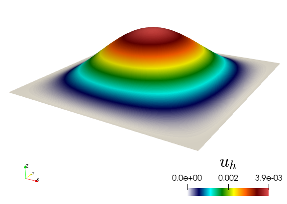
Figure 5.1: Example 1. Approximate solution computed with the C⁰IP on a mesh with $h=0.031$.

Scheme	$\underset{n\in\{{0,1,\cdots,N}\}}{\max}\|e_{h}^{n}\|$	$\underset{n\in\{{0,1,\cdots,N}\}}{\max}\|e_{h}^{n}\|_{h}$	Penalty parameters
Morley	$\underset{n\in\{{0,1,\cdots,N}\}}{\max}\lVert u(t_{n})-U^{n}\rVert$	$\underset{n\in\{{0,1,\cdots,N}\}}{\max}|\!|\!|u(t_{n})-U^{n}|\!|\!|_{\text{\rm pw}}$	No parameter
$\int^{X}_{X}$ dG	$\underset{n\in\{{0,1,\cdots,N}\}}{\max}\lVert u(t_{n})-U^{n}\rVert$	$\underset{n\in\{{0,1,\cdots,N}\}}{\max}\|u(t_{n})-U^{n}\|_{\rm{dG}}$	$\sigma_{\rm dG}^{1}=10,\;\sigma_{\rm dG}^{2}=15$
$\int^{X}_{X}$ $C^{0}$IP	$\underset{n\in\{{0,1,\cdots,N}\}}{\max}\lVert u(t_{n})-U^{n}\rVert$	$\underset{n\in\{{0,1,\cdots,N}\}}{\max}\|u(t_{n})-U^{n}\|_{\rm{IP}}$	$\sigma_{\rm IP}=10$

Table 5.1: Example 1. Error norms and penalty parameter values for different types of spatial discretizations.

	$h$	$L^{2}-$norm	Rate	Energy norm	Rate
Morley	0.250	3.01e-03	–	8.75e-02	–
	0.125	7.95e-04	1.912	4.86e-02	0.793
	0.062	2.12e-04	1.954	2.22e-02	0.898
	0.031	5.33e-05	1.903	1.23e-02	0.931
	0.016	1.41e-05	1.943	6.10e-03	0.965
dG	0.250	2.90e-03	–	1.45e-01	–
	0.125	5.36e-04	1.907	6.96e-02	0.782
	0.062	1.38e-04	1.958	4.36e-02	0.676
	0.031	3.26e-05	2.081	2.06e-02	1.080
	0.016	7.82e-06	2.059	8.51e-03	1.277
$C^{0}$IP	0.250	1.30e-03	–	6.64e-02	–
	0.125	5.12e-04	1.348	3.21e-02	1.051
	0.062	1.52e-04	1.749	1.50e-02	1.096
	0.031	4.04e-05	1.917	7.16e-03	1.066
	0.016	1.03e-05	1.974	3.49e-03	1.038

Table 5.2: Example 1. Error history (errors in the $L^{2}$ and energy norms and estimated convergence rates) associated with the explicit version of the scheme for different discretizations in space.

	$h$	$L^{2}-$norm	Rate	Energy norm	Rate
Morley	0.250	1.48e-03	–	4.51e-02	–
	0.125	6.02e-04	1.301	3.76e-02	0.260
	0.062	2.00e-04	1.586	2.35e-02	0.677
	0.031	5.22e-05	1.942	1.30e-02	0.857
	0.016	1.32e-05	1.978	6.70e-03	0.956
	0.008	3.31e-06	1.997	3.40e-03	0.975
dG	0.250	8.39e-04	–	8.99e-02	–
	0.125	4.22e-04	0.992	6.91e-02	0.378
	0.062	1.32e-04	1.673	4.49e-02	0.625
	0.031	3.19e-05	2.050	2.20e-02	1.031
	0.016	7.79e-06	2.035	9.49e-03	1.211
	0.008	1.94e-06	2.006	4.27e-03	1.153
$C^{0}$IP	0.250	7.11e-04	–	5.15e-02	–
	0.125	4.20e-04	0.759	2.61e-02	0.979
	0.062	1.43e-04	1.557	1.39e-02	0.908
	0.031	3.94e-05	1.859	6.84e-03	1.025
	0.016	1.01e-05	1.967	3.40e-03	1.006
	0.008	2.58e-06	1.968	1.70e-03	1.003

Table 5.3: Example 1. Error history (errors in the $L^{2}$ and energy norms and experimental convergence rates) associated with the implicit version of the scheme for different discretizations in space.

5.2 Example 2: vibration in heterogeneous media

The aim of this section is to illustrate that lowest-order nonstandard methods can effectively address a slightly more complex problem. For this we follow a similar approach as in [3] and consider the following modified PDE

$$u_{tt}(x,t)+\Delta(c(x)\Delta u(x,t))=f(x,t),\quad(x,t)\in\Omega\times\left(0,T\right],$$

with initial and clamped boundary conditions

$$u(x,0)=u^{0}(x),\quad u_{t}(x,0)=v^{0}(x)\text{ in }\Omega;\quad u=\frac{\partial u}{\partial n}=0\text{ on }\partial\Omega\times\left(0,T\right],$$

where the positive coefficient $c$ characterizes the rigidity of the material being considered. The setting adopted for the experiment is

$$\Omega=(-1,1)^{2},\qquad T=\frac{3}{100},\qquad c(x)=\begin{cases}1,&\text{if }x_{2}<0.2,\\ 9,&\text{if }x_{2}\geq 0.2,\end{cases}\qquad f=0,$$

with the initial values

$$u^{0}=\frac{1}{5}\exp(-|10x|^{2})[(1-x_{1}^{2})^{2}(1-x_{2}^{2})^{2}],\qquad v^{0}=0.$$

Figure 5.2: Example 2. Piecewise constant function $c(x_{1},x_{2})$ in the domain $\Omega=(-1,1)^{2}$.

The initial value is a regularized Dirac impulse and stimulates the system’s dynamics. As in the aforementioned reference, we define the control region $\Omega_{c}=(0.75-l_{c},0.75+l_{c})\times(-l_{c},l_{c})$ with $l_{c}=1/32$ (see the small green shaded region in Figure 5.2) that simulates a sensor and evaluate the expression

$$u_{c}(t)=\int_{\Omega_{c}}u_{h}(x,t)\,\mathrm{d}x.$$

Our focus is to examine and compare the signal arrival at the sensor position for different grid and time step sizes for all the three lowest-order schemes discussed in Section 5.1. The calculations were performed on a fixed $50\times 50$ and $100\times 100$. The time steps we chosen as $k=T/N$, where $N$ denotes the number time subintervals. The numerically computed control quantity is presented in Fig. 5.3 (for Morley), Fig. 5.4 (for dG) and Fig. 5.5 (for C⁰IP). Similar graphs can be seen for different time step sizes for corresponding lowest-order schemes which shows the accuracy of schemes. For reference we also plot a warp of the domain by the scalar solution in Fig. 5.6.

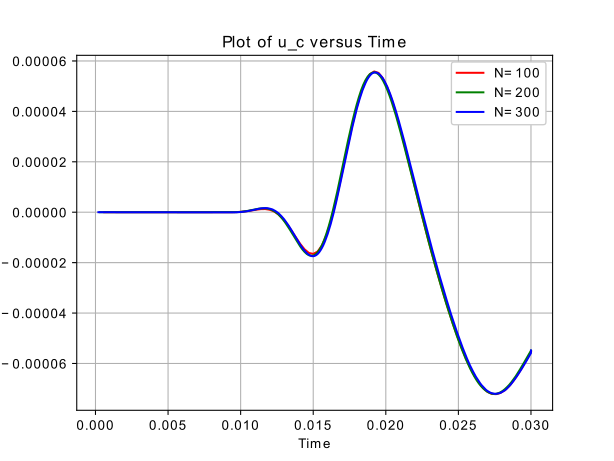
(a)

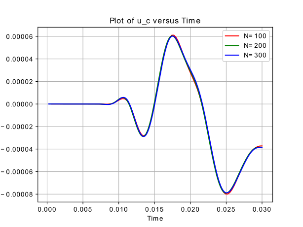
(b)

Figure 5.3: Example 2. Output quantity $u_{c}(t)$ on a $50\times 50$ (left) and $100\times 100$ (right) grid, computed with the Morley scheme.

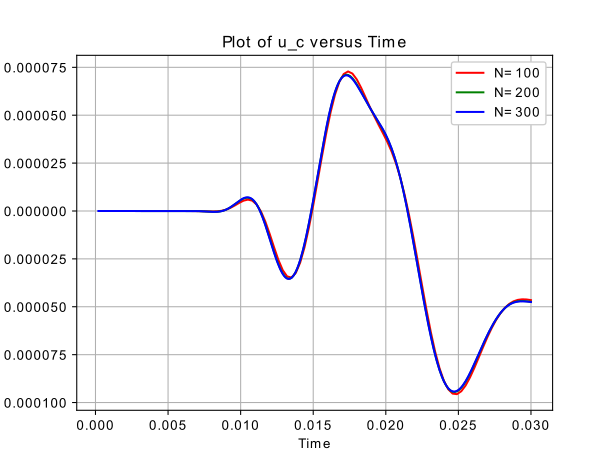
(a)

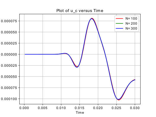
(b)

Figure 5.4: Example 2. Output quantity $u_{c}(t)$ on a $50\times 50$ (left) and $100\times 100$ (right) grid, computed with the dG scheme with $\sigma^{1}_{\text{dG}}=\sigma^{2}_{\text{dG}}=20$.

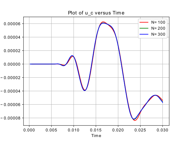
(a)

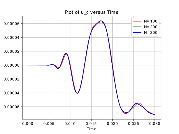
(b)

Figure 5.5: Example 2. Output quantity $u_{c}(t)$ on a $50\times 50$ (left) and $100\times 100$ (right) grid, computed with the C⁰IP scheme with $\sigma_{\text{IP}}=10$.

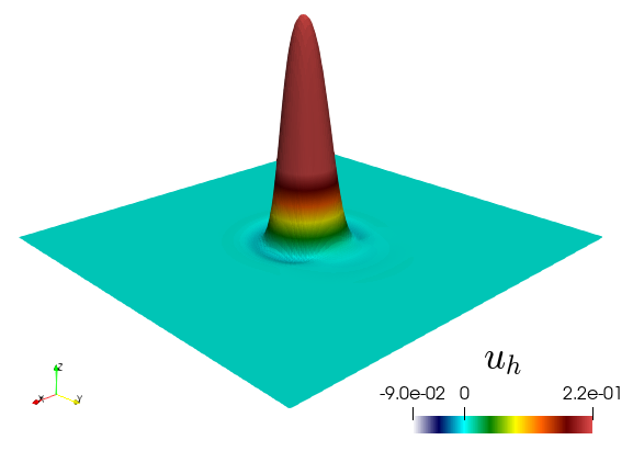
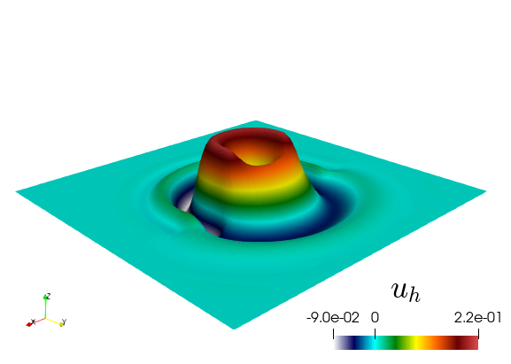
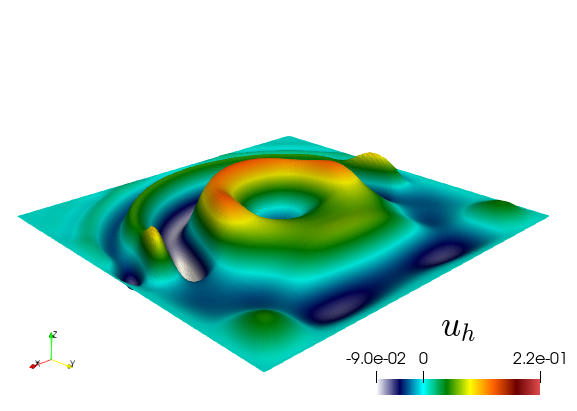
Figure 5.6: Example 2. Snapshots of the approximate solution computed with the dG scheme, and shown at three different time steps.

Appendix A Appendix

A.1 Error analysis of explicit scheme using semidiscrete error bounds

In this section error estimates for the explicit scheme are obtained by using semidiscrete estimates rather than a direct approach used in Section 3.2. We split the error as

$$u(t_{n})-U^{n}=(u(t_{n})-{\cal R}_{h}u(t_{n}))+({\cal R}_{h}u(t_{n})-u_{h}(t_{n}))+(u_{h}(t_{n})-U^{n}):=\rho^{n}+\theta^{n}+\chi^{n}.$$

Recall ${\widetilde{\tau}}^{n}$ is defined in Lemma 3.2. A combination of (2.3) and (3.4) yields the error equation in $\chi^{n}$ as

$$(\partial^{2}_{t}\chi^{n},v_{h})+a_{h}(\chi^{n},v_{h})=({\widetilde{\tau}}^{n},v_{h})\text{ for all }v_{h}\in V_{h}.$$ (A.1)

Recall that $\phi^{1/2}=(\phi^{0}+\phi^{1})/2$. The next lemma establishes the bounds on initial error $\chi^{1/2}:=u_{h}^{1/2}-U^{1/2}$.

Lemma A.1 (Initial error bounds).

For $\gamma_{0}\in(1/2,1]$, the initial error $\chi^{1/2}:=u_{h}^{1/2}-U^{1/2}$ satisfies

$$\lVert\bar{\partial}_{t}\chi^{1/2}\rVert^{2}+\lVert\chi^{1/2}\rVert_{h}^{2}\lesssim{k^{4}}\lVert u_{httt}\rVert^{2}_{L^{\infty}(L^{2}(\Omega))}+h^{4\gamma_{0}}\lVert v^{0}\rVert^{2}_{{H^{2+\gamma_{0}}(\Omega)}},$$

where the constant in “$\lesssim$” depends on $\alpha$ from (2.2) and $C_{2}$ from (2.4).

Proof.

For any $v_{h}\in V_{h}$, the formulations (2.3) and (3.3) show

$$2k^{-1}(\bar{\partial}_{t}\chi^{1/2},v_{h})+a_{h}(\chi^{1/2},v_{h}) =2k^{-1}(\bar{\partial}_{t}u_{h}^{1/2},v_{h})+a_{h}(u_{h}^{1/2},v_{h})-2k^{-1}(\bar{\partial}_{t}U^{1/2},v_{h})-a_{h}(U^{1/2},v_{h})$$

$$=2k^{-1}(\bar{\partial}_{t}u_{h}^{1/2},v_{h})+a_{h}(u_{h}^{1/2},v_{h})-(f^{1/2}+2k^{-1}v^{0},v_{h})$$

$$=({\widetilde{R}}^{0},v_{h})+2k^{-1}(\rho_{t}^{0},v_{h})$$ (A.2)

with ${\widetilde{R}}^{0}:=2k^{-1}(\bar{\partial}^{2}_{t}u_{h}^{1/2}-u_{ht}^{0})-u_{htt}^{1/2}$ from Lemma 3.1 and $\rho_{t}^{0}=u_{ht}^{0}-v^{0}={\cal R}_{h}v^{0}-v^{0}$.
Choose $v_{h}=\chi^{1/2}$ in (A.2) and utilize $2k^{-1}\chi^{1/2}=\bar{\partial}_{t}\chi^{1/2}$ (since $\chi^{0}={\cal{R}}_{h}u^{0}-U^{0}=0$) to obtain

$$(\bar{\partial}_{t}\chi^{1/2},\bar{\partial}_{t}\chi^{1/2})+a_{h}(\chi^{1/2},\chi^{1/2})=\frac{1}{2}k({\widetilde{R}}^{0},\bar{\partial}_{t}\chi^{1/2})+(\rho_{t}^{0},\bar{\partial}_{t}\chi^{1/2}).$$

The ellipticity of $a_{h}(\cdot,\cdot)$ from (2.2) and Cauchy–Schwarz inequality reveal

$$\lVert\bar{\partial}_{t}\chi^{1/2}\rVert^{2}+\alpha\lVert\chi^{1/2}\rVert_{h}^{2} \leq\frac{1}{2}k\lVert{\widetilde{R}}^{0}\rVert\lVert\bar{\partial}_{t}\chi^{1/2}\rVert+\lVert\rho_{t}^{0}\rVert\lVert\bar{\partial}_{t}\chi^{1/2}\rVert.$$ (A.3)

The Young’s inequality (applied twice) with $a=k\lVert{\widetilde{R}}^{0}\rVert$ (resp. $a=\lVert\rho_{t}^{0}\rVert$), $b=\lVert\bar{\partial}_{t}\chi^{1/2}\rVert$ (resp. $b=\lVert\bar{\partial}_{t}\chi^{1/2}\rVert$), $\epsilon=1$ (resp. $\epsilon=2$) for first (resp. second) term on the right-hand side of (A.3) show

$$\frac{1}{2}k\lVert{\widetilde{R}}^{0}\rVert\lVert\bar{\partial}_{t}\chi^{1/2}\rVert+\lVert\rho_{t}^{0}\rVert\lVert\bar{\partial}_{t}\chi^{1/2}\rVert\leq\frac{1}{4}k^{2}\lVert{\widetilde{R}}^{0}\rVert^{2}+\lVert\rho_{t}^{0}\rVert^{2}+\frac{1}{2}\lVert\bar{\partial}_{t}\chi^{1/2}\rVert^{2}.$$ (A.4)

A combination of (A.3) and (A.4) with bounds for ${\widetilde{R}}^{0}$ from Lemma 3.1 and $\rho_{t}^{0}$ from Lemma 2.4 conclude the proof. ∎

The next theorem gives the error bounds under the CFL condition on mesh ratio discussed in Theorem 3.5.

Theorem A.2 (Error estimates).

Consider a quasi-uniform triangulation ${\mathcal{T}_{h}}$ of $\bar{\Omega}$ and assume that the regularity results in Lemma 1.1 and CFL condition $k\leq{\beta^{-1/2}C^{-1}_{\text{\rm inv}}}h^{2}$, hold. Then for $1\leq m\leq N-1$ and $\gamma_{0}\in(1/2,1]$,

$$\lVert\bar{\partial}_{t}u^{m+1/2}-\bar{\partial}_{t}U^{m+1/2}\rVert+\lVert u^{m+1/2}-U^{m+1/2}\rVert_{h}\lesssim h^{\gamma_{0}}L_{(f,u)}+k^{2}M_{(u_{h})},$$

where $L_{(f,u)}$ is given in (2.13), $M_{(u)}:=\lVert u_{ttt}\rVert_{L^{\infty}{(L^{2}(\Omega))}}+\lVert u_{tttt}\rVert_{L^{2}{(L^{2}(\Omega))}},$ and the constant absorbed in ”$\lesssim$” depends on $\alpha$, $\beta$ from (2.2), $T$, and $C_{1}$, $C_{2}$ from Lemmas 2.3-2.4.

Proof.

Choose $v_{h}=2k\delta_{t}\chi^{n}=2(\chi^{n+1/2}-\chi^{n-1/2})=k(\bar{\partial}_{t}\chi^{n+1/2}+\bar{\partial}_{t}\chi^{n-1/2})$ in (A.1) and repeat the arguments in Theorem 3.5 with $U^{n}$ replaced by $\chi^{n}$ and $f^{n}$ by ${\widetilde{\tau}}^{n}$ to arrive at

$$\lVert\bar{\partial}_{t}\chi^{m+1/2}\rVert^{2}+\lVert\chi^{m+1/2}\rVert_{h}^{2}\lesssim\lVert\bar{\partial}_{t}\chi^{1/2}\rVert^{2}+\lVert\chi^{1/2}\rVert_{h}^{2}+Tk\sum_{n=1}^{m}\lVert{\widetilde{\tau}}^{n}\rVert^{2}+k/T\sum_{n=0}^{m-1}\lVert\bar{\partial}_{t}\chi^{n+1/2}\rVert^{2}.$$

The first two terms on the right-hand side of the above expression are bounded using Lemma A.1 and the truncation error $\widetilde{\tau}^{n}$ is bounded using Lemma 3.2. Then we apply the discrete Grönwall Lemma 3.4 to deduce

$$\lVert\bar{\partial}_{t}\chi^{m+1/2}\rVert^{2}+\lVert\chi^{m+1/2}\rVert_{h}^{2}\lesssim k^{4}\lVert u_{httt}\rVert^{2}_{L^{\infty}(L^{2}(\Omega))}+k^{4}\lVert u_{htttt}\rVert^{2}_{L^{2}(L^{2}(\Omega))}+h^{4\gamma_{0}}\lVert v^{0}\rVert^{2}_{H^{2+\gamma_{0}}(\Omega)}.$$

A triangle inequality then shows that $\lVert\bar{\partial}_{t}u^{m+1/2}-\bar{\partial}_{t}U^{m+1/2}\rVert+\lVert u^{m+1/2}-U^{m+1/2}\rVert_{h}\leq\|\rho^{m+1/2}\|+\|\theta^{m+1/2}\|+\|\chi^{m+1/2}\|+\|\bar{\partial}_{t}\rho^{m+1/2}\|+\|\bar{\partial}_{t}\theta^{m+1/2}\|+\|\bar{\partial}_{t}\chi^{m+1/2}\|$. Therefore the proof is completed after using the last displayed estimate, Theorem 2.7, and Lemma 2.4. ∎

A.2 Regularity

This section is devoted to the proof of Lemma 1.1 following the approach from [14, Theorem 12.3]. First, we recall that $\left\{\psi_{n}\right\}_{n=1}^{\infty}$ is an orthonormal basis of $L^{2}(\Omega)$, and hence (cf. [17, Chapter 1, Theorem 4.13])

$$u(x,t)=\sum_{n=1}^{\infty}d_{n}(t)\psi_{n}\text{ and }u_{tt}(x,t)=\sum_{n=1}^{\infty}d^{\prime\prime}_{n}(t)\psi_{n},$$ (A.5)

where $d_{n}(t):=(u,\psi_{n})$ and $d_{n}^{\prime\prime}(t)=(u_{tt},\psi_{n})$. A combination of (1.1) and (A.5) and the fact that $\psi_{n}$’s are smooth functions satisfying (1.4) reveal that for every $j\geq 1$,

$$(f,\psi_{j})=\sum_{n=1}^{\infty}\left(d^{\prime\prime}_{n}(t)\psi_{n},\psi_{j}\right)+\sum_{n=1}^{\infty}\left(\Delta^{2}d_{n}(t)\psi_{n},\psi_{j}\right)=\sum_{n=1}^{\infty}d^{\prime\prime}_{n}(t)\left(\psi_{n},\psi_{j}\right)+\sum_{n=1}^{\infty}d_{n}(t)\left(\lambda_{n}\psi_{n},\psi_{j}\right).$$

The orthonormality of the $\psi_{n}$’s simplifies the above equation to a second-order linear ODE as

$$d_{j}^{\prime\prime}+\lambda_{j}d_{j}=f_{j}\text{ with }d_{j}(0)=(u(0),\psi_{j})=(u^{0},\psi_{j}),\;d_{j}^{\prime}(0)=(u_{t}(0),\psi_{j})=(v^{0},\psi_{j}),\;\text{and }f_{j}(t)=(f(t),\psi_{j}),$$

for all $t\in[0,T]$. For $n\geq 1$, the solution of this ODE is

$$d_{n}(t)=(u^{0},\psi_{n})\cos\sqrt{\lambda_{n}}t+\lambda_{n}^{-1/2}{(v^{0},\psi_{n})}\sin\sqrt{\lambda_{n}}t+\lambda_{n}^{-1/2}I(t),$$ (A.6)

where $\displaystyle I(t):=\int_{0}^{t}\sin\sqrt{\lambda_{n}}(t-s)f_{n}(s)\,\mathrm{d}s.$ A successive differentiation with respect to $t$ shows that

$$I^{\prime}(t) =\sqrt{\lambda_{n}}\int_{0}^{t}\cos\sqrt{\lambda_{n}}(t-s)f_{n}(s)\,\mathrm{d}s\text{ and }I^{\prime\prime}(t)=\sqrt{\lambda}_{n}f_{n}(t)-{\lambda_{n}}\int_{0}^{t}\sin\sqrt{\lambda_{n}}(t-s)f_{n}(s)\,\mathrm{d}s.$$

Then we can apply integration by parts thrice to the term $I^{\prime\prime}(t)$ shown above, to observe the following

$$I^{\prime\prime}(t) =\sqrt{\lambda}_{n}f_{n}(0)\cos\sqrt{\lambda}_{n}t+\sqrt{\lambda}_{n}\int_{0}^{t}f^{\prime}_{n}(s)\cos\sqrt{\lambda}_{n}(t-s)\,\mathrm{d}s,$$ (A.7a)

$$I^{\prime\prime}(t) =\sqrt{\lambda_{n}}f_{n}(0)\cos\sqrt{\lambda_{n}}t+{f^{\prime}_{n}(0)}\sin\sqrt{\lambda_{n}}t+\int_{0}^{t}f^{\prime\prime}_{n}(s)\sin\sqrt{\lambda_{n}}(t-s)\,\mathrm{d}s,$$ (A.7b)

$$I^{\prime\prime}(t) =\sqrt{\lambda_{n}}f_{n}(0)\cos\sqrt{\lambda_{n}}t+{f^{\prime}_{n}(0)}\sin\sqrt{\lambda_{n}}t-{\lambda_{n}^{-1/2}}{f^{\prime\prime}_{n}(0)}\cos\sqrt{\lambda_{n}}t$$

$$\qquad+\lambda_{n}^{-1/2}f^{\prime\prime}_{n}(t)-\lambda_{n}^{-1/2}\int_{0}^{t}\cos\sqrt{\lambda_{n}}(t-s)f^{\prime\prime\prime}_{n}(s)\,\mathrm{d}s.$$ (A.7c)

The expressions in (A.7) are utilized appropriately to control $u_{tt}$ in the $L^{2}(\Omega)$ and $H^{2+\gamma_{0}}(\Omega)$ norms. In addition, the integration by parts is aimed at reducing the spatial regularity of $f$ and its time derivatives. Next, we proceed to differentiate (A.6) twice and use (1.5) (with $D(A^{0})=L^{2}(\Omega)$), which leads to

$$\lVert u_{tt}\rVert^{2}=\sum_{n=1}^{\infty}|(u_{tt},\psi_{n})|^{2} =\sum_{n=1}^{\infty}|d^{\prime\prime}_{n}(t)|^{2}$$

$$=\sum_{n=1}^{\infty}|-\lambda_{n}(u^{0},\psi_{n})\cos\sqrt{\lambda_{n}}t-\sqrt{\lambda_{n}}{(v^{0},\psi_{n})}\sin\sqrt{\lambda_{n}}t+{{\lambda_{n}}}^{-1/2}I^{\prime\prime}(t)|^{2}.$$ (A.8)

A combination of this with (A.7a), a use of the definitions of $f_{n},f_{n}^{\prime}$, with elementary manipulations show

$$\lVert u_{tt}\rVert^{2} \lesssim\sum_{n=1}^{\infty}\left(|\lambda_{n}(u^{0},\psi_{n})|^{2}+|\sqrt{\lambda_{n}}(v^{0},\psi_{n})|^{2}+|f_{n}(0)\cos\sqrt{\lambda_{n}}t+\int_{0}^{t}f^{\prime}_{n}(s)\cos\sqrt{\lambda_{n}}(t-s)\,\mathrm{d}s|^{2}\right)$$

$$\lesssim\sum_{n=1}^{\infty}\left(|\lambda_{n}(u^{0},\psi_{n})|^{2}+|\sqrt{\lambda_{n}}(v^{0},\psi_{n})|^{2}+\left|(f(0),\psi_{n})\right|^{2}+\int_{0}^{t}|(f^{\prime}(s),\psi_{n})|^{2}\,\mathrm{d}s\right).$$ (A.9)

Since $f_{t}\in L^{2}(\Omega)$, an application of the monotone convergence theorem and (1.5) shows

$$\lVert u_{tt}\rVert^{2}_{L^{\infty}(L^{2}(\Omega))}\lesssim\left(\lVert u^{0}\rVert^{2}_{D(A)}+\lVert v^{0}\rVert^{2}_{D(A^{1/2})}+\lVert f(0)\rVert^{2}+\lVert f_{t}\rVert^{2}_{L^{2}(L^{2}(\Omega))}\right).$$ (A.10)

Then we differentiate (A.6) thrice (resp. four times) to obtain

$$d^{\prime\prime\prime}_{n}(t) =\lambda_{n}^{3/2}(u^{0},\psi_{n})\sin\sqrt{\lambda_{n}}t-\lambda_{n}(v^{0},\psi_{n})\cos\sqrt{\lambda_{n}}t+{{\lambda_{n}}}^{-1/2}I^{\prime\prime\prime}(t)$$

$$\big{(}\text{resp. }d^{\prime\prime\prime\prime}_{n}(t) =\lambda_{n}^{2}(u^{0},\psi_{n})\cos\sqrt{\lambda_{n}}t+\lambda_{n}^{3/2}(v^{0},\psi_{n})\sin\sqrt{\lambda_{n}}t+{{\lambda_{n}}}^{-1/2}I^{\prime\prime\prime\prime}(t)\big{)}.$$

An integration by parts twice (resp. thrice) to the last term $I^{\prime\prime\prime}(t)$ (resp. $I^{{}^{\prime\prime\prime\prime}}(t)$) leads to

$$d^{\prime\prime\prime}_{n}(t) =\lambda_{n}^{3/2}(u^{0},\psi_{n})\sin\sqrt{\lambda_{n}}t-\lambda_{n}(v^{0},\psi_{n})\cos\sqrt{\lambda_{n}}t-\sqrt{\lambda_{n}}\sin\sqrt{\lambda_{n}}tf_{n}(0)$$

$$\quad+\cos\sqrt{\lambda_{n}}tf^{\prime}_{n}(0)+\int_{0}^{t}\cos\sqrt{\lambda_{n}}(t-s)f^{\prime\prime}_{n}(s)\,\mathrm{d}s.$$

$$\big{(}\text{resp. }d^{\prime\prime\prime\prime}_{n}(t) =\lambda_{n}^{2}(u^{0},\psi_{n})\cos\sqrt{\lambda_{n}}t+\lambda_{n}^{3/2}(v^{0},\psi_{n})\sin\sqrt{\lambda_{n}}t-\lambda_{n}\cos\sqrt{\lambda_{n}}tf_{n}(0)$$

$$\quad-\sqrt{\lambda_{n}}\sin\sqrt{\lambda_{n}}tf^{\prime}_{n}(0)+\cos\sqrt{\lambda_{n}}f^{\prime\prime}_{n}(0)+\int_{0}^{t}\cos\sqrt{\lambda_{n}}(t-s)f^{\prime\prime\prime}_{n}(s)\,\mathrm{d}s\big{)}.$$

The fact that $\lVert u_{ttt}\rVert^{2}=\sum_{n=1}^{\infty}|d^{\prime\prime\prime}_{n}(t)|^{2}$ (resp. $\lVert u_{tttt}\rVert^{2}=\sum_{n=1}^{\infty}|d^{\prime\prime\prime\prime}_{n}(t)|^{2}$) from (1.5) and an approach similar to (A.8)-(A.10) leads to

$$\lVert u_{ttt}\rVert^{2}_{L^{\infty}(L^{2}(\Omega))} \lesssim\lVert u^{0}\rVert^{2}_{D(A^{3/2})}+\lVert v^{0}\rVert^{2}_{D(A)}+\lVert f(0)\rVert^{2}_{D(A^{1/2})}+\lVert f_{t}(0)\rVert^{2}+\lVert f_{tt}\rVert^{2}_{L^{2}(L^{2}(\Omega))},$$

$$\lVert u_{tttt}\rVert^{2}_{L^{\infty}(L^{2}(\Omega))} \lesssim\lVert u^{0}\rVert^{2}_{D(A^{2})}+\lVert v^{0}\rVert^{2}_{D(A^{3/2})}+\lVert f(0)\rVert^{2}_{D(A)}+\lVert f_{t}(0)\rVert_{D(A^{1/2})}^{2}+\lVert f_{tt}(0)\rVert^{2}+\lVert f_{ttt}\rVert^{2}_{L^{2}(L^{2}(\Omega))}.$$

Now we aim to control $\|u_{tt}\|_{D(A)}$. A differentiation of (A.6) twice and substitution of $d^{\prime\prime}_{n}(t)$ in (A.5) shows

$$\lVert u_{tt}\rVert^{2}_{D(A)}=\sum_{n=1}^{\infty}|\lambda_{n}d_{n}^{\prime\prime}(t)|^{2}=\sum_{n=1}^{\infty}\left|-\lambda_{n}^{2}(u^{0},\psi_{n})\cos\sqrt{\lambda_{n}}t-\lambda_{n}^{3/2}{(v^{0},\psi_{n})}\sin\sqrt{\lambda_{n}}t+{\lambda_{n}^{1/2}}I^{\prime\prime}(t)\right|^{2}.$$ (A.11)

We can then argue as before by using (A.7c) to conclude that, for any $t\in[0,T],$

$$\lVert u_{tt}\rVert^{2}_{L^{\infty}({H^{2+\gamma_{0}}(\Omega))}} \lesssim\sum_{n=1}^{\infty}\left(|\lambda_{n}^{2}(u^{0},\psi_{n})|^{2}+\left|\lambda_{n}^{3/2}{(v^{0},\psi_{n})}\right|^{2}+|\lambda_{n}f_{n}(0)|^{2}+|\sqrt{\lambda_{n}}f^{\prime}_{n}(0)|^{2}\right.$$

$$\left.\qquad\qquad+|{f^{\prime\prime}_{n}(0)}|^{2}+|f^{\prime\prime}_{n}(t)|^{2}+\int_{0}^{t}|f^{\prime\prime\prime}_{n}(s)|^{2}\,\mathrm{d}s\right).$$

As $f,\;f_{t},\;f_{tt},\text{ and }f_{ttt}\in L^{2}(L^{2}(\Omega))$, from the Sobolev embedding we can infer that $f,\;f_{t},\text{ and }f_{tt}\in L^{\infty}(L^{2}(\Omega))$. Consequently, (1.5) and the fact that $D(A)\subset H^{2+\gamma_{0}}(\Omega)$ (i.e., $\lVert u_{tt}\rVert^{2}_{H^{2+\gamma_{0}}(\Omega)}\leq\lVert u_{tt}\rVert^{2}_{D(A)})$, show that $\lVert u_{tt}\rVert^{2}_{H^{2+\gamma_{0}}(\Omega)}$ is bounded (up to a multiplicative constant) by

$$\lVert u^{0}\rVert^{2}_{D(A^{2})}+\lVert v^{0}\rVert^{2}_{D(A^{3/2})}+\lVert f(0)\rVert^{2}_{D(A)}+\lVert f_{t}(0)\rVert^{2}_{D(A^{1/2})}+\lVert f_{tt}(0)\rVert^{2}+\lVert f_{tt}\rVert^{2}_{L^{\infty}(L^{2}(\Omega))}+\lVert f_{ttt}\rVert^{2}_{L^{2}(L^{2}(\Omega))}.$$ (A.12)

Finally, (A.6) with integration by parts applied to the last term $I(t)$ once, and a differentiation of (A.6) once followed by integration by parts of the term $I^{\prime}(t)$ appearing in the derivative twice, yields

$$d_{n}(t) =(u^{0},\psi_{n})\cos\sqrt{\lambda_{n}}t+\lambda_{n}^{-1/2}{(v^{0},\psi_{n})}\sin\sqrt{\lambda_{n}}t+\lambda_{n}^{-1}f_{n}(t)$$

$$\quad-\lambda_{n}^{-1}\cos\sqrt{\lambda_{n}}tf_{n}(0)-\lambda_{n}^{-1}\int_{0}^{t}\cos\sqrt{\lambda_{n}}(t-s)f^{\prime}_{n}(s)\,\mathrm{d}s.$$

$$\big{(}\text{resp. }d^{\prime}_{n}(t) =-\sqrt{\lambda_{n}}(u^{0},\psi_{n})\sin\sqrt{\lambda_{n}}t+{(v^{0},\psi_{n})}\cos\sqrt{\lambda_{n}}t+\lambda_{n}^{-1/2}\sin\sqrt{\lambda_{n}}tf_{n}(0)$$

$$\quad+\lambda_{n}^{-1}f^{\prime}_{n}(t)-\lambda_{n}^{-1}\cos\sqrt{\lambda_{n}}tf^{\prime}_{n}(0)-\lambda_{n}^{-1}\int_{0}^{t}\cos\sqrt{\lambda_{n}}(t-s)f^{\prime\prime}_{n}(s)\,\mathrm{d}s\big{)}.$$

An analogous approach to that used to obtain (A.12) from (A.11), readily shows that

$$\lVert u\rVert^{2}_{L^{\infty}({H^{2+\gamma_{0}}(\Omega))}} \lesssim\lVert u^{0}\rVert^{2}_{D(A)}+\lVert v^{0}\rVert^{2}_{D(A^{1/2})}+\lVert f(0)\rVert^{2}+\lVert f\rVert^{2}_{L^{\infty}(L^{2}(\Omega))}+\lVert f_{t}\rVert^{2}_{L^{2}(L^{2}(\Omega))},$$

$$\lVert u_{t}\rVert^{2}_{L^{\infty}({H^{2+\gamma_{0}}(\Omega))}} \lesssim\lVert u^{0}\rVert^{2}_{D(A^{3/2})}+\lVert v^{0}\rVert^{2}_{D(A)}+\lVert f(0)\rVert^{2}_{D(A^{1/2})}+\lVert f_{t}(0)\rVert^{2}+\lVert f_{t}\rVert^{2}_{L^{\infty}(L^{2}(\Omega))}+\lVert f_{tt}\rVert^{2}_{L^{2}(L^{2}(\Omega))},$$

and this concludes the proof. ∎

References

• [1] M. S. Alnæs, J. Blechta, J. Hake, A. Johansson, B. Kehlet, A. Logg, C. Richardson, J. Ring, M. E. Rognes, and G. N. Wells, The FEniCS project version 1.5, Arch. Numer. Softw., 3 (2015).
• [2] I. Babuška and J. Osborn, Eigenvalue problems, in Handbook of numerical analysis, Vol. II, vol. II of Handb. Numer. Anal., North-Holland, Amsterdam, 1991, pp. 641–787.
• [3] M. Bause, M. Lymbery, and K. Osthues, $C^{1}$-conforming variational discretization of the biharmonic wave equation, Comput. Math. Appl., 119 (2022), pp. 208–219.
• [4] E. Bécache, G. Derveaux, and P. Joly, An efficient numerical method for the resolution of the Kirchhoff-Love dynamic plate equation, Numer. Methods Partial Differential Equations, 21 (2005), pp. 323–348.
• [5] H. Blum and R. Rannacher, On the boundary value problem of the biharmonic operator on domains with angular corners, Math. Methods Appl. Sci., 2 (1980), pp. 556–581.
• [6] D. Braess, A. S. Pechstein, and J. Schöberl, An equilibration-based a posteriori error bound for the biharmonic equation and two finite element methods, IMA J. Numer. Anal., 40 (2020), pp. 951–975.
• [7] S. C. Brenner and L. R. Scott, The mathematical theory of finite element methods, vol. 15 of Texts in Applied Mathematics, Springer, New York, third ed., 2008.
• [8] W. Cao, D. Li, and Z. Zhang, Unconditionally optimal convergence of an energy-conserving and linearly implicit scheme for nonlinear wave equations, Sci. China Math., 65 (2022), pp. 1731–1748.
• [9] C. Carstensen, D. Gallistl, and N. Nataraj, Comparison results of nonstandard $P_{2}$ finite element methods for the biharmonic problem, ESAIM Math. Model. Numer. Anal., 49 (2015), pp. 977–990.
• [10] C. Carstensen and N. Nataraj, Adaptive Morley FEM for the von Kármán equations with optimal convergence rates, SIAM J. Numer. Anal., 59 (2021), pp. 696–719.
• [11]  , Lowest-order equivalent nonstandard finite element methods for biharmonic plates, ESAIM Math. Model. Numer. Anal., 56 (2022), pp. 41–78.
• [12] C. Carstensen and S. Puttkammer, How to prove the discrete reliability for nonconforming finite element methods, J. Comput. Math., 38 (2020), pp. 142–175.
• [13] C. Chen and T. Shih, Finite element methods for integrodifferential equations, vol. 9 of Series on Applied Mathematics, World Scientific Publishing Co., Inc., River Edge, NJ, 1998.
• [14]  , Finite element methods for integrodifferential equations, vol. 9 of Series on Applied Mathematics, World Scientific Publishing Co., Inc., River Edge, NJ, 1998.
• [15] C. Chen, X. Zhao, and Y. Zhang, A posteriori error estimate for finite volume element method of the second-order hyperbolic equations, Math. Probl. Eng., (2015), pp. Art. ID 510241, 11.
• [16] P. G. Ciarlet, Mathematical elasticity. Volume II. Theory of plates, vol. 85 of Classics in Applied Mathematics, Society for Industrial and Applied Mathematics (SIAM), Philadelphia, PA, [2022] ©2022. Reprint of the 1997 edition [1477663].
• [17] J. B. Conway, A course in functional analysis, vol. 96 of Graduate Texts in Mathematics, Springer-Verlag, New York, second ed., 1990.
• [18] P. Danumjaya, A. K. Pany, and A. K. Pani, Morley FEM for the fourth-order nonlinear reaction-diffusion problems, Comput. Math. Appl., 99 (2021), pp. 229–245.
• [19] B. Deka and R. K. Sinha, Finite element methods for second order linear hyperbolic interface problems, Appl. Math. Comput., 218 (2012), pp. 10922–10933.
• [20] P. Destuynder and M. Salaun, Mathematical analysis of thin plate models, vol. 24 of Mathématiques & Applications (Berlin) [Mathematics & Applications], Springer-Verlag, Berlin, 1996.
• [21] Z. Dong and A. Ern, Hybrid high-order and weak Galerkin methods for the biharmonic problem, SIAM J. Numer. Anal., 60 (2022), pp. 2626–2656.
• [22] T. Dupont, $L^{2}$-estimates for Galerkin methods for second order hyperbolic equations, SIAM J. Numer. Anal., 10 (1973), pp. 880–889.
• [23] G. Fairweather, Galerkin methods for vibration problems in two space variables, SIAM J. Numer. Anal., 9 (1972), pp. 702–714.
• [24] E. H. Georgoulis and P. Houston, Discontinuous Galerkin methods for the biharmonic problem, IMA J. Numer. Anal., 29 (2009), pp. 573–594.
• [25] E. H. Georgoulis, P. Houston, and J. Virtanen, An a posteriori error indicator for discontinuous Galerkin approximations of fourth-order elliptic problems, IMA J. Numer. Anal., 31 (2011), pp. 281–298.
• [26] E. H. Georgoulis and J. M. Virtanen, Adaptive discontinuous Galerkin approximations to fourth order parabolic problems, Math. Comp., 84 (2015), pp. 2163–2190.
• [27] T. Geveci, On the application of mixed finite element methods to the wave equations, RAIRO Modél. Math. Anal. Numér., 22 (1988), pp. 243–250.
• [28] M. J. Grote, A. Schneebeli, and D. Schötzau, Discontinuous Galerkin finite element method for the wave equation, SIAM J. Numer. Anal., 44 (2006), pp. 2408–2431.
• [29] M. J. Grote and D. Schötzau, Optimal error estimates for the fully discrete interior penalty DG method for the wave equation, J. Sci. Comput., 40 (2009), pp. 257–272.
• [30] T. Gudi and H. S. Gupta, A fully discrete $C^{0}$ interior penalty Galerkin approximation of the extended Fisher-Kolmogorov equation, J. Comput. Appl. Math., 247 (2013), pp. 1–16.
• [31] H. Guo, Z. Zhang, and Q. Zou, A $C^{0}$ linear finite element method for biharmonic problems, J. Sci. Comput., 74 (2018), pp. 1397–1422.
• [32] M. He, J. Tian, P. Sun, and Z. Zhang, An energy-conserving finite element method for nonlinear fourth-order wave equations, Appl. Numer. Math., 183 (2023), pp. 333–354.
• [33] S. He, H. Li, and Y. Liu, Analysis of mixed finite element methods for fourth-order wave equations, Comput. Math. Appl., 65 (2013), pp. 1–16.
• [34] F. Hecht, New development in FreeFem++, J. Numer. Math., 20 (2012), pp. 251–265.
• [35] R. H. W. Hoppe, A $\rm C^{0}$ interior penalty discontinuous Galerkin method and an equilibrated a posteriori error estimator for a nonlinear fourth order elliptic boundary value problem of $p$-biharmonic type, ESAIM Math. Model. Numer. Anal., 56 (2022), pp. 2051–2079.
• [36] C. Johnson, Discontinuous Galerkin finite element methods for second order hyperbolic problems, Comput. Methods Appl. Mech. Engrg., 107 (1993), pp. 117–129.
• [37] J. Lagnese and J.-L. Lions, Modelling analysis and control of thin plates, vol. 6 of Recherches en Mathématiques Appliquées [Research in Applied Mathematics], Masson, Paris, 1988.
• [38] S. Larsson and V. Thomée, Partial differential equations with numerical methods, vol. 45 of Texts in Applied Mathematics, Springer-Verlag, Berlin, 2009. Paperback reprint of the 2003 edition.
• [39] D. Li, C. Wang, and J. Wang, Generalized weak Galerkin finite element methods for biharmonic equations, J. Comput. Appl. Math., 434 (2023), pp. Paper No. 115353, 21.
• [40] Y. Li, Error analysis of a fully discrete Morley finite element approximation for the Cahn-Hilliard equation, J. Sci. Comput., 78 (2019), pp. 1862–1892.
• [41] J.-L. Lions and E. Magenes, Non-homogeneous boundary value problems and applications. Vol. II, vol. Band 182 of Die Grundlehren der mathematischen Wissenschaften, Springer-Verlag, New York-Heidelberg, 1972. Translated from the French by P. Kenneth.
• [42] A. K. Pani, R. K. Sinha, and A. K. Otta, An $H^{1}$-Galerkin mixed method for second order hyperbolic equations, Int. J. Numer. Anal. Model., 1 (2004), pp. 111–130.
• [43] E. Süli and I. Mozolevski, $hp$-version interior penalty DGFEMs for the biharmonic equation, Comput. Methods Appl. Mech. Engrg., 196 (2007), pp. 1851–1863.
• [44] M. Wang and J. Xu, The Morley element for fourth order elliptic equations in any dimensions, Numer. Math., 103 (2006), pp. 155–169.
• [45] X. Ye and S. Zhang, A $C^{0}$-conforming DG finite element method for biharmonic equations on triangle/tetrahedron, J. Numer. Math., 30 (2022), pp. 163–172.