Mixture Modeling for Temporal Point Processes with Memory

Abstract

We propose a constructive approach to building temporal point processes that incorporate dependence on their history. The dependence is modeled through the conditional density of the duration, i.e., the interval between successive event times, using a mixture of first-order conditional densities for each one of a specific number of lagged durations. Such a formulation for the conditional duration density accommodates high-order dynamics, and it thus enables flexible modeling for point processes with memory. The implied conditional intensity function admits a representation as a local mixture of first-order hazard functions. By specifying appropriate families of distributions for the first-order conditional densities, with different shapes for the associated hazard functions, we can obtain either self-exciting or self-regulating point processes. From the perspective of duration processes, we develop a method to specify a stationary marginal density. The resulting model, interpreted as a dependent renewal process, introduces high-order Markov dependence among identically distributed durations. Furthermore, we provide extensions to cluster point processes. These can describe duration clustering behaviors attributed to different factors, thus expanding the scope of the modeling framework to a wider range of applications. Regarding implementation, we develop a Bayesian approach to inference, model checking, and prediction. We investigate point process model properties analytically, and illustrate the methodology with both synthetic and real data examples.

Keywords: Bayesian hierarchical models; Cluster point processes; Copulas; Dependent point processes; Mixture transition distribution models; Self-exciting processes.

1 Introduction

Temporal point processes are stochastic models for sequences of random events that occur in continuous time, with irregular durations, i.e., intervals between successive arrival times. Throughout this article, event time and arrival time will be used interchangeably for the occurrence time of an event. Data corresponding to point patterns are common in a wide range of applications, such as earthquake occurrences (Ogata, 1988), recurrent events (Cook et al., 2007), financial high frequency trading and orders (Hautsch, 2011), and neural spike trains (Tang and Li, 2021), to name a few. For many point patterns, it is believed that occurrence of a future event depends on the past. This motivates the use of point processes with memory, for example, the Hawkes process (Hawkes, 1971) with full memory, or renewal processes with lagged dependence. The goal of this article is to propose a modeling framework for point processes with high-order memory, relaxing the assumption of independent durations in the traditional renewal process, and including the ability to model duration-clustering behaviors present in applications such as health care (Yang et al., 2018), climatology (Cowpertwait, 2001), and finance (O’Hara, 1995).

As such, this article explores construction of point processes based on models for the durations. For point processes with memory, the collection of dependent durations form a discrete-time stochastic process, and thus a time series model for durations induces conditional densities on the arrival times. Hereafter, we refer to these conditional densities as conditional arrival densities, and notice that they uniquely determine the distribution of the resulting point process (Daley and Vere-Jones, 2003). A common approach to model point process dependence is to specify the conditional intensity of the process, namely, the instantaneous event rate conditional on the process history (e.g., the Hawkes process). In fact, a point process can be equivalently characterized by its conditional intensity or the conditional arrival densities. The latter approach benefits from the vast literature on conditional density modeling. Density-based modeling naturally leads to a well-defined point process, with its conditional intensity derived through a normalization of the conditional arrival densities against the associated survival functions (Daley and Vere-Jones, 2003). Constructing point processes using duration models, usually coupled with a limited memory assumption, can be computationally attractive for inference, as this approach facilitates evaluation of the resulting likelihood. In Section 2, we provide further discussion of the duration-based approach that induces conditional arrival densities, as well as its connection to and difference from the conditional intensity approach.

Statistical models for durations date back at least to Wold (1948) who proposed a first-order Markov chain with an additive model representation. Subsequent developments (Jacobs and Lewis, 1977; Gaver and Lewis, 1980) investigate specific families for the duration process stationary marginal distribution. Since durations are positive-valued, a structure with an additive error process is in general restrictive. A popular class of models in finance is built from the autoregressive conditional duration (ACD) structure (Engle and Russell, 1998). The ACD model assumes independent and identically distributed (i.i.d.) multiplicative errors for the durations, with each multiplicative factor modeled as a linear function of the past factors and durations. Extensions of this class of models provide additional flexibility through the multiplicative factor specification or the error distribution choice. We refer to Pacurar (2008) and Bhogal and Thekke Variyam (2019) for comprehensive reviews. For these models, the conditional intensity function is obtained by scaling the baseline hazard function with multiplicative factors. The baseline hazard corresponds to the error distribution, typically chosen within a parametric family. A restriction of ACD models is their limited capacity to handle non-linear dynamics. Moreover, treating point process realizations as time series affects the distributional properties of likelihood-based estimators (Cavaliere et al., 2024). Regarding computation, the ACD model structure complicates inference when the assumption of high-order memory is necessary, e.g., estimating the correlated multiplicative factors may require approximations (Strickland et al., 2006).

A different approach to modeling duration dependence involves mixture transition distribution (MTD) models (Le et al., 1996), which describe the transition density of a time series as a weighted combination of first-order conditional densities for each one of a specified number of lags. Hassan and Lii (2006) propose a bivariate MTD model for the joint conditional distribution of the duration and a continuous mark, i.e., a random variable associated with the point events. Hassan and El-Bassiouni (2013) extend the model to include a discrete mark. However, these approaches do not investigate point process properties, such as stationarity, and require certain families of distributions for the duration and mark, which can be practically restrictive. Hassan and Lii (2006) point out the difficulties of finding suitable parameterizations to ensure model stability and prediction capability.

In this article, we introduce a class of temporal point processes that builds on the idea of describing duration process dynamics with MTD models. To use traditional high-order autoregressive models, a transformation of the durations or their conditional means is typically needed to handle the dependent, positive-valued durations. This introduces the challenge of inference under a constrained, possibly high-dimensional parameter space. For example, coefficients may need to be restricted to avoid negative-valued durations, and implementing stationarity conditions in practice can be difficult, especially under the assumption of high-order dependence. The aforementioned work that uses MTD models attempts to handle the former issue, albeit under restrictive structures. A key contribution of the present article is the development of an MTD point process (MTDPP) constructive framework that provides flexible modeling of high-order dynamics for the duration process, without parameter constraints. The framework allows for various types of practically relevant point patterns, such as those with self-excitation or self-regulation effects. In addition, it provides an efficient inferential approach, as the MTDPP likelihood evaluation grows linearly with the number of events. Thus, our proposed method is computationally scalable, especially for large point patterns with high-order memory.

Within the MTDPP framework, we provide easily-implemented conditions to construct point processes that correspond to pre-specified families of marginal distributions for the durations. In addition, we obtain a limit result for the mean value function, analogous to that for renewal processes. The resulting class of models has identically distributed, high-order dependent durations, and can be interpreted as a class of dependent renewal processes. This relaxes the assumption of independent durations that may be restrictive in practice. To the best of our knowledge, the proposed model is the first to enable simultaneous modeling of high-order dependence and stationary durations, with computationally efficient inference.

Moreover, we develop an extension to handle duration clustering, based on a two-component mixture for the conditional duration density. In this setting, one component of the mixture corresponds to an independent duration model that accounts for external factors. The other component is an MTDPP that models self-excitation. Point patterns of this type can be found, for instance, in hospital emergency department visits of patients, where long durations may be observed between clusters of multiple visits in short bursts (Yang et al., 2018), and in financial markets where fluctuation can be caused by either external or internal processes (Filimonov and Sornette, 2012). The model extension accounts for the possibility of two different factors that may drive the point process dynamics.

The rest of the article is organized as follows. Section 2 introduces the MTDPP framework, including study of model properties, approaches to constructing various types of MTDPP models, and the extension to cluster point processes. (Technical details and proofs of the theoretical results can be found in the Supplementary Material.) Section 3 develops the Bayesian model formulation, Markov chain Monte Carlo (MCMC) inference, an approach for predicting future events, and a model validation method. In Section 4, we illustrate the proposed methodology with synthetic and real data examples. Finally, Section 5 concludes with a summary and discussion.

2 Temporal MTD point processes

We consider a temporal point process $N(t)$ defined on the positive half-line $\mathbb{R}^{+}$, where $N(t)=\sum_{i\geq 1}\mathbbm{1}(\{t_{i}\leq t\})$ is a right-continuous, integer-valued function, $t_{1},t_{2},\ldots\in\mathbb{R}^{+}$ denote the event times, and $\mathbbm{1}(A)$ is the indicator function for set $A$. A temporal point process is usually modeled by its conditional intensity, $\lambda^{*}(t)\equiv\lambda(t\,|\,\mathcal{H}_{t})=\lim_{dt\rightarrow 0}E[dN(t)\,|\,\mathcal{H}_{t}]/dt$, where $dN(t)=N(t+dt)-N(t)$, and $\mathcal{H}_{t}$ is the process history up to but not including $t$. The point process has memory if $\lambda^{*}(t)$ depends on the process history. A Poisson process is an example of a memoryless process. A renewal process has limited memory, in particular, $\mathcal{H}_{t}=t_{N(t^{-})}$, where $t_{N(t^{-})}$ is the most recent arrival time before $t$. In contrast, the evolution of a Hawkes process depends on the entire past. Given an observed sequence of arrival times, $0<t_{1}<\ldots<t_{n}<T$, the likelihood is

$$p(t_{1},\dots,t_{n})=\left(\prod_{i=1}^{n}\lambda^{*}(t_{i})\right)\exp\left(-\int_{0}^{T}\lambda^{*}(t)\,dt\right),$$ (1)

where the last component of (1) corresponds to the point process likelihood’s normalizing term, which is typically analytically intractable, especially when $\lambda^{*}(t)$ has a complicated form. The normalizing term also implies that building point process models through conditional intensities requires mathematical validation of the proposed intensity function.

An alternative way to characterize the point process probability structure is to use the collection of conditional arrival densities, denoted as $p^{*}_{i}(t)\equiv p_{i}(t\,|\,\mathcal{H}_{t})$, supported on $(t_{i-1},\infty)$, with associated conditional survival functions $S^{*}_{i}(t)=$ $1-\int_{t_{i-1}}^{t}p^{*}_{i}(u)du$. When $i=1$, $p_{1}^{*}(t)\equiv p_{1}(t)$ and $S_{1}^{*}(t)=1-\int_{0}^{t}p^{*}_{1}(u)du$, where $p_{1}$ is the marginal density of the first event time. Now, the likelihood for point pattern $0<t_{1}<\ldots<t_{n}<T$ is given by

$$p(t_{1},\dots,t_{n})=\left(\prod_{i=1}^{n}p^{*}_{i}(t_{i})\right)\left(1-\int_{t_{n}}^{T}p^{*}_{n+1}(u)\,du\right).$$ (2)

Similar to (1), the last component of (2) defines the likelihood normalizing term, i.e., the probability of no events occurring in the interval $(t_{n},T]$. Since the normalizing term corresponds to a conditional cumulative distribution function (c.d.f.), it may be available in closed-form for particular model formulations for the conditional arrival densities.

Using the collection of conditional densities $p_{i}^{*}$ and survival functions $S_{i}^{*}$, we can define the hazard functions as $\lambda_{i}^{*}(t)=$ $p^{*}_{i}(t)/S^{*}_{i}(t)$, for $i=1,\dots,n$. The hazard function is naturally interpreted as the conditional instantaneous event rate. Consequently, given the set of arrival times, we can write the conditional intensity of the process as $\lambda^{*}(t)=$ $\lambda_{i}^{*}(t),\;t_{i-1}<t\leq t_{i},\;1\leq i\leq n$. Since $p^{*}_{i}(t)=\lambda^{*}_{i}(t)\exp(-\int_{t_{i-1}}^{t}\lambda^{*}_{i}(u)\,du)$, we can use the form in (2) to recover the likelihood in (1).

Although there is an one-to-one correspondence between modeling the conditional intensity and the conditional arrival densities, the computational costs of the two approaches may be different. Both approaches involve integration to obtain the corresponding normalizing term of the likelihood function, but the integration required for the conditional density approach is more efficient as it involves a conditional c.d.f., which may be readily available in closed form. Moreover, the conditional intensity function form could further complicate likelihood evaluation. For instance, the Hawkes process conditional intensity involves the sum of the excitation function over all points from the past, which poses challenges to model estimation (Veen and Schoenberg, 2008), and the likelihood evaluation cost grows quadratically with the number of observed points. Point process models defined using conditional arrival densities typically assume limited memory, with an autoregressive structure on the durations. The resulting likelihood based on (2) is similar to that of an autoregressive time series, with an extra term that corresponds to a survival function. In general, the likelihood formulation in (2) facilitates model-based inference for temporal point processes with memory.

2.1 Conditional duration density

Consider an ordered sequence of arrival times $0=t_{0}<t_{1}<\ldots<t_{n}<T$, and denote the durations by $x_{i}=t_{i}-t_{i-1}$, for $i=1,\dots,n$. The memory of the process is modeled by specifying an MTD structure for the conditional duration densities. In particular, the density of $x_{i}$ conditional on the past durations is modeled as a weighted combination of first-order transition densities, each of which depends on a specific past duration, i.e., $f(x_{i}\,|\,x_{i-1},\dots,x_{1})=\sum_{l=1}^{L}w_{l}\,f_{l}(x_{i}\,|\,x_{i-l})$, where $w_{l}\geq 0$, for all $l$, and $\sum_{l=1}^{L}w_{l}=1$. Transforming the conditional density of $x_{i}$ to that for $t_{i}=t_{i-1}+x_{i}$, for every $i$, creates conditional arrival densities that uniquely determine the point process. The construction is motivated above for durations $x_{i}$ with $i>L$. The formal MTDPP definition is given as follows.

Definition 1.

Let $N(t)$ be a temporal point process defined on $\mathbb{R}^{+}$ with event arrival times $t_{1},t_{2},\ldots\in\mathbb{R}^{+}$. Denote by $f^{*}(t-t_{N(t^{-})})\equiv f(t-t_{N(t^{-})}\,|\,\mathcal{H}_{t})$ the conditional duration density. Then, $N(t)$ is said to be an MTD point process if (i) $t\sim f_{0}(t)$ for $N(t^{-})=0$; (ii) for $1\leq N(t^{-})\leq L-1$, the conditional duration density

$$f^{*}(t-t_{N(t^{-})}) =\!\!\!\!\sum_{l=1}^{N(t^{-})-1}\!\!\!\!w_{l}\,f_{l}(t-t_{N(t^{-})}\,|\,t_{N(t^{-})-l+1}-t_{N(t^{-})-l})\;+$$ (3)

$$\;\;\;\;\big{(}1-\!\!\!\!\!\sum_{r=1}^{N(t^{-})-1}\!\!\!\!w_{r}\big{)}f_{N(t^{-})}(t-t_{N(t^{-})}\,|\,t_{1});$$

(iii) for $N(t^{-})\geq L$, the conditional duration density

$$f^{*}(t-t_{N(t^{-})})=\sum_{l=1}^{L}w_{l}\,f_{l}(t-t_{N(t^{-})}\,|\,t_{N(t^{-})-l+1}-t_{N(t^{-})-l}).$$ (4)

In both (3) and (4), the weights $w_{l}\geq 0$, for $l=1,\dots,L$, with $\sum_{l=1}^{L}w_{l}=1$. The marginal density $f_{0}$ and the conditional densities $f_{l}$, $l=1,\dots,L$, are supported on $\mathbb{R}^{+}$.

Remark 1.

The marginal density $f_{0}$ and the conditional density $f^{*}(t-t_{N(t^{-})})$ define the conditional arrival densities $p^{*}_{i}$ for point pattern $\{t_{i}\}_{i=1}^{n}$, by taking $p^{*}_{1}(t)\equiv f_{0}(t)$ and $p_{i}^{*}(t)\equiv f^{*}(t-t_{i-1})$, $t>t_{i-1}$, for $i=2,\dots,n$. Thus, specification of densities $f_{0}(t)$ and $f^{*}(t-t_{N(t^{-})})$ suffices to characterize the probability structure of the resulting MTDPP.

Remark 2.

The two different expressions (3) and (4) for the conditional duration density allow us to study stationarity conditions for the MTDPP (Section 2.2). For brevity, we will use (4) to discuss model properties throughout the rest of the article. Regarding inference, Equation (4) is the relevant expression, since we work with a conditional likelihood. Moreover, the mixture model structure enables an efficient computational scheme for high-order dynamics (Section 3), without constraints on the parameter space.

The specification of the conditional density $f^{*}(t-t_{N(t^{-})})$ involves the first-order conditional density $f_{l}$, for $l=1,\dots,L$. Following Zheng et al. (2022), we build $f_{l}$ from a bivariate positive-valued random vector $(U_{l},V_{l})$ with joint density $f_{U_{l},V_{l}}$ and marginals $f_{U_{l}}$ and $f_{V_{l}}$, by taking $f_{l}\equiv f_{U_{l}|V_{l}}$ as the conditional density of $U_{l}$ given $V_{l}$. In general, there are two strategies to define the joint density $f_{U_{l},V_{l}}$, one through specific marginal densities, and the other through a pair of compatible conditional densities (Arnold et al., 1999). The two conditional densities $f_{U_{l}|V_{l}}$ and $f_{V_{l}|U_{l}}$ are said to be compatible if there exists a bivariate density with its conditionals given by $f_{U_{l}|V_{l}}$ and $f_{V_{l}|U_{l}}$. We note that each strategy has its own benefits depending on the modeling objective. In Section 2.3, we illustrate construction of the conditional densities $f_{l}$ with various examples for different goals.

An important consequence of using the MTD model for the conditional duration density is a mixture formulation for the implied conditional intensity $\lambda^{*}(t)\equiv h^{*}(t-t_{N(t^{-})})=f^{*}(t-t_{N(t^{-})})/S^{*}(t-t_{N(t^{-})})$, where $h^{*}(t-t_{N(t^{-})})$ and $S^{*}(t-t_{N(t^{-})})$ are the hazard and survival function, respectively, associated with $f^{*}(t-t_{N(t^{-})})$. Similarly, for the $l$th component, we have that $h_{l}(u\,|\,v)=f_{l}(u\,|\,v)/S_{l}(u\,|\,v)$, where $h_{l}$ and $S_{l}$ are, respectively, the hazard and survival function associated with $f_{l}$. We can write the conditional intensity $\lambda^{*}(t)$ as

$$\lambda^{*}(t)\,=\,\sum_{l=1}^{L}w_{l}^{*}(t)\,h_{l}(t-t_{N(t^{-})}\,|\,t_{N(t^{-})-l+1}-t_{N(t^{-})-l}),$$ (5)

with weights $w^{*}_{l}(t)=$ $w_{l}\,S_{l}(t-t_{N(t^{-})}\,|\,t_{N(t^{-})-l+1}-t_{N(t^{-})-l})/S^{*}(t-t_{N(t^{-})})$, where $S^{*}(t-t_{N(t^{-})})=$ $\sum_{l=1}^{L}w_{l}\,S_{l}(t-t_{N(t^{-})}\,|\,t_{N(t^{-})-l+1}-t_{N(t^{-})-l})$. Note that $w^{*}_{l}(t)\geq 0$ and $\sum_{l=1}^{L}w^{*}_{l}(t)=1$ for all $t$. The time-dependent weights, $w^{*}_{l}(t)$, provide local adjustment, and thus the flexibility to accommodate a wide range of conditional intensity shapes.

In addition to model flexibility, the mixture formulation of $\lambda^{*}(t)$ guides modeling choice. Each mixture component $h_{l}$ is a first-order hazard function. If we select $f_{l}$ such that $h_{l}\leq B_{l}$, for constant $B_{l}>0$, and for all $l$, then $\lambda^{*}(t)\leq\sum_{l=1}^{L}w_{l}^{*}(t)\,B_{l}$, for every $t$. Similarly, we can find a lower bound for $\lambda^{*}(t)$. For both cases, if $h_{l}\rightarrow B$ as $t\rightarrow\infty$ for all $l$, we have that $\lambda^{*}(t)\rightarrow B$ as $t\rightarrow\infty$. On the other hand, if one of the component hazard functions $h_{l}\rightarrow\infty$ as $t\rightarrow\infty$, then $\lambda^{*}(t)\rightarrow\infty$. Moreover, choosing $f_{l}$ such that $h_{l}$ has certain shapes results in particular types of point processes. A point process is said to be self-exciting if a new arrival causes the conditional intensity to jump, and is called self-regulating (or self-correcting) if a new arrival causes the conditional intensity to drop. If $h_{l}$ monotonically decreases, for all $l$, the resulting MTDPP is self-exciting; see Section 2.3 for details.

2.2 Model properties

We first investigate stationarity for MTDPPs. We focus on conditions for first-order strict stationarity, such that the MTDPP has a stationary marginal density, $f_{X}$, for the duration process. The constructive approach to build $f_{l}$ as the conditional density $U_{l}\mid V_{l}$ based on random vector $(U_{l},V_{l})$ allows us to obtain a stationary marginal density $f_{X}$, using the approach in Zheng et al. (2022). We summarize the conditions in the following proposition.

Proposition 1.

Consider an MTD point process $N(t)$ with event arrival times $0<t_{1}<t_{2}<\dots$, where $t_{i}\in\mathbb{R}^{+}$, $i\geq 1$. Let $\{X_{i}:i\geq 1\}$ be the duration process, such that $t_{1}=x_{1}$, and $t_{i}=t_{i-1}+x_{i}$, for $i\geq 2$. The duration process has a stationary marginal density $f_{X}$ if: (i) $t\sim f_{0}(t)\equiv f_{X}(t)$ for $N(t^{-})=0$; (ii) the density $f_{l}$ in (3) and $\eqref{eq:mtdpp2}$ is taken to be the conditional density $f_{U_{l}|V_{l}}$ of a bivariate positive-valued random vector $(U_{l},V_{l})$ with marginal densities $f_{U_{l}}$ and $f_{V_{l}}$, such that $f_{U_{l}}(x)=f_{V_{l}}(x)=f_{X}(x)$, for all $x\in\mathbb{R}^{+}$ and for all $l$.

We refer to the class of MTDPPs that satisfies the conditions in Proposition 1 as stationary MTDPPs. Compared to renewal processes that have i.i.d. durations, stationary MTDPPs can be interpreted as dependent renewal processes, where the durations are identically distributed, and Markov-dependent, up to $L$-order. In fact, the independence assumption in classical renewal processes is often unrealistic (Coen et al., 2019). For example, in reliability engineering, times to failure between component replacements can be correlated (Modarres et al., 2017). Another example involves the analysis of the recurrence interval distribution for extreme events, which is illustrated in Section 4.2.

For the class of stationary MTDPPs, it is possible to obtain a limit result analogous to that of renewal processes. In renewal theory, the rate of renewals (e.g., component replacement) in the long run corresponds to the rate at which $N(t)$ goes to infinity, i.e., $\lim_{t\rightarrow\infty}N(t)/t$. The following theorem summarizes the limit result for stationary MTDPPs.

Theorem 1.

Consider an MTD point process $N(t)$ such that its duration process has stationary marginal density $f_{X}$ with finite mean $\mu>0$ and finite variance. It holds that, as $t\rightarrow\infty$, $N(t)/t\rightarrow 1/\mu$ almost surely.

Similar to the classical renewal theorem, Theorem 1 provides information about the average renewal rate, the difference being that the MTDPP allows dependence among waiting times between renewals. The mean-value function is defined as $m(t)=E[N(t)]$, and its asymptotic behavior, i.e., $\lim_{t\rightarrow\infty}m(t)/t$, is of general interest in point process theory. Obtaining function $m(t)$ for an MTDPP involves integration with respect to the probability distribution of the point process. Thus, in general, it is not analytically available. However, a useful upper bound for the rate $\lim_{t\rightarrow\infty}m(t)/t$ can be obtained for MTDPPs with bounded component hazard functions, as summarized in Proposition 2.

Proposition 2.

Consider an MTD point process $N(t)$ with conditional intensity given by (5), such that, for all $l$, the component hazard functions satisfy $h_{l}\leq B_{l}$. Then, $\lim_{t\rightarrow\infty}m(t)/t\,\leq\,\sum_{l=1}^{L}w_{l}\,B_{l}$.

Proposition 2 implies that the mean renewal rate is no larger than a convex combination of the hazard rates upper bounds. The results of this section can guide modeling choices, enhancing the tools for the construction of MTDPPs presented in Section 2.3.

Finally, note that the structured mixture formulation of the MTDPP conditional duration density distinguishes it from standard finite mixture models. The mixture components of the conditional duration density are ordered by lagged durations, as lag $l$ enters into the $l$-th component, for $l=1,\dots,L$. Such a formulation results in likelihood asymmetry and indicates a single labeling of the components. Thus, identifiability for MTDPP models is generally not as major a challenge as for traditional finite mixture models. Study of identifiability can be conducted on a case-by-case basis; we refer to the Supplementary Material for specific results based on the models introduced in the next section.

2.3 Construction of MTD point processes

We provide guidance to construct MTDPPs, focusing on the conditional density $f_{l}$. As discussed in Section 2.1, we derive $f_{l}$ from a bivariate density $f_{U_{l},V_{l}}$, which can be specified through compatible conditionals $f_{U_{l}|V_{l}}$ and $f_{V_{l}|U_{l}}$, or through marginals $f_{U_{l}}$ and $f_{V_{l}}$. The former is particularly useful when the objective is to construct self-exciting or self-regulating MTDPPs, by choosing $f_{U_{l}|V_{l}}$ such that its associated hazard function is monotonically decreasing or increasing, respectively. We illustrate this approach in Example 1.

In light of Proposition 1, the strategy of constructing MTDPPs through pre-specified marginals is natural for modeling dependent renewal processes. This strategy is also useful when interest lies in the shape of the marginal hazard function. For example, Grammig and Maurer (2000) point out that it may be more appropriate to consider non-monotonic hazard functions for modeling financial duration processes. We implement this MTDPP construction approach using bivariate copula functions for $f_{U_{l},V_{l}}$, illustrated in Example 2.

Example 1: Self-exciting and self-regulating MTDPPs

We build an MTDPP based on a new class of bivariate distributions, which are derived from the pair of Lomax conditionals in Arnold et al. (1999). The Lomax distribution is a shifted version of the Pareto Type I distribution, such that the support is $\mathbb{R}^{+}$. The density function is given by $ab^{-1}(1+ub^{-1})^{-(a+1)}$, for $u>0$, where $a>0$ is the shape parameter and $b>0$ the scale parameter. Hereafter, we use $P(\cdot\,|\,b,a)$ to denote, depending on the context, either the density function or the distribution for a Lomax random variable (we follow the same notation approach for other distributions).

Proposition 3.

Consider a positive-valued random vector $(X,Y)$ with bivariate Lomax density $f_{X,Y}(x,y)\propto(\lambda_{0}+\lambda_{1}x+\lambda_{2}y)^{-(\alpha+1)}$. Let $(U,V)=(\alpha X,\alpha Y)$. Then, the bivariate random vector $(U,V)$ has conditionals $f_{U|V}(u|v)=P(u\,|\,\lambda_{1}^{-1}(\alpha\lambda_{0}+\lambda_{2}v),\alpha)$ and $f_{V|U}(v|u)=P(v\,|\,\lambda_{2}^{-1}(\alpha\lambda_{0}+\lambda_{1}u),\alpha)$, and marginals $f_{U}(u)=P(u\,|\,\lambda_{1}^{-1}\alpha\lambda_{0},\alpha-1)$ and $f_{V}(v)=P(v\,|\,\lambda_{2}^{-1}\alpha\lambda_{0},\alpha-1)$, where $\lambda_{0}>0$, $\lambda_{1}>0$, $\lambda_{2}>0$, and $\alpha>1$.

Since $(X,Y)$ is scaled by $\alpha$, we refer to the distribution of $(U,V)$ as the bivariate scaled-Lomax distribution. The difference with the original Lomax distribution is that the shape parameter of the scaled-Lomax distribution is part of the scale parameter. Both the Lomax and scaled-Lomax distributions have monotonically decreasing hazard functions, and thus they can be used to construct self-exciting MTDPP models.

We start with the bivariate scaled-Lomax densities $f_{U_{l},V_{l}}$ with parameters $\alpha_{l},\lambda_{0l},\lambda_{1l},\lambda_{2l}$. We simplify the parameterization by setting $\lambda_{l}=\lambda_{1l}=\lambda_{2l}$, and letting $\phi_{l}=\lambda_{0l}/\lambda_{l}$, which yields $f_{U_{l}|V_{l}}(u|v)=$ $P(u\,|\,\alpha_{l}\phi_{l}+v,\alpha_{l})$, where $\phi_{l}>0$ and $\alpha_{l}>1$, for all $l$. Taking $f_{l}\equiv f_{U_{l}|V_{l}}$, we obtain the conditional duration density,

$$f^{*}(t-t_{N(t^{-})})\,=\,\sum_{l=1}^{L}w_{l}\,P(t-t_{N(t^{-})}\,|\,\alpha_{l}\phi_{l}+t_{N(t^{-})-l+1}-t_{N(t^{-})-l},\alpha_{l}).$$ (6)

Setting $f_{0}(t)=$ $P(t\,|\,\alpha_{1}\phi_{1},\alpha_{1}-1)$, we complete the construction for the scaled-Lomax MTDPP, which is a self-exciting point process.

Based on Proposition 1, if $\alpha_{l}=\alpha$ and $\phi_{l}=\phi$, for all $l$, the model has stationary duration density $P(\alpha\phi,\alpha-1)$. The next result describes the limiting behavior of the stationary scaled-Lomax MTDPP conditional duration distribution.

Proposition 4.

Consider the stationary scaled-Lomax MTDPP with marginal duration density $P(\alpha\phi,\alpha-1)$. As $\alpha\rightarrow\infty$, the conditional duration distribution converges in distribution to the exponential distribution with rate parameter $\phi^{-1}$.

According to (5), the conditional intensity of the scaled-Lomax MTDPP can be expressed as $\lambda^{*}(t)=$ $\sum_{l=1}^{L}w^{*}_{l}(t)\,\{\phi_{l}+\alpha_{l}^{-1}(t-t_{N(t^{-})}+t_{N(t^{-})-l+1}-t_{N(t^{-})-l})\}^{-1}$. For each $l$, the $l$th component of the conditional intensity is bounded above by $\phi_{l}^{-1}$. Thus, $\lambda^{*}(t)\leq\sum_{l=1}^{L}w^{*}_{l}(t)\,\phi_{l}^{-1}$, for any $t$, and, using Proposition 2, $\lim_{t\rightarrow\infty}m(t)/t\leq\sum_{l=1}^{L}w_{l}\,\phi_{l}^{-1}$.

Finally, we note that if we remove $\alpha$ from the scale parameter component in (6), i.e., $f_{l}(u\,|\,v)=P(u\,|\,\phi_{l}+v,\alpha_{l})$, then $f_{l}$ corresponds to the bivariate Lomax distribution of Arnold et al. (1999). If, furthermore, we take $f_{0}(t)=P(t\,|\,\phi_{1},\alpha_{1}-1)$, the resulting point process is referred to as the Lomax MTDPP, which is also a self-exciting point process. A self-regulating MTDPP can be constructed through compatible conditionals associated with monotonically increasing hazard functions, such as gamma conditionals; see Arnold et al. (1999) for relevant bivariate distributions.

Example 2: Dependent renewal MTDPPs

Motivated by Proposition 1, we can select a stationary density $f_{X}$, and take $f_{U_{l}}(x)=f_{V_{l}}(x)=f_{X}(x)$, for every $x$ and for all $l$. Given the desired marginals, what remains is to specify the joint density $f_{U_{l},V_{l}}$ to obtain $f_{U_{l}|V_{l}}$. In this example, we introduce the idea of specifying a bivariate copula function $C:[0,1]^{2}\rightarrow[0,1]$ to build $f_{U_{l},V_{l}}$, which provides a general scheme to construct MTDPPs given a stationary marginal $f_{X}$.

Let $F_{U_{l},V_{l}}$ be the joint c.d.f. of the random vector $(U_{l},V_{l})$, and denote by $F_{U_{l}},F_{V_{l}}$ the corresponding marginal c.d.f.s. Given $F_{U_{l}}$ and $F_{V_{l}}$, there exists a unique copula $C_{l}$ such that $F_{U_{l},V_{l}}(u,v)=C_{l}(F_{U_{l}}(u),F_{V_{l}}(v))$, and the joint density $f_{U_{l},V_{l}}$ is given by $c_{l}(u,v)f_{U_{l}}(u)f_{V_{l}}(v)$, where $c_{l}(u,v)=\partial^{2}C(F_{U_{l}}(u),F_{V_{l}}(v))/(\partial F_{U_{l}}\partial F_{V_{l}})$ is the copula density (Sklar, 1959). Hence, based on a marginal duration density $f_{X}$ and a copula $C_{l}$, we have $f_{l}(u)\equiv f_{U_{l}|V_{l}}(u\,|\,v)=c_{l}(u,v)f_{X}(u)$. The conditional duration density of the resulting MTDPP is

$$f^{*}(t-t_{N(t^{-})})\,=\,\sum_{l=1}^{L}w_{l}\,c_{l}(t-t_{N(t^{-})},t_{N(t^{-})-l+1}-t_{N(t^{-})-l})f_{X}(t-t_{N(t^{-})}).$$ (7)

We refer to this class of models as copula MTDPPs. Their conditional intensity in (5) involves hazard function components $h_{l}(u\,|\,v)=f_{l}(u\,|\,v)/S_{l}(u\,|\,v)$, where $S_{l}(u\,|\,v)=1-\partial C_{l}(F_{U_{l}}(u),F_{V_{l}}(v))/\partial F_{V_{l}}$. A closed-form expression for $h_{l}$ relies on the specific copula function (e.g., a Gaussian copula leads to an analytically intractable $h_{l}$).

For certain copulas, the conditional and marginal densities belong to the same family of distributions. As a particular example, consider the three-parameter Burr density, $\mathrm{Burr}(x\,|\,\gamma,\lambda,\psi)=$ $\psi\gamma x^{\gamma-1}\lambda^{-\gamma}\{1+(x/\lambda)^{\gamma}\}^{-(\psi+1)}$, for $x>0$, with shape parameters $\gamma>0$, $\psi>0$, and scale parameter $\lambda>0$. The corresponding hazard function is monotonically decreasing when $0<\gamma\leq 1$, and hump-shaped when $\gamma>1$. In the Supplementary Material, we derive a bivariate Burr distribution built from Burr marginals and a heavy right tail copula, such that the conditionals are also Burr distributions.

To construct a class of Burr MTDPPs, for each $l$, we specify $f_{U_{l},V_{l}}$ with the bivariate Burr density such that the marginals are $f_{U_{l}}(x)=$ $f_{V_{l}}(x)=$ $f_{X}(x)=$ $\mathrm{Burr}(x\,|\,\gamma,\lambda,\kappa-1)$, where $\kappa>1$. Then, the conditional density, $f_{U_{l}|V_{l}}(u\,|\,v)=\mathrm{Burr}(u\,|\,\gamma,\tilde{\lambda}(v),\kappa)$, where $\tilde{\lambda}(v)=(\lambda^{\gamma}+v^{\gamma})^{1/\gamma}$. Hence, the conditional duration density of the Burr MTDPP is

$$f^{*}(t-t_{N(t^{-})})\,=\,\sum_{l=1}^{L}w_{l}\,\mathrm{Burr}(t-t_{N(t^{-})}\,|\,\gamma,\tilde{\lambda}(t_{N(t^{-})-l+1}-t_{N(t^{-})-l}),\kappa),$$ (8)

with stationary marginal $f_{X}(x)=\mathrm{Burr}(x\,|\,\gamma,\lambda,\kappa-1)$.

The stationary Burr MTDPP model includes as a special case (with $\gamma=1$) the Lomax MTDPP with marginal $P(x\,|\,\lambda,\kappa-1)$. Moreover, when $\kappa=2$, it reduces to a model with log-logistic stationary marginal density $LL(x\,|\,\gamma,\lambda)=\gamma x^{\gamma-1}\lambda^{-\gamma}\{1+(x/\lambda)^{\gamma}\}^{-2}$, for $x>0$.

2.4 Extension to MTD cluster point processes

In practice, there may exist different factors that drive duration process dynamics. As an example from hydrology, durations of dry spells can be classified into two types, corresponding to cyclonic and anticyclonic weather (Cowpertwait, 2001). A point process model for such data should be able to account for the two weather types, as the lengths of the dry spells may be distinctly different. Here, we extend MTDPPs to MTD cluster point processes (MTDCPPs), based on a two-component mixture model.

Definition 2.

Let $N(t)$ be a temporal point process defined on $\mathbb{R}^{+}$ with event arrival times $t_{1},t_{2},\ldots\in\mathbb{R}^{+}$. Denote by $f_{C}^{*}(t-t_{N(t^{-})})$ the conditional duration density. Then, $N(t)$ is said to be an MTD cluster point process if (i) $t\sim f_{I}(t)$ for $N(t^{-})=0$; (ii) for $N(t^{-})\geq 1$, the conditional duration density is given by

$$f_{C}^{*}(t-t_{N(t^{-})})\,=\,\pi_{0}\,f_{I}(t-t_{N(t^{-})})+(1-\pi_{0})\,f^{*}(t-t_{N(t^{-})}),$$ (9)

where $0\leq\pi_{0}\leq 1$, $f_{I}(t)$ is a density on $\mathbb{R}^{+}$, and $f^{*}(t-t_{N(t^{-})})$ is the conditional duration density of a self-exciting MTD point process.

Similar to the MTDPP, we use densities $f_{I}$ and $f_{C}^{*}$ to define the conditional arrival densities $p^{*}_{i}$ of event time $t_{i}$, for an observed point pattern $\{t_{i}\}_{i=1}^{n}$, by taking $p^{*}_{1}(t)=f_{I}(t)$ and $p_{i}^{*}(t)=f_{C}^{*}(t-t_{i-1})$, $t>t_{i-1}$, for $i=2,\dots,n$. When $\pi_{0}=1$, the MTDCPP reduces to a renewal process; furthermore, if $f_{I}$ corresponds to the exponential distribution, it becomes a Poisson process. When $\pi_{0}=0$, the model becomes an MTDPP.

Let $h_{I}$ and $S_{I}$ be the hazard and survival functions associated with $f_{I}$. The conditional intensity of the MTDCPP, denoted as $\lambda_{C}^{*}(t)$, extends the mixture form in (5) as follows:

$$\lambda_{C}^{*}(t) =\pi_{0}(t)\,h_{I}(t-t_{N(t^{-})})\,+\,\sum_{l=1}^{L}\pi_{l}(t)\,h_{l}(t-t_{N(t^{-})}\,|\,t_{N(t^{-})-l+1}-t_{N(t^{-})-l}),$$ (10)

where $\pi_{0}(t)=\pi_{0}\,S_{I}(t-t_{N(t^{-})})/S_{C}^{*}(t-t_{N(t^{-})}),\;$ $\pi_{l}(t)=(1-\pi_{0})\,w_{l}\,S_{l}(t-t_{N(t^{-})}\,|\,t_{N(t^{-})-l+1}-t_{N(t^{-})-l})/S_{C}^{*}(t-t_{N(t^{-})})$, for $l=1,\dots,L$, $S_{C}^{*}(t-t_{N(t^{-})})=\pi_{0}S_{I}(t-t_{N(t^{-})})+(1-\pi_{0})S^{*}(t-t_{N(t^{-})})$, and we have that $\pi_{l}(t)\geq 0$, for $l=0,\dots,L$, and $\sum_{l=0}^{L}\pi_{l}(t)=1$, for all $t$.

Compared to the MTDPP conditional intensity function, the MTDCPP conditional intensity has an extra term contributed by component $f_{I}$, with appropriately renormalized time-dependent weights. If we take an exponential density with rate parameter $\mu$ for $f_{I}$, and a Lomax MTDPP for $f^{*}$, the resulting model is referred to as the Lomax MTDCPP. Note that we consider the Lomax instead of the scaled-Lomax MTDPP to avoid potential identifiability issues, indicated by Proposition 4.

3 Bayesian implementation

3.1 Conditional likelihood and prior specification

Let $0=t_{0}<t_{1}<\ldots<t_{n}<T$ be the observed point pattern, with durations $x_{i}=t_{i}-t_{i-1}$, for $i=1,\dots,n$. We outline the approach to posterior inference for MTDPP models based on a conditional likelihood. The Supplementary Material includes the corresponding details for MTDCPP models.

The point process likelihood can be expressed equivalently using event times $\{t_{i}\}_{i=1}^{n}$ or durations $\{x_{i}\}_{i=1}^{n}$. For brevity, we use the latter, and take $\tilde{x}_{n+1}=T-t_{n}$. Combining (2) and (4), the likelihood conditional on $(x_{1},\dots,x_{L})$ is

$$p(x_{1},\dots,x_{n},\tilde{x}_{n+1};\bm{\theta},\bm{w})\propto\left(\sum_{l=1}^{L}w_{l}\,S_{l}(\tilde{x}_{n+1}\,|\,x_{n+1-l},\bm{\theta}_{l})\right)\,\prod_{i=L+1}^{n}\left\{\sum_{l=1}^{L}w_{l}\,f_{l}(x_{i}\,|\,x_{i-l},\bm{\theta}_{l})\right\}$$

where $f_{l}(x_{i}\,|\,x_{i-l},\bm{\theta}_{l})$ corresponds to the conditional density $f_{l}$ in (4) with parameters $\bm{\theta}_{l}$, $S_{l}(\tilde{x}_{n+1}\,|\,x_{n+1-l},\bm{\theta}_{l})=1-\int_{0}^{\tilde{x}_{n+1}}f_{l}(u\,|\,x_{n+1-l},\bm{\theta}_{l})\,du$, $\bm{\theta}=\{\bm{\theta}_{l}\}_{l=1}^{L}$, and $\bm{w}=(w_{1},\dots,w_{L})^{\top}$. The Bayesian model formulation involves priors for $\bm{\theta}$ and $\bm{w}$, where the prior for $\bm{\theta}$ depends on the choice of the component densities $f_{l}$, $l=1,\ldots,L$.

We take the weights $w_{l}$ as increments of a c.d.f. $G$, i.e., $w_{l}=G(l/L)-G((l-1)/L)$, for $l=1,\dots,L$, where $G$ has support on the unit interval. Flexible estimation of the weights depends on the shape of $G$. Thus, we consider a Dirichlet process (DP) prior (Ferguson, 1973) for $G$, denoted as $\text{DP}(\alpha_{0},G_{0})$, where $G_{0}=\text{Beta}(a_{0},b_{0})$ is the baseline c.d.f., and $\alpha_{0}>0$ is the precision parameter. The DP prior supports general distributional shapes for $G$. Given $G_{0}$ and $\alpha_{0}$, the vector of weights $\bm{w}$ follows a Dirichlet distribution with shape parameter vector $\alpha_{0}(a_{1},\dots,a_{L})^{\top}$, denoted as $\mathrm{Dir}(\bm{w}\,|\,\alpha_{0}a_{1},\dots,\alpha_{0}a_{L})$, where $a_{l}=G_{0}(l/L)-G_{0}((l-1)/L)$, for $l=1,\dots,L$. The prior expectation is $E(\bm{w})=(a_{1},\dots,a_{L})^{\top}$. We denote this prior for the weights as $\mathrm{CDP}(\cdot\,|\,\alpha_{0},a_{0},b_{0})$.

As it is natural to assume that near lagged durations contribute more than distant ones, our default choice for $G_{0}$ is $\mathrm{Beta}(1,b_{0})$, with $b_{0}>1$. Such a choice yields a decreasing density for $G_{0}$, and thus given the regular cutoff points, the weights exhibit a decreasing pattern in prior expectation. Given $L$, a larger $b_{0}$ leads to a greater penalization of the weights for distant lags towards zero. The DP precision parameter $\alpha_{0}$ represents the degree of prior belief; as $\alpha_{0}$ increases, DP realizations for $G$ are less variable around $G_{0}$. Our default choice is $\alpha_{0}=5$, which suggests a moderate prior belief in a decreasing pattern for the weights, while allowing for a certain amount of variation. The Supplementary Material includes results from prior sensitivity analysis for the mixture weights, using a simulation study.

The (almost sure) discreteness of the DP prior for $G$ induces sparsity in the weights. This supports the strategy of fitting an over-specified mixture model, viewing $L$ as an upper bound on the number of effective components (Gelman et al., 2013). We select $L$ conservatively such that the weights of the last few lags are close to zero a posteriori, i.e., the nearer lags adequately account for process dependence. In practice, the autocorrelation function (ACF) and partial autocorrelation function (PACF) of the observed duration time series can be used to guide the choice of $L$, with a sensitivity analysis to ensure that the selected $L$ is a reasonable upper bound. Results from this strategy, as implemented for the data example of Section 4.2, are provided in the Supplementary Material.

3.2 Posterior simulation

We outline an MCMC method, Metropolis-within-Gibbs, for posterior simulation. Similar to finite mixtures, we augment the model with configuration variables $\ell_{i}$, taking values in $\{1,\dots,L\}$, with discrete distribution $\sum_{l=1}^{L}w_{l}\,\delta_{l}(\ell_{i})$, where $\delta_{l}(\ell_{i})=1$ if $\ell_{i}=l$ and $0$ otherwise, for $i=L+1,\dots,n+1$. The posterior distribution for the augmented model is

$$p(\bm{\theta},\bm{w},\ell_{L+1},\dots,\ell_{n+1}\,|\,x_{1},\dots,x_{n},\tilde{x}_{n+1})\propto\mathrm{Dir}(\bm{w}\,|\,\alpha_{0}a_{1},\dots,\alpha_{0}a_{L})\times\prod_{l=1}^{L}p(\bm{\theta}_{l})$$

$$\times\left(S_{\ell_{n+1}}(\tilde{x}_{n+1}\,|\,x_{n+1-\ell_{n+1}},\bm{\theta}_{\ell_{n+1}})\sum_{l=1}^{L}w_{l}\,\delta_{l}(\ell_{n+1})\right)\,\prod_{i=L+1}^{n}\left\{f_{\ell_{i}}(x_{i}\,|\,x_{i-\ell_{i}},\bm{\theta}_{\ell_{i}})\sum_{l=1}^{L}w_{l}\,\delta_{l}(\ell_{i})\right\}.$$

The posterior full conditional distribution of $\ell_{i}$ is a discrete distribution on $\{1,...,L\}$ with probabilities proportional to $w_{l}\,f_{l}(x_{i}\,|\,x_{i-l},\bm{\theta}_{l})$, for $i=L+1,\dots,n$, and with probabilities proportional to $w_{l}\,S_{l}(\tilde{x}_{n+1}\,|\,x_{n+1-l},\bm{\theta}_{l})$, for $i=n+1$. Given the configuration variables, we update the weights $\bm{w}$ with a Dirichlet posterior full conditional distribution with parameter vector $(\alpha_{0}a_{1}+M_{1},\dots,\alpha_{0}a_{L}+M_{L})^{\top}$, where $M_{l}=|\{i:\ell_{i}=l,\,L+1\leq i\leq n+1\}|$, for $l=1,...,L$, and $|\{\cdot\}|$ returns the size of set $\{\cdot\}$. The updates for parameters $\bm{\theta}_{l}$ depend on the component densities $f_{l}$, $l=1,\dots,L$. In the Supplementary Material, we provide details of the MCMC algorithms for specific models implemented in Section 4.

3.3 Inference, model checking, and prediction

Using the MCMC algorithm, we obtain posterior samples that provide full inference for any functional of the point process. For example, given the posterior draws for the model parameters, we obtain posterior realizations for the conditional intensity function by evaluating (5) or (10) over a grid of time points. Similarly, for stationary MTDPPs, we can obtain point and interval estimates for the marginal duration density.

For model assessment, we use the time-rescaling theorem (Daley and Vere-Jones, 2003), according to which $\{\Lambda^{*}(t_{i})\}_{i=1}^{n}$ is a realization from a unit rate Poisson process, where $\Lambda^{*}(t)=\int_{0}^{t}\lambda^{*}(u)du$ is the conditional cumulative intensity, and $\{0<t_{1}<\dots<t_{n}<T\}$ is the observed point pattern. If the model is correctly specified, $U^{*}_{i}=$ $1-\exp\{-(\Lambda^{*}(t_{i})-\Lambda^{*}(t_{i-1}))\}$, for $i=1,\dots,n$, are independent uniform random variables on $(0,1)$. Thus, the model can be assessed graphically using quantile-quantile plots for the estimated $U^{*}_{i}$.

For MTDPP models, $\Lambda^{*}(t_{i})=$ $\sum_{j=1}^{i}\int_{t_{j-1}}^{t_{j}}h^{*}(u-t_{j-1})du$, and thus $\Lambda^{*}(t_{i})-\Lambda^{*}(t_{i-1})=$ $\int_{t_{i-1}}^{t_{i}}h^{*}(u-t_{i-1})du$. Using the relationship between the conditional survival and cumultive intensity functions, we have $S^{*}(t-t_{i-1})=$ $\exp(-\int_{t_{i-1}}^{t}h^{*}(u-t_{i-1})du)$, for $t_{i-1}<t\leq t_{i}$. Therefore, $S^{*}(t_{i}-t_{i-1})=$ $\exp\{-(\Lambda^{*}(t_{i})-\Lambda^{*}(t_{i-1}))\}$, which allows us to obtain posterior samples for the $U^{*}_{i}$ from $U^{*}_{i}=$ $1-S^{*}(t_{i}-t_{i-1})=$ $1-\sum_{l=1}^{L}w_{l}\,S_{l}(t_{i}-t_{i-1}\,|\,t_{i-l}-t_{i-l-1},\bm{\theta}_{l})$. Replacing survival function $S^{*}$ with $S^{*}_{C}$, the approach can also be used for MTDCPPs.

Finally, we consider prediction for future events. Let $D_{n}$ denote the observed point pattern $\{0=t_{0}<t_{1}<\ldots<t_{n}<T\}$, with corresponding observed durations $x_{i}=t_{i}-t_{i-1}$, for $i=1,\dots,n$. Note that $D_{n}$ includes the constraint that the next (unobserved) event time $t_{n+1}>T$, i.e., that the next (unobserved) duration $x_{n+1}>T-t_{n}$. We can predict $t_{n+1}$ via prediction of $x_{n+1}$, incorporating the condition that $x_{n+1}>T-t_{n}$. The posterior predictive density for the next duration can be written as

$$p(x_{n+1}\,|\,D_{n})=\int\int\left\{\sum_{l=1}^{L}w_{l}^{*}(T)\,\tilde{f}_{l}(x_{n+1}\,|\,x_{n+1-l},\bm{\theta}_{l})\right\}p(\bm{\theta},\bm{w}\,|\,D_{n})\,d\bm{\theta}\,d\bm{w},$$

where the weights $w_{l}^{*}(T)=$ $w_{l}\,S_{l}(T-t_{n}\,|\,x_{n+1-l},\bm{\theta}_{l})/\{\sum_{l=1}^{L}w_{l}\,S_{l}(T-t_{n}\,|\,x_{n+1-l},\bm{\theta}_{l})\}$, and $\tilde{f}_{l}(x_{n+1}\,|\,x_{n+1-l},\bm{\theta}_{l})$ $=f_{l}(x_{n+1}\,|\,x_{n+1-l},\bm{\theta}_{l})/S_{l}(T-t_{n}\,|\,x_{n+1-l},\bm{\theta}_{l})$, for $x_{n+1}\in(T-t_{n},\infty)$, is the $l$-th component density truncated below at $T-t_{n}$. The Supplementary Material includes details for the derivation, and the extension to $k$-step-ahead predictions, for $k\geq 2$. Also provided in the Supplementary Material are details on prediction for MTDCPP models.

4 Data illustrations

We illustrate the scope of the modeling framework through one synthetic and two real data examples. In the simulation example, we explore inference results for conditional intensities and duration hazard functions of different shapes, using the Burr MTDPP that allows for monotonic and non-monotonic hazard functions. The goal of the first real data example is to demonstrate the practical utility of stationary MTDPPs for scenarios where the duration-independence assumption of renewal processes needs to be relaxed. The second real data example examines the capacity of MTDCPPs to detect and quantify duration clustering behaviors; this was also evaluated through a simulation study, the details of which can be found in the Supplementary Material. Also available in the Supplementary Material are additional simulated data results, including model comparison with ACD models and prior sensitivity analysis for the mixture weights, as well as graphical model assessment results for all data examples, obtained using the approach of Section 3.3. The model assessment results indicate good model fit for all data examples.

We implemented all MCMC algorithms in the R programming language, with C++ code integrated to update latent variables, on a computer with a 2-GHz Intel Core i5 processor and 32-GB RAM. Results for each data example are based on $5000$ posterior samples collected after appropriate burn-in and thinning. MCMC convergence diagnostics are available in the Supplementary Material. As an example of computing times, the code for the Burr MTDPP model (Section 4.1) fitted to about $2000$ observations took around four minutes to complete $25000$ iterations.

4.1 Simulation study

We generated data from three stationary MTDPP models (discussed in Section 2.3) with scaled-Lomax, Burr, and log-logistic marginal duration distributions. The respective parameters were set at $(\phi,\alpha)=(0.5,5)$, $(\lambda,\gamma,\kappa)=(1,2,6)$, and $(\lambda,\gamma)=(1,2)$, such that the hazard function for the durations is decreasing for the scaled-Lomax MTDPP, and hump-shaped for the other two models; see Figure 1. The model order was $L=3$ for all simulations, with decaying weights $\bm{w}=(0.5,0.3,0.2)$. For each simulated point pattern, we chose the observation window to obtain around 2000 event times.

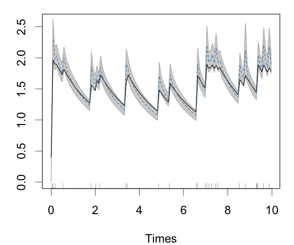
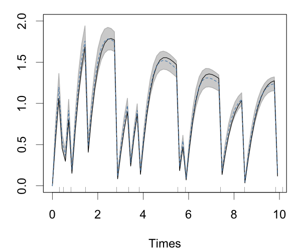
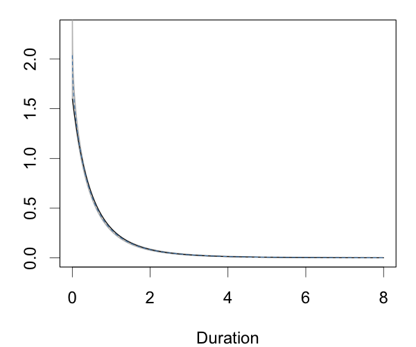
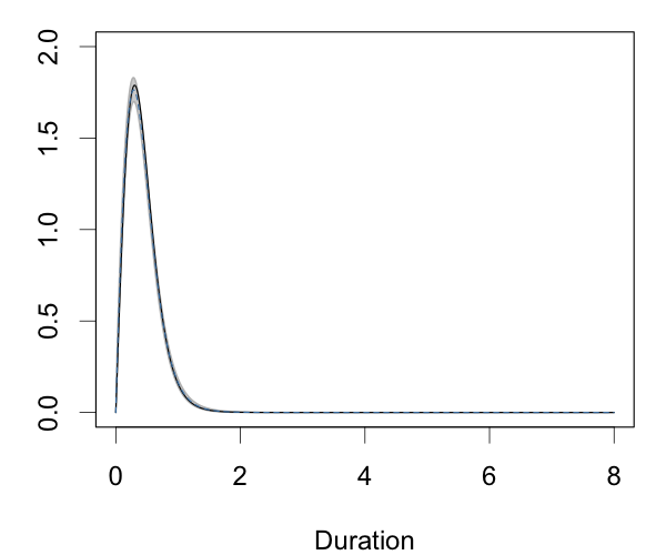
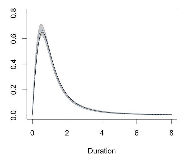
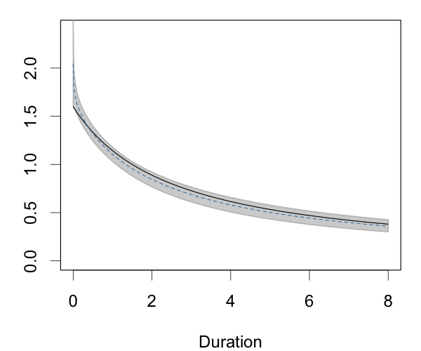
(a) scaled-Lomax

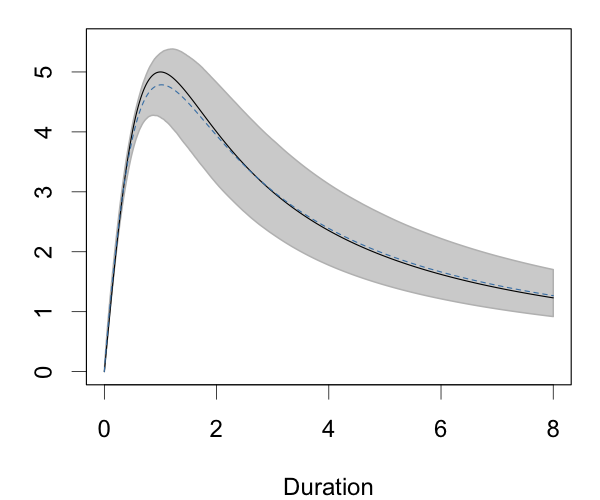
(b) Burr

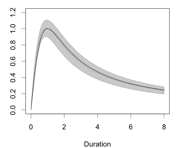
(c) Log-logistic

Figure 1: Synthetic data example. The first, second, and third rows plot posterior means (blue dashed lines) and $95\%$ credible interval estimates (grey bands) for the conditional intensity, marginal duration density, and marginal duration hazard function. The black solid lines correspond to the true functions.

We applied the Burr MTDPP model in (8), with $L=3$, to the three synthetic data sets. Recall that the hazard function of the marginal $\mathrm{Burr}(\gamma,\lambda,\kappa-1)$ duration distribution is decreasing when $\gamma\leq 1$, and hump-shaped when $\gamma>1$. We thus assigned a $\mathrm{Ga}(1,1)$ prior to $\gamma$, where $\mathrm{Ga}(a,b)$ denotes the gamma distribution with mean $a/b$. Moreover, the $m$th moment of the $\mathrm{Burr}(\gamma,\lambda,\kappa-1)$ distribution exists if $\gamma(\kappa-1)>m$. Independently of $\gamma$, we placed a truncated gamma prior, $\mathrm{Ga}(6,1)\mathbbm{1}(\kappa>1)$, on $\kappa$. Since $\text{E}(\kappa)=6.004$, the prior choice for $\gamma$ and $\kappa$ implies that, in prior expectation, the first five moments of the marginal duration distribution exist. The scale parameter $\lambda$ was assigned a $\mathrm{Ga}(1,1)$ prior, and the vector of weights a CDP$(5,1,2)$ prior.

Figure 1 plots point and interval estimates for the point process conditional intensity, as well as for the duration process marginal density and its associated hazard function. Note that, although the true data generating mechanisms correspond to MTDPPs, the Burr MTDPP is a mis-specified model for two of the simulated data sets. However, the model is able to distinguish between monotonic and non-monotonic hazard functions for the marginal duration distribution. Overall, based on a single process realization, the Burr MTDPP model provides reasonably accurate estimates for different point process functionals, with uncertainty bands that effectively contain the true functions.

4.2 IVT recurrence interval analysis

Integrated water vapor transport (IVT) is a vector representing the total amount of water vapor being transported in an atmospheric column. Atmospheric rivers (ARs), which are corridors of enhanced IVT, play a vital role in transporting moisture into western North America. Identifying and tracking ARs is central to understanding high-impact weather events, such as extreme precipitation and flooding. Rutz et al. (2019) review several of the AR detection algorithms, most of which use IVT thresholds as input. Appropriately thresholding the IVT is important to improve AR detection; e.g., Barata et al. (2022) provide a time-varying quantile estimate of the IVT using a dynamic statistical model.

In this example, we take on a different perspective to study the IVT, based on the general idea that strong ARs tend to associate with extreme IVT magnitudes. We obtain a collection of recurrent events for which the IVT magnitude exceeds a given threshold. Modeling extreme events using a point process approach is motivated by the asymptotic behavior of threshold exceedances. This approach assumes that, for a large threshold, the exccedances and the associated event times can be considered as a marked Poisson process (e.g., Kottas and Sansó 2007). On the other hand, the Poisson process assumption may be too restrictive, as well as unsuitable for applications where the inferential interest lies in the stationary distribution of the durations between event times. Studying the recurrence interval distribution is important in many areas, such as study of earthquakes above a certain magnitude (Corral, 2004) and extreme returns (Jiang et al., 2018). Depending on the correlation structure of the original time series, the recurrence interval distribution may exhibit different types of tail behavior (e.g., power law). Furthermore, the recurrence intervals can be dependent (Santhanam and Kantz, 2008). A generalization of the renewal process is needed in order to capture the dependence among durations.

Here, we demonstrate the potential of MTDPPs for the aforementioned goal, that is, simultaneously model the stationary recurrence interval distribution and capture the recurrence intervals dependence. Comparison between a renewal process model and the MTDPP model below shows that incorporating duration dependence improves prediction (results are included in the Supplementary Material).

The data set involves a time series of average daily IVT magnitude calculated using ERA5, a climate reanalysis that provides hourly estimates of atmospheric variables. The time series has 14965 observations, spanning from January 1, 1979 to December 31, 2019, with all February 29s omitted, corresponding to the Santa Cruz city in California. The data are publicly available in the R package exdqlm. Using the $0.95$ quantile threshold, we obtained 749 point events of IVT exceedances. The histogram of the durations (Figure 2(c)) suggests a heavy right tail for the recurrence interval distribution.

We consider the scaled-Lomax MTDPP. As previously discussed in Section 2.3, the model has a stationary scaled-Lomax marginal distribution $P(\alpha\phi,\alpha-1)$ for the recurrence intervals, and the conditional duration distribution converges to the exponential distribution with rate parameter $\phi^{-1}$, as $\alpha\rightarrow\infty$. Let $\{t_{i}\}$ and $\{x_{i}\}$ be the observed event times and durations, respectively. To account for potential seasonality, we use the following multiplicative model, $x_{i}=\mu(t_{i})z_{i}$, with $\log\mu(t_{i})=\sum_{j=1}^{J}\{\beta_{1j}\sin(j\omega t_{i})+\beta_{2j}\cos(j\omega t_{i})\},$ where $\omega=2\pi/T_{0}$, and $T_{0}=365$ is the period for daily data. We assume the stationary scaled-Lomax MTDPP model for the $z_{i}$, such that the conditional duration density is $f^{*}(x_{i})=$ $\mu(t_{i})^{-1}\sum_{l=1}^{L}w_{l}P\left(\mu(t_{i})^{-1}x_{i}\,|\,\alpha\phi+\mu(t_{i-l})^{-1}x_{i-l},\alpha\right)$. We took $J=5$, and assigned mean-zero, dispersed normal priors to the regression parameter vector. The shape and scale parameters $\alpha$ and $\phi$ received $\mathrm{Ga}(6,1)\mathbbm{1}(\alpha>1)$ and $\mathrm{Ga}(1,1)$ priors, respectively. We chose model order $L=15$; this was based on the ACF and PACF plots of the original data and the detrended data based on a harmonic regression, with a sensitivity analysis for $L$ (details can be found in the Supplementary Material). For the weights, we considered a $\mathrm{CDP}(5,1,6)$ prior, which implies a decreasing trend in prior expectation (Figure 2(e)).

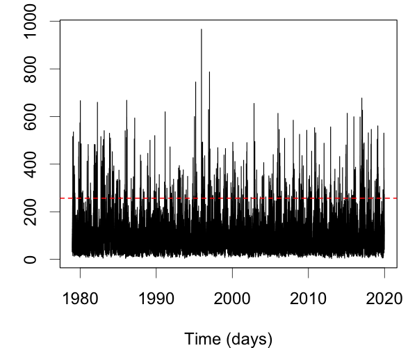
(a) Average daily IVT magnitude

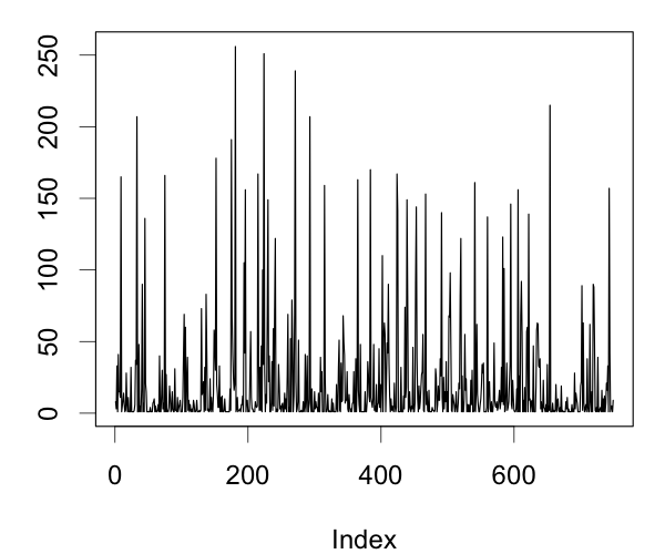
(b) Durations

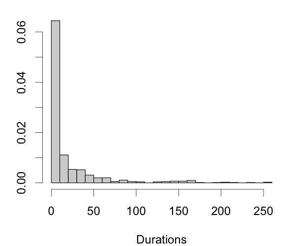
(c) Histogram of the durations

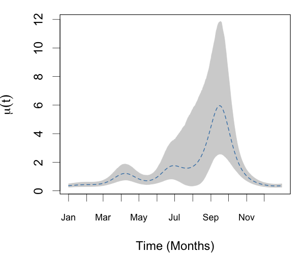
(d) Harmonic function $\mu(t)$

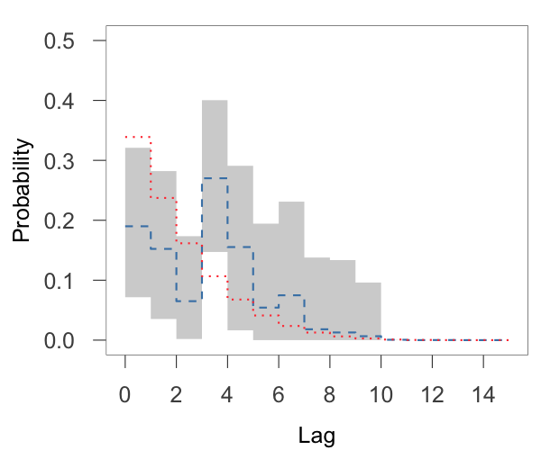
(e) Estimated weights

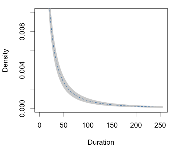
(f) Stationary marginal estimate

Figure 2: Recurrence interval analysis. Panel (a) shows the average daily IVT magnitude with the $0.95$ quantile (red line) fixed over time. Panels (b) and (c) plot the recurrence intervals and their histogram respectively. Panel (d) shows the harmonic function $\mu(t)$ for an one-year window. Panel (e) shows inference results for the weights. Panel (f) is the close view of the stationary marginal estimate, specifically at the tail of the marginal density. In Panels (d), (e), and (f), the blue dashed line and the light grey polygon correspond to the posterior mean and the pointwise $95\%$ credible interval estimates, respectively. The red dotted line in panel (e) is the prior mean.

We report the results based on the multiplicative model fitted to the original data. The posterior mean and $95\%$ credible interval estimates of the harmonic component coefficients imply the presence of annual and semiannual seasonality. The posterior estimates of the corresponding coefficients $(\beta_{11},\beta_{21},\beta_{22})$ are $-0.58\,(-0.86,-0.29)$, $-0.68\,(-1.06,-0.33)$, and $-0.53\,(-0.82,-0.23)$. Figure 2(d) shows the function $\mu(t)$ evaluated at a grid over a period of one year. Smaller durations between high IVT magnitudes tend to appear from November to March, corresponding to high atmospheric river frequency during that period. In fact, this time interval corresponds to the usual flooding period in California (e.g., the most recent floods in California were caused by multiple atmospheric rivers between December 2022 and March 2023). Figure 2(e) shows the estimated weights. Lags one, two, four and five are the most influential, which suggests serial dependence in the durations. The posterior mean and $95\%$ credible interval estimates of $\alpha$ and $\phi$ were $2.01\,(1.72,2.35)$ and $4.92\,(3.35,6.92)$, respectively. Note that the stationary marginal distribution of the process $\{z_{i}\}$ is $P(z\,|\,\alpha\phi,\alpha-1)$, with finite mean for $\alpha>2$ and finite variance for $\alpha>3$. Inference for $\alpha$ suggests that, even after adjusting for seasonality, the distribution of the recurrence intervals is heavy tailed. In fact, Figure 2(f) shows a marginal density tail that decays very slowly, in particular when compared to the histogram of the observed durations in Figure 2(c), where the seasonality is not accounted for. The heavy-tailed recurrence interval distribution also indicates a cluster phenomenon of the IVT extremes.

4.3 Mid-price changes of the AUD/USD exchange rate

Financial markets involve complex human activities, with both external and internal factors driving market dynamics. It is suggested that, for high-frequency financial data, price dynamics is more endogenous, driven largely by internal factors within the market itself (Filimonov and Sornette, 2012). Therefore, to understand financial market microstructure, it is important to quantify the level of endogeneity, measured as the proportion of price movements due to internal rather than external processes. Here, we explore modeling for endogeneity quantification from the duration clustering perspective using the MTDCPP, where each price move is considered as an event. At the end of the section, we discuss our findings relative to alternative models.

We analyze the price movements of the AUD/USD foreign exchange rate. A price movement is recorded when a mid-price change occurs, where mid-price is defined as the average of the best bid and ask prices (Filimonov and Sornette, 2012). The data set consists of 121 non-overlapping point patterns, with total number of events ranging from 108 to 3961. Each point pattern corresponds to an one-hour time window of the trading week from 20:00 Greenwich Mean Time (GMT) July 19 to 21:00 GMT July 24 in 2015. Analyzing sequences of point patterns within small time windows avoids to some extent the issue of nonstationarity, such as diurnal pattern. We refer to Chen and Stindl (2018) for more details about the data, which are available in R package RHawkes (Chen and Stindl, 2022).

We considered the Lomax MTDCPP, that is, model (9) with $f_{I}$ given by an exponential density with rate parameter $\mu$, and $f^{*}$ corresponding to the stationary Lomax MTDPP. In particular, the self-exciting Lomax MTDPP is regarded as the driver of internal factors, such as market participants’ anticipations and reactions to market prices. In contrast, external information is driven by the exponential density, which is independent of the past durations. Thus, the probability $(1-\pi_{0})$ corresponding to the Lomax MTDPP can be interpreted as the proportion of price movements due to endogenous interactions.

We applied the model to each of the 121 point patterns and, for illustrative purposes, considered the same model specification for all point patterns. Based on previous studies on market endogeneity, we used a $\mathrm{Beta}(5,5)$ prior for $\pi_{0}$. The prior assigns small probabilities to values of $\pi_{0}$ around $0$ or $1$, which correspond to the less likely scenarios where the market is driven by only an internal or an external process. For component-density parameters, we used a $\mathrm{Ga}(1,1)$ prior for $\mu$, and $\mathrm{Ga}(\alpha\,|\,6,1)\mathbbm{1}(\alpha>1)$ and $\mathrm{Ga}(\phi\,|\,1,1)$ priors for the shape and scale parameter of the Lomax model, respectively. Based on the PACF of the observed durations (see the Supplementary Material for details), we chose model order $L=15$ for all point patterns, and the mixture weights were assigned a CDP$(5,1,6)$ prior.

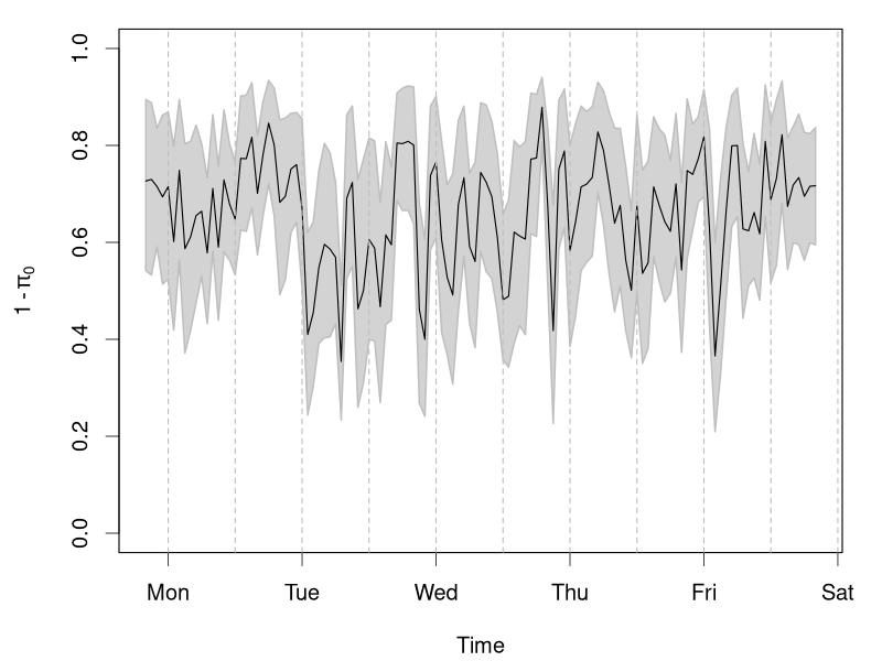
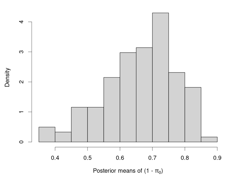
Figure 3: AUD/USD foreign exchange market endogeneity analysis. Left panel: Time series of the posterior means (solid lines) and pointwise $95\%$ credible intervals (grey polygons) for the level of endogeneity $1-\pi_{0}$. Vertical dashed lines correspond to midnight and midday GMT. Right panel: Histogram of the posterior means of $1-\pi_{0}$ for the $121$ one-hour time windows.

We focus on inference for the level of endogeneity $(1-\pi_{0})$; additional results are available in the Supplementary Material. The time series of posterior means and interval estimates of $(1-\pi_{0})$ (for the $121$ one-hour time windows) shows that the level of endogeneity fluctuated heavily over the trading week (Figure 3, left panel). The histogram of the posterior means is skewed to the left (Figure 3, right panel), with median $0.68$ and quartiles $(0.59,0.74)$, suggesting that the market dynamics were mostly driven by internal processes.

A similar conclusion was drawn by Chen and Stindl (2018), where a renewal Hawkes process (RHawkes; Wheatley et al. 2016) was applied to the same data; the mean and quartiles of their estimates for the level of endogeneity over the trading week were, respectively, $0.66$ and $(0.53,0.80)$. The RHawkes process extends the Hawkes process to capture dependence between clusters, by replacing the immigrant Poisson process with a renewal process. Both the Hawkes and RHawkes process models include a branching ratio parameter, which can be used to quantify the level of endogeneity (Filimonov and Sornette, 2012; Wheatley et al., 2016; Chen and Stindl, 2018). Under a different stochastic model structure, the Lomax MTDCPP is able to quantify the extent to which the observed dynamics are caused by internal factors versus external influences.

We note that using the MTDCPP for the present example does not require any stationarity assumptions. In contrast, stationarity is essential for both the Hawkes and RHawkes processes in order to use the branching ratio as an estimator for the level of endogeneity. However, as discussed in Filimonov and Sornette (2012), market activities are commonly nonstationary. The lack of stationarity is typically attributed to seasonal trends, which can be addressed by splitting the time window into small intervals, as shown in this example. Still, one has to balance the size of the intervals and the number of the events within the interval to ensure reliable estimates are produced. Moreover, even after removing seasonality, stationarity is not necessarily guaranteed. Therefore, MTDCPP models may be useful in applications where stationarity assumptions are not plausible.

5 Summary and discussion

We have developed a new class of stochastic models for temporal point patterns with self-excitation or self-regulation effects, identically distributed but dependent durations, or clustered durations. The modeling framework allows for different approaches to building the point process: through marginal duration distributions, when the inferential goal pertains to the intervals between event times; or through conditional hazard functions, when interest lies in the point process dependence structure on its history. Both strategies connect naturally to existing point process models. The former is analogous to renewal process modeling, while the latter involves the same motivation of Hawkes processes. We have prsented several examples of implementing these strategies. The Burr model, which allows for point process functionals with flexible shapes, can be considered as a default choice for general purposes, while the scaled-Lomax model, which provides flexible tail behavior, may be considered for scientific applications where such property is relevant.

Our framework builds from a structured mixture model for the point process conditional duration density. The resulting point process has restricted memory, i.e., its evolution depends on recent events. This assumption is generally suitable for relatively large point patterns. For scenarios where one anticipates more extensive history dependence, a large value for the order of the mixture model can be used. The nonparametric prior for the weights allows efficient inference with a large order. On the other hand, there are applications where data correspond to many processes that exhibit a relatively small number of point events, such as the analysis of recurrent event gap times for multiple patients in medical studies. For such data, a small order is more appropriate. In fact, even the special case where the conditional duration density depends on the most recent lag provides a meaningful generalization of renewal processes commonly used for this type of analysis.

In many applications, point patterns include information on marks, that is, random variables associated with each point event, such that the data generating mechanism corresponds to a marked point process. Consider, for instance, continuous marks, $\bm{y}$. The marked point process intensity can be developed from $\lambda^{*}(t,\bm{y})=$ $\lambda_{g}^{*}(t)\,m^{*}_{t}(\bm{y})$, where $\lambda_{g}^{*}(t)$ is the conditional intensity for the event times (referred to as the ground process intensity), and $m^{*}_{t}(\bm{y})$ is the time-dependent mark distribution (Daley and Vere-Jones, 2003). The proposed framework can be utilized for marked point processes by combining an MTDPP or MTDCPP model for the ground process with a model for the mark distribution.

Supplementary Material

The Supplementary Material includes proofs for the theoretical results, details for the bivariate Burr distribution, additional details for the MCMC algorithms and predictions, additional data examples and results, MCMC diagnostics, and model checking results.

Supplementary Material for “Mixture Modeling for Temporal Point Processes with Memory”

S1 Theoretical results

S1.1 Proofs of theorem and propositions

Proof of Theorem 1.

Consider a stationary MTD point process, that is, the corresponding duration process $\{X_{i}:i\geq 1\}$ has a stationary marginal distribution. Thus, the durations $X_{1},\dots,X_{N(t)}$ are a collection of dependent random variables that are identically distributed. We assume that the first and second moments with respect to the stationary marginal distribution exist and are finite.

Denote by $E(X_{i})=\mu$ for all $i$. Let $T_{N(t)}=\sum_{i=1}^{N(t)}X_{i}$ be the last arrival time prior to $t$ or the arrival time at $t$. For $N(t)\geq 1$, We have that $T_{N(t)}\leq t<T_{N(t)+1}$, and that $T_{N(t)}/N(t)<t/N(t)<T_{N(t)+1}/N(t)$. Note that $T_{N(t)}/N(t)$ is the average of the durations $X_{1},\dots,X_{N(t)}$. By the strong law of large numbers for dependent non-negative random variables korchevsky2010strong, we have that, as $t\rightarrow\infty$, $T_{N(t)}/N(t)\rightarrow\mu\;a.s.$, since as $t\rightarrow\infty$, $N(t)\rightarrow\infty$. Observing that $T_{N(t)+1}/N(t)=\{T_{N(t)+1}/(N(t)+1)\}\{(N(t)+1)/N(t)\}$, where the first term $T_{N(t)+1}/(N(t)+1)\rightarrow\mu\;a.s.$, and the second term $(N(t)+1)/N(t)\rightarrow 1$, we can conclude that $N(t)/t\rightarrow 1/\mu\;a.s.$. ∎

Proof of Proposition 1.

Let $X_{i}$ be the duration associated with event time $t_{i}$. By Definition 1 in the main paper, the conditional density of $X_{i}$ is $f^{*}(x_{i})\equiv f^{*}(t_{i}-t_{i-1})=f^{*}(t_{i}-t_{N(t_{i}^{-})})$, where $x_{i}=t_{i}-t_{i-1}$, for $i\geq 2$. Then, according to (3) and (4) in the main paper, we have that $f^{*}(x_{i})=\sum_{l=1}^{i-2}w_{l}\,f_{l}(x_{i}\,|\,x_{i-l})+(1-\sum_{r=1}^{i-2}w_{r})f_{i-1}(x_{i}\,|\,x_{1}),\;i=2,\dots,L$, and $f^{*}(x_{i})=\sum_{l=1}^{L}w_{l}\,f_{l}(x_{i}\,|\,x_{i-l}),\;i>L$.

Let $f_{X}$ be a marginal density of interest, and denote by $g_{i}(x_{i})$ the marginal density of $X_{i}$, for $i\geq 1$. By condition (i) in Proposition 1, we have that $g_{1}(x_{1})\equiv f_{X}(x_{1})$. Then using both conditions (i) and (ii) in the proposition, we can show that for $i\geq 2$,

$$g_{i}(x_{i})=\int f^{*}(x_{i})\,p(x_{1},\dots,x_{i-1})\,dx_{1},\dots,dx_{i-1}=f_{X}(x_{i}),$$ (1)

where $p(x_{1})\equiv g_{1}(x)$ and $p(x_{1},\dots,x_{i-1})$ is the joint density for random vector $(X_{1},\dots,X_{i-1})$, for $i\geq 3$. The second equality in (1) follows the approach in Zheng et al. (2022).

∎

Proof of Proposition 2.

The definition of the conditional intensity function $\lambda^{*}(t)$ yields that $m(t)=E[N(t)]=E[\int_{0}^{t}\lambda^{*}(u)du]$, where the expectation is taken with respect to the probability distribution of the point process. Since our interest is in $\lim_{t\rightarrow\infty}m(t)/t$, consider time $t$ large enough such that $N(t)\geq L$.

Recall that $\lambda^{*}(t)\equiv h^{*}(t-t_{N(t^{-})})=f^{*}(t-t_{N(t^{-})})/S^{*}(t-t_{N(t^{-})})$, where $h^{*}(t-t_{N(t^{-})})$ and $S^{*}(t-t_{N(t^{-})})$ are the hazard and survival functions, respectively, associated with $f^{*}(t-t_{N(t^{-})})$. Let $t_{0}=0$. We have that

$$\int_{0}^{t}\lambda^{*}(u)du =\sum_{i=1}^{N(t^{-})}\int_{t_{i-1}}^{t_{i}}h^{*}(u-t_{i-1})du+\int_{t_{N(t^{-})}}^{t}h^{*}(u-t_{N(t^{-})})du$$ (2)

$$=\sum_{i=1}^{N(t^{-})}(-\log\{S^{*}(t_{i}-t_{i-1})\})-\log\{S^{*}(t-t_{N(t^{-})})\}.$$

For $i=1,\dots,N(t^{-})$, by Jensen’s inequality, we have that

$$-\log\{S^{*}(t_{i}-t_{i-1})\} =-\log\left\{\sum_{l=1}^{L}w_{l}S_{l}(t_{i}-t_{i-1}\,|\,t_{i-l}-t_{i-1-l})\right\}$$ (3)

$$\leq\sum_{l=1}^{L}w_{l}\left(-\log\{S_{l}(t_{i}-t_{i-1}\,|\,t_{i-l}-t_{i-1-l})\}\right)$$

$$=\sum_{l=1}^{L}w_{l}\int_{t_{i-1}}^{t_{i}}h_{l}(u-t_{i-1}\,|\,t_{i-l}-t_{i-1-l})du=\tilde{\Lambda}^{*}(t_{i}-t_{i-1}),$$

where $\tilde{\Lambda}^{*}(a-t_{k})=\sum_{l=1}^{L}w_{l}\int_{t_{k}}^{a}h_{l}(u-t_{k}\,|\,t_{k-l+1}-t_{k-l})du$. Similarly, applying Jensen’s inequality, we obtain $-\log\{S^{*}(t-t_{N(t^{-})})\}\leq\tilde{\Lambda}^{*}(t-t_{N(t^{-})})$, and combining (2) and (3), we have that $\int_{0}^{t}\lambda^{*}(u)du\,\leq\,\sum_{i=1}^{N(t^{-})}\tilde{\Lambda}^{*}(t_{i}-t_{i-1})\,+\,\tilde{\Lambda}^{*}(t-t_{N(t^{-})}).$

If $h_{l}\leq B_{l}$ for all $l$, then $\tilde{\Lambda}^{*}(t_{i}-t_{i-1})\leq\sum_{l=1}^{L}w_{l}(t_{i}-t_{i-1})B_{l}$, for $i=1,\dots,N(t^{-})$, and $\tilde{\Lambda}^{*}(t-t_{N(t^{-})})\leq\sum_{l=1}^{L}w_{l}(t-t_{N(t^{-})})B_{l}$. Then we have that

$$\int_{0}^{t}\lambda^{*}(u)du \leq\,\sum_{i=1}^{N(t^{-})}\sum_{l=1}^{L}w_{l}(t_{i}-t_{i-1})B_{l}+\sum_{l=1}^{L}w_{l}(t-t_{N(t^{-})})B_{l}$$

$$=t_{N(t^{-})}\sum_{l=1}^{L}w_{l}B_{l}+(t-t_{N(t^{-})})\sum_{l=1}^{L}w_{l}B_{l}=t\sum_{l=1}^{L}w_{l}B_{l}.$$

Hence, the function $m(t)\leq t\sum_{l=1}^{L}w_{l}B_{l}$. It follows that $\lim_{t\rightarrow\infty}m(t)/t\leq\sum_{l=1}^{L}w_{l}B_{l}$. ∎

Proof of Proposition 3.

Let $(U,V)=(\alpha X,\alpha Y)$, where the joint density of $(X,Y)$ is $f_{X,Y}(x,y)\propto(\lambda_{0}+\lambda_{1}x+\lambda_{2}y)^{-(\alpha+1)}$, which corresponds to the bivariate Lomax distribution of Arnold et al. (1999). By change of variable, we obtain the joint density of $(U,V)$, namely, $f_{U,V}(u,v)\propto(\lambda_{0}a+\lambda_{1}u/\alpha+\lambda_{2}v/\alpha)^{-(\alpha+1)}$, with normalizing constant $C=\int_{0}^{\infty}\int_{0}^{\infty}(\lambda_{0}+\lambda_{1}u/\alpha+\lambda_{2}v/\alpha)^{-(\alpha+1)}dudv=\alpha\lambda_{0}^{-(\alpha-1)}\{(\alpha-1)\lambda_{1}\lambda_{2}\}^{-1}$. The marginal density of $U$ is

$$f_{U}(u) =C^{-1}\int_{0}^{\infty}\alpha^{-2}(\lambda_{0}+\lambda_{1}u/\alpha+\lambda_{2}v/\alpha)^{-(\alpha+1)}dv$$

$$=(\alpha-1)(\lambda_{0}\alpha)^{-1}\lambda_{1}\{1+(\lambda_{0}\alpha)^{-1}\lambda_{1}u\}^{-\alpha}.$$

Since $u$ and $v$ are symmetric in the joint density $f_{U,V}(u,v)$, the marginal density $f_{V}(v)=(\alpha-1)(\lambda_{0}\alpha)^{-1}\lambda_{2}\{1+(\lambda_{0}\alpha)^{-1}\lambda_{2}v\}^{-\alpha}$. It follows that $f_{U|V}(u\,|\,v)=f_{U,V}(u,v)/f_{V}(v)=\alpha\lambda_{1}(\alpha\lambda_{0}+\lambda_{2}v)^{-1}\{1+\lambda_{1}u(\alpha\lambda_{0}+\lambda_{2}v)^{-1}\}^{-(\alpha+1)}$. Similarly, we have that $f_{V|U}(v\,|\,u)=f_{U,V}(u,v)/f_{U}(u)=\alpha\lambda_{2}(\alpha\lambda_{0}+\lambda_{1}u)^{-1}\{1+\lambda_{2}v(\alpha\lambda_{0}+\lambda_{1}u)^{-1}\}^{-(\alpha+1)}$. ∎

Proof of Proposition 4.

Consider the stationary scaled-Lomax MTDPP with marginal duration density $P(\alpha\phi,\alpha-1)$. Suppose $N(t)\geq 1$. The survival function of the conditional duration distribution can be expressed as

$$S^{*}(t-t_{N(t^{-})})=\sum_{l=1}^{t_{L}}w_{l}^{*}\,\left(1+\frac{t-t_{N(t^{-})}}{\alpha\phi+t_{N(t^{-})-l+1}-t_{N(t^{-})-l}}\right)^{-\alpha},$$

where $t_{L}=\min\{N(t^{-}),L\}$. In particular, for $N(t^{-})\geq L$, $w_{l}^{*}=w_{l}$, for $l=1,\dots,L$. When $1\leq N(t^{-})<L$, $w_{l}^{*}=1,\dots,t_{L}-1$, and $w_{t_{L}}^{*}=1-\sum_{r=1}^{t_{L}-1}w_{r}$. It follows that the weights $w_{l}^{*}$ satisfy $\sum_{l=1}^{t_{L}}w_{l}^{*}=1$ for $N(t)\geq 1$.

Then, for $N(t)\geq 1$, we have that

$$S^{*}(t-t_{N(t^{-})}) =\sum_{l=1}^{t_{L}}w_{l}^{*}\left\{\left(1+\frac{t-t_{N(t^{-})}}{\alpha\phi+t_{N(t^{-})-l+1}-t_{N(t^{-})-l}}\right)^{-(\alpha\phi+t_{N(t^{-})-l+1}-t_{N(t^{-})-l})}\right\}^{1/\phi}$$ (4)

$$\;\;\;\;\;\;\;\;\;\;\;\;\times\left(1+\frac{t-t_{N(t^{-})}}{\alpha\phi+t_{N(t^{-})-l+1}-t_{N(t^{-})-l}}\right)^{(t_{N(t^{-})-l+1}-t_{N(t^{-})-l})/\phi}.$$

As $\alpha\rightarrow\infty$, the limits of the first term and the second term in the $l$th mixture component of (4) are $\exp(-(t-t_{N(t^{-})})\phi^{-1})$ and $1$, respectively. More specifically, the limit of the first term is obtained by using the results that (i) $\lim_{n\rightarrow\infty}(1+x/n)^{n}=\exp(x)$; (ii) $\lim_{n\rightarrow\infty}g_{1}(n)/g_{2}(n)=\lim_{n\rightarrow\infty}g_{1}(n)/\lim_{n\rightarrow\infty}g_{2}(n)$, provided that both $\lim_{n\rightarrow\infty}g_{1}(n)$ and $\lim_{n\rightarrow\infty}g_{2}(n)$ exist, and $\lim_{n\rightarrow\infty}g_{2}(n)\neq 0$.

Since $\sum_{l=1}^{t_{L}}w_{l}^{*}=1$, it follows that, as $\alpha\rightarrow\infty$, the survival function of the conditional duration distribution converges to $\exp(-(t-t_{N(t^{-})})\phi^{-1})$, which is the survival function of an exponential distribution with rate parameter $\phi^{-1}$.

∎

S1.2 Identifiability

Identifiability of a standard finite mixture model, commonly referred to as generic identifiability (e.g., fruhwirth2006finite), has been well addressed in the literature (see, e.g., teicher1961identifiability,teicher1963identifiability,yakowitz1968identifiability,chandra1977mixtures,kent1983identifiability,crawford1994application). Generally, a regular finite mixture model is said to be identifiable if no two sets of parameter values, up to permutation of the components, produce the same distribution or density mclachlan2019finite. We refer to Chapter 3 in titterington1985statistical for a detailed discussion of the generic identifiability and relevant theoretical results.

We present below a definition of the identifiability for MTDPPs.

Definition S3.

Given a realization of durations, $(x_{1},\dots,x_{n})$, consider an MTDPP model with conditional duration density given in (4) of the main paper, with parameters $\{\bm{w},\bm{\theta}\}\in\bm{\Psi}$, the associated parameter space, where $\bm{w}=(w_{1},\dots,w_{L})^{\top}$ is the vector of weights and $\bm{\theta}=\{\bm{\theta}_{1},\dots,\bm{\theta}_{L}\}$ denotes the component parameters. The MTDPP is said to be identifiable if for any two sets of parameters $\{\bm{w},\bm{\theta}\},\{\bm{w}^{\prime},\bm{\theta}^{\prime}\}\in\bm{\Psi}$,

$$\sum_{l=1}^{L}w_{l}f_{l}(x_{i}\,|\,x_{i-l},\bm{\theta}_{l})=\sum_{l=1}^{L^{\prime}}w_{l}^{\prime}f_{l}(x_{i}\,|\,x_{i-l},\bm{\theta}^{\prime}_{l})$$ (5)

for each $i=L+1,\dots,n$ and for all possible values of $x_{i}$, implies that $L=L^{\prime}$, $w_{l}=w_{l}^{\prime}$, and $\bm{\theta}_{l}=\bm{\theta}^{\prime}_{l}$, $l=1,\dots,L$.

Definition S3 suggests that we can use established results for standard finite mixture models to verify the identifiability of an MTDPP, by treating the conditional density in (5) for each $i$ as a standard finite mixture model. A similar idea has been used in Hassan and Lii (2006) to verify the identifiability of their proposed bivariate MTD models. As examples, we demonstrate the identifiability of the Burr MTDPP, the Lomax MTDPP, and the scaled-Lomax MTDPP, which are illustrated in Section 2.3 of the main paper.

Burr MTDPP

To verify the identifiability of the class of Burr MTDPPs, it suffices to show that a finite mixture of the corresponding Burr distributions is identifiable. Identifiability for finite mixtures of Burr distributions has been studied in ahmad1994small and al2016mixture. In particular, ahmad1994small shows that, for the two-parameter Burr-Type-VII distribution with c.d.f. $F(x)=1-(1+x^{\gamma})^{-\kappa}$, the corresponding finite mixture model is identifiable with a common shape parameter $\gamma$, using Theorem 1 in teicher1963identifiability. More recently, al2016mixture shows that the finite mixtures of two-parameter Burr-Type-III distributions with c.d.f. $F(x)=(1+x^{-\gamma})^{-\kappa}$ is identifiable, using Theorem 2.4 in chandra1977mixtures.

Here, we show that the finite mixtures of three-parameter Burr-Type-VII distributions with c.d.f. $F(x)=1-(1+(x/\lambda)^{\gamma})^{-\kappa}$ is identifiable, using Theorem 2.4 in chandra1977mixtures.

Proof.

Let $\mathcal{F}=\{F(x;\kappa,\gamma,\lambda)=1-(1+(x/\lambda)^{\gamma})^{-\kappa};\kappa>0,\gamma>0,\lambda>0\}$ be the family of three-parameter Burr-Type-VII distributions. Consider the following transformation,

$$\phi_{i}(t)=E(X^{t})=\lambda_{i}^{-t}\kappa_{i}\,B(\kappa_{i}-t/\gamma_{i},1+t/\gamma_{i}),\;t<\kappa_{i}\gamma_{i},$$

where $B(a,b)=\Gamma(a)\Gamma(b)/\Gamma(a+b)$ is the beta function, and $E(X^{t})$, for a random variable $X$, is taken with respect to a Burr distribution with c.d.f. $F_{i}(x)\in\mathcal{F}$, where $F_{i}(x)\equiv F(x;\kappa_{i},\gamma_{i},\lambda_{i})=1-(1+(x/\lambda_{i})^{\gamma_{i}})^{-\kappa_{i}}$.

We order the family lexicographically by: $F_{1}(x)<F_{2}(x)$ if $\kappa_{1}<\kappa_{2}$, or if $\kappa_{1}=\kappa_{2}$ but $\gamma_{1}<\gamma_{2}$, or if $\kappa_{1}=\kappa_{2},\gamma_{1}=\gamma_{2}$ but $\lambda_{1}>\lambda_{2}$. Then we have that $D_{\kappa_{1}\gamma_{1}}\subseteq D_{\kappa_{2}\gamma_{2}}$, where $D_{\kappa_{i}\gamma_{i}}=(-\infty,\kappa_{i}\gamma_{i})$, $i=1,2$. Take $t_{1}=\kappa_{1}\gamma_{1}$ and note that $t_{1}$ in the closure of $D_{\kappa_{1}\gamma_{1}}$. Then we have that

$$\lim_{t\rightarrow t_{1}}\phi_{1}(t) =\lim_{t\rightarrow\kappa_{1}\gamma_{1}}\lambda_{1}^{-t}\kappa_{1}B(\kappa_{1}-t/\gamma_{1},1+t/\gamma_{1})$$

$$=\lim_{t\rightarrow\kappa_{1}\gamma_{1}}\lambda_{1}^{-t}\,\Gamma(\kappa_{1}-t/\gamma_{1})\,\Gamma(1+t/\gamma_{1})=\infty,$$

since $\lim_{t\rightarrow\kappa_{1}\gamma_{1}}\Gamma(\kappa_{1}-t/\gamma_{1})=\infty$, $\lim_{t\rightarrow\kappa_{1}\gamma_{1}}\lambda_{1}^{-t}=\lambda_{1}^{-\kappa_{1}\gamma_{1}}$, and $\lim_{t\rightarrow\kappa_{1}\gamma_{1}}\Gamma(1+t/\gamma_{1})=\Gamma(1+\kappa_{1})>0$. On the other hand, we have that

$$\lim_{t\rightarrow t_{1}}\phi_{2}(t) =\lim_{t\rightarrow\kappa_{1}\gamma_{1}}\lambda_{1}^{-t}\kappa_{2}\,B(\kappa_{2}-t/\gamma_{2},1+t/\gamma_{2})$$

$$=\lambda_{1}^{-\kappa_{1}\gamma_{1}}\,\Gamma(\kappa_{2}-\kappa_{1}\gamma_{1}/\gamma_{2})\,\Gamma(1+\kappa_{1}\gamma_{1}/\gamma_{2})>0.$$

It follows that $\lim_{t\rightarrow t_{1}}\phi_{2}(t)/\phi_{1}(t)=0$ and Theorem 2.4 of chandra1977mixtures applies. ∎

Since a finite mixture of three-parameter Burr-Type-VII distributions is identifiable, based on Definition S3, we have that $L=L^{\prime}$, $w_{l}=w^{\prime}_{l}$, $\kappa=\kappa^{\prime}$, $\gamma=\gamma^{\prime}$, and $(\lambda^{\gamma}+x_{i-l}^{\gamma})^{1/\gamma}=(\lambda^{\prime\gamma^{\prime}}+x_{i-l}^{\gamma^{\prime}})^{1/\gamma^{\prime}}$, for each $l$ and for each $i$. It follows that $\lambda=\lambda^{\prime}$ for each $i$. Thus, the class of Burr MTDPPs is identifiable based on Definition S3.

Lomax and Scaled-Lomax MTDPPs

The scaled-Lomax distribution can be treated as a reparameterized Lomax distribution, and thus it suffices to prove the identifiability for the Lomax MTDPP. Note that ahmad1988identifiability has verified that a finite mixture of Pareto-Type-I distributions is identifiable. Note that the Lomax distribution is a shifted version of the Pareto-Type-I distribution. Specifically, for a Pareto-Type-I distribution with c.d.f. $F(x)=1-(x/\lambda)^{-\alpha}$, the c.d.f. of the corresponding Lomax distribution is $F(x)=1-((x+\lambda)/\lambda)^{-\alpha}=1-(1+x/\lambda)^{-\alpha}$. It follows that a finite mixture of Lomax distributions is identifiable. Based on Definition S3, we have that $L=L^{\prime}$, $w_{l}=w^{\prime}_{l}$, $\alpha_{l}=\alpha^{\prime}_{l}$, and $\phi_{l}+x_{i-l}=\phi_{l}^{\prime}+x_{i-l}$, for each $l$ and for each $i$. It follows that $\phi_{l}=\phi^{\prime}_{l}$ for each $l$ and for each $i$. Thus, the class of Lomax MTDPPs is identifiable, and so is the class of scaled-Lomax MTDPPs.

S2 Bivariate Burr distribution

Let $X$ be a random variable, and its cumulative distribution function (c.d.f.) is $F(x)=1-\left(1+(x/\lambda)^{\gamma}\right)^{-\psi}$. We say that $X$ follows a three-parameter Burr distribution tadikamalla1980look, denoted as $\mathrm{Burr}(x\,|\,\gamma,\lambda,\psi)$. We will use such notation throughout to indicate either the distribution or its density for a Burr random variable, depending on the context (we follow the same notation approach for other distributions).

Consider a bivariate random vector $(X,Y)$, with marginal c.d.f.s for $X$ and $Y$ given by $F(x)=1-\left(1+(x/\lambda)^{\gamma}\right)^{-\psi}$ and $F(y)=1-\left(1+(y/\lambda)^{\gamma}\right)^{-\psi}$, respectively. The joint c.d.f. $F(x,y)$ is specified by the heavy right tail (HRT) copula given by

$$C(u,v)=u+v-1+\left[(1-u)^{-1/a}+(1-v)^{-1/a}-1\right]^{-a},$$ (6)

where $0\leq u\leq 1$, $0\leq v\leq 1$, and $a>0$ frees1998understanding.

We set the copula parameter to be the same as the second shape parameter of the Burr distribution, that is, $a=\psi$. Replace $u$ and $v$ with $F(x)$ and $F(y)$, respectively, in (6). Then, the joint c.d.f. of the random vector $(X,Y)$ is given by

$$F(x,y) =F(x)+F(y)-1+\left[(1-F(x))^{-1/\psi}+(1-F(y))^{-1/\psi}-1\right]^{-\psi}$$

$$=1-\left(1+\left(\frac{x}{\lambda}\right)^{\gamma}\right)^{-\psi}-\left(1+\left(\frac{y}{\lambda}\right)^{\gamma}\right)^{-\psi}+\left[1+\left(\frac{x}{\lambda}\right)^{\gamma}+\left(\frac{y}{\lambda}\right)^{\gamma}\right]^{-\psi}.$$

The conditional c.d.f. of $Y$ given $X=x$ is $F(y\,|\,x)=\partial C(F(x),F(y))/\partial F(x)$. Note that $\partial C(u,v)/\partial u=1-\left[(1-u)^{-1/\psi}\right]^{\psi+1}\left[(1-u)^{-1/\psi}+(1-v)^{-1/\psi}-1\right]^{-(\psi+1)}$. It follows that

$$F(y\,|\,x) =1-\left[1+\left(\frac{x}{\lambda}\right)^{\gamma}\right]^{\psi+1}\left[1+\left(\frac{x}{\lambda}\right)^{\gamma}+1+\left(\frac{y}{\lambda}\right)^{\gamma}-1\right]^{-(\psi+1)}$$ (7)

$$=1-\left[1+\frac{\left(\frac{y}{\lambda}\right)^{\gamma}}{1+\left(\frac{x}{\lambda}\right)^{\gamma}}\right]^{-(\psi+1)}=1-\left[1+\frac{y^{\gamma}}{\lambda^{\gamma}+x^{\gamma}}\right]^{-(\psi+1)}$$

$$=1-\left[1+\left(\frac{y}{\tilde{\lambda}(x)}\right)^{\gamma}\right]^{-(\psi+1)},$$

where $\tilde{\lambda}(x)=(\lambda^{\gamma}+x^{\gamma})^{1/\gamma}$. Therefore, the conditional distribution of $Y$ given $X=x$ is a Burr distribution, $\mathrm{Burr}(\gamma,\tilde{\lambda}(x),\psi+1)$. Since the HRT copula is symmetric in its arguments, the conditional distribution of $X$ given $Y=y$ is also a Burr distribution.

We note that the bivariate Burr distribution defined through the HRT copula and Burr marginals was considered in venter2002tails. However, the expressions for the conditional c.d.f.s reported in venter2002tails include an error. Equation (7) provides the corrected expression for the conditional c.d.f. of $Y$ given $X$.

S3 Additional details for Bayesian implementation

In Section S3.1, we provide details for posterior prediction using MTDPPs. Posterior inference and prediction for MTDCPPs are introduced in Section S3.2.

The observed point pattern comprises event times $0=t_{0}<t_{1}<\ldots<t_{n}<T$, with corresponding observed durations $x_{i}=t_{i}-t_{i-1}>0$, for $i=1,\dots,n$. Let $D_{n}=\{t_{1},\dots,t_{n},t_{n+1}>T\}$, for $n>L$, represent the information from the observed point pattern. Note that, as its description highlights, $D_{n}$ includes the information that the (unobserved) event time $t_{n+1}$ is greater than the upper bound $T$ of the time observation window, i.e., that the (unobserved) duration $x_{n+1}$ is greater than $T-t_{n}$.

S3.1 Posterior prediction for MTDPPs

To obtain the posterior predictive density for the next duration, $p(x_{n+1}\,|\,D_{n})$, we first derive the conditional density for the next duration given the model parameters, $\{\bm{\theta},\bm{w}\}$, and $D_{n}$. As discussed above, $D_{n}$ implies conditioning on event $x_{n+1}>T-t_{n}$. Therefore, using Equation (4) in the main paper, we obtain:

$$p(x_{n+1}\,|\,D_{n},\bm{\theta},\bm{w}) =f^{*}(x_{n+1})\,/\,S^{*}(T-t_{n})$$ (8)

$$=\frac{\sum_{l=1}^{L}w_{l}\,f_{l}(x_{n+1}\,|\,x_{n+1-l},\bm{\theta}_{l})}{\int_{T-t_{n}}^{\infty}\sum_{l=1}^{L}w_{l}\,f_{l}(x_{n+1}\,|\,x_{n+1-l},\bm{\theta}_{l})\,dx_{n+1}}$$

$$=\frac{\sum_{l=1}^{L}w_{l}\,S_{l}(T-t_{n}\,|\,x_{n+1-l},\bm{\theta}_{l})\,\tilde{f}_{l}(x_{n+1}\,|\,x_{n+1-l},\bm{\theta}_{l})}{\sum_{l=1}^{L}w_{l}\,S_{l}(T-t_{n}\,|\,x_{n+1-l},\bm{\theta}_{l})}$$

$$=\sum_{l=1}^{L}w_{l}^{*}(T)\,\tilde{f}_{l}(x_{n+1}\,|\,x_{n+1-l},\bm{\theta}_{l}),\,\,\,\,\,x_{n+1}\in(T-t_{n},\infty).$$

Here, the weights $w_{l}^{*}(T)=w_{l}\,S_{l}(T-t_{n}\,|\,x_{n+1-l},\bm{\theta}_{l})/\{\sum_{l=1}^{L}w_{l}\,S_{l}(T-t_{n}\,|\,x_{n+1-l},\bm{\theta}_{l})\}$, and $\tilde{f}_{l}(x_{n+1}\,|\,x_{n+1-l},\bm{\theta}_{l})=f_{l}(x_{n+1}\,|\,x_{n+1-l},\bm{\theta}_{l})/S_{l}(T-t_{n}\,|\,x_{n+1-l},\bm{\theta}_{l})$, for $x_{n+1}\in(T-t_{n},\infty)$, is the $l$-th component density for $X_{n+1}$ truncated below at $T-t_{n}$.

Hence, the posterior predictive density for the next duration is given by

$$p(x_{n+1}\,|\,D_{n})=\int\int\left\{\sum_{l=1}^{L}w_{l}^{*}(T)\,\tilde{f}_{l}(x_{n+1}\,|\,x_{n+1-l},\bm{\theta}_{l})\right\}p(\bm{\theta},\bm{w}\,|\,D_{n})\,d\bm{\theta}\,d\bm{w},$$ (9)

for $x_{n+1}\in(T-t_{n},\infty)$, where $p(\bm{\theta},\bm{w}\,|\,D_{n})$ is the posterior distribution of $\{\bm{\theta},\bm{w}\}$.

Then, for $k\geq 2$, the $k$-step-ahead posterior predictive density of duration $x_{n+k}$,

$$\int\int \Big{\{}\int\dots\int\Big{\{}\prod_{j=n+2}^{k}\sum_{l=1}^{L}w_{l}\,f_{l}(x_{j}\,|\,x_{j-l},\bm{\theta}_{l})\Big{\}}\,p(x_{n+1}\,|\,D_{n},\bm{\theta},\bm{w})\,$$ (10)

$$\;\;\;dx_{n+1}\dots dx_{n+k-1}\Big{\}}\ p(\bm{\theta},\bm{w}\,|\,D_{n})\,d\bm{\theta}\,d\bm{w}.$$

For in-sample prediction of $x_{i}$, for $i=L+1,\dots,n$, given the observed point pattern $0<t_{1}<\ldots<t_{n}<T$, the posterior predictive density for $x_{i}$ is given by

$$\int\int\left\{\sum_{l=1}^{L}w_{l}\,f_{l}(x_{i}\,|\,x_{i-l},\bm{\theta}_{l})\right\}\,p(\bm{\theta},\bm{w}\,|\,D_{n})\,d\bm{\theta}\,d\bm{w}.$$ (11)

S3.2 Posterior inference and prediction for MTDCPPs

Consider an MTDCPP for durations $x_{1},\dots,x_{n}$, and take $\tilde{x}_{n+1}=T-t_{n}$. The likelihood conditional on $(x_{1},\dots,x_{L})$ is

$$\;\;\;\;\;\;p(x_{1},\dots,x_{n},\tilde{x}_{n+1}\,;\,\pi_{0},\bm{w},\bm{\phi},\bm{\theta})$$ (12)

$$\propto\prod_{i=L+1}^{n}\left\{\pi_{0}f_{I}(x_{i}\,|\,\bm{\phi})+(1-\pi_{0})\sum_{l=1}^{L}w_{l}f_{l}(x_{i}\,|\,x_{i-l},\bm{\theta}_{l})\right\}$$

$$\;\;\;\;\;\;\times\left(1-\int_{0}^{\tilde{x}_{n+1}}\left\{\pi_{0}f_{I}(u\,|\,\bm{\phi})+(1-\pi_{0})\sum_{l=1}^{L}w_{l}f_{l}(u\,|\,x_{n+1-l},\bm{\theta}_{l})\right\}du\right)$$

where $\bm{w}=(w_{1},\dots,w_{L})^{\top}$. The vectors $\bm{\phi}$ and $\bm{\theta}=\{\bm{\theta}_{l}\}_{l=1}^{L}$, respectively, collect the parameters of the independent duration density $f_{I}$ and the MTDPP component densities $f_{l}$, $l=1,\dots,L$. A Bayesian model formulation involves priors for parameters $\{\pi_{0},\bm{w},\bm{\phi},\bm{\theta}\}$. The priors for $\bm{\phi}$ and $\bm{\theta}$, respectively, depend on particular choices of the densities $f_{I}$ and $f_{l}$, $l=1,\dots,L$. For $\pi_{0}$, we consider a beta prior, denoted as $\mathrm{Beta}(u_{0},v_{0})$. For the weight vector $\bm{w}$, we use the same prior as that for the MTDPP, which can be found in Section 3.1 of the main paper. In particular, the vector $\bm{w}$ follows a Dirichlet distribution with shape parameter vector $\alpha_{0}(a_{1},\dots,a_{L})^{\top}$.

We outline an MCMC posterior simulation method, Metropolis-within-Gibbs, for the model parameters of MTDCPP. For more efficient notation, we rewrite the MTDCPP transition density as

$$f^{*}_{C}(x_{i})=\sum_{l=0}^{L}\pi_{l}f^{c}_{l}(x_{i}\,|\,\bm{\phi},\bm{\theta}_{l}),$$

where $f^{c}_{0}\equiv f_{I}$, $f^{c}_{l}\equiv f_{l}$, $\pi_{l}=(1-\pi_{0})w_{l}$, for $l=1,\dots,L$, and $\sum_{l=0}^{L}\pi_{l}=1$.

We augment the model with configuration variables $\ell_{i}$, taking values in $\{0,1,\dots,L\}$, with discrete distribution $\sum_{l=0}^{L}\pi_{l}\,\delta_{l}(\ell_{i})$, where $\delta_{l}(\ell_{i})=1$ if $\ell_{i}=l$ and $0$ otherwise, for $i=L+1,\dots,n$. Therefore, $\ell_{i}=0$ indicates that the duration $x_{i}$ is generated from $f_{I}$, and $\ell_{i}=l$ indicates that $x_{i}$ is generated from the $l$th component of the MTDPP, for $l=1,\dots,L$. Note that the likelihood normalizing term in (12) can be written as $\sum_{l=0}^{L}\pi_{l}\,S_{l}^{c}(\tilde{x}_{n+1}\,|\,\bm{\phi},\bm{\theta}_{l})$, where $S_{0}^{c}\equiv S_{I}$ and $S_{l}^{c}\equiv S_{l}$, for $l=1,\dots,L$. Similarly with the observed durations, we can introduce a configuration variable $\ell_{n+1}$ to identify the component of the mixture for $\tilde{x}_{n+1}$. The posterior distribution of the augmented model is proportional to

$$p(\bm{\phi})\times\prod_{l=1}^{L}p(\bm{\theta}_{l})\times\mathrm{Dir}(\bm{w}\,|\,\alpha_{0}a_{1},\dots,\alpha_{0}a_{L})\times\mathrm{Beta}(\pi_{0}\,|\,u_{0},v_{0})$$

$$\times\prod_{i=L+1}^{n}\left\{f_{\ell_{i}}^{c}(x_{i}\,|\,\bm{\phi},\bm{\theta}_{\ell_{i}})\sum_{l=0}^{L}\pi_{l}\,\delta_{l}(\ell_{i})\right\}\left\{S^{c}_{\ell_{n+1}}(\tilde{x}_{n+1}\,|\,\bm{\phi},\bm{\theta}_{\ell_{n+1}})\sum_{l=0}^{L}\pi_{l}\,\delta_{l}(\ell_{n+1})\right\}.$$

The posterior full conditional distribution of $\ell_{i}$ is a discrete distribution on $\{0,...,L\}$ with probabilities proportional to $\pi_{l}f^{c}_{l}(x_{i}\,|\,\bm{\phi},\bm{\theta}_{l})$, for $i=L+1,\dots,n$, and with probabilities proportional to $\pi_{l}S^{c}_{l}(\tilde{x}_{n+1}\,|\,\bm{\phi},\bm{\theta}_{l})$, for $i=n+1$. $M_{l}=|\{i:\ell_{i}=l,\,L+1\leq i\leq n+1\}|$, for $l=0,...,L$, where $|\{\cdot\}|$ returns the size of set $\{\cdot\}$. Given the configuration variables, we update the weights $\bm{w}$ with a Dirichlet posterior full conditional distribution with parameter vector $(\alpha_{0}a_{1}+M_{1},\dots,\alpha_{0}a_{L}+M_{L})^{\top}$. The beta prior for $\pi_{0}$ yields a conjugate posterior full conditional distribution, $\mathrm{Beta}(\pi_{0}\,|\,u_{0}+M_{0},v_{0}+\sum_{l=1}^{L}M_{l})$. Posterior updates for parameters $\bm{\phi}$ and $\bm{\theta}_{l}$, respectively, depend on $f_{I}$ and $f_{l}$, $l=1,\dots,L$. Implementation details for the MTDCPP model in Section 4.3 of the main paper are provided in Section S4.

Turning to posterior prediction for MTDCPPs. The conditional duration density for $X_{n+1}$, denoted as $p_{C}(x_{n+1}\,|\,D_{n},\bm{\theta},\bm{\phi},\bm{w},\pi_{0})$, can be obtained similarly by replacing $f^{*}(x_{n+1})$ and $S^{*}(T-t_{n})$ in (8), respectively, with $f_{C}^{*}(x_{n+1})$ and $S_{C}^{*}(T-t_{n})$ (both $f_{C}^{*}$ and $S_{C}^{*}$ are available in Section 2.4 of the main paper). Then, the posterior predictive density of $X_{n+1}$ can be obtained by marginalizing $p_{C}(x_{n+1}\,|\,D_{n},\bm{\theta},\bm{\phi},\bm{w},\pi_{0})$ with respect to the model parameters’ posterior distribution $p(\bm{\theta},\bm{\phi},\bm{w},\pi_{0}\,|\,D_{n})$. For $k\geq 2$, the posterior predictive density of $X_{n+k}$ is obtained by replacing the MTDPP conditional duration density $\sum_{l=1}^{L}w_{l}f_{l}(x_{j}\,|\,x_{j-l},\bm{\theta}_{l})$, $p(x_{n+1}\,|\,D_{n},\bm{\theta},\bm{w})$, and $p(\bm{\theta},\bm{w}\,|\,D_{n})$ in (10), respectively, with the MTDCPP conditional duration density in (9) of the main paper, $p_{C}(x_{n+1}\,|\,D_{n},\bm{\theta},\bm{\phi},\bm{w},\pi_{0})$, and $p(\bm{\theta},\bm{\phi},\bm{w},\pi_{0}\,|\,D_{n})$. Finally, for in-sample predictions, the posterior predictive density of $X_{i}$, for $i=L+1,\dots,n$, can be obtained by replacing the MTDPP conditional duration density and $p(\bm{\theta},\bm{w}\,|\,D_{n})$ in (11), respectively, with the MTDCPP conditional duration density in (9) of the main paper and the posterior distribution $p(\bm{\theta},\bm{\phi},\bm{w},\pi_{0}\,|\,D_{n})$.

S4 MCMC algorithms

We outline the posterior simulation steps for the Burr MTDPP, the extended scaled-Lomax MTDPP, and the Lomax MTDCPP models illustrated in Section 4. Given an observed point pattern $0=t_{0}<t_{1}<\dots<t_{n}<T$, we have that $x_{i}=t_{i}-t_{i-1}$ for $i=1,\dots,n$, and we take $\tilde{x}_{n+1}=T-t_{n}$. Our posterior inference is based on a likelihood, conditional on $(x_{1},\dots,x_{L})$. Posterior samples of model parameters and latent variables are obtained with Metropolis-within-Gibbs updates, by iteratively sampling from their posterior full conditional distributions. Throughout the remainder of this section, for a generic parameter or latent variable $\psi$, we denote $p(\psi\,|\,-)$ as its posterior full conditional distribution or density, depending on the context.

S4.1 Burr MTDPP

We associate each $x_{i}$ with a latent discrete variable $\ell_{i}$ such that $P(\ell_{i}=l)=\sum_{l=1}^{L}w_{l}\delta_{l}(\ell_{i})$, $i=1,\dots,n$, and similarly, consider a latent discrete variable $\ell_{n+1}$ for $\tilde{x}_{n+1}$ such that $P(\ell_{n+1}=l)=\sum_{l=1}^{L}w_{l}\delta_{l}(\ell_{n+1})$. We consider independent priors $\mathrm{Ga}(\lambda\,|\,u_{\lambda},v_{\lambda})\,\mathrm{Ga}(\gamma\,|\,u_{\gamma},v_{\gamma})\,$
$\mathrm{Ga}(\kappa\,|\,u_{\kappa},v_{\kappa})\mathbbm{1}(\kappa>1)$ for the Burr-distribution parameters $(\gamma,\lambda,\kappa)$. Then the joint posterior distribution of the model parameters and latent variables, $\{\gamma,\lambda,\kappa,\bm{w},\ell_{L+1},\dots,\ell_{n+1}\}$, is proportional to

$$\mathrm{Ga}(\lambda\,|\,u_{\lambda},v_{\lambda})\times\mathrm{Ga}(\gamma\,|\,u_{\gamma},v_{\gamma})\times\mathrm{Ga}(\kappa\,|\,u_{\kappa},v_{\kappa})\mathbbm{1}(\kappa>1)\times\mathrm{Dir}(\bm{w}\,|\,\alpha_{0}a_{1},\dots,\alpha_{0}a_{L})$$

$$\times\left\{\prod_{i=L+1}^{n}\mathrm{Burr}\big{(}x_{i}\,|\,\gamma,\tilde{\lambda}(x_{i-\ell_{i}}),\kappa\big{)}\sum_{l=1}^{L}w_{l}\delta_{l}(\ell_{i})\right\}\left\{S_{\mathrm{Burr}}\big{(}\tilde{x}_{n+1}\,|\,\gamma,\tilde{\lambda}(x_{n+1-\ell_{n+1}}),\kappa\big{)}\sum_{l=1}^{L}w_{l}\delta_{l}(\ell_{n+1})\right\},$$

where $\tilde{\lambda}(v)=(\lambda^{\gamma}+v^{\gamma})^{1/\gamma}$, and $S_{\mathrm{Burr}}(x\,|\,\gamma,\lambda,\kappa)=(1+(x/\lambda)^{\gamma})^{-\kappa}$ is the survival function associated with the Burr distribution, $\mathrm{Burr}(x\,|\,\gamma,\lambda,\kappa)$.

Take $p(\bm{x},\bm{\theta})=\left\{\prod_{i=L+1}^{n}\mathrm{Burr}(x_{i}\,|\,\gamma,\tilde{\lambda}(x_{i-\ell_{i}}),\kappa)\right\}S_{\mathrm{Burr}}(\tilde{x}_{n+1}\,|\,\gamma,\tilde{\lambda}(\bm{x}_{n+1-\ell_{n+1}}),\kappa)$, where $\bm{x}=(x_{1},\dots,x_{n},\tilde{x}_{n+1})^{\top}$ and $\bm{\theta}=\{\lambda,\gamma,\kappa,\ell_{L+1},\dots,\ell_{n+1}\}$. Then we can obtain the posterior samples of $\{\gamma,\lambda,\kappa,\bm{w},\ell_{L+1},\dots,\ell_{n+1}\}$ by iterating the following steps.

1. Update $\gamma$ with target distribution $\mathrm{Ga}(\gamma\,|\,u_{\gamma},v_{\gamma})\,p(\bm{x},\bm{\theta})$, using a random walk Metropolis step implemented on the log scale with a Gaussian proposal distribution.

2. Update $\lambda$ with target distribution $\mathrm{Ga}(\lambda\,|\,u_{\lambda},v_{\lambda})\,p(\bm{x},\bm{\theta})$, using a random walk Metropolis step implemented on the log scale with a Gaussian proposal distribution.

3. Sample $\kappa$ from a gamma distribution with shape parameter $u_{\kappa}$ and rate parameter $v_{\kappa}$ truncated at the interval $(1,\infty)$, denoted as $\mathrm{Ga}(\kappa\,|\,\tilde{u}_{\kappa},\tilde{v}_{\kappa};1,\infty)$, where $\tilde{u}_{\kappa}=u_{\kappa}+n-L$ and $\tilde{v}_{\kappa}=v_{\kappa}+\sum_{i=L+1}^{n}\log(1+\{x_{i}/\tilde{\lambda}(x_{i-\ell_{i}})\}^{\gamma})+\log(1+\{\tilde{x}_{n+1}/\tilde{\lambda}(x_{n+1-\ell_{n+1}})\}^{\gamma})$.

4. Sample $\ell_{i}$, $i=L+1,\dots,n$, from

   $$p(\ell_{i}=l\,|\,-)=\frac{w_{l}\mathrm{Burr}\big{(}x_{i}\,|\,\gamma,\tilde{\lambda}(x_{i-l}),\kappa\big{)}}{\sum_{r=1}^{L}w_{r}\mathrm{Burr}\big{(}x_{i}\,|\,\gamma,\tilde{\lambda}(x_{i-r}),\kappa\big{)}},$$

   and sample $\ell_{n+1}$ from

   $$p(\ell_{n+1}=l\,|\,-)=\frac{w_{l}S_{\mathrm{Burr}}\big{(}\tilde{x}_{n+1}\,|\,\gamma,\tilde{\lambda}(x_{n+1-l})}{\sum_{r=1}^{L}w_{r}S_{\mathrm{Burr}}\big{(}\tilde{x}_{n+1}\,|\,\gamma,\tilde{\lambda}(x_{n+1-l})}.$$

5. Sample $\bm{w}$ from a Dirichlet distribution $\mathrm{Dir}(\bm{w}\,|\,\alpha_{0}\alpha_{1}+M_{1},\dots,\alpha_{0}\alpha_{L}+M_{L})^{\top}$, where $M_{l}=|\{i:\ell_{i}=l,\,1\leq i\leq n\}|$, for $l=1,\dots,L$.

S4.2 Extended scaled-Lomax MTDPP

Let $x_{i}=\mu(t_{i})z_{i}$, with $\log\mu(t_{i})=\sum_{j=1}^{J}\{\beta_{1j}\sin(j\omega t_{i})+\beta_{2j}\cos(j\omega t_{i})\}$. The conditional duration density is $f^{*}(x_{i})=\mu(t_{i})^{-1}\sum_{l=1}^{L}w_{l}P\big{(}\mu(t_{i})^{-1}x_{i}\,|\,\alpha\phi+\mu(t_{i-l})^{-1}x_{i-l},\alpha\big{)}$, for $i>L$.

Denote $\bm{\beta}=(\beta_{11},\dots,\beta_{1J},\beta_{21},\dots,\beta_{2J})^{\top}$, and let $\tilde{\beta}_{k}$ be the $k$th component of $\bm{\beta}$, for $k=1,\dots,2J$. We introduce a collection of configuration variables $\{\ell_{i}\}_{i=L+1}^{n+1}$ such that $P(\ell_{i}=l)=\sum_{l=1}^{L}w_{l}\delta_{l}(\ell_{i})$. We consider independent priors $\prod_{k=1}^{2J}N(\tilde{\beta}_{k}\,|\,\mu_{\tilde{\beta}_{k}},\sigma^{2}_{\tilde{\beta}_{k}})\mathrm{Ga}(\phi\,|\,u_{\phi},v_{\phi})$
$\mathrm{Ga}(\alpha\,|\,u_{\alpha},v_{\alpha})\mathbbm{1}(\alpha>1)$ for parameters $\{\bm{\beta},\phi,\alpha\}$. Then the joint posterior distribution of the model parameters and latent variables, $\{\bm{\beta},\phi,\alpha,\bm{w},\ell_{L+1},\dots,\ell_{n+1}\}$, is proportional to

$$\prod_{k=1}^{2J}N(\tilde{\beta}_{k}\,|\,\mu_{\tilde{\beta}_{k}},\sigma^{2}_{\tilde{\beta}_{k}})\times\mathrm{Ga}(\phi\,|\,u_{\phi},v_{\phi})\times\mathrm{Ga}(\alpha\,|\,u_{\alpha},v_{\alpha})\mathbbm{1}(\alpha>1)\times\mathrm{Dir}(\bm{w}\,|\,\alpha_{0}a_{1},\dots,\alpha_{0}a_{L})$$

$$\times\left\{\prod_{i=L+1}^{n}\mu(t_{i})^{-1}P\left(\mu(t_{i})^{-1}x_{i}\,|\,\alpha\phi+\mu(t_{i-\ell_{i}})^{-1}x_{i-\ell_{i}},\alpha\right)\sum_{l=1}^{L}w_{l}\delta_{l}(\ell_{i})\right\}$$

$$\times\left\{S_{\mathrm{Lo}}\big{(}\mu(T)^{-1}\tilde{x}_{n+1}\,|\,\alpha\phi+\mu(t_{n+1-\ell_{n+1}})^{-1}x_{n+1-\ell_{n+1}},\alpha\big{)}\sum_{l=1}^{L}w_{l}\delta_{l}(\ell_{n+1})\right\},$$

where $S_{\mathrm{Lo}}(x\,|\,\psi,\alpha)=(1+(x/\psi))^{-\alpha}$ is the survival function associated with the distribution $P(x\,|\,\psi,\alpha)$.

Let $\bm{t}=(t_{1},\dots,t_{n},T)^{\top}$, $\bm{x}=(x_{1},\dots,x_{n},\tilde{x}_{n+1})^{\top}$, and $\bm{\theta}=\{\bm{\beta},\phi,\alpha,\ell_{L+1},\dots,\ell_{n+1}\}$. Take

$$p(\bm{t},\bm{x},\bm{\theta})= \left\{\prod_{i=L+1}^{n}P\left(\mu(t_{i})^{-1}x_{i}\,|\,\alpha\phi+\mu(t_{i-\ell_{i}})^{-1}x_{i-\ell_{i}},\alpha\right)\right\}$$

$$\times S_{\mathrm{Lo}}\big{(}\mu(T)^{-1}\tilde{x}_{n+1}\,|\,\alpha\phi+\mu(t_{n+1-\ell_{n+1}})^{-1}x_{n+1-\ell_{n+1}},\alpha\big{)}.$$

Then we can obtain the posterior samples of $\{\bm{\beta},\phi,\alpha,\bm{w},\ell_{L+1},\dots,\ell_{n+1}\}$ by iterating the following steps.

1. Update $\tilde{\beta}_{k}$ with target distribution $N(\tilde{\beta}_{k}\,|\,\mu_{\tilde{\beta}_{k}},\sigma^{2}_{\tilde{\beta}_{k}})\,p(\bm{t},\bm{x},\bm{\theta})\prod_{i=L+1}^{n}\mu(t_{i})^{-1}$, using a random walk Metropolis step with a Gaussian proposal distribution, for $k=1,\dots,2J$.

2. Update $\phi$ with target distribution $\mathrm{Ga}(\phi\,|\,u_{\phi},v_{\phi})\,p(\bm{t},\bm{x},\bm{\theta})$, using a random walk Metropolis step implemented on the log scale with a Gaussian proposal distribution.

3. Update $\alpha$ with target distribution $\mathrm{Ga}(\alpha\,|\,u_{\alpha},v_{\alpha})\mathbbm{1}(\alpha>1)\,p(\bm{t},\bm{x},\bm{\theta})$, using a random walk Metropolis step implemented on the log scale with a truncated Gaussian proposal distribution.

4. Sample $\ell_{i}$, $i=L+1,\dots,n$, from

   $$p(\ell_{i}=l\,|\,-)=\frac{w_{l}P\left(\mu(t_{i})^{-1}x_{i}\,|\,\alpha\phi+\mu(t_{i-l})^{-1}x_{i-l},\alpha\right)}{\sum_{r=1}^{L}w_{r}P\left(\mu(t_{i})^{-1}x_{i}\,|\,\alpha\phi+\mu(t_{i-r})^{-1}x_{i-r},\alpha\right)},\,l=1,\dots,L,$$

   and sample $\ell_{n+1}$ from

   $$p(\ell_{n+1}=l\,|\,-)=\frac{w_{l}S_{\mathrm{Lo}}\big{(}\mu(T)^{-1}\tilde{x}_{n+1}\,|\,\alpha\phi+\mu(t_{n+1-l})^{-1}x_{n+1-l},\alpha\big{)}}{\sum_{r=1}^{L}w_{r}S_{\mathrm{Lo}}\big{(}\mu(T)^{-1}\tilde{x}_{n+1}\,|\,\alpha\phi+\mu(t_{n+1-r})^{-1}x_{n+1-r},\alpha\big{)}},\,l=1,\dots,L.$$

5. Sample $\bm{w}$ from a Dirichlet distribution $\mathrm{Dir}(\bm{w}\,|\,\alpha_{0}\alpha_{1}+M_{1},\dots,\alpha_{0}\alpha_{L}+M_{L})^{\top}$, where $M_{l}=|\{i:\ell_{i}=l,\,1\leq i\leq n\}|$, for $l=1,\dots,L$.

S4.3 Lomax MTDCPP

The Lomax MTDCPP conditional duration density, for $i>L$, can be written as $f_{C}^{*}(x_{i})=\sum_{l=0}^{L}\pi_{l}f_{l}^{c}(x_{i}\,|\,\mu,\phi,\alpha)$, where $f_{0}^{c}(x_{i}\,|\,\mu,\phi,\alpha)=\mu\exp(-\mu x_{i})$, $f_{l}^{c}(x_{i}\,|\,\mu,\phi,\alpha)=P(x_{i}\,|\,\phi+x_{i-l},\alpha)$, and $\pi_{l}=(1-\pi_{0})w_{l}$, for $l=1,\dots,L$. Let $S_{0}^{c}$ and $S_{l}^{c}$ be the survival functions associated with $f_{0}^{c}$ and $f_{l}^{c}$, respectively.

We augment the model with latent variables $\ell_{i}$, with discrete distribution $\sum_{l=0}^{L}\pi_{l}\,\delta_{l}(\ell_{i})$, for $i=L+1,\dots,n+1$. For parameters $(\mu,\phi,\alpha,\pi_{0})$, we consider independent priors $\mathrm{Ga}(\mu\,|\,u_{\mu},v_{\mu})\,\mathrm{Ga}(\phi\,|\,u_{\phi},v_{\phi})\,\mathrm{Ga}(\alpha\,|\,u_{\alpha},v_{\alpha})\mathbbm{1}(\alpha>1)\,\mathrm{Beta}(\pi_{0}\,|\,u_{0},v_{0})$. Then the joint posterior distribution of the model parameters and latent variables, $\{\mu,\phi,\alpha,\pi_{0},\bm{w},\ell_{L+1},\dots,\ell_{n+1}\}$, is proportional to

$$\mathrm{Ga}(\mu\,|\,u_{\mu},v_{\mu})\times\mathrm{Ga}(\phi\,|\,u_{\phi},v_{\phi})\times\mathrm{Ga}(\alpha\,|\,u_{\alpha},v_{\alpha})\mathbbm{1}(\alpha>1)\times\mathrm{Dir}(\bm{w}\,|\,\alpha_{0}a_{1},\dots,\alpha_{0}a_{L})$$

$$\times\mathrm{Beta}(\pi_{0}\,|\,u_{0},v_{0})\times\left\{\prod_{i=L+1}^{n}f_{\ell_{i}}^{c}(x_{i}\,|\,\mu,\phi,\alpha)\sum_{l=0}^{L}\pi_{l}\delta_{l}(\ell_{i})\right\}\left\{S^{c}_{\ell_{n+1}}(\tilde{x}_{n+1}\,|\,\mu,\phi,\alpha)\sum_{l=0}^{L}\pi_{l}\delta_{l}(\ell_{n+1})\right\}.$$

Let $M_{l}=|\{i:\,\ell_{i}=l,\,L+1\leq i\leq n+1\}|$, for $l=0,...,L$. Take

$$p(\bm{x},\bm{\theta})=\left\{\prod_{i=1}^{n}\left[f_{\ell_{i}}^{c}(x_{i}\,|\,\mu,\phi,\alpha)\right]^{1-\delta_{0}(\ell_{i})}\right\}\left\{S_{\ell_{n+1}}^{c}(\tilde{x}_{n+1}\,|\,\mu,\phi,\alpha)\right\}^{1-\delta_{0}(\ell_{n+1})},$$

where $\bm{x}=(x_{1},\dots,x_{n},\tilde{x}_{n+1})^{\top}$, and $\bm{\theta}=\{\mu,\phi,\alpha,\ell_{L+1},\dots,\ell_{n+1}\}$.

We can obtain the posterior samples of $\{\mu,\phi,\alpha,\pi_{0},\bm{w},\ell_{L+1},\dots,\ell_{n+1}\}$ by iterating the following steps.

1. Sample $\mu$ from a gamma distribution with shape parameter $u_{\mu}+M_{0}-\delta_{0}(\ell_{n+1})$ and rate parameter $v_{\mu}+\sum_{i=1}^{n}x_{i}\delta_{0}(\ell_{i})+\tilde{x}_{n+1}\delta_{0}(\ell_{n+1})$.

2. Sample $\alpha$ from a truncated gamma distribution $\mathrm{Ga}(\alpha\,|\,,\tilde{u}_{\alpha},\tilde{v}_{\alpha};1,\infty)$, with $\tilde{u}_{\alpha}=u_{\alpha}+\sum_{l=1}^{L}M_{l}-1+\delta_{0}(\ell_{n+1})$, and $\tilde{v}_{\alpha}=v_{\alpha}+\sum_{i=1}^{n}(1-\delta_{0}(\ell_{i}))\log(1+x_{i}/(\phi+x_{i-\ell_{i}}))+(1-\delta_{0}(\ell_{n+1}))\log(1+\tilde{x}_{n+1}/(\phi+x_{n+1-\ell_{n+1}}))$.

3. Update $\phi$ with target distribution $\mathrm{Ga}(\phi\,|\,u_{\phi},v_{\phi})\,p(\bm{x},\bm{\theta})$, using a random walk Metropolis step implemented on the log scale with a Gaussian proposal distribution.

4. Sample $\ell_{i}$, $i=L+1,\dots,n$, from

   $$p(\ell_{i}=l\,|\,-)=\frac{\pi_{l}f_{l}^{c}(x_{i}\,|\,\mu,\phi,\alpha)}{\sum_{r=0}^{L}\pi_{r}f_{r}^{c}(x_{i}\,|\,\mu,\phi,\alpha)},\,l=0,1,\dots,L,$$

   and sample $\ell_{n+1}$ from

   $$p(\ell_{n+1}=l\,|\,-)=\frac{\pi_{l}S_{l}^{c}(\tilde{x}_{n+1}\,|\,\mu,\phi,\alpha)}{\sum_{r=0}^{L}\pi_{r}S_{r}^{c}(\tilde{x}_{n+1}\,|\,\mu,\phi,\alpha)},\,l=0,1,\dots,L,$$

   where $S_{0}^{c}(\tilde{x}_{n+1}\,|\,\mu,\phi,\alpha)=\exp(-\mu\tilde{x}_{n+1})$, and, for $l=1,\dots,L$, $S_{l}^{c}(\tilde{x}\,|\,\mu,\phi,\alpha)=S_{\mathrm{Lo}}(\tilde{x}\,|\,\phi+x_{n+1-l},\alpha)$.

5. Sample $\bm{w}$ from a Dirichlet distribution $\mathrm{Dir}(\bm{w}\,|\,\alpha_{0}\alpha_{1}+M_{1},\dots,\alpha_{0}\alpha_{L}+M_{L})^{\top}$.

6. Sample $\pi_{0}$ from a beta distribution $\mathrm{Beta}(\pi_{0}\,|\,u_{0}+M_{0},v_{0}+\sum_{l=1}^{L}M_{l})$.

S5 Additional simulation studies

S5.1 First simulation study: Comparison with ACD models

MTDPPs are duration-based models for point processes with memory. In this section, we compare MTDDPs with alternative duration-based models, the autoregressive conditional duration (ACD) models, which are widely used for modelling point process dynamics via dependent durations in many fields, such as healthcare, network traffic, reliability engineering, and predominantly finance and economics.

Consider an ordered sequence of event times $0=t_{0}<t_{1}<\dots<t_{n}<T$, and durations $x_{i}=t_{i}-t_{i-1}>0$, $i\geq 1$. We consider the following Burr ACD model:

$$x_{i} =\psi_{i}\,\epsilon_{i},$$ (13)

$$\psi_{i} =a_{0}+\sum_{l=1}^{p}a_{l}\,x_{i-l},$$

for $i=p+1,\dots,n$, where the innovations $\epsilon_{i}$ are independent and identically distributed as the Burr distribution considered in Grammig and Maurer (2000), denoted as $\mathrm{Burr}_{GM}(\theta,\gamma,\sigma^{2})$, with density $\theta\gamma\epsilon_{i}^{\gamma-1}(1+\sigma^{2}\theta\epsilon_{i}^{\gamma})^{-(1/\sigma^{2}+1)}$, where $\theta>0$ and $0<\sigma^{2}<\gamma$. The parameter $\theta$ is taken as a function of $\gamma$ and $\sigma^{2}$ so that $E(\epsilon_{i})=1$, for all $i$, to ensure identifiability of the Burr ACD model in (13). Specifically,

$$\theta\equiv\theta(\gamma,\sigma^{2})=\left(\frac{\Gamma(1+1/\gamma)\Gamma(1/\sigma^{2}-1/\gamma}{\sigma^{2(1+1/\gamma)}\Gamma(1/\sigma^{2}+1)}\right)^{\gamma}.$$ (14)

For the simulation study, we consider two scenarios: (i) $(\gamma,\sigma^{2})=(1,0.8)$; (ii) $(\gamma,\sigma^{2})=(1.5,0.8)$. Note that the associated hazard function is monotonic if $0<\gamma\leq 1$ and hump-shaped if $\gamma>1$, and thus the two scenarios result in different types of conditional intensity functions. We generate data using the Burr ACD model in (13) with $p=3$ and $(a_{0},a_{1},a_{2},a_{3})=(0.1,0.3,0.2,0.1)$. For each scenario, we choose observation window $(0,T)$ so that the resulting number of event times is between $500$ and $600$. Take $\bm{x}_{1:n}\equiv(x_{1},\dots,x_{n})^{\top}$ as the vector of simulated durations.

We compare the Burr MTDPP model developed in Section 2.3 of the main paper with the Burr ACD model used to generate the synthetic data (details for implementation of the two models are given below). Note therefore that the simulation setting favors the Burr ACD model, whereas the Burr MTDPP is a misspecified model. We focus on predictive performance of the two models, based on the following criteria: median absolute deviation (MAD), root mean squared error (RMSE), continuous ranked probability score (CRPS; gneiting2007strictly), and interval score (IS; gneiting2007strictly) based on $95\%$ interval estimations. Models are compared under the following two settings:

• One-step-ahead in-sample prediction. We fit models to data $\bm{x}_{1:n}$, and evaluate models by comparing $x_{i}$ and its predictions from the two models, for $i=p+1,\dots,n$, where $p=3$ is the order of the ACD model.

• One-step-ahead out-of-sample prediction. We consider an expanding observation window $(0,T_{m})$, where $T_{m}\sim\mathrm{Unif}(t_{m},t_{m+1})$, for $m=n-M,\dots,n-1$, where $M$ is the number of observation windows. For each $m$, we fit models to $\bm{x}_{1:m}$, and evaluate models by comparing $x_{m+1}$ and its predictions from the two models, for $m=n-M,\dots,n-1$. We chose $M=50$ for the simulation study.

Burr ACD model

We fitted the Burr ACD model using the package ACDm, under the setting corresponding to the one in (13) with $p=3$. For in-sample prediction, a prediction of $X_{i}$ conditional on $\bm{x}_{1:(i-1)}$ was available from the ACD-model-fitting output, denoted as $\hat{\psi}_{i}$, for $i=p+1,\dots,n$. We constructed $95\%$ prediction intervals using bootstrap samples that were also output of the ACD-model-fitting function. Denote by $\bm{a}^{(b)}=(a_{0}^{(b)},a_{1}^{(b)},a_{2}^{(b)},a_{3}^{(b)})^{\top}$ the $b$-th bootstrap sample of $\bm{a}=(a_{0},a_{1},a_{2},a_{3})^{\top}$, for $b=1,\dots,B$. Take $\psi_{i}^{(b)}=a_{0}^{(b)}+\sum_{l=1}^{p}a_{l}^{(b)}x_{i-l}$, and let $\epsilon_{i}^{*(b)}$ be a random draw from $\mathrm{Burr}_{GM}(\theta^{(b)},\gamma^{(b)},\sigma^{2(b)})$, where $(\gamma^{(b)},\sigma^{2(b)})$ is the $b$-th bootstrap sample and calculate $\theta^{(b)}\equiv\theta(\gamma^{(b)},\sigma^{2(b)})$ according to (14), for $b=1,\dots,B$. The collection $\{X_{i}^{*(b)}=\psi_{i}^{(b)}\epsilon_{i}^{*(b)}:\,b=1,\dots,B\}$ was used to construct prediction intervals for $X_{i}$ given $\bm{x}_{1:(i-1)}$, for $i=p+1,\dots,n$.

For one-step-ahead out-of-sample prediction given data $\bm{x}_{1:m}$, $m=n-M,\dots,n-1$, note that the conditional expectation of $X_{m+1}$, incorporating the condition that $X_{m+1}>T_{m}-t_{m}$, is given by

$$E(X_{m+1}\,|\,X_{m+1}>T_{m}-t_{m},X_{m}=x_{m},\dots,X_{1}=x_{1})$$ (15)

$$= \;\psi_{m+1}E(\epsilon_{m+1}\,|\,\epsilon_{m+1}>(T_{m}-t_{m})/\psi_{m+1}).$$

Thus, a prediction of $X_{m+1}$ is given by $\hat{\psi}_{m+1}\bar{\epsilon}_{m+1}$, where $\hat{\psi}_{m+1}=\hat{a}_{0}+\sum_{l=1}^{p}\hat{a}_{l}x_{m+1-l}$, and $\bar{\epsilon}_{m+1}=E(\epsilon_{m+1}\,|\,\epsilon_{m+1}>(T-t_{m})/\psi_{m+1})$ can be approximated by samples generated from the corresponding truncated Burr distribution with parameters $(\hat{\gamma},\hat{\sigma}^{2},\theta(\hat{\gamma},\hat{\sigma}^{2}))$. Similar to the in-sample prediction, we constructed prediction intervals from the collection $\{X_{m+1}^{*(b)}=\psi_{m+1}^{(b)}\epsilon_{m+1}^{*(b)}:\,b=1,\dots,B\}$, where $\psi_{m+1}^{(b)}=a_{0}^{(b)}+\sum_{l=1}^{p}a_{l}^{(b)}x_{m+1-l}$, and $\epsilon_{m+1}^{*(b)}$ is a random draw from the Burr distribution, $\mathrm{Burr}_{GM}(\theta^{(b)},\gamma^{(b)},\sigma^{2(b)})$, truncated at $((T_{m}-t_{m})/\psi_{m+1}^{(b)},\infty)$.

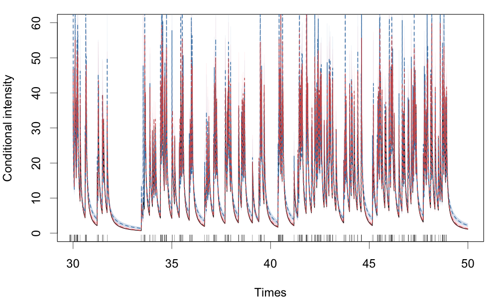
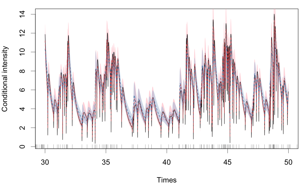
Figure S1: Comparison of Burr MTDPP and Burr ACD models regarding conditional intensity functions evaluated at the time interval $(30,50)$, under the first simulation scenario (left; $(\gamma,\sigma^{2})=(1,0.8))$ and the second simulation scenario (right; $(\gamma,\sigma^{2})=(1.5,0.8))$. The black solid line corresponds to the true conditional intensity of the Burr ACD model. The blue dashed line and blue polygon, respectively, correspond to the posterior mean and the pointwise $95\%$ interval estimates of the conditional intensity for the Burr MTDPP. The red dashed line and red polygon, respectively, correspond to the point and pointwise $95\%$ interval estimates of the conditional intensity for the Burr ACD model.

Burr MTDPP model

We applied the stationary Burr MTDPP model defined in Equation (8) of the main paper, with $L=3$. We assigned $\mathrm{Ga}(1,1)$ priors to $\gamma$ and $\lambda$, respectively, and independently of $(\gamma,\lambda)$, we placed a truncated gamma prior, $\mathrm{Ga}(6,1)\mathbbm{1}(\kappa>1)$, which implies the first five moments of the marginal duration distribution exist. The vector of weights received a CDP$(5,1,2)$ prior. For each scenario, we obtained 5000 posterior samples, collected every tenth iteration from a Markov chain, after discarding the first 5000 samples. We generated posterior predictive samples for in-sample and out-of-sample predictions, respectively, according to (11) and (9).

Table S1:  Comparison of Burr MTDPP and Burr ACD models regarding one-step-ahead in-sample prediction, under each of the two simulation scenarios.

	$\gamma=1,\,\sigma^{2}=0.8$					$\gamma=1.5,\,\sigma^{2}=0.8$
	MAD	RMSE	CRPS	IS		MAD	RMSE	CRPS	IS
ACD	0.07	0.18	0.06	0.96		0.11	0.23	0.09	1.19
MTDPP	0.06	0.18	0.06	0.97		0.10	0.23	0.10	1.15

Table S2:  Comparison of Burr MTDPP and Burr ACD models regarding one-step-ahead out-of-sample prediction, under each of the two simulation scenarios.

	$\gamma=1,\,\sigma^{2}=0.8$					$\gamma=1.5,\,\sigma^{2}=0.8$
	MAD	RMSE	CRPS	IS		MAD	RMSE	CRPS	IS
ACD	0.11	0.14	0.03	0.93		0.16	0.19	0.07	1.06
MTDPP	0.07	0.08	0.03	0.55		0.14	0.16	0.06	0.80

The results of in-sample predictions are shown in Table S1. The in-sample predictive performance of the MTDPP model is almost identical to that of the ACD model, indicating a good model fit. Figure S1 shows the point and interval estimates of the conditional intensity functions for the two models, under the two scenarios. Although the Burr MTDPP’s interval estimates miss some true intensity values, overall, the model is able to produce intensity estimates that resemble the true pattern. Again, note that for this simulation study, the Burr MTDPP is a misspecified model, while we fitted the same Burr ACD used to generate synthetic data.

We next turn to the results on out-of-sample predictive performance. Note that for the ACD model, although we incorporated the condition that the new duration $X_{m+1}>T_{m}-t_{m}$ for out-of-sample predictions (Equation (15)), this condition is not considered in the approach for inference of ACD models (Engle and Russell, 1998), i.e., the point process likelihood normalizing term (the second term in Equation (2) of the main paper) is ignored. Besides, the interval estimates for the ACD model using bootstrap samples (available from the package’s ACD-model-fitting output) can be conservative diciccio1996bootstrap. On the other hand, the MTDPP’s model inference takes into consideration the likelihood normalizing term, and the model bases its predictions on its posterior predictive distribution (main paper Section 3.3, and Supplementary Material Section S3). Thus, although the Burr ACD model was correctly specified, the Burr MTDPP outperformed the Burr ACD model in both scenarios (see Table S2).

Overall, the simulation study demonstrates the MTDPP’s ability to predict future events and quantify uncertainty under misspecification.

S5.2 Second simulation study: Sensitivity analyses

We conducted a sensitivity analysis for $L$, the number of mixture components, and a prior sensitivity analysis for the mixture weights through a simulation study. Specifically, we generated data from the stationary Burr MTDPP models, with component parameters $(\lambda,\gamma,\kappa)=(1,2,6)$ and weights $\bm{w}=(0.3,0.2,0.01,0.29,0.2)$. We chose observation windows $(0,500)$, $(0,2000)$, $(0,5500)$, resulting in $n=1128$, $4675$, $12743$ event times, respectively. Figure S2 shows the partial autocorrelation functions (PACFs) of the simulated data sets.

Sensitivity analysis for the number of mixture components

Since the PACFs of the simulated data sets cut off after lag $5$ or lag $6$, we chose $L=$ $10$, $15$, and $20$ for the sensitivity analysis. For each one of the observation windows, we fitted the Burr MTDPP model with $L=$ $10$, $15$, and $20$, respectively, with priors for the weights, $\mathrm{CDP}(5,1,5)$, $\mathrm{CDP}(5,1,6)$, $\mathrm{CDP}(5,1,8)$. We assigned $\mathrm{Ga}(1,1)$ prior to $\gamma$, and independently of $\gamma$, we placed a truncated gamma prior, $\mathrm{Ga}(6,1)\mathbbm{1}(\kappa>1)$, on $\kappa$. The scale parameter $\lambda$ was assigned a $\mathrm{Ga}(1,1)$ prior.

Figure S3 and Table S3 illustrate the posterior means and $95\%$ credible interval estimates, respectively, for the weights and for the component-density parameters. All the results were based on posterior samples collected every sixteenth iteration from a Markov chain of 85000 iterations with a burn-in of 5000 samples. We observed that the estimates were quite consistent for different values of $L$, and the model was able to penalize non-influential lags by assigning them small probabilities.

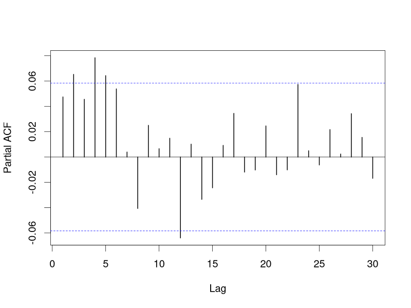
(a) PACF ($n=1128$)

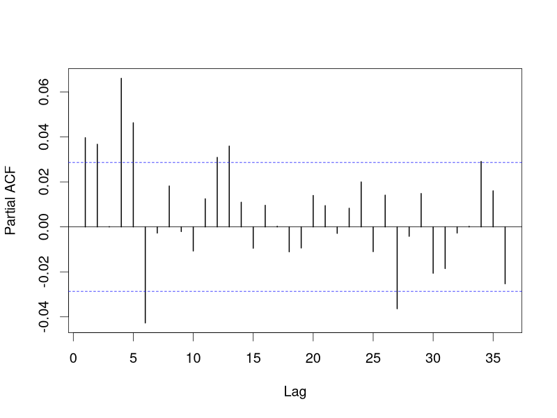
(b) PACF ($n=4675$)

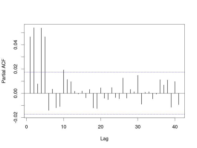
(c) PACF ($n=12473$)

Figure S2: PACFs of the three simulated data sets used in the sensitivity analysis for $L$, the number of mixture components.

Table S3: Posterior mean and $95\%$ credible interval estimates of the parameters $\lambda$, $\gamma$, and $\kappa$, with $L=$ $10$, $15$, and $20$, for observation windows: $(0,500)$ ($n=1128$), $(0,2000)$ ($n=4675$), and $(0,5500)$ ($n=12743$).

	$L=10$	$L=15$	$L=20$
		$n=1128$
$\lambda$	0.96 (0.72, 1.32)	0.95 (0.72, 1.29)	0.96 (0.74, 1.30)
$\gamma$	1.94 (1.81, 2.07)	1.94 (1.82, 2.07)	1.94 (1.82, 2.07)
$\kappa$	5.31 (3.76, 7.69)	5.23 (3.76, 7.57)	5.30 (3.85, 7.62)
		$n=4675$
$\lambda$	1.02 (0.87, 1.19)	1.02 (0.87, 1.20)	1.03 (0.88, 1.22)
$\gamma$	1.97 (1.91, 2.04)	1.97 (1.91, 2.03)	1.97 (1.90, 2.03)
$\kappa$	6.12 (4.96, 7.52)	6.12 (5.03, 7.51)	6.20 (5.07, 7.67)
		$n=12743$
$\lambda$	1.02 (0.93, 1.13)	1.01 (0.92, 1.11)	1.01 (0.92, 1.11)
$\gamma$	1.98 (1.94, 2.02)	1.98 (1.94, 2.02)	1.98 (1.94, 2.02)
$\kappa$	6.06 (5.38, 6.91)	6.03 (5.31, 6.83)	6.00 (5.33, 6.76)

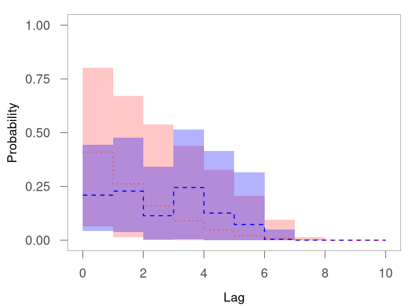
(a) $L=10$, $n=1128$

(b) $L=15$, $n=1128$

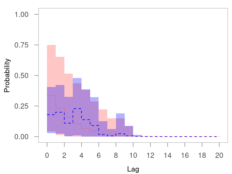
(c) $L=20$, $n=1128$

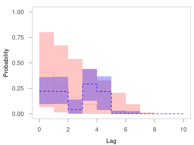
(d) $L=10$, $n=4675$

(e) $L=15$, $n=4675$

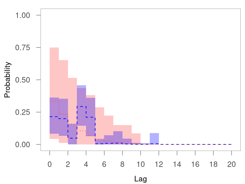
(f) $L=20$, $n=4675$

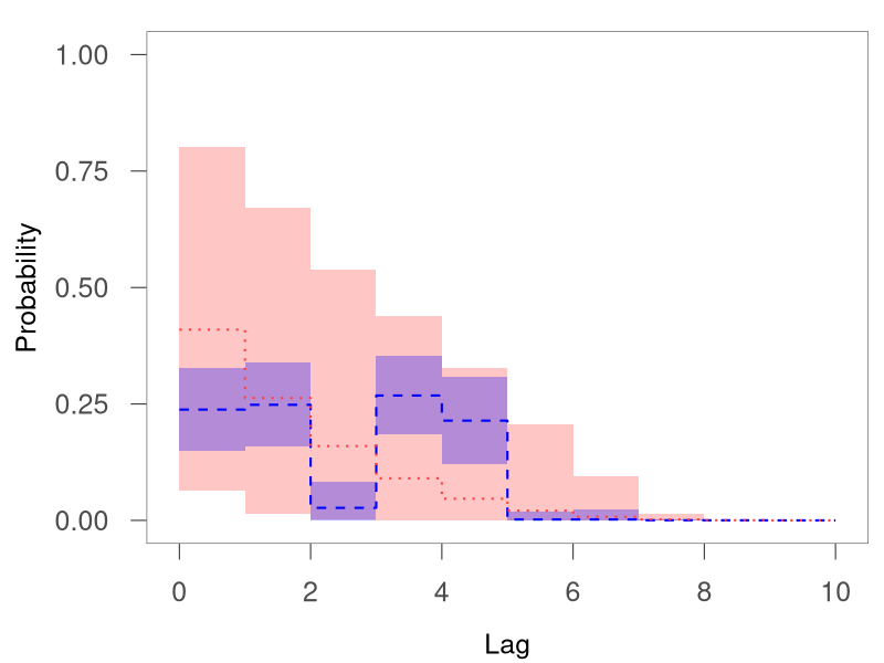
(g) $L=10$, $n=12743$

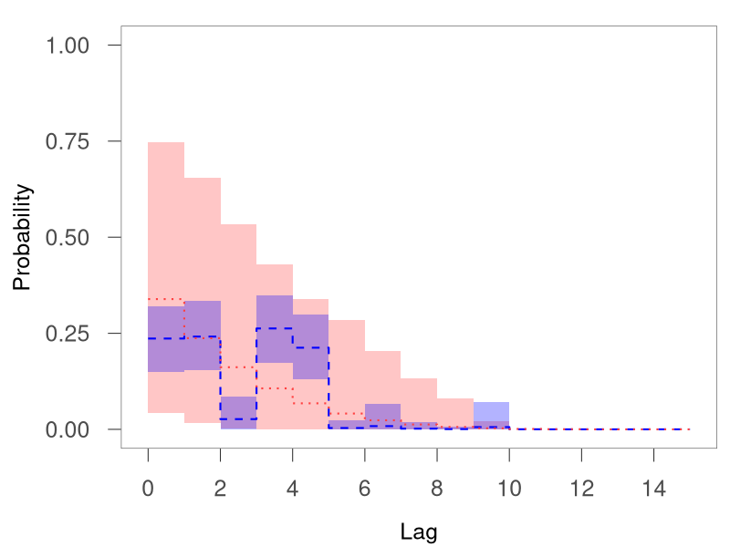
(h) $L=15$, $n=12743$

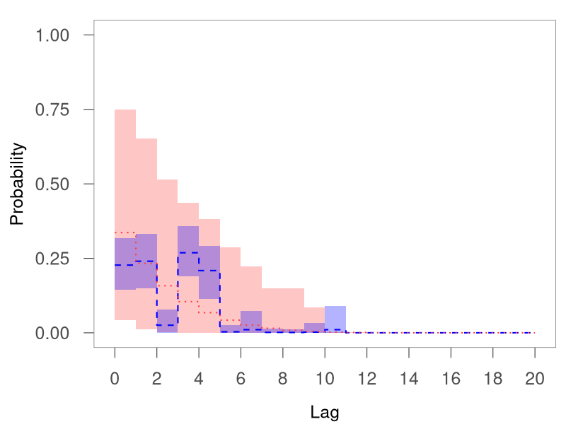
(i) $L=20$, $n=12743$

Figure S3: Posterior mean and $95\%$ credible interval estimates of the mixture weights, under $L=10$ (left column), $L=15$ (middle column), and $L=20$ (right column), for observation windows: $(0,500)$ ($n=1128$; first row), $(0,2000)$ ($n=4675$; second row), and $(0,5500)$ ($n=12743$; third row). Blue lines and blue polygons correspond to posterior mean and interval estimates, while red lines and red polygons correspond to prior mean and interval estimates.

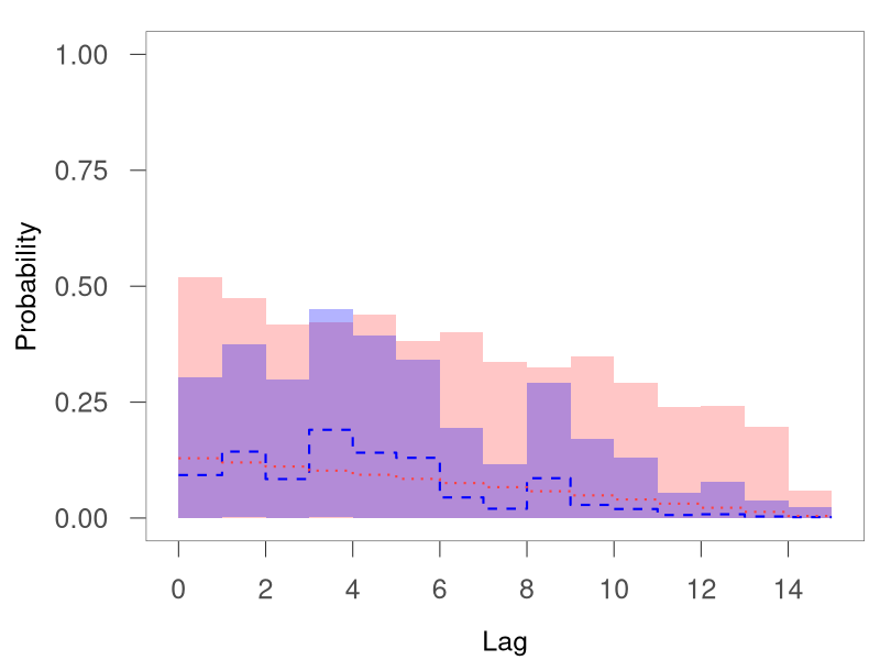
(a) $b_{0}=2$, $n=1128$

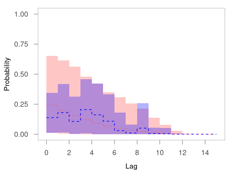
(b) $b_{0}=4$, $n=1128$

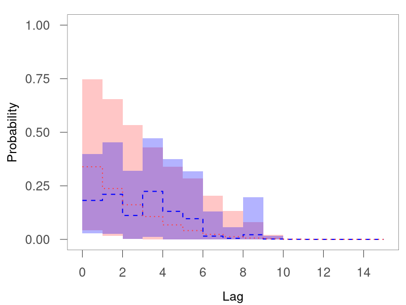
(c) $b_{0}=6$, $n=1128$

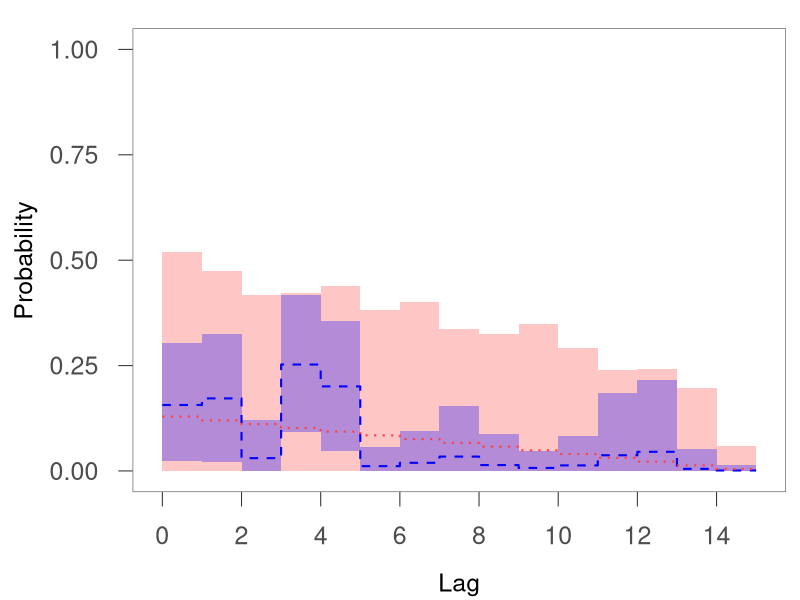
(d) $b_{0}=2$, $n=4675$

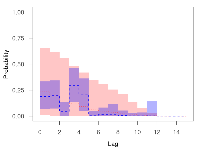
(e) $b_{0}=4$, $n=4675$

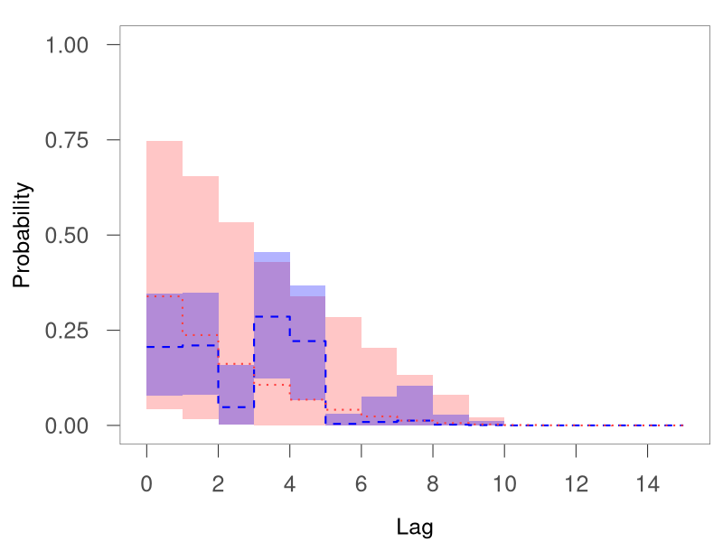
(f) $b_{0}=6$, $n=4675$

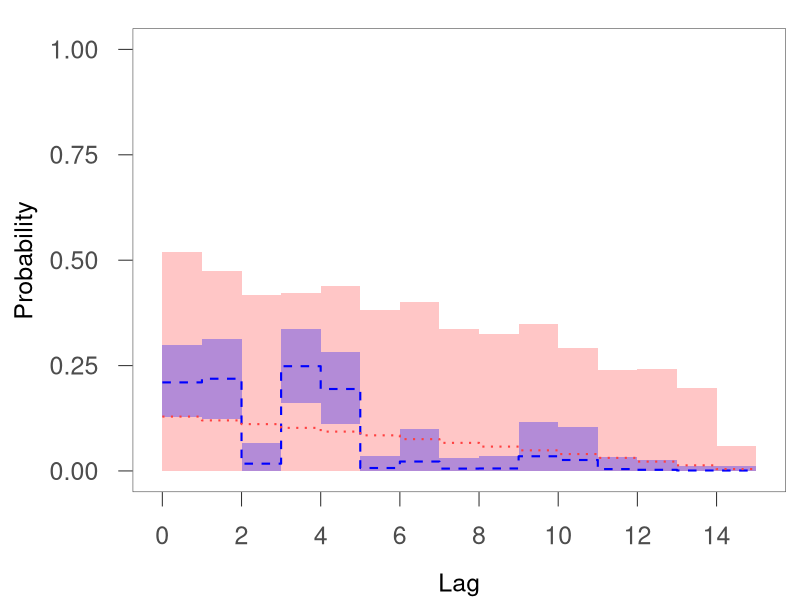
(g) $b_{0}=2$, $n=12743$

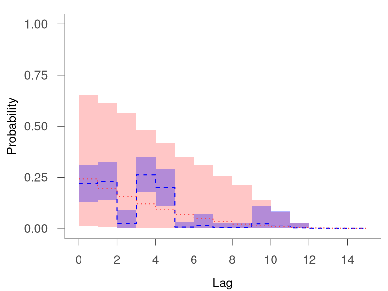
(h) $b_{0}=4$, $n=12743$

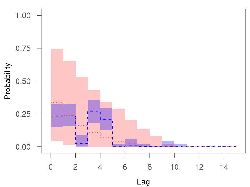
(i) $b_{0}=6$, $n=12743$

Figure S4: Posterior mean and $95\%$ credible interval estimates of the mixture weights, under priors $\mathrm{CDP}(5,1,b_{0})$, with $b_{0}=2$ (left column), $b_{0}=4$ (middle column), and $b_{0}=6$ (right column), for observation windows: $(0,500)$ ($n=1128$; first row), $(0,2000)$ ($n=4675$; second row), and $(0,5500)$ ($n=12743$; third row). Blue lines and blue polygons correspond to posterior mean and interval estimates, while red lines and red polygons correspond to prior mean and interval estimates.

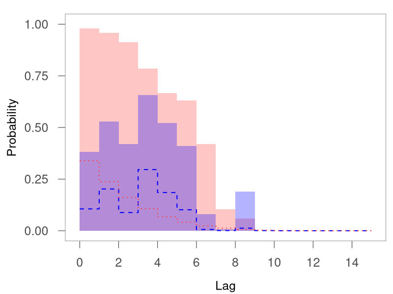
(a) $\alpha_{0}=1$, $n=1128$

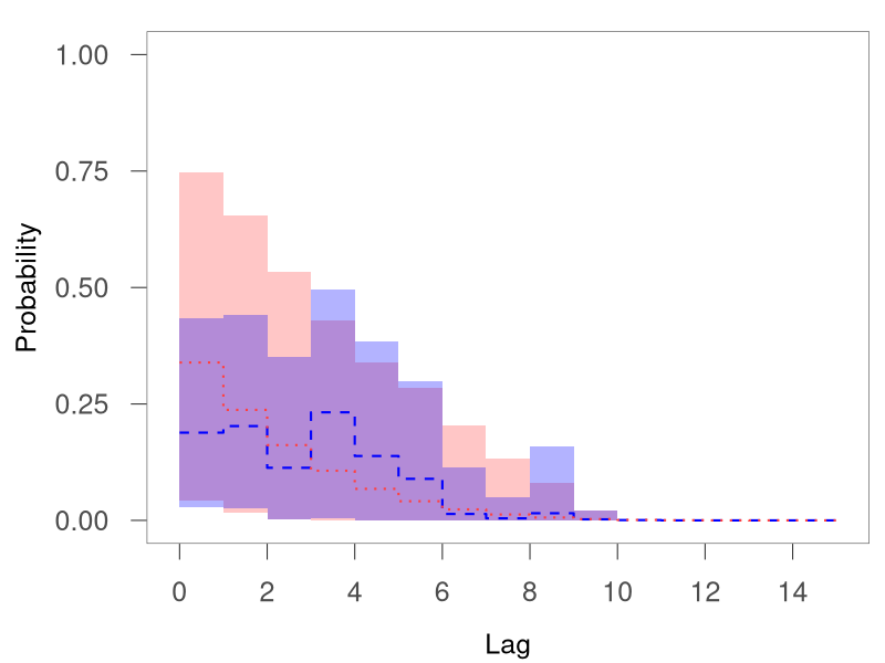
(b) $\alpha_{0}=5$, $n=1128$

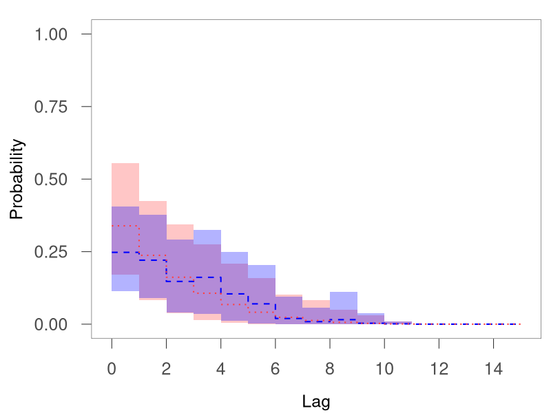
(c) $\alpha_{0}=20$, $n=1128$

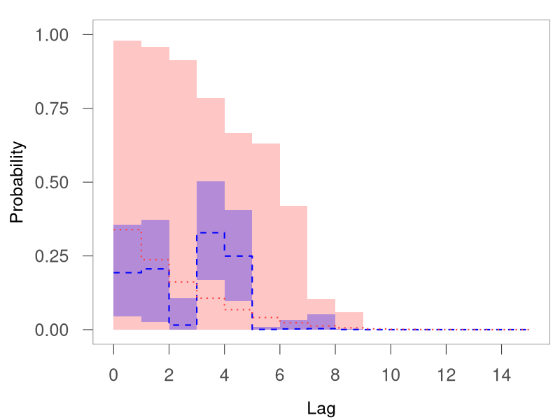
(d) $\alpha_{0}=1$, $n=4675$

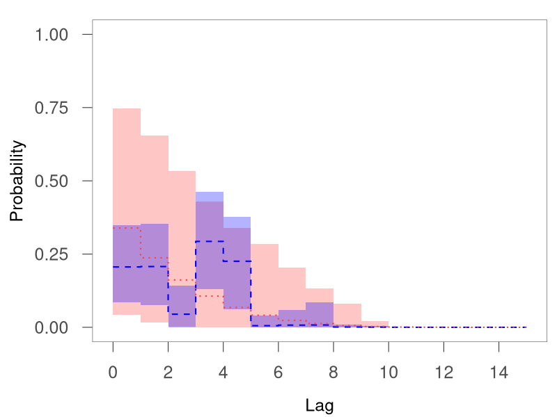
(e) $\alpha_{0}=5$, $n=4675$

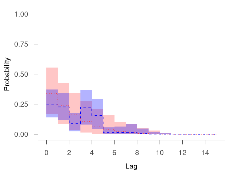
(f) $\alpha_{0}=20$, $n=4675$

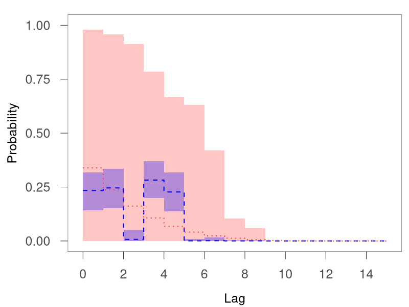
(g) $\alpha_{0}=1$, $n=12743$

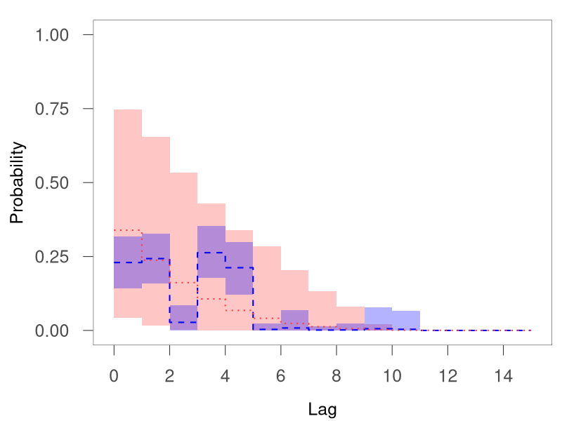
(h) $\alpha_{0}=5$, $n=12743$

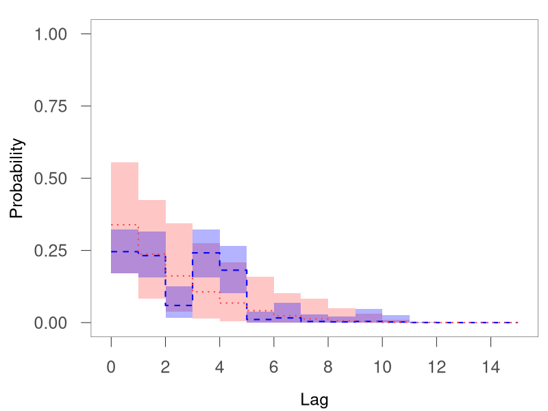
(i) $\alpha_{0}=20$, $n=12743$

Figure S5: Posterior mean and $95\%$ credible interval estimates of the mixture weights, under priors $\mathrm{CDP}(\alpha_{0},1,6)$, with $\alpha_{0}=1$ (left column), $\alpha_{0}=5$ (middle column), and $\alpha_{0}=20$ (right column), for observation windows: $(0,500)$ ($n=1128$; first row), $(0,2000)$ ($n=4675$; second row), and $(0,5500)$ ($n=12743$; third row). Blue lines and blue polygons correspond to posterior mean and interval estimates, while red lines and red polygons correspond to prior mean and interval estimates.

Prior sensitivity analysis for the mixture weights

The sensitivity analysis for $L$ suggested that $L=15$ worked as a reasonable upper bound. Thus, for the following prior sensitivity analysis, we chose $L=15$ when fitting models. For each one of the observation windows, we first fitted the Burr MTDPP model, using priors for the weights, $\mathrm{CDP}(5,1,b_{0})$, with $b_{0}=2,4,6$; then we fitted the Burr model using $\mathrm{CDP}(\alpha_{0},1,6)$ with $\alpha_{0}=1,5,20$. Thus, in total, we fitted the model six times for each observation window. The posterior estimates of the weights are summarized in Figures S4 and S5. All the results were based on posterior samples collected every sixteenth iteration from a Markov chain of 85000 iterations with a burn-in of 5000 samples.

Figure S4 shows the posterior mean and interval estimates of the weights under priors, $\mathrm{CDP}(5,1,2)$, $\mathrm{CDP}(5,1,4)$, and $\mathrm{CDP}(5,1,6)$. As $b_{0}$ increases, the model imposes a greater penalty on distant lags, resulting in less uncertainty. Regardless of the choice of $b_{0}$, the posterior estimates of the weights generally recovered the pattern of the true weights, i.e., there is a gap between the first two and the last two influential lags. Moreover, the posterior estimates become closer to the true weights as $n$ increases.

Table S4:  Posterior mean and $95\%$ credible interval estimates of the component parameter estimates $\lambda$, $\gamma$, and $\kappa$, under priors $\mathrm{CDP}(5,1,b_{0})$, with $b_{0}=2,4,6$.

	$b_{0}=2$	$b_{0}=4$	$b_{0}=6$
		$n=1128$
$\lambda$	0.93 (0.71, 1.21)	0.95 (0.71, 1.31)	0.93 (0.71, 1.20)
$\gamma$	1.96 (1.84, 2.09)	1.95 (1.82, 2.09)	1.95 (1.84, 2.08)
$\kappa$	5.09 (3.71, 7.01)	5.23 (3.70, 7.71)	5.07 (3.71, 6.90)
		$n=4675$
$\lambda$	1.00 (0.83, 1.21)	1.02 (0.86, 1.20)	1.02 (0.87, 1.21)
$\gamma$	1.98 (1.91, 2.05)	1.97 (1.91, 2.03)	1.97 (1.91, 2.03)
$\kappa$	5.95 (4.75, 7.59)	6.10 (4.94, 7.58)	6.15 (5.00, 7.70)
		$n=12743$
$\lambda$	0.99 (0.89, 1.10)	1.00 (0.90, 1.11)	1.01 (0.92, 1.12)
$\gamma$	1.99 (1.95, 2.03)	1.99 (1.94, 2.03)	1.98 (1.94, 2.02)
$\kappa$	5.86 (5.13, 6.70)	5.93 (5.20, 6.79)	5.98 (5.30, 6.83)

Table S5:  Posterior mean and $95\%$ credible interval estimates of the component-density parameters $\lambda$, $\gamma$, and $\kappa$, under priors $\mathrm{CDP}(\alpha_{0},1,6)$, with $\alpha_{0}=1,5,10$.

	$\alpha_{0}=1$	$\alpha_{0}=5$	$\alpha_{0}=20$
		$n=1128$
$\lambda$	1.00 (0.75, 1.38)	0.96 (0.73, 1.29)	0.93 (0.71, 1.24)
$\gamma$	1.93 (1.81, 2.06)	1.94 (1.82, 2.07)	1.95 (1.83, 2.08)
$\kappa$	5.54 (3.91, 8.22)	5.27 (3.82, 7.51)	5.08 (3.70, 7.23)
		$n=4675$
$\lambda$	1.02 (0.86, 1.20)	1.02 (0.88, 1.19)	1.04 (0.88, 1.22)
$\gamma$	1.97 (1.91, 2.04)	1.97 (1.91, 2.03)	1.97 (1.90, 2.03)
$\kappa$	6.14 (4.93, 7.56)	6.13 (5.01, 7.50)	6.25 (5.08, 7.72)
		$n=12743$
$\lambda$	1.02 (0.93, 1.13)	1.01 (0.92, 1.12)	1.00 (0.90, 1.10)
$\gamma$	1.98 (1.94, 2.02)	1.98 (1.94, 2.02)	1.99 (1.95, 2.02)
$\kappa$	6.11 (5.40, 6.91)	6.01 (5.30, 6.84)	5.93 (5.21, 6.72)

Figure S5 shows the posterior mean and interval estimates of the weights under priors, $\mathrm{CDP}(1,1,6)$, $\mathrm{CDP}(5,1,6)$, and $\mathrm{CDP}(20,1,6)$. Note that for the DP that defines the weights, $\alpha_{0}$ is the precision parameter. That is, for large $\alpha_{0}$, there is small variability in the DP realizations, and thus the prior realizations of the weights are less variable as $\alpha_{0}$ increases, as shown in Figure S5. When $\alpha=20$ and the sample size is small (e.g., $n=1128$), the results were sensitive to the prior (Figure S5(c)). However, in other cases, the posterior estimates of the weights were able to recover the true pattern. In all scenarios, the posterior estimates approach the true weights as $n$ increases.

Overall, the prior for the mixture weights, with careful choices of $\alpha_{0}$ and $b_{0}$, is quite robust, in the sense that given the data, the model can assign large weights to influential lags and small probabilities to non-important lags. Tables S4 and S5 show the posterior mean and $95\%$ credible interval estimates of the component-parameter estimates.

S5.3 Third simulation study: The MTDCPP model for event clustering

The goal of this study is to examine the ability of the MTDCPP to recover various clustering behaviors attributed to two different factors. We generate data from a Lomax MTDCPP, that is, with $f_{I}$ corresponding to an exponential distribution with rate parameter $\mu$ and $f^{*}(t-t_{N(t^{-})})$ a stationary Lomax MTDPP.

In the study, we consider four scenarios, with $\pi_{0}$ taking one of the following values, $(0.2$, $0.5$, $0.8$, $1)$. The first three values indicate the proportion of the duration process affected by a factor through $f_{I}$. When $\pi_{0}=1$, the data are equivalently generated by a Poisson process with rate $\mu$. For all scenarios, we take $\mu=0.2$, $\alpha=5$, $\phi=0.1$ and decaying weights $\bm{w}=(0.35,0.25,0.2,0.1,0.1)^{\top}$.

We applied the Lomax MTDCPP model with $L=5$ to the synthetic data. We specified a beta prior $\mathrm{Beta}(\pi_{0}\,|\,1,1)$ for the probability $\pi_{0}$ and a gamma prior $\mathrm{Ga}(\mu\,|\,1,1)$ for the rate parameter $\mu$. For the stationary Lomax MTDPP, the shape and scale parameters received priors $\mathrm{Ga}(\alpha\,|\,6,1)\mathbbm{1}(\alpha>1)$ and $\mathrm{Ga}(\phi\,|\,1,1)$, respectively. In particular, we chose prior for $\alpha$ with the expectation that the first four moments exist with respect to the component and marginal Lomax distributions. The vector $\bm{w}$ was assigned CDP$(\bm{w}\,|\,5,1,3)$, which elicits a decreasing pattern in the weights.

Table S6: Simulation study for event clustering. Posterior mean and $95\%$ credible interval estimates of the MTDCPP model parameters under different scenarios.

	$\pi_{0}=0.2$	$\pi_{0}=0.5$	$\pi_{0}=0.8$	$\pi_{0}=1$
$\pi_{0}$	0.22 (0.20, 0.25)	0.52 (0.48, 0.56)	0.81 (0.76, 0.86)	0.99 (0.96, 1.00)
$\mu$	0.22 (0.19, 0.24)	0.19 (0.17, 0.20)	0.20 (0.19, 0.21)	0.19 (0.18, 0.20)
$\phi$	0.12 (0.09, 0.15)	0.13 (0.09, 0.19)	0.12 (0.02, 0.33)	1.33 (0.04, 4.70)
$\alpha$	5.46 (4.63, 6.43)	6.37 (4.91, 8.15)	4.78 (2.99, 8.21)	5.39 (2.19, 10.82)

We focus on the inference on the two-component mixture probability $\pi_{0}$ and the component density parameters ($\mu,\phi,\alpha$). The posterior mean and $95\%$ credible interval estimates of the parameters are presented in Table S6. The posterior estimates of $\pi_{0}$ suggest that the model was able to recover the proportion of the point process driven by $f_{I}$, even in the extreme case when $\pi_{0}=1$. For other parameters, the model produced estimates close to the true values for all scenarios.

S6 Additional data-example results

S6.1 IVT recurrence interval analysis

Sensitivity analysis of $L$

We first examined the PACF of the durations. As shown in Figure S6(a), the PACF cuts off after lag 1. We then examined the PACF of the detrended durations based on a harmonic regression. That is, we regressed the natural logarithm of duration $x_{i}$ on covariates, $\sin(j\omega t_{i})$ and $\cos(j\omega t_{i})$, $j=1,\dots,J$, where $t_{i}$ is the event time associated with $x_{i}$, $J=5$, $\omega=2\pi/T_{0}$, and $T_{0}=365$. Then, we obtained the detrended durations by taking the exponential of the residuals of the harmonic regression. The PACF of the detrended durations is illustrated in Figure S6(b). Overall, the PACFs indicate the possibility of temporal dependence in the durations.

According to the PACFs, we fitted the multiplicative model (see Section 4.2 of the main paper) with $L=5,10,15,20$, respectively, with priors for the weights, $\mathrm{CDP}(5,1,3)$, $\mathrm{CDP}(5,1,5)$, $\mathrm{CDP}(5,1,6)$, $\mathrm{CDP}(5,1,8)$. For all models, we assigned a normal distribution $N(0,10)$ to each regression parameter. The shape and scale parameters $\alpha$ and $\phi$, respectively, received $\mathrm{Ga}(6,1)\mathbbm{1}(\alpha>1)$ and $\mathrm{Ga}(1,1)$ priors. We examined model performance on parameter estimates, which are demonstrated in Figure S6 and Table S7. Results are based on 5000 posterior samples, obtained after discarding the first 5000 iterations of the MCMC and then retaining one every tenth iterations. Computing times for running the models are also reported in Table S7.

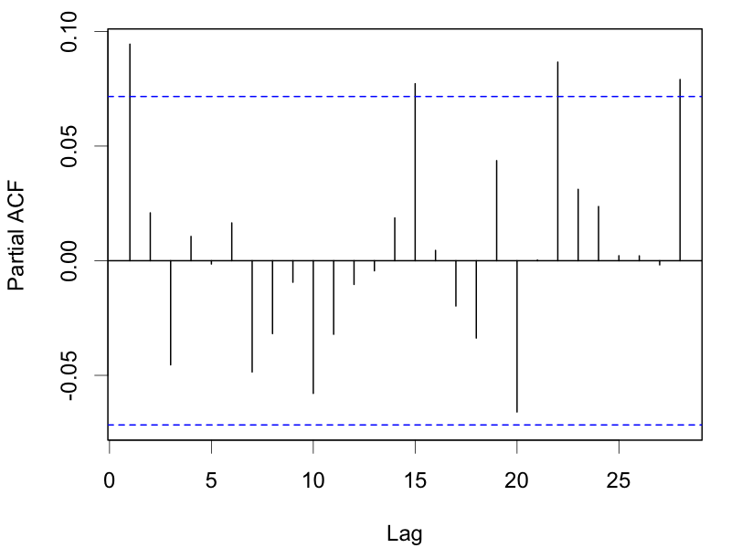
(a) PACF (original data)

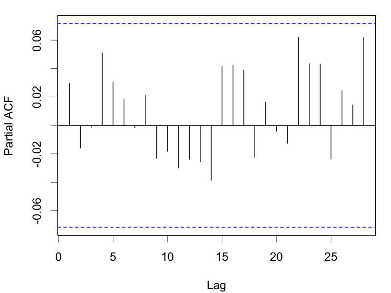
(b) PACF (detrended data)

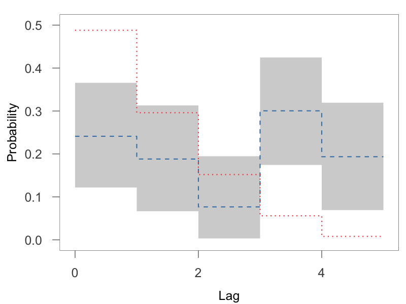
(c) $L=5$

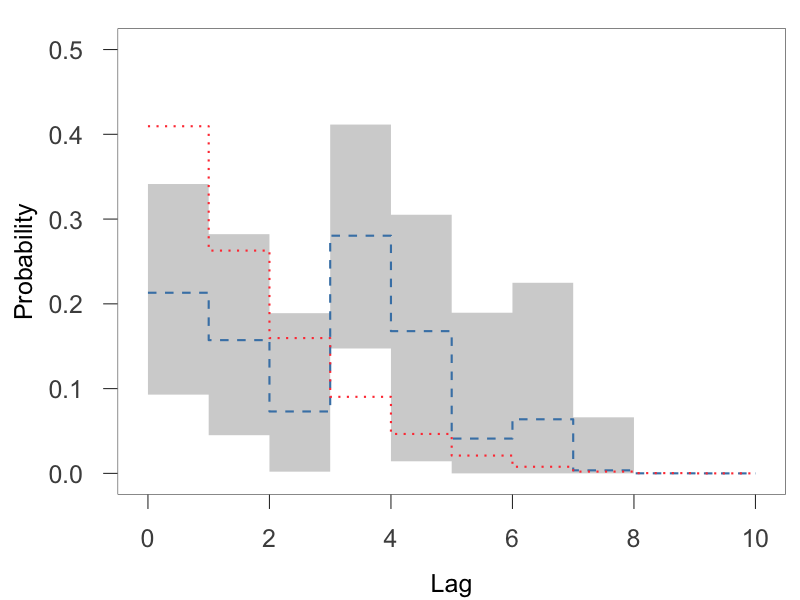
(d) $L=10$

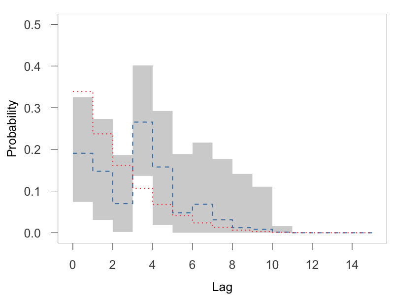
(e) $L=15$

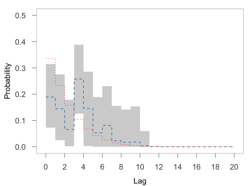
(f) $L=20$

Figure S6: IVT recurrence interval analysis: Partial autocorrelation functions for the original durations (Panel (a)) and for the detrended durations (Panel (b)) based on a harmonic regression; posterior mean and 95% credible interval estimates for the weights, under the MTDPP multiplicative model with $L=5$ (Panel (c)), $L=10$ (Panel (d)), $L=15$ (Panel (e)), and $L=20$ (Panel (f)). Blue dashed lines, red dotted lines, and grey polygons are, respectively, posterior mean, prior mean, are $95\%$ credible interval estimates.

Table S7: IVT recurrence interval analysis (sensitivity analysis of $L$): posterior mean and 95% credible interval estimates for the component-density and harmonic-regression parameters, and computing time (minutes), under the MTDPP multiplicative model with different values of $L$.

	$L=5$	$L=10$	$L=15$	$L=20$
$\alpha$	2.04 (1.75, 2.37)	2.03 (1.75, 2.36)	2.01 (1.73, 2.36)	2.02 (1.73, 2.37)
$\phi$	5.16 (3.55, 7.09)	5.05 (3.46, 7.05)	4.95 (3.38, 6.90)	4.95 (3.35, 6.92)
$\beta_{11}$	-0.58 (-0.85, -0.30)	-0.57 (-0.85, -0.30)	-0.59 (-0.86, -0.30)	-0.59 (-0.87, -0.31)
$\beta_{12}$	-0.67 (-1.03, -0.33)	-0.68 (-1.07, -0.34)	-0.69 (-1.06, -0.35)	-0.70 (-1.07, -0.35)
$\beta_{21}$	0.21 (-0.11, 0.55)	0.20 (-0.12, 0.56)	0.20 (-0.13, 0.52)	0.19 (-0.14, 0.53)
$\beta_{22}$	-0.53 (-0.82, -0.25)	-0.53 (-0.82, -0.24)	-0.53 (-0.82, -0.22)	-0.53 (-0.83, -0.23)
$\beta_{31}$	0.16 (-0.19, 0.49)	0.16 (-0.23, 0.51)	0.16 (-0.19, 0.49)	0.15 (-0.21, 0.50)
$\beta_{32}$	0.04 (-0.20, 0.29)	0.04 (-0.21, 0.29)	0.04 (-0.22, 0.29)	0.04 (-0.21, 0.29)
$\beta_{41}$	-0.06 (-0.34, 0.21)	-0.07 (-0.34, 0.22)	-0.08 (-0.35, 0.20)	-0.08 (-0.37, 0.21)
$\beta_{42}$	0.23 (-0.04, 0.50)	0.24 (-0.03, 0.50)	0.24 (-0.03, 0.52)	0.23 (-0.04, 0.51)
$\beta_{51}$	0.09 (-0.11, 0.29)	0.09 (-0.12, 0.30)	0.09 (-0.12, 0.30)	0.10 (-0.11, 0.31)
$\beta_{52}$	-0.12 (-0.34, 0.09)	-0.13 (-0.34, 0.10)	-0.13 (-0.34, 0.10)	-0.13 (-0.35, 0.09)
Time	17.22	18.95	20.36	21.87

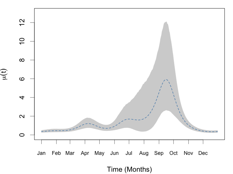
(a) $L=5$

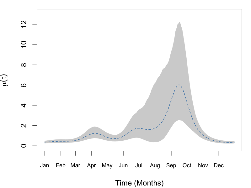
(b) $L=10$

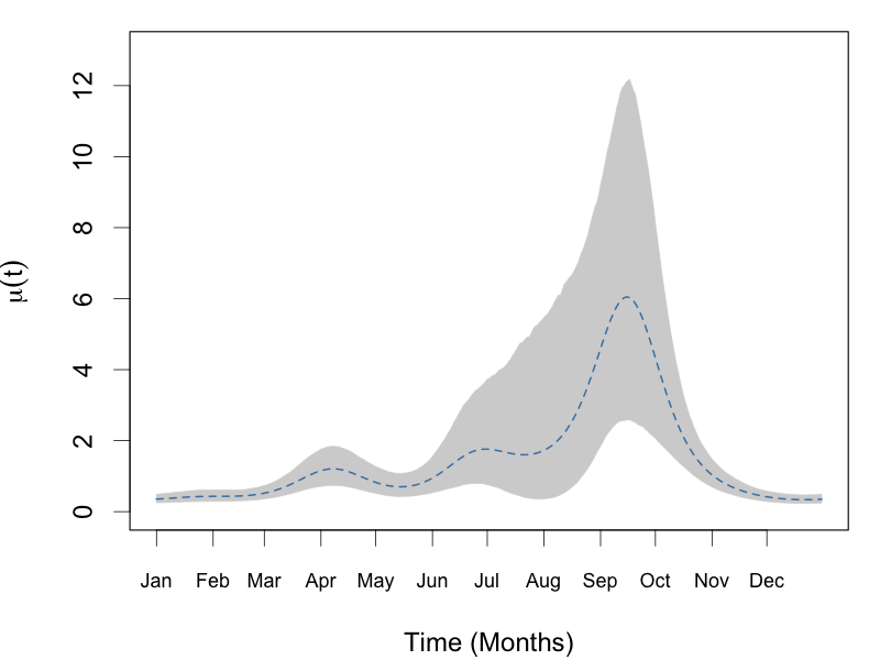
(c) $L=15$

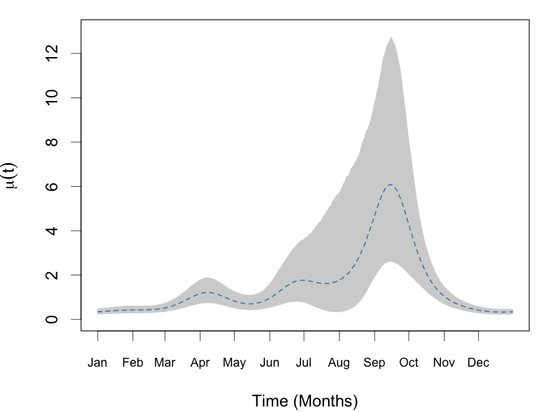
(d) $L=20$

Figure S7: IVT recurrence interval analysis (sensitivity analysis of $L$): harmonic function $\mu(t)$ (for an one-year window) of the MTDPP multiplicative model with different values of $L$.

Figure S6(c)-(f) shows the posterior mean and $95\%$ credible interval estimates of the weights, under different values of $L$. We observed that, $L=5$ seems not large enough to work as an upper bound, but when $L$ ranged from $10$ to $20$, the posterior estimates of the weights were quite consistent. Available in Table S7 are the posterior mean and $95\%$ credible interval estimates of the parameters $\{\alpha,\phi,\bm{\beta}\}$, where $\bm{\beta}=(\beta_{11},\beta_{12},\beta_{21},\beta_{22},\dots,\beta_{51},\beta_{52})^{\top}$. Overall, the estimates of $\{\alpha,\phi,\bm{\beta}\}$ were quite robust across different values of $L$. All the four models implied the presence of annual and semiannual seasonality, and the posterior mean and pointwise $95\%$ credible interval estimates of the harmonic function $\mu(t)$ look similar across different $L$, as shown in Figure S7. Overall, there were no discernible differences among the models with $L$ between $10$ and $20$. Thus, we used $L=15$ as the upper bound for the rest of the analyses for this particular data example.

Comparison with the renewal process

We also assessed model performance by comparison with a renewal process (RP) model, which involves the simpler assumption of independent durations.

The scaled-Lomax RP model is obtained by modeling the $z_{i}$ of the multiplicative model in Section 4.2 of the main paper with an RP, such that the $z_{i}$, $i=1,\dots,n$, are independent and identically distributed as a scaled-Lomax distribution, $P(z\,|\,\alpha\phi,\alpha-1)$. Thus, the scaled-Lomax RP model corresponds to a simpler assumption of the scaled-Lomax MTDPP model in which the $z_{i}$ are identically distributed as $P(z\,|\,\alpha\phi,\alpha-1)$, but are Markov dependent. Our goal is to examine whether incorporating temporal dependence in durations aligns better with the underlying data structure and improves the prediction of future events.

We used the same prior specification for both the scaled-Lomax MTDPP and scaled-Lomax RP models. Specifically, the regression parameter vector was assigned mean-zero dispersed normal priors, and the shape and scale parameters $\alpha$ and $\phi$ received $\mathrm{Ga}(6,1)\mathbbm{1}(\alpha>1)$ and $\mathrm{Ga}(1,1)$ priors, respectively. Both models were fitted with MCMC, and we obtained $5000$ posterior samples with appropriate burn-in and thinning.

To compare the goodness-of-fit of the two models, we used the Bayesian information criterion (BIC; schwarz1978estimating), deviance information criterion (DIC; spiegelhalter2002bayesian), and negative log-likelihood (NLL). Regarding predictive performance, we used the same criteria (i.e., MAD, RMSE, CRPS, IS) and same settings (i.e., one-step-ahead in-sample and one-step-ahead out-of-sample predictions) with Section S5.1.

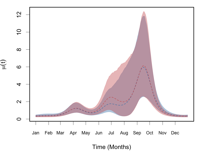
(a) Harmonic functions

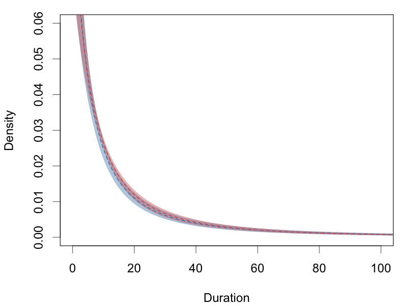
(b) Stationary marginal estimates

Figure S8: IVT recurrence interval analysis: comparison of scaled-Lomax MTDPP (blue) and scaled-Lomax RP (red) models regarding posterior estimates of the harmonic functions and the stationary marginal densities. Dashed lines and polygons correspond to posterior mean and pointwise $95\%$ credible interval estimates, respectively.

Table S8: IVT recurrence interval analysis: comparison of scaled-Lomax MTDPP and scaled-Lomax RP models regarding parameter estimates and goodness-of-fit.

	$\alpha$	$\phi$	DIC	BIC	NLL
MTDPP	2.01 (1.72, 2.35)	4.92 (3.35, 6.92)	5981	6221	3022
RP	2.26 (2.06, 2.51)	6.07 (4.50, 7.98)	6284	6339	3130

Table S9: IVT recurrence interval analysis: comparison of scaled-Lomax MTDPP and scaled-Lomax RP models regarding one-step-ahead in-sample and one-step-ahead out-of-sample predictions.

	In-sample prediction					Out-of-sample prediction
	MAD	RMSE	CRPS	IS		MAD	RMSE	CRPS	IS
MTDPP	14.40	39.91	13.33	202.30		22.08	59.45	11.87	254.96
RP	17.87	179.71	13.28	217.41		30.16	123.52	13.46	414.43

The results in Table S8 suggest that the RP model does not fit the data as well as the MTDPP model, which has smaller values of DIC, BIC, and NLL. Also available in Table S8 are posterior estimates of the parameters for the stationary marginal distribution. The MTDPP model suggests a heavier tail, after adjusting for seasonality. Figure S8 shows the tails of the marginal densities estimated by the two models, as well as the posterior estimates of the harmonic function, where the two models agree on most parts. Turning to predictive performance (Table S9), the MTDPP model not only results in more accurate point predictions, as indicated by much lower RMSEs, but also provides more accurate and tighter prediction intervals, especially when it comes to out-of-sample predictions.

Overall, the comparison demonstrates the benefit of incorporating duration dependence. The scaled-Lomax MTDPP yields better goodness-of-fit, and it improves the prediction of future events for the particular data example.

S6.2 Mid-price changes of the AUD/USD exchange rate

There are $121$ point patterns, each of which corresponds to an one-hour time window during the trading week between July 19 and July 24 in 2015. Before fitting models, we examined the PACF of the durations for each of the $121$ point patterns. Overall, the PACFs first cut off after one of the first five lags. Figure S9(a)-(c) shows the PACFs of three point patterns.

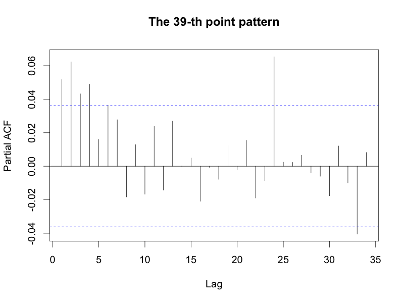
(a) PACF

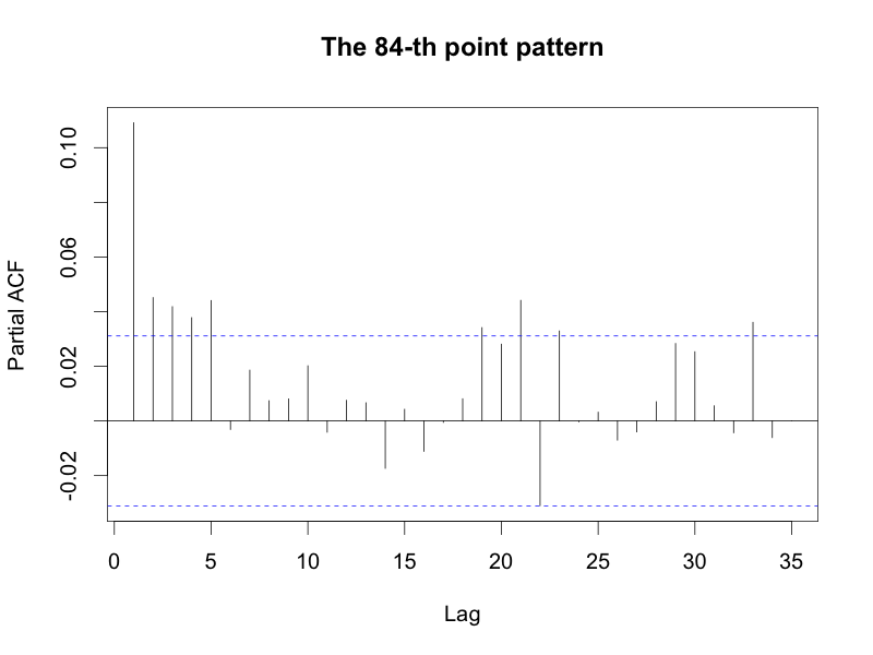
(b) PACF

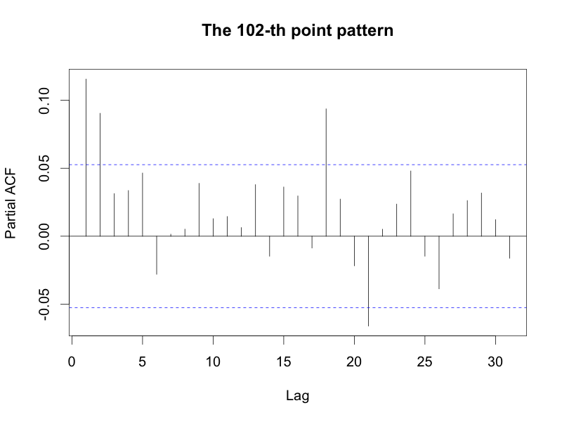
(c) PACF

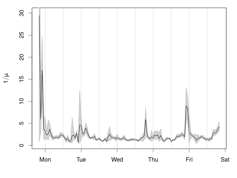
(d) Exponential distribution waiting time $1/\mu$

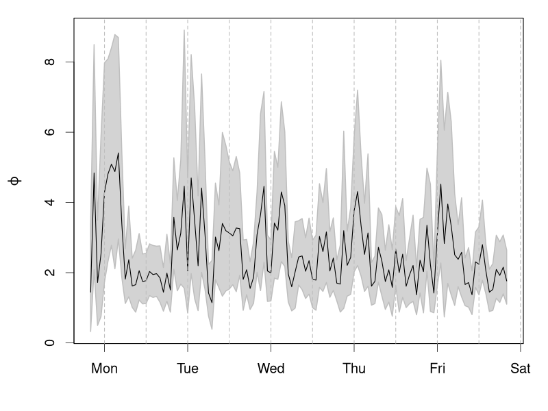
(e) Lomax MTDPP scale parameter $\phi$

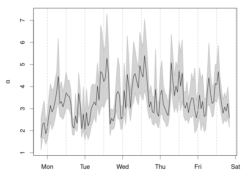
(f) Lomax MTDPP shape parameter $\alpha$

Figure S9: AUD/USD foreign exchange market endogeneity analysis. The top row shows the PACFs for three point patterns. The bottom row plots the time series of the posterior mean (solid lines) and pointwise $95\%$ credible interval (grey polygons) estimates for parameters $1/\mu$, $\phi$, and $\alpha$, based on the MTDCPP model. Vertical dashed lines correspond to midnight and midday GMT.

Figure S9(d)-(f) illustrates the time series of posterior mean and interval estimates for three parameters: exponential distribution parameter $1/\mu$, Lomax MTDPP scale and shape parameters $\phi$ and $\alpha$. Note that the exponential distribution and Lomax MTDPP are regarded as drivers of external and internal factors for waiting times between successive mid-price changes, respectively. The estimates of the mean waiting time $1/\mu$ for external factors shows obvious diurnal pattern, with peaks and troughs appearing around midnight and midday GMT, respectively. The posterior estimates of $\phi$ for all point patterns seem more volatile, with relatively high and low values occurring at midnight and midday GMT, whereas the posterior estimates of $\alpha$ reflect an opposite pattern. The mean of the stationary marginal distribution of the Lomax MTDPP is $\phi/(\alpha-2)$, provided that $\alpha>2$. Thus, given the patterns of estimated $\phi$ and $\alpha$, the estimates of the mean waiting time for internal factors appear high and low around midnight and midday GMT, respectively. In addition, small values of $\alpha$ around midnight GMT suggest a heavy-tailed duration distribution of the Lomax MTDPP during that period. This indicates that mid-price changes tend to cluster around midnight GMT, which corresponds to the opening time of Asian markets (23:00-1:00 GMT).

S7 MCMC diagnostics

We assessed MCMC convergence through trace plots and ACF plots. Diagnostic results for real data examples (Sections 4.2 and 4.3) are, respectively, shown in Figures S10 and S11. Since there were $121$ point patterns used to fit models in Section 4.3, we show diagnostic results for three point patterns in Figure S11 as illustrations. Diagnostic results for simulation studies (Sections 4.1 and S5.3) are available in Figures S12 and S13, respectively.

S8 Point process model checking results

Given observed points $0<t_{1}<\dots<t_{n}<T$, consider random variables $U^{*}_{i}=$ $1-\exp\{-(\Lambda^{*}(t_{i})-\Lambda^{*}(t_{i-1}))\}=F^{*}(t_{i}-t_{i-1})$, $i=L+1,\dots,n$, as described in Section 3.3 of the main paper. If the point process model is correctly specified, the estimates of $(U^{*}_{L+1},\dots,U^{*}_{n})$ will be independently and identically distributed as a standard uniform distribution. Figure S14 consists of quantile-quantile plots of the estimates of $(U^{*}_{L+1},\dots,U^{*}_{n})$ for the simulation study and the first real data example in the main paper, as well as for the additional study in Section S5.3. Figures S15-S18 contain quantile-quantile plots of the estimates of $(U^{*}_{L+1},\dots,U^{*}_{n})$ for the second real data example in the main paper. The graphical model assessment results indicate good model fit for all data examples.

jasa3 ref

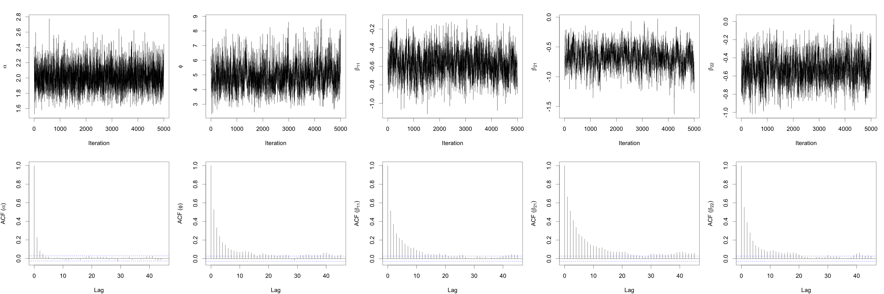
(a)

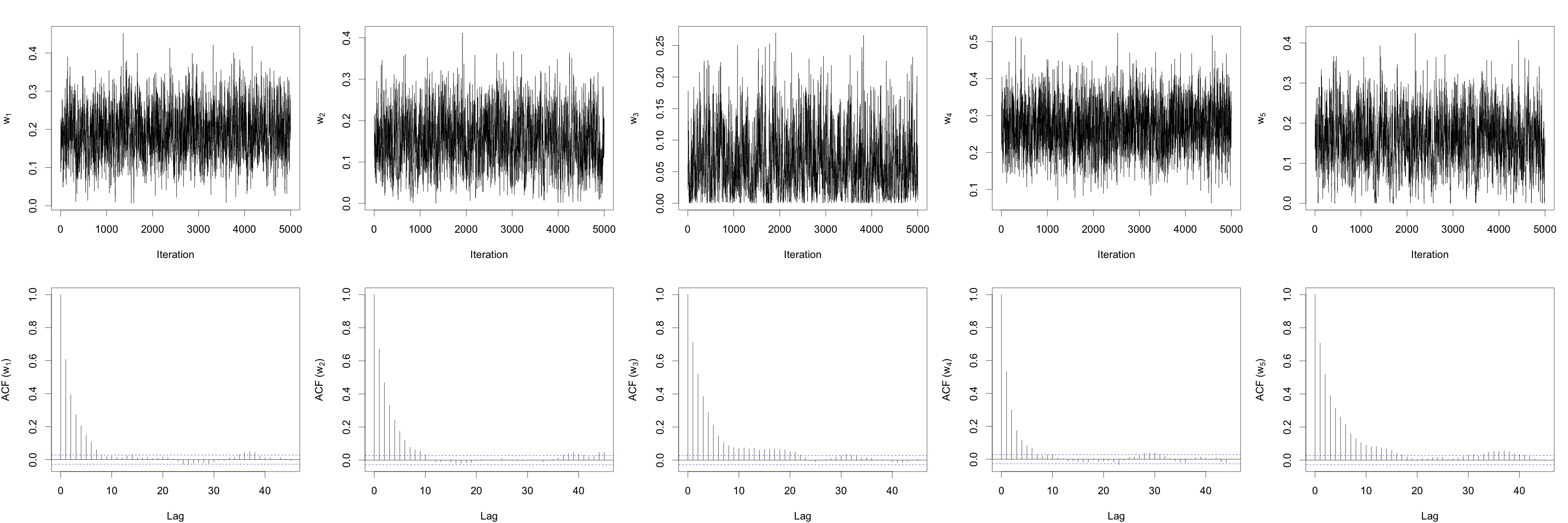
(b)

Figure S10: MCMC convergence diagnostics for Section 4.2 of the main paper: trace plots and ACFs of the posterior samples of the parameters of the scaled-Lomax MTDPP. In Panel (a), columns from left to right correspond to $\alpha$, $\phi$, $\beta_{11}$, $\beta_{21}$, $\beta_{22}$, the last three of which are statistically significant coefficients. In Panel (b), columns from left to right correspond to weights $w_{1}$, $w_{2}$, $w_{3}$, $w_{4}$, and $w_{5}$.

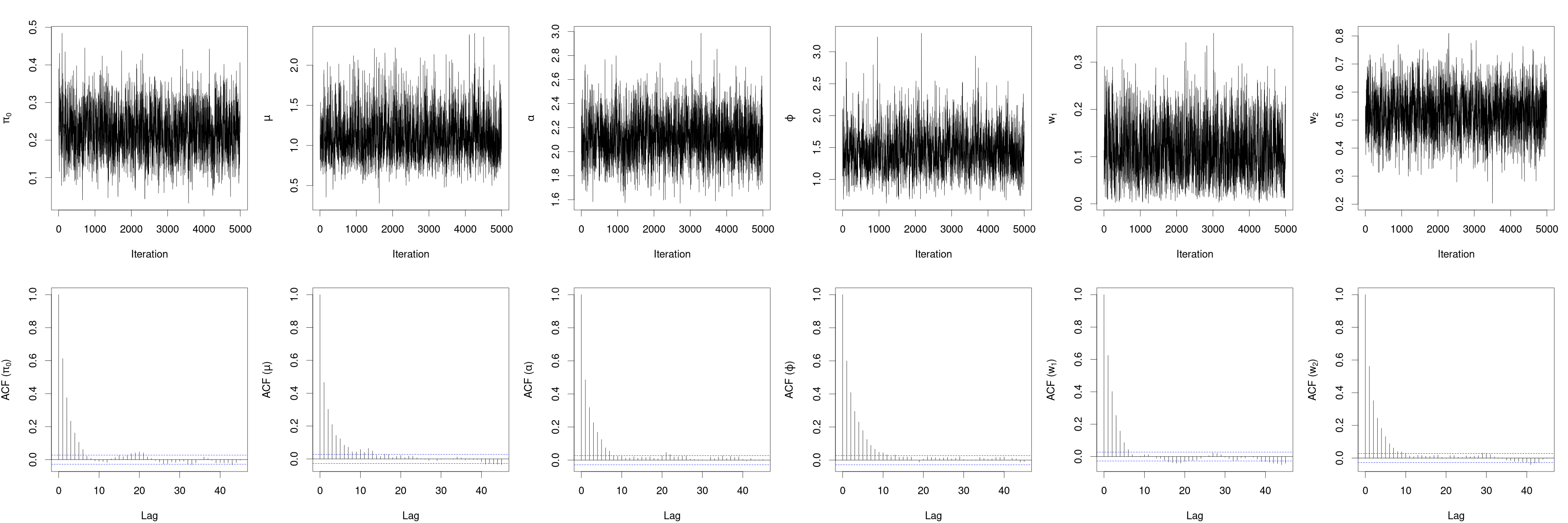
(a)

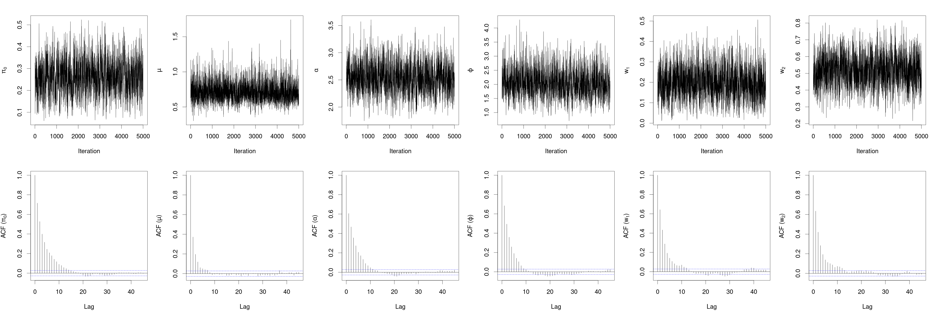
(b)

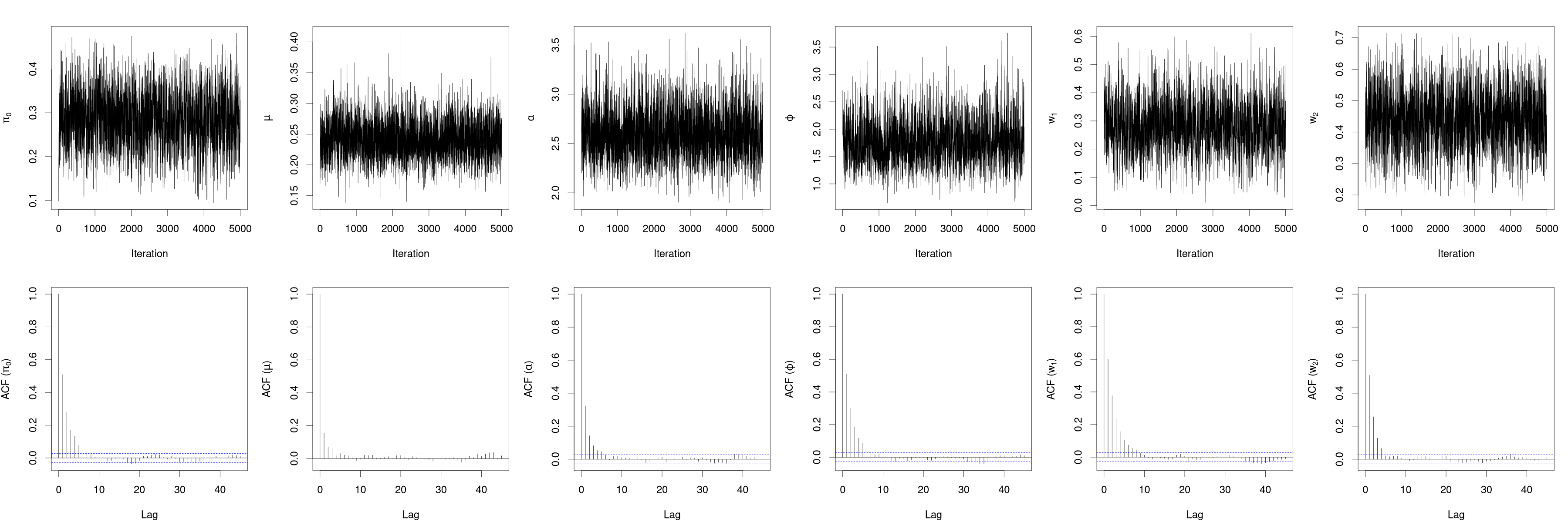
(c)

Figure S11: MCMC convergence diagnostics for Section 4.3 of the main paper: trace plots and ACFs of the posterior samples of the parameters of the Lomax MTDCPP fitted to three point patterns, each of which corresponds to a panel. In each panel, columns from left to right correspond to $\pi_{0}$, $\mu$, $\alpha$, $\phi$, $w_{1}$, and $w_{2}$.

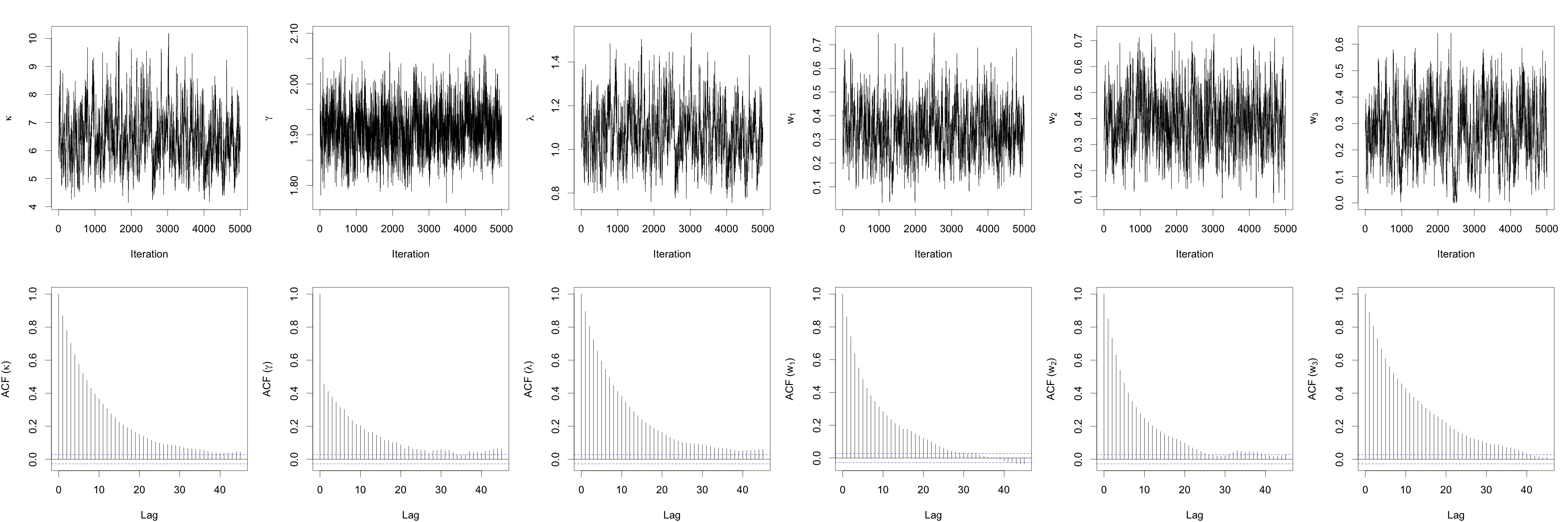
(a)

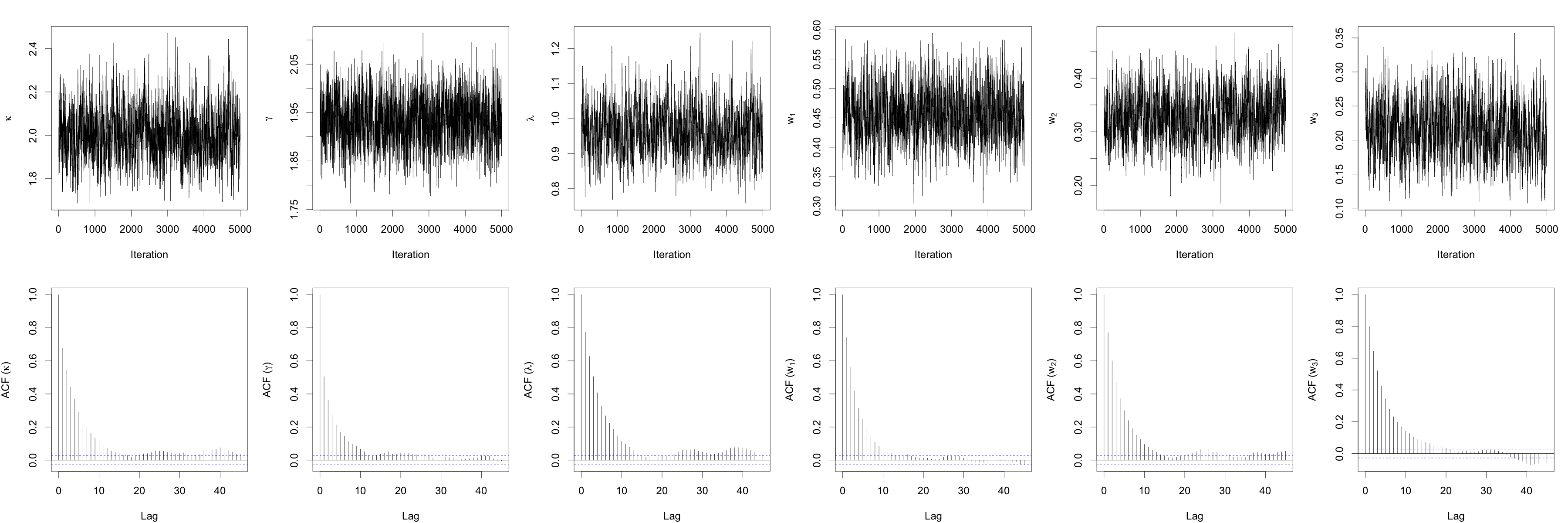
(b)

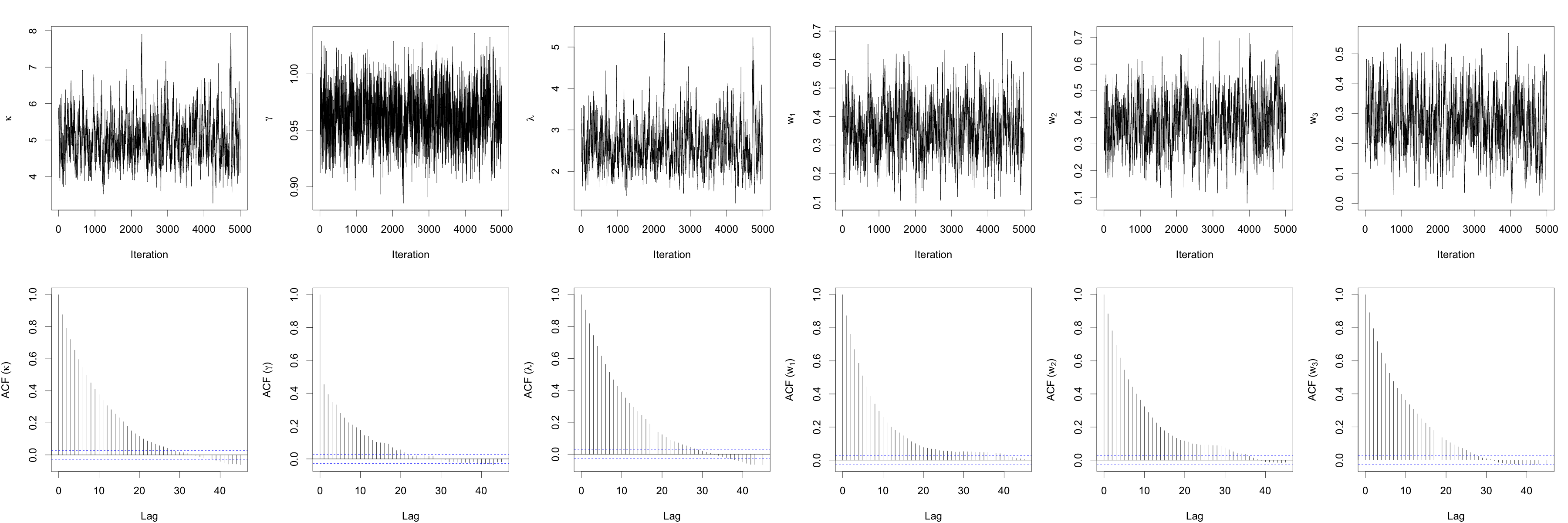
(c)

Figure S12: MCMC convergence diagnostics for Section 4.1 of the main paper: trace plots and ACFs of the posterior samples of the parameters of the Burr MTDPP fitted to data simulated by a a Burr MTDPP(a), a log-logistic MTDPP (b), and a scaled-Lomax MTDPP (c). Columns 1-3 correspond to parameters $\kappa$, $\gamma$, and $\lambda$, and Columns 4-6 correspond to weights $w_{1}$, $w_{2}$, and $w_{3}$.

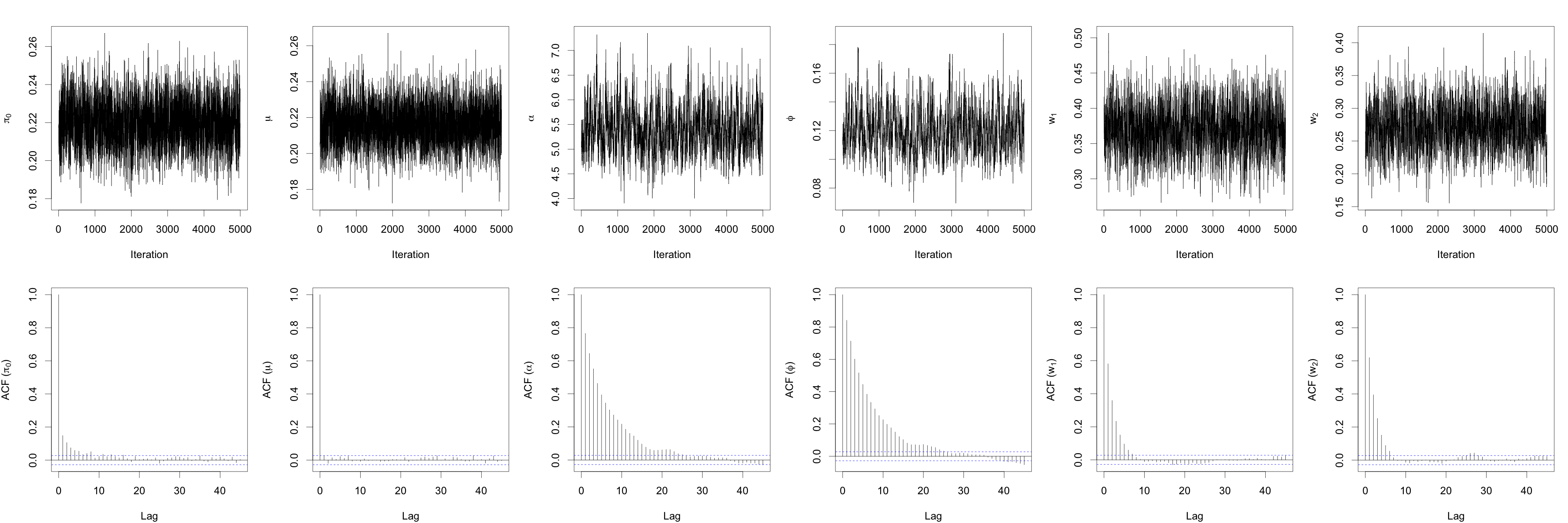
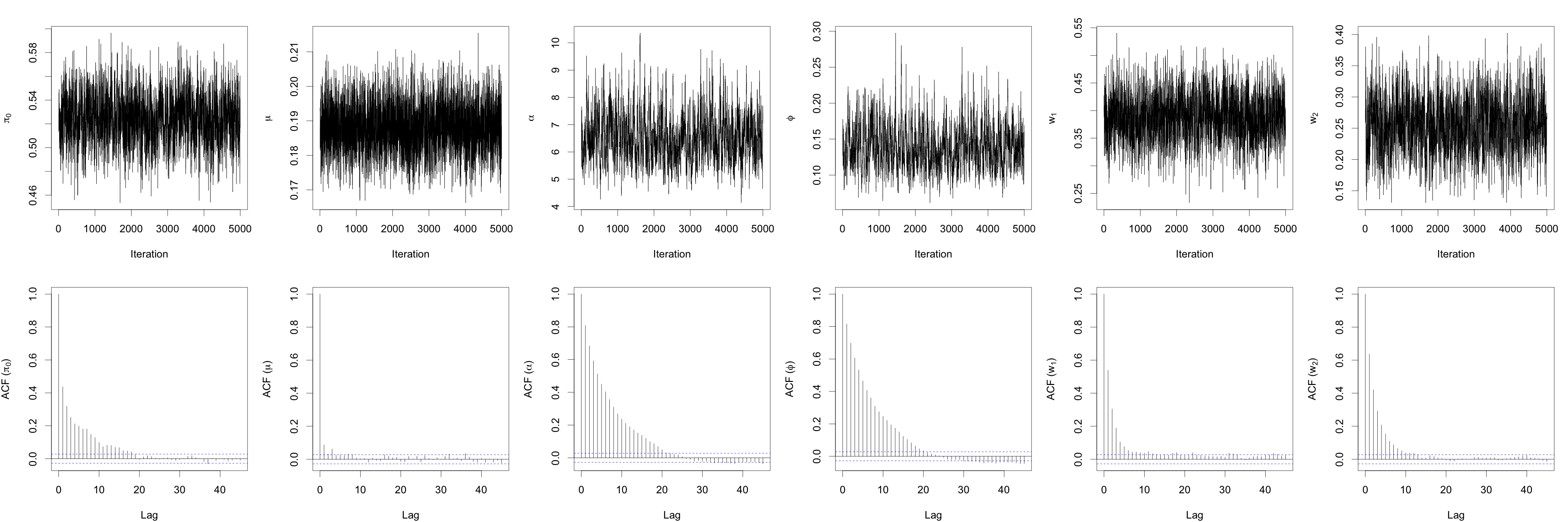
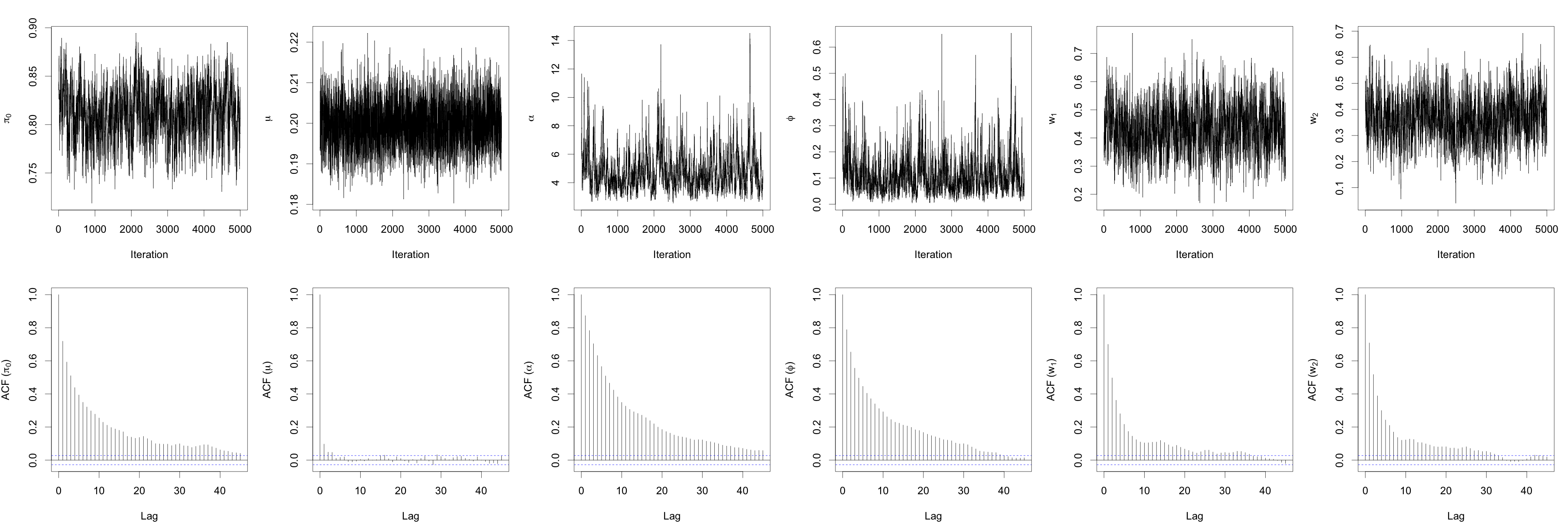
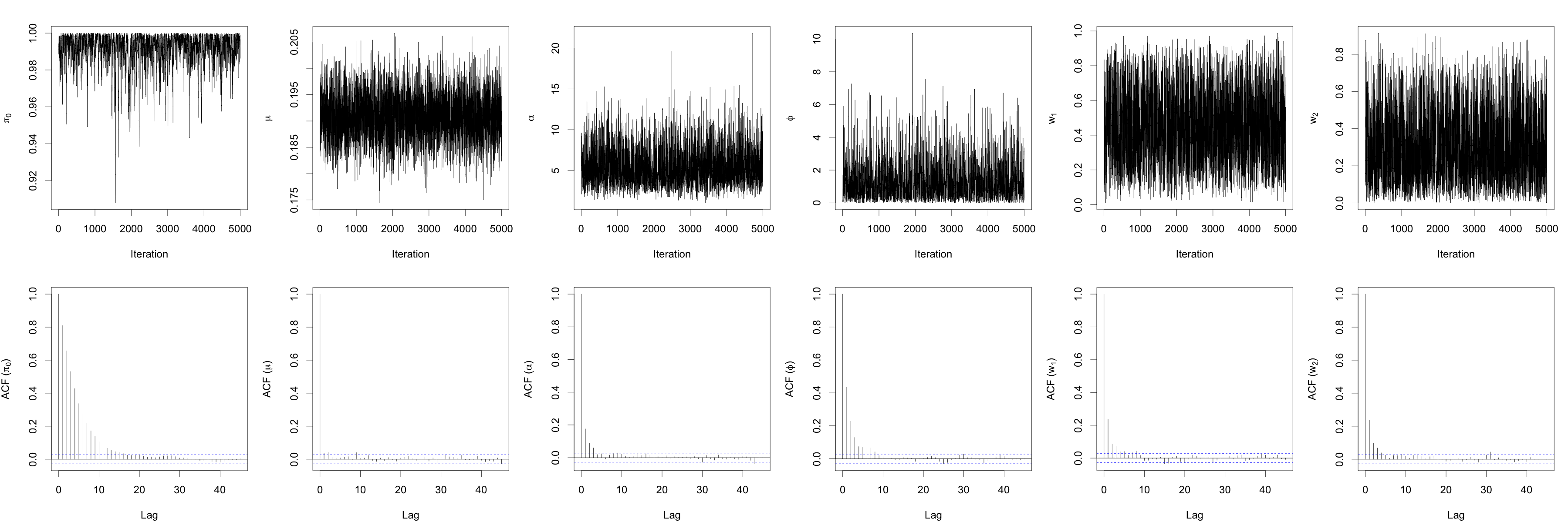
Figure S13: MCMC convergence diagnostics for Section S5.3: From top to bottom are trace plots and ACFs of the posterior samples of the parameters of the Lomax MTDCPP, corresponding to scenarios where $\pi_{0}=0.2$, $0.5$, $0.8$, and $1$.

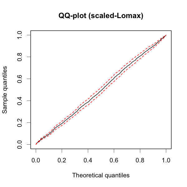
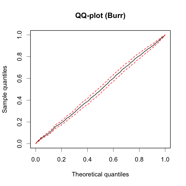
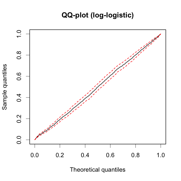
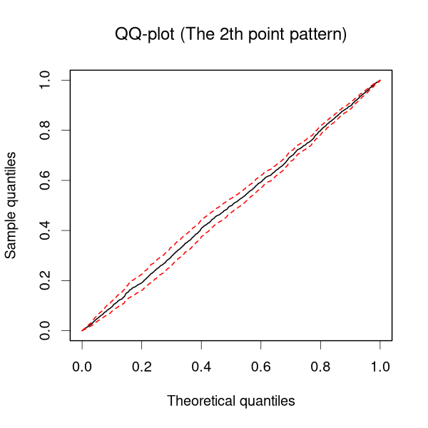
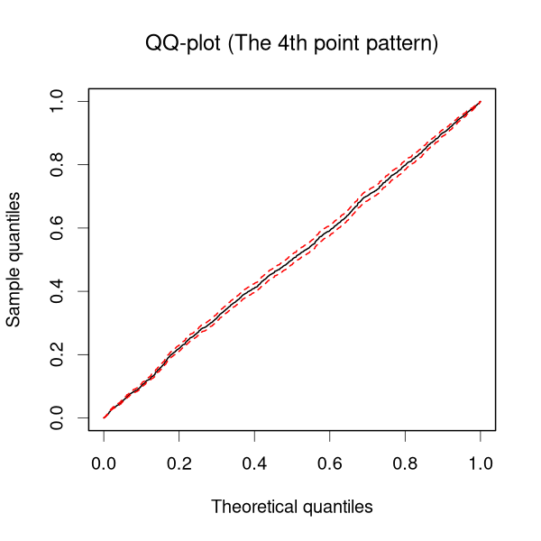
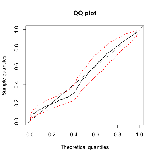
Figure S14: Model checking results. The first row corresponds to the simulation study in the main paper (Section 4.1). The second row and the first panel of the third row correspond to the additional simulation study (Section S5.3). The second panel of the third row corresponds to the IVT data example in the main paper (Section 4.2). Black solid lines and red dotted lines are posterior mean 95% credible interval estimates, respectively.

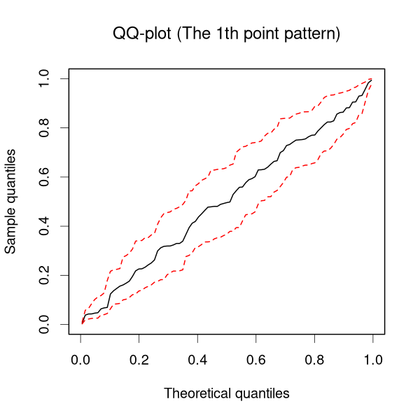
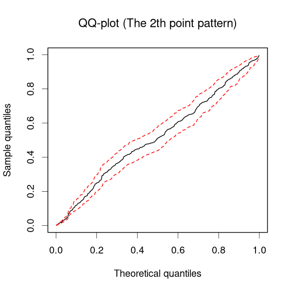
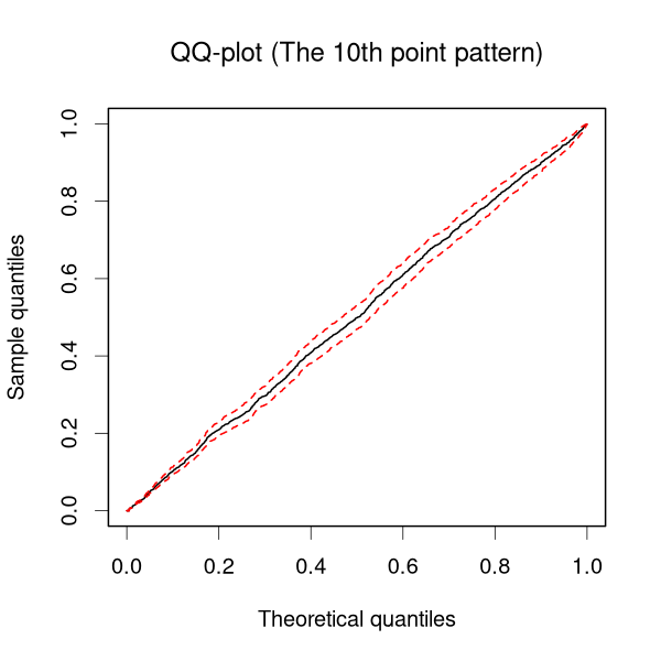
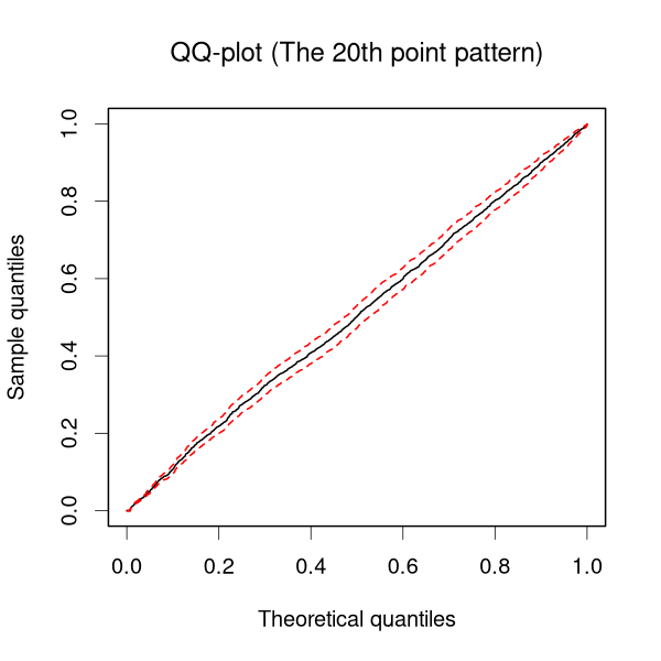
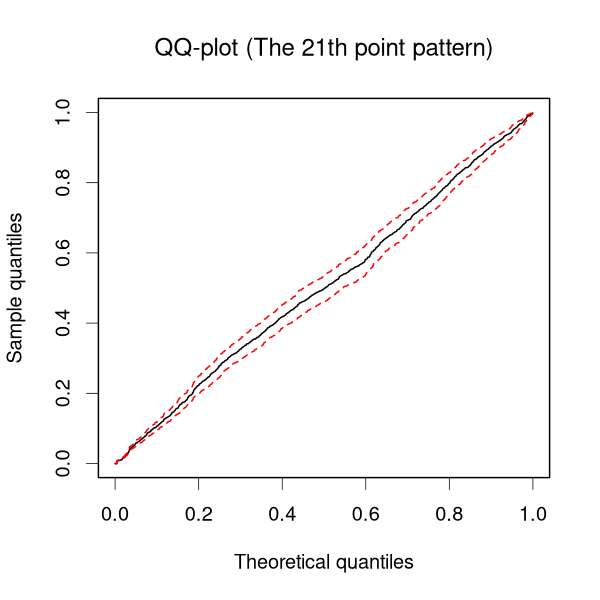
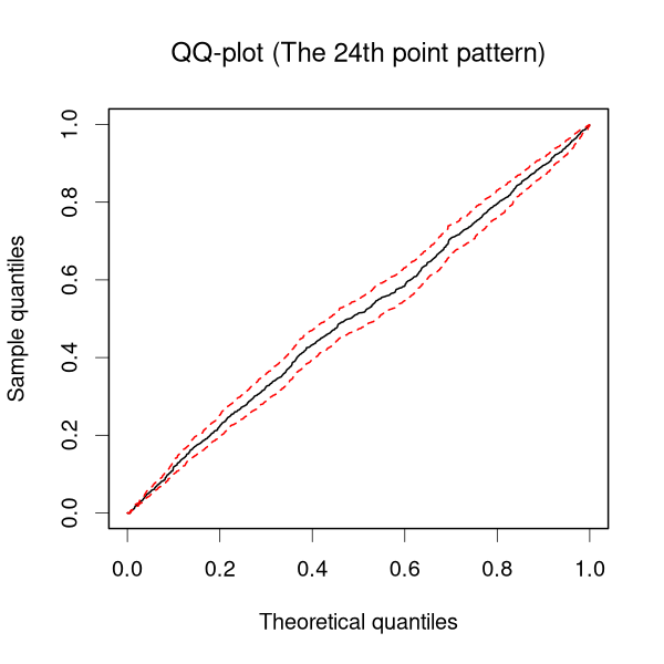
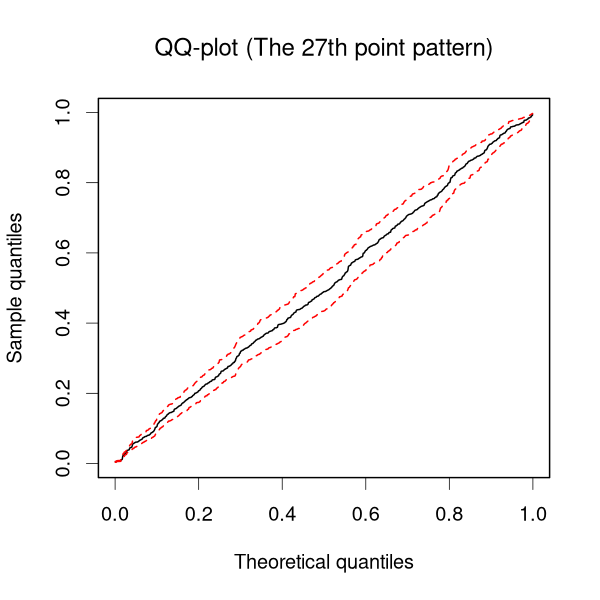
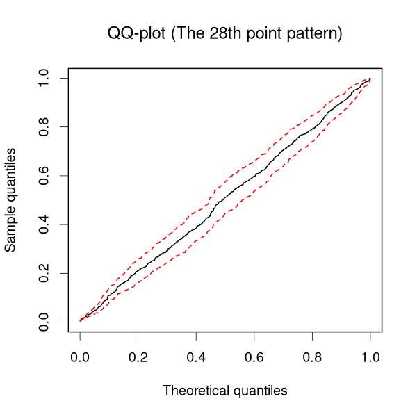
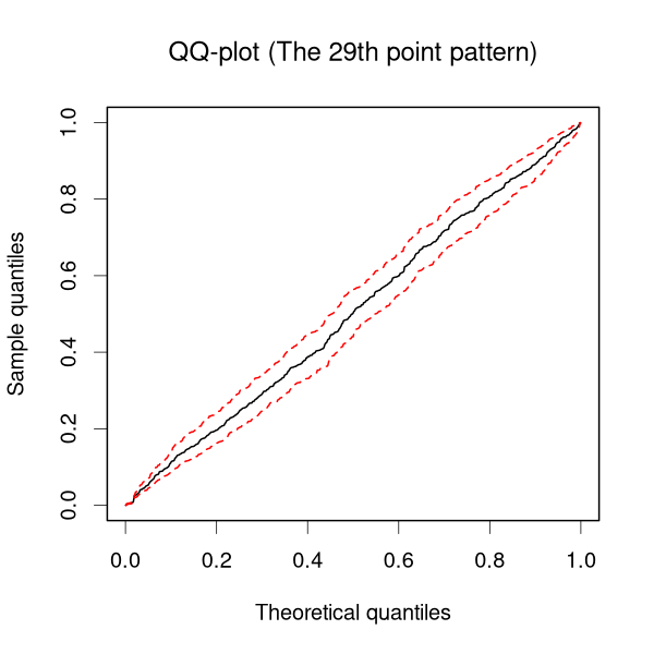
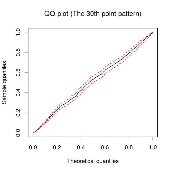
Figure S15: Model checking results for point patterns 1 - 35 in the second real data example in the main paper (Section 4.3). Black solid lines and red dotted lines are posterior mean and 95% credible interval estimates, respectively.

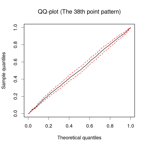
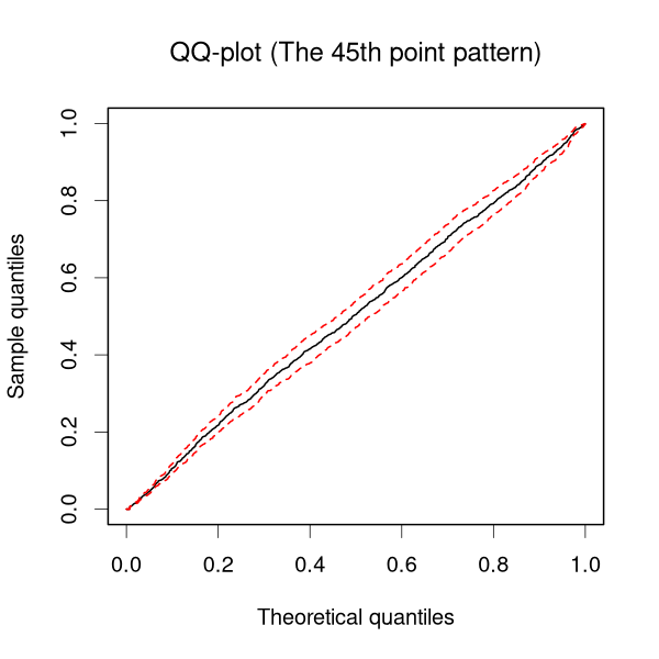
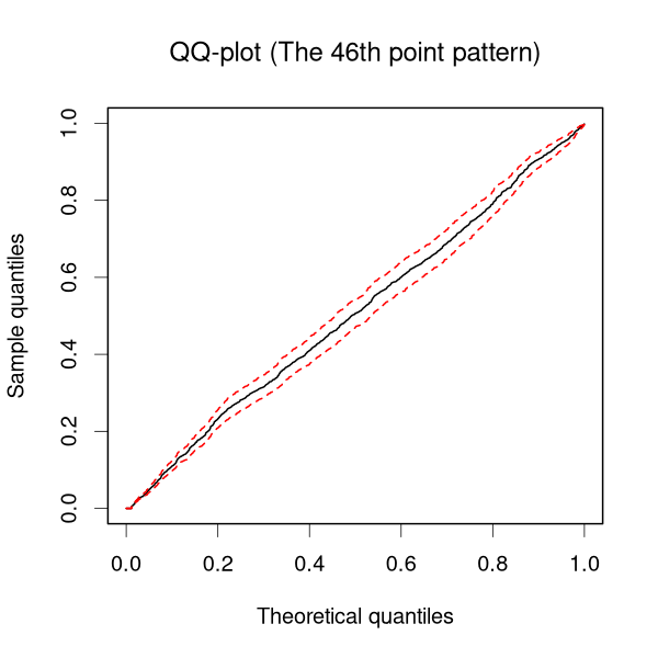
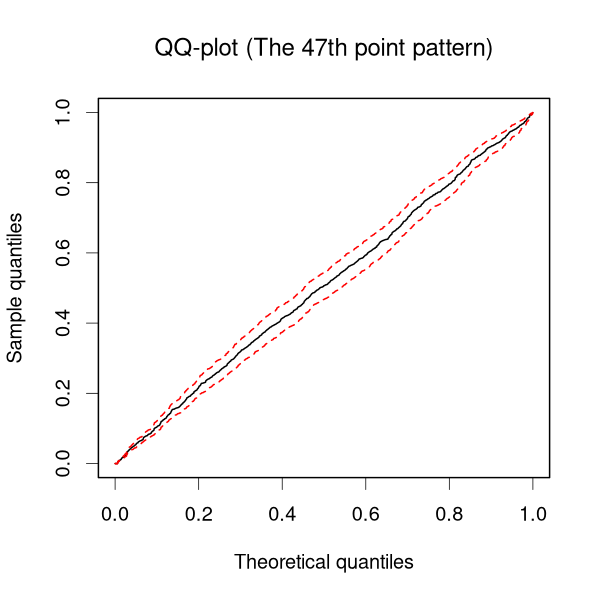
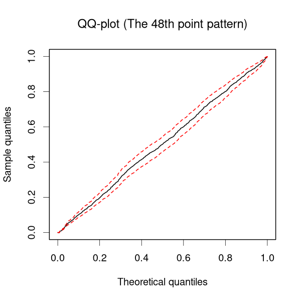
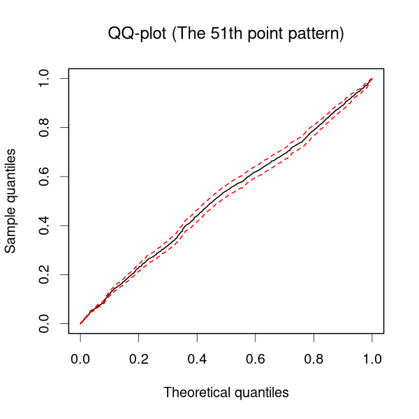
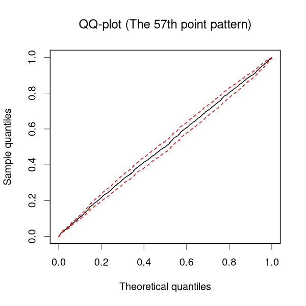
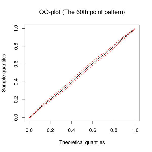
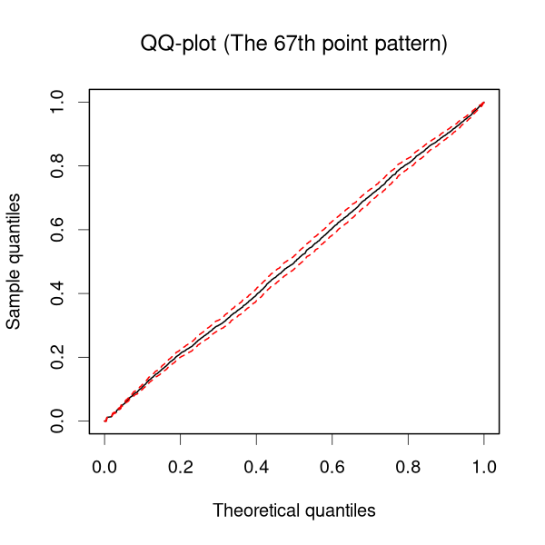
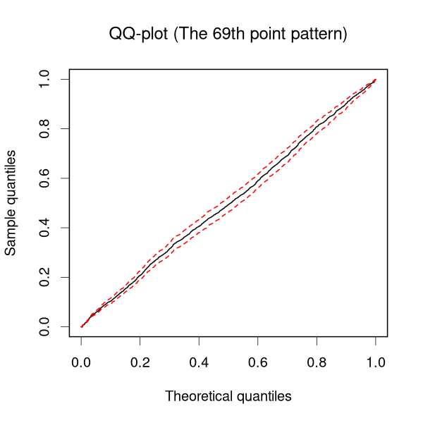
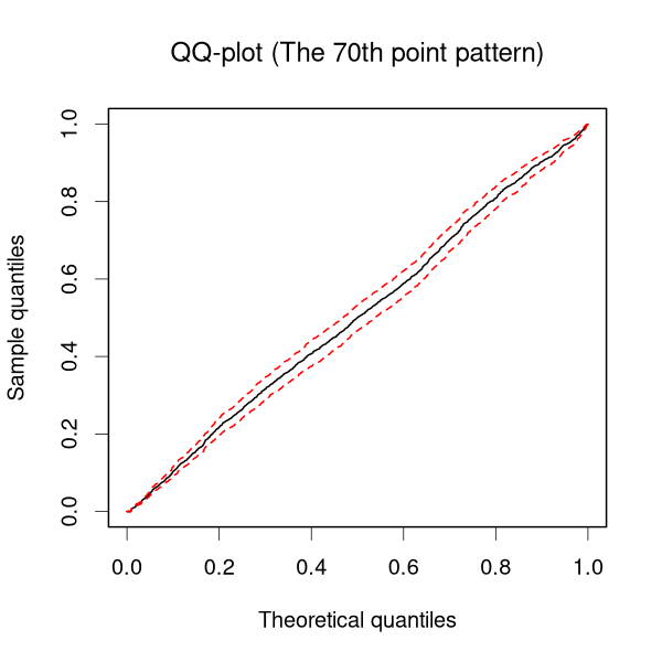
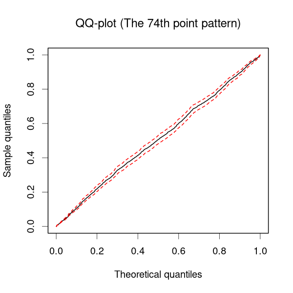
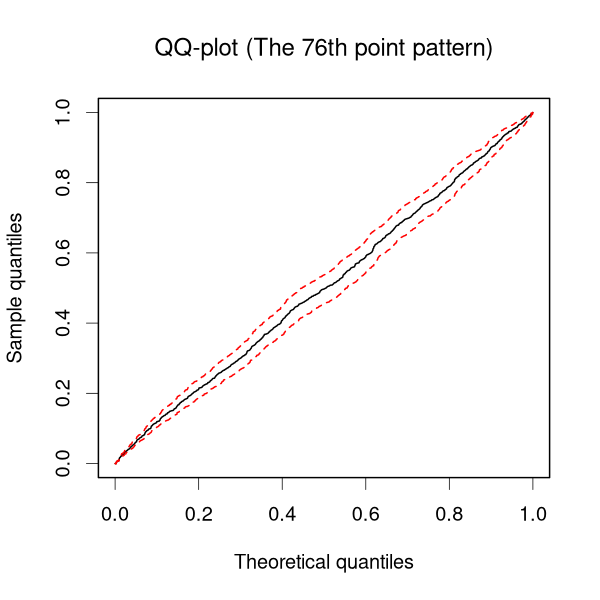
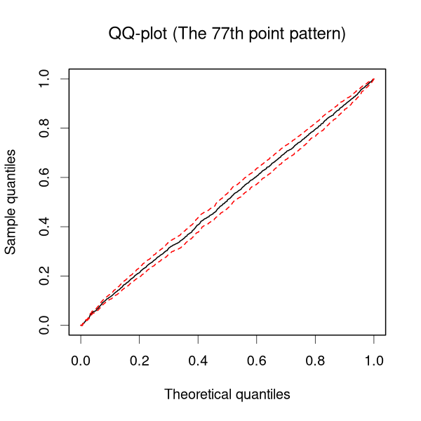
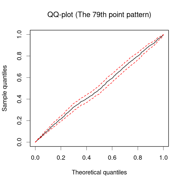
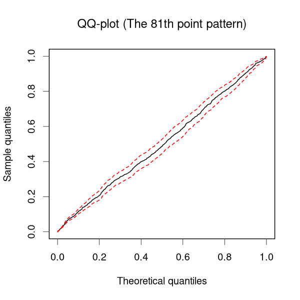
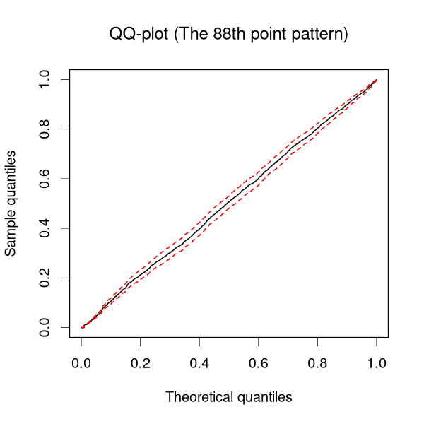
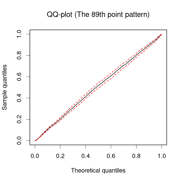
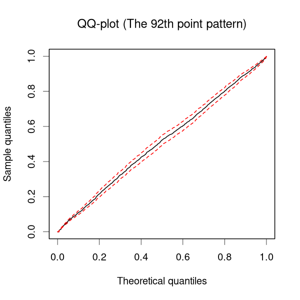
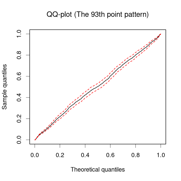
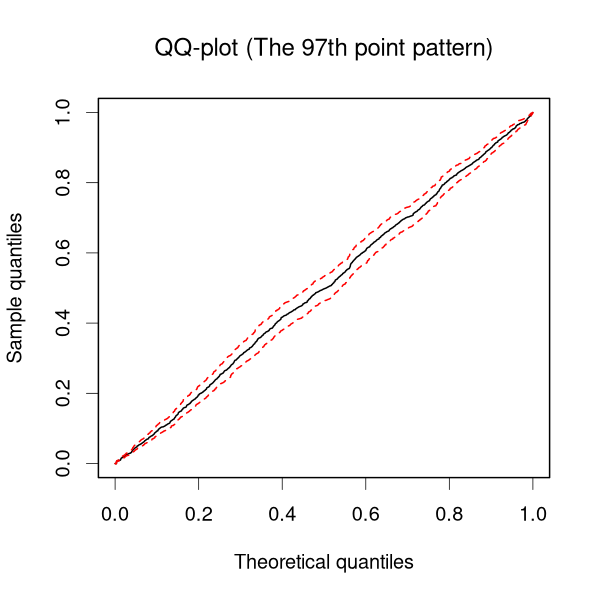
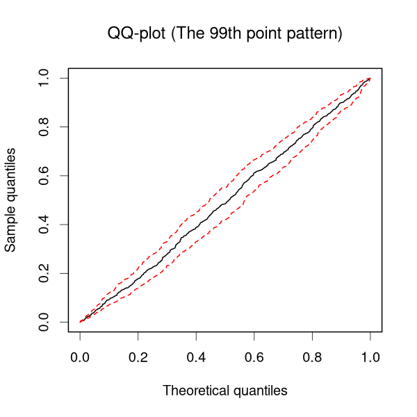
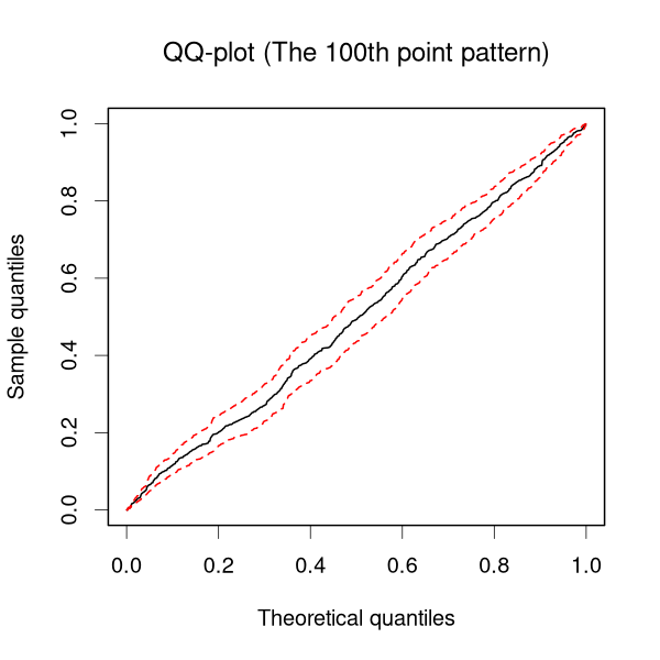
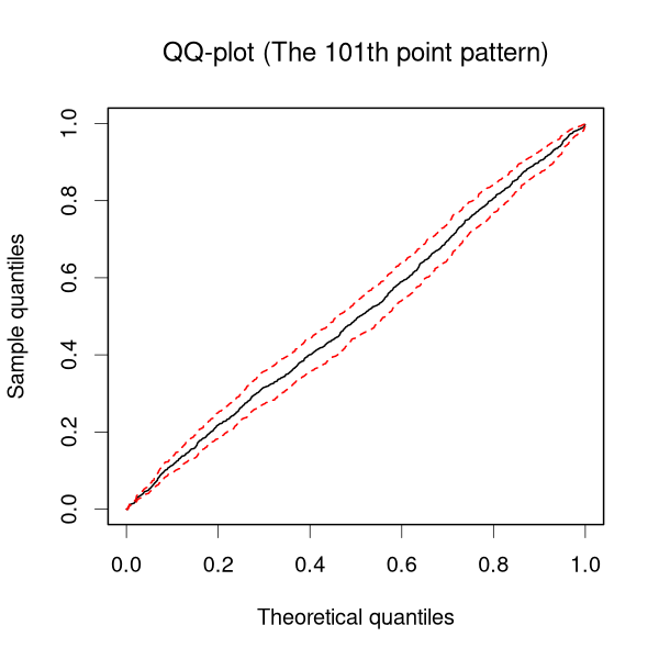
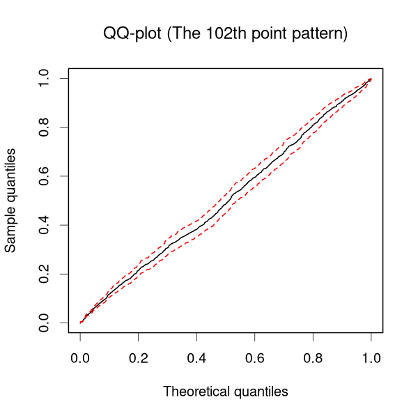
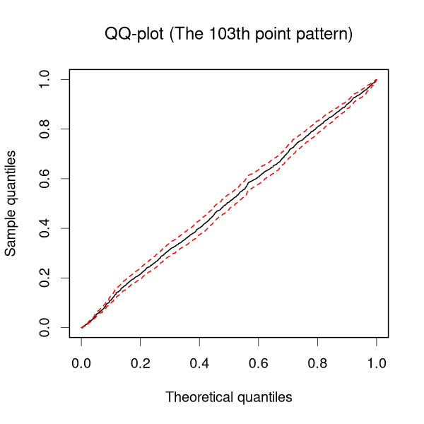
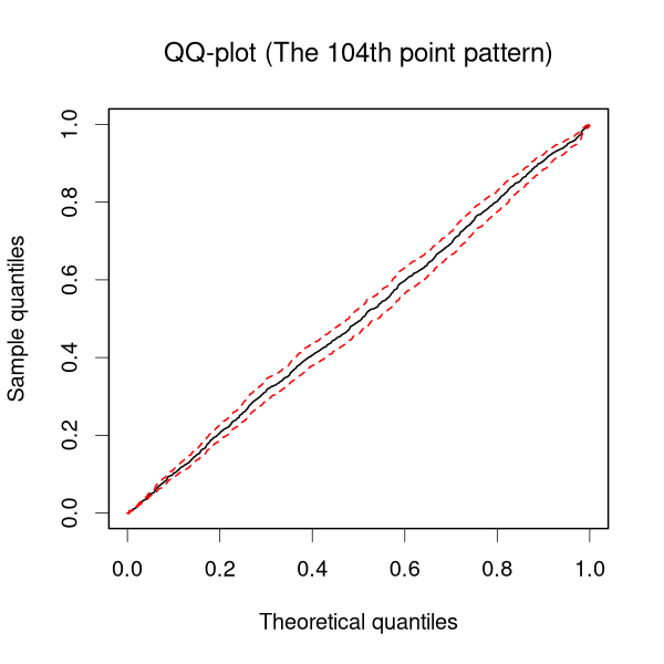
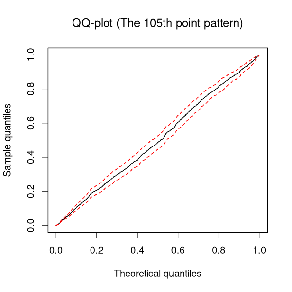
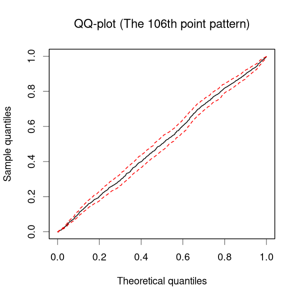
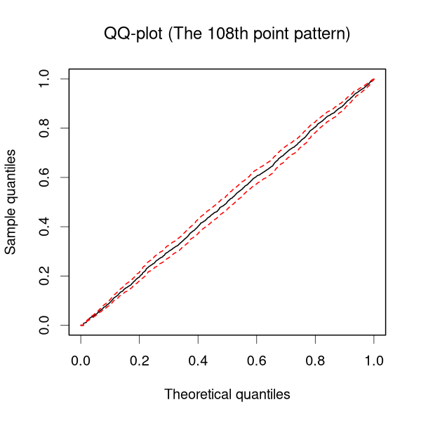
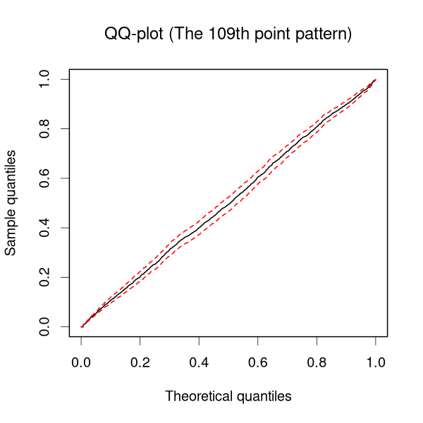
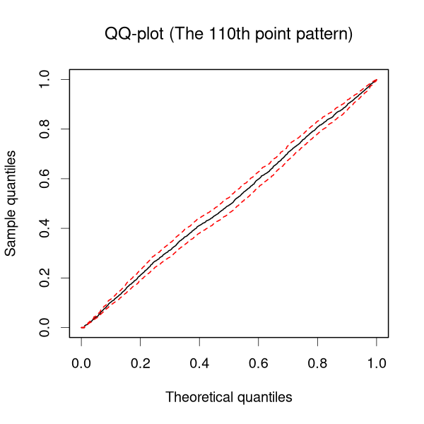
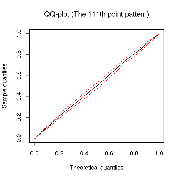
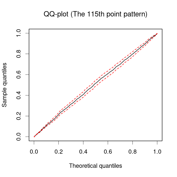
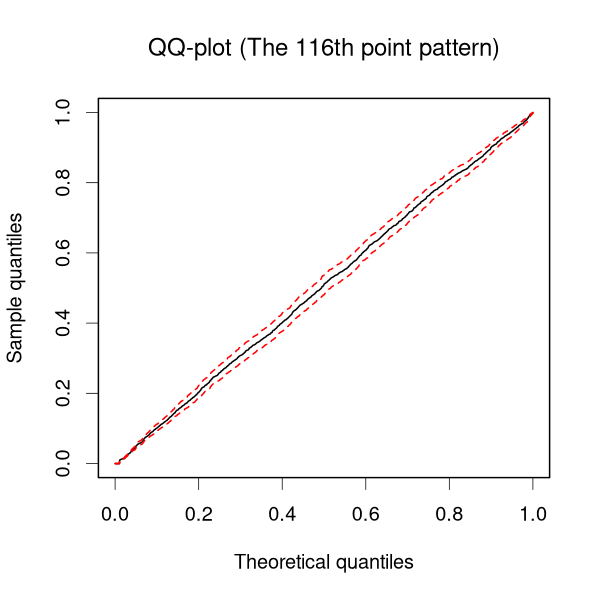
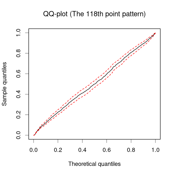
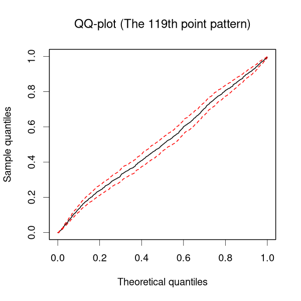
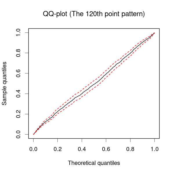
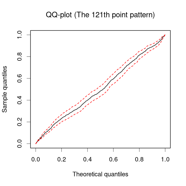
Figure S16: Model checking results for point patterns 36 - 70 in the second real data example in the main paper (Section 4.3). Black solid lines and red dotted lines are posterior mean and 95% credible interval estimates, respectively.

Figure S17: Model checking results for point patterns 71 - 105 in the second real data example in the main paper (Section 4.3). Black solid lines and red dotted lines are posterior mean and 95% credible interval estimates, respectively.

Figure S18: Model checking results for point patterns 106 - 121 in the second real data example in the main paper (Section 4.3). Black solid lines and red dotted lines are posterior mean and 95% credible interval estimates, respectively.

References

- Arnold et al. (1999) Arnold, B. C., Castillo, E., and Sarabia, J. M. (1999), Conditional Specification of Statistical Models, New York: Springer.
- Barata et al. (2022) Barata, R., Prado, R., and Sansó, B. (2022), “Fast inference for time-varying quantiles via flexible dynamic models with application to the characterization of atmospheric rivers,” The Annals of Applied Statistics, 16, 247–271.
- Bhogal and Thekke Variyam (2019) Bhogal, S. K. and Thekke Variyam, R. (2019), “Conditional duration models for high-frequency data: a review on recent developments,” Journal of Economic Surveys, 33, 252–273.
- Cavaliere et al. (2024) Cavaliere, G., Mikosch, T., Rahbek, A., and Vilandt, F. (2024), “Tail behavior of ACD models and consequences for likelihood-based estimation,” Journal of Econometrics, 238, 105613.
- Chen and Stindl (2018) Chen, F. and Stindl, T. (2018), “Direct likelihood evaluation for the renewal Hawkes process,” Journal of Computational and Graphical Statistics, 27, 119–131.
- Chen and Stindl (2022) — (2022), RHawkes: Renewal Hawkes Process. R package version 1.0.
- Coen et al. (2019) Coen, A., Gutiérrez, L., and Mena, R. H. (2019), “Modelling failures times with dependent renewal type models via exchangeability,” Statistics, 53, 1112–1130.
- Cook et al. (2007) Cook, R. J., Lawless, J. F., et al. (2007), The Statistical Analysis of Recurrent Events, New York: Springer.
- Corral (2004) Corral, Á. (2004), “Long-term clustering, scaling, and universality in the temporal occurrence of earthquakes,” Physical Review Letters, 92, 108501.
- Cowpertwait (2001) Cowpertwait, P. S. (2001), “A renewal cluster model for the inter-arrival times of rainfall events,” International Journal of Climatology, 21, 49–61.
- Daley and Vere-Jones (2003) Daley, D. J. and Vere-Jones, D. (2003), An Introduction to the Theory of Point Processes: Volume I: Elementary Theory and Methods, New York: Springer.
- Engle and Russell (1998) Engle, R. F. and Russell, J. R. (1998), “Autoregressive conditional duration: a new model for irregularly spaced transaction data,” Econometrica, 1127–1162.
- Ferguson (1973) Ferguson, T. S. (1973), “A Bayesian analysis of some nonparametric problems,” The Annals of Statistics, 209–230.
- Filimonov and Sornette (2012) Filimonov, V. and Sornette, D. (2012), “Quantifying reflexivity in financial markets: Toward a prediction of flash crashes,” Physical Review E, 85, 056108.
- Gaver and Lewis (1980) Gaver, D. P. and Lewis, P. (1980), “First-order autoregressive gamma sequences and point processes,” Advances in Applied Probability, 12, 727–745.
- Gelman et al. (2013) Gelman, A., Stern, H. S., Carlin, J. B., Dunson, D. B., Vehtari, A., and Rubin, D. B. (2013), Bayesian Data analysis, New York: Chapman and Hall/CRC, third edition.
- Grammig and Maurer (2000) Grammig, J. and Maurer, K.-O. (2000), “Non-monotonic hazard functions and the autoregressive conditional duration model,” The Econometrics Journal, 3, 16–38.
- Hassan and El-Bassiouni (2013) Hassan, M. Y. and El-Bassiouni, M. Y. (2013), “Modelling Poisson marked point processes using bivariate mixture transition distributions,” Journal of Statistical Computation and Simulation, 83, 1440–1452.
- Hassan and Lii (2006) Hassan, M. Y. and Lii, K.-S. (2006), “Modeling marked point processes via bivariate mixture transition distribution models,” Journal of the American Statistical Association, 101, 1241–1252.
- Hautsch (2011) Hautsch, N. (2011), Econometrics of Financial High-Frequency Data, New York: Springer Science & Business Media.
- Hawkes (1971) Hawkes, A. G. (1971), “Point spectra of some mutually exciting point processes,” Journal of the Royal Statistical Society: Series B (Methodological), 33, 438–443.
- Jacobs and Lewis (1977) Jacobs, P. and Lewis, P. (1977), “A mixed autoregressive-moving average exponential sequence and point process (EARMA 1, 1),” Advances in Applied Probability, 9, 87–104.
- Jiang et al. (2018) Jiang, Z.-Q., Wang, G.-J., Canabarro, A., Podobnik, B., Xie, C., Stanley, H. E., and Zhou, W.-X. (2018), “Short term prediction of extreme returns based on the recurrence interval analysis,” Quantitative Finance, 18, 353–370.
- Kottas and Sansó (2007) Kottas, A. and Sansó, B. (2007), “Bayesian mixture modeling for spatial Poisson process intensities, with applications to extreme value analysis,” Journal of Statistical Planning and Inference, 137, 3151–3163.
- Le et al. (1996) Le, N. D., Martin, R. D., and Raftery, A. E. (1996), “Modeling flat stretches, bursts outliers in time series using mixture transition distribution models,” Journal of the American Statistical Association, 91, 1504–1515.
- Modarres et al. (2017) Modarres, M., Kaminskiy, M. P., and Krivtsov, V. (2017), Reliability Engineering and Risk Analysis: A Practical Guide, Boca Raton: CRC Press.
- Ogata (1988) Ogata, Y. (1988), “Statistical models for earthquake occurrences and residual analysis for point processes,” Journal of the American Statistical Association, 83, 9–27.
- O’Hara (1995) O’Hara, M. (1995), Market Microstructure Theory, London: Blackwell.
- Pacurar (2008) Pacurar, M. (2008), “Autoregressive conditional duration models in finance: a survey of the theoretical and empirical literature,” Journal of Economic Surveys, 22, 711–751.
- Rutz et al. (2019) Rutz, J. J., Shields, C. A., Lora, J. M., Payne, A. E., Guan, B., Ullrich, P., O’brien, T., Leung, L. R., Ralph, F. M., Wehner, M., et al. (2019), “The atmospheric river tracking method intercomparison project (ARTMIP): quantifying uncertainties in atmospheric river climatology,” Journal of Geophysical Research: Atmospheres, 124, 13777–13802.
- Santhanam and Kantz (2008) Santhanam, M. and Kantz, H. (2008), “Return interval distribution of extreme events and long-term memory,” Physical Review E, 78, 051113.
- Sklar (1959) Sklar, M. (1959), “Fonctions de repartition an dimensions et leurs marges,” Publications de l’Institut de Statistique de L’Université de Paris, 8, 229–231.
- Strickland et al. (2006) Strickland, C. M., Forbes, C. S., and Martin, G. M. (2006), “Bayesian analysis of the stochastic conditional duration model,” Computational Statistics & Data Analysis, 50, 2247–2267.
- Tang and Li (2021) Tang, X. and Li, L. (2021), “Multivariate temporal point process regression,” Journal of the American Statistical Association, 1–16.
- Veen and Schoenberg (2008) Veen, A. and Schoenberg, F. P. (2008), “Estimation of space–time branching process models in seismology using an EM–type algorithm,” Journal of the American Statistical Association, 103, 614–624.
- Wheatley et al. (2016) Wheatley, S., Filimonov, V., and Sornette, D. (2016), “The Hawkes process with renewal immigration & its estimation with an EM algorithm,” Computational Statistics & Data Analysis, 94, 120–135.
- Wold (1948) Wold, H. (1948), “On stationary point processes and Markov chains,” Scandinavian Actuarial Journal, 1948, 229–240.
- Yang et al. (2018) Yang, C., Delcher, C., Shenkman, E., and Ranka, S. (2018), “Clustering inter-arrival time of health care encounters for high utilizers,” in 2018 IEEE 20th International Conference on e-Health Networking, Applications and Services (Healthcom), IEEE.
- Zheng et al. (2022) Zheng, X., Kottas, A., and Sansó, B. (2022), “On construction and estimation of stationary mixture transition distribution models,” Journal of Computational and Graphical Statistics, 31, 283–293.