Monolithic convex limiting and implicit pseudo-time stepping for calculating steady-state solutions of the Euler equations

Abstract

In this work, we use the monolithic convex limiting (MCL) methodology to enforce relevant inequality constraints in implicit finite element discretizations of the compressible Euler equations. In this context, preservation of invariant domains follows from positivity preservation for intermediate states of the density and internal energy. To avoid spurious oscillations, we additionally impose local maximum principles on intermediate states of the density, velocity components, and specific total energy. For the backward Euler time stepping, we show the invariant domain preserving (IDP) property of the fully discrete MCL scheme by constructing a fixed-point iteration that is IDP and converges under a strong time step restriction. Our iterative solver for the nonlinear discrete problem employs a more efficient fixed-point iteration. The matrix of the associated linear system is a robust low-order Jacobian approximation that exploits the homogeneity property of the flux function. The limited antidiffusive terms are treated explicitly. We use positivity preservation as a stopping criterion for nonlinear iterations. The first iteration yields the solution of a linearized semi-implicit problem. This solution possesses the discrete conservation property but is generally not IDP. Further iterations are performed if any non-IDP states are detected. The existence of an IDP limit is guaranteed by our analysis. To facilitate convergence to steady-state solutions, we perform adaptive explicit underrelaxation at the end of each time step. The calculation of appropriate relaxation factors is based on an approximate minimization of nodal entropy residuals. The performance of proposed algorithms and alternative solution strategies is illustrated by the convergence history for standard two-dimensional test problems.

1 Introduction

Recent years have witnessed significant advances in the development of bound-preserving schemes for the Euler equations of gas dynamics. In particular, flux-corrected transport (FCT) algorithms that ensure nonnegativity of continuous finite element approximations to the density and pressure (internal energy) were proposed in [9, 17, 29, 34]. A potential drawback of these explicit predictor-corrector approaches is the fact that they require the use of small time steps and do not converge to steady-state solutions. The implicit algebraic flux correction schemes employed by Gurris et al. [20] do not have this limitation. However, positivity preservation is not guaranteed even for converged solutions.

The monolithic convex limiting (MCL) methodology introduced in [26] supports the use of general time integrators. The residuals of nonlinear discrete problems are well defined both for individual time steps and for a steady-state limit. If time marching is performed using an explicit strong stability (SSP) preserving Runge–Kutta method [16], the invariant domain preservation (IDP) property of Shu–Osher stages can easily be shown following the analysis of FCT-type convex limiting approaches in [17]. The analysis of implicit MCL schemes for linear advection equations can be performed using the theoretical framework developed in [6, 32]. So far, no formal proof of the IDP property was provided for implicit MCL discretizations of the Euler equations. We fill this gap in the present paper by applying the Banach theorem to a fixed-point iteration that we design to be IDP and show to be contractive.

Having established the existence of an IDP solution to our nonlinear discrete problem, we discuss ways to calculate it in practice. Building on our previous experience with the design of iterative solvers for flux-limited finite element discretizations of the Euler system [20, 28], we update intermediate solutions using a low-order approximation to the Jacobian. The underlying linearization of nodal fluxes was proposed by Dolejšı and Feistauer [10], who performed a single iteration per time step. In our solver, we perform as many iterations as it takes to obtain a positivity-preserving result. That is, we use the IDP property as a natural stopping criterion. Another highlight of the proposed approach is a new kind of explicit underrelaxation for solution changes. We select relaxation factors from a discrete set and choose the value that corresponds to the minimum entropy residual. This selection criterion was inspired by the work of Ranocha et al. [38] on relaxation Runge–Kutta methods that ensure fully discrete entropy stability for time-dependent nonlinear problems. In our numerical studies, convergence is achieved for CFL numbers as high as $10^{5}$ and Mach numbers as high as 20.

The remainder of this article is organized as follows. We present the low-order component of our implicit MCL scheme in Section 2 and prove its IDP property in Section 3. The proof admits a straightforward generalization to the sequential MCL algorithm that we review in Section 4. The construction of the low-order Jacobian, our IDP stopping criterion for fixed-point iterations, and the adaptive choice of relaxation parameters for steady-state computations are discussed in Section 5. We present the results of our numerical experiments in Section 6 and draw conclusions in Section 7.

2 Low-order space discretization

The Euler equations of gas dynamics are a nonlinear hyperbolic system that can be written as

$$\frac{\partial u}{\partial t}+\nabla\cdot\mathbf{f}(u)=0.$$ (1)

We denote by $u=u(\mathbf{x},t)\in\mathbb{R}^{m}$, $m=d+2$ the vector of conserved quantities at a space location $\mathbf{x}\in\Omega\subset\mathbb{R}^{d},\,d\in\{1,2,3\}$ and time $t\geq 0$. The conservative variables that constitute

$$u=(\rho,\rho\mathbf{v},\rho E)^{\top}$$

are the density, momentum, and total energy, respectively. The flux function is defined by

$$\mathbf{f}(u)=(f_{1}(u),\ldots,f_{d}(u))=\left(\begin{array}[]{c}\rho\mathbf{v}^{\top}\\ \rho\mathbf{v}\otimes\mathbf{v}+pI_{d}\\ (\rho E+p)\mathbf{v}^{\top}\end{array}\right)\in\mathbb{R}^{m\times d},$$

where $I_{d}\in\mathbb{R}^{d\times d}$ is the identity tensor and $p$ is the pressure. We use the equation of state

$$p=p(u)=(\gamma-1)\biggl{(}\rho E-\frac{|\rho\mathbf{v}|^{2}}{2\rho}\biggr{)}$$

of an ideal gas with adiabatic constant $\gamma>1$. The set of physically admissible states

$$\mathcal{G}=\{u\in\mathbb{R}^{m}:\rho\geq 0,\ p\geq 0\}$$ (2)

represents an invariant domain of the Euler system  [17, 18]. A numerical method is called invariant domain preserving (IDP) or positivity preserving if it produces approximations that stay in $\mathcal{G}$.

Let us also define the Jacobians that we need to construct the matrices of our implicit finite element schemes. The array of $d$ flux Jacobians associated with the components of $\mathbf{f}(u)$ is given by

$$\mathbf{A}(u)=(A_{1}(u),\ldots,A_{d}(u))=\left(\frac{\partial f_{1}(u)}{\partial u},\ldots,\frac{\partial f_{d}(u)}{\partial u}\right)\in\mathbb{R}^{m\times m\times d}.$$

In the two-dimensional case, $\mathbf{A}(u)$ consists of [11, 19]

$$A_{1}(u)=\left(\begin{matrix}0&1&0&0\\ b_{2}v_{1}^{2}+b_{1}v_{2}^{2}&(3-\gamma)v_{1}&(1-\gamma)v_{2}&\gamma-1\\ -v_{1}v_{2}&v_{2}&v_{1}&0\\ b_{1}(v_{1}^{3}+v_{2}^{2}v_{1})-(E+\frac{p}{\rho})v_{1}&(E+\frac{p}{\rho})-(\gamma-1)v_{1}^{2}&(\gamma-1)v_{1}v_{2}&\gamma v_{1}\end{matrix}\right)$$

and

$$A_{2}(u)=\left(\begin{matrix}0&0&1&0\\ -v_{1}v_{2}&v_{2}&v_{1}&0\\ b_{2}v_{2}^{2}+b_{1}v_{1}^{2}&(1-\gamma)v_{1}&(3-\gamma)v_{2}&\gamma-1\\ b_{1}(v_{1}^{2}v_{2}+v_{2}^{3})-(E+\frac{p}{\rho})v_{2}&(\gamma-1)v_{1}v_{2}&(E+\frac{p}{\rho})-(\gamma-1)v_{2}^{2}&\gamma v_{2}\end{matrix}\right),$$

where

$$b_{1}=\frac{\gamma-1}{2},\quad b_{2}=\frac{\gamma-3}{2}.$$

For any vector $\mathbf{n}=(n_{1},\ldots,n_{d})$, the directional Jacobian

$$\mathbf{n}\cdot\mathbf{A}(u)=\sum_{i=1}^{d}n_{i}A_{i}(u)\in\mathbb{R}^{m\times m}$$

is diagonalizable. Its real eigenvalues are given by [11, 21]

$$\lambda_{1}=\mathbf{v}\cdot\mathbf{n}-c,\quad\lambda_{2}=\ldots=\lambda_{d+1}=\mathbf{v}\cdot\mathbf{n},\quad\lambda_{m}=\mathbf{v}\cdot\mathbf{n}+c,$$

where $c=c(u)=\sqrt{\frac{\gamma p}{\rho}}$ is the local speed of sound. The spectral radius

$$\lambda(u,\mathbf{n})=|\mathbf{v}\cdot\mathbf{n}|+c=\mathrm{spr}(\mathbf{n}\cdot\mathbf{A}(u))$$

of $\mathbf{n}\cdot\mathbf{A}(u)$ determines the maximum local speed of wave propagation.

Multiplying (1) by a test function $w$ and integrating over $\Omega$, we obtain the weak form

$$\int_{\Omega}w\left(\frac{\partial u}{\partial t}+\nabla\cdot\mathbf{f}(u)\right)\,\mathrm{d}\mathbf{x}=\int_{\Gamma}w(\mathbf{f}(u)\cdot\mathbf{n}-f_{n}(u,\hat{u})),$$ (3)

where $f_{n}(u,\hat{u})$ is a numerical approximation to $\mathbf{f}(u)\cdot\mathbf{n}$ depending on the external state $\hat{u}$ of the boundary condition that we impose on $\Gamma=\partial\Omega$ in a weak sense.

To begin, we discretize (3) in space using the standard continuous Galerkin (CG) method on a conforming mesh $\mathcal{T}_{h}=\{K_{1},\ldots,K_{E_{h}}\}$ consisting of $E_{h}\in\mathbb{N}$ cells. We assume that $\cup_{K\in\mathcal{T}_{h}}K\approx\overline{\Omega}$ and approximate $u$ using (multi-)linear Lagrange finite elements. The corresponding basis functions $\varphi_{1},\ldots,\varphi_{N_{h}}$ are associated with the vertices $\mathbf{x}_{1},\ldots,\mathbf{x}_{N_{h}}$ of $\mathcal{T}_{h}$ and have the property that

$$\varphi_{i}(\mathbf{x}_{j})=\delta_{ij}\quad\forall i,j\in\{1,\ldots,N_{h}\}.$$

We denote by $\mathcal{E}_{i}$ the set of indices of mesh cells containing the vertex $\mathbf{x}_{i}$. The notation

$$\mathcal{N}_{i}=\{j\in\{1,\ldots,N_{h}\}:\mathrm{supp}(\varphi_{i})\cap\mathrm{supp}(\varphi_{j})\not=\emptyset\},\qquad\mathcal{N}_{i}^{*}=\mathcal{N}_{i}\setminus\{i\}$$

is used for nodal stencils. Substituting the finite element approximations [14]

$$u_{h}=\sum_{j=1}^{N_{h}}u_{j}\varphi_{j},\quad\mathbf{f}_{h}(u_{h})=\sum_{j=1}^{N_{h}}\mathbf{f}_{j}\varphi_{j},\quad\mathbf{f}_{j}=\mathbf{f}(u_{j})$$

into (3) and using $w=\varphi_{i}$ as a test function, we obtain the standard CG discretization [26, 27]

$$\sum_{j\in\mathcal{N}_{i}}m_{ij}\frac{\mathrm{d}u_{j}}{\mathrm{d}t}=b_{i}(u_{h},\hat{u})-\sum_{j\in\mathcal{N}_{i}}\mathbf{f}_{j}\cdot\mathbf{c}_{ij},$$ (4)

where

$$m_{ij}=\sum_{e\in\mathcal{E}_{i}\cap\mathcal{E}_{j}}\int_{K_{e}}\varphi_{i}\varphi_{j}\,\mathrm{d}\mathbf{x},\qquad\mathbf{c}_{ij}=\sum_{e\in\mathcal{E}_{i}\cap\mathcal{E}_{j}}\int_{K_{e}}\varphi_{i}\nabla\varphi_{j}\,\mathrm{d}\mathbf{x},$$

$$b_{i}(u_{h},\hat{u})=\sum_{e\in\mathcal{E}_{i}}\int_{K^{e}\cap\Gamma}\varphi_{i}[\mathbf{f}(u_{h})\cdot\mathbf{n}-f_{n}(u_{h},\hat{u})]\,\mathrm{d}\mathbf{s}.$$

To construct a low-order IDP approximation, we modify (4) using the framework of algebraic flux correction [28]. The left-hand side is approximated by $m_{i}\frac{\mathrm{d}u_{i}}{\mathrm{d}t}$, where

$$m_{i}=\sum_{j=1}^{N_{h}}m_{ij}=\sum_{e\in\mathcal{E}_{i}}\int_{K_{e}}\varphi_{i}\mathrm{d}\mathbf{x}$$

is a diagonal entry of the lumped mass matrix. On the right-hand side, we replace $b_{i}(u_{h},\hat{u})$ by [26]

$$\tilde{b}_{i}(u_{i},\hat{u})=\sum_{e\in\mathcal{E}_{i}}\int_{K^{e}\cap\Gamma}\varphi_{i}[\mathbf{f}(u_{i})\cdot\mathbf{n}-f_{n}(u_{i},\hat{u}(\mathbf{x}_{i}))]\,\mathrm{d}\mathbf{s}.$$

Owing to the partition of unity property $\sum_{i}\varphi_{i}\equiv 1$ of the Lagrange basis functions, we have

$$\sum_{j\in\mathcal{N}_{i}}\mathbf{f}_{j}\cdot\mathbf{c}_{ij}=\sum_{j\in\mathcal{N}_{i}^{*}}(\mathbf{f}_{j}-\mathbf{f}_{i})\cdot\mathbf{c}_{ij}.$$

Finally, the addition of diffusive fluxes $d_{ij}(u_{j}-u_{i})$ yields the low-order scheme [17, 18, 26, 27]

$$\begin{split}m_{i}\frac{\mathrm{d}u_{i}}{\mathrm{d}t}&=\tilde{b}_{i}(u_{i},\hat{u})+\sum_{j\in\mathcal{N}_{i}^{*}}[d_{ij}(u_{j}-u_{i})-(\mathbf{f}_{j}-\mathbf{f}_{i})\cdot\mathbf{c}_{ij}]\\ &=\tilde{b}_{i}(u_{i},\hat{u})+\sum_{j\in\mathcal{N}_{i}^{*}}2d_{ij}(\overline{u}_{ij}-u_{i}),\end{split}$$ (5)

where

$$\overline{u}_{ij}=\frac{u_{j}+u_{i}}{2}-\frac{(\mathbf{f}_{j}-\mathbf{f}_{i})\cdot\mathbf{c}_{ij}}{2d_{ij}}$$

are the so-called bar states. To prove the IDP property as in [18], the graph viscosity coefficients

$$d_{ij}=\begin{cases}\max\{\lambda_{ij}|\mathbf{c}_{ij}|,\lambda_{ji}|\mathbf{c}_{ji}|\}&\text{if }j\in\mathcal{N}_{i}^{*},\\ -\sum_{k\in\mathcal{N}_{i}^{*}}d_{ik}&\text{if }j=i,\\ 0&\text{otherwise}\end{cases}$$ (6)

should be defined using a guaranteed upper bound $\lambda_{ij}$ for the maximum local wave speed of the one-dimensional Riemann problem with initial states $u_{i}$ and $u_{j}$. In the case of the Euler equations, positivity preservation can also be shown for the Rusanov wave speed [30]

$$\lambda_{ij}=\max\{|\mathbf{v}_{i}\cdot\mathbf{n}_{ij}|+c_{i},|\mathbf{v}_{j}\cdot\mathbf{n}_{ij}|+c_{j}\},$$

where $\mathbf{n}_{ij}=\frac{\mathbf{c}_{ij}}{|\mathbf{c}_{ij}|}$ is the direction of wave propagation. We use this definition of $\lambda_{ij}$ in practice.

3 Backward Euler time discretization

If the ordinary differential equation (5) is discretized in time using an explicit SSP Runge–Kutta method [16], the IDP property of each update can be shown as in [18]. In this work, our main interest is in steady-state solutions, which we calculate using pseudo-time stepping of backward Euler type. This choice allows us to use large pseudo-time steps, but we need to show the existence of an IDP solution to the resulting nonlinear system and design a robust iterative solver. We begin with the former task and prove the IDP property of the fully implicit low-order scheme in this section.

For simplicity, we assume that periodic boundary conditions are prescribed on $\Gamma$. In this case, $\tilde{b}_{i}(u_{i},\hat{u})=0$ for $i=1,\ldots,N_{h}$, and the backward Euler time discretization of (5) yields

$$u_{i}^{n+1}=u_{i}^{n}+\frac{\Delta t}{m_{i}}\sum_{j\in\mathcal{N}_{i}^{*}}2d_{ij}(\overline{u}_{ij}^{n+1}-u_{i}^{n+1}),\qquad i=1,\ldots,N_{h},$$ (7)

where $d_{ij}=d_{ij}(u^{n+1})$. We assume that there exists a finite global upper bound $\lambda>0$ for the maximum local wave speeds $\lambda_{ij}$ that are used in the definition (6) of the coefficients $d_{ij}$. It follows that

$$d_{ij}\leq\max\{|\mathbf{c}_{ij}|,|\mathbf{c}_{ji}|\}\lambda\quad\forall j\in\mathcal{N}_{i}^{*}.$$ (8)

Let $G:=\{u\in\mathbb{R}^{mN_{h}}\,:\,u_{i}\in\mathcal{G},\ i=1,\ldots,N_{h}\}$, where $\mathcal{G}$ is the invariant domain defined by (2). We claim that a solution $u=u^{n+1}$ of the nonlinear system (7) has the property that

$$u^{n}\in G\quad\Rightarrow\quad u\in G.$$

To prove the validity of this claim, we will construct a mapping $\Psi:G\mapsto G$ that is contractive under a CFL-like condition. Then we will apply Banach’s fixed-point theorem to show that

$$u=\Psi(u)\in G.$$

Following the analysis of implicit schemes in [7, 41] and adapting it to (7), we use a parameter $s>0$ to define the $i$th component of the vector $\Psi^{s}(u)$ as follows:

$$\Psi^{s}_{i}(u)=\frac{su_{i}^{n}}{1+s}+\frac{1}{1+s}\biggl{(}u_{i}+\frac{s\Delta t}{m_{i}}\sum_{j\in\mathcal{N}^{*}_{i}}2d_{ij}(\overline{u}_{ij}-u_{i})\biggr{)}=\frac{su_{i}^{n}}{1+s}+\frac{\gamma_{i}(u)}{1+s},$$

where

$$\gamma_{i}(u)=\biggl{(}1-\frac{s\Delta t}{m_{i}}\sum_{j\in\mathcal{N}^{*}_{i}}2d_{ij}\biggr{)}u_{i}+\frac{s\Delta t}{m_{i}}\sum_{j\in\mathcal{N}^{*}_{i}}2d_{ij}\overline{u}_{ij}.$$

Note that $\Psi^{s}_{i}(u)$ is a convex combination of $u_{i}^{n}$ and $\gamma_{i}(u)$. The assumption that $u_{i}^{n}\in\mathcal{G}$ implies that $\Phi(u_{i}^{n})\geq 0$ for $\Phi\in\{\rho,p\}$. For any concave nonnegative function $\Phi$, we have the estimate

$$\Phi(\Psi^{s}_{i}(u))\geq\frac{s}{1+s}\Phi(u_{i}^{n})+\frac{1}{1+s}\Phi(\gamma_{i}(u))\geq\frac{1}{1+s}\Phi(\gamma_{i}(u)).$$

Furthermore, $\gamma_{i}(u)$ is a convex combination of $u_{i}$ and $\overline{u}_{ij}$ under the CFL-like condition

$$\frac{s\Delta t}{m_{i}}\sum_{j\in\mathcal{N}^{*}_{i}}2d_{ij}\leq 1.$$ (9)

This implies that

$$\Phi(\gamma_{i}(u))\geq\biggl{(}1-\frac{s\Delta t}{m_{i}}\sum_{j\in\mathcal{N}^{*}_{i}}2d_{ij}\biggr{)}\Phi(u_{i})+\frac{s\Delta t}{m_{i}}\sum_{j\in\mathcal{N}^{*}_{i}}2d_{ij}\Phi(\overline{u}_{ij}).$$

The bar states $\overline{u}_{ij}$ represent averaged exact solutions of one-dimensional Riemann problems [18]. Thus,

$$u_{i},u_{j}\in\mathcal{G}\quad\Rightarrow\quad\overline{u}_{ij}\in\mathcal{G}\quad\Rightarrow\quad\Phi(\overline{u}_{ij})\geq 0\ \mbox{for}\ \Phi\in\{\rho,p\}.$$

From this we deduce that $\Phi(\Psi^{s}_{i}(u))\geq 0$ for $\Phi\in\{\rho,p\}$ and, therefore, $\Psi^{s}(u)\in G$ for all $u\in G$.

Let us now set $u^{(0)}=u^{n}$ and use the mapping $\Psi^{s}:G\mapsto G$ to construct the fixed-point iteration

$$u^{(k+1)}=\Psi^{s}(u^{(k)}),\quad k\in\mathbb{N}_{0}.$$ (10)

It remains to check if this iteration converges to a fixed point $u=\Psi(u)$. Banach’s theorem is applicable if the mapping $\Psi^{s}$ is contractive, i.e., if there exists $L\in[0,1)$, such that

$$\|\Psi^{s}(v)-\Psi^{s}(w)\|\leq L\|v-w\|\quad\forall v,w\in G$$

for some vector norm $\|\cdot\|$. For arbitrary $v,w\in G$, we have

$$\Psi^{s}_{i}(v)-\Psi_{i}^{s}(w)= \frac{1}{1+s}\biggl{(}v_{i}-w_{i}+\frac{s\Delta t}{m_{i}}\sum_{j\in\mathcal{N}^{*}_{i}}2d_{ij}\bigl{(}(\overline{v}_{ij}-v_{i})-(\overline{w}_{ij}-w_{i})\bigr{)}\biggr{)}$$

$$= \frac{1}{1+s}\biggl{[}v_{i}-w_{i}+\frac{s\Delta t}{m_{i}}\sum_{j\in\mathcal{N}^{*}_{i}}d_{ij}\bigl{(}(v_{j}-w_{j})-(v_{i}-w_{i})\bigr{)}$$

$$-\bigl{[}\bigl{(}\mathbf{f}(v_{j})-\mathbf{f}(w_{j})\bigr{)}-\bigl{(}\mathbf{f}(v_{i})-\mathbf{f}(w_{i})\bigr{)}\bigr{]}\cdot\mathbf{c}_{ij}\biggr{]}.$$

The involved flux differences can be written in the quasi-linear incremental form [28, 39]

$$\bigl{(}\mathbf{f}(v_{j})-\mathbf{f}(w_{j})\bigr{)}\cdot\mathbf{c}_{ij}=|\mathbf{c}_{ij}|A_{ij}(v_{j}-w_{j}),$$

where $A_{ij}\coloneqq A(v_{j},w_{j};\mathbf{n}_{ij})\in\mathbb{R}^{m\times m}$ is the Roe matrix. It is known from linear algebra that for any $\varepsilon>0$ and any matrix $A\in\mathbb{R}^{m\times m}$, there exists a vector norm $\|\cdot\|_{\varepsilon}$ such that [37]

$$\|A\|_{\varepsilon}<\mathrm{spr}(A)+\varepsilon,$$

where $\|A\|_{\varepsilon}=\max_{u\not=0}\frac{\|Au\|_{\varepsilon}}{\|u\|_{\varepsilon}}$ and $\mathrm{spr}(A)$ is the spectral radius of $A$. It follows that

$$\|(\mathbf{f}(v_{j})-\mathbf{f}(w_{j}))\cdot\mathbf{c}_{ij}\|_{\varepsilon}\leq|\mathbf{c}_{ij}|\|A_{ij}\|_{\varepsilon}\|v_{j}-w_{j}\|_{\varepsilon}\leq|\mathbf{c}_{ij}|(\mathrm{spr}(A_{ij})+\varepsilon)\|v_{j}-w_{j}\|_{\varepsilon}.$$

Furthermore, the spectral radius of the Roe matrix $A_{ij}$ is bounded above by the maximum global wave speed $\lambda$ that we used in (8). Introducing the norm $\|v\|_{\infty,\varepsilon}\coloneqq\max_{1\leq i\leq N_{h}}\|v_{i}\|_{\varepsilon}$, we obtain

$$\|\Psi^{s}(v)-\Psi^{s}(w)\|_{\infty,\varepsilon}\leq \max_{1\leq i\leq N_{h}}\frac{1}{1+s}\biggl{(}\|v_{i}-w_{i}\|_{\varepsilon}+2\frac{s\Delta t}{m_{i}}\sum_{j\in\mathcal{N}_{i}^{*}}(2\lambda+\varepsilon)\max\{|\mathbf{c}_{ij}|,|\mathbf{c}_{ji}|\}\|v_{j}-w_{j}\|_{\varepsilon}\biggr{)}$$

$$\leq \max_{1\leq i\leq N_{h}}\frac{1}{1+s}\biggl{(}1+s\frac{2\Delta t}{m_{i}}\sum_{j\in\mathcal{N}_{i}^{*}}(2\lambda+\varepsilon)\max\{|\mathbf{c}_{ij}|,|\mathbf{c}_{ji}|\}\biggr{)}\|v-w\|_{\infty,\varepsilon}.$$

This estimate shows that $\{\Psi^{s}\}_{s>0}$ is a family of contractions under the CFL-like condition

$$\frac{2\Delta t}{m_{i}}\sum_{j\in\mathcal{N}_{i}^{*}}(2\lambda+\varepsilon)\max\{|\mathbf{c}_{ij}|,|\mathbf{c}_{ji}|\}<1,\quad 1\leq i\leq N_{h},$$ (11)

which is independent of the parameter $s>0$. By Banach’s theorem, the fixed-point iteration (10) converges to a unique limit $u=\Psi^{s}(u)\in G$ provided that $u^{(0)}\in G$ and condition (11) holds. Thus, we have shown the existence of a unique IDP solution to (7) under these assumptions.

4 Monolithic convex limiting

By the Godunov theorem, the spatial semi-discretization (7) is at most first-order accurate. Obviously, the accuracy of steady-state solutions is also affected by this order barrier. The monolithic convex limiting (MCL) strategy proposed in [26, 27] makes it possible to achieve higher resolution without losing the IDP property and inhibiting convergence to steady-state solutions. To explain the MCL design philosophy, we write the Galerkin space discretization (4) in the bar state form

$$m_{i}\frac{\mathrm{d}u_{i}}{\mathrm{d}t}=\tilde{b}_{i}(u_{i},\hat{u})+\sum_{j\in\mathcal{N}_{i}^{*}}2d_{ij}(\overline{u}_{ij}^{H}-u_{i}),$$

which exhibits the same structure as (5). The high-order bar states

$$\overline{u}_{ij}^{H}=\overline{u}_{ij}+\frac{f_{ij}^{H}}{2d_{ij}}$$

depend on the raw antidiffusive fluxes [26, 27]

$$f_{ij}^{H}=m_{ij}\left(\dot{u}_{i}^{H}-\dot{u}_{j}^{H}\right)+d_{ij}(u_{i}-u_{j}).$$

The high-order time derivatives $\dot{u}_{i}^{H}$ satisfy the linear system

$$\sum_{j\in\mathcal{N}_{i}}m_{ij}\dot{u}_{j}^{H}=\tilde{b}_{i}(u_{i},\hat{u})-\sum_{j\in\mathcal{N}_{i}^{*}}(\mathbf{f}_{j}-\mathbf{f}_{i})\cdot\mathbf{c}_{ij},\quad i=1,\ldots,N_{h}.$$

For efficiency and stability reasons, we replace $f_{ij}^{H}$ by the flux [26, 32]

$$f_{ij}=m_{ij}\left(\dot{u}_{i}^{L}-\dot{u}_{j}^{L}\right)+d_{ij}(u_{i}-u_{j})$$

that is defined using the low-order time derivatives

$$\dot{u}_{i}^{L}=\frac{1}{m_{i}}\left(\tilde{b}_{i}(u_{i},\hat{u})+\sum_{j\in\mathcal{N}_{i}^{*}}[d_{ij}(u_{j}-u_{i})-(\mathbf{f}_{j}-\mathbf{f}_{i})\cdot\mathbf{c}_{ij}]\right).$$

In general, we denote by $f_{ij}$ the target flux corresponding to a high-order baseline scheme. The MCL approach introduced in [26] approximates $f_{ij}=-f_{ji}$ by a limited flux $f_{ij}^{*}=-f_{ji}^{*}$ such that

$$\overline{u}_{ij},\overline{u}_{ji}\in\mathcal{G}\quad\Rightarrow\quad\overline{u}_{ij}^{*}:=\overline{u}_{ij}+\frac{f_{ij}^{*}}{2d_{ij}}\in\mathcal{G},\qquad\overline{u}_{ji}^{*}:=\overline{u}_{ji}-\frac{f_{ij}^{*}}{2d_{ij}}\in\mathcal{G}$$

and local discrete maximum principles are satisfied for some scalar quantities of interest.

In this work, we use a sequential MCL algorithm that imposes local bounds on the density, velocity, and specific total energy (as in [26, 27]). The local bounds of the density constraints

$$\rho_{i}^{\min}\leq\overline{\rho}_{ij}^{*}=\overline{\rho}_{ij}-\frac{f_{ij}^{*,\rho}}{2d_{ij}}\leq\rho_{i}^{\max}\qquad\forall j\in\mathcal{N}_{i}^{*}$$ (12)

are given by

$$\rho_{i}^{\min}=\min\left\{\min_{j\in\mathcal{N}_{i}}\rho_{j},\min_{j\in\mathcal{N}_{i}^{*}}\overline{\rho}_{ij}\right\},\qquad\rho_{i}^{\max}=\max\left\{\max_{j\in\mathcal{N}_{i}}\rho_{j},\max_{j\in\mathcal{N}_{i}^{*}}\overline{\rho}_{ij}\right\}.$$

The density constraints are satisfied by the limited antidiffusive fluxes [26, 27]

$$f_{ij}^{*,\rho}=\begin{cases}\min\{f_{ij}^{\rho},\,2d_{ij}\min\{\rho_{i}^{\max}-\overline{\rho}_{ij},\,\overline{\rho}_{ji}-\rho_{j}^{\min}\}\}\quad&\text{if }f_{ij}^{\rho}>0,\\ \max\{f_{ij}^{\rho},\,2d_{ij}\max\{\rho_{i}^{\min}-\overline{\rho}_{ij},\,\overline{\rho}_{ji}-\rho_{j}^{\max}\}\}\quad&\text{otherwise,}\end{cases}$$

where $f_{ij}^{\rho}$ is the first component of the target flux $f_{ij}\in\mathbb{R}^{m}$.

The components of $\mathbf{v}=(v_{1},\ldots,v_{d})$ and the specific total energy $E$ are derived quantities that cannot be limited directly. Instead, conserved products $\rho\phi$, where $\phi\in\{v_{1},\ldots,v_{d},E\}$, are limited using a discrete version of the product rule. Introducing the notation [27, 26]

$$\phi_{i}=\frac{(\rho\phi)_{i}}{\rho_{i}},\quad\overline{\phi}_{ij}=\frac{\overline{(\rho\phi)}_{ij}+\overline{(\rho\phi)}_{ji}}{\overline{\rho}_{ij}+\overline{\rho}_{ji}},$$

we use limited counterparts $g_{ij}^{\rho\phi,*}$ of the auxiliary fluxes

$$g_{ij}^{\rho\phi}=f_{ij}^{\rho\phi}+2d_{ij}\left[\overline{(\rho\phi)}_{ij}-\overline{\rho}_{ij}^{*}\overline{\phi}_{ij}\right]$$

to define

$$f_{ij}^{\rho\phi,*}=g_{ij}^{\rho\phi,*}-2d_{ij}\left[\overline{(\rho\phi)}_{ij}-\overline{\rho}_{ij}^{*}\overline{\phi}_{ij}\right].$$ (13)

Note that the target flux $f_{ij}^{\rho\phi}$ can be recovered using $g_{ij}^{\rho\phi,*}=g_{ij}^{\rho\phi}$. The general definition of $g_{ij}^{\rho\phi,*}$ should ensure that $f_{ij}^{\rho\phi,*}$ satisfies the local discrete maximum principle

$$\overline{\rho}_{ij}^{*}\phi_{i}^{\min}\leq\overline{(\rho\phi)}_{ij}^{*}=\overline{(\rho\phi)}_{ij}+\frac{f_{ij}^{\rho\phi,*}}{2d_{ij}}\leq\overline{\rho}_{ij}^{*}\phi_{i}^{\max}$$ (14)

with local bounds

$$\phi_{i}^{\min}=\min\left\{\min_{j\in\mathcal{N}_{i}}\phi_{j},\min_{j\in\mathcal{N}_{i}^{*}}\overline{\phi}_{ij}\right\},\quad\phi_{i}^{\max}=\max\left\{\max_{j\in\mathcal{N}_{i}}\phi_{j},\max_{j\in\mathcal{N}_{i}^{*}}\overline{\phi}_{ij}\right\}.$$ (15)

The choice $g_{ij}^{\rho\phi,*}=0$ yields the low-order bar state $\overline{(\rho\phi)}_{ij}=\overline{\rho}_{ij}^{*}\overline{\phi}_{ij}$, which satisfies (14) by (15). It is easy to verify that the constraints are also satisfied for

$$g_{ij}^{\rho\phi,*}=\begin{cases}\min\left\{g_{ij}^{\rho\phi},g_{ij}^{\rho\phi,\max}\right\}&\text{if }g_{ij}^{\rho\phi}>0,\\ \max\left\{g_{ij}^{\rho\phi},g_{ij}^{\rho\phi,\min}\right\}&\text{if }g_{ij}^{\rho\phi}\leq 0,\\ \end{cases}$$ (16)

where we use the bounding fluxes

$$\begin{split}g_{ij}^{\rho\phi,\max}&=\min\left\{2d_{ij}\overline{\rho}_{ij}^{*}(\phi_{i}^{\max}-\overline{\phi}_{ij}),2d_{ji}\overline{\rho}_{ji}^{*}(\overline{\phi}_{ji}-\phi_{i}^{\min})\right\},\\ g_{ij}^{\rho\phi,\min}&=\max\left\{2d_{ij}\overline{\rho}_{ij}^{*}(\phi_{i}^{\min}-\overline{\phi}_{ij}),2d_{ji}\overline{\rho}_{ji}^{*}(\overline{\phi}_{ji}-\phi_{i}^{\max})\right\}.\end{split}$$

The corresponding limited flux $f_{ij}^{\rho\phi,*}$ is obtained by substituting (16) into (13).

In the final step of the sequential limiting procedure, we use a scalar correction factor $\alpha_{ij}\in[0,1]$ to ensure the IDP property of the bar states

$$\bar{u}_{ij}^{*,\alpha}=\bar{u}_{ij}+\frac{\alpha_{ij}f_{ij}^{*}}{2d_{ij}},$$

where $f_{ij}^{*}=\left(f_{ij}^{\rho,*},\mathbf{f}_{ij}^{\rho\mathbf{v},*},f_{ij}^{\rho E,*}\right)^{\top}$ is the vector of prelimited fluxes. Note that $\bar{\rho}_{ij}^{*,\alpha}\geq 0$ for any $\alpha_{ij}\in[0,1]$ because the lower bounds of the density constraints (12) are nonnegative. The pressure constraint

$$p(\overline{u}_{ij}^{*,\alpha})\geq 0\quad\Leftrightarrow\quad\overline{(\rho E)}^{*,\alpha}_{ij}\geq\frac{|\overline{(\rho\mathbf{v})}^{*,\alpha}_{ij}|^{2}}{2\overline{\rho}^{*,\alpha}_{ij}}$$

is satisfied for $\alpha_{ij}\in[0,1]$ such that

$$P_{ij}(\alpha_{ij})\leq Q_{ij},$$ (17)

where

$$P_{ij}(\alpha)=\left[\frac{|\mathbf{f}_{ij}^{\rho\mathbf{v},*}|^{2}}{2}-f_{ij}^{\rho E,*}f_{ij}^{\rho,*}\right]\alpha^{2}+2d_{ij}\left[\overline{(\rho\mathbf{v})}_{ij}\cdot\mathbf{f}_{ij}^{\rho\mathbf{v},*}-\overline{\rho}_{ij}f_{ij}^{\rho E,*}-\overline{(\rho E)}_{ij}f_{ij}^{\rho,*}\right]\alpha$$

and

$$Q_{ij}=(2d_{ij})^{2}\overline{\rho}_{ij}\left[\overline{(\rho E)}_{ij}-\frac{|\overline{(\rho\mathbf{v})}_{ij}|^{2}}{2\overline{\rho}_{ij}}\right].$$

Note that $Q_{ij}\geq 0$ since $\overline{u}_{ij}\in\mathcal{G}$. Instead of maximizing $\alpha\in[0,1]$ subject to $P_{ij}(\alpha)\leq Q_{ij}$, the pressure fix proposed in [26] replaces (17) by the linear sufficient condition

$$\alpha_{ij}R_{ij}\leq Q_{ij},$$ (18)

where

$$\begin{split}R_{ij}&=\max\left\{0,2d_{ij}\left[\overline{(\rho\mathbf{v})}_{ij}\cdot\mathbf{f}_{ij}^{\rho\mathbf{v},*}-\overline{\rho}_{ij}f_{ij}^{\rho E,*}-\overline{(\rho E)}_{ij}f_{ij}^{\rho,*}\right]\right\}\\ &+\max\left\{0,\frac{|\mathbf{f}_{ij}^{\rho\mathbf{v},*}|^{2}}{2}-f_{ij}^{\rho E,*}f_{ij}^{\rho,*}\right\}.\end{split}$$

To ensure continuous dependence of the limited flux $\alpha_{ij}f_{ij}^{*}$ on the data and avoid convergence problems at steady state, we overestimate the bound $R_{ij}$ by [26, 27]

$$\begin{split}R_{ij}^{\max}&=2d_{ij}\left[\max\left\{|\overline{(\rho\mathbf{v})}_{ij}|,|\overline{(\rho\mathbf{v})}_{ji}|\right\}|\mathbf{f}_{ij}^{\rho\mathbf{v},*}|\right.\\ &\left.+\max\left\{\overline{\rho}_{ij},\overline{\rho}_{ji}\right\}|f_{ij}^{\rho E,*}|+\max\left\{\overline{(\rho E)}_{ij},\overline{(\rho E)}_{ji}\right\}|f_{ij}^{\rho,*}|\right]\\ &+\max\left\{0,\frac{|\mathbf{f}_{ij}^{\rho\mathbf{v},*}|^{2}}{2}-f_{ij}^{\rho E,*}f_{ij}^{\rho,*}\right\}=R_{ji}^{\max}\end{split}$$

but remark that this overestimation may increase the levels of artificial viscosity [40]. Taking the symmetry condition $\alpha_{ij}=\alpha_{ji}$ and the constraint $\alpha_{ji}R_{ji}\leq Q_{ji}$ into account, we apply

$$\alpha_{ij}=\begin{cases}\frac{\min(Q_{ij},Q_{ji})}{R_{ij}^{\max}}&\text{if }R_{ij}^{\max}>\min(Q_{ij},Q_{ji}),\\ 1&\text{otherwise}\end{cases}$$

to all components of the prelimited flux $f_{ij}^{*}$. This final limiting step ensures that $\overline{u}_{ij}^{*,\alpha}\in\mathcal{G}$ whenever $\overline{u}_{ij}\in\mathcal{G}$. The IDP property of the fully implicit MCL scheme

$$u_{i}^{n+1}=u_{i}^{n}+\frac{\Delta t}{m_{i}}\sum_{j\in\mathcal{N}_{i}^{*}}2d_{ij}(\overline{u}_{ij}^{*,\alpha,n+1}-u_{i}^{n+1}),\qquad i=1,\ldots,N_{h}$$ (19)

can now be shown in exactly the same manner as for the low-order method (7) in Section 3.

5 Solution of nonlinear systems

In principle, we could solve (19) using the IDP fixed-point iteration (10) with the mapping

$$\Psi^{s}_{i}(u) =\frac{su_{i}^{n}}{1+s}+\frac{1}{1+s}\biggl{(}u_{i}+\frac{s\Delta t}{m_{i}}\Big{[}\tilde{b}_{i}(u_{i},\hat{u})+\sum_{j\in\mathcal{N}^{*}_{i}}2d_{ij}(\overline{u}_{ij}^{*,\alpha}-u_{i})\Big{]}\biggr{)},\quad s>0.$$ (20)

The analysis performed in Section 3 guarantees the IDP property of intermediate solutions under condition (9), which can always be enforced by choosing a sufficiently small value of the parameter $s>0$. However, Banach’s theorem guarantees convergence only for time steps satisfying the restrictive CFL-like condition (11). Using such time steps in actual computations is clearly impractical, because explicit alternatives would be at least as efficient. Of course, there is an option of using larger time steps in practice but the convergence behavior of the simple fixed-point iteration (10) is inferior to that of the quasi-Newton / deferred correction methods to be discussed in this section.

5.1 Solver for individual time steps

The flux-corrected nonlinear system (19) can be written in the following split matrix form:

$$M_{L}u^{n+1}=M_{L}u^{n}+\Delta t[R_{L}(u^{n+1})+F^{*}(u^{n+1})].$$ (21)

We denote by $M_{L}=(\delta_{ij}m_{i}I_{m})_{i,j=1}^{N_{h}}$ the lumped mass matrix. The components of the low-order steady-state residual $R_{L}(u)$ and of the high-order correction term $F^{*}(u)$ are defined by

$$(R_{L}(u))_{i}=\tilde{b}_{i}(u_{i},\hat{u})+\sum_{j\in\mathcal{N}_{i}^{*}}[d_{ij}(u_{j}-u_{i})-(\mathbf{f}_{j}-\mathbf{f}_{i})\cdot\mathbf{c}_{ij}],\qquad F_{i}^{*}(u)=\sum_{j\in\mathcal{N}_{i}^{*}}\alpha_{ij}f_{ij}^{*}.$$

A quasi-Newton method for solving (21) uses an approximate Jacobian $J(u)$ in updates of the form

$$J(u^{(k)})(u^{(k+1)}-u^{(k)})=M_{L}(u^{n}-u^{(k)})+\Delta t[R_{L}(u^{(k)})+F^{*}(u^{(k)})],\quad k\in\mathbb{N}_{0},$$ (22)

where $u^{(k)}$ is a given approximation to $u^{n+1}$. By default, we set $u^{(0)}=u^{n}$ and use a low-order Jacobian approximation $J(u)=J_{L}(u)$, the derivation of which is explained below.

The homogeneity property $\mathbf{f}(u)=\mathbf{A}(u)u$ of the flux function of the Euler equations implies that

$$\mathbf{f}_{j}-\mathbf{f}_{i}=\mathbf{A}(u_{j})u_{j}-\mathbf{A}(u_{i})u_{i}.$$ (23)

Dolejšı and Feistauer [10] used this property to design a conservative linearized implicit scheme. Further representatives of such schemes were derived and analyzed by Kučera et al. [25]. The algorithm employed by Gurris et al. [20] is similar but provides the option of performing multiple iterations.

In view of (23), the Jacobian associated with the low-order component of (21) is given by [19]

$$J_{L}=M_{L}+\Delta t[A-B-D],$$

where $A=(A_{ij})_{i,j=1}^{N_{h}}$ and $D=(D_{ij})_{i,j=1}^{N_{h}}$ are sparse block matrices composed from

$$A_{ij}=\mathbf{c}_{ij}\cdot\mathbf{A}(u_{j}),\quad D_{ij}=d_{ij}I_{m}.$$

The block-diagonal matrix $B=(\delta_{ij}B_{ii})_{i,j=1}^{N_{h}}$ is constructed using an algebraic splitting

$$\tilde{b}(u,\hat{u})=B(u)u+b(\hat{u})$$ (24)

of the boundary term $\tilde{b}(u,\hat{u})=(\tilde{b}_{i}(u_{h},\hat{u}))_{i=1}^{N_{h}}$ into a matrix-vector product $B(u)u$ that depends only on $u$ and a vector $b(\hat{u})=(\tilde{b}_{i}(\hat{u}))_{i=1}^{N_{h}}$ that depends on the boundary data $\hat{u}$.

Using the local Lax–Friedrichs flux with the maximum speed $\lambda_{n}=\lambda(u_{i},\hat{u}_{i};\mathbf{n})$, we obtain

$$\tilde{b}_{i}(u_{h},\hat{u})=\sum_{e\in\mathcal{E}_{i}}\int_{K^{e}\cap\Gamma}\varphi_{i}\biggl{[}\frac{\mathbf{f}(u_{i})-\mathbf{f}(\hat{u}_{i})}{2}\cdot\mathbf{n}+\frac{\lambda_{n}}{2}\Bigl{(}\hat{u}_{i}-u_{i}\Bigr{)}\biggr{]}\,\mathrm{d}\mathbf{s},$$

where $\mathbf{f}(u_{i})-\mathbf{f}(\hat{u}_{i})=\mathbf{A}(u_{i})u_{i}-\mathbf{A}(\hat{u}_{i})\hat{u}_{i}$ by the homogeneity of $\mathbf{f}(u)$. Thus, the vector $\tilde{b}(u,\hat{u})$ of boundary integrals can be written in the form (24), where $B(u)$ is assembled from

$$B_{ii}=\sum_{e\in\mathcal{E}_{i}}\int_{K^{e}\cap\Gamma}\varphi_{i}\biggl{[}\frac{\mathbf{n}\cdot\mathbf{A}(u_{i})}{2}-\frac{\lambda_{n}}{2}I_{m}\biggr{]}\,\mathrm{d}\mathbf{s}$$

and the components of $\hat{b}(u)$ are given by

$$b_{i}(\hat{u})=\sum_{e\in\mathcal{E}_{i}}\int_{K^{e}\cap\Gamma}\varphi_{i}\biggl{[}\frac{-\mathbf{f}(\hat{u}_{i})\cdot\mathbf{n}}{2}+\frac{\lambda_{n}}{2}\hat{u}_{i}\biggr{]}\,\mathrm{d}\mathbf{s}.$$

If there exists a transformation matrix $\hat{B}_{i}\in\mathbb{R}^{m\times m}$ such that the external state $\hat{u}_{i}=\hat{B}_{i}u_{i}$ depends only on internal state $u_{i}$, we can treat this term fully implicitly by setting

$$B_{ii}=\sum_{e\in\mathcal{E}_{i}}\int_{K^{e}\cap\Gamma}\varphi_{i}\biggl{[}\frac{\mathbf{n}\cdot\mathbf{A}(u_{i})-(\mathbf{n}\cdot\mathbf{A}(\hat{B}_{i}u_{i}))\hat{B}_{i}}{2}+\frac{\lambda_{n}}{2}(\hat{B}_{i}-I_{m})\biggr{]}\,\mathrm{d}\mathbf{s},\qquad b_{i}(\hat{u})=0.$$

For example, $\hat{B}_{i}=I_{m}$ in the case of a supersonic outlet boundary condition. A two-dimensional reflecting wall boundary condition can be implemented using the transformation matrix

$$\hat{B}=\left(\begin{matrix}1&0&0&0\\ 0&1-2n_{1}n_{1}&-2n_{1}n_{2}&0\\ 0&-2n_{2}n_{1}&1-2n_{2}n_{2}&0\\ 0&0&0&1\end{matrix}\right),$$

where $n_{1}$ and $n_{2}$ are the two components of the unit outward normal $\mathbf{n}=(n_{1},n_{2})$. This implicit treatment of the wall boundary condition preserves the conservation property in each iteration of the quasi-Newton method (22) with $J(u)=J_{L}(u)$. An explicit treatment of $b(\hat{u})$ may give rise to conservation errors in intermediate solutions. Hence, conserved quantities may enter or exit the domain through a solid wall if the iterative process is terminated before full convergence is achieved.

Substituting the low-order Jacobian $J(u)=J_{L}(u)$ into (22), we find that the resulting linear system for $u^{(k+1)}$ has the structure of the deferred correction method

$$J_{L}(u^{(k)})u^{(k+1)}=M_{L}u^{n}+\Delta t(F^{*}(u^{(k)})+b(\hat{u})).$$ (25)

Criteria for convergence of such fixed-point iterations can be found, e.g., in [1, Prop. 4.6] and [32, Prop. 4.66]. If we always stop after the first iteration, then $u^{n+1}=u^{(1)}$ is the solution of  [19, 28]

$$J_{L}(u^{n})u^{n+1}=M_{L}u^{n}+\Delta t(F^{*}(u^{n})+b(\hat{u})).$$ (26)

This approximation to the nonlinear problem (21) falls into the category of linearly implicit schemes analyzed in [25]. It may perform very well as long as the time steps are sufficiently small. However, the linearized form (26) of (21) is generally not IDP. Moreover, it is difficult (if not impossible) to derive a CFL-like condition under which (26) would a priori guarantee the IDP property of $u^{n+1}$.

Since the fixed-point iteration (10) with $\Psi^{s}$ defined by (20) converges to a unique IDP solution for time steps $\Delta t$ satisfying (11), the deferred correction method (25) should converge to the same limit. In our experience, it converges faster and allows using time steps far beyond the pessimistic bound of the CFL-like condition (11), which we derived using Banach’s theorem. Therefore, we use the iterative version (25) of (26) in this paper. In the best case scenario, a single iteration may suffice to obtain an accurate IDP result. In general, we update the successive approximations $u^{(k)}$ as follows:

$$\begin{split}u^{(0)}=&u^{n},\\ \Delta u^{(k)}=&[J_{L}(u^{(k)})]^{-1}R_{\Delta t}^{*}(u^{(k)}),\\ u^{(k+1)}=&u^{(k)}+\Delta u^{(k)},\end{split}$$ (27)

where

$$R_{\Delta t}^{*}(u) =M_{L}u^{n}-J_{L}(u)u+\Delta t(F^{*}(u)+b(\hat{u}))$$

$$=M_{L}(u^{n}-u)+\Delta t[R_{L}(u)+F^{*}(u)]$$

is the residual of (21). Instead of iterating until a standard stopping criterion, such as

$$\frac{\|R_{\Delta t}^{*}(u^{(k)})\|}{\|R_{\Delta t}^{*}(u^{(0)})\|}<\varepsilon_{1},\qquad\frac{\|\Delta u^{(k)}\|}{\|u^{(k)}\|}<\varepsilon_{2}\qquad\mbox{for}\quad 0<\varepsilon_{1},\varepsilon_{2}\ll 1,$$

is met, we use the IDP property as the stopping criterion. That is, we exit and set $u^{n+1}=u^{(k+1)}$ if $u^{(k+1)}\in G$. In practice, a single iteration is usually enough regardless of the time step $\Delta t$.

Remark 1.

If multiple iterations are necessary to satisfy the IDP criterion, the approximate Jacobian $J_{L}(u^{n})$ may be used instead of $J_{L}(u^{(k)}),\ k\geq 1$ to reduce the cost of matrix assembly.

5.2 Steady-state solver

Let us now turn to the computation of steady states $u$, for which our system (21) reduces to

$$R_{L}(u)+F^{*}(u)=0.$$ (28)

Iterations of a quasi-Newton solver for this nonlinear system can be interpreted as pseudo-time steps. To achieve optimal convergence, the approximate Jacobian must be close enough to the exact one. Moreover, the initial guess $u^{0}$ must be close enough to a steady-state solution. If the latter requirement is not met, a Newton-like method may fail to converge completely. Globalization and robustness enhancing strategies are commonly employed if the nonlinearity is very strong. A popular approach is the use of underrelaxation (also known as backtracking or damping) techniques [36, 13, 19, 33, 24].

Underrelaxation can be performed in an implicit way by adding positive numbers to the diagonal elements of the approximate Jacobian [36, 13, 19]. The use of smaller pseudo-time steps in an implicit time marching procedure has the same effect of enhancing the diagonal dominance. An explicit underrelaxation procedure controls the step size in the direction $\Delta u^{n}$ and produces the update

$$u^{n+1}=u^{n}+\omega\Delta u^{n},\quad\omega\in(0,1].$$ (29)

In this work, we solve (28) using (25) as a pseudo-time stepping method. The amount of implicit underrelaxation depends on the choice of the parameter $\Delta t$, which we fit to a fixed upper bound for CFL numbers. Additionally, we perform explicit underrelaxation in the following way:

1. Given $u^{n}$ compute an IDP approximation $\tilde{u}^{n+1}$ using (27) with IDP stopping criterion.

2. Set $\Delta u^{n}=\tilde{u}^{n+1}-u^{n}$, choose $\omega\in(0,1]$, and calculate the update (29).

Since $\tilde{u}^{n+1}$ and $u^{n}$ are in the admissible set $G$, so is $u^{n+1}$ for all $\omega\in(0,1]$. The underrelaxation factor $\omega$ can be chosen adaptively or assigned a constant value that is the same for all pseudo-time steps. In our experience, $\omega=0.5$ is typically sufficient to ensure that the steady-state residual

$$R_{\infty}^{*}(u)=R_{L}(u)+F^{*}(u)$$

becomes small enough. However, the rates of convergence may be unsatisfactory for fixed $\omega$.

The explicit underrelaxation technique proposed by Ranocha et al. [38] is designed to enforce fully discrete entropy stability in the final stage of a Runge–Kutta method for an evolutionary problem. Badia et al. [5] select underrelaxation factors that minimize the residuals. Combining these ideas, we propose an adaptive relaxation strategy based on the values of the entropy residuals

$$(R_{\eta}^{*}(u))_{i}=v(u_{i})^{\top}\left(M_{L}^{-1}R_{\infty}(u)\right)_{i},$$

where $v(u_{i})=\eta^{\prime}(u_{i})$ is the vector of entropy variables corresponding to a convex entropy $\eta(u)$. The physical entropy $s=\log(p\rho^{-\gamma})$ is concave. We define $R_{\eta}^{*}(u)$ using the mathematical entropy

$$\eta(u)=-\frac{\rho s}{\gamma-1}.$$

Remark 2.

We monitor the entropy residual $R_{\eta}^{*}(u)$ rather than the residual $R_{\infty}^{*}(u)$ of the discretized Euler system because $(R_{\eta}^{*}(u))_{i}$ is a scalar quantity, whereas $(R_{\infty}^{*}(u))_{i}$ is a vector whose components are ‘apples and oranges’ with different physical dimensions / orders of magnitude.

Let the discrete $L^{2}$ norm $\|\cdot\|_{2,h}:\mathbb{R}^{N_{h}}\rightarrow[0,\infty)$ be defined by

$$\|w\|_{2,h}=\sqrt{w^{\top}M_{C}w}\qquad\forall w\in\mathbb{R}^{N_{h}},$$

where $M_{C}=(m_{ij})_{i,j=1}^{N_{h}}$ is the consistent mass matrix. Note that $\|w\|_{2,h}=\|w_{h}\|_{L^{2}(\Omega)}$ for a finite element function $w_{h}\in W_{h}$ with degrees of freedom corresponding to the components of $w\in\mathbb{R}^{N_{h}}$.

The underrelaxation factor that minimizes the objective function $\|R_{\eta}^{*}(u^{n+1)}\|_{2,h}$ is given by

$$\omega^{n}=\operatorname*{arg\,min}_{\tilde{\omega}\in(0,1]}\|R_{\eta}^{*}(u^{n}+\tilde{\omega}\Delta u^{n})\|_{2,h}.$$ (30)

This minimization problem has no closed-form solution, while numerical computation of $\omega^{n}$ is costly due to the strong nonlinearity of the problem at hand. It is not worthwhile to invest inordinate effort in solving (30). A rough approximation is sufficient to find a usable scaling factor for adaptive relaxation purposes (see, e.g., [42, Sec. 3.3.1]). Following Lohmann [31], we approximate $\omega^{n}$ by

$$\omega^{n}_{K}=\operatorname*{arg\,min}_{\tilde{\omega}\in\overline{\omega}_{K}}\|R_{\eta}^{*}(u^{n}+\tilde{\omega}\Delta u^{n})\|_{2,h},\quad K\in\mathbb{N},$$ (31)

where

$$\overline{\omega}_{K}\coloneqq\left\{\omega_{0}+\frac{k-1}{K-1}(1-\omega_{0}),\quad k=1,\ldots,K\right\}$$

is a discrete set of candidate parameter values. The approximation (31) to (30) becomes more accurate as $K$ is increased and $\omega_{0}$ is decreased. In our numerical experiments, we use $K=3$ and $\omega_{0}=0.5$. That is, we adaptively select relaxation parameters belonging to the set $\overline{\omega}_{3}=\{0.5,0.75,1\}$.

6 Numerical examples

To study the steady-state convergence behavior of the presented numerical algorithms, we apply them to standard two-dimensional test problems in this section. In our numerical studies, the value of the pseudo-time step $\Delta t$ is determined using the formula [17, 26, 27]

$$\max_{i\in\{1,\ldots,N_{h}\}}\frac{2\Delta t}{m_{i}}\sum_{j\in\mathcal{N}^{*}_{i}}d_{ij}=\mathrm{CFL}$$ (32)

with a user-defined threshold $\mathrm{CFL}$. Explicit MCL schemes are IDP for $\mathrm{CFL}=1$. In the implicit case, it is possible to achieve the IDP property with $\mathrm{CFL}\gg 1$, as we demonstrate below.

Unless stated otherwise, we prescribe the free stream/inflow boundary values as follows [19]:

$$\rho_{\infty}=1,\qquad p_{\infty}=\frac{1}{\gamma},\qquad\mathbf{v}_{\infty}=(M_{\infty},0)^{\top},$$ (33)

where $M_{\infty}$ is the free stream Mach number corresponding to the free stream speed of sound $c_{\infty}=1$.

The methods under investigation were implemented using the open-source C++ finite element library MFEM [2, 3, 35]. To solve the linear system in each step of the fixed-point iteration (27), we use the BiCGstab solver implemented in MFEM and precondition it with Hypre’s ILU [23]. All computations are performed on unstructured triangular meshes generated using Gmsh [15]. The numerical results are visualized using Paraview [4].

We use the low-order solution as initial condition for MCL and initialize it by extending the free stream values (33) into $\Omega$. A numerical solution is considered to be stationary if

$$r(u)=\|M_{L}^{-1}R_{\infty}^{*}(u)\|_{2,h}<10^{-8}.$$

To avoid repetition, let us preview our findings regarding the typical convergence behavior depending on the parameter $\omega$ of the explicit underrelaxation strategy (29) and on the CFL number (32). First and foremost, we found that some kind of explicit underrelaxation is an essential prerequisite for steady-state convergence. Without relaxation, i.e., using $\omega\equiv 1$, we were able to achieve convergence for just two simple scenarios. In our experiments with constant underrelaxation factors, we used $\omega\in\{0.5,0.6,0.7,0.8,0.9\}$. Steady-state solutions to all test problems could be obtained with $\omega=0.5$. The impact of a manually chosen underrelaxation factor on the convergence rate of the pseudo-time stepping method was different in each test. In most cases, the best performance was achieved with the largest value of $\omega$ for which the method does converge. We also report the convergence history of our adaptive underrelaxation strategy (31) with $\omega=\omega_{3}^{n}$. No stagnation or divergence was observed for this approach. The convergence rates achieved with the proposed adaptive strategy are at least as high as the best rate obtained with a constant damping parameter. Furthermore, increasing the number of candidate underrelaxation factors $\omega\in\overline{\omega}_{K}$ did not result in significantly faster convergence. Using $\omega_{K}^{n}$ defined by (31) with $K=6$, i.e. $\overline{\omega}_{6}=\{0.5,0.6,0.7,0.8,0.9,1\}$, we observed essentially the same convergence behavior as for $\omega_{3}^{n}$, but the computational cost was drastically increased.

In a second set of experiments, we varied the pseudo-time step in our algorithm that uses the adaptive damping parameter (31) to approximately minimize the value of the entropy residual. Specifically, we ran simulations with $\mathrm{CFL}\in\{10^{k},k=0,\ldots,5\}$. In most cases, the proposed scheme converges faster as the CFL number is increased. In the parameter range $\mathrm{CFL}\leq 10^{1}$, steady-state residuals decrease slowly but almost monotonically. Slow and oscillatory convergence behavior is observed for $\mathrm{CFL}=10^{2}$. The convergence rates become less sensitive to $\Delta t$ for $\mathrm{CFL}\geq 10^{3}$. For all test cases under consideration, the residuals evolve in the same manner for $\mathrm{CFL}=10^{4}$ and $\mathrm{CFL}=10^{5}$. The above response to changes in the CFL number is consistent with the behavior of other implicit schemes that use the framework of algebraic flux correction for continuous finite elements [19, 28].

6.1 GAMM channel

A well-known two-dimensional benchmark problem for the stationary Euler equations is the so-called GAMM channel [12]. In this popular test for numerical schemes, the gas enters a channel at free stream Mach number $M_{\infty}=0.67$ through the subsonic inlet

$$\Gamma_{\mathrm{in}}=\{(x,y)\in\mathbb{R}^{2}:x=-1,y\in(0,1)\}.$$

The flow accelerates to supersonic speeds over the bump on the lower wall

$$\begin{split}\Gamma_{\mathrm{lw}}=&\{(x,y)\in\mathbb{R}^{2}:x\in[-1,-0.5],y=0\}\\ &\cup\{(x,y)\in\mathbb{R}^{2}:x\in[-0.5,0.5],y=\sqrt{1.69-x}-1.2\}\\ &\cup\{(x,y)\in\mathbb{R}^{2}:x\in[0.5,1],y=0\},\end{split}$$

which results in a shock wave, and exits the domain at subsonic speeds at the outlet

$$\Gamma_{\mathrm{o}}=\{(x,y)\in\mathbb{R}^{2}:x=1,y\in(0,1)\}.$$

We prescribe reflecting wall boundary conditions on $\Gamma_{\mathrm{lw}}$ and on the upper wall

$$\Gamma_{\mathrm{uw}}=\{(x,y)\in\mathbb{R}^{2}:x\in(-1,1),y=1\}.$$

The numerical results presented in Fig. 1 are MCL approximations to the density, Mach number, and pressure at steady state. In Fig. 2(a), we plot the evolution history of steady-state residuals for $\mathrm{CFL}=10^{4}$ and various choices of the underrelaxation factor $\omega$. While convergence is extremely slow for $\omega=1.0$, all kinds of explicit underrelaxation reduce the total number of pseudo-time steps significantly. The best convergence rate is achieved with the adaptive underrelaxation strategy (31), which meets the stopping criterion $r(u)\leq 10^{-13}$ after approximately 300 pseudo-time steps.

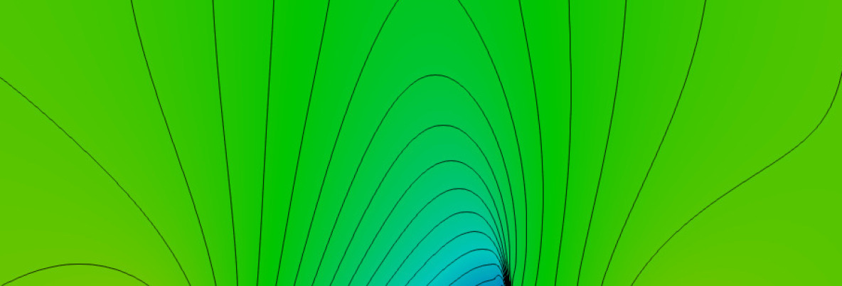
(a) Density

(b) Mach number

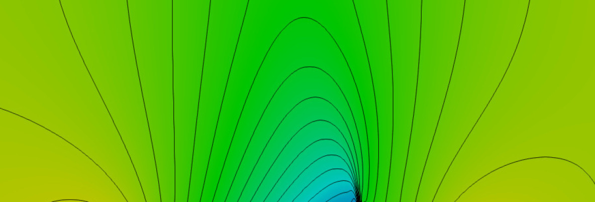
(c) Pressure

Figure 1: GAMM channel ($M_{\infty}=0.67$), steady-state MCL results obtained with $N_{h}=112,963$ unknowns per component on a mesh consisting of $E_{h}=224,576$ triangles.

Figure 2(b) shows the effect of changing the CFL number on the performance of the fixed-point iteration equipped with the adaptive underrelaxation strategy. We refer to the beginning of Section 6 for a general discussion of the way in which $\omega$ and CFL influence the convergence behavior.

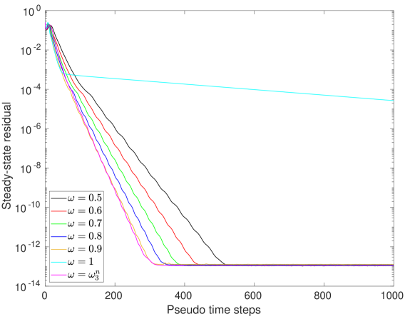
(a) Different underrelaxation factors, $\mathrm{CFL}=10^{4}$.

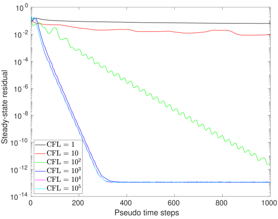
(b) Different CFL numbers, $\omega=\omega_{3}^{n}$.

Figure 2: GAMM channel ($M_{\infty}=0.67$), steady-state convergence history for a long-time MCL simulation on an unstructured triangular mesh with $N_{h}=24,037$ nodes and $E_{h}=47,256$ cells.

6.2 Converging-diverging nozzle

Next, we simulate steady gas flows in a two-dimensional converging-diverging nozzle [19, 22]. To evaluate the performance of our method under subsonic and transonic flow conditions, we consider three setups corresponding to different free stream Mach numbers. In all cases, we prescribe a subsonic inflow condition on the left boundary $\Gamma_{\mathrm{in}}=\{(x,y)\in\mathbb{R}^{2}:x=-2,\,-1\leq y\leq 1\}$. The upper and lower reflecting walls of the nozzle are defined by $\Gamma^{\pm}_{\mathrm{w}}=\{(x,g^{\pm}(x))\in\mathbb{R}^{2}:-2\leq x\leq 8\},$ where [22]

$$g^{\pm}(x)=\begin{cases}\pm 1&\text{if }-2\leq x\leq 0,\\ \pm\frac{\cos(\frac{\pi x}{2})+3}{4}&\text{if }0<x\leq 4,\\ \pm 1&\text{if }4<x\leq 8.\end{cases}$$

On the right boundary $\Gamma_{\mathrm{in}}=\{(x,y)\in\mathbb{R}^{2}:x=8,\,-1\leq y\leq 1\}$ of the domain, we prescribe a subsonic or supersonic outlet condition depending on the test case.

In the first setup [19], we define the free stream values on $\Gamma_{\mathrm{in}}$ using  (33) with $M_{\infty}=0.2$ and impose a subsonic outlet condition. The flow stays subsonic and accelerates to $M\approx 0.48$ at the throat before decelerating in the diverging part of the nozzle. The characteristic stiffness associated with low Mach numbers makes this problem very challenging despite the fact that the solution is smooth.

(a) Density

(b) Mach number

(c) Pressure

Figure 3: Subsonic nozzle ($M_{\infty}=0.2$), steady-state MCL results obtained with $N_{h}=95,329$ unknowns per component on a mesh consisting of $E_{h}=189,024$ triangles.

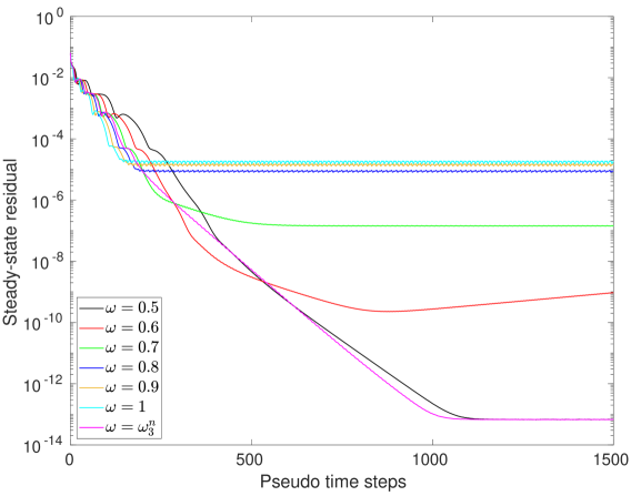
(d) Different underrelaxation factors, $\mathrm{CFL}=10^{4}$.

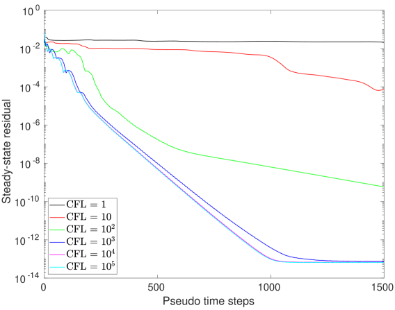
(e) Different CFL numbers, $\omega=\omega_{3}^{n}$.

Figure 4: Subsonic nozzle ($M_{\infty}=0.2$), steady-state convergence history for a long-time MCL simulation on an unstructured triangular mesh with $N_{h}=24,037$ nodes and $E_{h}=47,256$ cells.

(a) Density

(b) Mach number

(c) Pressure

Figure 5: Transonic nozzle ($M_{\infty}=0.3$), steady-state MCL results obtained with $N_{h}=95,329$ unknowns per component on a mesh consisting of $E_{h}=189,024$ triangles.

The steady-state MCL results and the convergence history for this test are shown in Fig. 4 and Fig. 4, respectively. In this low Mach number test, convergence to a stationary solution is achieved only with $\omega=0.5$ and with the adaptive strategy (31). In both cases, the stopping criterion $r(u)\leq 10^{-13}$ is met after $1000$ pseudo-time steps. All other choices of $\omega$ result in stagnation or even divergence (see Fig. 3(d)). Even for small CFL numbers, which introduce strong implicit underrelaxation, convergence is not guaranteed without additional explicit underrelaxation (not shown here). Similarly to the previous test case, the adaptive underrelaxation strategy exhibits the fastest convergence rate. The impact of the CFL number is illustrated by the evolution of steady-state residuals in Fig. 3(e). The convergence rates for $\mathrm{CFL}=10^{4}$ and $\mathrm{CFL}=10^{5}$ are similar and superior to that for $\mathrm{CFL}=10^{3}$.

The second setup induces a transonic flow. For better comparison with the literature [22], we prescribe the $M_{\infty}=0.3$ free stream values using the pressure $p_{\infty}=1$ instead of $p_{\infty}=1/\gamma$. The free stream velocity corresponding to $\rho_{\infty}=1$ is given by $\mathbf{v}_{\infty}=(\sqrt{\gamma}M_{\infty},0)^{\top}$. Furthermore, we prescribe $p_{\mathrm{out}}=\frac{2}{3}$ instead of the free stream pressure at the subsonic outlet. The resulting flow accelerates to $M\approx 2.1$ and develops a sonic shock, behind which it decelerates to subsonic speeds again.

As we observe in Fig. 6(a), solvers that use $\omega\in\{0.5,0.6,0.7,0.8,\omega^{n}_{3}\}$ do converge, while the residuals stagnate after a short initial phase for $\omega=1$ and $\omega=0.9$. The algorithm using the adaptive strategy (31) requires about 500 pseudo-time steps to meet the stopping criterion $r(u)\leq 10^{-13}$. As in the previous examples, convergence becomes faster as the CFL number is increased (see Fig. 6(b)).

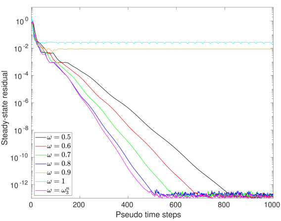
(a) Different underrelaxation factors, $\mathrm{CFL}=10^{4}$.

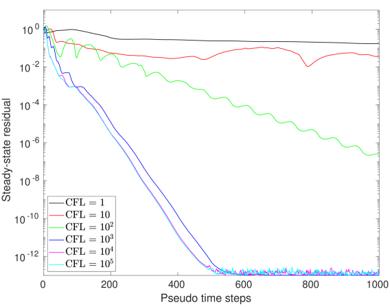
(b) Different CFL numbers, $\omega=\omega_{3}^{n}$.

Figure 6: Transonic nozzle ($M_{\infty}=0.3$), steady-state convergence history for a long-time MCL simulation on an unstructured triangular mesh with $N_{h}=24,037$ nodes and $E_{h}=47,256$ cells.

The last setup corresponds to a transonic flow with a supersonic outlet [19]. We define the free stream values using (33) with $M_{\infty}=0.8$. The flow is accelerated in the throat of the nozzle and stays supersonic. It features diamond-shaped shocks caused by reflections from the upper and lower walls. For this transonic flow setup, the steady-state computation fails to converge only if $\omega=1$ is employed. The adaptive strategy (31) meets the stopping criterion $r(u)\leq 10^{-13}$ after 300 pseudo-time steps. As we can see in Fig. 7, the use of $\omega=0.9$ gives rise to small fluctuations around the threshold $10^{-3}$. Figure 8(b) shows that $\mathrm{CFL}\geq 10^{3}$ is needed to achieve satisfactory convergence behavior.

(a) Density

(b) Mach number

(c) Pressure

Figure 7: Transonic nozzle ($M_{\infty}=0.8$), steady-state MCL results obtained with $N_{h}=95,329$ unknowns per component on a mesh consisting of $E_{h}=189,024$ triangles.

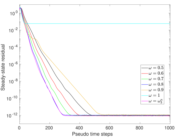
(a) Different underrelaxation factors, $\mathrm{CFL}=10^{4}$.

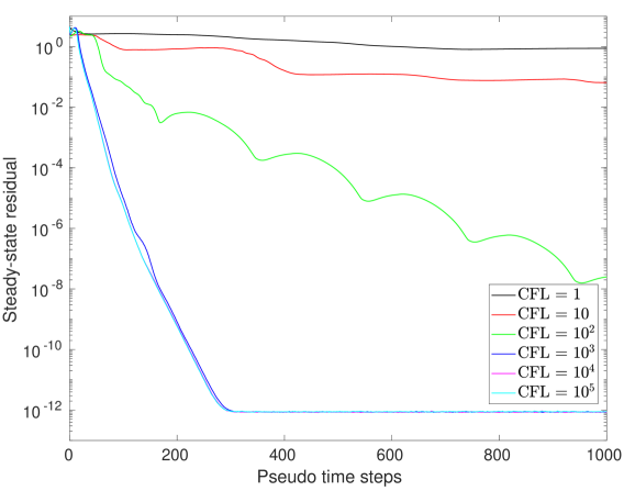
(b) Different CFL numbers, $\omega=\omega_{3}^{n}$.

Figure 8: Transonic nozzle ($M_{\infty}=0.8$), steady-state convergence history for a long-time MCL simulation on an unstructured triangular mesh with $N_{h}=24,037$ nodes and $E_{h}=47,256$ cells.

6.3 NACA 0012 airfoil

To further exemplify the typical convergence behavior of our scheme, we simulate external flows over a NACA 0012 airfoil. The upper and lower surface of this airfoil are defined by [19, 28]

$$\Gamma_{\pm}=\left\{(x,f_{\pm}(x))^{\top}\in\mathbb{R}^{2}:x\in[0,1.00893]\right\},$$

where

$$f_{\pm}(x)=\pm 0.6(0.2969\sqrt{x}-0.126x-0.3516x^{2}-0.1015x^{4}).$$

The outer boundary of the computational domain is a circle of radius 10 centered at the tip of the airfoil. The steady-state flow pattern depends on the Mach number and on the inclination angle.

In the first setup, we prescribe a $M_{\infty}=0.5$ free stream flow with the angle of attack $\alpha=0^{\circ}$. The steady state solutions and the convergence history are shown in Fig. 9 and Fig. 10, respectively. In the second series of experiments, we set $M_{\infty}=0.8$ and $\alpha=1.25^{\circ}$. The results are shown in Figs. 11 and 12. As expected, relaxation is needed to achieve convergence in the stiff subsonic test. Our adaptive relaxation strategy performs slightly better than the best manual choice of a constant relaxation factor ($\omega=0.9$). In the transonic test, convergence is achieved for all values of $\omega$. The best convergence rates are obtained with $\omega=1.0$ and $\omega=\omega_{3}^{n}$. For both choices of the Mach number $M_{\infty}$, steady-state computations with $\omega=\omega_{3}^{n}$ become faster as the value of the CFL number is increased.

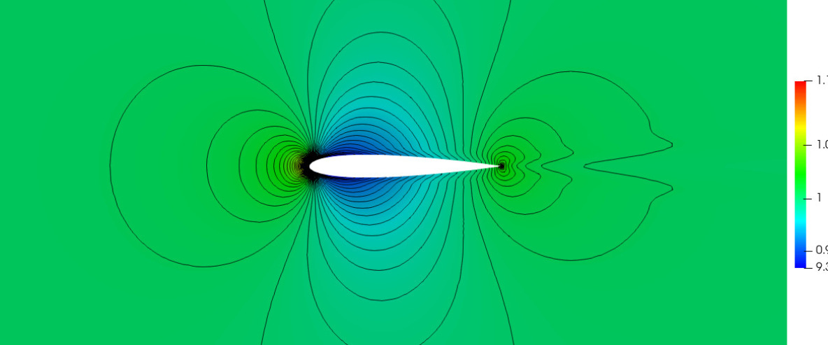
(a) Density

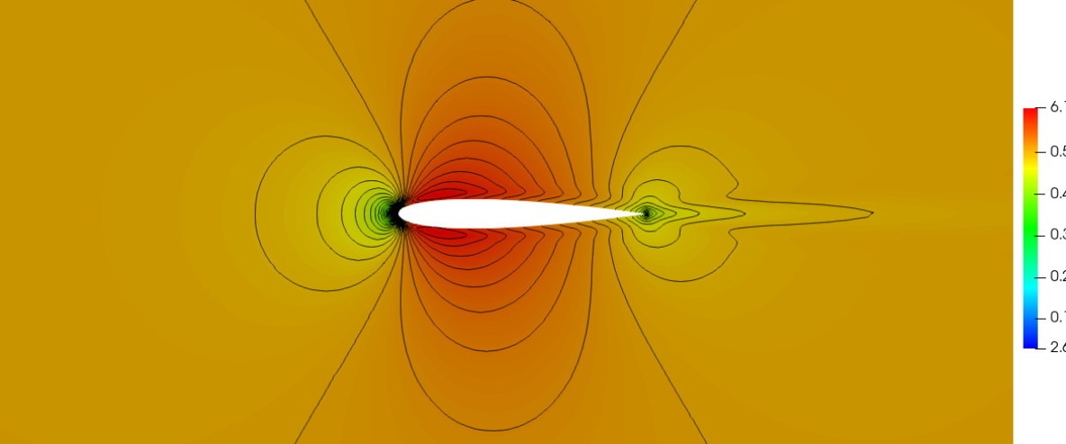
(b) Mach number

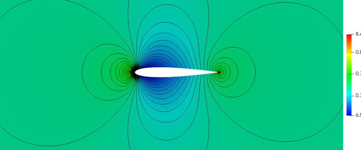
(c) Pressure

Figure 9: Subsonic NACA 0012 airfoil ($M_{\infty}=0.5$, $\alpha=0^{\circ}$), steady-state MCL results obtained with $N_{h}=112,242$ unknowns per component on a mesh consisting of $E_{h}=223,424$ triangles.

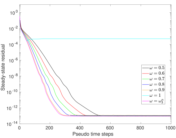
(a) Different underrelaxation factors, $\mathrm{CFL}=10^{4}$.

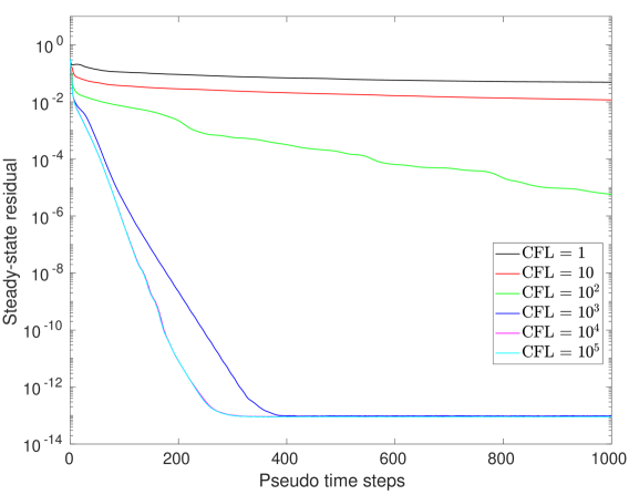
(b) Different CFL numbers, $\omega=\omega_{3}^{n}$.

Figure 10: Subsonic NACA 0012 airfoil ($M_{\infty}=0.5$, $\alpha=0^{\circ}$), steady-state convergence history for a long-time MCL simulation on an unstructured triangular mesh with $N_{h}=28,193$ nodes and $E_{h}=55,856$ cells.

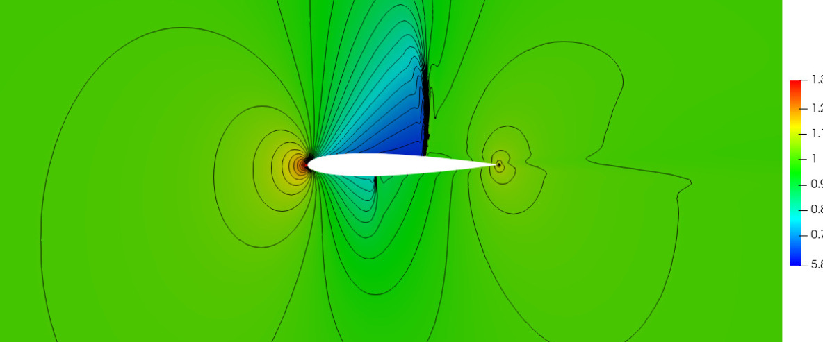
(a) Density

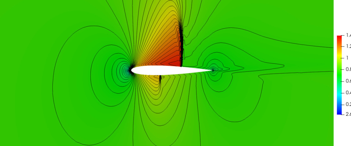
(b) Mach number

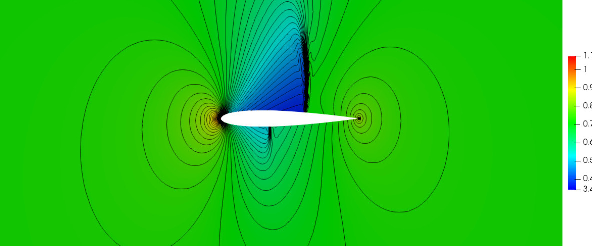
(c) Pressure

Figure 11: Transonic NACA 0012 airfoil at $\alpha=1.25^{\circ}$ angle ($M_{\infty}=0.8$), steady-state MCL results obtained with $N_{h}=112,242$ unknowns per component on a mesh consisting of $E_{h}=223,424$ triangles.

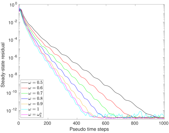
(a) Different underrelaxation factors, $\mathrm{CFL}=10^{4}$.

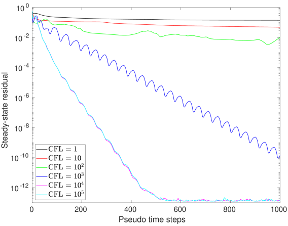
(b) Different CFL numbers, $\omega=\omega_{3}^{n}$.

Figure 12: Transonic NACA 0012 airfoil ($M_{\infty}=0.8$, $\alpha=1.25^{\circ}$), steady-state convergence history for a long-time MCL simulation on an unstructured triangular mesh with $N_{h}=28,193$ nodes and $E_{h}=55,856$ cells.

6.4 Mach 20 bow shock

We finish with an example in which we simulate a steady two-dimensional hypersonic flow around a half-cylinder of unit radius [8]. The free stream values at the supersonic inlet correspond to $M_{\infty}=20$. At the supersonic outlet, the external state of the weakly imposed boundary condition coincides with the internal limit. The abrupt transition from hypersonic to subsonic flow conditions at the bow of the cylinder makes this benchmark problem very challenging for linearized implicit solvers. To avoid divergence of nonlinear and linear iterations in the early stage of computations, we use pseudo-time steps corresponding to $\mathrm{CFL}=10$ until the relative residual falls below $10^{-1}$, that is, until

$$\|M_{L}^{-1}R_{\infty}^{*}(u^{n})\|_{2,h}<10^{-1}\|M_{L}^{-1}R_{\infty}^{*}(u^{0})\|_{2,h},$$

where $u^{0}$ is the low-order solution. We then switch to the target CFL number. The results presented in Figs. 13 and 14 illustrate the ability of our scheme to handle arbitrary Mach numbers.

(a) Density

(b) Mach number

(c) Pressure

Figure 13: Bow shock ($M_{\infty}=20$), steady-state MCL results obtained with $N_{h}=105,361$ unknowns per component on a mesh consisting of $E_{h}=209,152$ triangles.

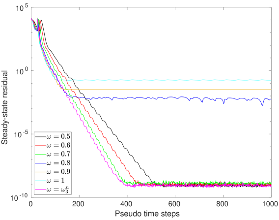
(a) Different underrelaxation factors, $\mathrm{CFL}=10^{4}$.

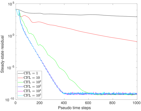
(b) Different CFL numbers, $\omega=\omega_{3}^{n}$.

Figure 14: Bow Shock ($M_{\infty}=20$), steady-state convergence history for a long-time MCL simulation on an unstructured triangular mesh with $N_{h}=26,537$ nodes and $E_{h}=52,288$ cells.

7 Conclusions

The analysis and algorithms presented in this paper illustrate the potential of monolithic convex limiting as an algebraic flux correction tool for implicit finite element discretizations of nonlinear hyperbolic systems. In addition to proving the existence of a positivity-preserving solution to the nonlinear discrete problem, we designed an iterative solver that exhibits robust convergence behavior and is well suited for steady-state computations. Two essential features of this solver are the stopping criterion based on positivity preservation and the use of relaxation parameters that minimize entropy residuals at steady state. The robustness of our method with respect to CFL and Mach numbers was verified numerically. Further improvements can presumably be achieved by using adaptive/local time stepping and local preconditioning aimed at reducing the characteristic condition number.

References

• [1] Rémi Abgrall. High order schemes for hyperbolic problems using globally continuous approximation and avoiding mass matrices. J. Sci. Comput., 73(2):461–494, 2017.
• [2] Robert Anderson, Julian Andrej, Andrew Barker, Jamie Bramwell, Jean-Sylvain Camier, Jakub Cerveny, Veselin Dobrev, Yohann Dudouit, Aaron Fisher, Tzanio Kolev, Will Pazner, Mark Stowell, Vladimir Tomov, Ido Akkerman, Johann Dahm, David Medina, and Stefano Zampini. MFEM: A modular finite element methods library. Comput. Math. Appl., 81:42–74, 2021.
• [3] Julian Andrej, Nabil Atallah, Jan-Phillip Bäcker, Jean-Sylvain Camier, Dylan Copeland, Veselin Dobrev, Yohann Dudouit, Tobias Duswald, Brendan Keith, Dohyun Kim, et al. High-performance finite elements with mfem. The International Journal of High Performance Computing Applications, page 10943420241261981, 2024.
• [4] Utkarsh Ayachit. The ParaView Guide: A Parallel Visualization Application. Kitware, 2015.
• [5] Santiago Badia and Jesús Bonilla. Monotonicity-preserving finite element schemes based on differentiable nonlinear stabilization. Computer Methods Appl. Meth. Engrg., 313:133–158, 2017.
• [6] Gabriel R Barrenechea, Volker John, and Petr Knobloch. Analysis of algebraic flux correction schemes. SIAM J. Numer. Anal., 54(4):2427–2451, 2016.
• [7] Abdallah Chalabi. On convergence of numerical schemes for hyperbolic conservation laws with stiff source terms. Mathematics of computation, 66(218):527–545, 1997.
• [8] Benoît Cossart, Jean-Philippe Braeunig, and Raphaël Loubère. Toward robust linear implicit schemes for steady state hypersonic flow. Preprint, available at SSRN: http://dx.doi.org/10.2139/ssrn.4820055, 2015.
• [9] Veselin Dobrev, Tzanio Kolev, Dmitri Kuzmin, Robert Rieben, and Vladimir Tomov. Sequential limiting in continuous and discontinuous Galerkin methods for the Euler equations. J. Comput. Phys., 356:372–390, 2018.
• [10] Vít Dolejší and Miloslav Feistauer. A semi-implicit discontinuous Galerkin finite element method for the numerical solution of inviscid compressible flow. Journal of Computational Physics, 198(2):727–746, 2004.
• [11] Vít Dolejší and Miloslav Feistauer. Discontinuous Galerkin Method. Analysis and Applications to Compressible Flow. Springer Series in Computational Mathematics, 48:234, 2015.
• [12] Miloslav Feistauer, Jiří Felcman, and Ivan Straškraba. Mathematical and Computational Methods for Compressible Flow. Oxford University Press, USA, 2003.
• [13] Joel H. Ferziger and Milovan Peric. Computational Methods for Fluid Dynamics. Springer, 3 edition, 2002.
• [14] C.A.J. Fletcher. The group finite element formulation. Computer Methods Appl. Meth. Engrg., 37(2):225–244, 1983.
• [15] Christophe Geuzaine and Jean-François Remacle. Gmsh: A 3-d finite element mesh generator with built-in pre-and post-processing facilities. Int. J. Numer. Methods Eng., 79(11):1309–1331, 2009.
• [16] Sigal Gottlieb, Chi-Wang Shu, and Eitan Tadmor. Strong stability-preserving high-order time discretization methods. SIAM Rev., 43(1):89–112, 2001.
• [17] Jean-Luc Guermond, Murtazo Nazarov, Bojan Popov, and Ignacio Tomas. Second-order invariant domain preserving approximation of the Euler equations using convex limiting. SIAM J. Sci. Comput., 40(5):A3211–A3239, 2018.
• [18] Jean-Luc Guermond and Bojan Popov. Invariant domains and first-order continuous finite element approximation for hyperbolic systems. SIAM J. Numer. Anal., 54(4):2466–2489, 2016.
• [19] Marcel Gurris. Implicit Finite Element Schemes for Compressible Gas and Particle-Laden Gas Flows. PhD thesis, TU Dortmund Univerity, 2009.
• [20] Marcel Gurris, Dmitri Kuzmin, and Stefan Turek. Implicit finite element schemes for the stationary compressible Euler equations. Int. J. Numer. Meth. Fluids, 69(1):1–28, 2012.
• [21] Hennes Hajduk. Algebraically Constrained Finite Element Methods for Hyperbolic Problems with Applications in Geophysics and Gas Dynamics. PhD thesis, TU Dortmund University, 2022.
• [22] Ralf Hartmann and Paul Houston. Adaptive discontinuous Galerkin finite element methods for the compressible Euler equations. Journal of Computational Physics, 183(2):508–532, 2002.
• [23] hypre: High performance preconditioners. https://llnl.gov/casc/hypre, https://github.com/hypre-space/hypre.
• [24] Dana A Knoll and David E Keyes. Jacobian-free Newton–Krylov methods: a survey of approaches and applications. Journal of Computational Physics, 193(2):357–397, 2004.
• [25] Václav Kučera, Mária Lukáčová-Medvid’ová, Sebastian Noelle, and Jochen Schütz. Asymptotic properties of a class of linearly implicit schemes for weakly compressible Euler equations. Numerische Mathematik, pages 1–25, 2022.
• [26] Dmitri Kuzmin. Monolithic convex limiting for continuous finite element discretizations of hyperbolic conservation laws. Computer Methods Appl. Meth. Engrg., 361:112804, 2020.
• [27] Dmitri Kuzmin and Hennes Hajduk. Property-Preserving Numerical Schemes for Conservation Laws. World Scientific, 2023.
• [28] Dmitri Kuzmin, Matthias Möller, and Marcel Gurris. Algebraic flux correction II. Compressible flow problems. In Dmitri Kuzmin, Rainald Löhner, and Stefan Turek, editors, Flux-Corrected Transport: Principles, Algorithms, and Applications, pages 193–238. Springer, 2 edition, 2012.
• [29] Dmitri Kuzmin, Matthias Möller, John N Shadid, and Mikhail Shashkov. Failsafe flux limiting and constrained data projections for equations of gas dynamics. J. Comput. Phys., 229(23):8766–8779, 2010.
• [30] Yimin Lin, Jesse Chan, and Ignacio Thomas. A positivity preserving strategy for entropy stable discontinuous Galerkin discretizations of the compressible Euler and Navier–Stokes equations. Journal of Computational Physics, 475:111850, 2023.
• [31] Christoph Lohmann. On the solvability and iterative solution of algebraic flux correction problems for convection-reaction equations. Preprint, Ergebnisber. Angew. Mathematik 612, TU Dortmund University, 2019.
• [32] Christoph Lohmann. Physics-Compatible Finite Element Methods for Scalar and Tensorial Advection Problems. Springer Spektrum, 2019.
• [33] Christoph Lohmann. An algebraic flux correction scheme facilitating the use of Newton-like solution strategies. Comput. Math. Appl., 84:56–76, 2021.
• [34] Christoph Lohmann and Dmitri Kuzmin. Synchronized flux limiting for gas dynamics variables. J. Comput. Phys., 326:973–990, 2016.
• [35] MFEM: Modular Finite Element Methods [Software]. https://mfem.org.
• [36] Suhas Patankar. Numerical Heat Transfer and Fluid Flow. CRC press, 1980.
• [37] Rolf Rannacher. Einführung in die Numerische Mathematik. Deutsche Nationalbibliothek, 2017.
• [38] Hendrik Ranocha, Mohammed Sayyari, Lisandro D. Dalcin, Matteo Parsani, and David I. Ketcheson. Relaxation Runge–Kutta methods: Fully discrete explicit entropy-stable schemes for the compressible Euler and Navier–Stokes equations. SIAM J. Sci. Comput., 42(2):A612–A638, 2020.
• [39] Philip L Roe. Approximate Riemann solvers, parameter vectors, and difference schemes. J. Comput. Phys., 43(2):357–372, 1981.
• [40] Andrés M. Rueda-Ramírez, Benjamin Bolm, Dmitri Kuzmin, and Gregor J. Gassner. Monolithic convex limiting for Legendre-Gauss-Lobatto discontinuous Galerkin spectral-element methods. Commun. Appl. Math. & Computation, pages 1–39, 2024.
• [41] Hua-Zhong Tang and Kun Xu. Positivity-preserving analysis of explicit and implicit Lax–Friedrichs schemes for compressible Euler equations. J. Sci. Computing, 15:19–28, 2000.
• [42] Stefan Turek. Efficient Solvers for Incompressible Flow Problems: An Algorithmic and Computational Approach. Springer, 1999.