HERA: High-efficiency Matrix Compression via Element Replacement

Abstract

Large Language Models (LLMs) have significantly advanced natural language processing tasks such as machine translation, text generation, and sentiment analysis. However, their large size, often consisting of billions of parameters, poses challenges for storage, computation, and deployment, particularly in resource-constrained environments like mobile devices and edge computing platforms. Additionally, the key-value (k-v) cache used to speed up query processing requires substantial memory and storage, exacerbating these challenges. Vector databases have emerged as a crucial technology to efficiently manage and retrieve the high-dimensional vectors produced by LLMs, facilitating faster data access and reducing computational demands.

Effective compression and quantization techniques are essential to address these challenges, as they reduce the memory footprint and computational requirements without significantly compromising performance. Traditional methods that uniformly map parameters to compressed spaces often fail to account for the uneven distribution of parameters, leading to considerable accuracy loss. Therefore, innovative approaches are needed to achieve better compression ratios while preserving model performance.

In this work, we propose HERA, a novel algorithm that employs heuristic Element Replacement for compressing matrix. HERA systematically replaces elements within the model using heuristic methods, which simplifies the structure of the model and makes subsequent compression more effective. By hierarchically segmenting, compressing, and reorganizing the matrix dataset, our method can effectively reduce the quantization error to 12.3% of the original at the same compression ratio.

1 Introduction

Large Language Models (LLMs) have revolutionized the field of natural language processing (NLP), enabling significant advancements in tasks such as machine translation, text generation, and sentiment analysis. These models, characterized by their large-scale neural network architectures and vast training datasets, have shown remarkable capabilities in understanding and generating human language. The advent of LLMs, such as OpenAI’s GPT-3 and BERT by Google, has pushed the boundaries of what machines can achieve in linguistic tasks, providing near-human performance in various applications  Brown et al. (2020); Devlin et al. (2018).

The development of LLMs is rooted in the transformer architecture, which employs self-attention mechanisms to process and produce language with high contextual relevance. This architecture has replaced previous recurrent neural network (RNN) and long short-term memory (LSTM) models due to its efficiency and ability to handle long-range dependencies in text Vaswani et al. (2017). As a result, LLMs have become the cornerstone of modern NLP, driving innovations in areas such as automated customer service, content creation, and real-time language translation.

Furthermore, the development and deployment of LLMs face significant challenges, particularly in optimizing vector database efficiency, LLM weight quantization, and key-value (k-v) cache optimization. First, as the size and complexity of LLMs increase, efficiently managing and retrieving vectors in large databases becomes critical. Optimizing vector database efficiency involves improving indexing and search algorithms to handle high-dimensional data, which is essential for tasks like semantic search and recommendation systems Johnson et al. (2019). Second, LLM weight quantization, which involves reducing the precision of model weights, is a crucial technique for making these models more storage and computation efficient without significantly degrading their performance. Quantization can drastically reduce the memory footprint and computational requirements, enabling the deployment of LLMs on resource-constrained devices. However, achieving optimal quantization while maintaining model accuracy remains a complex challenge that requires sophisticated algorithms and techniques Dettmers et al. (2021). Lastly, optimizing k-v cache efficiency is vital for speeding up inference times in LLMs. The k-v cache stores intermediate activations during the forward pass, which can be reused to avoid redundant computations. Efficient management and compression of these caches are essential to reduce latency and improve the throughput of LLMs, especially in real-time applications like chatbots and virtual assistants.

Figure 1: The distribution of LLM parameter.

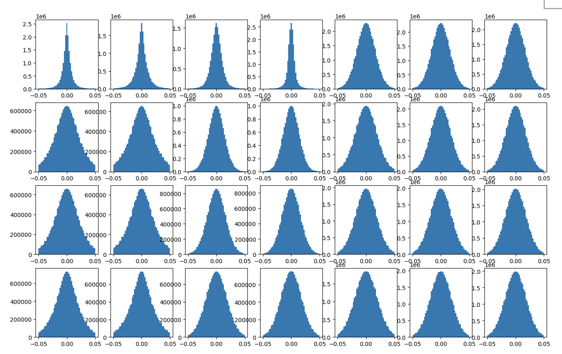
To address the challenges of storage and computational efficiency in large language models (LLMs), it is crucial to develop techniques that optimize vector database efficiency, weight quantization, and key-value (k-v) cache optimization. Therefore, finding quantization algorithms that can efficiently compress and quickly decompress matrix data is essential.

In practice, when compressing parameters, the distribution of parameters is often uneven. First, the distribution is not uniform, and second, the magnitudes of different data points vary significantly. For example, the distribution of Transformer neural network weights is shown in Figure  1. In Figure  1, different rows represent the 0th layer, 8th layer, 16th layer, and 24th layer. Different columns represent the attention layer’s q, k, v, and o layers, as well as the fully connected layer’s gate, up, and down layers. The distributions of different layers are not uniformly analyzed, and the distributions vary across different layers. Previous algorithms uniformly and linearly map parameters to another compressed space. Although this method is simple, it may not be effective and can result in significant accuracy loss because it does not take into account the original data distribution. It maps both densely populated and sparse regions to the quantized space in the same way. Besides, A lines of works have been proposed to optimize vector database efficiency Ge et al. (2013); Jegou et al. (2010); Kalantidis, Avrithis (2014), quantize the model weights Dettmers et al. (2022); Polino et al. (2018); Chmiel et al. (2020); Fan et al. (2020); Zafrir et al. (2019); Wu et al. (2022); LeCun et al. (1989) and optimizate kv cache Hooper et al. (2024); Cho et al. (2024). They also does not take into account the original data distribution. Therefore, a more reasonable approach is to quantize the model based on the distribution and magnitude of the parameters, stratifying and computing accordingly.

In this work, we propose a novel algorithm named HERA to enhance the compression of large language models. The core idea of HERA is to group the relevant matrices and compress each group using clustering methods. Furthermore, HERA reorders the original dataset based on the distribution and magnitude of the parameters. This reordering is performed in multiple layers, with each layer featuring a new arrangement that optimizes the dataset’s distribution for compression. By leveraging these techniques, HERA effectively reduces data error and minimizes the discrepancy between estimated data and actual data.

We implemented a prototype system using Python. Experimental results show that, by hierarchically segmenting, compressing, and reorganizing the matrix dataset, our method can effectively reduce the quantization error to 12.3% of the original at the same compression ratio.

2 HERA

2.1 Basic algorithm

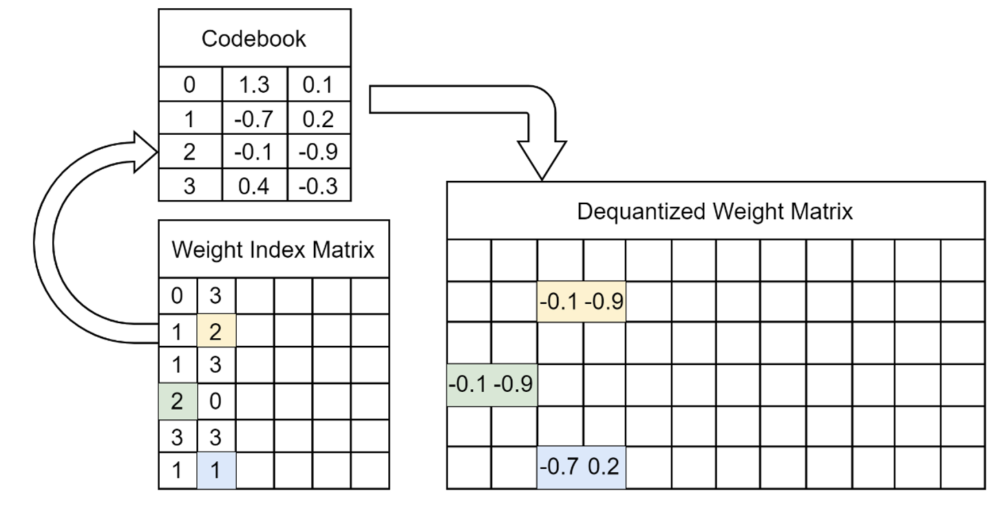
We borrow the idea from product quantization algorithm and k-means algorithm to compress the model parameter. The algorithm is divided into four steps, the first three steps is quantization process as shown in Figure  2, the last two steps is the dequantization process as show in Figure  3. The detailed process is described below.

Algorithm 1 Product Quantization Algorithm

1:$X\in\mathbb{R}^{N\times D}$ $\triangleright$ Input matrix

2:Quantization Process:

3:Step 1: Space Partitioning

4:for each vector $x_{i}$ in $X$ do

5:     Divide $x_{i}$ into $M$ low-dimensional subspaces $x_{i}^{1},x_{i}^{2},\ldots,x_{i}^{M}$

6:end for

7:Step 2: Codebook Calculation

8:for each subspace $j$ from 1 to $M$ do

9:     Apply k-means algorithm to subspace $j$ to get $k$ cluster centers

10:     Create codebook $C_{j}$ for subspace $j$ with cluster centers

11:end for

12:Step 3: Quantization

13:for each vector $x_{i}$ in $X$ do

14:     for each subspace $j$ from 1 to $M$ do

15:         Map $x_{i}^{j}$ to the nearest cluster center in $C_{j}$

16:     end for

17:end for

18:Dequantization Process:

19:Step 4: Codebook Reconstruction

20:Construct a global codebook $C$ that contains all possible combinations of cluster centers from $C_{1},C_{2},\ldots,C_{M}$

21:Step 5: Dequantization

22:for each quantized vector $q_{i}$ in the quantized dataset do

23:     Restore $q_{i}$ to its original high-dimensional space using the global codebook $C$

24:end for

1. Space Partitioning: Divide the high-dimensional space into a series of low-dimensional subspaces.

2. Codebook calculation: Use k-means algorithm to calculate codebook of low-dimensional subspaces.

3. Quantization: Perform independent quantization within each low-dimensional subspace, mapping data points to the nearest cluster center.

4. Codebook Reconstruction: Reconstruct the data using a codebook that contains all possible cluster centers.

5. Dequantization: Restore the vectors in the original high-dimensional space based on the vectors in the quantized low-dimensional subspaces.

Figure 2: The Quantization Process of HERA.

Figure 3: The Dequantization Process of HERA.

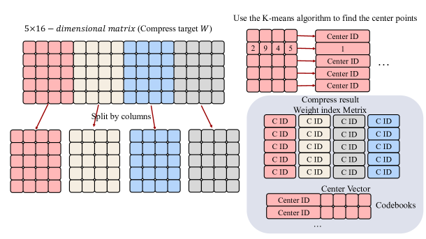
In data matrices where the distribution of data is uneven across different columns, directly applying the k-means algorithm for clustering may yield suboptimal results. This unevenness can distort the clustering process, as k-means assumes that all features contribute equally to the distance calculations. The differing distributions across columns mean that some features may disproportionately influence the clustering outcome, leading to biased clusters that do not accurately reflect the true structure of the data.

To mitigate these effects, it is crucial to preprocess the data appropriately. One common approach is to normalize the data so that each column contributes equally to the distance metric used by k-means. Standard normalization techniques, such as z-score normalization or min-max scaling, can be employed to transform the data into a more uniform distribution. By ensuring that all features are on a comparable scale, the k-means algorithm can perform more effectively, producing clusters that better represent the underlying patterns in the data.

Algorithm 2 Product Quantization with HERA heuristics

1:Input matrix: $X\in\mathbb{R}^{N\times D}$, number of iteration in HERA: $iter$.

2:Quantized feature matrix and feature map

3:for each element $x_{i}\in X$ do

4:     Rearrange $X$ into pairs: $X_{\text{pairs}}\in\mathbb{R}^{N\times D/2}$

5:     for each dimension $j$ do

6:         $x_{pair_{i,j}}=(x_{2i,j},x_{2i+1,j})\in X_{\text{pairs}}$

7:     end for

8:end for

9:for each pair $x_{pair_{i,j}}$ in $X_{\text{pairs}}$ do

10:     if $x_{pair_{i,j}}[1]<x_{pair_{i,j}}[2]$ then

11:         $X[iter]_{small_{i,j}}\leftarrow x_{pair_{i,j}}[1]$

12:         $X[iter]_{big_{i,j}}\leftarrow x_{pair_{i,j}}[2]$

13:         $fm[iter]_{i,j}\leftarrow 1$

14:     else

15:         $X[iter]_{small_{i,j}}\leftarrow x_{pair_{i,j}}[2]$

16:         $X[iter]_{big_{i,j}}\leftarrow x_{pair_{i,j}}[1]$

17:         $fm[iter]_{i,j}\leftarrow 0$

18:     end if

19:end for

20:for $X_{small}$ and $X_{large}$ do

21:     code[$iter$], codebook [$iter$] $\leftarrow$ PQ($X[iter]_{small}$)

22:     code[$iter$], codebook[$iter$] $\leftarrow$ PQ($X[iter]_{large}$)

23:end for

24:$iter$ $\leftarrow$ $iter$ - 1

25:if $iter$ $\neq$ 0 then

26:     Goto line 1

27:end if

However, these transformations require specific parameters for each column and involve complex calculations, which can be computationally intensive and demand significant storage resources. To address this, we employ a reordering method that permutations the elements of the matrix based on their relative sizes. This approach achieves a more uniform distribution, enabling more effective application of compression operations.

Algorithm 3 Dequantization of Product Quantization with HERA heuristics

1:Quantized feature matrices: $code_{small}$, $code_{big}$, codebooks: $codebook_{small}$, $codebook_{big}$, feature maps: $fm$, number of iterations in HERA: $iter$

2:Reconstructed matrix: $\hat{X}\in\mathbb{R}^{N\times D}$

3:Initialize $\hat{X}_{pairs}\in\mathbb{R}^{N\times D/2}$

4:for each iteration from $1$ to $iter$ do

5:     for each pair $x_{pair_{i,j}}$ in $\hat{X}_{pairs}$ do

6:         $\hat{X}_{small_{i,j}}\leftarrow\text{decode}(code_{small}[iter],codebook_{small}[iter])$

7:         $\hat{X}_{big_{i,j}}\leftarrow\text{decode}(code_{big}[iter],codebook_{big}[iter])$

8:     end for

9:     for each pair $x_{pair_{i,j}}$ in $\hat{X}_{pairs}$ do

10:         if $fm[iter]_{i,j}=1$ then

11:              $x_{pair_{i,j}}[1]\leftarrow\hat{X}_{small_{i,j}}$

12:              $x_{pair_{i,j}}[2]\leftarrow\hat{X}_{big_{i,j}}$

13:         else

14:              $x_{pair_{i,j}}[2]\leftarrow\hat{X}_{small_{i,j}}$

15:              $x_{pair_{i,j}}[1]\leftarrow\hat{X}_{big_{i,j}}$

16:         end if

17:     end for

18:end for

19:for each dimension $j$ do

20:     for each element $i$ in $\hat{X}_{pairs}$ do

21:         $\hat{x}_{2i,j}\leftarrow x_{pair_{i,j}}[1]$

22:         $\hat{x}_{2i+1,j}\leftarrow x_{pair_{i,j}}[2]$

23:     end for

24:end for

The purpose of permutation is to explore all possible reordering methods within the search space. For an $N\times D$ matrix, there are $(N!)^{D}$ possible permutations, creating a vast search space.

To manage this, we employ heuristic algorithms to reduce the search space and optimize the algorithm’s complexity. Heuristic algorithms provide approximate solutions by focusing on the most promising areas of the search space, rather than exhaustively evaluating all possible permutations. These methods significantly decrease computational requirements while still delivering high-quality solutions.

By adopting this heuristic reordering strategy, we aim to achieve a more balanced distribution of data across the matrix. This not only simplifies the preprocessing steps but also enhances the efficiency of subsequent clustering and compression processes. Ultimately, this method helps overcome the challenges posed by uneven data distributions, leading to more accurate and resource-efficient clustering outcomes.

2.2 HERA heuristics

To improve quantization and avoid uneven distribution, HERA first perceives the distribution of data sizes, then rearranges the elements according to the distribution, and finally quantizes the rearranged matrix.

2.2.1 HERA Design

We observe that compressing matrix elements of similar sizes as a single column (group) yields better results.HERA uses a low-cost method to locally adjust element arrangement based on data sizes. We first introude the HERA design. The design of HERA heuristics is shown in Figure  4.

Figure 4: HERA heuristics.

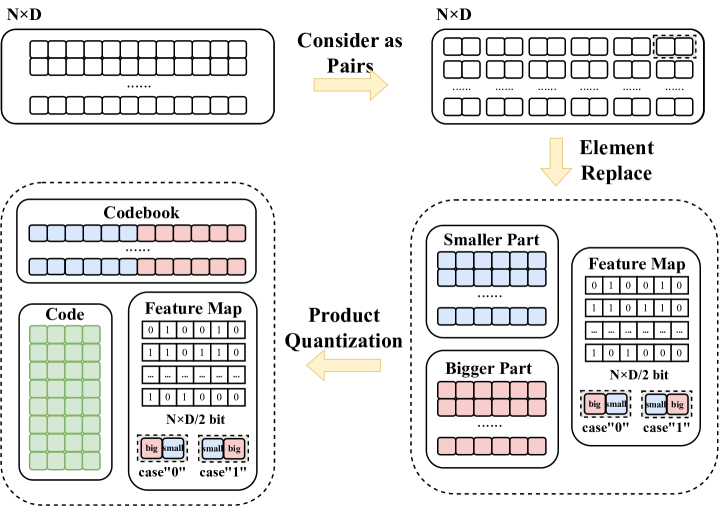
HERA groups every two elements in the matrix together, rearranges the matrix elements based on the size of adjacent elements, and then quantizes the rearranged results.

Quantization: The quantization process is illustrated in the algorithm 2, the quantization process consists of multiple steps, which involve rearranging the input data, comparing elements, and quantizing both smaller and larger value sets.

The algorithm begins by rearranging the input matrix $X\in\mathbb{R}^{N\times D}$ into pairs (lines 1 in Algorithm 2). Each element $x_{i}\in X$ is grouped into $X_{\text{pairs}}\in\mathbb{R}^{N\times D/2}$ by combining every two consecutive elements along each dimension. For each dimension $j$, the pairs are formed as $(x_{2i,j},x_{2i+1,j})$ (lines 2–4 in Algorithm 2).

Next, each pair $x_{pair_{i,j}}$ is compared to separate the smaller and larger values. If the first element of the pair is smaller, it is assigned to $X_{small}$ and the second to $X_{big}$, with a feature map $fm$ recording the comparison result as 1 (lines 5–8 in Algorithm 2). Otherwise, the assignment is reversed, and the feature map records a 0 (lines 9–12 in Algorithm 2).

The quantization process proceeds by applying the PQ algorithm to both $X_{small}$ and $X_{big}$. This process is iteratively repeated for a predefined number of iterations ($iter$), refining the quantization results with each iteration (lines 13–16 in Algorithm 2).

Dequantization:The Decompression process consists of multiple steps, namely decoding the quantized values, reconstructing the pairs, and restoring the original matrix dimensions.

The algorithm begins by initializing the reconstructed matrix $\hat{X}_{pairs}\in\mathbb{R}^{N\times D/2}$ (line 1 in Algorithm 3). For each iteration, the algorithm decodes the quantized values from the codebooks for both small and large pairs (lines 2–4 in Algorithm 3). The decoded values are stored in $\hat{X}_{small}$ and $\hat{X}_{big}$ respectively.

Next, for each pair in $\hat{X}_{pairs}$, the algorithm reconstructs the pairs based on the feature map $fm[iter]$. If the feature map value is 1, the first element of the pair is assigned the decoded small value and the second element the decoded big value (lines 5–8 in Algorithm 3). If the feature map value is 0, the assignment is reversed (lines 9–12 in Algorithm 3).

Finally, the pairs are expanded back into the original dimensions to form the reconstructed matrix $\hat{X}$ (lines 13–17 in Algorithm 3).

3 Experiments

3.1 Experiment setup

Dataset: The datasets used in our experiments were generated with matrices of size $N\times D$, where $N$ is the number of samples and $D$ is the dimensionality of each sample. We employed one types of normal distribution to create these datasets.

Normal Distribution Dataset: For the normal distribution dataset, each element of the matrix was drawn from a truncated normal distribution with a mean of 0.5 and a standard deviation of 0.16. The distribution was truncated to the open interval $(0,1)$ to ensure all values remain within this range.

$$\mathbf{X}_{ij}\sim\mathcal{TN}(0.5,0.16,0,1),\quad\forall i\in\{1,\ldots,N\},\quad\forall j\in\{1,\ldots,D\}$$

Here, $\mathcal{TN}(\mu,\sigma,a,b)$ denotes the truncated normal distribution with mean $\mu$, standard deviation $\sigma$, truncated to the interval $(a,b)$.

Platform and implementation: We conducted our algorithm evaluations on a high-performance server equipped with an Intel Core i9-10980XE processor, featuring 18 cores and 36 threads, operating at a base frequency of 3.00 GHz. The server also includes 128GB of 3200MHz DDR4 memory and a 24.8MB L3 cache, providing robust computational capabilities. All algorithms were implemented in Python, using version 3.8.10. For each case, the experiment was repeated 100 times. In each repetition, matrices of the same size and from the same distribution were generated using different seeds.

Comparison of Algorithms and Parameter Selection

In this section, we describe the parameter selection process for our HERA algorithm and compare its performance with the Optimized Product Quantization (OPQ) algorithm.

Our HERA algorithm involves a critical parameter, the number of centroids $K_{s}$. The selection of $K_{s}$ is governed by the following memory constraint:

$$K_{s}\times D\times 32+N\times M\times[(K_{s}-1)\cdot\text{bitlength}]\leq\text{memory in bits}$$

where:

• $K_{s}$ is the number of centroids,

• $D$ is the dimensionality of each sample,

• $N$ is the number of samples,

• $M$ is the number of subspaces,

• bitlength is the bit length used for encoding.

This constraint ensures that the total memory usage remains within the available memory limits. By carefully selecting $K_{s}$, we aim to optimize the performance of the HERA algorithm while adhering to memory constraints.

The Optimized Product Quantization (OPQ) algorithm was used as a benchmark for comparison. The OPQ algorithm was implemented with default parameters, providing a consistent basis for performance evaluation. The OPQ algorithm optimizes product quantization by adjusting the space partitioning and centroid assignments to minimize quantization error.

Comparison Metrics

We use MAE (Mean Absolute Error), MRE (Mean Relative Error), and MSE (Mean Squared Error) for experimental evaluation. Let $X_{(i,j)}$ and $X_{(i,j)}^{\prime}$ denote the values before and after dequantization, respectively. The following metrics are used for comparison:

$$\text{MAE}=\frac{1}{N\cdot D}\sum_{i,j}\left|X_{(i,j)}-X_{(i,j)}^{\prime}\right|$$

$$\text{MRE}=\frac{1}{N\cdot D}\sum_{i,j}\frac{\left|X_{(i,j)}-X_{(i,j)}^{\prime}\right|}{X_{(i,j)}}$$

$$\text{MSE}=\frac{1}{N\cdot D}\sum_{i,j}\left(X_{(i,j)}-X_{(i,j)}^{\prime}\right)^{2}$$

We performed an optimization using 1-4 iterations, corresponding to our algorithms labeled as our1 through our4. In the quantification accuracy experiment, we tested the accuracy with different numbers of groups $m$ and various sizes of data matrices. In the sensitivity experiment, we evaluated the impact of different numbers of groups $m$ on the results while maintaining the same compression ratio.

3.2 Experiment result

Accuracy Measurement

Figure 5: MAE on 8 subspaces.

Figure 6: MRE on 8 subspaces.

Figure 7: MSE on 8 subspaces.

Figure 8: MAE on 16 subspaces.

Figure 9: MRE on 16 subspaces.

Figure 10: MSE on 16 subspaces.

Figure 11: MAE on 32 subspaces.

Figure 12: MRE on 32 subspaces.

Figure 13: MSE on 32 subspaces.

Figure 14: MAE on 128 subspaces.

Figure 15: MRE on 128 subspaces.

Figure 16: MSE on 128 subspaces.

Figure 17: MAE on 1 iterations.

Figure 18: MRE on 1 iterations.

Figure 19: MSE on 1 iterations.

Figure 20: MAE on 2 iterations.

Figure 21: MRE on 2 iterations.

Figure 22: MSE on 2 iterations.

Figure 23: MAE on 3 iterations.

Figure 24: MRE on 3 iterations.

Figure 25: MSE on 3 iterations.

Figure 26: MAE on 4 iterations.

Figure 27: MRE on 4 iterations.

Figure 28: MSE on 4 iterations.

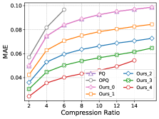
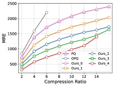
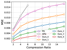
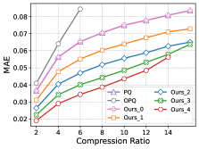
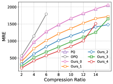
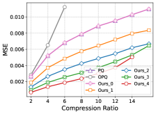
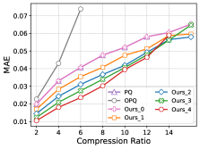
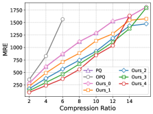
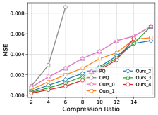
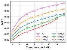
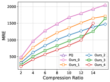
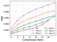
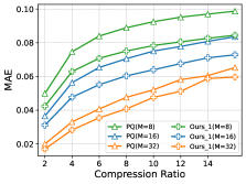
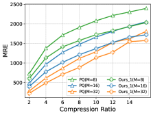
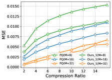
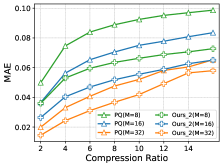
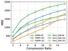
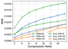
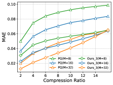
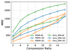
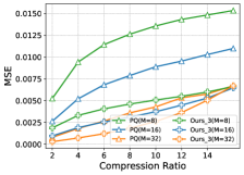
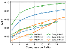
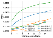
We measure MAE, MRE and MSE on different numbers of subspaces to show the accuracy of HERA.The results for MAE, MRE and MSE for different number of subspaces are shown in Figures  7-  7, Figures  10-  10, Figures  13-  13, Figures  16-  16 respectively. For 8-subspace setting, HERA can reduce the MSE to 70.4%, 49.7%, 35.1% and 12.3% in 1-4 iterations, respectively.

From the experimental results, we can derive four conclusions. Firstly, the higher the compression ratio, the less space is consumed, but the accuracy decreases. Secondly, the OPQ algorithm performs worse than others with the same compression rate because it needs to store the transformation matrix. Additionally, the PQ algorithm does not perform as well as our improved algorithm. Finally, the more iterations, the better the performance of our algorithm.

Parameter sensitivity analysis: We also conducted a parameter sensitivity test under different iterations, evaluating how the number of subspaces affects the algorithm’s performance. The results for 1 to 4 iterations are shown in Figures  19- 19, Figures  22- 22, and Figures  25- 25, respectively. Extensive experiments demonstrate that our algorithm reduces parameter sensitivity, making parameter selection more user-friendly (as indicated by the closer proximity of parameters in our algorithm’s curves).

4 Conclusion

In conclusion, our research addresses critical challenges in the optimization of large language models (LLMs) through the development of a novel algorithm, HERA. The growing complexity and scale of LLMs necessitate innovative approaches to enhance storage and computational efficiency, particularly in vector database management, weight quantization, and key-value (k-v) cache optimization.

HERA’s hierarchical approach to segmenting, compressing, and reorganizing the matrix dataset has proven to be effective in significantly reducing quantization error. By considering the distribution and magnitude of parameters, our method achieves superior performance compared to traditional uniform quantization techniques. The experimental results from our prototype system, implemented in Python, demonstrate that HERA can reduce the quantization error to 12.3% of the original, maintaining the same compression ratio.

Future work will explore further refinements to HERA, including its application to other types of application and broader datasets. Additionally, investigating the integration of HERA with other optimization techniques may yield even greater enhancements in model performance and efficiency. The promising results of this study encourage continued research and development in the quest for more effective and scalable solutions for LLM compression and optimization.

References

- Brown et al. (2020) Brown Tom, Mann Benjamin, Ryder Nick, Subbiah Melanie, Kaplan Jared D, Dhariwal Prafulla, Neelakantan Arvind, Shyam Pranav, Sastry Girish, Askell Amanda, others . Language models are few-shot learners // Advances in neural information processing systems. 2020. 33. 1877–1901.
- Chmiel et al. (2020) Chmiel Brian, Banner Ron, Shomron Gil, Nahshan Yury, Bronstein Alex, Weiser Uri, others . Robust quantization: One model to rule them all // Advances in neural information processing systems. 2020. 33. 5308–5317.
- Cho et al. (2024) Cho Minsik, Rastegari Mohammad, Naik Devang. KV-Runahead: Scalable Causal LLM Inference by Parallel Key-Value Cache Generation // arXiv preprint arXiv:2405.05329. 2024.
- Dettmers et al. (2022) Dettmers Tim, Lewis Mike, Belkada Younes, Zettlemoyer Luke. Llm. int8 (): 8-bit matrix multiplication for transformers at scale // CoRR abs/2208.07339. 2022.
- Dettmers et al. (2021) Dettmers Tim, Lewis Mike, Shleifer Sam, Zettlemoyer Luke. 8-bit optimizers via block-wise quantization // arXiv preprint arXiv:2110.02861. 2021.
- Devlin et al. (2018) Devlin Jacob, Chang Ming-Wei, Lee Kenton, Toutanova Kristina. Bert: Pre-training of deep bidirectional transformers for language understanding // arXiv preprint arXiv:1810.04805. 2018.
- Fan et al. (2020) Fan Angela, Stock Pierre, Graham Benjamin, Grave Edouard, Gribonval Rémi, Jegou Herve, Joulin Armand. Training with quantization noise for extreme model compression // arXiv preprint arXiv:2004.07320. 2020.
- Ge et al. (2013) Ge Tiezheng, He Kaiming, Ke Qifa, Sun Jian. Optimized product quantization // IEEE transactions on pattern analysis and machine intelligence. 2013. 36, 4. 744–755.
- Hooper et al. (2024) Hooper Coleman, Kim Sehoon, Mohammadzadeh Hiva, Mahoney Michael W, Shao Yakun Sophia, Keutzer Kurt, Gholami Amir. Kvquant: Towards 10 million context length llm inference with kv cache quantization // arXiv preprint arXiv:2401.18079. 2024.
- Jegou et al. (2010) Jegou Herve, Douze Matthijs, Schmid Cordelia. Product quantization for nearest neighbor search // IEEE transactions on pattern analysis and machine intelligence. 2010. 33, 1. 117–128.
- Johnson et al. (2019) Johnson Jeff, Douze Matthijs, Jégou Hervé. Billion-scale similarity search with GPUs // IEEE Transactions on Big Data. 2019. 7, 3. 535–547.
- Kalantidis, Avrithis (2014) Kalantidis Yannis, Avrithis Yannis. Locally optimized product quantization for approximate nearest neighbor search // Proceedings of the IEEE conference on computer vision and pattern recognition. 2014. 2321–2328.
- LeCun et al. (1989) LeCun Yann, Denker John, Solla Sara. Optimal brain damage // Advances in neural information processing systems. 1989. 2.
- Polino et al. (2018) Polino Antonio, Pascanu Razvan, Alistarh Dan. Model compression via distillation and quantization // arXiv preprint arXiv:1802.05668. 2018.
- Vaswani et al. (2017) Vaswani Ashish, Shazeer Noam, Parmar Niki, Uszkoreit Jakob, Jones Llion, Gomez Aidan N, Kaiser Łukasz, Polosukhin Illia. Attention is all you need // Advances in neural information processing systems. 2017. 30.
- Wu et al. (2022) Wu Xiaoxia, Yao Zhewei, Zhang Minjia, Li Conglong, He Yuxiong. Xtc: Extreme compression for pre-trained transformers made simple and efficient // Advances in Neural Information Processing Systems. 2022. 35. 3217–3231.
- Zafrir et al. (2019) Zafrir Ofir, Boudoukh Guy, Izsak Peter, Wasserblat Moshe. Q8bert: Quantized 8bit bert // 2019 Fifth Workshop on Energy Efficient Machine Learning and Cognitive Computing-NeurIPS Edition (EMC2-NIPS). 2019. 36–39.