Orthogonal Constrained Minimization with Tensor $\ell_{2,{p}}$ Regularization for HSI Denoising and Destriping

Abstract

Hyperspectral images (HSIs) are often contaminated by a mixture of noises such as Gaussian noise, dead lines, stripes, and so on. In this paper, we propose a novel approach for HSI denoising and destriping, called NLTL2p, which consists of an orthogonal constrained minimization model and an iterative algorithm with convergence guarantees. The model of the proposed NLTL2p approach is built based on a new sparsity-enhanced Nonlocal Low-rank Tensor regularization and a tensor $\ell_{2,p}$ norm with $p\in(0,1)$. The low-rank constraints for HSI denoising utilize the spatial nonlocal self-similarity and spectral correlation of HSIs and are formulated based on independent higher-order singular value decomposition with sparsity enhancement on its core tensor to prompt more low-rankness. The tensor $\ell_{2,p}$ norm for HSI destriping is extended from the matrix $\ell_{2,p}$ norm. A proximal block coordinate descent algorithm is proposed in the NLTL2p approach to solve the resulting nonconvex nonsmooth minimization with orthogonal constraints. We show any accumulation point of the sequence generated by the proposed algorithm converges to a first-order stationary point, which is defined using three equalities of substationarity, symmetry, and feasibility for orthogonal constraints. In the numerical experiments, we compare the proposed method with state-of-the-art methods including a deep learning based method, and test the methods on both simulated and real HSI datasets. Our proposed NLTL2p method demonstrates outperformance in terms of metrics such as mean peak signal-to-noise ratio as well as visual quality.

68U10, 90C26, 15A18, 65F22

1 Introduction

Hyperspectral images (HSIs) are collected by hyperspectral sensors across the electromagnetic spectrum. For a three-dimensional (3-D) HSI, the first two dimensions represent spatial information, and the third dimension represents the spectral information of a scene. An illustration of an HSI is shown in Fig. 1. HSIs are widely used for various applications [27, 29, 28, 46] such as object detection [39], material identification [6, 15], etc.

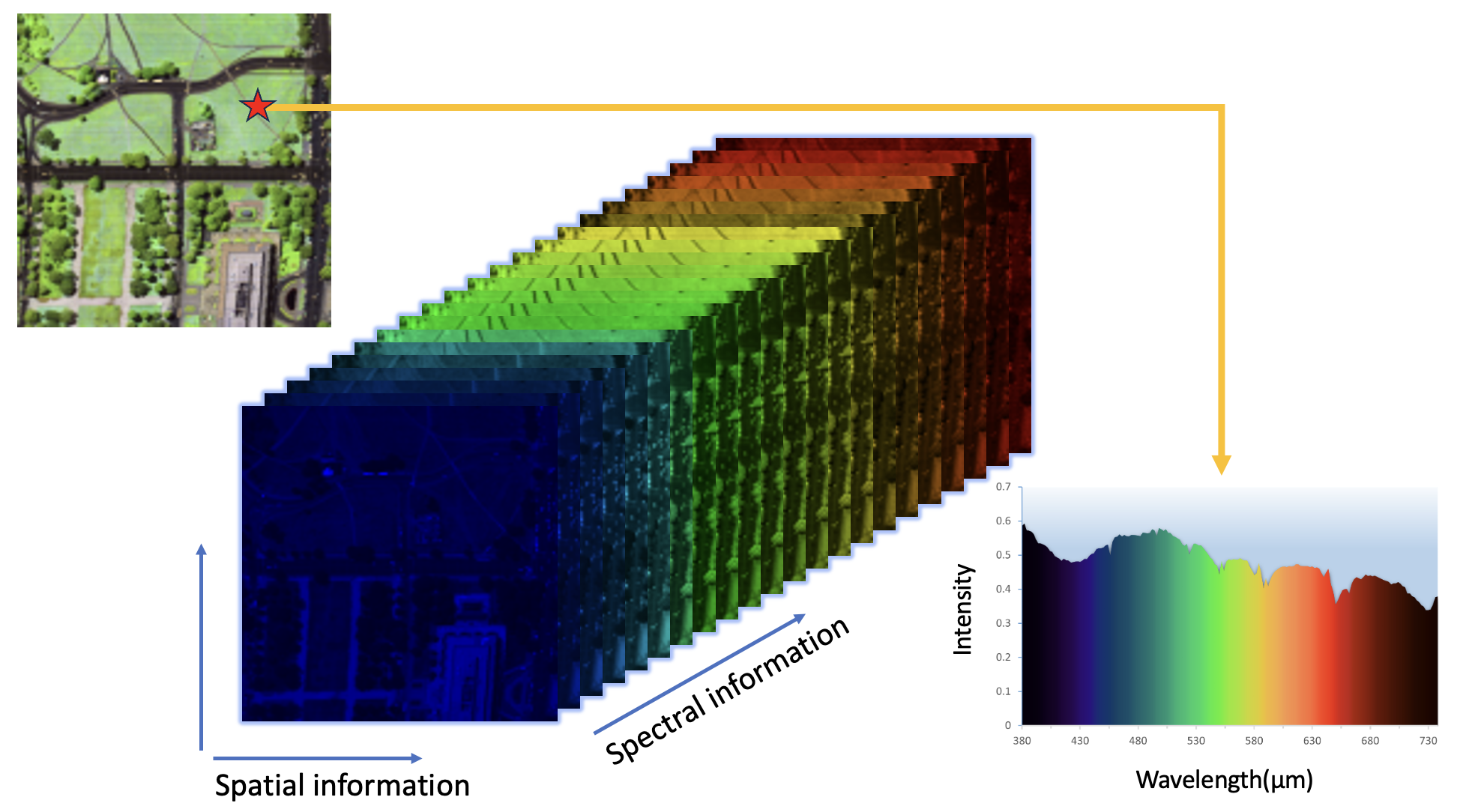
Figure 1: An illustrative figure of an HSI.

HSIs are often contaminated by Gaussian noise, impulse noise, stripe noise, dead line noise, and so on. Mathematically, a noisy HSI $\mathcal{D}\in\mathbb{R}^{I_{1}\times I_{2}\times I_{3}}$ can be expressed as

$$\mathcal{D}=\mathcal{L}+\mathcal{S}+\mathcal{N},$$

where $\mathcal{L}\in\mathbb{R}^{I_{1}\times I_{2}\times I_{3}}$ represents the clean HSI, $\mathcal{S}\in\mathbb{R}^{I_{1}\times I_{2}\times I_{3}}$ represents the sparse noises such as impulse noise, stripe noise and dead line noise, and $\mathcal{N}\in\mathbb{R}^{I_{1}\times I_{2}\times I_{3}}$ represents Gaussian noise.

To remove Gaussian noise in HSIs, many methods have been proposed. Conventional 2-D methods [9, 12], processing HSIs band by band, do not fully utilize the strong correlation between adjacent bands. 3-D methods such as Block-matching 4-D filtering (BM4D) [24], spectral-spatial adaptive hyperspectral total variation (SSAHTV) model [40], and sparse representation methods [45, 35] incorporate both spatial and spectral information and outperform conventional methods. However, those methods may fail to remove non-Gaussian noise.

In real-world scenarios, HSIs are often contaminated by more than one type of noises due to atmospheric effects and instrument noise. Various methods have been proposed to remove the mixed noise, including low-rank matrix based methods, low-rank tensor based methods, and deep learning based methods. Low-rank matrix based methods [16, 42] reshape an HSI into a matrix and impose low-rankness on the reshaped HSI. Zhang et al. [43] formulated the HSI denoising problem as a low-rank matrix factorization problem and solved it by the “Go Decomposition” algorithm; Zhang et al. [42] proposed a double low-rank matrix decomposition which utilized the $\ell_{1}$ norm for the impulse noise and the matrix nuclear norm for stripes, and adopted augmented Lagrangian method (ALM) to solve the model; Yang et al. [38] also used double low-rankness, but added spatial-spectral total variation (SSTV) to the model and performed the decomposition on full band blocks (FBBs) rather than the entire HSI.

Low-rank tensor based methods [18, 10, 26, 14, 46] view HSIs as tensors and perform tensor low-rank decompositions while preserving the spatial-spectral correlations. Wang et al. [32] used Tucker tensor decomposition and an anisotropic SSTV regularization to characterize the piece-wise smooth structures of the HSI; Chen et al.  [8] proposed a low-rank tensor decomposition (LRTD) method, which utilized the higher-order singular value decomposition (HOSVD) for low-rankness and the matrix $\ell_{2,1}$ norm for characterizing the stripes, and adopted ALM for solving the optimization model; Cao et al. [5] proposed a subspace-based nonlocal low-rank and sparse factorization (SNLRSF) method for removing mixed noise in HSI, which conducted nonlocal low-rank factorization via successive singular value decomposition (SVD); Xiong et al. [36] proposed the LRTFL0 method using low-rank block term decomposition and spectral-spatial $\ell_{0}$ gradient regularization to achieve gradient smoothness.

Recently, some deep neural networks [4, 41, 34] have been proposed to denoise HSIs. Quasi-Recurrent Neural Networks (QRNN) [4] combined recurrent neural networks (RNN) with convolutional neural networks (CNN); the 3-D version of QRNN (QRNN3D) [34] can effectively embed the correlation of HSIs; CNN can also be used as a denoiser in a plug-and-play fashion for HSI denoising [30].

To remove Gaussian noise and stripes simultaneously, we propose an optimization model utilizing low-rank tensor regularization and a group sparsity measure, which is formulated as follows

(1) $$\begin{split}\min_{\begin{subarray}{c}\mathcal{S},[{X}_{1}],[{X}_{2}],\\ [{X}_{3}],[\mathcal{G}],\mathcal{L}\end{subarray}}\quad&\frac{\delta}{2}\|\mathbf{R}(\mathcal{L}+\mathcal{S}-\mathcal{D})\|_{F}^{2}+\gamma\|\sqrt{\mathcal{W}_{\mathbf{R}}}\odot\mathcal{S}\|^{p}_{2,p}+\|[\mathcal{G}]\|_{1,w}\\ &+\frac{1}{2}\|\mathbf{R}(\mathcal{L})-[\mathcal{G}]\times_{1}[X_{1}]\times_{2}[X_{2}]\times_{3}[X_{3}]\|^{2}_{F}\\ \mbox{s.t. }&[{X}_{i}]^{\top}[{X}_{i}]=[\mathbf{I}_{n_{i}}],\quad i=1,2,3,\end{split}$$

where

• $\mathcal{S},\mathcal{L}\in\mathbb{R}^{I_{1}\times I_{2}\times I_{3}}$, $[\mathcal{G}]\in\mathbb{R}^{n_{1}\times n_{2}\times n_{3}\times N}$ and $[X_{i}]\in\mathbb{R}^{m_{i}\times n_{i}\times N}$, $m_{i}\geq n_{i}$, $i=1,2,3$;

• $\mathbf{R}:\mathbb{R}^{I_{1}\times I_{2}\times I_{3}}\to\mathbb{R}^{m_{1}\times m_{2}\times m_{3}\times N}$ denotes the similar blocks extraction operator, and $\mathbf{R}^{\top}:$ $\mathbb{R}^{m_{1}\times m_{2}\times m_{3}\times N}\to\mathbb{R}^{I_{1}\times I_{2}\times I_{3}}$ denotes the transpose of $\mathbf{R}$ satisfying $\langle\mathbf{R}(\mathcal{L}),[\mathcal{Y}]\rangle=\langle\mathcal{L},\mathbf{R}^{\top}([\mathcal{Y}])\rangle$ for any $\mathcal{L}\in\mathbb{R}^{I_{1}\times I_{2}\times I_{3}}$, $[\mathcal{Y}]\in\mathbb{R}^{m_{1}\times m_{2}\times m_{3}\times N}$;

• $\mathcal{W}_{\mathbf{R}}\in\mathbb{R}_{++}^{I_{1}\times I_{2}\times I_{3}}$ denotes a weight tenor such that the component-wise multiplication with $\mathcal{W}_{\mathbf{R}}$ is an equivalent operation of $\mathbf{R}^{\top}\mathbf{R}$, i.e., $\mathcal{W}_{\mathbf{R}}\odot\operatorname{Id}=\mathbf{R}^{\top}\mathbf{R}$, $\odot$ denotes the component-wise multiplication, $\operatorname{Id}$ denotes the identity mapping on $\mathbb{R}^{I_{1}\times I_{2}\times I_{3}}$ and $\sqrt{\mathcal{W}_{\mathbf{R}}}$ denotes the component-wise square root of $\mathcal{W}_{\mathbf{R}}$, i.e., the $(i_{1},i_{2},i_{3})$-th entry of $\sqrt{\mathcal{W}_{\mathbf{R}}}$ is equal to $\sqrt{(\mathcal{W}_{\mathbf{R}})_{i_{1}i_{2}i_{3}}}$;

• $\|\sqrt{\mathcal{W}_{\mathbf{R}}}\odot\mathcal{S}\|_{2,p}$ denotes the weighted tensor $\ell_{2,p}$ (quasi-)norm with $p\in(0,1)$ of a third order tensor $\hat{\mathcal{S}}=\sqrt{\mathcal{W}_{\mathbf{R}}}\odot\mathcal{S}$ defined by

  (2) $$\|\hat{\mathcal{S}}\|_{2,p}=\left(\sum_{i_{3}=1}^{I_{3}}\sum_{i_{2}=1}^{I_{2}}\|\hat{s}_{:i_{2}i_{3}}\|^{p}_{2}\right)^{\frac{1}{p}}=\left(\sum_{i_{3}=1}^{I_{3}}\sum_{i_{2}=1}^{I_{2}}\left(\sum_{i_{1}=1}^{I_{1}}\hat{s}_{i_{1}i_{2}i_{3}}^{2}\right)^{\frac{p}{2}}\right)^{\frac{1}{p}},$$

  and the tensor $\ell_{2,p}$ norm is exactly equal to the matrix $\ell_{2,p}$ norm of the unfolding matrix of $\hat{\mathcal{S}}$ along the first dimension, i.e., $\|\hat{\mathcal{S}}\|_{2,p}=\|\hat{S}_{(1)}\|_{2,p}$;

• $[\mathcal{G}]\times_{1}[X_{1}]\times_{2}[X_{2}]\times_{3}[X_{3}]$ denotes an independent 3-D HOSVD with $[\mathcal{G}]$ being the independent core tensors and $[X_{i}]$ being the independent mode-$i$ factor matrices, $i=1,2,3$, and $[X_{i}]$ is independently orthogonal, i.e., $[{X}_{i}]^{\top}[{X}_{i}]=[\mathbf{I}_{n_{i}}]$, with $\mathbf{I}_{n_{i}}$ representing the identity matrix of size $n_{i}\times n_{i}$;

• $\|[\mathcal{G}]\|_{1,w}$ denotes the weighted tensor (component-wise) $\ell_{1}$ norm for a fourth order tensor $[\mathcal{G}]$ defined by

  (3) $$\|[\mathcal{G}]\|_{1,w}=\sum_{j=1}^{N}w_{j}\|[\mathcal{G}]^{(j)}\|_{1},$$

  with a weight vector $w\in\mathbb{R}^{N}_{++}$.

Model (1) is a nonconvex nonsmooth minimization problem with orthogonal constraints. In particular, the first term of model (1) is a data fidelity term to remove Gaussian noise, the second term is a group sparsity measure to remove sparse noises with linear structures, and the last two terms are the sparsity-enhanced nonlocal low-rank tensor regularization terms. A detailed description of the model for HSI denoising and destriping will be presented in section 5, with the formulations for $\mathbf{R}$, $\mathbf{R}^{\top}$ and $\mathcal{W}_{\mathbf{R}}$.

Our main contributions are summarized as follows:

• We propose a novel model to remove mixed noise in HSIs using a new sparsity-enhanced low-rank regularization and a tensor $\ell_{2,p}$ norm with $p\in(0,1)$. For removing Gaussian noise, a fourth order tensor is formed by nonlocal similar FBBs via the extraction operator $\mathbf{R}$ and is further regularized on its low-rankness using independent 3-D HOSVD with sparsity enhancement on its core tensors to prompt more low-rankness. The tensor $\ell_{2,p}$ norm for removing the dead lines and stripes is extended from the matrix $\ell_{2,p}$ norm. Some new mathematical results on finding the proximal operator of the tensor $\ell_{2,p}$ norm are also presented. We show that model (1) has a nonempty and bounded solution set.

• We propose a proximal block coordinate descent (P-BCD) algorithm for solving problem (1). Each subproblem of the P-BCD algorithm has an exact form solution, which either has a closed-form solution or is easy to compute. We define the first-order stationary point of model (1) using three equalities of substationarity, symmetry, and feasibility for orthogonal constraints. We prove that any accumulation point of the sequence generated by P-BCD algorithm is a first-order stationary point.

• We show the proposed nonlocal low-rank tensor regularized $\ell_{2,p}$ (NLTL2p) approach for HSI denoising and destriping can outperform other state-of-the-art methods including a deep learning based method on the numerical experiments tested on both simulated and real HSI datasets.

The rest of this paper is organized as follows. In section 2, we present some notations and preliminaries for tensors, nonconvex nonsmooth optimization, manifold optimization, and independent 3-D HOSVD. For solving model (1), we propose a P-BCD method in section 3 and conduct its convergence analysis in section 4. Next, we apply the proposed NLTL2p approach to HSI denoising and destriping in section 5 and conduct experiments on simulated and real HSI data in section 6. The concluding remarks are given in section 7.

2 Notations and Preliminaries

In this section, we first present the notations for tensors, nonconvex nonsmooth optimization, and manifold optimization, then we introduce some notations and preliminaries for the independent 3-D HOSVD.

2.1 Notations

First, we introduce the notations for tensors. For a third order tensor $\mathcal{X}\in\mathbb{R}^{I_{1}\times I_{2}\times I_{3}}$, we let $x_{i_{1}i_{2}i_{3}}$ denote its $(i_{1},i_{2},i_{3})$-th entry, let $x_{:i_{2}i_{3}}$ denote its $(i_{2},i_{3})$-th mode-$1$ fiber and let $X_{::i_{3}}$ denote its $i_{3}$-th frontal slice. And $\mathcal{X}\in\mathbb{R}^{I_{1}\times I_{2}\times I_{3}}_{++}$ means all its entries are positive. The mode-$k$ unfolding of a third order tensor $\mathcal{X}$ is denoted as $X_{(k)}={\rm unfold}_{(k)}(\mathcal{X})$, which is the process to linearize all indexes except index $k$. The dimensions of $X_{(k)}$ are $I_{k}\times\prod^{3}_{j=1,j\neq k}I_{j}$. An element $x_{i_{1}i_{2}i_{3}}$ of $\mathcal{X}$ corresponds to the position of $(i_{k},j)$ in matrix $X_{(k)}$, where $j=1+\sum^{3}_{l=1,l\neq k}(i_{l}-1)\prod^{l-1}_{m=1,m\neq k}I_{m}$. And the inverse process of the mode-$k$ unfolding of a tensor $\mathcal{X}$ is denoted by $\mathcal{X}={\rm fold}_{(k)}(X_{(k)})$.

The (component-wise) $\ell_{1}$ norm and Frobenius norm of $\mathcal{X}$ are given by

$$\|\mathcal{X}\|_{1}: =\textstyle\sum_{i_{1}=1}^{I_{1}}\sum_{i_{2}=1}^{I_{2}}\sum_{i_{3}=1}^{I_{3}}|x_{i_{1}i_{2}i_{3}}|,$$

$$\|\mathcal{X}\|_{F}: =(\textstyle\sum_{i_{1}=1}^{I_{1}}\sum_{i_{2}=1}^{I_{2}}\sum_{i_{3}=1}^{I_{3}}|x_{i_{1}i_{2}i_{3}}|^{2})^{\frac{1}{2}}.$$

Next, we provide the definitions for (limiting) subdifferentials and proximal operators. Let $f:\mathbb{R}^{d}\to(-\infty,+\infty]$ be a proper and lower semicontinuous function with a finite lower bound. The (limiting) subdifferential of $f$ at $x\in\operatorname{dom}f:=\{x\in\mathbb{R}^{d}|f(x)<\infty\}$, denoted by $\partial f(x)$, is defined as

$$\partial f(x)\!:=\{u\in\mathbb{R}^{d}|\exists x^{k}\to x,f(x^{k})\to f(x)\text{ and }u^{k}\to u\text{ with }u^{k}\in\hat{\partial}f(x^{k})\mbox{ as }k\to\infty\},$$

where $\hat{\partial}f(x)$ denotes the Fréchet subdifferential of $f$ at $x\in\operatorname{dom}f$, which is the set of all $u\in\mathbb{R}^{d}$ satisfying

(4) $$\begin{split}\underset{y\neq x,y\rightarrow x}{\lim\inf}\frac{f(y)-f(x)-\langle u,y-x\rangle}{\|y-x\|}\geq 0.\end{split}$$

One can also observe that $\{u\in\mathbb{R}^{d}|\exists x^{k}\to x,f(x^{k})\to f(x)\text{ and }u^{k}\to u\text{ with }u^{k}\in\partial f(x^{k})\mbox{ as }k\to\infty\}\subseteq\partial f(x)$. Next, the proximal operator of $f$ with parameter $\lambda>0$ evaluated at $x\in\mathbb{R}^{d}$, denoted as $\text{prox}_{\lambda f}(x)$, is defined as

$$\text{prox}_{\lambda f}(x):=\underset{u\in\mathbb{R}^{d}}{\arg\!\min}\left[f(u)+\frac{1}{2\lambda}\|u-x\|_{2}^{2}\right].$$

Note that $\text{prox}_{\lambda f}$ is a single-valued map, if $f$ is a convex function. However, when $f$ is nonconvex, $\text{prox}_{\lambda f}(x)$ may have multiple points.

Also, we set $\mathbb{S}_{m,n}:=\{X\in\mathbb{R}^{m\times n}|X^{\top}X=\mathbf{I}_{n}\}$ as the Stiefel manifold with $m\geq n$ and set $\mathcal{T}_{X}\mathbb{S}_{m,n}:=\{Y\in\mathbb{R}^{m\times n}|Y^{\top}X+X^{\top}Y=0\}$ as the tangent space of Stiefel manifold at $X\in\mathbb{R}^{m\times n}$. We also set the Riemannian metric on Stiefel manifold as the metric induced from the Euclidean inner product. Then according to [1], the Riemannian gradient of a smooth function $f$ at $X$ is given by

$$\operatorname{grad}f(X):=\operatorname{Proj}_{\mathcal{T}_{X}\mathbb{S}_{m,n}}(\nabla f(X)),$$

where $\operatorname{Proj}_{\mathcal{T}_{X}\mathbb{S}_{m,n}}(Y):=(\mathbf{I}_{m}-XX^{\top})Y+\frac{1}{2}X(X^{\top}Y-Y^{\top}X)$.

2.2 Independent 3-D HOSVD

We introduce the definition of a 3-D HOSVD and then define an independent 3-D HOSVD using the notation of $[\,\cdot\,]$. For a third order tensor $\mathcal{Y}\in\mathbb{R}^{m_{1}\times m_{2}\times m_{3}}$, the (truncated) 3-D HOSVD of $\mathcal{Y}$ is to approximate $\mathcal{Y}$ in the following form

(5) $$\mathcal{Y}\approx\mathcal{G}\times_{1}{X}_{1}\times_{2}{X}_{2}\times_{3}{X}_{3},$$

where $\mathcal{G}\in\mathbb{R}^{n_{1}\times n_{2}\times n_{3}}$ is the core tensor, and ${X}_{i}\in\mathbb{R}^{m_{i}\times n_{i}}$ is the $i$-th factor matrix such that ${X}_{i}^{\top}{X}_{i}=\mathbf{I}_{n_{i}}$. Note that $m_{i}\geq n_{i}$ and ${X}_{i}$ belongs to a Stiefel manifold, i.e., ${X}_{i}\in\mathbb{S}_{m_{i},n_{i}}$. By imposing orthogonality on the factor matrices, the decomposition in (5) can inherit some nice properties from the matrix SVD. For example, the core tensor can have the all-orthogonality and the ordering property [7].

When a fourth order tensor has little correlation across the last mode, we view the fourth order tensor as a stack of independent third order tensors. Using the notation of $[\,\cdot\,]$, we denote such a fourth order tensor as $[\mathcal{Y}]\in\mathbb{R}^{m_{1}\times m_{2}\times m_{3}\times N}$ and its $j$-th third order tensor as $[\mathcal{Y}]^{(j)}\in\mathbb{R}^{m_{1}\times m_{2}\times m_{3}}$, $j=1,2,\dots,N$. Also, a stack of independent matrices is denoted as $[X]\in\mathbb{R}^{m\times n\times N}$. And we say $[X]$ is independently orthogonal if $[{X}]^{\top}[{X}]=[\mathbf{I}_{n}]$, meaning $([{X}]^{(j)})^{\top}[{X}]^{(j)}=\mathbf{I}_{n}$, or equivalently $[X]\in[\mathbb{S}_{m,n}]$, meaning $[X]^{(j)}\in\mathbb{S}_{m,n}$. Then we define an independent (truncated) 3-D HOSVD of $[\mathcal{Y}]$ as

$$[\mathcal{Y}]\approx[\mathcal{G}]\times_{1}[{X}_{1}]\times_{2}[{X}_{2}]\times_{3}[{X}_{3}],$$

where $[\mathcal{G}]\in\mathbb{R}^{n_{1}\times n_{2}\times n_{3}\times N}$, $[X_{i}]\in\mathbb{R}^{m_{i}\times n_{i}\times N}$, and $[\mathcal{Y}]^{(j)}\approx[\mathcal{G}]^{(j)}\times_{1}[{X}_{1}]^{(j)}\times_{2}[{X}_{2}]^{(j)}\times_{3}[{X}_{3}]^{(j)}$ with $([{X}_{i}]^{(j)})^{\top}[{X}_{i}]^{(j)}=\mathbf{I}_{n_{i}}$, $i=1,2,3$, $j=1,2,\dots,N$. Similarly, we extend the notation of $[\,\cdot\,]$ to other operations acting on independent tensors. That is, performing an operation on independent tensors means performing the operation on each lower order tensor independently. For example, performing the mode-$k$ unfolding on $[\mathcal{G}]$, denoted as $[\mathcal{G}]_{[(k)]}$, means independently performing $[\mathcal{G}]^{(j)}_{(k)}$ for each $j$, which is the mode-$k$ unfolding on $[\mathcal{G}]^{(j)}$.

3 Proximal Block Coordinate Descent Algorithm

The proposed nonlocal low-rank tensor model (1) is a nonconvex and nonsmooth optimization problem over Stiefel manifolds. In this section, we propose a P-BCD algorithm for solving model (1).

Let $\Phi$ denote the objective function of model (1) defined by

$$\Phi(\mathcal{S},[{X}_{1}],[{X}_{2}],[{X}_{3}],[\mathcal{G}],\mathcal{L}):= \frac{\delta}{2}\|\mathbf{R}(\mathcal{L}+\mathcal{S}-\mathcal{D})\|_{F}^{2}+\gamma\varphi\left(\sqrt{\mathcal{W}_{\mathbf{R}}}\odot\mathcal{S}\right)+\psi([\mathcal{G}])$$

$$+\frac{1}{2}H([X_{1}],[X_{2}],[X_{3}],[\mathcal{G}],\mathcal{L}),$$

where $\varphi(\sqrt{\mathcal{W}_{\mathbf{R}}}\odot\mathcal{S})=\|\sqrt{\mathcal{W}_{\mathbf{R}}}\odot\mathcal{S}\|_{2,p}^{p}$, $\psi([\mathcal{G}])=\|[\mathcal{G}]\|_{1,w}$, and

(6) $$H([X_{1}],[X_{2}],[X_{3}],[\mathcal{G}],\mathcal{L}):=\frac{1}{2}\|\mathbf{R}(\mathcal{L})-[\mathcal{G}]\times_{1}[X_{1}]\times_{2}[X_{2}]\times_{3}[X_{3}]\|^{2}_{F}.$$

Then the P-BCD algorithm is summarized as follows:

$$\mathcal{S}^{k+1} \in\underset{\mathcal{S}}{\arg\!\min}\;\Phi(\mathcal{S},[{X}_{1}^{k}],[{X}_{2}^{k}],[{X}_{3}^{k}],[\mathcal{G}^{k}],\mathcal{L}^{k})+\frac{\alpha_{\mathcal{S}}}{2}\|\sqrt{\mathcal{W}_{\mathbf{R}}}\odot(\mathcal{S}-\mathcal{S}^{k})\|^{2}_{F},$$

$$[{X}_{1}^{k+1}] \in\underset{[{X}_{1}]\in[\mathbb{S}_{m_{1},n_{1}}]}{\arg\!\min}\!\Phi(\mathcal{S}^{k+1},[{X}_{1}],[{X}_{2}^{k}],[{X}_{3}^{k}],[\mathcal{G}^{k}],\mathcal{L}^{k})+\frac{\alpha_{X}}{2}\|[{X}_{1}]-[{X}_{1}^{k}]\|^{2}_{F},$$

$$[{X}_{2}^{k+1}] \in\underset{[{X}_{2}]\in[\mathbb{S}_{m_{2},n_{2}}]}{\arg\!\min}\!\Phi(\mathcal{S}^{k+1},[{X}_{1}^{k+1}],[{X}_{2}],[{X}_{3}^{k}],[\mathcal{G}^{k}],\mathcal{L}^{k})+\frac{\alpha_{X}}{2}\|[{X}_{2}]-[{X}_{2}^{k}]\|^{2}_{F},$$

$$[{X}_{3}^{k+1}] \in\underset{[{X}_{3}]\in[\mathbb{S}_{m_{3},n_{3}}]}{\arg\!\min}\!\Phi(\mathcal{S}^{k+1},[{X}_{1}^{k+1}],[{X}_{2}^{k+1}],[{X}_{3}],[\mathcal{G}^{k}],\mathcal{L}^{k})+\frac{\alpha_{X}}{2}\|[{X}_{3}]-[{X}_{3}^{k}]\|^{2}_{F},$$

$$[\mathcal{G}^{k+1}] =\underset{[\mathcal{G}]}{\arg\!\min}\;\Phi(\mathcal{S}^{k+1},[{X}_{1}^{k+1}],[{X}_{2}^{k+1}],[{X}_{3}^{k+1}],[\mathcal{G}],\mathcal{L}^{k})+\frac{\alpha_{\mathcal{G}}}{2}\|[\mathcal{G}]-[\mathcal{G}^{k}]\|^{2}_{F},$$

$$\mathcal{L}^{k+1} =\underset{\mathcal{L}}{\arg\!\min}\;\Phi(\mathcal{S}^{k+1},[{X}_{1}^{k+1}],[{X}_{2}^{k+1}],[{X}_{3}^{k+1}],[\mathcal{G}^{k+1}],\mathcal{L}),$$

where parameters $\alpha_{\mathcal{S}},\alpha_{X},\alpha_{\mathcal{G}}>0$.

In the following, we present the details for computing each update. We will conduct a convergence analysis for the proposed P-BCD algorithm in the next section.

3.1 The update of $\mathcal{S}$

Recall that

$$\|\mathbf{R}(\mathcal{L})\|_{F}^{2}=\langle\mathcal{L},\mathbf{R}^{\top}\mathbf{R}(\mathcal{L})\rangle_{F}=\langle\mathcal{L},\mathcal{W}_{\mathbf{R}}\odot\mathcal{L}\rangle_{F}=\|\sqrt{\mathcal{W}_{\mathbf{R}}}\odot\mathcal{L}\|_{F}^{2}.$$

Then $\mathcal{S}^{k+1}$ is computed by

$$\mathcal{S}^{k+1}\in\underset{\mathcal{S}}{\arg\!\min}\;\tilde{\gamma}\varphi\left(\sqrt{\mathcal{W}_{\mathbf{R}}}\odot\mathcal{S}\right)+\frac{1}{2}\left\|\sqrt{\mathcal{W}_{\mathbf{R}}}\odot\left[\mathcal{S}-(\mathcal{S}^{k}-\tilde{\alpha}_{\mathcal{S}}\left(\mathcal{S}^{k}+\mathcal{L}^{k}-\mathcal{D})\right)\right]\right\|_{F}^{2},$$

where $\tilde{\gamma}=\frac{\gamma}{\delta+\alpha_{\mathcal{S}}}$ and $\tilde{\alpha}_{\mathcal{S}}=\frac{\delta}{\delta+\alpha_{\mathcal{S}}}$. Rescaling $\mathcal{S}$ using $\sqrt{\mathcal{W}_{\mathbf{R}}}\odot$, $\mathcal{S}^{k+1}$ can be written in terms of the proximal operator of $\varphi$ as follows

(7) $$\mathcal{S}^{k+1}\in\left(\sqrt{\mathcal{W}_{\mathbf{R}}}\right)^{-1}\odot\operatorname{prox}_{\tilde{\gamma}\varphi}\left[\sqrt{\mathcal{W}_{\mathbf{R}}}\odot\left(\mathcal{S}^{k}-\tilde{\alpha}_{\mathcal{S}}\left(\mathcal{S}^{k}+\mathcal{L}^{k}-\mathcal{D}\right)\right)\right],$$

where the $(i_{1},i_{2},i_{3})$-th entry of $\left(\sqrt{\mathcal{W}_{\mathbf{R}}}\right)^{-1}$ is equal to $1/\sqrt{(\mathcal{W}_{\mathbf{R}})_{i_{1}i_{2}i_{3}}}$.

3.2 The update of $[X_{i}]$

Before we solve the optimization subproblem in terms of $[X_{i}]$ over independent Stiefel manifolds, we can rewrite its objective function using the following useful fact for unfolding of tensors

$$\mathcal{Y}=\mathcal{G}\times_{i}X\mbox{ if and only if }{Y}_{(i)}=XG_{(i)}.$$

Then by applying $X\in\mathbb{S}_{m,n}$, the Frobenious norm of tensors can be rewritten into the Frobenious norm of matrices

$$\|\mathcal{G}\times_{i}X-\mathcal{L}\|_{F}^{2}= \|XG_{(i)}-L_{(i)}\|_{F}^{2}$$

(8) $$= \|G_{(i)}\|_{F}^{2}-2\langle XG_{(i)},L_{(i)}\rangle+\|L_{(i)}\|_{F}^{2},$$

where $G_{(i)}$ and $L_{(i)}$ denote the mode-$i$ unfolding of $\mathcal{G}$ and $\mathcal{L}$, respectively. Since $\langle XG_{(i)},L_{(i)}\rangle=\langle X,L_{(i)}G_{(i)}^{\top}\rangle$ and $\|X\|_{F}^{2}=n$, minimizing $\|\mathcal{G}\times_{i}X-\mathcal{L}\|_{F}^{2}$ over $X$ on the Stiefel manifold is equivalent to minimizing $\|X-L_{(i)}G_{(i)}^{\top}\|_{F}^{2}$ over the Stiefel manifold. Hence, $[X_{i}^{k+1}]$ can be computed via the projection of unfolding matrices onto the Stiefel manifolds independently as follows

(9) $$[X_{i}^{k+1}]\in\operatorname{Proj}_{[\mathbb{S}_{m_{i},n_{i}}]}\left([X_{i}^{k}]-\tilde{\alpha}_{X}\left([X_{i}^{k}]-[P_{i}^{k}][Q_{i}^{k}]^{\top}\right)\right),$$

where $[P_{i}^{k}]=(\mathbf{R}(\mathcal{L}^{k}))_{[(i)]}$, $[Q_{1}^{k}]=\left([\mathcal{G}^{k}]\times_{2}[X^{k}_{2}]\times_{3}[X^{k}_{3}]\right)_{[(1)]}$, $[Q_{2}^{k}]=\big{(}[\mathcal{G}^{k}]\times_{1}[X_{1}^{k+1}]$ $\times_{3}[X^{k}_{3}]\big{)}_{[(2)]}$, $[Q_{3}^{k}]=\left([\mathcal{G}^{k}]\times_{1}[X^{k+1}_{1}]\times_{2}[X^{k+1}_{2}]\right)_{[(3)]}$, and parameter $\tilde{\alpha}_{X}=\frac{1}{1+\alpha_{X}}$.

In the following, we present a lemma for finding the projection onto a Stiefel manifold, which is given in Theorem 4.1 in [17] and proved in [2].

Lemma 3.1.

[17, 2] Given $A\in\mathbb{R}^{m\times n}$, $m\geq n$, consider the following Stiefel manifold projection problem

(10) $$\begin{split}&\min_{X\in\mathbb{R}^{m\times n}}\|X-A\|^{2}_{F}\\ &{\rm s.t.}\quad X^{\top}X=\mathbf{I}_{n}.\end{split}$$

Then the set of optimal solutions of problem (10), denoted as $\Omega^{*}(A)$, is given by

$$\Omega^{*}(A)=\{UV^{\top}| A=U\Sigma V^{\top},U\in\mathbb{R}^{m\times n},\Sigma\in\mathbb{R}^{n\times n},V\in\mathbb{R}^{n\times n}$$

$$\text{ such that }U^{\top}U=V^{\top}V=\mathbf{I}_{n}\text{ and }\Sigma=\operatorname{Diag}(\sigma(A))\},$$

where $U\Sigma V^{\top}$ is a reduced SVD of $A$ and $\sigma(A)\in\mathbb{R}^{n}$ is a vector of all the singular values of $A$. In particular, if $A$ is of full column rank $n$, then $\Omega^{*}(A)$ is a singleton.

According to Lemma 3.1, problem (10) has a closed form solution, even though it may have multiple solutions when the given matrix does not have full column rank. Hence, if $[U][\Sigma][V]^{\top}$ is an independent reduced SVD of $[A]\in\mathbb{R}^{m\times n\times N}$, then $[U][V]^{\top}\in\operatorname{Proj}_{[\mathbb{S}_{m,n}]}([A])$.

3.3 The update of $[\mathcal{G}]$

The subproblem for updating $[\mathcal{G}]$ can be reformulated by using the following property that for any $X\in\mathbb{S}_{m,n}$, $m\geq n$,

$$\|\mathcal{G}\times_{i}X-\mathcal{L}\|_{F}^{2}$$

$$= \|G_{(i)}-X^{\top}L_{(i)}\|_{F}^{2}-\|X^{\top}L_{(i)}\|_{F}^{2}+\|L_{(i)}\|_{F}^{2}$$

$$= \|\mathcal{G}-\mathcal{L}\times_{i}X^{\top}\|_{F}^{2}-\|\mathcal{L}\times_{i}X^{\top}\|_{F}^{2}+\|\mathcal{L}\|_{F}^{2},$$

which is derived from (8) and the constraint that $X^{\top}X=\mathbf{I}_{n}$. Then $[\mathcal{G}^{k+1}]$ can be computed by

(11) $$[\mathcal{G}^{k+1}]=\operatorname{prox}_{\tilde{\alpha}_{\mathcal{G}}\psi}\left([\mathcal{G}^{k}]-\tilde{\alpha}_{\mathcal{G}}([\mathcal{G}^{k}]-[\mathcal{O}^{k+1}])\right),$$

where $[\mathcal{O}^{k+1}]=\mathbf{R}(\mathcal{L}^{k})\times_{1}[X_{1}^{k+1}]^{\top}\times_{2}[X_{2}^{k+1}]^{\top}\times_{3}[X_{3}^{k+1}]^{\top}$, and $\tilde{\alpha}_{\mathcal{G}}=\frac{1}{1+\alpha_{\mathcal{G}}}$.

3.4 The update of $\mathcal{L}$

After computing $[X_{i}^{k+1}]$ and $[\mathcal{G}^{k+1}]$, we can obtain the approximated low-rank group tensor, denoted as $[\mathcal{Y}^{k+1}]$, as follows

(12) $$[\mathcal{Y}^{k+1}]=[\mathcal{G}^{k+1}]\times_{1}[X_{1}^{k+1}]\times_{2}[X_{2}^{k+1}]\times_{3}[X_{3}^{k+1}].$$

Then $\mathcal{L}^{k+1}$ can be computed in a unique closed form as follows

(13) $$\mathcal{L}^{k+1}= \tilde{\delta}\mathcal{W}_{\mathbf{R}}^{-1}\odot\mathbf{R}^{\top}([\mathcal{Y}^{k+1}])+(1-\tilde{\delta})(\mathcal{D}-\mathcal{S}^{k+1}),$$

where parameter $\tilde{\delta}=\frac{1}{1+\delta}$ and $\mathcal{W}_{\mathbf{R}}^{-1}$ denotes the component-wise inverse of $\mathcal{W}_{\mathbf{R}}$, i.e., the $(i_{1},i_{2},i_{3})$-th entry of $\mathcal{W}_{\mathbf{R}}^{-1}$ is equal to $1/(\mathcal{W}_{\mathbf{R}})_{i_{1}i_{2}i_{3}}$.

All in all, the proposed P-BCD algorithm for model (1) is summarized in Algorithm 1.

Algorithm 1 Proximal BCD (P-BCD) algorithm for model (1)

1:  Initialize $(\mathcal{S}^{0},[{X}_{1}^{0}],[{X}_{2}^{0}],[{X}_{3}^{0}],[\mathcal{G}^{0}],\mathcal{L}^{0})$ with $[{X}_{i}^{0}]\in[\mathbb{S}_{m_{i},n_{i}}]$;

2:  Set the tensor extraction operator $\mathbf{R}$;

3:  Set parameters $\alpha_{\mathcal{S}},\alpha_{X},\alpha_{\mathcal{G}}>0$;

4:  Set $k=0$.

5:  repeat

6:     Compute $\mathcal{S}^{k+1}$ by (7);

7:     Compute $[X_{i}^{k+1}]$ by (9), $i=1,2,3$;

8:     Compute $[\mathcal{G}^{k+1}]$ by (11);

9:     Compute $\mathcal{L}^{k+1}$ by (13);

10:     $k\leftarrow k+1$.

11:  until the stopping criterion is met.

11:  $(\mathcal{S}^{k},[{X}_{1}^{k}],[{X}_{2}^{k}],[{X}_{3}^{k}],[\mathcal{G}^{k}],\mathcal{L}^{k})$.

4 Convergence Analysis of The P-BCD Algorithm

The proposed P-BCD algorithm aims to solve a particular optimization problem of the form as in (1). An optimal solution of each subproblem in our algorithm is obtained as shown in the previous subsections. The P-BCD algorithm can be viewed as a special variant of the proximal alternating linearization minimization (PALM) [3] extended for multiple blocks or the block coordinate update with prox-linear approximation [37], called the block prox-linear method. In the following, we present the convergence results of the P-BCD algorithm.

Let $\mathcal{Z}:=(\mathcal{S},[X_{1}],[X_{2}],[X_{3}],[\mathcal{G}],\mathcal{L})$. First, we define the first-order optimality condition of the orthogonal constrained optimization problem as in (1). The point $\bar{\mathcal{Z}}:=(\bar{\mathcal{S}},[\bar{X}_{1}],[\bar{X}_{2}],[\bar{X}_{3}],[\bar{\mathcal{G}}],\bar{\mathcal{L}})$ is a first-order stationary point of problem (1) if $0\in\partial\Phi(\bar{\mathcal{Z}})$, that is,

$${0}\in\delta\mathcal{W}_{\mathbf{R}}\odot(\bar{\mathcal{L}}+\bar{\mathcal{S}}-\mathcal{D})+\gamma\sqrt{\mathcal{W}_{\mathbf{R}}}\odot\partial\varphi(\sqrt{\mathcal{W}_{\mathbf{R}}}\odot\bar{\mathcal{S}}),$$

(14) $${0}=\operatorname{grad}_{[{X}_{i}]}H([\bar{X}_{1}],[\bar{X}_{2}],[\bar{X}_{3}],[\bar{\mathcal{G}}],\bar{\mathcal{L}}),\quad[\bar{X}_{i}]^{\top}[\bar{X}_{i}]=[\mathbf{I}_{n_{i}}],i=1,2,3,$$

$${0}\in\nabla_{[\mathcal{G}]}H([\bar{X}_{1}],[\bar{X}_{2}],[\bar{X}_{3}],[\bar{\mathcal{G}}],\bar{\mathcal{L}})+\partial\psi([\bar{\mathcal{G}}]),$$

$${0}=\delta\mathcal{W}_{\mathbf{R}}\odot(\bar{\mathcal{L}}+\bar{\mathcal{S}}-\mathcal{D})+\nabla_{\mathcal{L}}H([\bar{X}_{1}],[\bar{X}_{2}],[\bar{X}_{3}],[\bar{\mathcal{G}}],\bar{\mathcal{L}}),$$

where $\operatorname{grad}_{[{X}_{i}]}H([\bar{X}_{1}],[\bar{X}_{2}],[\bar{X}_{3}],[\bar{\mathcal{G}}],\bar{\mathcal{L}})$ denotes the Riemannian gradient of $H$ with respect to $[{X}_{i}]$ evaluated at $([\bar{X}_{1}],[\bar{X}_{2}],[\bar{X}_{3}],[\bar{\mathcal{G}}],\bar{\mathcal{L}})$, $i=1,2,3$, and $\partial\varphi$ and $\partial\psi$ denote the subdifferentials of $\varphi$ and $\psi$, respectively. Then we compute the gradients of $H$ explicitly and replace the optimality condition for orthogonal constraints as in (14) using an equivalent condition introduced in [13]. Hence, we call $\bar{\mathcal{Z}}$ is a first-order stationary point of problem (1) if

(15a) $${0}\in\delta(\bar{\mathcal{L}}+\bar{\mathcal{S}}-\mathcal{D})+\gamma\left(\sqrt{\mathcal{W}_{\mathbf{R}}}\right)^{-1}\odot\partial\varphi(\sqrt{\mathcal{W}_{\mathbf{R}}}\odot\bar{\mathcal{S}}),$$

(15b) $${0}=([\mathbf{I}_{m_{i}}]-[\bar{X}_{i}][\bar{X}_{i}]^{\top})[\bar{H}_{i}],$$

(15c) $${0}=[\bar{H}_{i}]^{\top}[\bar{X}_{i}]-[\bar{X}_{i}]^{\top}[\bar{H}_{i}],$$

(15d) $$[\bar{X}_{i}]^{\top}[\bar{X}_{i}]=[\mathbf{I}_{n_{i}}],$$

(15e) $${0}\in[\bar{\mathcal{G}}]-[\bar{\mathcal{O}}]+\partial\psi([\bar{\mathcal{G}}]),$$

(15f) $${0}=\delta(\bar{\mathcal{L}}+\bar{\mathcal{S}}-\mathcal{D})+\bar{\mathcal{L}}-\mathcal{W}_{\mathbf{R}}^{-1}\odot\mathbf{R}^{\top}([\bar{\mathcal{Y}}]),$$

where $i=1,2,3$, and

$$[\bar{P}_{i}]= (\mathbf{R}(\bar{\mathcal{L}}))_{[(i)]}$$

$$[\bar{Q}_{1}]= ([\bar{\mathcal{G}}]\times_{2}[\bar{X}_{2}]\times_{3}[\bar{X}_{3}])_{[(1)]}$$

$$[\bar{Q}_{2}]= ([\bar{\mathcal{G}}]\times_{1}[\bar{X}_{1}]\times_{3}[\bar{X}_{3}])_{[(2)]}$$

$$[\bar{Q}_{3}]= ([\bar{\mathcal{G}}]\times_{1}[\bar{X}_{1}]\times_{2}[\bar{X}_{2}])_{[(3)]}$$

$$[\bar{H}_{i}]= ([\bar{X}_{i}][\bar{Q}_{i}]-[\bar{P}_{i}])[\bar{Q}_{i}]^{\top}$$

$$[\bar{\mathcal{O}}]= \mathbf{R}(\bar{\mathcal{L}})\times_{1}[\bar{X}_{1}]^{\top}\times_{2}[\bar{X}_{2}]^{\top}\times_{3}[\bar{X}_{3}]^{\top}$$

$$[\bar{\mathcal{Y}}]= [\bar{\mathcal{G}}]\times_{1}[\bar{X}_{1}]\times_{2}[\bar{X}_{2}]\times_{3}[\bar{X}_{3}].$$

Second, we prove the non-increasing monotonicity of the objective sequence
$\{\Phi(\mathcal{Z}^{k})\}$ and the boundedness of the sequence $\{\mathcal{Z}^{k}\}$ generated by Algorithm 1.

Theorem 4.1.

Let $\{\mathcal{Z}^{k}\}$ be the sequence generated by Algorithm 1. Then the following statements hold:

1. The sequence $\{\Phi(\mathcal{Z}^{k})\}$ of function values at the iteration points decreases monotonically, and

   (16) $$\begin{split}&\Phi(\mathcal{Z}^{k})-\Phi(\mathcal{Z}^{k+1})\\ \geq&\frac{\alpha}{2}\|\mathcal{S}^{k+1}-\mathcal{S}^{k}\|^{2}_{F}+\frac{\alpha}{2}\sum_{i=1}^{3}\|[{X}_{i}^{k+1}]-[{X}_{i}^{k}]\|^{2}_{F}+\frac{\alpha}{2}\|[\mathcal{G}^{k+1}]-[\mathcal{G}^{k}]\|^{2}_{F}.\end{split}$$

2. The sequence $\{\mathcal{Z}^{k}\}$ is bounded.

3. $\displaystyle\lim_{k\to\infty}\|\mathcal{S}^{k+1}-\mathcal{S}^{k}\|_{F}=0$, $\displaystyle\lim_{k\to\infty}\|[{X}_{i}^{k+1}]-[{X}_{i}^{k}]\|_{F}=0$, for $i=1,2,3$, and $\displaystyle\lim_{k\to\infty}\|[\mathcal{G}^{k+1}]-[\mathcal{G}^{k}]\|_{F}=0$.

Proof 4.2.

(i) According to the update of $\mathcal{S}$, we have

$$\Phi(\mathcal{Z}^{k})-\Phi(\mathcal{S}^{k+1},[{X}_{1}^{k}],[{X}_{2}^{k}],[{X}_{3}^{k}],[\mathcal{G}^{k}],\mathcal{L}^{k})$$

$$\geq \frac{\alpha_{\mathcal{S}}}{2}\|\sqrt{\mathcal{W}_{\mathbf{R}}}\odot(\mathcal{S}^{k+1}-\mathcal{S}^{k})\|^{2}_{F}$$

$$\geq \frac{c_{1}^{2}\alpha_{\mathcal{S}}}{2}\|\mathcal{S}^{k+1}-\mathcal{S}^{k}\|^{2}_{F},$$

where $c_{1}=\min\,(\sqrt{\mathcal{W}_{\mathbf{R}}})_{i_{1}i_{2}i_{3}}$.

Next, it follows from the update of $[X_{i}]$ and Lemma 3.1 that

$$\Phi(\mathcal{S}^{k+1},[{X}_{1}^{k}],[{X}_{2}^{k}],[{X}_{3}^{k}],[\mathcal{G}^{k}],\mathcal{L}^{k})-\Phi(\mathcal{S}^{k+1},[{X}_{1}^{k+1}],[{X}_{2}^{k+1}],[{X}_{3}^{k+1}],[\mathcal{G}^{k}],\mathcal{L}^{k})$$

$$\geq \frac{\alpha_{X}}{2}\sum_{i=1}^{3}\|[{X}_{i}^{k+1}]-[{X}_{i}^{k}]\|^{2}_{F}.$$

Then by the updates of $[\mathcal{G}]$ and $\mathcal{L}$, we have

$$\Phi(\mathcal{S}^{k+1},[{X}_{1}^{k+1}],[{X}_{2}^{k+1}],[{X}_{3}^{k+1}],[\mathcal{G}^{k}],\mathcal{L}^{k})$$

$$~{}~{}~{}~{}~{}~{}~{}-\Phi(\mathcal{S}^{k+1},[{X}_{1}^{k+1}],[{X}_{2}^{k+1}],[{X}_{3}^{k+1}],[\mathcal{G}^{k+1}],\mathcal{L}^{k})\geq\frac{\alpha_{\mathcal{G}}}{2}\|[\mathcal{G}^{k+1}]-[\mathcal{G}^{k}]\|^{2}_{F}$$

and

$$\Phi(\mathcal{S}^{k+1},[{X}_{1}^{k+1}],[{X}_{2}^{k+1}],[{X}_{3}^{k+1}],[\mathcal{G}^{k+1}],\mathcal{L}^{k})-\Phi(\mathcal{Z}^{k+1})\geq 0.$$

Combining the inequalities above, we obtain (16) with $\alpha=\min\{c_{1}^{2}\alpha_{\mathcal{S}},\alpha_{\mathcal{G}},\alpha_{X}\}$.

(ii) Since $[X_{i}^{k}]^{\top}[X_{i}^{k}]=[\mathbf{I}_{n_{i}}]$ for each $i=1,2,3$, we have the sequence $\{[X_{i}^{k}]\}$ is bounded. By (i), we have $\Phi(\mathcal{Z}^{k})\leq\Phi(\mathcal{Z}^{0})$. Also, we observe that $\Phi(\mathcal{Z}^{k})\geq\gamma c_{1}^{p}\varphi(\mathcal{S}^{k})+\psi([\mathcal{G}^{k}])\geq 0$. Since

$$\lim_{\|\mathcal{S}\|_{F}\to\infty}\varphi(\mathcal{S})=\infty\quad\mbox{ and }\quad\lim_{\|[\mathcal{G}]\|_{F}\to\infty}\psi([\mathcal{G}])=\infty,$$

we must have the sequences $\{\mathcal{S}^{k}\}$ and $\{[\mathcal{G}^{k}]\}$ are bounded. As shown in (13) that $\mathcal{L}^{k}$ is uniquely determined by $\mathcal{S}^{k},[{X}_{1}^{k}],[{X}_{2}^{k}],[{X}_{3}^{k}]$ and $[\mathcal{G}^{k}]$, the sequence $\{\mathcal{L}^{k}\}$ is also bounded.

(iii) Let $K$ be an arbitrary integer. Summing (16) from $k=1$ to $K-1$, we have

$$\sum^{K-1}_{k=0}\|\mathcal{S}^{k+1}-\mathcal{S}^{k}\|^{2}_{F}+\sum^{K-1}_{k=0}\sum_{i=1}^{3}\|[{X}_{i}^{k+1}]-[{X}_{i}^{k}]\|^{2}_{F}+\sum^{K-1}_{k=0}\|[\mathcal{G}^{k+1}]-[\mathcal{G}^{k}]\|^{2}_{F}$$

$$\leq \frac{2}{\alpha}\left(\Phi(\mathcal{Z}^{0})-\Phi(\mathcal{Z}^{K})\right)$$

$$\leq \frac{2}{\alpha}\Phi(\mathcal{Z}^{0}).$$

Taking the limits of both sides of the inequality as $K\rightarrow\infty$, we have $\sum^{\infty}_{k=0}\|\mathcal{S}^{k+1}-\mathcal{S}^{k}\|^{2}_{F}<\infty$, $\sum_{k=0}^{\infty}\|[{X}_{i}^{k+1}]-[{X}_{i}^{k}]\|^{2}_{F}<\infty$ and $\sum_{k=0}^{\infty}\|[\mathcal{G}^{k+1}]-[\mathcal{G}^{k}]\|^{2}_{F}<\infty$. Then assertion (iii) immediately holds.

In addition to the assertions presented in Theorem 4.1, more assertions can be derived in the following corollary.

Corollary 4.3.

Let $\{\mathcal{Z}^{k}\}$ be the sequence generated by Algorithm 1. Then $\displaystyle\lim_{k\to\infty}\|[\mathcal{Y}^{k+1}]-[\mathcal{Y}^{k}]\|_{F}=0$ and $\displaystyle\lim_{k\to\infty}\|\mathcal{L}^{k+1}-\mathcal{L}^{k}\|_{F}=0$.

Proof 4.4.

Since $\|[\mathcal{G}^{k+1}]\times_{i}[X_{i}]-[\mathcal{G}^{k}]\times_{i}[X_{i}]\|_{F}=\|[\mathcal{G}^{k+1}]-[\mathcal{G}^{k}]\|_{F}$ for any $[X_{i}]\in[\mathbb{S}_{m_{i},n_{i}}]$ and $\|[\mathcal{G}]\times_{i}[X_{i}^{k+1}]-[\mathcal{G}]\times_{i}[X_{i}^{k}]\|_{F}\leq\|[\mathcal{G}]\|_{F}\|[X_{i}^{k+1}]-[X_{i}^{k}]\|_{F}$, we have

$$\|[\mathcal{Y}^{k+1}]-[\mathcal{Y}^{k}]\|_{F}\leq \|[\mathcal{G}^{k+1}]-[\mathcal{G}^{k}]\|_{F}+c_{2}\|[{X}_{1}^{k+1}]-[{X}_{1}^{k}]\|_{F}$$

$$+c_{2}\|[{X}_{2}^{k+1}]-[{X}_{2}^{k}]\|_{F}+c_{2}\|[{X}_{3}^{k+1}]-[{X}_{3}^{k}]\|_{F},$$

where $c_{2}=\max_{k}\|[\mathcal{G}^{k}]\|_{F}<\infty$ according to assertion (ii) in Theorem 4.1. Then it immediately follows from assertion (iii) in Theorem 4.1 that $\lim_{k\to\infty}\|[\mathcal{Y}^{k+1}]-[\mathcal{Y}^{k}]\|_{F}=0$.

Also, we have

$$\|\mathcal{L}^{k+1}-\mathcal{L}^{k}\|_{F}\leq \tilde{\delta}c_{1}^{2}c_{3}\|[\mathcal{Y}^{k+1}]-[\mathcal{Y}^{k}]\|_{F}+(1-\tilde{\delta})\|\mathcal{S}^{k+1}-\mathcal{S}^{k}\|_{F},$$

where $c_{3}=\max(\sqrt{\mathcal{W}_{\mathbf{R}}})_{i_{1}i_{2}i_{3}}$. Then by assertion (iii) in Theorem 4.1, we have $\lim_{k\to\infty}\|\mathcal{L}^{k+1}-\mathcal{L}^{k}\|_{F}=0$.

Third, we apply the results in [13] to the updates of $[X_{i}]$ in our proposed algorithm. Those results are useful for proving three equalities of substationarity, symmetry, and feasibility for $[X_{i}]$. According to Lemma 3.3 in [13], we can have the following lemma and then we prove the decrease of the function value $H$ after each update of $[X_{i}]$.

Lemma 4.5 ([13]).

Let $h:\mathbb{R}^{m\times n}\to\mathbb{R}$ be defined by $h(X)=\frac{1}{2}\|X-PQ^{\top}\|_{F}^{2}$, where $Q\in\mathbb{R}^{n\times m}$, $P\in\mathbb{R}^{m\times m}$ and $m\geq n$. If $X\in\mathbb{S}_{m,n}$ and

(17) $$\bar{X}=\operatorname{Proj}_{\mathbb{S}_{m,n}}(X-\tau(X-PQ^{\top})),$$

where $\tau\in(0,1)$, then we have $\bar{X}\in\mathbb{S}_{m,n}$ and

(18) $$h(X)-h(\bar{X})\geq\frac{\tau^{-1}-1}{2(\tau^{-1}+1+\theta)^{2}}\|(\mathbf{I}_{m}-X{X}^{\top})\nabla h(X)\|_{F}^{2},$$

where $\theta=\|PQ^{\top}\|_{2}$.

Proposition 4.6.

Let $H$ be defined as in (6). Let $\{\mathcal{Z}^{k}\}$ be the sequence generated by Algorithm 1 and $[{X}_{i}^{k+1}]$ be computed by (9). Then $[X_{i}^{k+1}]\in[\mathbb{S}_{m_{i},n_{i}}]$ and the following inequality holds:

(19) $$\begin{split}&H([X_{1}^{k}],[X_{2}^{k}],[X_{3}^{k}],[\mathcal{G}^{k}],\mathcal{L}^{k})-H([X_{1}^{k+1}],[X_{2}^{k+1}],[X_{3}^{k+1}],[\mathcal{G}^{k}],\mathcal{L}^{k})\\ \geq&c_{4}\sum_{i=1}^{3}\left\|([\mathbf{I}_{m_{i}}]-[{X}_{i}^{k}]{[{X}_{i}^{k}]}^{\top})[H_{i}^{k}]\right\|_{F}^{2}\end{split}$$

and

(20) $$\left\|[H_{i}^{k}]^{\top}[{X}_{i}^{k}]-{[{X}_{i}^{k}]}^{\top}[H_{i}^{k}]\right\|_{F}\leq c_{5}\|[{X}_{i+1}^{k}]-[{X}_{i}^{k}]\|_{F},$$

where $c_{4}=\frac{\alpha_{X}}{2(\alpha_{X}+2+\theta_{\max})^{2}}$, $\theta_{\max}=\max_{ijk}\|[{P}_{i}^{k}]^{(j)}([{Q}_{i}^{k}]^{(j)})^{\top}\|_{2}$, $c_{5}=2(\alpha_{X}\sqrt{n_{\max}}+\theta_{\max})$, $n_{\max}=\max\{n_{1},n_{2},n_{3}\}$, and

$$[H_{1}^{k}] =\nabla_{[X_{1}]}H([{X}_{1}^{k}],[{X}_{2}^{k}],[{X}_{3}^{k}],[\mathcal{G}^{k}],\mathcal{L}^{k})$$

$$[H_{2}^{k}] =\nabla_{[X_{2}]}H([{X}_{1}^{k+1}],[{X}_{2}^{k}],[{X}_{3}^{k}],[\mathcal{G}^{k}],\mathcal{L}^{k})$$

$$[H_{3}^{k}] =\nabla_{[X_{3}]}H([{X}_{1}^{k+1}],[{X}_{2}^{k+1}],[{X}_{3}^{k}],[\mathcal{G}^{k}],\mathcal{L}^{k})$$

which give

$$[H_{i}^{k}]=([{X}_{i}^{k}][{Q}_{i}^{k}]-[{P}_{i}^{k}])[{Q}_{i}^{k}]^{\top},\quad i=1,2,3.$$

Proof 4.7.

It follows from Lemma 4.5 that $[{X}_{i}^{k+1}]\in\mathbb{S}_{m_{i},n_{i}}$.

To show the first inequality holds, the update of $[{X}_{i}^{k+1}]$ in (9) can be viewed as the iteration in (17) with $h([X])=\frac{1}{2}\|[X]-[{P}_{i}^{k}][{Q}_{i}^{k}]^{\top}\|_{F}^{2}$, $[X]=[{X}_{i}^{k}]$, $[\bar{X}]=[{X}_{i}^{k+1}]$ and $\tau=\tilde{\alpha}_{X}=\frac{1}{1+\alpha_{X}}$. Then for $i=1$ we have

$$H([{X}_{1}^{k}],[{X}_{2}^{k}],[{X}_{3}^{k}],[\mathcal{G}^{k}],\mathcal{L}^{k})$$

$$-H([{X}_{1}^{k+1}],[{X}_{2}^{k}],[{X}_{3}^{k}],[\mathcal{G}^{k}],\mathcal{L}^{k})$$

$$= \frac{1}{2}\|[{X}_{i}^{k+1}][{Q}_{i}^{k}]-[{P}_{i}^{k}]\|_{F}^{2}-\frac{1}{2}\|[{X}_{i}^{k}][{Q}_{i}^{k}]-[{P}_{i}^{k}]\|_{F}^{2}$$

$$= \frac{1}{2}\|[{X}_{i}^{k+1}]-[{P}_{i}^{k}][{Q}_{i}^{k}]^{\top}\|_{F}^{2}-\frac{1}{2}\|[{X}_{i}^{k}]-[{P}_{i}^{k}][{Q}_{i}^{k}]^{\top}\|_{F}^{2}$$

$$\geq c_{ij}^{k}\left\|\left([\mathbf{I}_{m_{i}}]-[{X}_{i}^{k}]{[{X}_{i}^{k}]}^{\top}\right)\left([{X}_{i}^{k}]-[{P}_{i}^{k}][{Q}_{i}^{k}]^{\top}\right)\right\|_{F}^{2},$$

where $c_{ij}^{k}=\frac{{\tilde{\alpha}_{X}}^{-1}-1}{2({\tilde{\alpha}_{X}}^{-1}+1+\|[{P}_{i}^{k}]^{(j)}([{Q}_{i}^{k}]^{(j)})^{\top}\|_{2})^{2}}\geq c_{4}$ and $\theta_{\max}$ is bounded, since the sequence $\{\mathcal{Z}^{k}\}$ is bounded. Using $[{X}_{i}^{k}]\in[\mathbb{S}_{m_{i},n_{i}}]$ and $[{X}_{i}^{k+1}]\in[\mathbb{S}_{m_{i},n_{i}}]$, we can obtain the fourth line above and rewrite part of the last line as follows

$$\left([\mathbf{I}_{m_{i}}]-[{X}_{i}^{k}]{[{X}_{i}^{k}]}^{\top}\right)\left([{X}_{i}^{k}]-[{P}_{i}^{k}][{Q}_{i}^{k}]^{\top}\right)$$

$$= \left([\mathbf{I}_{m_{i}}]-[{X}_{i}^{k}]{[{X}_{i}^{k}]}^{\top}\right)\left([{X}_{i}^{k}][{Q}_{i}^{k}]-[{P}_{i}^{k}]\right)[{Q}_{i}^{k}]^{\top}$$

$$= \left([\mathbf{I}_{m_{i}}]-[{X}_{i}^{k}]{[{X}_{i}^{k}]}^{\top}\right)[H_{i}^{k}].$$

That is, we have

$$\begin{split}&H([{X}_{1}^{k}],[{X}_{2}^{k}],[{X}_{3}^{k}],[\mathcal{G}^{k}],\mathcal{L}^{k})-H([{X}_{1}^{k+1}],[{X}_{2}^{k}],[{X}_{3}^{k}],[\mathcal{G}^{k}],\mathcal{L}^{k})\\ \geq&c_{4}\left\|\left([\mathbf{I}_{m_{1}}]-[{X}_{1}^{k}]{[{X}_{1}^{k}]}^{\top}\right)[H_{1}^{k}]\right\|_{F}^{2}.\end{split}$$

Similarly, we have

$$\begin{split}&H([{X}_{1}^{k+1}],[{X}_{2}^{k}],[{X}_{3}^{k}],[\mathcal{G}^{k}],\mathcal{L}^{k})-H([{X}_{1}^{k+1}],[{X}_{2}^{k+1}],[{X}_{3}^{k}],[\mathcal{G}^{k}],\mathcal{L}^{k})\\ \geq&c_{4}\left\|\left([\mathbf{I}_{m_{2}}]-[{X}_{2}^{k}]{[{X}_{2}^{k}]}^{\top}\right)[H_{2}^{k}]\right\|_{F}^{2}\end{split}$$

and

$$\begin{split}&H([{X}_{1}^{k+1}],[{X}_{2}^{k+1}],[{X}_{3}^{k}],[\mathcal{G}^{k}],\mathcal{L}^{k})-H([{X}_{1}^{k+1}],[{X}_{2}^{k+1}],[{X}_{3}^{k+1}],[\mathcal{G}^{k}],\mathcal{L}^{k})\\ \geq&c_{4}\left\|\left([\mathbf{I}_{m_{3}}]-[{X}_{3}^{k}]{[{X}_{3}^{k}]}^{\top}\right)[H_{3}^{k}]\right\|_{F}^{2}.\end{split}$$

Summing the inequalities above, (19) immediately holds.

Next, we show the second inequality holds. According to the update of $[{X}_{i}^{k+1}]$ in (9), if we let

$$[U^{k}][\Sigma^{k}][V^{k}]^{\top}=[{X}_{i}^{k}]-\tilde{\alpha}_{X}\left([{X}_{i}^{k}]-[{P}_{i}^{k}][{Q}_{i}^{k}]^{\top}\right)=\frac{1}{\alpha_{X}+1}\left(\alpha_{X}[X_{i}^{k}]+[{P}_{i}^{k}][{Q}_{i}^{k}]^{\top}\right),$$

then the update $[{X}_{i}^{k+1}]$ $=[U^{k}][V^{k}]^{\top}$. Hence, we have

(21) $$[{X}_{i}^{k+1}]^{\top}\left(\alpha_{X}[{X}_{i}^{k}]+[{P}_{i}^{k}][{Q}_{i}^{k}]^{\top}\right) =\left(\alpha_{X}[{X}_{i}^{k}]+[{P}_{i}^{k}][{Q}_{i}^{k}]^{\top}\right)^{\top}[{X}_{i}^{k+1}]$$

$$=(\alpha_{X}+1)[V]^{k}[\Sigma^{k}][V^{k}]^{\top}.$$

Then using $[{X}_{i}^{k}]\in[\mathbb{S}_{m_{i},n_{i}}]$ and $[{X}_{i}^{k+1}]\in[\mathbb{S}_{m_{i},n_{i}}]$, we can rewrite

$$[H_{i}^{k}]^{\top}[{X}_{i}^{k}]-{[{X}_{i}^{k}]}^{\top}[H_{i}^{k}]$$

$$= \left(\alpha_{X}[{X}_{i}^{k}]+[{P}_{i}^{k}][{Q}_{i}^{k}]^{\top}\right)^{\top}[{X}_{i}^{k}]-[{X}_{i}^{k}]^{\top}\left(\alpha_{X}[{X}_{i}^{k}]+[{P}_{i}^{k}][{Q}_{i}^{k}]^{\top}\right)$$

$$= \left([{X}_{i}^{k+1}]-[{X}_{i}^{k}]\right)^{\top}\left(\alpha_{X}[{X}_{i}^{k}]+[{P}_{i}^{k}][{Q}_{i}^{k}]^{\top}\right)$$

$$-\left(\alpha_{X}[{X}_{i}^{k}]+[{P}_{i}^{k}][{Q}_{i}^{k}]^{\top}\right)^{\top}\left([{X}_{i}^{k+1}]-[{X}_{i}^{k}]\right),$$

where the last equation is obtained by (21). Taking the Frobenius norm of both sides, we obtain (20), where $2\|\alpha_{X}[{X}_{i}^{k}]^{(j)}+[{P}_{i}^{k}]^{(j)}([{Q}_{i}^{k}]^{(j)})^{\top}\|_{F}\leq c_{5}$.

Lastly, we show that every convergent subsequence converges to a first-order stationary point of problem (1).

Theorem 4.8.

Let $\{\mathcal{Z}^{k}\}$ be the sequence generated by Algorithm 1. Then every accumulation point of $\{\mathcal{Z}^{k}\}$ is a first-order stationary point of problem (1).

Proof 4.9.

Suppose that $\{\mathcal{Z}^{k}\}_{k\in\mathcal{K}}$ is a convergent subsequence of $\{\mathcal{Z}^{k}\}$ and converges to $\bar{\mathcal{Z}}$ as $k\in\mathcal{K}$ approaches $\infty$. By the updates of $\mathcal{S}^{k}$, $[\mathcal{G}^{k}]$ and $\mathcal{L}^{k}$, we have for any $k=0,1,\dots$

$$\alpha_{\mathcal{S}}(\mathcal{S}^{k-1}-\mathcal{S}^{k})+ \delta(\mathcal{L}^{k}-\mathcal{L}^{k-1})$$

$$\in\delta(\mathcal{L}^{k}+\mathcal{S}^{k}-\mathcal{D})+\gamma\left(\sqrt{\mathcal{W}_{\mathbf{R}}}\right)^{-1}\odot\partial\varphi(\sqrt{\mathcal{W}_{\mathbf{R}}}\odot\mathcal{S}^{k}),$$

and

$$\alpha_{\mathcal{G}}([\mathcal{G}^{k-1}]-[\mathcal{G}^{k}])+([\mathcal{O}^{k}]-[\tilde{\mathcal{O}}^{k}])\in[\mathcal{G}^{k}]-[\tilde{\mathcal{O}}^{k}]+\partial\psi([\mathcal{G}^{k}]),$$

$${0}=\delta(\mathcal{L}^{k}+\mathcal{S}^{k}-\mathcal{D})+\mathcal{L}^{k}-(\mathcal{W}_{\mathbf{R}})^{-1}\mathbf{R}^{\top}([\mathcal{Y}^{k}]),$$

where $[\tilde{\mathcal{O}}^{k}]=\mathbf{R}(\mathcal{L}^{k})\times_{1}[X_{1}^{k}]^{\top}\times_{2}[X_{2}^{k}]^{\top}\times_{3}[X_{3}^{k}]^{\top}$. Since we have

$$\|[\mathcal{O}^{k}]-[\tilde{\mathcal{O}}^{k}]\|_{F} \leq c_{3}\|[X_{1}^{k}]\|_{F}\|[X_{2}^{k}]\|_{F}\|[X_{3}^{k}]\|_{F}\|\mathcal{L}^{k}-\mathcal{L}^{k-1}\|_{F}$$

$$\leq c_{3}\sqrt{n_{1}n_{2}n_{3}N^{3}}\|\mathcal{L}^{k}-\mathcal{L}^{k-1}\|_{F},$$

it immediately follows from Corollary 4.3 that $\lim_{k\to\infty}\|[\mathcal{O}^{k}]-[\tilde{\mathcal{O}}^{k}]\|_{F}=0$.

According to the definition of limiting subdifferential and the fact that $\varphi$ and $\psi$ are continuous functions, we can take the limits of the relations above as $k\in\mathcal{K}$ approaches $\infty$. Note that $\mathcal{Z}^{k}\to\bar{\mathcal{Z}}$, $[\tilde{\mathcal{O}}^{k}]\to[\bar{\mathcal{O}}]$ and $[\mathcal{Y}^{k}]\to[\bar{\mathcal{Y}}]$, as $k\in\mathcal{K}$ approaches $\infty$. Together using Theorem 4.1 (iii) and Corollary 4.3, we have (15a), (15e) and (15f) hold.

Next, we show (15b)-(15d) hold. Using (19) and the inequalities in the proof for assertion (i) of Theorem 4.1, we have

$$\Phi(\mathcal{Z}^{k})-\Phi(\mathcal{Z}^{k+1})\geq c_{4}\sum_{i=1}^{3}\left\|([\mathbf{I}_{m_{i}}]-[{X}_{i}^{k}]{[{X}_{i}^{k}]}^{\top})[H_{i}^{k}]\right\|_{F}^{2}$$

and further obtain

$$\sum^{\infty}_{k=0}\sum_{i=1}^{3}\left\|([\mathbf{I}_{m_{i}}]-[{X}_{i}^{k}]{[{X}_{i}^{k}]}^{\top})[H_{i}^{k}]\right\|_{F}^{2}\leq\frac{1}{c_{4}}\Phi(\mathcal{Z}^{0}).$$

This implies

(22) $$\lim_{k\to\infty}\|([\mathbf{I}_{m_{i}}]-[{X}_{i}^{k}]{[{X}_{i}^{k}]}^{\top})[H_{i}^{k}]\|=0.$$

And by taking the limit of both sides of (20) and using Theorem 4.1 (iii), we have

(23) $$\lim_{k\to\infty}\left\|[H_{i}^{k}]^{\top}[{X}_{i}^{k}]-{[{X}_{i}^{k}]}^{\top}[H_{i}^{k}]\right\|_{F}=0.$$

Since $\mathcal{Z}^{k}\to\bar{\mathcal{Z}}$ as $k\in\mathcal{K}$ approaches $\infty$, we have $[{P}_{i}^{k}]\to[\bar{P}_{i}]$, $[Q_{1}^{k}]\to[\bar{Q}_{1}]$, as $k\in\mathcal{K}$ approaches $\infty$. Also, we have

$$\|[Q_{2}^{k}]-[\bar{Q}_{2}]\|_{F} \leq\|[Q_{2}^{k}]-[\tilde{Q}_{2}^{k}]\|_{F}+\|[\tilde{Q}_{2}^{k}]-[\bar{Q}_{2}]\|_{F}$$

$$\leq c_{2}\|[X_{1}^{k+1}]-[X_{1}^{k}]\|_{F}+\|[\tilde{Q}_{2}^{k}]-[\bar{Q}_{2}]\|_{F}$$

and

$$\|[Q_{3}^{k}]-[\bar{Q}_{3}]\|_{F} \leq\|[Q_{3}^{k}]-[\tilde{Q}_{3}^{k}]\|_{F}+\|[\tilde{Q}_{3}^{k}]-[\bar{Q}_{3}]\|_{F}$$

$$\leq c_{2}\|[X_{1}^{k+1}]-[X_{1}^{k}]\|_{F}+c_{2}\|[X_{2}^{k+1}]-[X_{2}^{k}]\|_{F}+\|[\tilde{Q}_{3}^{k}]-[\bar{Q}_{3}]\|_{F},$$

where $[\tilde{Q}_{2}^{k}]=\big{(}[\mathcal{G}^{k}]\times_{1}[X_{1}^{k}]\times_{3}[X^{k}_{3}]\big{)}_{[(2)]}$ and $[\tilde{Q}_{3}^{k}]=\left([\mathcal{G}^{k}]\times_{1}[X^{k}_{1}]\times_{2}[X^{k}_{2}]\right)_{[(3)]}$. Since $[\tilde{Q}_{i}^{k}]\to[\bar{Q}_{i}]$, $i=2,3$, by Theorem 4.1 (iii), we have $[Q_{i}^{k}]\to[\bar{Q}_{i}]$, $i=2,3$, as $k\in\mathcal{K}$ approaches $\infty$. Hence, $[H_{i}^{k}]\to[\bar{H}_{i}]$, $i=1,2,3$, as $k\in\mathcal{K}$ approaches $\infty$. By (22) and (23), we have (15b) and (15c) hold. Since Stiefel manifold is a compact set, we also have (15d) holds.

5 Application to HSI Denoising and Destriping

In this section, we present an application of the proposed model in (1) to HSI denoising and destriping and utilize the proposed P-BCD method given in Algorithm 1 for solving the model. In the following, we first introduce the sparsity-enhanced nonlocal low-rank tensor regularization for removing Gaussian noise, that is, the choice of $\mathbf{R}$ and $\psi$; and then we introduce the tensor $\ell_{2,p}$ norm for removing sparse noises with linear structures, that is, the choice of $\varphi$.

5.1 Sparsity-enhanced nonlocal low-rank tensor regularization

According to the spectral correlation and the spatial nonlocal self-similarity of HSIs, a clean HSI can be approximated by nonlocal low-rank tensors [24, 22]. To denoise the HSI via the nonlocal low-rank tensor regularization, the first step is to extract nonlocal similar tensors that may have low-rank features and the second step is to characterize the low-rankness of the tensor naturally.

First, we apply block matching to find similar blocks and then stack them into a fourth order nonlocal similar tensor. Given an HSI $\mathcal{L}\in\mathbb{R}^{I_{1}\times I_{2}\times I_{3}}$, we divide it into a total number of $N$ overlapping FBBs of size $r\times r\times I_{3}$. For the $j$-th FBB, we search within a local window for a total of $m_{2}$ FBBs that are mostly similar to the reference block based on Euclidean distance. Then the $j$-th nonlocal similar sub-tensor of order 3 of $\mathcal{L}$, denoted as $\mathbf{R}_{j}(\mathcal{L})$, can be formed by unfolding all the nonlocal similar FBBs in the $j$-th group and then stacking them together. An illustrative figure on nonlocal low-rank tensor extraction is shown in Fig. 2. As the nonlocal similar FBB sub-tensors are independent of each other, we can further stack them together into a fourth order nonlocal similar group tensor, denoted as $\mathbf{R}(\mathcal{L})$.

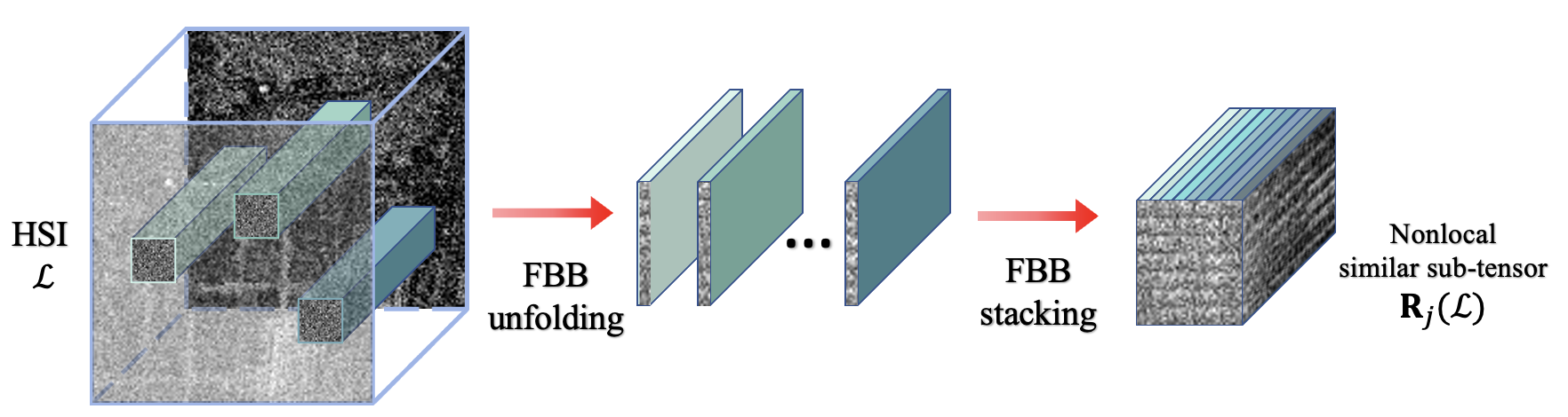
Figure 2: The procedure of block matching.

To be precise, we present the formulations for the $j$-th nonlocal similar sub-tensor extraction operator $\mathbf{R}_{j}$ and then for the nonlocal similar tensor extraction operator $\mathbf{R}$. We define $U_{i}^{(l)}\in\mathbb{R}^{r\times I_{i}}$ be a binary matrix such that $\mathcal{L}\times_{1}U_{1}^{(l)}\times_{2}U_{2}^{(l)}$ is exactly the $l$-th FBB of $\mathcal{L}$. And we define $B_{l}$ as the Casorati matrix (a matrix whose columns are vectorized bands of the HSI) of the $l$-th FBB as follows

$$B_{l}:=\operatorname{reshape}(\mathcal{L}\times_{1}U_{1}^{(l)}\times_{2}U_{2}^{(l)},m_{1},m_{3}),$$

where $m_{1}=r^{2}$ and $m_{3}=I_{3}$. Then the extraction operator of the $j$-th nonlocal similar sub-tensor $\mathbf{R}_{j}:\mathbb{R}^{I_{1}\times I_{2}\times I_{3}}\to\mathbb{R}^{m_{1}\times m_{2}\times m_{3}}$ can be defined by

$$\mathbf{R}_{j}(\mathcal{L}):=\operatorname{reshape}([B_{l_{j1}}^{\top},B_{l_{j2}}^{\top},\dots,B_{l_{jm_{2}}}^{\top}]^{\top},m_{1},m_{2},m_{3}),$$

where the indices $l_{j1},l_{j1},\dots,l_{jm_{2}}$ refer to the indices of FBBs that belongs to the $j$-th nonlocal similar group and $j=1,2,\dots,N$. Then the extraction operator of the nonlocal similar tensor $\mathbf{R}:\mathbb{R}^{I_{1}\times I_{2}\times I_{3}}\to\mathbb{R}^{m_{1}\times m_{2}\times m_{3}\times N}$ is a linear map such that $[\mathbf{R}(\mathcal{L})]^{(j)}=\mathbf{R}_{j}(\mathcal{L})$.

Since the Frobenius inner product is invariant to reshaping, we have that for $\mathcal{Y}\in\mathbb{R}^{m_{1}\times m_{2}\times m_{3}}$,

$$\langle\mathcal{Y},\mathbf{R}_{j}(\mathcal{L})\rangle_{F}=\sum_{i=1}^{m_{2}}\langle{Y}_{:i:},B_{l_{ji}}\rangle_{F}=\langle\mathbf{R}^{\top}_{j}(\mathcal{Y}),\mathcal{L}\rangle_{F},$$

where $\mathbf{R}^{\top}_{j}:\mathbb{R}^{m_{1}\times m_{2}\times m_{3}}\to\mathbb{R}^{I_{1}\times I_{2}\times I_{3}}$ is defined by

(24) $$\mathbf{R}^{\top}_{j}(\mathcal{Y}):=\sum_{i=1}^{m_{2}}\operatorname{reshape}(Y_{:i:},r,r,I_{2})\times_{1}(U_{1}^{(l_{ji})})^{\top}\times_{2}(U_{2}^{(l_{ji})})^{\top}.$$

And we further have that

$$\|\mathbf{R}(\mathcal{L})\|^{2}_{F}=\sum_{j=1}^{N}\|\mathbf{R}_{j}(\mathcal{L})\|_{F}^{2}=\sum_{j=1}^{N}\langle\mathcal{L},\mathbf{R}_{j}^{\top}\mathbf{R}_{j}(\mathcal{L})\rangle_{F}=\|\sqrt{\mathcal{W}_{\mathbf{R}}}\odot\mathcal{L}\|_{F}^{2},$$

where $\odot$ represents the pointwise multiplication, and each entry of $\mathcal{W}_{\mathbf{R}}\in\mathbb{R}^{I_{1}\times I_{2}\times I_{3}}$ represents the number of nonlocal similar groups to which the corresponding pixel belongs. Since we assume that each pixel belongs to at least one nonlocal similar group, we have $\mathcal{W}_{\mathbf{R}}\in\mathbb{R}^{I_{1}\times I_{2}\times I_{3}}_{++}$.

Second, we impose the tensor low-rankness on the nonlocal similar tensor. In the nonlocal sub-tensor $\mathbf{R}_{j}(\mathcal{L})$ that we construct, the first dimension indicates the spatial information, the second dimension reveals the nonlocal self-similarity, and the third dimension reflects the spectral correlation. We adopt the independent 3-D HOSVD to obtain a low-rank approximation of $\mathbf{R}(\mathcal{L})$, that is,

$$\mathbf{R}(\mathcal{L})\approx\mathcal{[}\mathcal{G}]\times_{1}[{X}_{1}]\times_{2}[{X}_{2}]\times_{3}[{X}_{3}],$$

where $[\mathcal{G}]\in\mathbb{R}^{n_{1}\times n_{2}\times n_{3}\times N}$ denotes independent core tensors, and $[{X}_{i}]\in\mathbb{R}^{m_{i}\times n_{i}\times N}$ denotes the $i$-th factor matrices such that $[{X}_{i}]^{\top}[{X}_{i}]=[\mathbf{I}_{n_{i}}]$.

To further boost the low-rankness of $\mathbf{R}(\mathcal{L})$, we propose a sparsity-enhanced nonlocal low-rank tensor regularization term as follows

(25) $$\frac{1}{2}\|\mathcal{[}\mathcal{G}]\times_{1}[{X}_{1}]\times_{2}[{X}_{2}]\times_{3}[{X}_{3}]-\mathbf{R}(\mathcal{L})\|^{2}_{F}+\|[\mathcal{G}]\|_{1,w},$$

where $\|[\mathcal{G}]\|_{1,w}$ is given in (3) with $w\in\mathbb{R}^{N}_{++}$. In particular, the first term of (25) measures the closeness between $\mathbf{R}(\mathcal{L})$ and the approximated low-rank tensor, and the second term measures the sparsity of the independent core tensors $[\mathcal{G}]$. Using the proximal operator of the $\ell_{1}$ norm, the proximal operator of $\|\cdot\|_{1,w}$ can be computed component-wisely by the soft thresholding operator as follows

$$\left(\operatorname{prox}_{\|\cdot\|_{1,w}}([\mathcal{G}])\right)_{i_{1}i_{2}i_{3}}^{(j)} =\operatorname{prox}_{w_{j}|\cdot|}\left([\mathcal{G}]^{(j)}_{i_{1}i_{2}i_{3}}\right)$$

$$=\operatorname{sign}\left([\mathcal{G}]^{(j)}_{i_{1}i_{2}i_{3}}\right)\max\left(\left|[\mathcal{G}]^{(j)}_{i_{1}i_{2}i_{3}}\right|-w_{j},0\right).$$

5.2 Tensor $\ell_{2,p}$ norm for group sparsity

The matrix $\ell_{2,p}$ norm is a nonconvex and nonsmooth function. And it has been applied to image processing [20], machine learning [23, 11], feature selection [19, 31], multi-view classification [33], etc. To measure the linear structural sparsity of the sparse noise tensor $\mathcal{S}$, we extend the matrix $\ell_{2,p}$ norm for group sparsity to its tensor form. As the stripes and dead lines often align the first dimension, we define the tensor $\ell_{2,p}$ $(0<p<1)$ norm in the form of (2), which is exactly the matrix $\ell_{2,p}$ norm of the unfolding matrix along the first dimension.

In the following, we summarize some results for solving the tensor $\ell_{2,p}$ norm minimization problem

(26) $$\min_{\mathcal{S}}\mu\|\mathcal{S}\|^{p}_{2,p}+\frac{1}{2}\|\mathcal{S}-\widetilde{\mathcal{S}}\|^{2}_{F},$$

where $\widetilde{\mathcal{S}}\in\mathbb{R}^{I_{1}\times I_{2}\times I_{3}}$ is a given tensor and parameter $\mu>0$. Since $\|\cdot\|^{p}_{2,p}$ and $\|\cdot\|^{2}_{F}$ are both group-separable, solving problem (26) for $\mathcal{S}$ is equivalent to solving the following subproblem for each $(i_{2},i_{3})$-th vector of $\mathcal{S}$ along the first dimension

(27) $$\min_{s}\mu\|s\|^{p}_{2}+\frac{1}{2}\|s-\tilde{s}\|^{2}_{2},$$

where $s\in\mathbb{R}^{I_{1}}$ and $\tilde{s}\in\mathbb{R}^{I_{1}}$, for simplicity, represent $s_{:i_{2}i_{3}}$ and $\tilde{s}_{:i_{2}i_{3}}$, respectively, and $\|s\|^{p}_{2}=(s_{1}^{2}+s_{2}^{2}+\cdots+s_{I_{1}}^{2})^{\frac{p}{2}}$. It follows from the triangle inequality that the objective function of (27) satisfies the following inequality for any $s\in\mathbb{R}^{I_{1}}$

(28) $$\mu\|s\|^{p}_{2}+\frac{1}{2}\|s-\tilde{s}\|^{2}_{2}\geq\mu\|s\|^{p}_{2}+\frac{1}{2}(\|s\|_{2}-\|\tilde{s}\|_{2})^{2}.$$

And the equality holds if and only if $s=t\tilde{s}$ for some $t\geq 0$ or $\tilde{s}=0$. Observe that the right-hand side of the inequality is only related to $\|s\|_{2}$ and $\|\tilde{s}\|_{2}$. If $\tilde{s}=0$, the solution of problem (27) is $s=0$. If $\tilde{s}\neq 0$, we can view $s$ as $s=t\|\tilde{s}\|_{2}v$ with $t\geq 0$ being a scalar and $v\in\mathbb{R}^{I_{1}}$ being a unit vector. When we restrict the minimization problem (27) by $\|s\|_{2}=t\|\tilde{s}\|_{2}$ with a fixed $t$, according to (28), the solution of the restricted problem of (27) is obtained only when $v=\frac{\tilde{s}}{\|\tilde{s}\|_{2}}$. Hence, if $\tilde{s}\neq 0$, the solution of (27) is $s=t\tilde{s}$, where $t$ is a minimizer of the following problem

(29) $$\min_{t\in[0,\infty)}\nu t^{p}+\frac{1}{2}(t-1)^{2},$$

with $\nu=\mu\|\tilde{s}\|_{2}^{p-2}$. That is, it only requires to solve a one-dimensional problem (29) for computing the solutions of problem (27).

Next, we show a lemma and a solver for computing solutions of problem (27). Let $g(t)=\nu|t|^{p}+\frac{1}{2}(t-1)^{2}$. Note that $g(t)>g(|t|)$ for $\forall t<0$ and $g(t)>g(1)$ for $\forall t>1$. Then problem (29) can be relaxed to an unconstrained problem with $g$ being the objective function, which can be solved using Theorem 1 in [25]. Also, problem (29) can be reduced to a box constrained problem with constraint $t\in[0,1]$, which can be solved using Lemma 4.1 in [21]. We summarize the results for  (29) in the following lemma.

Lemma 5.1.

Let $p\in(0,1)$ and $\nu>0$. Let

$$\nu_{0}:=\frac{[2(1-p)]^{1-p}}{(2-p)^{2-p}},\quad\text{ and }\quad\tau(\nu):=[2\nu(1-p)]^{\frac{1}{2-p}}.$$

Then the set of optimal solutions of problem (29), denoted as $\Omega^{*}(\nu)$, is given by

$$\Omega^{*}(\nu)=\begin{cases}\{0\},\quad&\mbox{if }\nu>\nu_{0};\\ \{0,\tau(\nu_{0})\},\quad&\mbox{if }\nu=\nu_{0};\\ \{t^{*}\},\quad&\mbox{if }0<\nu<\nu_{0},\end{cases}$$

where $t^{*}\in(\tau(\nu),1)$ is the unique solution of the equation

(30) $$\nu pt^{p-1}+t-1=0$$

with $t\in(\tau(\nu),\infty)$.

According to Lemma 5.1, when $\nu=\nu_{0}$, there are two minimizers for problem (29). For simplicity, we will choose $0$ in this case. When $\nu\in(0,\nu_{0})$, the minimizer of problem (29) is unique and can obtained by solving (30). If $p$ is chosen as, for example, $p=1/2$, (30) has a closed-form root. Otherwise, we estimate the unique root $t^{*}$ by Newton’s method with an initial value of $t_{0}=(\tau(\nu)+1)/2$. Altogether, we summarize a proximal operator of the tensor $\ell_{2,p}$ norm in the following theorem.

Theorem 5.2.

Let $p\in(0,1)$ and $\mu>0$. Define the operator $\Gamma_{\mu}:\mathbb{R}\to\mathbb{R}$ by

$$\Gamma_{\mu}(\beta):=\begin{cases}0,\quad&\text{if }\beta\leq\frac{\beta_{0}(2-p)}{2(1-p)};\\ t^{*},\quad&\text{otherwise},\end{cases}$$

where $\beta_{0}=[2\mu(1-p)]^{\frac{1}{2-p}}$, and $t^{*}\in\left[\beta_{0}\beta,1\right)$ is the unique solution of

$$\mu\beta^{p-2}pt^{p-1}+t-1=0,\quad t\in\left[\beta_{0}\beta,\infty\right).$$

Then a solution of the proximal operator of the tensor $\ell_{2,p}$ norm at $\widetilde{\mathcal{S}}\in\mathbb{R}^{I_{1}\times I_{2}\times I_{3}}$ can be computed by

$$\Gamma_{\mu}(\|\tilde{s}_{:i_{2}i_{3}}\|_{2})\tilde{s}_{:i_{2}i_{3}}\in\operatorname{prox}_{\mu\|\cdot\|_{2}^{p}}(\tilde{s}_{:i_{2}i_{3}})=\left(\operatorname{prox}_{\mu\|\cdot\|_{2,p}^{p}}(\widetilde{\mathcal{S}})\right)_{:i_{2}i_{3}},$$

for $i_{2}=1,2,\dots,I_{2}$, $i_{3}=1,2,\dots,I_{3}$.

By applying Theorem 5.2, the update of $\mathcal{S}$ given in (7) can be efficiently computed. In particular, we calculate the $(i_{2},i_{3})$-th mode-$1$ fiber of $\mathcal{S}^{k+1}$ by

$$s_{:i_{2}i_{3}}^{k+1}=\Gamma_{\mu}\left(\left\|\sqrt{w_{:i_{2}i_{3}}}\odot\tilde{s}^{k}_{:i_{2}i_{3}}\right\|_{2}\right)\tilde{s}^{k}_{:i_{2}i_{3}},$$

where $\tilde{\mathcal{S}}^{k}=\mathcal{S}^{k}-\tilde{\alpha}_{\mathcal{S}}\left(\mathcal{S}^{k}+\mathcal{L}^{k}-\mathcal{D}\right)$, and $\tilde{s}^{k}_{:i_{2}i_{3}}$ and $\sqrt{w_{:i_{2}i_{3}}}$ are the $(i_{2},i_{3})$-th mode-$1$ fibers of $\tilde{\mathcal{S}}^{k}$ and $\sqrt{\mathcal{W}_{\mathbf{R}}}$, respectively.

6 Experimental Results

In this section, we conduct numerical experiments for removing mixed noise in HSIs. We compare the proposed methods with five methods, which are BM4D [24] for removing Gaussian noise, and LRTD [8], SNLRSF [5], LRTFL0 [36] and QRNN3D [34] for removing mixed noise. All numerical experiments are implemented in Matlab R2018a and executed on a personal desktop (Intel Core i7 9750H at 2.60 GHz with 16 GB RAM).

6.1 Simulated data experiments

In this subsection, the proposed method and the competing methods are tested on simulated data. The test images are subimages of size $128\times 128\times 128$ randomly obtained from the Washington DC Mall $(1280\times 307\times 191)$ and the Xiong-An $(256\times 256\times 256)$. As shown in Fig. 3, the Washington DC Mall is obtained from an urban area, where buildings are relatively dense; the Xiong-An is obtained from a hilly area, with mountains and shrubs.

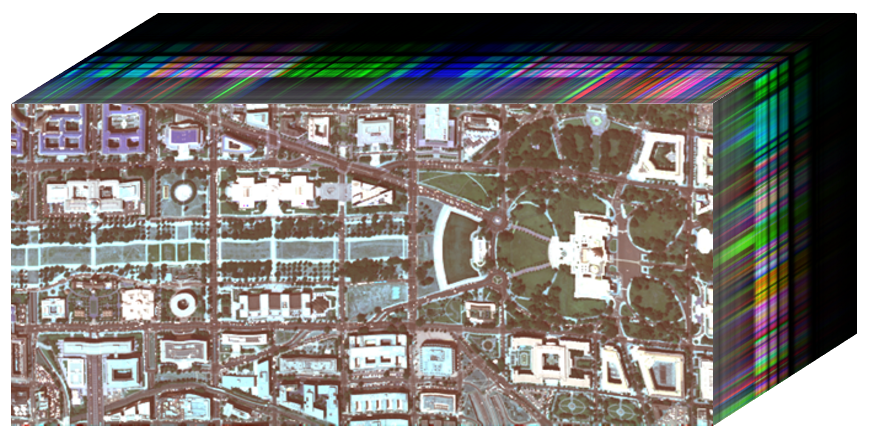
(a) Washington DC Mall

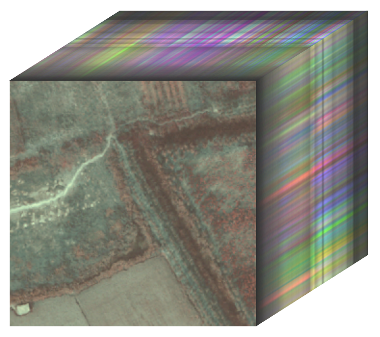
(b) Xiong-An

Figure 3: Original HSIs of two datasets. (a) Part of Washington DC Mall dataset (R:17, G:36, B:46); (b) Xiong-An dataset (R:71, G:110, B:120).

To simulate the noisy HSI data, Gaussian noise, stripes, or dead lines are added to the normalized clean HSI data under the following cases:

• Case 1: Gaussian noise with a mean of zero and a standard deviation of $0.1$ is added to all the bands. And then all the bands are selected and stripes with a density of $30\%$ and a standard deviation of $0.2$ are added to each band.

• Case 2: Gaussian noise with a mean of zero and a standard deviation of $0.1$ is added to all the bands. And then $11-40$, $71-100$, $121-128$ bands are selected and stripes with a density of $20\%$ and a standard deviation of $0.2$ are added to each band.

• Case 3: Gaussian noise with a mean of zero and a standard deviation of $0.2$ is added to all the bands. And then $25\%$ of the bands are randomly selected and dead lines with a density of $5\%$ are added to each band.

For comparing the quality of the restored images, four evaluation metrics are employed, which are the mean peak signal-to-noise ratio (MPSNR), the mean structural similarity index (MSSIM), the mean feature similarity index (MFSIM), and the erreur relative globale adimensionnelle de synthese (ERGAS). Let $\mathcal{X}^{*}$ denote the restored HSI and $\hat{\mathcal{X}}$ denote the clean HSI. Then ${X^{*}_{::i}}$ and $\hat{X}_{::i}$ denote the $i$-th band of the restored HSI and clean HSI, respectively. The MPSNR value is defined as

$$\mathrm{MPSNR}=\frac{1}{I_{3}}\sum^{I_{3}}_{i=1}10\log_{10}\left(\frac{\max^{2}(X^{*}_{::i})}{\mathrm{mse}(X^{*}_{::i},\hat{X}_{::i})}\right),$$

which is the average PSNR value across the bands. Similarly, MSSIM and MFSIM values are defined as

$$\mathrm{MSSIM}=\frac{1}{I_{3}}\sum^{I_{3}}_{i=1}\mathrm{SSIM}(X^{*}_{::i},\hat{X}_{::i})\quad\mbox{ and }\quad\mathrm{MFSIM}=\frac{1}{I_{3}}\sum^{I_{3}}_{i=1}\mathrm{FSIM}(X^{*}_{::i},\hat{X}_{::i}),$$

where SSIM is given in [47] and FSIM is given in [44]. The ERGAS are defined as

$$\mathrm{ERGAS}=100\sqrt{\frac{1}{I_{3}}\sum^{I_{3}}_{i=1}\frac{\mathrm{mse}(X^{*}_{::i},\hat{X}_{::i})}{\mathrm{mean}(X^{*}_{::i})}}.$$

In addition, better denoising results are indicated by larger MPSNR, MSSIM, and MFISM values, as well as smaller ERGAS value.

The numerical results of simulated data experiments for case 1, case 2, and case 3 are presented in Tables 1 and 2 for Washington DC Mall and Xiong-An datasets, respectively. Numerical results in bold font indicate the best performance of the indicator in the current case. It can be observed from Tables 1 and 2 that the proposed NLTL2p method outperforms other methods almost in terms of all the evaluation metrics. For example, in case 1 of Xiong-An dataset, the MPSNR value of the HSI restored by the NLTL2p method is 1.84 dB larger than the MPSNR value of the second best method, that is, the LRTFL0 method.

Table 1: Numerical results tested on Washington DC Mall dataset

Case	Index	Noisy	NLTL2p	LRTFL0	SNLRSF	LRTD	BM4D	QRNN3D
1	MPSNR	14.90	30.49	30.29	25.92	26.47	16.35	25.27
	MSSIM	0.324	0.928	0.923	0.795	0.817	0.399	0.794
	MFSIM	0.653	0.949	0.957	0.902	0.907	0.724	0.885
	ERGAS	518.02	92.41	92.45	151.04	138.47	438.24	159.34
2	MPSNR	16.72	32.14	30.46	31.45	27.82	22.72	26.97
	MSSIM	0.428	0.939	0.920	0.912	0.854	0.639	0.844
	MFSIM	0.703	0.962	0.933	0.950	0.921	0.817	0.916
	ERGAS	419.52	91.63	78.65	83.10	105.07	330.58	119.73
3	MPSNR	13.90	30.66	29.83	28.01	25.44	20.80	25.62
	MSSIM	0.390	0.943	0.924	0.895	0.801	0.762	0.842
	MFSIM	0.680	0.963	0.929	0.943	0.897	0.879	0.913
	ERGAS	610.91	90.35	93.19	141.32	148.89	449.91	147.69

Table 2: Numerical results tested on Xiong-An dataset

Case	Index	Noisy	NLTL2p	LRTFL0	SNLRSF	LRTD	BM4D	QRNN3D
1	MPSNR	14.49	33.57	31.73	26.26	30.02	15.88	26.53
	MSSIM	0.102	0.864	0.810	0.562	0.710	0.151	0.633
	MFSIM	0.482	0.928	0.915	0.829	0.883	0.575	0.852
	ERGAS	382.96	43.96	55.28	112.07	66.10	328.21	97.50
2	MPSNR	17.19	33.43	33.21	30.25	30.71	24.29	28.27
	MSSIM	0.159	0.875	0.837	0.719	0.730	0.468	0.694
	MFSIM	0.562	0.928	0.924	0.885	0.894	0.722	0.880
	ERGAS	306.56	45.12	48.82	80.07	60.80	234.71	82.38
3	MPSNR	13.90	31.48	30.89	28.39	27.96	21.30	26.13
	MSSIM	0.238	0.912	0.858	0.828	0.765	0.692	0.755
	MFSIM	0.634	0.954	0.897	0.924	0.881	0.831	0.900
	ERGAS	435.95	58.47	56.64	103.41	83.80	321.25	101.38

For visual quality comparison, the HSIs restored by different methods are presented in Fig. 4-7, with a subregion marked by a white box and enlarged in a white box. The NLTL2p method achieves state-of-the-art performance for HSI denoising and destriping, while the competing methods seem to fail to remove noises or to restore HSIs with high quality. For example, for removing mixed noise, the BM4D method fails to remove stripes even if the HSI only contains few stripes as shown in Fig. 5(5(g)); the SNLRSF and QRNN3D methods fail to remove the stripes and dead lines, when the noise level is high, for example, in Fig. 4(4(e))(4(h)) and Fig. 6(6(e))(7(h)). Also, regarding the quality of the restoration, the HSIs restored by the LRTD method look a little noisy and blurry, for example, in Fig. 4(4(f)); the HSIs restored by the LRTFL0 method looks oversmooth with some details missing, for example, in Fig. 6(6(d)) and Fig. 7(7(d)).

(a) Noisy image

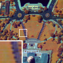
(b) Ground truth

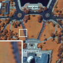
(c) NLTL2p (ours)

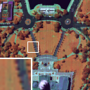
(d) LRTFL0

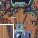
(e) SNLRSF

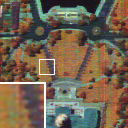
(f) LRTD

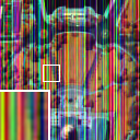
(g) BM4D

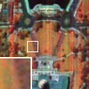
(h) QRNN3D

Figure 4: Comparison of HSIs (R:3, G:43, B:75) restored by different methods from Washington DC Mall in case 1. The PSNR value for each restored HSI: (a) Noisy image (14.90 dB); (c) NLTL2p (ours) (30.49 dB); (d) LRTFL0 (30.29 dB); (e) SNLRSF (25.92 dB); (f) LRTD (26.47 dB); (g) BM4D (16.35 dB); (h) QRNN3D (25.27 dB).

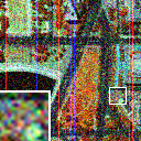
(a) Noisy image

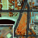
(b) Ground truth

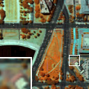
(c) NLTL2p (ours)

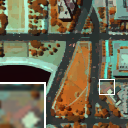
(d) LRTFL0

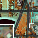
(e) SNLRSF

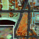
(f) LRTD

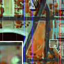
(g) BM4D

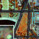
(h) QRNN3D

Figure 5: Comparison of HSIs (R:16, G:70, B:100) restored by different methods from Washington DC Mall in case 3. The PSNR value for each restored HSI: (a) Noisy image (13.90 dB); (c) NLTL2p (ours) (30.66 dB); (d) LRTFL0 (29.83 dB); (e) SNLRSF (28.01 dB); (f) LRTD (25.44 dB); (g) BM4D (20.80 dB); (h) QRNN3D (25.62 dB).

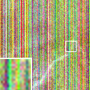
(a) Noisy image

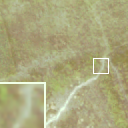
(b) Ground truth

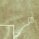
(c) NLTL2p (ours)

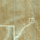
(d) LRTFL0

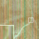
(e) SNLRSF

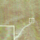
(f) LRTD

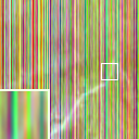
(g) BM4D

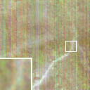
(h) QRNN3D

Figure 6: Comparison of HSIs (R:30, G:55, B:115) restored by different methods from Xiong-An in case 1. The PSNR value for each restored HSI: (a) Noisy image (14.49 dB); (c) NLTL2p (ours) (33.57 dB); (d) LRTFL0 (31.73 dB); (e) SNLRSF (26.26 dB); (f) LRTD (30.02 dB); (g) BM4D (15.88 dB); (h) QRNN3D (26.53 dB).

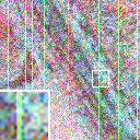
(a) Noisy image

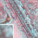
(b) Ground truth

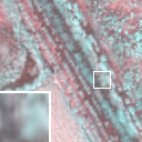
(c) NLTL2p (ours)

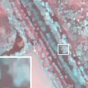
(d) LRTFL0

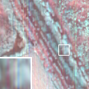
(e) SNLRSF

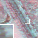
(f) LRTD

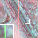
(g) BM4D

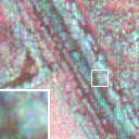
(h) QRNN3D

Figure 7: Comparison of HSIs (R:38, G:87, B:120) restored by different methods from Xiong-An in case 3. The PSNR value for each restored HSI: (a) Noisy image (13.90 dB); (c) NLTL2p (ours) (31.48 dB); (d) LRTFL0 (30.89 dB); (e) SNLRSF (28.39 dB); (f) LRTD (27.96 dB); (g) BM4D (21.30 dB); (h) QRNN3D (26.13 dB).

6.2 Real data experiments

In this subsection, we test the proposed method and the competing methods on two real HSI datasets containing mixed noise. The test images are subimages of size $128\times 128\times 128$ randomly obtained from the HYDICE Urban $(307\times 307\times 210)$ and EO-1 Hyperion $(400\times 200\times 166)$, which are shown in Fig. 8. A selected band of the HSI restored by each method is presented in Fig. 9 and Fig. 10 for HYDICE Urban dataset and EO-1 Hyperion dataset, respectively. It can be observed that the proposed NLTL2p method can remove the stripes while preserving the image details. However, the LRTFL0, LRTD, BM4D and QRNN3D methods are unable to eliminate the stripes when the band is contaminated by heavy mixed noise as shown in Fig. 9; and the SNLRSF, LRTD, BM4D and QRNN3D methods remove not only the noise but also some structural details of the HSI as shown in Fig. 10.

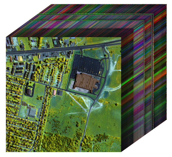
(a) HYDICE Urban

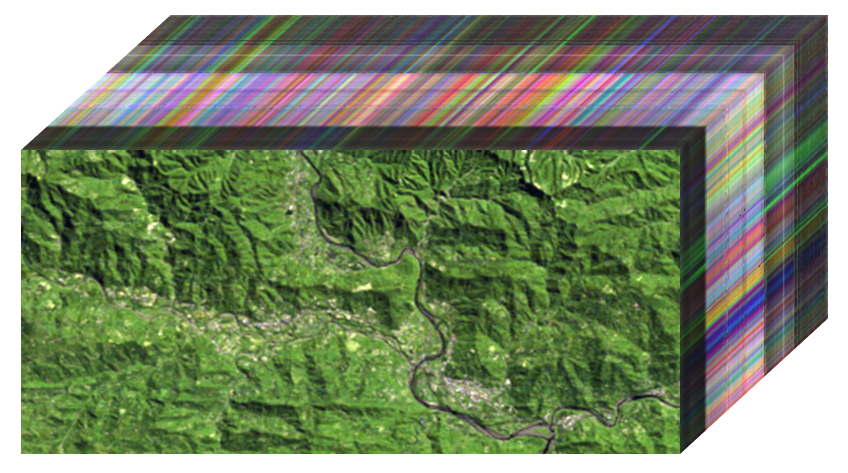
(b) EO-1 Hyperion

Figure 8: Real HSIs of two datasets. (a) HYDICE Urban dataset (R:61, G:98, B:170); (b) EO-1 Hyperion dataset (R:101, G:114, B:160).

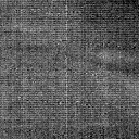
(a) Noisy image

(b) NLTL2p (ours)

(c) LRTFL0

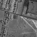
(d) SNLRSF

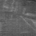
(e) LRTD

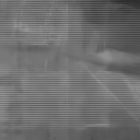
(f) BM4D

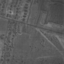
(g) QRNN3D

Figure 9: Comparison of the 25-th band of the HSI restored by different methods from HYDICE Urban.

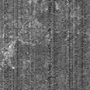
(a) Noisy image

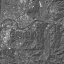
(b) NLTL2p (ours)

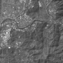
(c) LRTFL0

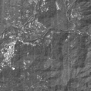
(d) SNLRSF

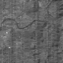
(e) LRTD

(f) BM4D

(g) QRNN3D

Figure 10: Comparison of the 128-th band of the HSI restored by different methods from EO-1 Hyperion.

6.3 Parameter analysis

For the proposed NLTL2p method, we set block matching with $(m_{1},m_{2},m_{3})=(25,128,128)$ and $(n_{1},n_{2},n_{3})=(25,2,32)$; we set model parameters $\delta\in[0.4,0.6]$, $w_{j}=10^{2}$, $p=0.1$, and $\gamma\in[100,200]$; and we set algorithm parameters $\alpha_{\mathcal{S}}=\alpha_{X}=\alpha_{\mathcal{G}}=0.001$. In practice, to accelerate the algorithm, we update $\mathbf{R}$ via block matching on FBBs for several iterations in the beginning and then fix it for the remaining iterations. Also, we perform the updates of $[X_{i}]$ and $[\mathcal{G}]$ three times as inner iterations for boosting the nonlocal low-rank regularization process. Note that these practical strategies will not affect the convergence of the algorithm. And Algorithm 1 stops if $\|\mathcal{L}^{k+1}-\mathcal{L}^{k}\|_{F}/\|\mathcal{L}^{k}\|_{F}\leq 0.01$.

To further analyze the parameters in the proposed model, we use case 3 of Washington DC Mall for testing. First, we test the proposed NLTL2p method with different values of $\delta$ and $\gamma$. The plot of MPSNR values vs parameters is presented in Fig. 11(11(a)). When the value of $\gamma$ is fixed, the change of MPSNR over $\delta$ is not obvious. When the value of $\delta$ is fixed, the MPSNR value is larger than 29 dB if $\gamma\in[100,200]$.

Second, we test the proposed NLTL2p method with different values of $p$ and $\gamma$ and plot the MPSNR values vs parameters in Fig. 11(11(b)). When the value of $\gamma$ is fixed, the MPSNR value is larger if $p$ is smaller. When the value of $p$ is less than $0.5$, the best MPSNR value is achieved if $\gamma\in[100,200]$.

In summary, the proposed method is not very sensitive to $\delta$ and can achieve great performance when $\gamma$ is between $100$ and $200$, and $p$ is close to $0$.

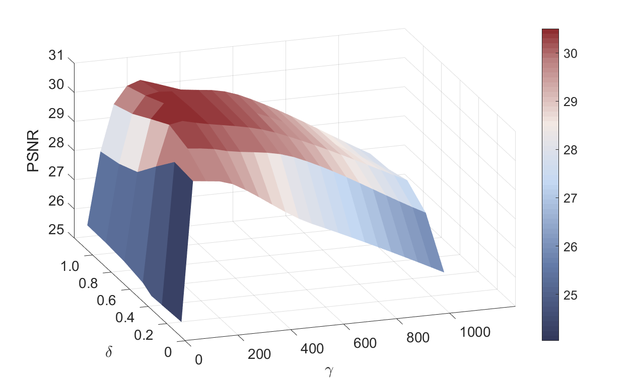
(a) Plot on $\delta$ and $\gamma$.

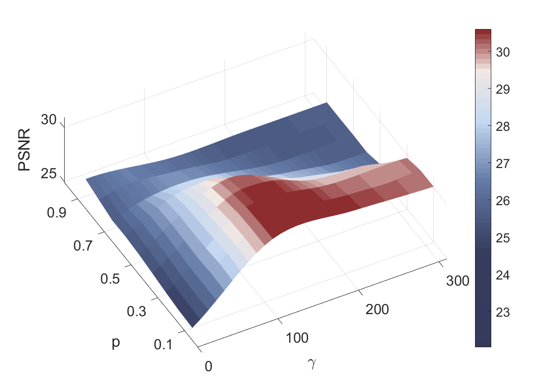
(b) Plot on $p$ and $\gamma$

Figure 11: Plots of the MPSNR values obtained by our proposed method vs several parameters.

7 Conclusions

In this paper, we propose an HSI denoising and destriping method, which has an optimization model given in (1) and an iterative algorithm described in Algorithm 1. The optimization model consists of a data fidelity term, a sparsity-enhanced nonlocal low-rank tensor regularization term for denoising, and a $\ell_{2,p}$ norm for destriping. The iterative algorithm is proposed using a proximal version of BCD algorithms, which has convergence guarantees. The numerical experiments tested on simulated and real HSIs also show the effectiveness of our proposed method in removing Gaussian noise, stripes, and deadlines.

References

• [1] P. A. Absil, R. Mahony, and R. Sepulchre, Optimization on Matrix Manifolds, Princeton University Press, 2008.
• [2] P. A. Absil and J. Malick, Projection-like retractions on matrix manifolds, SIAM J. Optim., 22 (2012), pp. 135–158.
• [3] J. Bolte, S. Sabach, and M. Teboulle, Proximal alternating linearized minimization for nonconvex and nonsmooth problems, Math. Program., 146 (2014), pp. 459–494.
• [4] J. Bradbury, S. Merity, C. Xiong, and R. Socher, Quasi-recurrent neural networks, arXiv preprint arXiv:1611.01576, (2016).
• [5] C. Cao, J. Yu, C. Zhou, K. Hu, F. Xiao, and X. Gao, Hyperspectral image denoising via subspace-based nonlocal low-rank and sparse factorization, IEEE J. Sel. Top. Appl. Earth Obs. Remote Sens., 12 (2019), pp. 973–988.
• [6] C.-I. Chang, Hyperspectral imaging: techniques for spectral detection and classification, vol. 1, Springer Science & Business Media, 2003.
• [7] J. Chen and Y. Saad, On the tensor SVD and the optimal low rank orthogonal approximation of tensors, SIAM J. Matrix Anal. Appl., 30 (2009), pp. 1709–1734.
• [8] Y. Chen, T.-Z. Huang, and X.-L. Zhao, Destriping of multispectral remote sensing image using low-rank tensor decomposition, IEEE J. Sel. Top. Appl. Earth Obs. Remote Sens., 11 (2018), pp. 4950–4967.
• [9] K. Dabov, A. Foi, V. Katkovnik, and K. Egiazarian, Image denoising by sparse 3-D transform-domain collaborative filtering, IEEE Trans. Image Process., 16 (2007), pp. 2080–2095.
• [10] J. H. de Morais Goulart and G. Favier, Low-rank tensor recovery using sequentially optimal modal projections in iterative hard thresholding (SeMPIHT), SIAM J. Sci. Comput., 39 (2017), pp. A860–A889.
• [11] Y. Ding, W. He, J. Tang, Q. Zou, and F. Guo, Laplacian regularized sparse representation based classifier for identifying DNA N4-methylcytosine sites via $l_{2,1/2}$-matrix norm, IEEE ACM Trans. Comput. Bi., 20 (2021), pp. 500–511.
• [12] M. Elad and M. Aharon, Image denoising via sparse and redundant representations over learned dictionaries, IEEE Trans. Image Process., 15 (2006), pp. 3736–3745.
• [13] B. Gao, X. Liu, X. Chen, and Y.-X. Yuan, A new first-order algorithmic framework for optimization problems with orthogonality constraints, SIAM J. Optim., 28 (2018), pp. 302–332.
• [14] K. Gao and Z.-H. Huang, Tensor robust principal component analysis via tensor fibered rank and minimization, SIAM J. Imaging Sci., 16 (2023), pp. 423–460.
• [15] H. Grahn and P. Geladi, Techniques and applications of hyperspectral image analysis, John Wiley & Sons, 2007.
• [16] J. Guo, Y. Guo, Q. Jin, M. Kwok-Po Ng, and S. Wang, Gaussian patch mixture model guided low-rank covariance matrix minimization for image denoising, SIAM J. Imaging Sci., 15 (2022), pp. 1601–1622.
• [17] N. J. Higham, Matrix nearness problems and applications, Applications of Matrix Theory, 22 (1989).
• [18] B.-Z. Li, X.-L. Zhao, X. Zhang, T.-Y. Ji, X. Chen, and M. K. Ng, A learnable group-tube transform induced tensor nuclear norm and its application for tensor completion, SIAM J. Imaging Sci., 16 (2023), pp. 1370–1397.
• [19] Z. Li, F. Nie, J. Bian, D. Wu, and X. Li, Sparse PCA via $\ell_{2,p}$-norm regularization for unsupervised feature selection, IEEE Trans. Pattern Anal., 45 (2021), pp. 5322–5328.
• [20] Z. Li, J. Tang, and X. He, Robust structured nonnegative matrix factorization for image representation, IEEE Trans. Neur. Net. Lear., 29 (2017), pp. 1947–1960.
• [21] T. Liu, Z. Lu, X. Chen, and Y.-H. Dai, An exact penalty method for semidefinite-box-constrained low-rank matrix optimization problems, IMA J. Numer. Anal., 40 (2018), pp. 563–586.
• [22] X. Liu, J. Lu, L. Shen, C. Xu, and Y. Xu, Multiplicative noise removal: Nonlocal low-rank model and its proximal alternating reweighted minimization algorithm, SIAM J. Imaging Sci., 13 (2020), pp. 1595–1629.
• [23] X. Ma, Q. Ye, and H. Yan, L2p-norm distance twin support vector machine, IEEE Access, 5 (2017), pp. 23473–23483.
• [24] M. Maggioni, V. Katkovnik, K. Egiazarian, and A. Foi, Nonlocal transform-domain filter for volumetric data denoising and reconstruction, IEEE Trans. Image Process., 22 (2012), pp. 119–133.
• [25] G. Marjanovic and V. Solo, On $l_{q}$ optimization and matrix completion, IEEE Trans. Signal Process., 60 (2012), pp. 5714–5724.
• [26] J. Pan, M. K. Ng, Y. Liu, X. Zhang, and H. Yan, Orthogonal nonnegative Tucker decomposition, SIAM J. Sci. Comput., 43 (2021), pp. B55–B81.
• [27] C. Prévost, R. A. Borsoi, K. Usevich, D. Brie, J. C. Bermudez, and C. Richard, Hyperspectral super-resolution accounting for spectral variability: Coupled tensor ll1-based recovery and blind unmixing of the unknown super-resolution image, SIAM J. Imaging Sci., 15 (2022), pp. 110–138.
• [28] A. Rajwade, D. Kittle, T.-H. Tsai, D. Brady, and L. Carin, Coded hyperspectral imaging and blind compressive sensing, SIAM J. Imaging Sci., 6 (2013), pp. 782–812.
• [29] Y. Song, E.-H. Djermoune, J. Chen, C. Richard, and D. Brie, Online deconvolution for industrial hyperspectral imaging systems, SIAM J. Imaging Sci., 12 (2019), pp. 54–86.
• [30] H. Sun, M. Liu, K. Zheng, D. Yang, J. Li, and L. Gao, Hyperspectral image denoising via low-rank representation and CNN denoiser, IEEE J. Sel. Top. Appl. Earth Obs. Remote Sens., 15 (2022), pp. 716–728.
• [31] L. Wang and S. Chen, $l\_${$2,p$} matrix norm and its application in feature selection, arXiv preprint arXiv:1303.3987, (2013).
• [32] Y. Wang, J. Peng, Q. Zhao, Y. Leung, X.-L. Zhao, and D. Meng, Hyperspectral image restoration via total variation regularized low-rank tensor decomposition, IEEE J. Sel. Top. Appl. Earth Obs. Remote Sens., 11 (2017), pp. 1227–1243.
• [33] Z. Wang, Q. Lin, Y. Chen, and P. Zhong, Block-based multi-view classification via view-based $l_{2,p}$ sparse representation and adaptive view fusion, Eng. Appl. Artif. Intel., 116 (2022), p. 105337.
• [34] K. Wei, Y. Fu, and H. Huang, 3-D quasi-recurrent neural network for hyperspectral image denoising, IEEE Trans. Neur. Net. Lear., 32 (2020), pp. 363–375.
• [35] Z. Xing, M. Zhou, A. Castrodad, G. Sapiro, and L. Carin, Dictionary learning for noisy and incomplete hyperspectral images, SIAM J. Imaging Sci., 5 (2012), pp. 33–56.
• [36] F. Xiong, J. Zhou, and Y. Qian, Hyperspectral restoration via $l_{0}$ gradient regularized low-rank tensor factorization, IEEE Trans. Geosci. Remote Sens., 57 (2019), pp. 10410–10425.
• [37] Y. Xu and W. Yin, A globally convergent algorithm for nonconvex optimization based on block coordinate update, J. Sci. Comput., 72 (2017), pp. 700–734.
• [38] F. Yang, X. Chen, and L. Chai, Hyperspectral image destriping and denoising using stripe and spectral low-rank matrix recovery and global spatial-spectral total variation, Remote Sens., 13 (2021), p. 827.
• [39] Q. Yu and M. Bai, Generalized nonconvex hyperspectral anomaly detection via background representation learning with dictionary constraint, SIAM J. Imaging Sci., 17 (2024), pp. 917–950.
• [40] Q. Yuan, L. Zhang, and H. Shen, Hyperspectral image denoising employing a spectral–spatial adaptive total variation model, IEEE Trans. Geosci. Remote Sens., 50 (2012), pp. 3660–3677.
• [41] Q. Yuan, Q. Zhang, J. Li, H. Shen, and L. Zhang, Hyperspectral image denoising employing a spatial–spectral deep residual convolutional neural network, IEEE Trans. Geosci. Remote Sens., 57 (2018), pp. 1205–1218.
• [42] H. Zhang, J. Cai, W. He, H. Shen, and L. Zhang, Double low-rank matrix decomposition for hyperspectral image denoising and destriping, IEEE Trans. Geosci. Remote Sens., 60 (2022), pp. 1–19.
• [43] H. Zhang, W. He, L. Zhang, H. Shen, and Q. Yuan, Hyperspectral image restoration using low-rank matrix recovery, IEEE Trans. Geosci. Remote Sens., 52 (2013), pp. 4729–4743.
• [44] L. Zhang, L. Zhang, X. Mou, and D. Zhang, FSIM: A feature similarity index for image quality assessment, IEEE Trans. Image Process., 20 (2011), pp. 2378–2386.
• [45] Y.-Q. Zhao and J. Yang, Hyperspectral image denoising via sparse representation and low-rank constraint, IEEE Trans. Geosci. Remote Sens., 53 (2014), pp. 296–308.
• [46] H. Zheng, Y. Lou, G. Tian, and C. Wang, A scale-invariant relaxation in low-rank tensor recovery with an application to tensor completion, SIAM J. Imaging Sci., 17 (2024), pp. 756–783.
• [47] W. Zhou, B. Alan Conrad, S. Hamid Rahim, and E. P. Simoncelli, Image quality assessment: from error visibility to structural similarity, IEEE Trans. Image Process., 13 (2004), pp. 600–612.