A Fast Dynamic Point Detection Method for LiDAR-Inertial Odometry in Driving Scenarios

Abstract

Existing 3D point-based dynamic point detection and removal methods have a significant time overhead, making them difficult to adapt to LiDAR-inertial odometry systems. This paper proposes a label consistency based dynamic point detection and removal method for handling moving vehicles and pedestrians in autonomous driving scenarios, and embeds the proposed dynamic point detection and removal method into a self-designed LiDAR-inertial odometry system. Experimental results on three public datasets demonstrate that our method can accomplish the dynamic point detection and removal with extremely low computational overhead (i.e., 1$\sim$9ms) in LIO systems, meanwhile achieve comparable preservation rate and rejection rate to state-of-the-art methods and significantly enhance the accuracy of pose estimation. We have released the source code of this work for the development of the community.

I Introduction

In the field of autonomous driving, 3D light detection and ranging (LiDAR) and inertial measurement units (IMUs) are widely used sensors for real-time localization. IMU provides motion priors, ensuring the accuracy and low latency of state estimation. Meanwhile, LiDAR offers geometric constraints for pose solution and accurately perceives the 3D structure of the scene. Consequently, LiDAR-inertial odometry (LIO) [23, 19] has become the predominant framework for real-time state estimation.

Most existing LIO systems are designed based on the assumption of static environment. However, in practical applications, vehicle platforms often travel in dynamic scenes filled with moving vehicles and pedestrians. The point cloud data collected from dynamic objects cannot construct consistent pose constraints as static points, which is detrimental to state estimation. Moreover, the ghost tracks of moving objects can severely affect the visualization of the reconstructed map (as shown in Fig. 1 (a)).

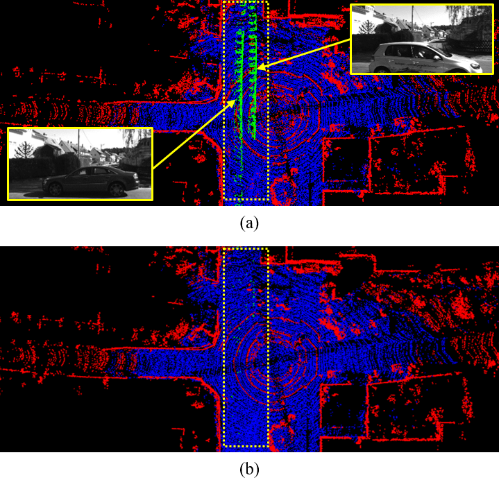
Figure 1: Illustration of (a) the exemplar point cloud map with dynamic points, where green points are ghost tracks of moving vehicles. (b) the static point cloud map, where the dynamic points have been detected and removed by our label consistency-based dynamic point detection and removal method.

To mitigate the interference of dynamic environments on the performance of LIO, several 3D point-based dynamic point detection methods have been successively proposed. They are broadly divided into offline and online categories. The offline methods (e.g., Removert [9], ERASOR [10], DORF [4]) requires a pre-built map to accurately filter out dynamic points, which is clearly unsuitable for LIO as the LIO system does not rely on pre-built prior map. The online methods (e.g., Dynamic Filter [6], Dynablox [13], RH-Map [22]), although theoretically not requiring pre-built maps, need a huge computational cost that makes it difficult to run in real time or barely able to run in real time. This computational overhead also does not meet the requirements of LIO as the LIO system also requires computational resources to complete the basic tasks of state estimation and map update. Generally, a LIO can only allocate a limited amount of computational resources for dynamic point detection and removal. Therefore, ensuring the low computational cost of dynamic object detection methods is very important.

In this paper, we propose a label consistency based dynamic point detection and removal method for handling moving vehicles and pedestrians in autonomous driving scenarios. The method first rapidly separates ground points from the input sweep using [14], and labels them with the “ground point” tag and marks non-ground points with the “non-ground point” tag. Since vehicles and pedestrians are both situated on the ground, there will be inconsistencies in the labels when finding nearest neighbor for points located on vehicles and pedestrians. If a LiDAR point’s own label is “non-ground point”, but most of its nearest neighbor points are “ground points”, it is considered a dynamic point. Dynamic points will not be added to the global map to ensure that the final reconstructed map contains only static points (as shown in Fig. 1 (b)).

The experimental results on semantic-KITTI [1] dataset demonstrate that our dynamic point detection and removal method achieves state-of-the-art preservation rate (PR) and rejection rate (RR), and significantly outperforms online methods, e.g., Dynamic Filter [6] and RH-Map [22] in terms of smaller computational time. The experimental results on the ULHK-CA [17] and UrbanNav [7] datasets indicate that the incorporation of our dynamic point detection and removal method has led to a great improvement in the accuracy of estimated pose, outperforming the current state-of-the-art LIO systems. Compared to other LIO systems, our approach exhibits a significant advantage in terms of computational overhead.

To summarize, the main contributions of this work are three folds: 1) We propose a label consistency based dynamic point detection and removal method, which is capable of detecting and removing dynamic points with a relatively low computational cost; 2) We incorporate the label consistency based dynamic point detection and removal method into a LIO system and enhance the accuracy of estimated pose; 3) We have released the source code of our system to benefit the development of the community.

The rest of this paper is structured as follows. Sec. II reviews the relevant literature. Sec. III provides preliminaries. Secs. IV and V presents system overview and details, followed by experimental evaluation in Sec. VI. Sec. VII concludes the paper.

II Related Work

The 3D point-based dynamic point detection and removal methods can be broadly divided into offline and online categories. The offline methods (e.g., Removert [9], ERASOR [10], DORF [4]) requires a pre-built map to accurately filter out dynamic points. Removert [9] proposed a multiresolution range image-based false prediction reverting algorithm. It first conservatively retained definite static points and iteratively recover more uncertain static points by enlarging the query-to-map association window size, which implicitly compensates the LiDAR motion or registration errors. ERASOR [10] proposed the novel concept called pseudo occupancy to express the occupancy of unit space and then discriminate spaces of varying occupancy. Then, the region-wise ground plane fitting (R-GPF) is adopted to distinguish static points from dynamic points within the candidate bins that potentially contain dynamic points. DORF [4] proposed a novel coarse-to-fine offline framework that exploits global 4D spatial-temporal LiDAR information to achieve clean static point cloud map generation. DORF first conservatively preserved the definite static points leveraging the receding horizon sampling (RHS) mechanism, then gradually recovered more ambiguous static points, guided by the inherent characteristic of dynamic objects in urban environments. The online methods (e.g., Dynamic Filter [6], Dynablox [13], RH-Map [22]) do not require pre-built maps. Dynamic Filter [6] proposed a novel online removal framework for highly dynamic urban environments. The framework consists of the scan-to-map front-end and the map-to-map back-end modules. Both the front-ends and back-ends deeply integrate the visibility-based approach and map-based approach. Dynablox [13] proposed to incrementally estimate high confidence free-space areas by modeling and accounting for sensing, state estimation, and mapping limitations during online robot operation. It can achieve robust moving object detection in complex unstructured environments. RH-Map [22] proposed a novel map construction framework based on 3D region-wise hash map structure, which adopt the two-layer 3D region-wise hash map structure and the region-wise ground plane estimation for dynamic object removal.

In recent years, various LIO systems have been proposed in the robotics community. LIO-SAM [15] firstly formulated LIO odometry as a factor graph, which allows a multitude of relative and absolute measurements, including loop closures, to be incorporated from different sources as factors into the system. In LINs [12], a pioneering integration of 6-axis IMU and 3D LiDAR is accomplished within an error state iterated Kalman filter (ESIKF) framework. This design ensures that the computational demands of the system remain tractable. Drawing from mathematical foundations, Fast-LIO [21] adapts a technique of solving Kalman gain [16], circumventing the need for high-order matrix inversion, thereby significantly alleviating the computational load. Building upon the advancements of Fast-LIO, Fast-LIO2 [20] introduces an innovative ikd-tree algorithm [2]. Compared to the traditional kd-tree, this algorithm offers reduced temporal expenditure in processes such as tree construction, traversal, and element removal. DLIO [3] proposed to preserve a third-order minimum within the realms of state prediction and point distortion calibration, thereby facilitating the acquisition of more precise pose estimation. Semi-Elastic-LIO [25] proposed a semi-elastic optimization-based LiDAR-inertial state estimation method, which imparts sufficient elasticity to the state to allow it be optimized to the correct value. SR-LIO [24] adapt the sweep reconstruction method [26], which segments and reconstructs raw input sweeps from spinning LiDAR to obtain reconstructed sweeps with higher frequency. Consequently, the frequency of estimated pose is also increased. RF-LIO [11] utilized an adaptive multi-resolution range images to first remove dynamic objects, and then match LiDAR sweeps to the map for state estimation. ID-LIO [18] proposed a LiDAR inertial odometry based on indexed point and delayed removal strategy for dynamic scenes, which builds on LIO-SAM. Although RF-LIO and ID-LIO have the ability to perform state estimation in dynamic scenarios, huge computational overhead makes them unable to run stably in real time.

III Preliminary

III-A Coordinate Systems

We denote $(\cdot)^{w}$, $(\cdot)^{l}$ and $(\cdot)^{o}$ as a 3D point in the world coordinate, the LiDAR coordinate and the IMU coordinate respectively. The world coordinate is coinciding with $(\cdot)^{o}$ at the starting position.

We denote the IMU coordinate for taking the $i_{th}$ IMU measurement at time $t_{i}$ as $o_{i}$, then the transformation matrix (i.e., external parameters) from $l_{i}$ to $o_{i}$ is denoted as $\mathbf{T}_{l_{i}}^{o_{i}}\in SE(3)$, where $\mathbf{T}_{l_{i}}^{o_{i}}$ consists of a rotation matrix $\mathbf{R}_{l_{i}}^{o_{i}}\in SO(3)$ and a translation vector $\mathbf{t}_{l_{i}}^{o_{i}}\in\mathbb{R}^{3}$. Typically, it is assumed that the extrinsic parameter matrix $\mathbf{T}_{l_{i}}^{o_{i}}$ has been sufficiently accurately calibrated offline, and thus it is not further optimized in subsequent processes. Consequently, we simplify $\mathbf{T}_{l_{i}}^{o_{i}}$ to $\mathbf{T}_{l}^{o}$.

IV System Overview

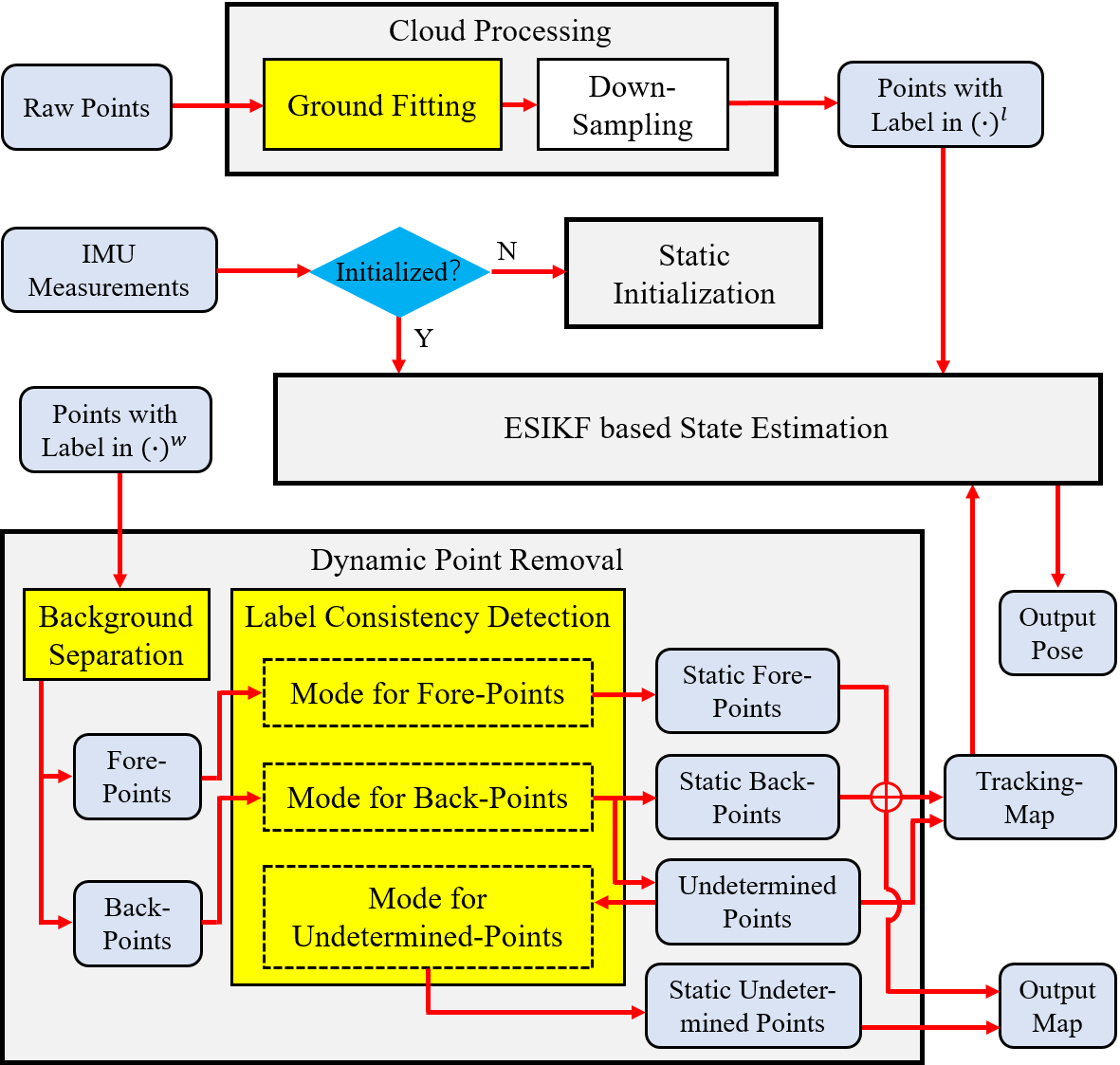
Figure 2: Overview of our Dynamic-LIO which consists of four main modules: cloud processing, static initialization, ESIKF based state estimation and dynamic point removal. The yellow rectangles indicate the operations of our system that are related to dynamic point detection and removal.

Fig. 2 illustrates the framework of our system which consists of four main modules: cloud processing, static initialization, ESIKF based state estimation and dynamic point removal. The cloud processing module segregates ground points from current input point cloud data, and assigns each 3D point with labels indicating “ground point” or “non-ground point”. Subsequently, it performs spatial down sampling to ensure uniform density of current point cloud. The static initialization module utilizes the IMU measurements to estimate some state parameters such as gravitational acceleration, accelerometer bias, gyroscope bias and initial velocity. The ESIKF based state estimation module estimates the state of current sweep, where the execution process is entirely consistent with the state estimation module of SR-LIO [24]. All nearest neighbor query operations during point cloud registration are conducted on the tracking-map. The dynamic point removal module detects dynamic points using a label consistency-based dynamic point detection method and removes them during map updating to ensure that the map contains only static points. The entire system maintains two global maps: the tracking-map and the output-map. The former is utilized for the state estimation, while the latter serves as the final reconstruction outcome. Compared to the tracking-map, the dynamic points in the output-map are filtered more thoroughly. For tracking-map and output-map management, we utilized the Hash voxel map, which is the same as CT-ICP [5]. The implementation details of various parts of white rectangles are exactly the same as our previous work SR-LIO [24], therefore, we omit the introduction of these parts, and only introduce the details of yellow rectangles related to dynamic point detection and removal in Sec. V.

V System Details

V-A Ground Fitting

We utilize the same ground segmentation as LeGO-LOAM [14] to separate ground points from current input sweep with very low computational cost, which is highly valued for LIO systems. The visualization of separating ground points is illustrated in Fig. 3, where the orange points are labeled as “ground points” and the white points are labeled as “non-ground points”.

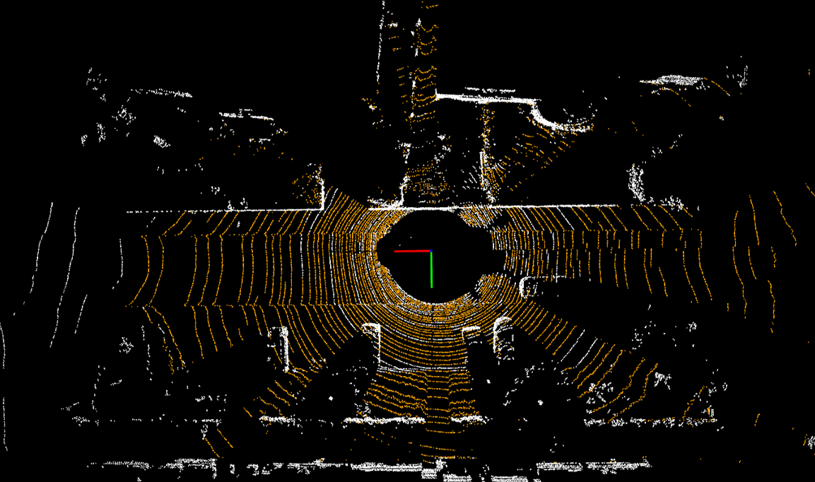
Figure 3: Visualization of separating ground points from current input sweep. The orange points represent ground points and the white points represent non-ground points.

V-B Background Separation

During the execution of label consistency detection, it is necessary to find the nearest neighbor for each point in the current sweep. Points that are close to the vehicle platform can reliably find their nearest neighbors, whereas points that are farther away from the vehicle platform may fail to find their nearest neighbors due to the fact that their locations have not yet been reconstructed. We set a threshold of 30 meters, defining points within 30 meters of the vehicle platform as fore-points and those beyond 30 meters as back-points. For fore-points and back-points, we employ label consistency-based dynamic point detection schemes that are specifically tailored to their characteristics.

V-C Label Consistency Detection

Figure 4: Two criteria for detecting dynamic points. The green points are detected as dynamic points because they are unable to find the nearest neighbor during registration. The pink points are detected as dynamic points because their label are inconsistent with their nearest neighbor.

The core premise of label consistency detection is that the dynamic objects in the scene are in contact with the ground, which is well satisfied in the driving scenarios. Given the premise that the current global map does not contain dynamic points, aside from the new points to be added at a greater distance, each static point can find its corresponding nearest neighbor within the global map during the registration process. However, for a LiDAR point scanned from a dynamic object, since its own structural information has never appeared in the global map, and its current position cannot coincide with any existing static geometric structure in space, most of the LiDAR points scanned onto dynamic objects are often unable to find the nearest neighbor during registration and are thus classified as dynamic points (shown as the green points in Fig. 4). As for the remaining small subset of LiDAR points (shown as the pink points in Fig. 4), they may find ground points as their nearest neighbors. We then determine whether to classify them as dynamic points according to the proportion of ground points within the nearest neighbor set.

When searching for the nearest neighbors, for a specific non-ground point $\mathbf{p}$ in the current sweep, we define its coordinate in $(\cdot)^{w}$ as $\mathbf{p}^{w}$. We locate the voxel to which $\mathbf{p}^{w}$ belongs and consider the other points within that voxel as the nearest neighbors. Since the voxel map has a query operation with a computational complexity of $O(1)$, the entire nearest neighbor search process is extremely fast. However, the back-points may fail to find nearest neighbors due to their locations not yet being reconstructed. Consequently, for back-points, the absence of a nearest neighbor does not necessarily indicate that they are dynamic points. For such points, we label them as undetermined points and place them in a container. Once the structure of their locations is subsequently reconstructed, we will use a specific mode for undetermined-points to make a determination. Overall, for fore-points, back-points and undetermined-points, we employ the following three distinct modes for label consistency detection.

Figure 5: Visualization of dynamic point detection results for fore-points.

Mode for fore-points. If the number of nearest neighbors is below a certain threshold 5, it indicates that the location of $\mathbf{p}^{w}$ was originally unoccupied, and thus it is classified as a dynamic point. If the number of nearest neighbors is sufficiently large (greater than 5), we calculate the proportion of non-ground points among all nearest neighbors. If this proportion is sufficiently low (less than 30$\%$), $\mathbf{p}^{w}$ is classified as a static point and added to both the tracking-map and the output-map. Conversely, if the proportion is larger than 30$\%$, $\mathbf{p}^{w}$ is classified as a dynamic point and not included in the map. The visualization of dynamic point detection results for fore-points is shown in Fig. 5.

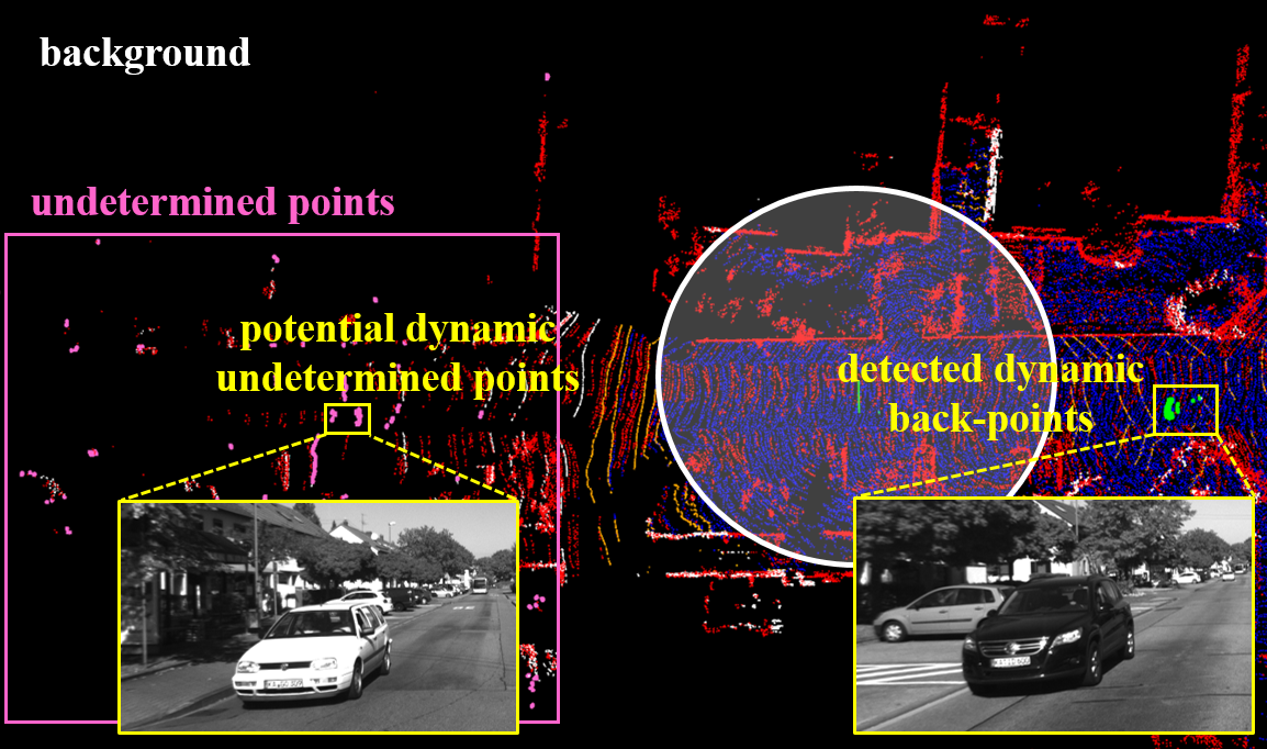
Figure 6: Visualization of dynamic point detection results for back-points.

Mode for back-points. If the number of nearest neighbors is below a certain threshold 5, we cannot ascertain whether it is due to a dynamic point not finding a nearest neighbor or because the location has not yet been reconstructed, thus preventing the search for a nearest neighbor. Such points are labeled as undetermined-points, and a determination will be made once the vehicle platform continues to move and the geometric structure of the location of these points is recovered. To ensure that newly acquired point clouds can be properly registered during state estimation, it is necessary to incorporate the undetermined-points into the tracking map. This will not significantly affect the accuracy of state estimation, as even if there are dynamic objects among the back-points, the number of LiDAR points scanned onto them is very sparse. As for the final output-map, it is imperative to ensure that it contains as few dynamic points as possible, hence the determination for undetermined-points will be conducted subsequently. When the number of nearest neighbors is sufficiently large (greater than 5), the processing approach is the same as that for fore-points, and the static points are added to both the tracking-map and the output-map. The visualization of dynamic point detection results for back-points is shown in Fig. 6.

Figure 7: Visualization of dynamic point detection results for undetermined-points.

Mode for undetermined-points. As the vehicle platform continues to move forward, the geometric structure information of previously unreconstructed positions in the global map is recovered (as shown in Fig. 7). When a point $\mathbf{p}_{u}^{w}$ in the undetermined points container is close to the current position of the vehicle platform (less than 30m), it is highly likely that the geometric structure information around $\mathbf{p}_{u}^{w}$ has been reconstructed. We can then determine whether $\mathbf{p}_{u}^{w}$ is a dynamic point. If the number of nearest neighbors is below a certain threshold 5, it suggests that the location of $\mathbf{p}_{u}^{w}$ was originally unoccupied, leading to the classification of $\mathbf{p}_{u}^{w}$ as a dynamic point. If the number of nearest neighbors is larger than 5, we calculate the proportion of non-ground points among all nearest neighbors. If this proportion is sufficiently smaller than 30$\%$, it is classified as a static point and added to the output-map. On the contrary, if the proportion is not smaller than 30$\%$, it is classified as a dynamic point and is not included. If an undetermined-point is more than 30m away from the vehicle platform’s position for 10 consecutive sweeps, it is directly classified as a static point and added to the output-map.

VI Experiments

We evaluated the overall performance of our method on three autonomous driving scenario datasets: Semantic-KITTI [1], ULHK-CA [17], and UrbanNav [7]. Semantic-KITTI is collected by a 64-line Velodyne LiDAR and each LiDAR point has its unique semantic label. Thus, Semantic-KITTI is used to evaluate the preservation rate (PR) and rejection rate (RR) of proposed label consistency based dynamic point detection and removal method. ULHK-CA is collected by a 32-line Robosense LiDAR and IMU, and UrbanNav is collected by a 32-line Velodyne LiDAR and IMU. These two datasets are used to evaluate the improvement of dynamic point detection and removal for pose estimation in terms of absolute trajectory error (ATE). A consumer-level computer equipped with an Intel Core i7-11700 and 32 GB RAM is used for all experiments.

VI-A PR and RR Comparison with the State-of-the-Arts

We compare our label consistency based dynamic point detection and removal method with three state-of-the-art 3D point-based dynamic point detection and removal methods, i.e., Removert [9], Erasor [10] and Dynamic Filter [6], on Semantic-KITTI dataset [1]. Among them, Removert and Erasor are offline methods which need the pre-built map as input, Dynamic Filter and Ours are online methods which do not rely on any prior information.

TABLE I: PR Comparison with State-of-the-Art Methods on Semantic-KITTI Dataset (unit: $\%$)

	offline		online
	Removert	Erasor	Dynamic Filter	Ours
Semantic-KITTI-00	86.83	93.98	90.07	90.36
Semantic-KITTI-01	95.82	91.49	87.95	88.43
Semantic-KITTI-02	83.29	87.73	88.02	88.25
Semantic-KITTI-05	88.17	88.73	90.17	90.31
Semantic-KITTI-07	82.04	90.62	87.94	89.28

TABLE II: RR Comparison with State-of-the-Art Methods on Semantic-KITTI Dataset (unit: $\%$)

	offline		online
	Removert	Erasor	Dynamic Filter	Ours
Semantic-KITTI-00	90.62	97.08	91.09	90.73
Semantic-KITTI-01	57.08	95.38	87.69	88.41
Semantic-KITTI-02	88.37	97.01	86.10	86.22
Semantic-KITTI-05	79.98	98.26	84.65	85.84
Semantic-KITTI-07	95.50	99.27	86.80	87.34

Results in Table I and Table II demonstrate that our label consistency based dynamic point detection and removal method outperforms Dynamic Filter for almost all sequences in terms of higher PR and RR. Although Dynamic Filter achieves higher RR than our method on sequence 00, our result is very close to theirs, with only a 0.36$\%$ difference.

VI-B ATE Comparison with the State-of-the-Arts

We integrate the proposed dynamic point detection and removal method into a self-designed LIO system to obtain Dynamic-LIO, and compare our Dynamic-LIO with four state-of-the-art LIO systems, i.e., LIO-SAM [15], Fast-LIO2 [20], RF-LIO [11] and ID-LIO [18], on ULHK-CA [17] and UrbanNav [7] datasets. LIO-SAM is a classic optimization-based LIO framework, and Fast-LIO2 is the state-of-the-art ESIKF-based LIO framework. RF-LIO and ID-LIO are LIO systems designed for handle dynamic environments. Both LIO-SAM, RF-LIO, ID-LIO and our Dynamic-LIO have loop detection module, and use GTSAM [8] to optimize the factor graph. We selected four sequences that encompass highly dynamic scenarios for evaluation, where $MarktStreet$ and $RussianHill$ are from ULHK-CA dataset, $TST$ and $Whampoa$ are from UrbanNav dataset.

TABLE III: ATE Comparison with State-of-the-Art Methods on ULHK-CA and UrbanNav Datasets (unit: m)

	LIO- SAM	Fast- LIO2	RF- LIO	ID- LIO	Ours
CA-MarktStreet	86.69	$\times$	15.89	28.02	12.96
CA-RussianHill	60.35	110.37	12.17	15.34	4.84
UrbanNav-TST	7.51	9.34	-	1.06	3.90
UrbanNav-Whampoa	3.32	5.38	-	3.45	6.66

• Denotations: ”$\times$” means the system drifts halfway through the corresponding sequence, ”-” means the corresponding value is not available.

Results in Table III demonstrate that the accuracy of our Dynamic-LIO is superior to that of LIO-SAM, Fast-LIO2, RF-LIO and ID-LIO on $MarktStreet$ and $RussianHill$. Since RF-LIO is neither open-sourced nor tested on the UrbanNav dataset, we are unable to obtain its results on sequence $TST$ and $Whampoa$. Although ID-LIO achieves smaller ATE than our system on UrbanNav dataset, our act of open-sourcing the code better substantiates the reproducibility of our results.

VI-C Ablation Study of Undetermined-Points

In our system, the purpose of incorporating undetermined-points is to remove dynamic points as much as possible, thereby increasing the proportion of static points in the output-map. In this section, we validate the necessity of incorporating undetermined-points through comparing the PR and RR value of our Dynamic-LIO with and without considering undetermined-points.

TABLE IV: Impact of Undetermined-Points on PR (unit: $\%$)

	Ours w/o considering undetermined-points	Ours
Semantic-KITTI-00	90.09	90.36
Semantic-KITTI-01	88.17	88.43
Semantic-KITTI-02	87.59	88.25
Semantic-KITTI-05	89.31	90.31
Semantic-KITTI-07	88.43	89.28

TABLE V: Impact of Undetermined-Points on RR (unit: $\%$)

	Ours w/o considering undetermined-points	Ours
Semantic-KITTI-00	90.05	90.73
Semantic-KITTI-01	87.86	88.41
Semantic-KITTI-02	86.22	86.22
Semantic-KITTI-05	84.08	85.84
Semantic-KITTI-07	87.30	87.34

Results in Table IV and Table V demonstrate that incorporating undetermined-points can slightly improve PR and RR of our dynamic point detection and removal method.

VI-D Ablation Study of Dynamic Point Removal for Pose Estimation

In this section, we evaluate the effectiveness of removing dynamic points for pose estimation by comparing the ATE result of our Dynamic-LIO with and without remove dynamic points.

TABLE VI: Impact of Removing Dynamic Points on ATE (unit: m)

	Ours w/p Removing Dynamic Points	Ours
CA-MarktStreet	13.98	12.96
CA-RussianHill	4.88	4.84
UrbanNav-TST	5.21	3.90
UrbanNav-Whampoa	9.19	6.66

Results in Table VI demonstrate that removing dynamic points can significantly enhance the pose estimation accuracy of our Dynamic-LIO.

VI-E Time Consumption Comparison with the State-of-the-Arts

We compare the time consumption of our label consistency based dynamic point detection and removal method with two state-of-the-art 3D point-based dynamic point detection and removal methods, i.e., Dynamic Filter [6] and RH-Map [22], on Semantic-KITTI dataset [1]. Then, we compare the time consumption of our Dynamic-LIO with RF-LIO and ID-LIO. Both results of other approaches are recorded from their literature.

TABLE VII: Time Consumption Comparison with State-of-the-Art Methods on Semantic-KITTI Dataset (unit: ms)

	Dynamic Filter (Front-End)	RH-Map	Ours
Semantic-KITTI-00	55.71	63.96	41.60
Semantic-KITTI-01		93.23	34.93
Semantic-KITTI-02		66.98	46.00
Semantic-KITTI-05		64.61	34.87
Semantic-KITTI-07		51.02	27.61

TABLE VIII: Time Consumption Comparison with State-of-the-Art LIO Systems on ULHK-CA and UrbanNav Datasets (unit: ms)

	RF-LIO	ID-LIO	Ours
CA-MarktStreet	96	121	23.33
CA-RussianHill	121	100	21.50
UrbanNav-TST	-	96	16.46
UrbanNav-Whampoa	-	99	16.41

• Denotations: ”-” means the corresponding value is not available.

TABLE IX: Time Consumption of Each Module (unit: ms)

	Cloud Processing	State Estimation	Dynamic Point Removal			Sum
			Ground Fitting	Label Consistency Detection	Total
Semantic-KITTI-00	7.49	27.98	1.85	4.28	6.13	41.60
Semantic-KITTI-01	2.01	24.57	1.84	6.51	8.35	34.93
Semantic-KITTI-02	7.11	36.07	1.88	0.94	2.82	46.00
Semantic-KITTI-05	7.66	18.93	1.85	6.43	8.28	34.87
Semantic-KITTI-07	7.94	19.67	1.80	1.21	3.01	27.61
CA-MarktStreet	5.45	13.48	0.53	3.87	4.40	23.33
CA-RussianHill	8.30	13.20	0.68	0.45	1.13	21.50
UrbanNav-TST	6.07	7.31	1.27	1.81	3.08	16.46
UrbanNav-Whampoa	7.14	7.03	1.33	0.91	2.24	16.41

Results in Table VII demonstrate that the time consumption of our dynamic point detection and removal method is much smaller than Dynamic Filter and RH-Map. The front-end of Dynamic Filter requires 55.71ms to process the data of a single sweep. When accounting for the back-end overhead, the total duration for processing a single sweep will be even longer. Given that the current LiDAR acquisition frequency is typically between 10$\sim$20Hz, this implies that the processing time for a single sweep must be within 50ms to ensure the real-time performance. It can be seen that neither Dynamic Filter nor RH-Map can guarantee real-time capability, whereas our method can rum in real time stably. Results in Table VIII demonstrate that the time consumption of our Dynamic-LIO is much smaller than RF-LIO [11] and ID-LIO [18], while our system operates at a speed approximately 5X faster than that of RF-LIO and ID-LIO. Since RF-LIO is neither open-sourced nor tested on the UrbanNav dataset, we are unable to obtain its results on sequence $TST$ and $Whampoa$.

VI-F Time Consumption of Each Module

We evaluate the runtime breakdown (unit: ms) of our system and for all testing sequences. For each sequence, we test the time consumption of cloud processing (except for ground fitting), state estimation and dynamic point removal. The dynamic point removel module can be further decomposed into two sub-steps: ground fitting and label consistency detection. Results in Table IX show that our system takes only 1$\sim$9ms to remove dynamic points of a sweep, while the total duration for completing other tasks of LIO is 16$\sim$46ms. This implies that our method can accomplish the dynamic point detection and removal with extremely low computational overhead in LIO systems.

VI-G Visualization for Map

Figure 8: Visualization of (a) output map before removing dynamic points and (b) output map after removing dynamic points.

Fig. 8 shows the ability of our Dynamic-LIO to reconstruct a static point cloud map on the exemplar sequence (e.g., semantic-KITTI-05). As illustrated in Fig. 8 (a), before removing dynamic points, the ghost tracks of moving objects (green points) are clearly visible on the map. As illustrated in Fig. 8 (b), after removing dynamic points, the output map almost no longer contains ghost tracks.

VII Conclusion

This paper proposes a label consistency based dynamic point detection and removal method, which determines whether a specific point is dynamic point based on the consistency with its nearest neighbors. We embed the proposed dynamic point detection and removal method into a self-designed LIO, which can accurately estimate state and exclude the interference of dynamic objects with extremely low cost.

Experimental results show that the proposed label consistency based dynamic detection and removal method can achieve comparable PR and RR to state-of-the-art dynamic point detection and removal methods, while ensuring a lower computational cost. In addition, our Dynamic-LIO operates at a speed approximately 5X faster than state-of-the-art LIO systems for dynamic environments.

References

- [1] J. Behley, M. Garbade, A. Milioto, J. Quenzel, S. Behnke, C. Stachniss, and J. Gall, “Semantickitti: A dataset for semantic scene understanding of lidar sequences,” in Proceedings of the IEEE/CVF international conference on computer vision, 2019, pp. 9297–9307.
- [2] Y. Cai, W. Xu, and F. Zhang, “ikd-tree: An incremental kd tree for robotic applications,” arXiv preprint arXiv:2102.10808, 2021.
- [3] K. Chen, R. Nemiroff, and B. T. Lopez, “Direct lidar-inertial odometry: Lightweight lio with continuous-time motion correction,” in 2023 IEEE International Conference on Robotics and Automation (ICRA). IEEE, 2023, pp. 3983–3989.
- [4] Z. Chen, K. Zhang, H. Chen, M. Y. Wang, W. Zhang, and H. Yu, “Dorf: A dynamic object removal framework for robust static lidar mapping in urban environments,” IEEE Robotics and Automation Letters, 2023.
- [5] P. Dellenbach, J.-E. Deschaud, B. Jacquet, and F. Goulette, “Ct-icp: Real-time elastic lidar odometry with loop closure,” in 2022 International Conference on Robotics and Automation (ICRA). IEEE, 2022, pp. 5580–5586.
- [6] T. Fan, B. Shen, H. Chen, W. Zhang, and J. Pan, “Dynamicfilter: an online dynamic objects removal framework for highly dynamic environments,” in 2022 International Conference on Robotics and Automation (ICRA). IEEE, 2022, pp. 7988–7994.
- [7] L.-T. Hsu, N. Kubo, W. Wen, W. Chen, Z. Liu, T. Suzuki, and J. Meguro, “Urbannav: An open-sourced multisensory dataset for benchmarking positioning algorithms designed for urban areas,” in Proceedings of the 34th International Technical Meeting of the Satellite Division of The Institute of Navigation (ION GNSS+ 2021), 2021, pp. 226–256.
- [8] M. Kaess, H. Johannsson, R. Roberts, V. Ila, J. J. Leonard, and F. Dellaert, “isam2: Incremental smoothing and mapping using the bayes tree,” The International Journal of Robotics Research, vol. 31, no. 2, pp. 216–235, 2012.
- [9] G. Kim and A. Kim, “Remove, then revert: Static point cloud map construction using multiresolution range images,” in 2020 IEEE/RSJ International Conference on Intelligent Robots and Systems (IROS). IEEE, 2020, pp. 10 758–10 765.
- [10] H. Lim, S. Hwang, and H. Myung, “Erasor: Egocentric ratio of pseudo occupancy-based dynamic object removal for static 3d point cloud map building,” IEEE Robotics and Automation Letters, vol. 6, no. 2, pp. 2272–2279, 2021.
- [11] C. Qian, Z. Xiang, Z. Wu, and H. Sun, “Rf-lio: Removal-first tightly-coupled lidar inertial odometry in high dynamic environments,” arXiv preprint arXiv:2206.09463, 2022.
- [12] C. Qin, H. Ye, C. E. Pranata, J. Han, S. Zhang, and M. Liu, “Lins: A lidar-inertial state estimator for robust and efficient navigation,” in 2020 IEEE international conference on robotics and automation (ICRA). IEEE, 2020, pp. 8899–8906.
- [13] L. Schmid, O. Andersson, A. Sulser, P. Pfreundschuh, and R. Siegwart, “Dynablox: Real-time detection of diverse dynamic objects in complex environments,” IEEE Robotics and Automation Letters, 2023.
- [14] T. Shan and B. Englot, “Lego-loam: Lightweight and ground-optimized lidar odometry and mapping on variable terrain,” in 2018 IEEE/RSJ International Conference on Intelligent Robots and Systems (IROS). IEEE, 2018, pp. 4758–4765.
- [15] T. Shan, B. Englot, D. Meyers, W. Wang, C. Ratti, and D. Rus, “Lio-sam: Tightly-coupled lidar inertial odometry via smoothing and mapping,” in 2020 IEEE/RSJ international conference on intelligent robots and systems (IROS). IEEE, 2020, pp. 5135–5142.
- [16] H. W. Sorenson, “Kalman filtering techniques,” in Advances in control systems. Elsevier, 1966, vol. 3, pp. 219–292.
- [17] W. Wen, Y. Zhou, G. Zhang, S. Fahandezh-Saadi, X. Bai, W. Zhan, M. Tomizuka, and L.-T. Hsu, “Urbanloco: A full sensor suite dataset for mapping and localization in urban scenes,” in 2020 IEEE international conference on robotics and automation (ICRA). IEEE, 2020, pp. 2310–2316.
- [18] W. Wu and W. Wang, “Lidar inertial odometry based on indexed point and delayed removal strategy in highly dynamic environments,” Sensors, vol. 23, no. 11, p. 5188, 2023.
- [19] J. R. Xu, S. Huang, S. Qiu, L. Zhao, W. Yu, M. Fang, M. Wang, and R. Li, “Lidar-link: Observability-aware probabilistic plane-based extrinsic calibration for non-overlapping solid-state lidars,” IEEE Robotics and Automation Letters, 2024.
- [20] W. Xu, Y. Cai, D. He, J. Lin, and F. Zhang, “Fast-lio2: Fast direct lidar-inertial odometry,” IEEE Transactions on Robotics, vol. 38, no. 4, pp. 2053–2073, 2022.
- [21] W. Xu and F. Zhang, “Fast-lio: A fast, robust lidar-inertial odometry package by tightly-coupled iterated kalman filter,” IEEE Robotics and Automation Letters, vol. 6, no. 2, pp. 3317–3324, 2021.
- [22] Z. Yan, X. Wu, Z. Jian, B. Lan, and X. Wang, “Rh-map: Online map construction framework of dynamic object removal based on 3d region-wise hash map structure,” IEEE Robotics and Automation Letters, 2023.
- [23] Z. Yuan, J. Deng, R. Ming, F. Lang, and X. Yang, “Sr-livo: Lidar-inertial-visual odometry and mapping with sweep reconstruction,” IEEE Robotics and Automation Letters, vol. 9, no. 6, pp. 5110–5117, 2024.
- [24] Z. Yuan, F. Lang, T. Xu, and X. Yang, “Sr-lio: Lidar-inertial odometry with sweep reconstruction,” arXiv preprint arXiv:2210.10424, 2022.
- [25] Z. Yuan, F. Lang, T. Xu, C. Zhao, and X. Yang, “Semi-elastic lidar-inertial odometry,” arXiv preprint arXiv:2307.07792, 2023.
- [26] Z. Yuan, Q. Wang, K. Cheng, T. Hao, and X. Yang, “Sdv-loam: Semi-direct visual–lidar odometry and mapping,” IEEE Transactions on Pattern Analysis and Machine Intelligence, vol. 45, no. 9, pp. 11 203–11 220, 2023.