FDS: Feedback-guided Domain Synthesis with Multi-Source Conditional Diffusion Models for Domain Generalization

Abstract

Domain Generalization techniques aim to enhance model robustness by simulating novel data distributions during training, typically through various augmentation or stylization strategies. However, these methods frequently suffer from limited control over the diversity of generated images and lack assurance that these images span distinct distributions. To address these challenges, we propose FDS, Feedback-guided Domain Synthesis, a novel strategy that employs diffusion models to synthesize novel, pseudo-domains by training a single model on all source domains and performing domain mixing based on learned features. By incorporating images that pose classification challenges to models trained on original samples, alongside the original dataset, we ensure the generation of a training set that spans a broad distribution spectrum. Our comprehensive evaluations demonstrate that this methodology sets new benchmarks in domain generalization performance across a range of challenging datasets, effectively managing diverse types of domain shifts. The implementation is available at: https://github.com/Mehrdad-Noori/FDS.git.

1 Introduction

Deep learning architectures, including Convolutional Neural Networks (CNNs) and Vision Transformers (ViTs), have significantly advanced the field of computer vision, achieving state-of-art results in tasks like classification, semantic segmentation, and object detection. Despite these advancements, such models commonly operate under the simplistic assumption that training data (source domain) and post-deployment data (target domain) share identical distributions. This overlook of distributional shifts results in performance degradation when models are exposed to out-of-distribution (OOD) data [1, 2]. Domain adaptation (DA) [3, 4, 5] and Test-Time Adaptation (or Training) [6, 7, 8] strategies have been developed to mitigate this issue by adjusting models trained on the source domain to accommodate a predefined target domain. Nonetheless, these strategies are constrained by their dependence on accessible target domain data for adaptation, a prerequisite that is not always feasible in real-world applications. Furthermore, adapting models to each novel target domain entails considerable computational overhead, presenting a practical challenge to their widespread implementation.

Domain generalization (DG) [9] aims to solve the issue of domain shift by training models using data from one or more source domains, so they perform well out-of-the-box on new, unseen domains. Recently, various techniques have been developed to tackle this problem [10, 11], including domain aligning [12, 13, 14], meta-learning [15, 16], data augmentation [17, 18, 19], ensemble learning[20], self-supervised learning [21, 22], and regularization methods [23, 24]. These strategies are designed to make models more adaptable and capable of handling data that they were not explicitly trained on, making them more useful in real-world situations where the exact nature of future data cannot be predicted. Among these techniques, a notable category focuses on synthesizing samples from different distributions to mimic target distributions. This is achieved through strategies like image transformation [17, 25], style transfer [26, 27], learnable augmentation networks [28, 29, 30], and feature-level stylization [20, 31]. However, many of these methods face challenges in controlling the synthesis process, often resulting in limited diversity where primarily only textures are altered.

Figure 1: Generating new, pseudo-domains with FDS: Comprehensive distribution coverage from domain $D_{1}$ to $D_{2}$.

In this study, we introduce an innovative approach using diffusion model, named Feedback-guided Domain Synthesis (FDS), to address the challenge of domain generalization. Known for their exceptional ability to grasp intricate distributions and semantics, diffusion models excel at producing high-quality, realistic samples [32, 33, 34, 35]. We exploit this strength by training a single diffusion model that is conditioned on various domains and classes present in the training dataset, aiming to master the distribution of source domains. As illustrated in Figure 1, through the process of domain interpolation and mixing during generation, we create images that appear to originate from novel, pseudo-domains. To ensure the development of a robust classifier, we initially select generated samples that are difficult for a model trained solely on the original source domains to classify. Subsequently, we train the model using a combination of these challenging images and the original dataset. In this manner, we ensure that our model is fed with images of the widest possible diversity, thereby significantly enhancing its ability to generalize across unseen domains. Our contributions can be summarized as follows:

• We introduce a novel DG approach that leverages diffusion models conditioned on multiple domains and classes to generate samples from novel, pseudo-domains through domain interpolation. This approach increases the diversity and realism of the generated images;

• We propose an innovative strategy for selecting images that pose a challenge to a classifier trained on original images, ensuring the diversity of the final sample set. By incorporating these challenging images with the original dataset, we ensure a comprehensive and diverse training set, significantly improving the model’s generalization capabilities;

• We conduct extensive experiments across various benchmarks and perform different analyses to validate the effectiveness of our method. These experiments demonstrate FDS’s ability to significantly improve the robustness and generalization of models across a wide range of unseen domains, achieving SOTA performance.

2 Related Works

2.1 Domain Generalization (DG)

Domain Generalization, a concept first introduced by Blanchard et al. in 2011 [9], has seen growing interest in the field of computer vision. This interest has spurred the development of a broad spectrum of methods aimed at enabling models to generalize across unseen domains. These include approaches based on domain alignment like moment matching [36], discriminant analysis [12] and domain-adversarial learning [37], meta-learning approaches [15, 16] which solve a bi-level optimization problem where the model is fine-tuned on meta-source domains to minimize the error on a meta-target domain, ensemble learning techniques [20, 38] improving robustness to OOD data by training multiple models tailored to specific domains, self-supervised learning methods fostering domain-agnostic representations through the pre-training of models on unsupervised tasks [21, 39, 40] or via contrastive learning [41], approaches leveraging disentangled representation learning [42, 43] segregating domain-specific features from those common across all domains, and regularization methods which build on the empirical risk minimization (ERM) framework [44], incorporating additional objectives such as distillation [45, 46], stochastic weight averaging [24], or distributionally robust optimization (DRO) [47] to promote generalization.

A key strategy in DG, data augmentation aims to enhance model robustness against domain shifts encountered during deployment. This objective is pursued through a variety of techniques, such as learnable augmentation, off-the-shelf style transfer, and augmentation at the feature level. Learnable augmentation models utilizes networks to create images from training data, ensuring their distribution diverges from that of the source domains [28, 30, 29]. Meanwhile, off-the-shelf style transfer based methods seek to transform the appearance of images from one domain to another or modify their stylistic elements, often through Adaptive Instance Normalization (AdaIN)[48, 26]. Unlike most augmentation approaches that modify pixel values, some propose altering features directly, a technique inspired by the finding that CNN features encapsulate style information[49, 20] in their statistics.

2.2 Diffusion Models

Diffusion models have recently surpassed Generative Adversarial Networks (GANs) as the leading technique for image synthesis. Innovations like denoising diffusion probabilistic models (DDPMs) [33] and denoising diffusion implicit models (DDIMs) [35] have significantly sped up the image generation process. Rombach et al. [34] introduced latent diffusion models (LDMs), also known as stable diffusion models, which enhance both training and inference efficiency while facilitating text-to-image and image-to-image conversions. Extensions of these models, such as stable diffusion XL (SDXL) [50] and ControlNet [51], have been developed to further guide the generation process with additional inputs, such as depth or semantic information, allowing for more controlled and versatile image creation. Recent studies have shown that augmenting datasets using diffusion models can improve performance in general vision tasks [52, 53].

Despite the capabilities of diffusion models in generating images, their application in domain generalization has been minimally explored. Yue et al. [54] proposed a method called DSI to address OOD prediction by transforming testing samples back to the training distribution using multiple diffusion models, each trained on a single source distribution. While effective, DSI requires multiple models during prediction, making it impractical for real-time deployment. In contrast, our method only uses diffusion during training to synthesize pseudo-domains and select more challenging images, keeping the computational complexity the same during testing while achieving significantly better performance.

In another study, CDGA [55] uses diffusion models to generate synthetic images that fill the gap between different domain pairs through a simple interpolation. While effective, CDGA relies on generating a large number of synthetic images (e.g., 5M for PACS) and employs naive interpolation. Additionally, CDGA generates samples with additional text descriptions that are not provided in standard DG benchmarks. In contrast, our method employs novel and more efficient interpolation techniques and a unique filtering mechanism that selects challenging images. We demonstrate that both of these innovations are crucial and significantly effective for improving generalization.

Figure 2: Overview of the proposed architecture for FDS. (top) Multi-source training of diffusion model conditioned on class and domain of the training images. (bottom) Generating novel pseudo-domain using the proposed interpolation and filtering mechanism of FDS.

3 Theoretical Motivation

Our classifier, represented by $f$ with parameters $\theta$, aims to craft a unified model from $n$ source domains $\{\mathcal{D}^{1},\ldots,\mathcal{D}^{n}\}$ that adapts to a novel target domain $\mathcal{D}^{\mathcal{T}}$. Within any domain $\mathcal{D}$, we measure classification loss by

$$\mathcal{L}_{\mathcal{D}}(\theta)\,=\,\mathbb{E}_{(x,y)\sim\mathcal{D}}\,\big{[}\ell(f(x;\theta),y)\big{]},$$ (1)

where $x$ and $y$ denote the input and its corresponding label, respectively, and $\ell(f(x;\theta),y)$ is the cross entropy loss in this work.

Empirical Risk Minimization (ERM) [56] forms the foundation for training our models, aiming to reduce the mean loss across training domains:

$$\min_{\theta}\ \sum_{i}\frac{1}{|\mathcal{D}^{i}|}\sum_{k=1}^{|\mathcal{D}^{i}|}\ell(f(x_{i}^{k};\theta),y_{i}^{k})$$ (2)

Here, $|\mathcal{D}^{i}|$ counts the number of samples in domain $i$, with $x_{i}^{k}$ as the $k$-th sample and $y_{i}^{k}$ its label. However, the accuracy of ERM-trained models drops when data shifts occur across domains due to inadequate OOD generalization. To enhance ERM, Chapelle et al. introduced Vicinal Risk Minimization (VRM) [57], which substitutes point-wise estimates with density estimation in the vicinity distribution around each observation within each domain. Practical implementation often involves data augmentation to introduce synthetic samples from these density estimates. Traditional augmentation processes a single data point $\tilde{x}_{i}^{k}$ from domain $i$ to yield $\tilde{x}_{i}^{k}=g(\tilde{x}_{i}^{k})$, where $g(\cdot)$ denotes a basic transformation and $\tilde{x}_{i}^{k}$ is the modified data point.

Despite the potential of VRM to boost performance on OOD samples, it does not completely bridge domain gaps. The root cause lies in the inability of ERM methods to anticipate shifts in data distribution, which simple augmentation within domains does not address. Hence, domain generalization requires more robust transformations to extend the model’s applicability beyond training domains. Muller et al. [58] have demonstrated that a wider range of transformations outperforms standard methods. However, Aminbeidokhti et al. [59] advise that aggressive augmentations could distort the essential characteristics of images, pointing to the necessity of a mechanism to filter out extreme alterations. The emergence of diffusion models, proficient in reproducing diverse data distributions, facilitates such advanced sampling approaches. Our goal, therefore, is to generate images that span across domain gaps, lessen the variability between data distributions, and introduce a system to exclude trivial or excessive modifications.

4 Method

To advance the generalization ability of our classifier, we aim to utilize generated image samples that traverse domain gaps yet retain class semantics. This objective is realized through a three-step methodology of our proposed method FDS. Step 1: we begin by training an image generator that masters the class-specific distributions of all source domains, enabling the synthesis of class-consistent samples within those domains. Step 2: we then introduce a strategy for generating inter-domain images to span the domain gaps effectively. Step 3: last, we filter overly simplistic samples from synthetic inter-domain images and train the final model on this refined set alongside original domain images for enhanced OOD generalization. The process is illustrated in Figure 2.

4.1 Image Generator

Diffusion Models are designed to approximate the data distribution $p(x)$ by reversing a predefined Markov Chain of $T$ steps, effectively denoising a sample in stages. These stages are modeled as a sequence of denoising autoencoder applications $e_{\theta}(x_{t},t)$, for $t=1\ldots T$, which gradually restore their input $x_{t}$. This iterative restoration is formalized by the following objective:

$$\mathcal{L}_{DM}\,=\,\mathbb{E}_{x,\epsilon\sim\mathcal{N}(0,1),\,t}\left[\|\epsilon-\epsilon_{\theta}(x_{t},t)\|^{2}\right],$$ (3)

where $t$ is drawn uniformly from $\{1,\ldots,T\}$. Utilizing perceptual compression models, encoded by $\mathcal{E}$ and decoded by $\mathcal{\tilde{E}}$, we access a latent space that filters out non-essential high-frequency details. By placing the diffusion process in this compressed space, our objective is then reformulated as

$$\mathcal{L}_{LDM}\,=\,\mathbb{E}_{\mathcal{E}(x),\epsilon\sim\mathcal{N}(0,1),\,t}\left[\left\|\epsilon-\epsilon_{\theta}(z_{t},t)\right\|^{2}\right].$$ (4)

Diffusion models can also handle conditional distributions $p(z|c)$. To enable this conditioning, building upon the work of Rombach et al. [34], we utilize a condition encoder $\tau_{\theta}$ that maps $c$ onto an intermediate representational space $\tau(c)\in\mathbb{R}^{M\times d_{\tau}}$. Following Stable Diffusion, we employ the CLIP-tokenizer and implement $\tau$ as a transformer to infer a latent code. This representation is subsequently integrated into the UNet using a cross-attention mechanism, culminating in our final enhanced objective:

$$\mathcal{L}_{LDM}^{\mathrm{cond}}\,=\,\mathbb{E}_{\mathcal{E}(x),\,c,\,\epsilon\sim\mathcal{N}(0,1),\,t}\left[\left\|\epsilon-\epsilon_{\theta}(z_{t},t,\tau(c))\right\|^{2}\right],$$ (5)

This approach enables a single diffusion model to understand and generate images across different domains for each class, using text-based conditions (prompts). By dynamically adjusting conditions, the model efficiently learns varied representations without needing multiple models for each domain. Thus, we employ a textual template $c(x)$, denoting “[y], [D]” where y is the class label and D is the domain name of the input $x$, and proceed to train our diffusion model using this template across all images from the source domains. Upon completing training, we can create a new sample for class $y^{k}$, belonging to the set $\{y^{1},\ldots,y^{m}\}$, within domain $\mathcal{D}^{i}$. This is achieved by decoding a denoised representation after $t$ timesteps, $\tilde{x}_{t}^{i,k}=\tilde{\mathcal{E}}(\Phi_{t}(\mathcal{D}^{i},y^{k}))$, where $\Phi_{t}(\mathcal{D}^{i},y^{k})$ is the denoised representation that originates from random Gaussian noise conditioned on $\mathcal{D}^{i}$ and $y^{k}$.

4.2 Domain Mixing

We propose two mixing strategies to synthesize images from new, pseudo distributions, based on noise-level interpolation and condition-level interpolation.

4.2.1 Noise Level Interpolation

Consider our dataset comprising $n$ source domains $\{\mathcal{D}^{1},\ldots,\mathcal{D}^{n}\}$ and target classes $y^{k}$ from the set $\{y^{1},\ldots,y^{m}\}$. Utilizing a trained image generator that initiates with random Gaussian noise, we denoise this input over $t$ steps to produce a synthetic, denoised representation $\tilde{z}_{t}^{i,k}=\Phi_{t}(\mathcal{D}^{i},y^{k})$ indicative of domain $\mathcal{D}^{i}$ and class $y^{k}$. To synthesize a sample that merges the characteristics of domains $\mathcal{D}^{i}$ and $\mathcal{D}^{j}$ for class $y^{k}$, we employ a single diffusion model, conditioned dynamically to capture the essence of both domains. This process aims to generate a sample that embodies the transitional features between these domains, effectively bridging the domain gap.

The model begins its process from the same initial random Gaussian noise, adapting its denoising trajectory under two distinct conditions, $\tau(\mathcal{D}^{i},y^{k})$ and $\tau(\mathcal{D}^{j},y^{k})$, up to a specific timestep $T$. This dual-conditioned approach ensures that the evolving representation up to $T$ incorporates influences from both domains, guided by the respective conditional inputs.

From timestep $T$ onwards, until the final representation is formed, the model blends the outputs from these dual paths at each step. Specifically, for each step $t>T$, we form a mixed representation $\tilde{z}_{t}$ as:

$$\tilde{z}_{t}\,=\,\alpha\,\Phi_{t}(\mathcal{D}^{i},y^{k})\,+\,(1\!-\!\alpha)\,\Phi_{t}(\mathcal{D}^{j},y^{k}),$$ (6)

where $\alpha$ is a predefined mixing coefficient that dictates the blend of domain characteristics in the output. This combined representation $\tilde{z}_{t}$ is then used as the basis for the model’s next denoising step, integrating features from both $\mathcal{D}^{i}$ and $\mathcal{D}^{j}$ for class $y^{k}$. Through this iterative mixing, the model ensures a gradual and cohesive fusion of domain-specific attributes, leading to a synthesized sample that seamlessly spans the gap between the domains for class $y^{k}$.

4.2.2 Condition Level Interpolation

We also propose Condition Level Interpolation to generate images that effectively bridge domain gaps. This technique relies on manipulating the conditions fed into our diffusion model to guide the synthesis of new samples. Specifically, for a target class $y^{k}$ and two distinct domains, $\mathcal{D}^{i}$ and $\mathcal{D}^{j}$, we employ our encoder $\tau(c)$ to create separate condition representations for each domain-class pair: $(y^{k},\mathcal{D}^{i})$ and $(y^{k},\mathcal{D}^{j})$.

The core of this strategy involves blending these condition representations using a mix coefficient $\alpha$, leading to a unified condition:

$$c_{\mathrm{mixed}}\,=\,\alpha\,\tau(c_{y^{k}},\mathcal{D}^{i})\,+\,(1\!-\!\alpha)\,\tau(c_{y^{k}},\mathcal{D}^{j}).$$ (7)

This mixed condition $c_{\text{mixed}}$ then orchestrates the generation process from the initial step, ensuring that the diffusion model is consistently influenced by attributes from both domains. By initiating this conditioned blending from the beginning of the diffusion process, we ensure a harmonious integration of domain characteristics throughout the generation of the synthetic image.

4.3 Filtering Mechanism

Through our mixing strategies, we create synthetic samples $\tilde{x}_{i,j}^{k}$ that not only synthesize class $y^{k}$ traits but also blend features from domains $\mathcal{D}^{i}$ and $\mathcal{D}^{j}$, thereby aiming to bridge the domain gaps. This approach generates a synthetic dataset comprising $\tilde{N}$ samples for each combination of class index $k$ and domain index pair $(i,j)$, structured as $S_{i,j}^{k}=\{\tilde{x}_{i,j}^{k,(r)}\,|\,1\leq i<j\leq n,\,\,1\leq k\leq m,\,\,1\leq r\leq\tilde{N}\}$, ensuring diversity via distinct random Gaussian noise initiation for each sample.

The utility of these synthetic samples in improving model generalization varies, prompting an entropy-based evaluation to identify those with the greatest potential. High entropy scores, indicating prediction uncertainty by a classifier $h(x)$ trained on the original dataset, suggest that such samples may come from previously unseen distributions. This characteristic posits these high-entropy samples as prime candidates for training, hypothesized to challenge the classifier significantly and aid in covering the domain gaps. Further refining this selection, we only include samples correctly predicted as their target class by $h(x)$, ensuring the exclusion of samples that have lost semantic integrity during the diffusion process.

Let $\mathcal{C}_{i,j}^{k}$ be the subset of samples in $S_{i,j}^{k}$ with are correctly classified by $h(x)$:

$$\mathcal{C}_{i,j}^{k}\,=\,\big{\{}\tilde{x}_{i,j}^{k,(r)}\,|\,h(\tilde{x}_{i,j}^{k,(r)})=y^{k}\big{\}}.$$ (8)

We choose from $\mathcal{C}_{i,j}^{k}$ the $N_{L}$ samples with highest entropy (the entropy of a $k$-class discrete probability distribution $p$ is given by $\mathcal{H}(p)=-\sum_{k}p_{k}\log p_{k}$) to form a set of selected samples $\tilde{\mathcal{D}}_{i,j}^{k}$. Last, we combine the synthetic samples, created for each class and domain pair, to the original dataset $\mathcal{O}$ to obtain the final augmented training set

$$\mathcal{A}\,=\,\mathcal{O}\,\cup\,\big{\{}\tilde{\mathcal{D}}_{i,j}^{k}\,|\,1\leq i<j\leq n,\,\,1\leq k\leq m\big{\}}$$ (9)

Training the final classifier on $\mathcal{A}$ not only enriches the dataset but also ensures robust model generalization across diverse domain landscapes.

5 Experimental Setup

Table 1: Leave-one-out accuracy (%) results on the PACS, VLCS, and OfficeHome benchmarks. "Aug." indicates whether advanced augmentation or domain mixing techniques are used. The best results and second-best results are highlighted.

Method Aug. PACS VLCS Office  Avg. Standard Methods ERM (baseline) [44] ✗ 85.5 $\pm$0.2 77.5 $\pm$0.4 66.5 $\pm$0.3 76.5 ERM (reproduced) ✗ 84.3 $\pm$1.1 76.2 $\pm$1.1 64.6 $\pm$1.1 75.0 IRM [60] ✗ 83.5 $\pm$0.8 78.5 $\pm$0.5 64.3 $\pm$2.2 75.4 GroupDRO [47] ✗ 84.4 $\pm$0.8 76.7 $\pm$0.6 66.0 $\pm$0.7 75.7 Mixup [61] ✓ 84.6 $\pm$0.6 77.4 $\pm$0.6 68.1 $\pm$0.3 76.7 CORAL [62] ✗ 86.2 $\pm$0.3 78.8 $\pm$0.6 68.7 $\pm$0.3 77.9 MMD [63] ✗ 84.6 $\pm$0.5 77.5 $\pm$0.9 66.3 $\pm$0.1 76.1 DANN [64] ✗ 83.6 $\pm$0.4 78.6 $\pm$0.4 65.9 $\pm$0.6 76.0 SagNet [65] ✓ 86.3 $\pm$0.2 77.8 $\pm$0.5 68.1 $\pm$0.1 77.4 RSC [23] ✓ 85.2 $\pm$0.9 77.1 $\pm$0.5 65.5 $\pm$0.9 75.9 Mixstyle [20] ✓ 85.2 $\pm$0.3 77.9 $\pm$0.5 60.4 $\pm$0.3 74.5 mDSDI [66] ✗ 86.2 $\pm$0.2 79.0 $\pm$0.3 69.2 $\pm$0.4 78.1 SelfReg [41] ✓ 85.6 $\pm$0.4 77.8 $\pm$0.9 67.9 $\pm$0.7 77.1 DCAug [59] ✓ 86.1 $\pm$0.7 78.6 $\pm$0.4 68.3 $\pm$0.4 77.7 CDGA [55] ✓ 88.5 $\pm$0.5 79.6 $\pm$0.3 68.2 $\pm$0.6 78.8 ERM + FDS (ours) ✓ 88.8 $\pm$0.1 79.8 $\pm$0.5 71.1 $\pm$0.1 79.9 WA Methods SWAD (baseline) [24] ✗ 88.1 $\pm$0.1 79.1 $\pm$0.1 70.6 $\pm$0.2 79.3 SWAD (reproduced) ✗ 88.1 $\pm$0.4 78.9 $\pm$0.5 70.3 $\pm$0.4 79.1 SelfReg SWA [41] ✓ 86.5 $\pm$0.3 77.5 $\pm$0.0 69.4 $\pm$0.2 77.8 DNA [67] ✗ 88.4 $\pm$0.1 79.0 $\pm$0.1 71.2 $\pm$0.1 79.5 DIWA [68] ✓ 88.8 $\pm$0.4 79.1 $\pm$0.2 71.0 $\pm$0.1 79.6 TeachDCAug [59] ✓ 88.4 $\pm$0.2 78.8 $\pm$0.4 70.4 $\pm$0.2 79.2 SWAD + FDS (ours) ✓ 90.5 $\pm$0.3 79.7 $\pm$0.5 73.5 $\pm$0.4 81.3

Datasets.  Following [44], we compare our proposed approach to the current state-of-art using three challenging datasets - 12 individual target domains - with different characteristics: PACS [42], VLCS [69], and OfficeHome [70]. The PACS dataset has a total of 9,991 photos divided into four distinct domains, $d\in$ {Art, Cartoon, Photo, Sketch} and seven distinct classes. The second dataset, VLCS, comprises 10,729 photos from four separate domains, $d\in$ {Caltech101, LabelMe , SUN09, VOC2007} and five different classes. The third dataset, OfficeHome, includes a total of 15,588 photos taken from four domains, $d\in$ {Art, Clipart, Product, Real}, and 65 classes.

Implementation Details.  To ensure a fair comparison, we adopt the DomainBed framework [44], a comprehensive benchmark that encompasses prominent domain generalization (DG) methodologies under a uniform evaluation protocol. Following this framework, we employ a leave-one-out strategy for DG dataset assessment where one domain serves as the test set while the others form the training set. A subset of the training data, constituting 20%, is designated as the validation set. The aggregate result for each dataset represents the mean accuracy derived from varying the test domain. To ensure reliability, experiments are replicated three times, each with a unique seed. Moreover, to rigorously test our method, we try both ERM and SWAD classifiers with FDS. The former is considered a baseline in standard training methods, while the latter serves as a baseline for weight averaging (WA) methods. SWAD is essentially ERM but with weight averaging applied during training using multiple steps based on the validation set. To have a fair comparison with other methods, for the ERM baseline, we strictly follow the hyperparameter tuning proposed in [24]. For SWAD, as in the original work, we did not tune any parameters and used the default values. For image synthesis, the original Stable Diffusion framework [34] is utilized with $\mathrm{DDIM}\!=\!50$ steps. The PACS and VLCS datasets prompt the generation of $N\!=\!32,000$ samples per class, whereas OfficeHome, with its 65 classes, necessitates $N\!=\!16,000$ samples. Image generation spans an interpolation range of $\alpha\!\in\![0.3,0.7]$ and a Noise Level Interpolation range of $\mathcal{T}\!\in\![20,45]$. This diversified parameter selection, rather than optimizing hyperparameters per dataset, acknowledges each domain’s unique shift. Our filtering mechanism then identifies the most informative images from the generated pool. The selection of an optimal dataset size, $N_{L}$, underwent extensive exploration, detailed further in Section 6.2.

6 Results

We first compare the performance of our FDS approach against SOTA DG methods across three benchmarks. We then present a detailed analysis investigating several key aspects of our approach, including the effectiveness of each proposed component, a comparison of different mixing strategies, its regularization capabilities, domain diversity visualization and quantification, the impact of data size, the efficacy of our filtering mechanism, and stability analysis during training. Additional analysis, visualizations, and detailed tables can be found in the Supplementary Material.

6.1 Comparison with the State-of-the-art

In Table 1, we compare our approach with recent methods for domain generalization as outlined in the DomainBed framework [44]. Our method, when added to the baseline ERM classifier, shows an impressive improved accuracy of 4.5% on the PACS dataset using the ResNet-50 model. On the VLCS dataset, our method sees a 3.6% increase in accuracy over the ERM. For the OfficeHome dataset, our method outperforms the ERM baseline by 6.5%. To test the strength of our method, we also applied it to SWAD, which is a the baseline for weight averaging (WA) domain generalization methods. Here, our method improves the performance by 2.4%, 0.8%, and 3.2% on the PACS, VLCS, and OfficeHome datasets, respectively.

Furthermore, when comparing with previous SOTA methods, our method outperforms CDGA [55], by 0.3% on PACS, 0.2% on VLCS, and 2.9% on OfficeHome. In the context of weight averaging methods, our approach surpasses DIWA [68], which trains multiple independent models, by 1.7% on PACS, 0.6% on VLCS, and 2.5% on OfficeHome, setting a new benchmark for domain generalization. Please refer to the Supplementary Material for the full, detailed results for each dataset and its domains.

6.2 Further Analysis

For this section, we use the SWAD baseline to analyze the performance of our proposed method FDS, due to its stable performance as a WA method. Final settings are applied to the ERM baseline. All analyses in this section use the PACS dataset and the SWAD baseline unless otherwise stated.

Table 2: Comparative analysis of FDS component effects on accuracy (%) across PACS dataset domains. "Basic" refers to generation without interpolation or filtering.

Module Target Domains Art Cartoon Photo Sketch Avg. Baseline (SWAD [24]) 89.49 $\pm$0.2 83.65 $\pm$0.4 97.25 $\pm$0.2 82.06 $\pm$1.0 88.11 $\pm$0.4 + Basic 89.87 $\pm$0.1 85.59 $\pm$0.6 97.50 $\pm$0.3 83.07 $\pm$0.4 89.01 $\pm$0.4 + Interpolation 91.38 $\pm$0.2 85.20 $\pm$0.6 97.73 $\pm$0.1 84.27 $\pm$0.9 89.65 $\pm$0.4 + Filtering 91.80 $\pm$0.3 86.03 $\pm$0.8 98.05 $\pm$0.2 86.11 $\pm$0.1 90.50 $\pm$0.3

Ablation Study on Different Components.  To evaluate the impact of each component on generalization, we systematically introduce each module and observe the enhancements. As detailed in Table 2, first incorporating domain-specific synthetic samples, generated without interpolation or filtering (Basic), yields a $0.9\%$ gain over the baseline. This increment validates our diffusion model’s proficiency in capturing and replicating the class-specific distributions within domains, thus refining OOD performance through enhanced density estimation near original samples. Subsequently, integrating images from pseudo-novel domains via our interpolation strategy leads to a further $0.5\%$ enhancement, underscoring the mechanism’s effectiveness in connecting distinct domains. Lastly, applying our entropy-based filtering to eliminate overly simplistic images and images with diminished semantic relevance results in a significant $2.4\%$ improvement against the SWAD model, a robust benchmark. These outcomes collectively underscore the efficacy of our approach in improving OOD generalization.

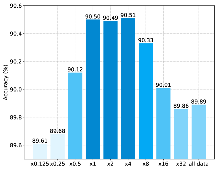
Figure 3: Impact of varying scales of sample size $N_{L}$ relative to the average number of images per class on PACS dataset.

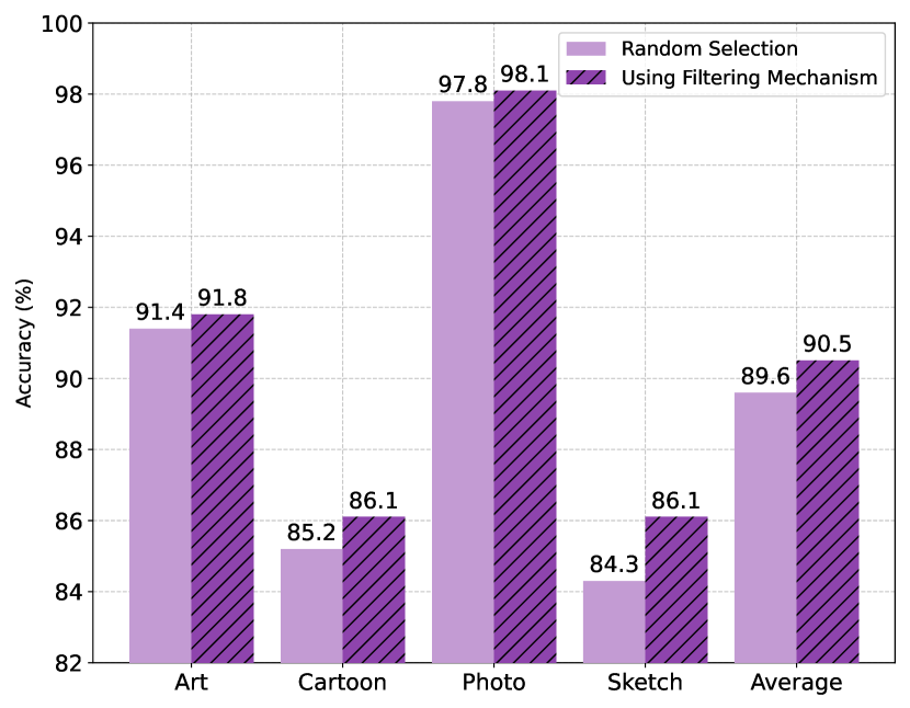
Figure 4: Impact of using Random Selection vs. Proposed Filtering Strategy of FDS on PACS accuracy (%).

Table 3: Impact of different interpolation strategies of FDS on PACS accuracy (%).

Strategy Target Domains Art Cartoon Photo Sketch Avg. Baseline (SWAD [24]) 89.49 $\pm$0.2 83.65 $\pm$0.4 97.25 $\pm$0.2 82.06 $\pm$1.0 88.11 $\pm$0.4 Noise Level Interpol. 91.95 $\pm$0.3 83.23 $\pm$0.1 97.56 $\pm$0.1 85.85 $\pm$0.3 89.65 $\pm$0.2 Condition Level Interpol. 91.80 $\pm$0.3 86.03 $\pm$0.8 98.05 $\pm$0.2 86.11 $\pm$0.1 90.50 $\pm$0.3 Both 91.13 $\pm$0.4 82.98 $\pm$0.2 97.90 $\pm$0.2 85.62 $\pm$0.8 89.41 $\pm$0.4

Mixing Strategies.  Our ablation study, presented in Table 3, reveals that both Noise Level Interpolation and Condition Level Interpolation significantly outperform the baseline, yet their effectiveness varies with the dataset’s attributes and the nature of the domain shift. Noise Level Interpolation is optimal for minimal domain shifts, focusing on adjusting the noise aspect to bridge domain gaps. However, it falls short in scenarios with substantial domain differences, such as the transition to Cartoon or Sketch, where the source and target domains diverge significantly. In these cases, Condition Level Interpolation proves more advantageous, offering a robust mechanism for navigating complex domain shifts by manipulating higher-level semantic representations. When applying both methods simultaneously, the performance did not improve compared to using Condition Level Interpolation alone, possibly due to the increased complexity. Nonetheless, it still performed better than the baseline. Based on these results, we use Condition Level Interpolation as our final interpolation method.

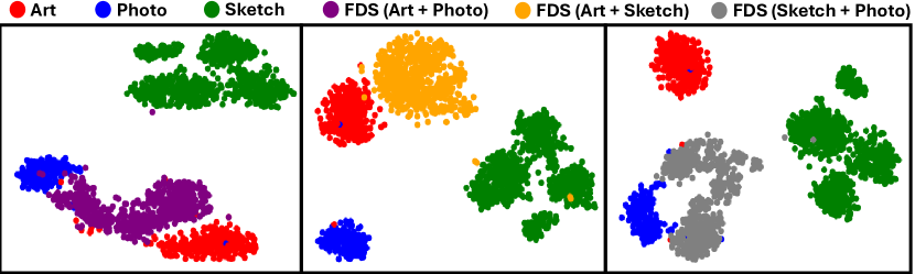
Figure 5: t-SNE plots showcasing the original and generated samples for the "Art", "Photo", and "Sketch" source domains and the "giraffe" class in the PACS dataset using our method. Features were extracted using the CLIP vision encoder [71].

Impact of Sample Size.  Next, we assess the impact of the selected data size, denoted as $N_{L}$, on final performance. We consider the PACS dataset for this analysis, where the average number of images per class is 570. We systematically explore varying scales relative to this average class size, aiming to discern the optimal dataset size for enhancing OOD generalization. Our findings, detailed in Figure 4, reveal an initial improvement in OOD generalization with increased data size. However, excessively enlarging the dataset size begins to diminish the benefits of our filtering mechanism, as it incorporates a broader array of samples, including those that are overly simplistic and not conducive to model improvement.

Filtering Mechanism.  One might consider that the enhanced accuracy observed with our filtering mechanism might not solely be its merit but rather the result of constraining the sample size for a balanced final training set. To investigate this hypothesis, Figure 4 contrasts the outcome of selecting $N_{L}$ samples at random from all generated images per class against employing our entropy-based filtering strategy. The consistent improvement in out-of-domain (OOD) generalization across all domains, facilitated by our filtering approach, underscores its effectiveness.

Additionally, to examine the impact of excluding samples that deviate semantically which will be identified through misclassification by a classifier trained solely on the original dataset, we contrasted the accuracy between selections purely based on entropy and those refined this way in Table 4. This comparison highlights the significance and efficiency of our filtering strategy in preserving semantic integrity.

Table 4: Impact of filtering strategy components of FDS on accuracy (%), using three benchmarks.

Method PACS VLCS Office  Avg. Baseline (SWAD [24]) 88.11 $\pm$0.4 78.87 $\pm$0.5 70.34 $\pm$0.4 79.11 Filtered Based on Entropy 90.50 $\pm$0.4 79.33 $\pm$0.8 71.97 $\pm$0.3 80.60 + Reject Semantic Loss 90.50 $\pm$0.3 79.73 $\pm$0.5 73.51 $\pm$0.5 81.25

Table 5: Domain diversity metric [72] between source domains and the target domain of the PACS dataset. "Basic" refers to generation without interpolation or filtering.

Data Target Domains Art Cartoon Photo Sketch Avg. Original PACS 0.39 0.87 0.54 0.99 0.70 Basic 0.54 0.72 0.45 1.01 0.68 FDS 0.44 0.58 0.49 0.92 0.61

Domain Diversity Visualization.  To illustrate the effectiveness of our method, we present t-SNE plots of original PACS dataset samples and those generated by FDS in Figure 5. The t-SNE plots show distinct clusters for original source domains (here Art, Photo, Sketch) and highlight how the generated samples clearly bridge the gaps between these clusters, thus enhancing domain diversity. This expanded diversity is crucial for improving the generalization capabilities of models, as it ensures a broader spectrum of data distributions in the training set. By providing a continuous representation of the domain space, our method facilitates smoother transitions and better prepares models to handle unseen domains, ultimately contributing to more robust performance in real-world applications.

Domain Diversity Quantification.  We further validate the effectiveness of our method using a domain diversity metric based on the methodology proposed in [72]. This metric quantifies the diversity shift between the source domains and the target domain, providing valuable insight into how the newly generated domains using our method can improve generalization on unseen domains. Table 5 presents the domain diversity metric for the original PACS dataset, comparing it with samples generated using the diffusion model in its basic form (no interpolation and no filter) and our FDS method (including interpolation and filtering). This table demonstrates that our FDS method results in a lower diversity metric compared to using the original PACS dataset or the samples generated with basic generation, suggesting that our method more effectively promotes generalization to new, unseen domains.

Table 6: Impact of FDS on in-domain PACS accuracy (%). ’A’, ’C’, ’P’, and ’S’ show ’Art’, ’Cartoon’, ’Photo’, and ’Sketch’ domains.

Method Source Domains C, S, P A, P, S A, C, S A, C, P Avg. ERM [44] 97.72 $\pm$0.2 97.72 $\pm$0.2 96.54 $\pm$0.2 97.46 $\pm$0.4 97.36 $\pm$0.2 ERM + FDS (ours) 98.14 $\pm$0.4 97.86 $\pm$0.5 97.44 $\pm$0.2 98.04 $\pm$0.1 97.87 $\pm$0.2 SWAD [24] 98.23 $\pm$0.2 97.95 $\pm$0.4 97.30 $\pm$0.1 98.40 $\pm$0.2 97.97 $\pm$0.2 SWAD + FDS (ours) 98.43 $\pm$0.4 98.12 $\pm$0.1 97.90 $\pm$0.3 98.72 $\pm$0.2 98.29 $\pm$0.1

In-Domain Regularization Effect.  In this section, we study the impact of incorporating generated images produced by our method on the accuracy of the network when tested on the same domains on which it was trained. As indicated in Table 6, our FDS approach surpasses the baseline accuracy within this context. This affirms the value of our method, not only in OOD conditions, but also in standard in-domain validation, aligning with the principles of Vicinal Risk Minimization (VRM) [57]. Hence, our method may also be viewed as a regularization strategy, suitable for a broad spectrum of applications.

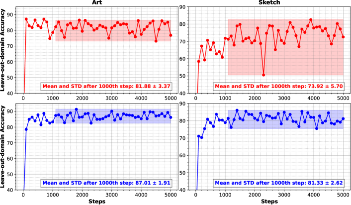
Figure 6: Accuracy (%) across training steps: Comparison between ERM (top row) vs. FDS (bottom row) in "Art" and "Sketch" domains of PACS dataset.

Stability Analysis.  In this section, we demonstrate the performance of our model across different stages of training within two domains of the PACS dataset, depicted in Figure 6. It is important to note that these test accuracies were not used in the selection of the best-performing model mentioned in earlier sections and all of our experiments follow leave-one-out settings suggested by DomainBed. The results indicate that our model achieves higher stability and better mean accuracy with lower standard deviation compared to the ERM trained on original data. Note that we cannot plot the figures for SWAD since it is a WA of ERM and does not have individual training curves. These results demonstrate the robustness and stability of our model during training, which is crucial for domain generalization algorithms.

7 Conclusion

This work presented FDS, a domain generalization (DG) technique that leverages diffusion models for domain mixing, generating a diverse set of images to bridge the domain gap between source domains distribution. We also proposed an entropy-based filtering strategy enriches the pseudo-novel generated set with images that test the limits of classifiers trained on original data, thereby boosting generalization. Our extensive experiments across multiple benchmarks demonstrate that our method not only surpasses existing DG techniques but also sets new records for accuracy. Our analysis indicate that our approach contributes to more stable training processes when confronted with domain shifts and serves effectively as a regularization method in in-domain contexts. Notably, our technique consistently enhances performance across diverse scenarios, from realistic photos to sketches. Moreover, while we exploited our trained diffusion model for covering the domain gap, more sophisticated techniques could be considered. For instance, future work could investigate the idea of generating images by extrapolate in domain space to explore pseudo-novel distributions.

FDS: Feedback-guided Domain Synthesis with Multi-Source Conditional Diffusion Models for Domain Generalization - Supplementary Material

Appendix A Implementation

Our proposed FDS method is built using the Python language and the PyTorch framework. We utlized four NVIDIA A100 GPUs for all our experiments. For initializing our models, we utilize the original Stable Diffusion version 1.5 as our initial weight  [34]. The key hyperparameter configurations employed for training these diffusion models and generating new domains are detailed in Tables 8 and 8, respectively.

Furthermore, for classifier training, we adhere to the methodologies and parameter settings described by Cha et al. [24], ensuring consistency and reproducibility in our experimental setup. The original implementation and instructions for reproducing our results are accessible via our GitHub repository.

Appendix B Additional Ablation

Selection/Filtering. In this section, we provide visual examples to show the efficacy of our synthetic sample selection and filtering mechanism. As mentioned in the method section, this mechanism is intricately designed to scrutinize the generated images through two lenses: the alignment of the predicted class with the intended label, and the entropy indicating the prediction’s uncertainty.

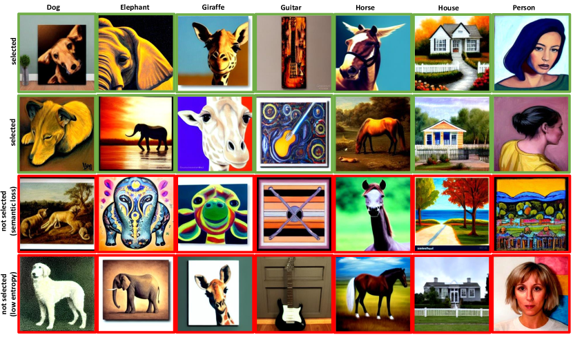
Figure 7: Synthetic images from interpolating between “art” and “photo” domains of PACS, with selected images showcasing a blend of artistic and realistic features (top two rows) and non-selected images (bottom rows) due to class mismatches and low entropy.

The Figures 7, 8, 9 showcase a set of images generated from interpolations between two domains. Specifically, the diffusion model is trained on “art”, “sketch”, and “photo” of the PACS dataset, and the selected images, demonstrated in the first two rows, exemplify successful blends of domain characteristics, embodying a balanced mixture that enriches the training data with novel, domain-bridging examples. These images were chosen based on their ability to meet our criteria: correct class prediction aligned with high entropy scores. The third and fourth rows highlight the filtering aspect of our mechanism, displaying images not selected due to class mismatches and low entropy, respectively. This visual demonstration underlines the pivotal role of our selection/filtering process in refining the synthetic dataset, ensuring only the most challenging and domain-representative samples are utilized for model training. Through this approach, we aim to significantly bolster the model’s capacity to generalize across diverse visual domains.

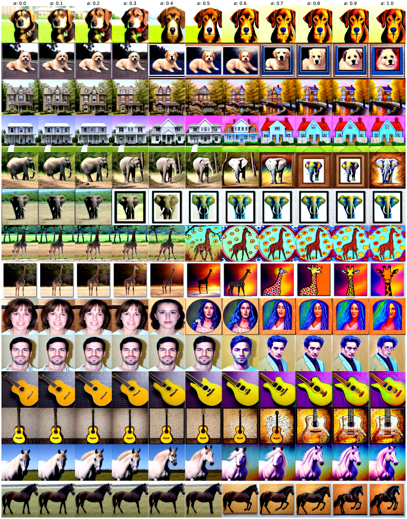
Figure 10: Inter-domain Transition from “photo” to “art”. This sequence illustrates how varying $\alpha$ from 0.0 (purely photorealistic images) to 1.0 (purely artistic representations) enables the model to seamlessly blend photographic realism with artistic expression, demonstrating a smooth progression from real-world imagery to stylized art.

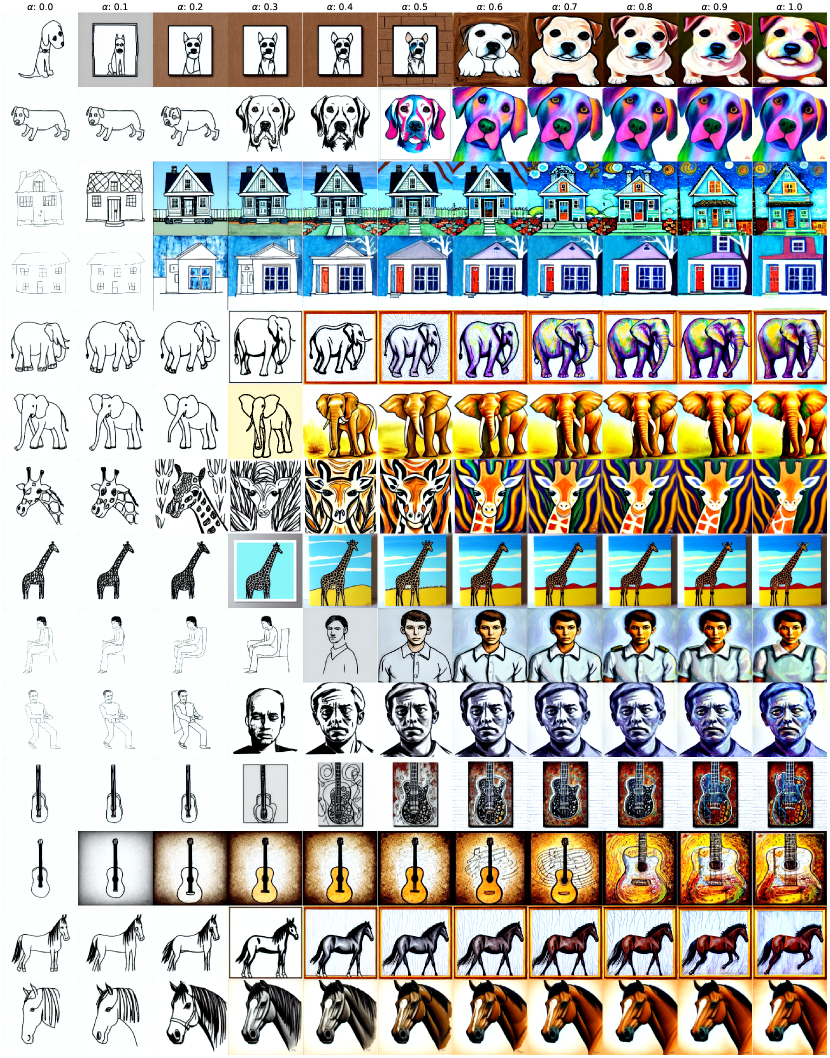
Figure 11: Inter-domain Transition from “sketch” to “art”. Displayed here is the transformation that occurs as $\alpha$ is adjusted, beginning with 0.0 (pure sketches) and moving towards 1.0 (fully art-inspired images). The model effectively infuses basic sketches with complex textures and colors, transitioning from minimalistic line art to detailed and vibrant artistic images.

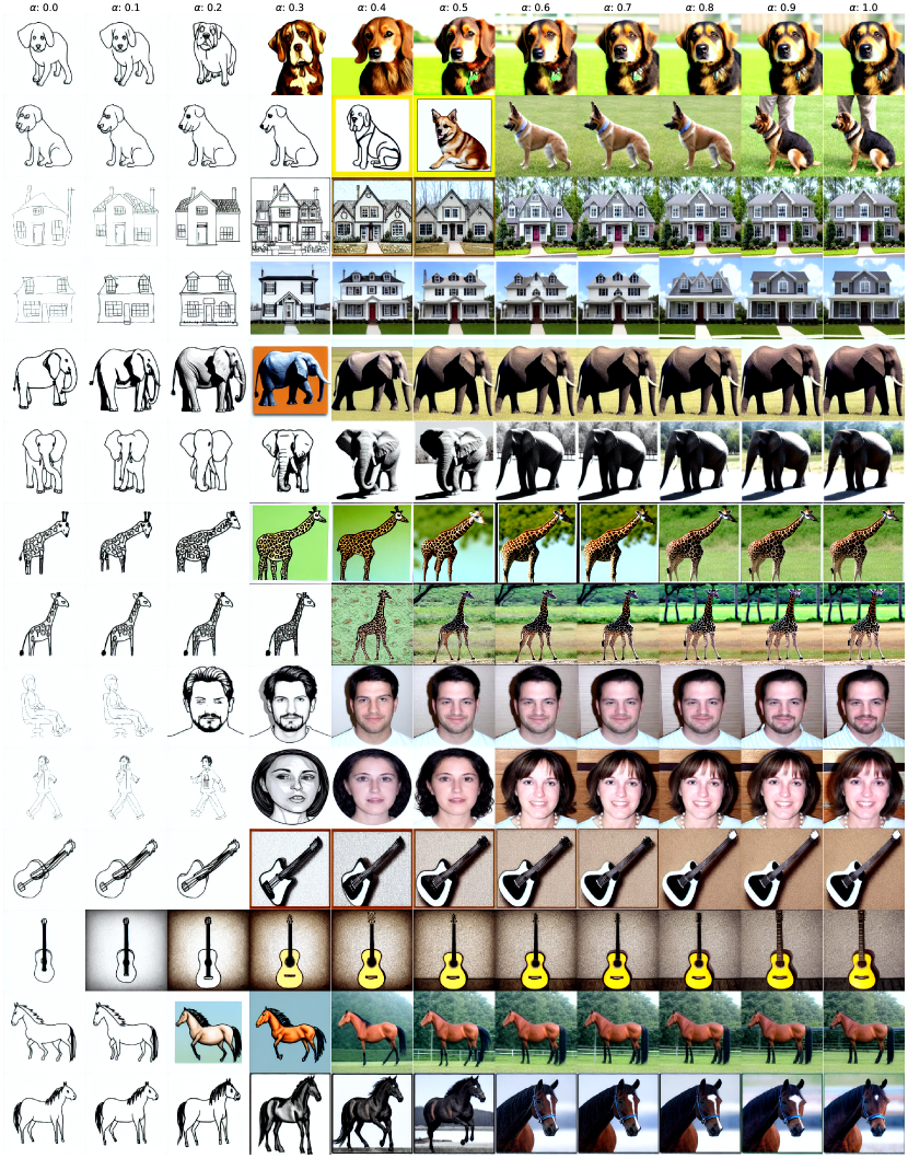
Figure 12: Inter-domain Transition from “sketch” to “photo”. This figure demonstrates the capability of the model to morph sketches into photorealistic images by altering $\alpha$ from 0.0 (entirely sketch-based) to 1.0 (completely photorealistic). The transition highlights the model’s proficiency in enriching simple outlines with lifelike details and textures, bridging the gap between abstract sketches and reality.

Inter-domain Transition. In this section, we demonstrate the model’s ability to navigate between distinct visual domains, a capability enabled by adjusting the mix coefficient $\alpha$. Trained on multiple source domains, our model can generate images that blend the unique attributes of each source domain. By varying $\alpha$ from 0.0 to 1.0, we enable smooth transitions between two source domains, where $\alpha=0.0$ and $\alpha=1.0$ correspond to generating pure images of the first and second domain, respectively. As an example, we illustrated this ability for our model trained on the PACS sources’ “art”, “sketch”, and “photo”. These domain transitions are illustrated in the figures, showcasing transitions from “photo” to “art” domain in Figure 10, “sketch” to “art” domain in Figure 11, and “sketch” to “photo” domain in Figure 12, respectively. The examples provided highlight the effectiveness of our interpolation method in producing images that incorporate the distinctive features of the mixed domains, thus affirming the model’s capability to generate novel and coherent visual content that bridges the attributes of its training domains. Note that in all of our generation experiments, we constrained $\alpha$ to the range of 0.3 to 0.7 to ensure the generated images optimally embody the characteristics of the two mixing domains, as detailed in Table 8.

Table 7: Hyperparameter Configuration for Training Diffusion Models.

Config	Value
Number of GPUs	4
Learning rate	1e-4
Learning rate scheduler	LambdaLinear
Batch size	96 (24 per GPU)
Precision	FP16
Max training steps	10000
Denosing timesteps	1000
Sampler	DDPM [33]
Autoencoder input size	256 x 256 x 3
Latent diffusion input size	32 x 32 x 4

Table 8: Hyperparameter Configuration for Generating New Domains.

Config	Value
Sampler	DDIM [35]
Denosing timesteps	50
Classifier-free guidance (CFG)	Randomly from [5, 6]
Mix coefficient $\alpha$	Randomly from [0.3, 0.7]
Mix timestep $T$	Randomly from [20, 45]
Generated images (PACS)	32k per class
Generated images (VLCS)	32k per class
Generated images (OfficeHome)	16k per class

Number of Generated Domains The impact of varying the number of generated domains on model performance was rigorously evaluated, as summarized in Table 9. This analysis aimed to understand how different combinations of augmented domains influence the overall accuracy across various dataset domains such as Art, Cartoon, Photo, and Sketch. By integrating diverse domain combinations, identified by IDs (as defined in Table 10), we observed improvement gain when we add more generated domain of different combinations. Notably, all possible combinations of augmented domains (3 new domains for PACS, VLCS and OfficeHome) were utilized as the final method, leveraging the full spectrum of available data domains.

Table 9: Analysis of the impact of utilizing different numbers/combinations of generated domains on final model performance across the PACS dataset domains (Leave-one-out accuracy). For definitions of each augmented domain (ID0, ID1, ID2), see Table 10.

Method Augmented Domains Accuracy (%) Art Cartoon Photo Sketch Avg. SWAD (reproduced) — 89.49 $\pm$0.2 83.65 $\pm$0.4 97.25 $\pm$0.2 82.06 $\pm$1.0 88.11 $\pm$0.45 SWAD + FPS ID0 91.03 $\pm$0.5 83.87 $\pm$0.6 97.75 $\pm$0.3 85.77 $\pm$0.4 89.61 $\pm$0.30 SWAD + FPS ID1 91.01 $\pm$0.6 85.06 $\pm$1.3 97.90 $\pm$0.3 83.64 $\pm$0.4 89.40 $\pm$0.65 SWAD + FPS ID2 91.46 $\pm$0.3 85.22 $\pm$0.8 97.88 $\pm$0.2 84.27 $\pm$0.3 89.71 $\pm$0.40 SWAD + FPS ID0 + ID1 91.52 $\pm$0.0 85.87 $\pm$0.7 98.03 $\pm$0.3 85.70 $\pm$1.0 90.28 $\pm$0.50 SWAD + FPS ID1 + ID2 91.62 $\pm$0.8 85.57 $\pm$0.4 98.20 $\pm$0.3 83.88 $\pm$0.6 89.82 $\pm$0.53 SWAD + FPS ID0 + ID2 91.52 $\pm$0.1 84.54 $\pm$0.5 98.28 $\pm$0.1 86.45 $\pm$0.8 90.20 $\pm$0.38 SWAD + FPS ID0 + ID1 + ID2 91.80 $\pm$0.3 86.03 $\pm$0.8 98.05 $\pm$0.2 86.11 $\pm$0.1 90.50 $\pm$0.35

Table 10: Explanation of augmented domains ID definitions for each target domain of PACS dataset.

Augmented Domains Art Cartoon Photo Sketch ID0 Cartoon + Photo Art + Photo Art + Cartoon Art + Cartoon ID1 Cartoon + Sketch Art + Sketch Art + Sketch Art + Photo ID2 Photo + Sketch Photo + Sketch Cartoon + Sketch Cartoon + Photo

Appendix C Oracle Results

In addition to leave-one-out setting, where the validation set is selected from the training domains, some studies also report the results of oracle (test-domain validation set). This can be particularly useful for understanding the potential of a method when domain knowledge is available. In this section, we compare our method (FDS+ERM) with the state-of-the-art results, as shown in Table 11. It is important to note that no Weight Averaging (WA) methods reported their oracle results within the DomainBed framework for a fair comparison. Therefore, we only train and report our ERM results here. Our proposed method, FDS+ERM, demonstrates superior performance across multiple benchmarks. Specifically, it achieves an average accuracy of 81.2%, outperforming all other methods. On the PACS dataset, FDS+ERM attains the highest accuracy of 89.7%, with significant improvements in the VLCS and OfficeHome datasets as well, achieving accuracies of 82.0% and 71.8% respectively. In addition to leave-one-out setting, these results also highlight the effectiveness of our approach in enhancing the performance under the oracle setting.

Table 11: Oracle (test-domain validation set) accuracy (%) results on the PACS, VLCS, and OfficeHome benchmarks. "Aug." indicates whether advanced augmentation or domain mixing techniques are used. The best results and second-best results are highlighted.

Method Aug. PACS VLCS OfficeHome  Avg. Standard Methods ERM (baseline) [44] ✗ 86.7 $\pm$0.3 77.6 $\pm$0.3 66.4 $\pm$0.5 76.9 ERM (reproduced) ✗ 86.6 $\pm$0.8 79.8 $\pm$0.4 68.4 $\pm$0.3 78.3 IRM [60] ✗ 84.5 $\pm$1.1 76.9 $\pm$0.6 63.0 $\pm$2.7 74.8 GroupDRO [47] ✗ 87.1 $\pm$0.1 77.4 $\pm$0.5 66.2 $\pm$0.6 76.9 Mixup [61] ✓ 86.8 $\pm$0.3 78.1 $\pm$0.3 68.0 $\pm$0.2 77.6 CORAL [62] ✗ 87.1 $\pm$0.5 77.7 $\pm$0.2 68.4 $\pm$0.2 77.7 MMD [63] ✗ 87.2 $\pm$0.1 77.9 $\pm$0.1 66.2 $\pm$0.3 77.1 DANN [64] ✗ 85.2 $\pm$0.2 79.7 $\pm$0.5 65.3 $\pm$0.8 76.7 SagNet [65] ✓ 86.4 $\pm$0.4 77.6 $\pm$0.1 67.5 $\pm$0.2 77.2 RSC [23] ✓ 86.2 $\pm$0.5 — 66.5 $\pm$0.6 — SelfReg [41] ✓ 86.7 $\pm$0.8 78.2 $\pm$0.1 68.1 $\pm$0.3 77.7 Fishr [73] ✗ 85.8 $\pm$0.6 78.2 $\pm$0.2 66.0 $\pm$2.9 76.7 CDGA [55] ✓ 89.6 $\pm$0.3 80.9 $\pm$0.1 68.8 $\pm$0.3 79.3 ERM + FDS (ours) ✓ 89.7 $\pm$0.8 82.0 $\pm$0.1 71.8 $\pm$0.9 81.2

Appendix D Detailed Results

Here we present the comprehensive tables containing all the detailed information that was summarized in the main paper. The leave-one-out performance (train-domain validation set) across different domains of PACS, VLCS, and OfficeHome datasets are detailed in the tables 12, 13, and 14, respectively. Additionally, the oracle (test-domain validation set) accuracy results for the PACS, VLCS, and OfficeHome benchmarks are detailed in Table 15, 16, and 17, respectively.

Table 12: Leave-one-out accuracy (%) results on the PACS dataset. "Aug." indicates whether advanced augmentation or domain mixing techniques are used. The best results and second-best results are highlighted.

Method Aug. Target Domains Art Cartoon Photo Sketch Avg. Standard Methods ERM (baseline) [44] ✗ 84.7 $\pm$0.4 80.8 $\pm$0.6 97.2 $\pm$0.3 79.3 $\pm$1.0 85.5 $\pm$0.2 ERM (reproduced) ✗ 86.9 $\pm$0.6 80.2 $\pm$0.7 96.6 $\pm$0.4 74.5 $\pm$2.9 84.3 $\pm$1.1 IRM [60] ✗ 84.8 $\pm$1.3 76.4 $\pm$1.1 96.7 $\pm$0.6 76.1 $\pm$1.0 83.5 $\pm$0.8 GroupDRO [47] ✗ 83.5 $\pm$0.9 79.1 $\pm$0.6 96.7 $\pm$0.3 78.3 $\pm$2.0 84.4 $\pm$0.8 Mixup [61] ✓ 86.1 $\pm$0.5 78.9 $\pm$0.8 97.6 $\pm$0.1 75.8 $\pm$1.8 84.6 $\pm$0.6 CORAL [62] ✗ 88.3 $\pm$0.2 80.0 $\pm$0.5 97.5 $\pm$0.3 78.8 $\pm$1.3 86.2 $\pm$0.3 MMD [63] ✗ 86.1 $\pm$1.4 79.4 $\pm$0.9 96.6 $\pm$0.2 76.5 $\pm$0.5 84.6 $\pm$0.5 DANN [64] ✗ 86.4 $\pm$0.8 77.4 $\pm$0.8 97.3 $\pm$0.4 73.5 $\pm$2.3 83.6 $\pm$0.4 MLDG [15] ✗ 85.5 $\pm$1.4 80.1 $\pm$1.7 97.4 $\pm$0.3 76.6 $\pm$1.1 84.9 $\pm$1.1 VREx [74] ✗ 86.0 $\pm$1.6 79.1 $\pm$0.6 96.9 $\pm$0.5 77.7 $\pm$1.7 84.9 $\pm$1.1 ARM [75] ✗ 86.8 $\pm$0.6 76.8 $\pm$0.5 97.4 $\pm$0.3 79.3 $\pm$1.2 85.1 $\pm$0.6 SagNet [65] ✓ 87.4 $\pm$1.0 80.7 $\pm$0.6 97.1 $\pm$0.1 80.0 $\pm$0.4 86.3 $\pm$0.2 RSC [23] ✓ 85.4 $\pm$0.8 79.7 $\pm$1.8 97.6 $\pm$0.3 78.2 $\pm$1.2 85.2 $\pm$0.9 Mixstyle [20] ✓ 86.8 $\pm$0.5 79.0 $\pm$1.4 96.6 $\pm$0.1 78.5 $\pm$2.3 85.2 $\pm$0.3 mDSDI [66] ✗ 87.7 $\pm$0.4 80.4 $\pm$0.7 98.1 $\pm$0.3 78.4 $\pm$1.2 86.2 $\pm$0.2 SelfReg [41] ✓ 87.9 $\pm$1.0 79.4 $\pm$1.4 96.8 $\pm$0.7 78.3 $\pm$1.2 85.6 $\pm$0.4 Fishr [73] ✗ 88.4 $\pm$0.2 78.7 $\pm$0.7 97.0 $\pm$0.1 77.8 $\pm$2.0 85.5 $\pm$0.5 DCAug [59] ✓ 88.5 $\pm$0.8 78.8 $\pm$1.5 96.3 $\pm$0.1 80.8 $\pm$0.5 86.1 $\pm$0.7 CDGA [55] ✓ 89.1 $\pm$1.0 82.5 $\pm$0.5 97.4 $\pm$0.2 84.8 $\pm$0.9 88.5 $\pm$0.5 ERM + FDS (ours) ✓ 90.7 $\pm$0.9 84.2 $\pm$0.6 97.2 $\pm$0.1 83.0 $\pm$0.4 88.8 $\pm$0.1 WA Methods SWAD (baseline) [24] ✗ 89.3 $\pm$0.2 83.4 $\pm$0.6 97.3 $\pm$0.3 82.5 $\pm$0.5 88.1 $\pm$0.1 SWAD (reproduced) ✗ 89.5 $\pm$0.2 83.7 $\pm$0.4 97.3 $\pm$0.2 82.1 $\pm$0.1 88.1 $\pm$0.4 SelfReg SWA [41] ✓ 85.9 $\pm$0.6 81.9 $\pm$0.4 96.8 $\pm$0.1 81.4 $\pm$0.6 86.5 $\pm$0.3 DNA [67] ✗ 89.8 $\pm$0.2 83.4 $\pm$0.4 97.7 $\pm$0.1 82.6 $\pm$0.2 88.4 $\pm$0.1 DiWA [68] ✓ 90.1 $\pm$0.6 83.3 $\pm$0.6 98.2 $\pm$0.1 83.4 $\pm$0.4 88.8 $\pm$0.4 TeachDCAug [59] ✓ 89.6 $\pm$0.0 81.8 $\pm$0.5 97.7 $\pm$0.0 84.5 $\pm$0.2 88.4 $\pm$0.2 SWAD + FDS (ours) ✓ 91.8 $\pm$0.3 86.0 $\pm$0.8 98.1 $\pm$0.2 86.1 $\pm$0.1 90.5 $\pm$0.3

Table 13: Leave-one-out accuracy (%) results on the VLCS dataset. "Aug." indicates whether advanced augmentation or domain mixing techniques are used. The best results and second-best results are highlighted.

Method Aug. Target Domains Caltech101 LabelMe SUN09 VOC2007 Avg. Standard Methods ERM (baseline) [44] ✗ 97.7 $\pm$0.4 64.3 $\pm$0.9 73.4 $\pm$0.5 74.6 $\pm$1.3 77.5 $\pm$0.4 ERM (reproduced) ✗ 96.9 $\pm$1.4 64.1 $\pm$1.4 71.1 $\pm$1.5 72.8 $\pm$0.9 76.2 $\pm$1.1 IRM [60] ✗ 98.6 $\pm$0.1 64.9 $\pm$0.9 73.4 $\pm$0.6 77.3 $\pm$0.9 78.5 $\pm$0.5 GroupDRO [47] ✗ 97.3 $\pm$0.3 63.4 $\pm$0.9 69.5 $\pm$0.8 76.7 $\pm$0.7 76.7 $\pm$0.6 Mixup [61] ✓ 98.3 $\pm$0.6 64.8 $\pm$1.0 72.1 $\pm$0.5 74.3 $\pm$0.8 77.4 $\pm$0.6 CORAL [62] ✗ 98.3 $\pm$0.1 66.1 $\pm$1.2 73.4 $\pm$0.3 77.5 $\pm$1.2 78.8 $\pm$0.6 MMD [63] ✗ 97.7 $\pm$0.1 64.0 $\pm$1.1 72.8 $\pm$0.2 75.3 $\pm$3.3 77.5 $\pm$0.9 DANN [64] ✗ 99.0 $\pm$0.3 65.1 $\pm$1.4 73.1 $\pm$0.3 77.2 $\pm$0.6 78.6 $\pm$0.4 MLDG [15] ✗ 97.4 $\pm$0.2 65.2 $\pm$0.7 71.0 $\pm$1.4 75.3 $\pm$1.0 77.2 $\pm$0.8 VREx [74] ✗ 98.4 $\pm$0.3 64.4 $\pm$1.4 74.1 $\pm$0.4 76.2 $\pm$1.3 78.3 $\pm$0.8 ARM [75] ✗ 98.7 $\pm$0.2 63.6 $\pm$0.7 71.3 $\pm$1.2 76.7 $\pm$0.6 77.6 $\pm$0.6 SagNet [65] ✓ 97.9 $\pm$0.4 64.5 $\pm$0.5 71.4 $\pm$1.3 77.5 $\pm$0.5 77.8 $\pm$0.5 RSC [23] ✓ 97.9 $\pm$0.1 62.5 $\pm$0.7 72.3 $\pm$1.2 75.6 $\pm$0.8 77.1 $\pm$0.5 Mixstyle [20] ✓ 98.6 $\pm$0.3 64.5 $\pm$1.1 72.6 $\pm$0.5 75.7 $\pm$1.7 77.9 $\pm$0.5 mDSDI [66] ✗ 97.6 $\pm$0.1 66.4 $\pm$0.4 74.0 $\pm$0.6 77.8 $\pm$0.7 79.0 $\pm$0.3 SelfReg [41] ✓ 96.7 $\pm$0.4 65.2 $\pm$1.2 73.1 $\pm$1.3 76.2 $\pm$0.7 77.8 $\pm$0.9 Fishr [73] ✗ 98.9 $\pm$0.3 64.0 $\pm$0.5 71.5 $\pm$0.2 76.8 $\pm$0.7 77.8 $\pm$0.5 DCAug [59] ✓ 98.3 $\pm$0.1 64.2 $\pm$0.4 74.4 $\pm$0.6 77.5 $\pm$0.3 78.6 $\pm$0.5 CDGA [55] ✓ 96.3 $\pm$0.7 75.7 $\pm$1.0 72.8 $\pm$1.3 73.7 $\pm$1.3 79.6 $\pm$0.9 ERM + FDS (ours) ✓ 98.8 $\pm$0.3 65.6 $\pm$0.9 75.5 $\pm$0.9 79.3 $\pm$1.8 79.8 $\pm$0.5 WA Methods SWAD (baseline) [24] ✗ 98.8 $\pm$0.1 63.3 $\pm$0.3 75.3 $\pm$0.5 79.2 $\pm$0.6 79.1 $\pm$0.1 SWAD (reproduced) ✗ 98.7 $\pm$0.2 63.9 $\pm$0.3 74.3 $\pm$1.1 78.6 $\pm$0.6 78.9 $\pm$0.5 SelfReg SWA [41] ✓ 97.4 $\pm$0.4 63.5 $\pm$0.3 72.6 $\pm$0.1 76.7 $\pm$0.7 77.5 $\pm$0.0 DNA [67] ✗ 98.8 $\pm$0.1 63.6 $\pm$0.2 74.1 $\pm$0.1 79.5 $\pm$0.4 79.0 $\pm$0.5 DiWA [68] ✓ 98.4 $\pm$0.1 63.4 $\pm$0.1 75.5 $\pm$0.3 78.9 $\pm$0.6 79.1 $\pm$0.2 TeachDCAug [59] ✓ 98.5 $\pm$0.1 63.7 $\pm$0.3 75.6 $\pm$0.5 77.0 $\pm$0.7 78.7 $\pm$0.5 SWAD + FDS (ours) ✓ 99.5 $\pm$0.2 62.9 $\pm$0.2 76.9 $\pm$0.4 79.6 $\pm$1.3 79.7 $\pm$0.5

Table 14: Leave-one-out accuracy (%) results on the OfficeHome dataset. "Aug." indicates whether advanced augmentation or domain mixing techniques are used. The best results and second-best results are highlighted.

Method Aug. Target Domains Art Clipart Product Real World Avg. Standard Methods ERM (baseline) [44] ✗ 61.3 $\pm$0.7 52.4 $\pm$0.3 75.8 $\pm$0.1 76.6 $\pm$0.3 66.5 $\pm$0.3 ERM (reproduced) ✗ 59.5 $\pm$2.1 51.3 $\pm$1.3 73.8 $\pm$0.8 73.8 $\pm$0.2 64.6 $\pm$1.1 IRM [60] ✗ 58.9 $\pm$2.3 52.2 $\pm$1.6 72.1 $\pm$2.9 74.0 $\pm$2.5 64.3 $\pm$2.2 GroupDRO [47] ✗ 60.4 $\pm$0.7 52.7 $\pm$1.0 75.0 $\pm$0.7 76.0 $\pm$0.7 66.0 $\pm$0.7 Mixup [61] ✓ 62.4 $\pm$0.8 54.8 $\pm$0.6 76.9 $\pm$0.3 78.3 $\pm$0.2 68.1 $\pm$0.3 CORAL [62] ✗ 65.3 $\pm$0.4 54.4 $\pm$0.5 76.5 $\pm$0.1 78.4 $\pm$0.5 68.7 $\pm$0.3 MMD [63] ✗ 60.4 $\pm$0.2 53.3 $\pm$0.3 74.3 $\pm$0.1 77.4 $\pm$0.6 66.3 $\pm$0.1 DANN [64] ✗ 59.9 $\pm$1.3 53.0 $\pm$0.3 73.6 $\pm$0.7 76.9 $\pm$0.5 65.9 $\pm$0.6 MLDG [15] ✗ 61.5 $\pm$0.9 53.2 $\pm$0.6 75.0 $\pm$1.2 77.5 $\pm$0.4 66.8 $\pm$0.7 VREx [74] ✗ 60.7 $\pm$0.9 53.0 $\pm$0.9 75.3 $\pm$0.1 76.6 $\pm$0.5 66.4 $\pm$0.6 ARM [75] ✗ 58.9 $\pm$0.8 51.0 $\pm$0.5 74.1 $\pm$0.1 75.2 $\pm$0.3 64.8 $\pm$0.4 SagNet [65] ✓ 63.4 $\pm$0.2 54.8 $\pm$0.4 75.8 $\pm$0.4 78.3 $\pm$0.3 68.1 $\pm$0.1 RSC [23] ✓ 60.7 $\pm$1.4 51.4 $\pm$0.3 74.8 $\pm$1.1 75.1 $\pm$1.3 65.5 $\pm$0.9 Mixstyle [20] ✓ 51.1 $\pm$0.3 53.2 $\pm$0.4 68.2 $\pm$0.7 69.2 $\pm$0.6 60.4 $\pm$0.3 mDSDI [66] ✗ 68.1 $\pm$0.3 52.1 $\pm$0.4 76.0 $\pm$0.2 80.4 $\pm$0.2 69.2 $\pm$0.4 SelfReg [41] ✓ 63.6 $\pm$1.4 53.1 $\pm$1.0 76.9 $\pm$0.4 78.1 $\pm$0.4 67.9 $\pm$0.7 Fishr [73] ✗ 62.4 $\pm$0.5 54.4 $\pm$0.4 76.2 $\pm$0.5 78.3 $\pm$0.1 67.8 $\pm$0.5 DCAug [59] ✓ 61.8 $\pm$0.6 55.4 $\pm$0.6 77.1 $\pm$0.3 78.9 $\pm$0.3 68.3 $\pm$0.4 CDGA [55] ✓ 60.1 $\pm$1.4 54.2 $\pm$0.5 78.2 $\pm$0.6 80.4 $\pm$0.1 68.2 $\pm$0.6 ERM + FDS (ours) ✓ 64.6 $\pm$0.2 57.7 $\pm$0.1 80.2 $\pm$0.5 82.0 $\pm$0.4 71.1 $\pm$0.1 WA Methods SWAD (baseline) [24] ✗ 66.1 $\pm$0.4 57.7 $\pm$0.4 78.4 $\pm$0.1 80.2 $\pm$0.2 70.6 $\pm$0.2 SWAD (reproduced) ✗ 65.9 $\pm$0.9 56.8 $\pm$0.4 78.8 $\pm$0.3 80.0 $\pm$0.2 70.3 $\pm$0.4 SelfReg SWA [41] ✓ 64.9 $\pm$0.8 55.4 $\pm$0.6 78.4 $\pm$0.2 78.8 $\pm$0.1 69.4 $\pm$0.2 DNA [67] ✗ 67.7 $\pm$0.2 57.7 $\pm$0.3 78.9 $\pm$0.2 80.5 $\pm$0.2 71.2 $\pm$0.1 DiWA [68] ✓ 67.3 $\pm$0.2 57.9 $\pm$0.2 79.0 $\pm$0.2 79.9 $\pm$0.1 71.0 $\pm$0.1 TeachDCAug [59] ✓ 66.2 $\pm$0.2 57.0 $\pm$0.3 78.3 $\pm$0.1 80.1 $\pm$0.0 70.4 $\pm$0.2 SWAD + FDS (ours) ✓ 67.3 $\pm$0.8 60.5 $\pm$0.5 82.6 $\pm$0.1 83.6 $\pm$0.3 73.5 $\pm$0.4

Table 15: Oracle (test-domain validation set) accuracy (%) results on the PACS dataset. "Aug." indicates whether advanced augmentation or domain mixing techniques are used. The best results and second-best results are highlighted.

Method Aug. Target Domains Art Cartoon Photo Sketch Avg. Standard Methods ERM (baseline) [44] ✗ 86.5 $\pm$1.0 81.3 $\pm$0.6 96.2 $\pm$0.3 82.7 $\pm$1.1 86.7 $\pm$0.8 ERM (reproduced) ✗ 88.6 $\pm$0.9 80.9 $\pm$1.9 98.4 $\pm$0.4 78.4 $\pm$1.2 86.6 $\pm$1.0 IRM ✗ 84.2 $\pm$0.9 79.7 $\pm$1.5 95.9 $\pm$0.4 78.3 $\pm$2.1 84.5 $\pm$1.2 GroupDRO ✗ 87.5 $\pm$0.5 82.9 $\pm$0.6 97.1 $\pm$0.3 81.1 $\pm$1.2 87.2 $\pm$0.7 Mixup ✓ 87.5 $\pm$0.4 81.6 $\pm$0.7 97.4 $\pm$0.2 80.8 $\pm$0.9 86.8 $\pm$0.6 CORAL ✗ 86.6 $\pm$0.8 81.8 $\pm$0.9 97.1 $\pm$0.5 82.7 $\pm$0.6 87.1 $\pm$0.7 MMD ✗ 88.1 $\pm$0.8 82.6 $\pm$0.7 97.1 $\pm$0.5 81.2 $\pm$1.2 87.3 $\pm$0.8 DANN ✗ 87.0 $\pm$0.4 80.3 $\pm$0.6 96.8 $\pm$0.3 76.9 $\pm$1.1 85.3 $\pm$0.6 SagNet ✓ 87.4 $\pm$0.5 81.2 $\pm$1.2 96.3 $\pm$0.8 80.7 $\pm$1.1 86.4 $\pm$0.9 RSC ✓ 86.0 $\pm$0.7 81.8 $\pm$0.9 96.8 $\pm$0.7 80.4 $\pm$0.5 86.3 $\pm$0.7 Fishr ✗ 87.9 $\pm$0.6 80.8 $\pm$0.5 97.9 $\pm$0.4 81.1 $\pm$0.8 86.9 $\pm$0.6 SelfReg ✓ 87.9 $\pm$0.5 80.6 $\pm$1.1 97.1 $\pm$0.4 81.1 $\pm$1.3 86.7 $\pm$0.8 CDGA ✓ 89.6 $\pm$0.8 85.3 $\pm$0.7 97.3 $\pm$0.3 86.2 $\pm$0.5 89.6 $\pm$0.6 ERM + FDS (ours) ✓ 91.1 $\pm$0.3 84.9 $\pm$0.7 97.3 $\pm$0.5 85.6 $\pm$2.3 89.7 $\pm$0.8

Table 16: Oracle (test-domain validation set) accuracy (%) results on the VLCS dataset. "Aug." indicates whether advanced augmentation or domain mixing techniques are used. The best results and second-best results are highlighted.

Method Aug. Target Domains Caltech101 LabelMe SUN09 VOC2007 Avg. Standard Methods ERM (baseline) [44] ✗ 97.6 $\pm$0.3 67.9 $\pm$0.7 70.9 $\pm$0.2 74.0 $\pm$0.6 77.6 $\pm$0.5 ERM (reproduced) ✗ 98.6 $\pm$0.2 68.6 $\pm$0.7 73.6 $\pm$1.7 78.6 $\pm$1.2 79.8 $\pm$0.4 IRM ✗ 97.3 $\pm$0.2 66.7 $\pm$0.1 71.0 $\pm$2.3 72.8 $\pm$0.4 77.0 $\pm$0.8 GroupDRO ✗ 97.7 $\pm$0.2 65.9 $\pm$0.2 72.8 $\pm$0.8 73.4 $\pm$1.3 77.5 $\pm$0.6 Mixup ✓ 97.8 $\pm$0.4 67.2 $\pm$0.4 71.5 $\pm$0.2 75.7 $\pm$0.6 78.1 $\pm$0.4 CORAL ✗ 97.3 $\pm$0.2 67.5 $\pm$0.6 71.6 $\pm$0.6 74.5 $\pm$0.0 77.7 $\pm$0.4 MMD ✗ 98.8 $\pm$0.0 66.4 $\pm$0.4 70.8 $\pm$0.5 75.6 $\pm$0.4 77.9 $\pm$0.3 DANN ✗ 9.0 $\pm$0.2 66.3 $\pm$1.2 73.4 $\pm$1.4 80.1 $\pm$0.5 79.7 $\pm$0.8 SagNet ✓ 97.4 $\pm$0.3 66.4 $\pm$0.4 71.6 $\pm$0.1 75.0 $\pm$0.8 77.6 $\pm$0.4 RSC ✓ 98.0 $\pm$0.4 67.2 $\pm$0.3 70.3 $\pm$1.3 75.6 $\pm$0.4 77.8 $\pm$0.6 Fishr ✗ 97.6 $\pm$0.7 67.3 $\pm$0.5 72.2 $\pm$0.9 75.7 $\pm$0.3 78.2 $\pm$0.6 SelfReg ✓ 98.2 $\pm$0.3 63.9 $\pm$0.8 72.2 $\pm$0.1 75.5 $\pm$0.4 77.5 $\pm$0.2 CDGA ✓ 96.6 $\pm$0.7 75.5 $\pm$1.9 73.6 $\pm$1.1 77.8 $\pm$1.0 80.9 $\pm$1.2 ERM + FDS (ours) ✓ 99.5 $\pm$0.1 68.7 $\pm$0.3 77.4 $\pm$0.7 82.6 $\pm$0.1 82.0 $\pm$0.1

Table 17: Oracle (test-domain validation set) accuracy (%) results on the OfficeHome dataset. "Aug." indicates whether advanced augmentation or domain mixing techniques are used. The best results and second-best results are highlighted.

Method Aug. Target Domains Art Clipart Product Real World Avg. Standard Methods ERM (baseline) [44] ✗ 61.7 $\pm$0.7 53.4 $\pm$0.3 74.1 $\pm$0.4 76.2 $\pm$0.6 66.4 $\pm$0.5 ERM (reproduced) ✗ 64.0 $\pm$0.9 53.7 $\pm$1.1 77.1 $\pm$0.3 78.8 $\pm$0.4 68.4 $\pm$0.3 IRM ✗ 56.4 $\pm$3.2 51.2 $\pm$2.3 71.7 $\pm$2.7 72.7 $\pm$2.7 63.0 $\pm$2.7 GroupDRO ✗ 60.5 $\pm$1.6 53.1 $\pm$0.3 75.5 $\pm$0.3 75.9 $\pm$0.7 66.3 $\pm$0.7 Mixup ✓ 63.5 $\pm$0.2 54.6 $\pm$0.4 76.0 $\pm$0.3 78.0 $\pm$0.7 68.0 $\pm$0.4 CORAL ✗ 64.8 $\pm$0.8 54.1 $\pm$0.9 76.5 $\pm$0.4 78.2 $\pm$0.4 68.4 $\pm$0.6 MMD ✗ 60.4 $\pm$1.0 53.4 $\pm$0.5 74.9 $\pm$0.1 76.1 $\pm$0.7 66.2 $\pm$0.6 DANN ✗ 60.6 $\pm$1.4 51.8 $\pm$0.7 73.4 $\pm$0.5 75.5 $\pm$0.9 65.3 $\pm$0.9 SagNet ✓ 62.7 $\pm$0.5 53.6 $\pm$0.5 76.0 $\pm$0.3 77.8 $\pm$0.1 67.5 $\pm$0.4 RSC ✓ 61.7 $\pm$0.8 53.0 $\pm$0.9 74.8 $\pm$0.8 76.3 $\pm$0.5 66.5 $\pm$0.8 Fishr ✗ 63.4 $\pm$0.8 54.2 $\pm$0.3 76.4 $\pm$0.3 78.5 $\pm$0.2 68.1 $\pm$0.4 SelfReg ✓ 64.2 $\pm$0.6 53.6 $\pm$0.7 76.7 $\pm$0.3 77.9 $\pm$0.5 68.1 $\pm$0.3 CDGA ✓ 61.1 $\pm$1.1 55.9 $\pm$1.0 78.2 $\pm$0.8 79.8 $\pm$0.2 68.8 $\pm$0.8 ERM + FDS (ours) ✓ 65.3 $\pm$0.8 58.4 $\pm$0.8 81.2 $\pm$0.2 82.4 $\pm$0.6 71.8 $\pm$0.9

Figure 8: Interpolation between “art” and “sketch” in PACS highlights selected images (top rows) merging textures and outlines, and non-selected images (bottom rows) for failing selection criteria.

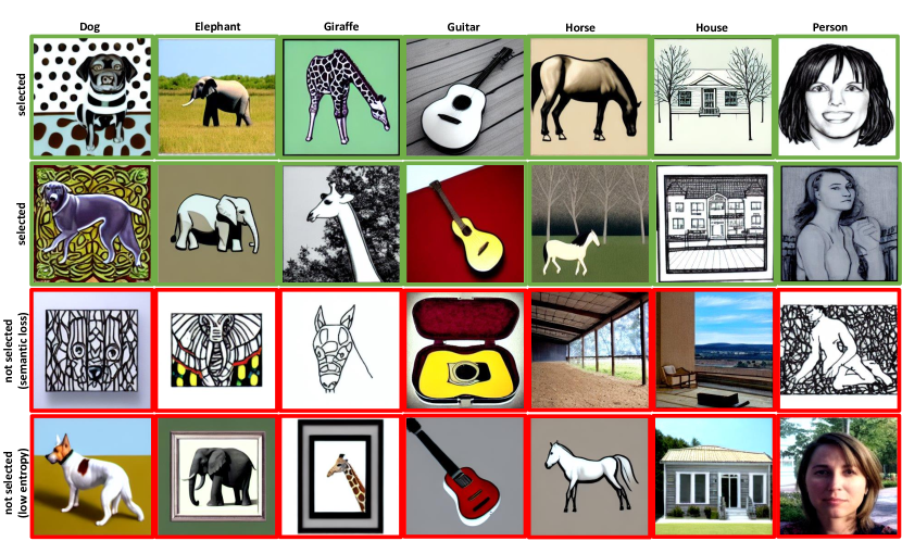
Figure 9: Results from “photo” and “sketch” domain interpolation in PACS, with selected synthetic images (top rows) and non-selected due to predictability and class misalignment (bottom rows).

References

- [1] Benjamin Recht, Rebecca Roelofs, Ludwig Schmidt, and Vaishaal Shankar. Do imagenet classifiers generalize to imagenet? In International Conference on Machine Learning, pages 5389–5400. PMLR, 2019.
- [2] Dan Hendrycks and Thomas Dietterich. Benchmarking neural network robustness to common corruptions and perturbations. arXiv preprint arXiv:1903.12261, 2019.
- [3] Zhihe Lu, Yongxin Yang, Xiatian Zhu, Cong Liu, Yi-Zhe Song, and Tao Xiang. Stochastic classifiers for unsupervised domain adaptation. In Proceedings of the IEEE/CVF Conference on Computer Vision and Pattern Recognition, pages 9111–9120, 2020.
- [4] Kuniaki Saito, Kohei Watanabe, Yoshitaka Ushiku, and Tatsuya Harada. Maximum classifier discrepancy for unsupervised domain adaptation. In Proceedings of the IEEE conference on computer vision and pattern recognition, pages 3723–3732, 2018.
- [5] Yaroslav Ganin and Victor Lempitsky. Unsupervised domain adaptation by backpropagation. In International conference on machine learning, pages 1180–1189. PMLR, 2015.
- [6] Dequan Wang, Evan Shelhamer, Shaoteng Liu, Bruno Olshausen, and Trevor Darrell. Tent: Fully test-time adaptation by entropy minimization. arXiv preprint arXiv:2006.10726, 2020.
- [7] Gustavo A Vargas Hakim, David Osowiechi, Mehrdad Noori, Milad Cheraghalikhani, Ali Bahri, Ismail Ben Ayed, and Christian Desrosiers. Clust3: Information invariant test-time training. In Proceedings of the IEEE/CVF International Conference on Computer Vision, pages 6136–6145, 2023.
- [8] David Osowiechi, Gustavo A Vargas Hakim, Mehrdad Noori, Milad Cheraghalikhani, Ismail Ben Ayed, and Christian Desrosiers. Tttflow: Unsupervised test-time training with normalizing flow. In Proceedings of the IEEE/CVF Winter Conference on Applications of Computer Vision, pages 2126–2134, 2023.
- [9] Gilles Blanchard, Gyemin Lee, and Clayton Scott. Generalizing from several related classification tasks to a new unlabeled sample. Advances in neural information processing systems, 24:2178–2186, 2011.
- [10] Kaiyang Zhou, Ziwei Liu, Yu Qiao, Tao Xiang, and Chen Change Loy. Domain generalization: A survey. IEEE Transactions on Pattern Analysis and Machine Intelligence, 2022.
- [11] Jindong Wang, Cuiling Lan, Chang Liu, Yidong Ouyang, Tao Qin, Wang Lu, Yiqiang Chen, Wenjun Zeng, and Philip Yu. Generalizing to unseen domains: A survey on domain generalization. IEEE Transactions on Knowledge and Data Engineering, 2022.
- [12] Shoubo Hu, Kun Zhang, Zhitang Chen, and Laiwan Chan. Domain generalization via multidomain discriminant analysis. In Uncertainty in Artificial Intelligence, pages 292–302. PMLR, 2020.
- [13] Divyat Mahajan, Shruti Tople, and Amit Sharma. Domain generalization using causal matching. In International Conference on Machine Learning, pages 7313–7324. PMLR, 2021.
- [14] Haoliang Li, YuFei Wang, Renjie Wan, Shiqi Wang, Tie-Qiang Li, and Alex Kot. Domain generalization for medical imaging classification with linear-dependency regularization. Advances in Neural Information Processing Systems, 33:3118–3129, 2020.
- [15] Da Li, Yongxin Yang, Yi-Zhe Song, and Timothy M Hospedales. Learning to generalize: Meta-learning for domain generalization. In Thirty-Second AAAI Conference on Artificial Intelligence, 2018.
- [16] Yogesh Balaji, Swami Sankaranarayanan, and Rama Chellappa. Metareg: Towards domain generalization using meta-regularization. Advances in neural information processing systems, 31, 2018.
- [17] Yichun Shi, Xiang Yu, Kihyuk Sohn, Manmohan Chandraker, and Anil K Jain. Towards universal representation learning for deep face recognition. In Proceedings of the IEEE/CVF Conference on Computer Vision and Pattern Recognition, pages 6817–6826, 2020.
- [18] Riccardo Volpi, Hongseok Namkoong, Ozan Sener, John C Duchi, Vittorio Murino, and Silvio Savarese. Generalizing to unseen domains via adversarial data augmentation. In Advances in Neural Information Processing Systems, pages 5334–5344, 2018.
- [19] Shiv Shankar, Vihari Piratla, Soumen Chakrabarti, Siddhartha Chaudhuri, Preethi Jyothi, and Sunita Sarawagi. Generalizing across domains via cross-gradient training. In International Conference on Learning Representations, 2018.
- [20] Kaiyang Zhou, Yongxin Yang, Yu Qiao, and Tao Xiang. Domain generalization with mixstyle. In International Conference on Learning Representations, 2021.
- [21] Fabio M Carlucci, Antonio D’Innocente, Silvia Bucci, Barbara Caputo, and Tatiana Tommasi. Domain generalization by solving jigsaw puzzles. In Proceedings of the IEEE Conference on Computer Vision and Pattern Recognition, pages 2229–2238, 2019.
- [22] Isabela Albuquerque, Nikhil Naik, Junnan Li, Nitish Keskar, and Richard Socher. Improving out-of-distribution generalization via multi-task self-supervised pretraining. arXiv preprint arXiv:2003.13525, 2020.
- [23] Zeyi Huang, Haohan Wang, Eric P Xing, and Dong Huang. Self-challenging improves cross-domain generalization. In European Conference on Computer Vision, pages 124–140. Springer, 2020.
- [24] Junbum Cha, Sanghyuk Chun, Kyungjae Lee, Han-Cheol Cho, Seunghyun Park, Yunsung Lee, and Sungrae Park. Swad: Domain generalization by seeking flat minima. Advances in Neural Information Processing Systems, 34, 2021.
- [25] Ling Zhang, Xiaosong Wang, Dong Yang, Thomas Sanford, Stephanie Harmon, Baris Turkbey, Bradford J Wood, Holger Roth, Andriy Myronenko, Daguang Xu, et al. Generalizing deep learning for medical image segmentation to unseen domains via deep stacked transformation. IEEE transactions on medical imaging, 39(7):2531–2540, 2020.
- [26] Nathan Somavarapu, Chih-Yao Ma, and Zsolt Kira. Frustratingly simple domain generalization via image stylization. arXiv preprint arXiv:2006.11207, 2020.
- [27] Francesco Cappio Borlino, Antonio D’Innocente, and Tatiana Tommasi. Rethinking domain generalization baselines. In 2020 25th International Conference on Pattern Recognition (ICPR), pages 9227–9233. IEEE, 2021.
- [28] Kaiyang Zhou, Yongxin Yang, Timothy Hospedales, and Tao Xiang. Deep domain-adversarial image generation for domain generalisation. In Proceedings of the AAAI Conference on Artificial Intelligence, volume 34, pages 13025–13032, 2020.
- [29] Kaiyang Zhou, Yongxin Yang, Timothy Hospedales, and Tao Xiang. Learning to generate novel domains for domain generalization. In Computer Vision–ECCV 2020: 16th European Conference, Glasgow, UK, August 23–28, 2020, Proceedings, Part XVI 16, pages 561–578. Springer, 2020.
- [30] Fabio Maria Carlucci, Paolo Russo, Tatiana Tommasi, and Barbara Caputo. Hallucinating agnostic images to generalize across domains. In 2019 IEEE/CVF International Conference on Computer Vision Workshop (ICCVW), pages 3227–3234. IEEE, 2019.
- [31] Mehrdad Noori, Milad Cheraghalikhani, Ali Bahri, Gustavo A Vargas Hakim, David Osowiechi, Ismail Ben Ayed, and Christian Desrosiers. Tfs-vit: Token-level feature stylization for domain generalization. Pattern Recognition, 149:110213, 2024.
- [32] Prafulla Dhariwal and Alexander Nichol. Diffusion models beat gans on image synthesis. Advances in neural information processing systems, 34:8780–8794, 2021.
- [33] Jonathan Ho, Ajay Jain, and Pieter Abbeel. Denoising diffusion probabilistic models. Advances in neural information processing systems, 33:6840–6851, 2020.
- [34] Robin Rombach, Andreas Blattmann, Dominik Lorenz, Patrick Esser, and Björn Ommer. High-resolution image synthesis with latent diffusion models. In Proceedings of the IEEE/CVF conference on computer vision and pattern recognition, pages 10684–10695, 2022.
- [35] Jiaming Song, Chenlin Meng, and Stefano Ermon. Denoising diffusion implicit models. arXiv preprint arXiv:2010.02502, 2020.
- [36] Xingchao Peng, Qinxun Bai, Xide Xia, Zijun Huang, Kate Saenko, and Bo Wang. Moment matching for multi-source domain adaptation. In Proceedings of the IEEE International Conference on Computer Vision, pages 1406–1415, 2019.
- [37] Ya Li, Xinmei Tian, Mingming Gong, Yajing Liu, Tongliang Liu, Kun Zhang, and Dacheng Tao. Deep domain generalization via conditional invariant adversarial networks. In Proceedings of the European Conference on Computer Vision (ECCV), pages 624–639, 2018.
- [38] Massimiliano Mancini, Samuel Rota Bulò, Barbara Caputo, and Elisa Ricci. Best sources forward: domain generalization through source-specific nets. In 2018 25th IEEE International Conference on Image Processing (ICIP), pages 1353–1357. IEEE, 2018.
- [39] Shujun Wang, Lequan Yu, Caizi Li, Chi-Wing Fu, and Pheng-Ann Heng. Learning from extrinsic and intrinsic supervisions for domain generalization. In European Conference on Computer Vision, pages 159–176. Springer, 2020.
- [40] Muhammad Ghifary, W Bastiaan Kleijn, Mengjie Zhang, and David Balduzzi. Domain generalization for object recognition with multi-task autoencoders. In Proceedings of the IEEE international conference on computer vision, pages 2551–2559, 2015.
- [41] Daehee Kim, Youngjun Yoo, Seunghyun Park, Jinkyu Kim, and Jaekoo Lee. Selfreg: Self-supervised contrastive regularization for domain generalization. In Proceedings of the IEEE/CVF International Conference on Computer Vision, pages 9619–9628, 2021.
- [42] Da Li, Yongxin Yang, Yi-Zhe Song, and Timothy M Hospedales. Deeper, broader and artier domain generalization. In Proceedings of the IEEE international conference on computer vision, pages 5542–5550, 2017.
- [43] Prithvijit Chattopadhyay, Yogesh Balaji, and Judy Hoffman. Learning to balance specificity and invariance for in and out of domain generalization. In Computer Vision–ECCV 2020: 16th European Conference, Glasgow, UK, August 23–28, 2020, Proceedings, Part IX 16, pages 301–318. Springer, 2020.
- [44] Ishaan Gulrajani and David Lopez-Paz. In search of lost domain generalization. ArXiv, abs/2007.01434, 2021.
- [45] Yufei Wang, Haoliang Li, Lap-pui Chau, and Alex C Kot. Embracing the dark knowledge: Domain generalization using regularized knowledge distillation. In Proceedings of the 29th ACM International Conference on Multimedia, pages 2595–2604, 2021.
- [46] Maryam Sultana, Muzammal Naseer, Muhammad Haris Khan, Salman Khan, and Fahad Shahbaz Khan. Self-distilled vision transformer for domain generalization. arXiv preprint arXiv:2207.12392, 2022.
- [47] Shiori Sagawa, Pang Wei Koh, Tatsunori B Hashimoto, and Percy Liang. Distributionally robust neural networks for group shifts: On the importance of regularization for worst-case generalization. arXiv preprint arXiv:1911.08731, 2019.
- [48] Xun Huang and Serge Belongie. Arbitrary style transfer in real-time with adaptive instance normalization. In Proceedings of the IEEE international conference on computer vision, pages 1501–1510, 2017.
- [49] Massimiliano Mancini, Zeynep Akata, Elisa Ricci, and Barbara Caputo. Towards recognizing unseen categories in unseen domains. In Computer Vision–ECCV 2020: 16th European Conference, Glasgow, UK, August 23–28, 2020, Proceedings, Part XXIII 16, pages 466–483. Springer, 2020.
- [50] Dustin Podell, Zion English, Kyle Lacey, Andreas Blattmann, Tim Dockhorn, Jonas Müller, Joe Penna, and Robin Rombach. Sdxl: Improving latent diffusion models for high-resolution image synthesis. arXiv preprint arXiv:2307.01952, 2023.
- [51] Lvmin Zhang, Anyi Rao, and Maneesh Agrawala. Adding conditional control to text-to-image diffusion models. In Proceedings of the IEEE/CVF International Conference on Computer Vision, pages 3836–3847, 2023.
- [52] Shekoofeh Azizi, Simon Kornblith, Chitwan Saharia, Mohammad Norouzi, and David J Fleet. Synthetic data from diffusion models improves imagenet classification. arXiv preprint arXiv:2304.08466, 2023.
- [53] Lisa Dunlap, Alyssa Umino, Han Zhang, Jiezhi Yang, Joseph E Gonzalez, and Trevor Darrell. Diversify your vision datasets with automatic diffusion-based augmentation. Advances in neural information processing systems, 36:79024–79034, 2023.
- [54] Runpeng Yu, Songhua Liu, Xingyi Yang, and Xinchao Wang. Distribution shift inversion for out-of-distribution prediction. In Proceedings of the IEEE/CVF Conference on Computer Vision and Pattern Recognition, pages 3592–3602, 2023.
- [55] Sobhan Hemati, Mahdi Beitollahi, Amir Hossein Estiri, Bassel Al Omari, Xi Chen, and Guojun Zhang. Cross domain generative augmentation: Domain generalization with latent diffusion models. arXiv preprint arXiv:2312.05387, 2023.
- [56] Stephan R Sain. The nature of statistical learning theory, 1996.
- [57] Olivier Chapelle, Jason Weston, Léon Bottou, and Vladimir Vapnik. Vicinal risk minimization. Advances in neural information processing systems, 13, 2000.
- [58] Samuel G Müller and Frank Hutter. Trivialaugment: Tuning-free yet state-of-the-art data augmentation. In Proceedings of the IEEE/CVF international conference on computer vision, pages 774–782, 2021.
- [59] Masih Aminbeidokhti, Fidel A Guerrero Pena, Heitor Rapela Medeiros, Thomas Dubail, Eric Granger, and Marco Pedersoli. Domain generalization by rejecting extreme augmentations. In Proceedings of the IEEE/CVF Winter Conference on Applications of Computer Vision, pages 2215–2225, 2024.
- [60] Martin Arjovsky, Léon Bottou, Ishaan Gulrajani, and David Lopez-Paz. Invariant risk minimization. arXiv preprint arXiv:1907.02893, 2019.
- [61] Shen Yan, Huan Song, Nanxiang Li, Lincan Zou, and Liu Ren. Improve unsupervised domain adaptation with mixup training. arXiv preprint arXiv:2001.00677, 2020.
- [62] Baochen Sun and Kate Saenko. Deep coral: Correlation alignment for deep domain adaptation. In European conference on computer vision, pages 443–450. Springer, 2016.
- [63] Haoliang Li, Sinno Jialin Pan, Shiqi Wang, and Alex C Kot. Domain generalization with adversarial feature learning. In Proceedings of the IEEE conference on computer vision and pattern recognition, pages 5400–5409, 2018.
- [64] Yaroslav Ganin, Evgeniya Ustinova, Hana Ajakan, Pascal Germain, Hugo Larochelle, François Laviolette, Mario Marchand, and Victor Lempitsky. Domain-adversarial training of neural networks. The Journal of Machine Learning Research, 17(1):2096–2030, 2016.
- [65] Hyeonseob Nam, HyunJae Lee, Jongchan Park, Wonjun Yoon, and Donggeun Yoo. Reducing domain gap by reducing style bias. In Proceedings of the IEEE/CVF Conference on Computer Vision and Pattern Recognition (CVPR), pages 8690–8699, June 2021.
- [66] Manh-Ha Bui, Toan Tran, Anh Tran, and Dinh Phung. Exploiting domain-specific features to enhance domain generalization. Advances in Neural Information Processing Systems, 34, 2021.
- [67] Xu Chu, Yujie Jin, Wenwu Zhu, Yasha Wang, Xin Wang, Shanghang Zhang, and Hong Mei. DNA: Domain generalization with diversified neural averaging. In International Conference on Machine Learning, pages 4010–4034. PMLR, 2022.
- [68] Alexandre Rame, Matthieu Kirchmeyer, Thibaud Rahier, Alain Rakotomamonjy, Patrick Gallinari, and Matthieu Cord. Diverse weight averaging for out-of-distribution generalization. Advances in Neural Information Processing Systems, 35:10821–10836, 2022.
- [69] Chen Fang, Ye Xu, and Daniel N Rockmore. Unbiased metric learning: On the utilization of multiple datasets and web images for softening bias. In Proceedings of the IEEE International Conference on Computer Vision, pages 1657–1664, 2013.
- [70] Hemanth Venkateswara, Jose Eusebio, Shayok Chakraborty, and Sethuraman Panchanathan. Deep hashing network for unsupervised domain adaptation. In Proceedings of the IEEE Conference on Computer Vision and Pattern Recognition, pages 5018–5027, 2017.
- [71] Alec Radford, Jong Wook Kim, Chris Hallacy, Aditya Ramesh, Gabriel Goh, Sandhini Agarwal, Girish Sastry, Amanda Askell, Pamela Mishkin, Jack Clark, et al. Learning transferable visual models from natural language supervision. In International conference on machine learning, pages 8748–8763. PMLR, 2021.
- [72] Nanyang Ye, Kaican Li, Haoyue Bai, Runpeng Yu, Lanqing Hong, Fengwei Zhou, Zhenguo Li, and Jun Zhu. Ood-bench: Quantifying and understanding two dimensions of out-of-distribution generalization. In Proceedings of the IEEE/CVF Conference on Computer Vision and Pattern Recognition, pages 7947–7958, 2022.
- [73] Alexandre Rame, Corentin Dancette, and Matthieu Cord. Fishr: Invariant gradient variances for out-of-distribution generalization. In International Conference on Machine Learning, pages 18347–18377. PMLR, 2022.
- [74] David Krueger, Ethan Caballero, Joern-Henrik Jacobsen, Amy Zhang, Jonathan Binas, Dinghuai Zhang, Remi Le Priol, and Aaron Courville. Out-of-distribution generalization via risk extrapolation (rex). In International Conference on Machine Learning, pages 5815–5826. PMLR, 2021.
- [75] Marvin Zhang, Henrik Marklund, Nikita Dhawan, Abhishek Gupta, Sergey Levine, and Chelsea Finn. Adaptive risk minimization: Learning to adapt to domain shift. Advances in Neural Information Processing Systems, 34, 2021.