Application of Magnus expansion for the quantum dynamics of -systems under periodic driving and assessment of the rotating wave approximation
Abstract
Employing a sixth order expression for the differential time evolution operator based on the Magnus expansion (ME), we conducted quantum dynamics calculations of a -system driven by two sinusoidal time dependent fields. For a closed system dynamics, we confirmed the equivalence of the dynamics in the Hilbert space and the Liouville space numerically. We also conducted open system quantum dynamics calculation by generalizing the ME to the non-Hermitian dynamics in the Liouville space for the case where the effects of photonic bath are represented by Lindblad operators. In both cases, the accuracy of the rotating wave approximation (RWA) was assessed. We found significant errors of RWA during initial stages of the dynamics for representative cases where electromagnetically induced transparency or coherent population trapping can be observed. The presence of bath for open system quantum dynamics reduces the errors of RWA, but significant errors for off-diagonal elements of the density operator can still be seen. We also found that approaches to steady state limits of exact dynamics are slower than those for RWA. These results demonstrate the utility of the ME as a general and reliable tool for closed and open system quantum dynamics for time dependent Hamiltonians, and expose potential issues of drawing conclusions based solely on RWA.
I Introduction
-system represents a simple three state system consisting of an excited state radiatively coupled to low lying two states that are not directly coupled with each other, and has long served as a prototypical model for the description of laser driven quantum dynamical processes. Well known examples include quantum control (QC),[1, 2, 3] coherent population trapping (CPT),[2, 4, 5] and electromagnetically induced transparency (EIT).[6, 7, 8, 9, 10, 11] More recently, -system or extended versions have also been used as important model systems for quantum sensing (QS).[12, 13, 14]
Despite its simplicity, an exact solution for the dynamics of the -system under the influence of a general time dependent field does not exist, even without considering the effects of environments. For this reason, typically, the rotating wave approximation (RWA) has been invoked,[15, 16, 2] within which only matter-radiation terms that are nearly resonant with transition frequencies are kept. The resulting Hamiltonian then can be transformed into a time independent form in the rotating wave frame (RWF), where standard calculations can be conducted for the dynamics and steady state limits.
Although RWA has been successful in reproducing various experimental results with reasonable accuracy, its validity in general remains untested. In particular, studies show significant errors incurred by RWA for modeling interactions with quantum light under driven condition[17] or collective quantum effects become important.[18] In fact, even within the semiclassical approximation for the matter-radiation interaction, for -systems subject to multiple pulses, errors due to RWA can be significant considering interference terms between two competing transitions. In addition, in the context of QS, accurate calculation of the dynamics subject to more general time dependent fields is necessary.[12] Thus, calculations going beyond RWA have important implication.
In the present work, we extend a Magnus expansion (ME) based sixth order differential propagator in the Hilbert space[19] for the dynamics in the Liouville space. Applications to both closed system dynamics and open system dynamics, where Lindblad operators represent effects of bath, are made for the -system driven by two sinusoidal time dependent fields. For representative values of parameters for which EIT and CPT are observed, we compare dynamics with original time dependent fields and those based on RWA. Results of these calculations provide new insights into effects of counter rotating waving terms and also demonstrate the utility of our ME-based propagator.
The sections are organized as follows. Section II presents the model. Section III describes application of the ME based propagator for Hamiltonians periodic in time. Section IV details extension of the ME based propagator for the dynamics in the Liouville space. Results of calculation are presented in Sec. V, and the paper concludes with discussion in Sec. VI.
II Hamiltonians and rotating wave approximation
The zeroth order -system Hamiltonian consists of three uncoupled orthogonal states , , and , and can be expressed as111We use a labeling convention of the -system states that are more commonly used for quantum control and quantum sensing.
| (1) |
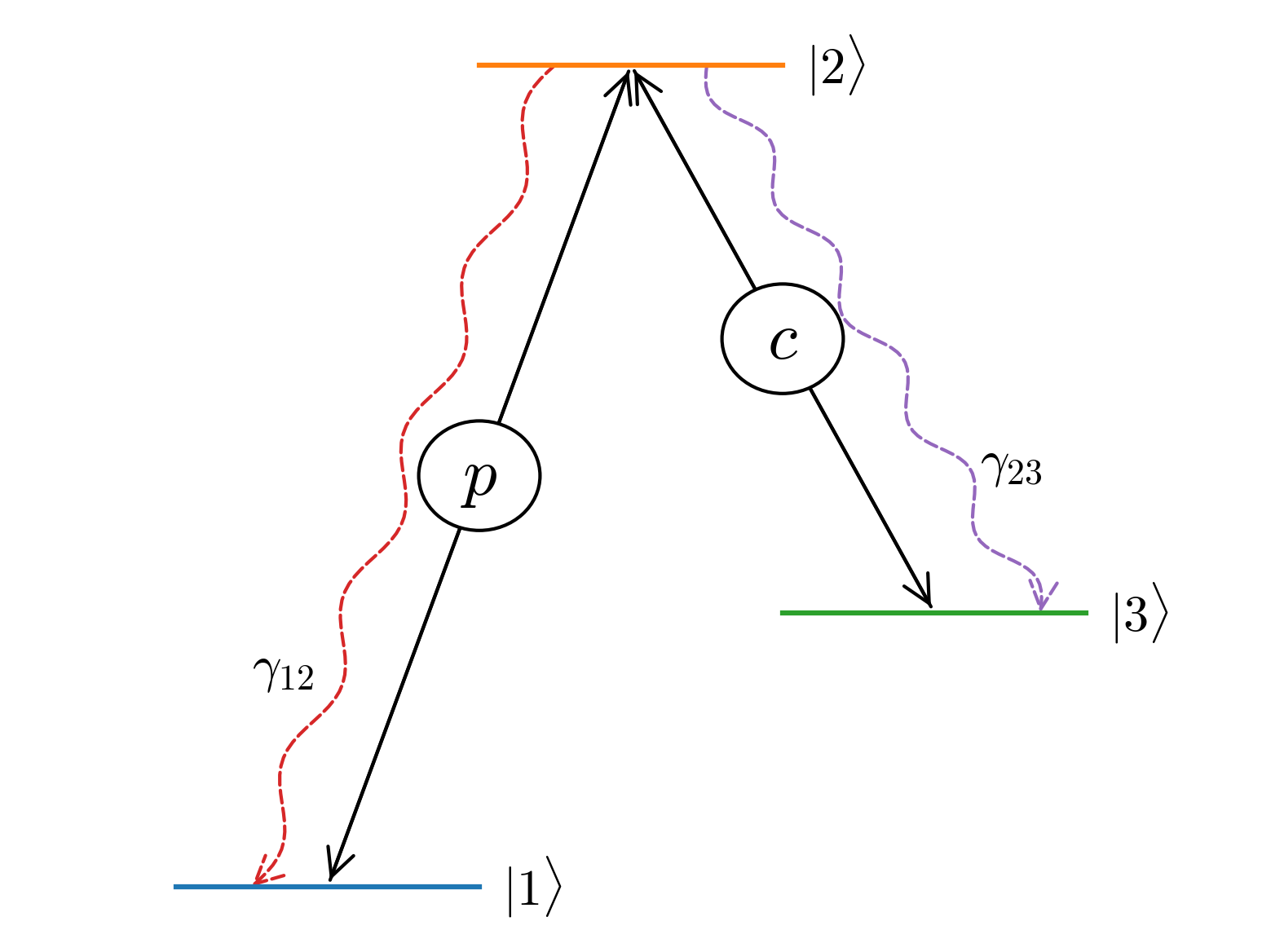
where we define as the state with the highest energy. Thus, the assumption of a -system implies that (see Figure 1). State is then coupled to states and by the following matter-radiation Hamiltonian
| (2) | |||||
which represents interactions with two monochromatic probe and control radiation fields within the dipole approximation. Thus, and are frequencies of probe and control fields, and and are their respective Rabi frequencies. Then, the time evolution operator for the time dependent system Hamiltonian is obtained by solving the following time dependent Schrödinger equation:
| (3) |
where , the identity operator in the system Hilbert space. Within RWA, is approximated as
| (4) | |||||
We denote the time evolution operator corresponding to as . The physical justification for the above RWA is that the net contribution of counter rotating term is insignificant due to cancellation of fast oscillating terms. While RWA has been used widely and makes it possible to obtain closed form expression for eigenvalues of the Hamiltonian in RWF for simple cases, as illustrated in Appendix A for the present model, actual numerical tests of RWA have been scanty. Tests of RWA provided in this work have significant implications in this respect.
In the presence of dissipation, the dynamics is no longer unitary and it is in general necessary to consider the time evolution at the level of a density operator. Under the assumption that all the dissipations are caused by weak and Markovian baths, the effects can be accounted for by a Lindblad type equation. In a recent work,[11] such a Lindblad equation was used for the study of EIT. The corresponding time evolution equation for the system density operator in the present notation can be expressed as:
| (5) |
where is the system Liouville superoperator defined as and is a Lindbladian defined as
| (6) |
In the above expression, the subscript represents the anticommutator. Thus, for any and , .
III Propagators based on Magnus expansion for periodic driving
Given that the Hamiltonian is periodic in time with period , for and any positive value of integer . As a result, in practice, explicit calculation of for only suffices. This is because for any value of , the following relation holds:
| (7) |
where .
For the calculation of for , we employ an expression based on the ME for the differential operator, , where , for a small enough value of . See Ref. 19 and references therein for details of how these expressions can be derived. Thus, we first determine for at each discretized by repeated multiplication of . Once is determined this way, it is possible to make large (stroboscopic) jumps corresponding to the size of the period. This results in orders of magnitude of savings in terms of calculating matrix exponentials and commutators, and makes the calculation of long-time dynamics feasible. The dynamics at intraperiod points (micromotion) can then be determined using Eq. (7). If the major focus is the steady state limit, even further acceleration is possible by using the approach of numerical matrix multiplication,[21] namely, using the fact that for any positive integer .
Conceptually, our approach is similar to the Floquet-ME.[22, 23, 24] In fact, the time evolution operator for a single period, , corresponds to the unitary operator for the Floquet Hamiltonian[23] (sometimes referred to as the average or effective Hamiltonian[25]) defined as follows:
| (8) |
For practical purposes, our numerical procedure for solving the Floquet problem has some advantages compared to the approach to determine . For instance, it has been noted that the Floquet-ME may require high order approximation for reasonable accuracy,[24] which may only be possible for simple Hamiltonians. In addition, truncation of the Floquet-ME beyond the first order produces a dependence of the eigenvalues of on the initial point (referred to as the Floquet gauge), which makes them no longer related by a unitary transformation.[23] Finally, our procedure enables calculation of the intraperiod motion as well, from which detailed time dependences in the long time limit can be identified (see Fig. 6). The procedure above allows for calculation of the density-operator for the closed-system dynamics by using . For the open system case, we can use the time evolution operator of the density operator in the Liouville space to achieve similar exponential speedup, as detailed in the next section.
IV Magnus Expansion in the Liouville space for open system
Here, we provide description of how the system density operator can be propagated in the Liouville space, for both cases of closed and open systems. For the closed system, the dynamics is governed by only (no term) in Eq. (5). The explicit definition of this system Liouvillian in the Liouville space can be found from the corresponding definition in the Hilbert space by using the superket triple product identity,[26] as defined in Appendix C. Thus, in the Liouville space is defined as
| (9) |
where is the identity operator in the system Hilbert space. Thus, the density operator vector in the Liouville space at time is given by
| (10) |
where the second equality defines the time-evolution superoperator in terms of given by Eq. (9).
For the open-system dynamics, the full equation, Eq. (5) is used. The corresponding expression for the Lindbladian in the Liouville space is
| (11) | |||||
where for each represents a jump operator (in the system Hilbert space), and are respectively defined as , = , = , and = . The expression for each coefficient in the above equation can be found from Eq. (6). For this open system dynamics, the time-evolution of the system density operator vector in the Liouville space is given by
| (12) | |||||
where the second equality serves as the definition of .
To numerically solve for or , we applied the 6th order ME-based expression we have derived recently.[19] For the former (closed system dynamics), this is equivalent to calculating with the 6th order expression for . For the latter, more details are provided in Appendix C. In complete analogy with the time evolution-operator in the Hilbert space, the calculation of and can be sped up by using Eq. 7.
(a)
(b)
(c)
(d)
(a)
(b)
(c)
(d)
(A-I) (A-II)
(B-I) (B-II)
(C-I) (C-II)
(a)
(b)
(c)
(d)
(a) (b)
(c) (d)
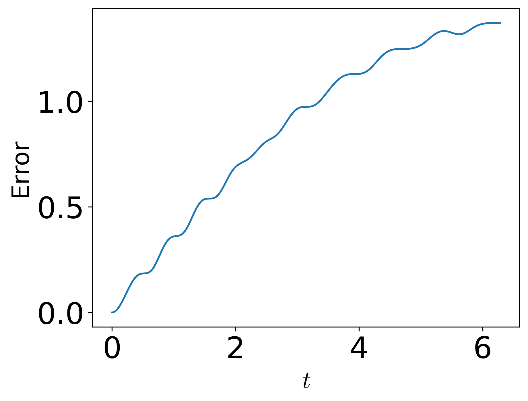
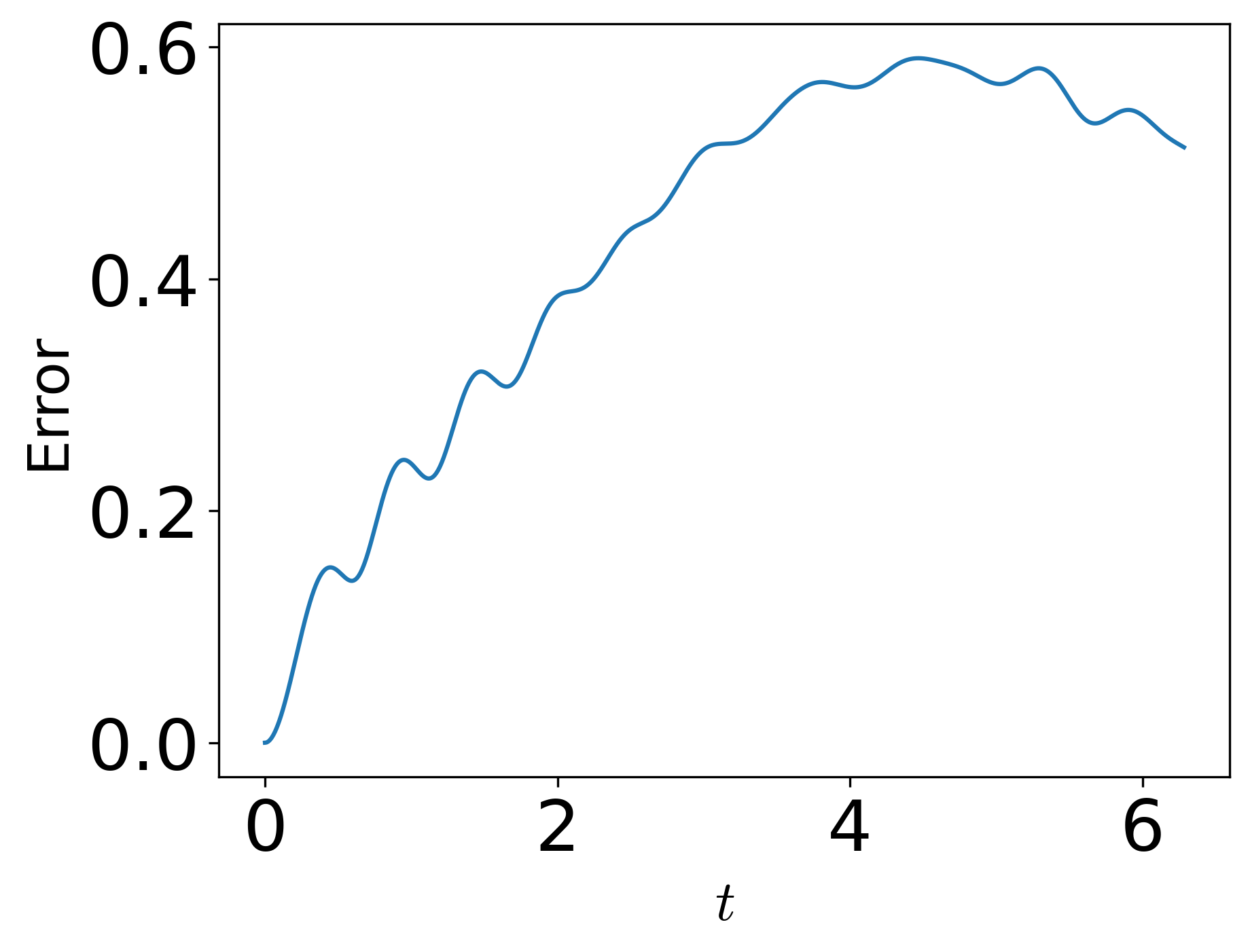
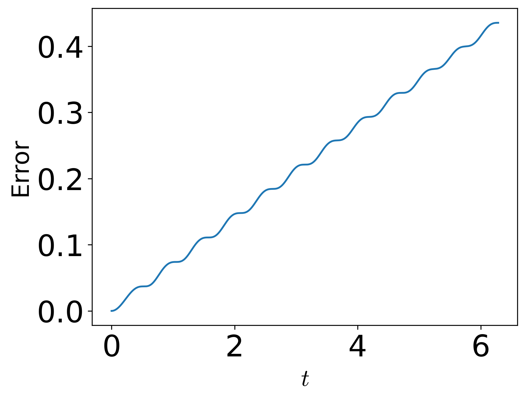
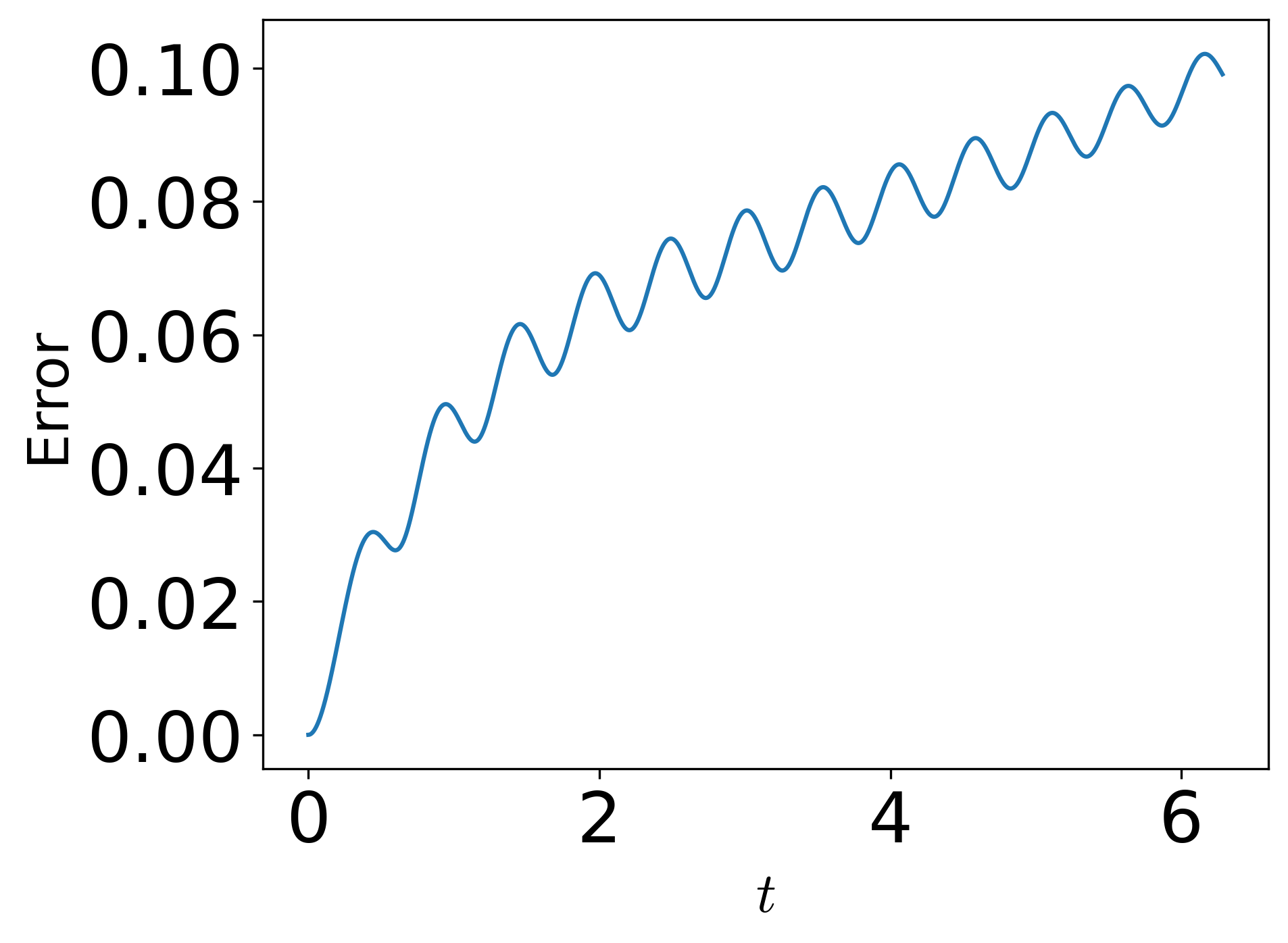
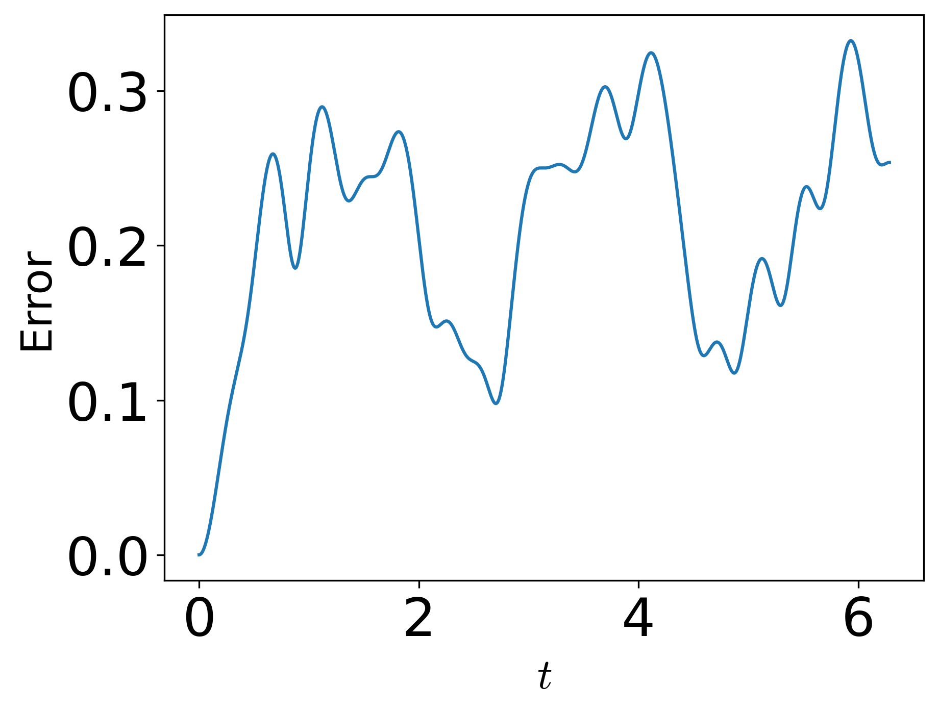
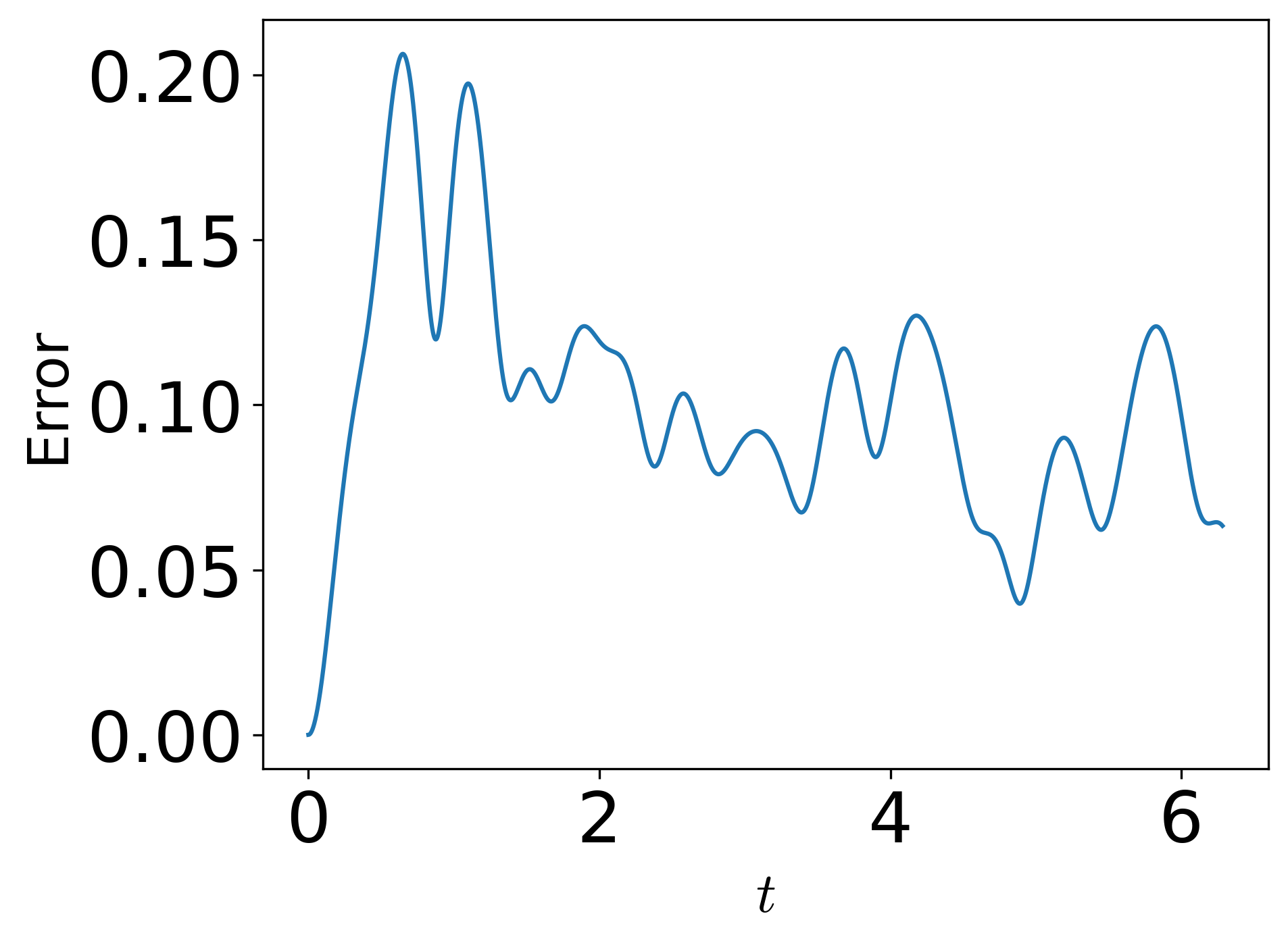
The error associated with each calculation based on RWA is quantified as follows:
| (13) |
where is the system density operator evolving for the RWA Hamiltonian defined by Eq. (4) and the subscript denotes the Frobenius measure defined, for an operator , as follows: , with and denoting the index of a matrix element of in the basis of , , and .
V Numerical Results
We conducted numerical calculations for three cases of the parameters of the Hamiltonian. Case A represents moderately strong control and probe fields whereas case B corresponds to weak control and probe fields. For case C, the control field is very strong whereas the strength of probe field is moderate. For each case, we considered both closed unitary system dynamics without bath (I) and open system nonunitary dynamics (II) with couplings to photonic bath, for which the density operator evolves according to Eq. (5). The complete set of parameters are listed in Table LABEL:table-1. The units were chosen such that . Unless stated otherwise, we assume the two-photon resonance (TPR) condition with zero detuning[27] where and . For these parameters, . For the calculation of the propagator, we used the sixth-order propagator[19] for . As the initial condition, we used .
| Case | ||||||
|---|---|---|---|---|---|---|
| A-I | ||||||
| A-II | ||||||
| B-I | ||||||
| B-II | ||||||
| C-I | ||||||
| C-II |
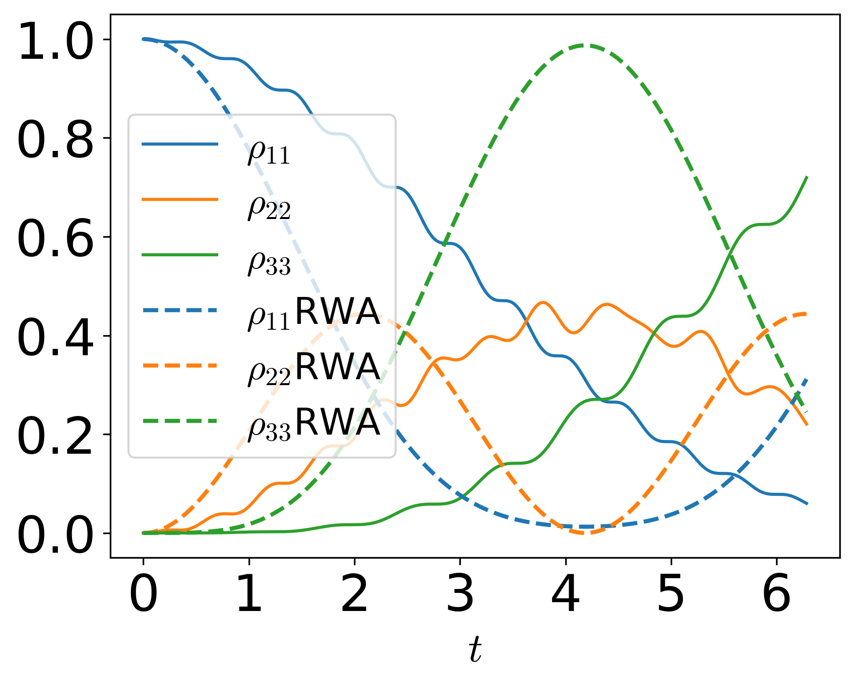
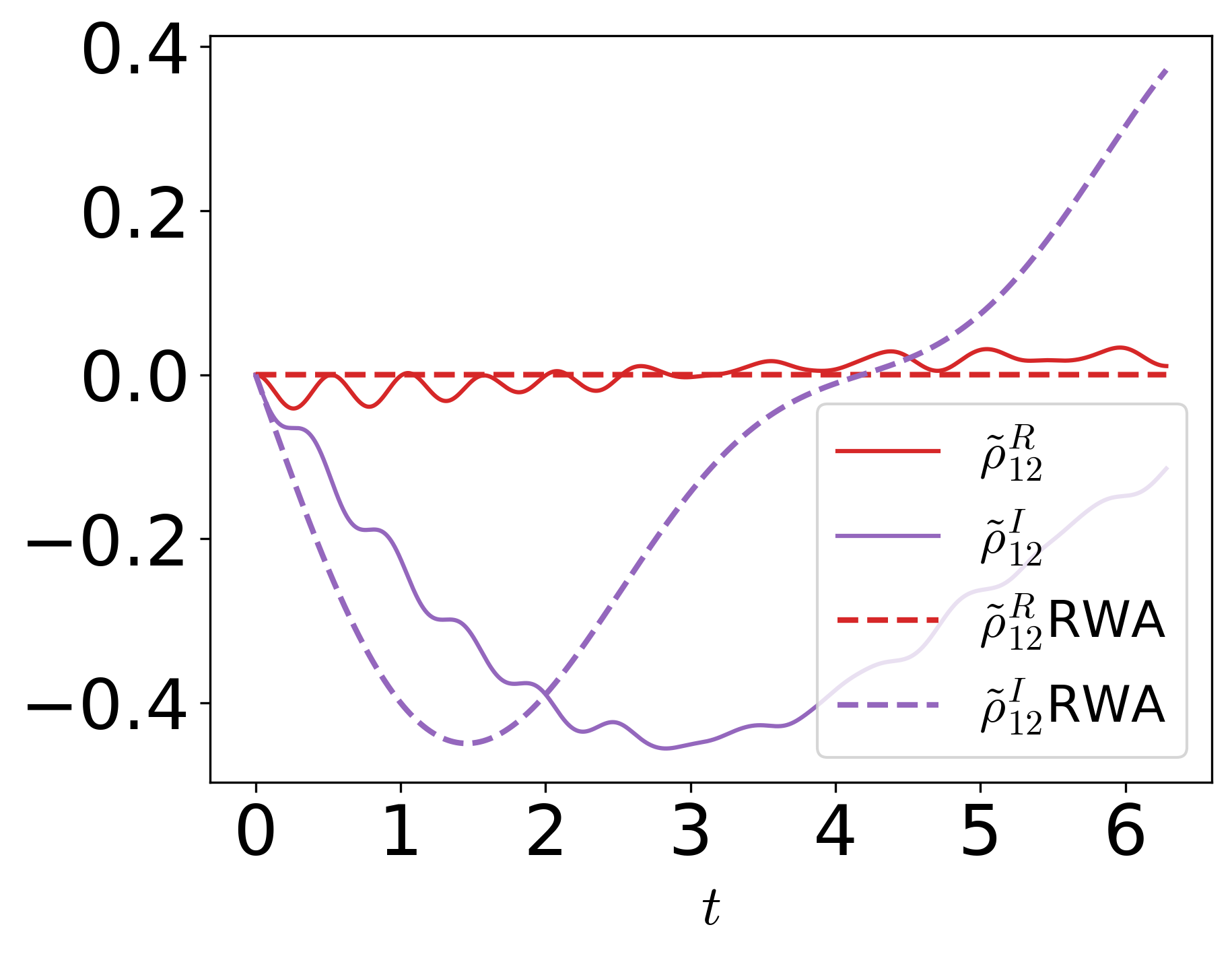
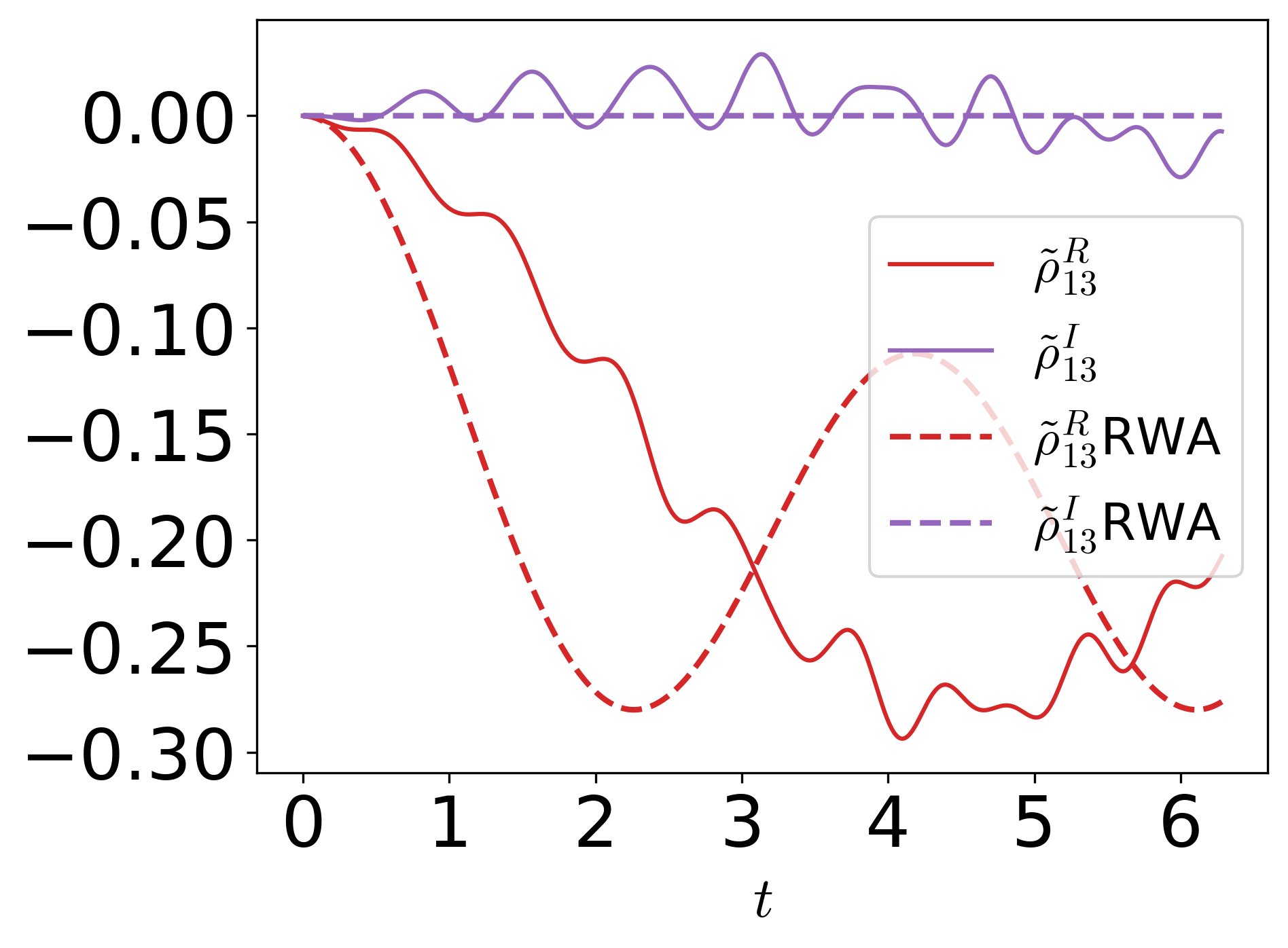
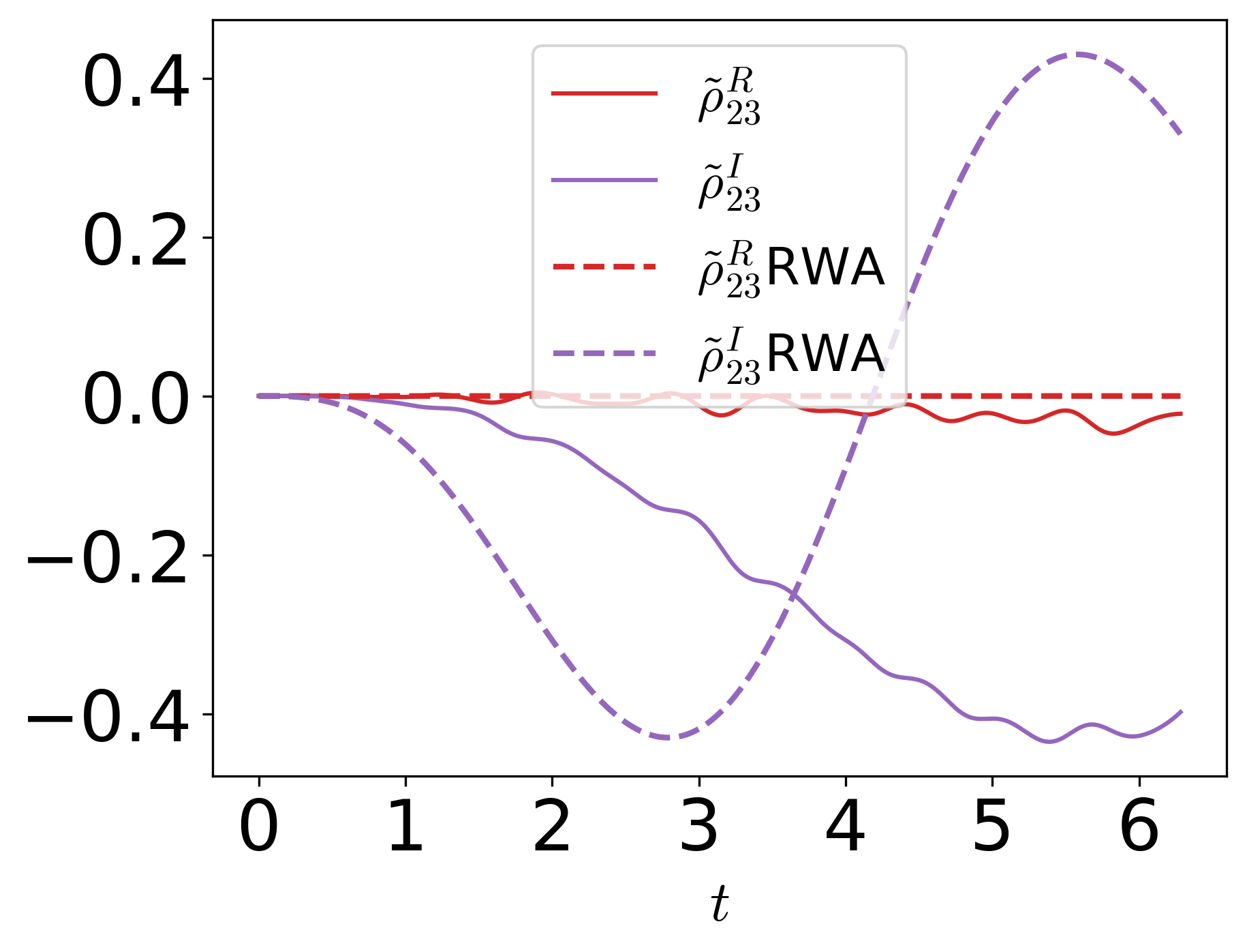
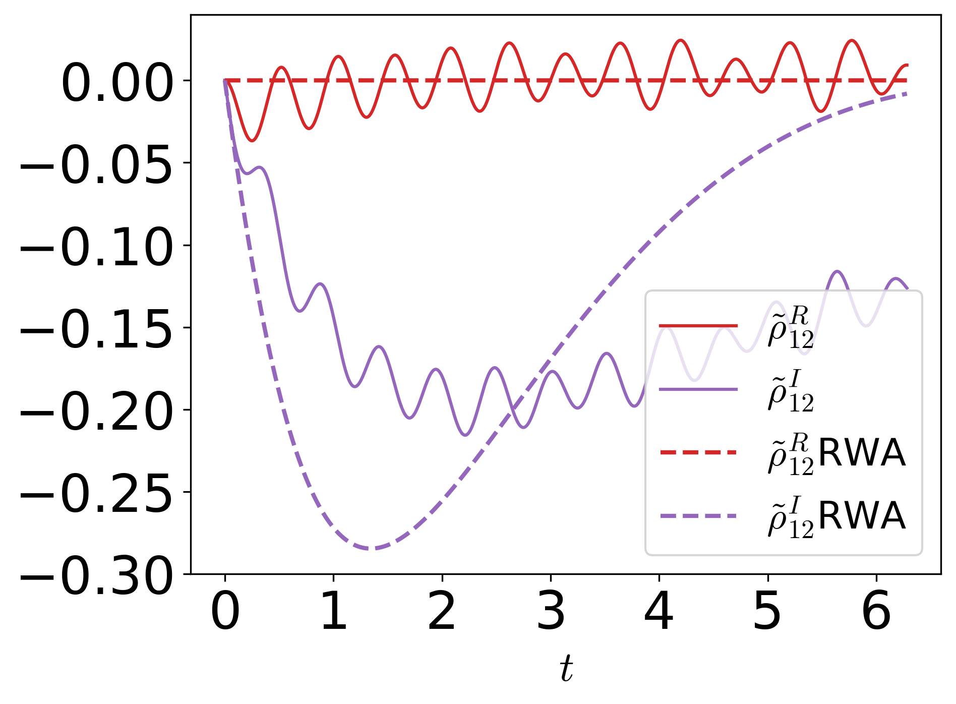
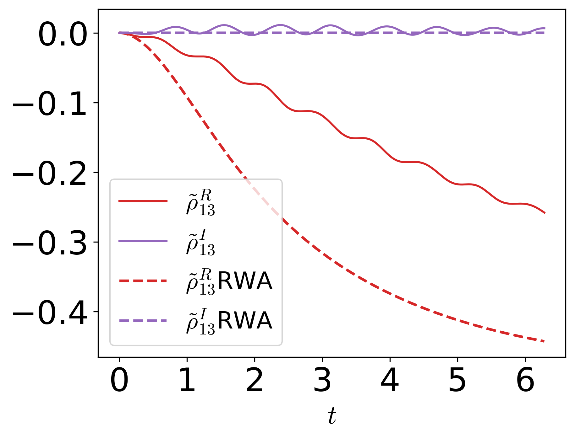
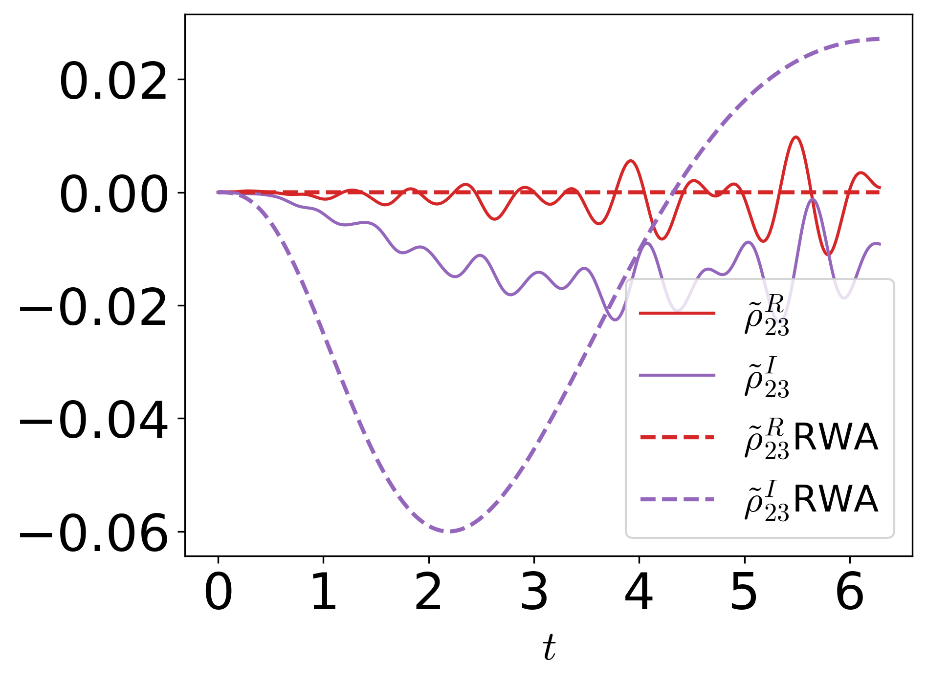
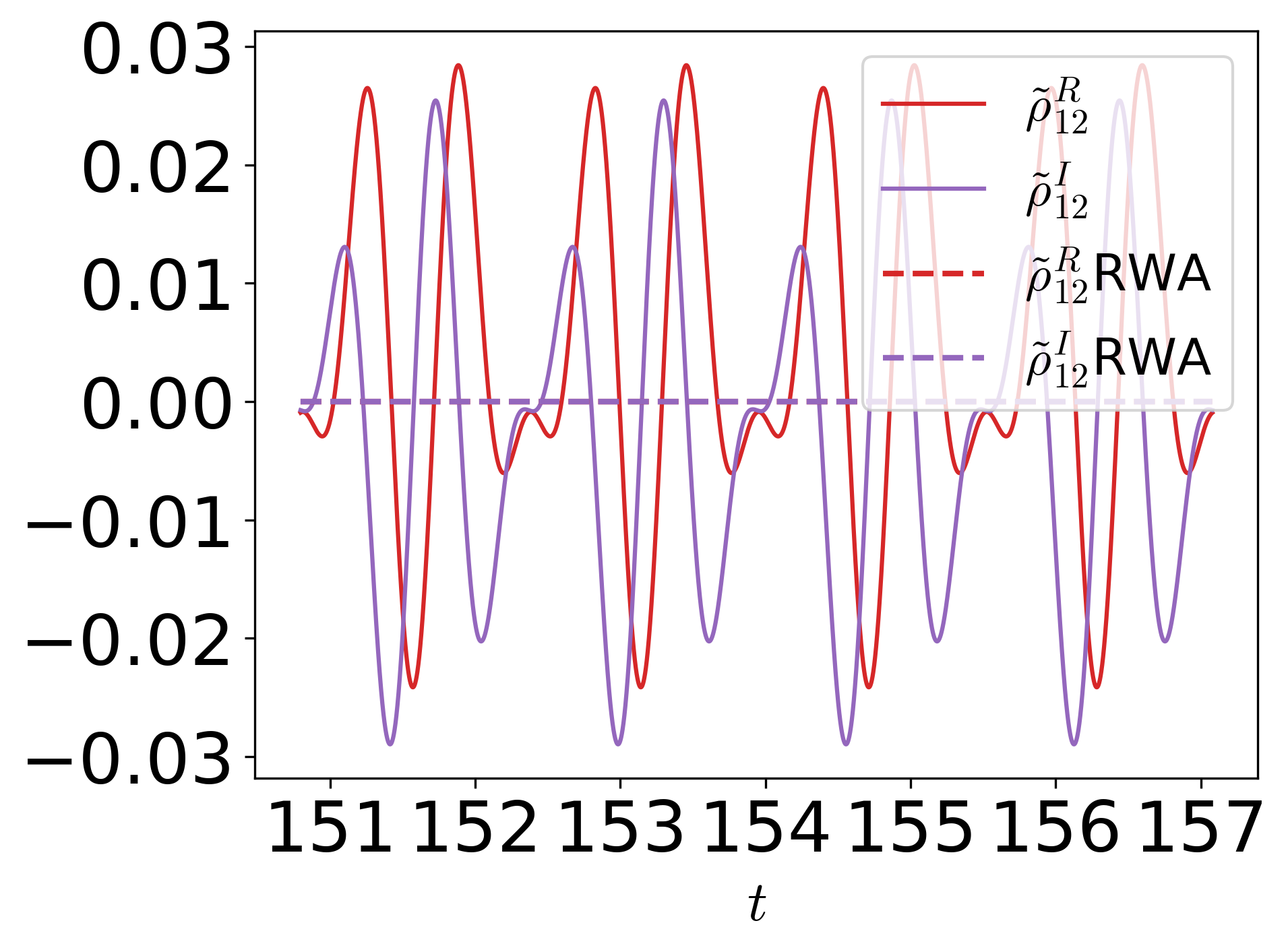
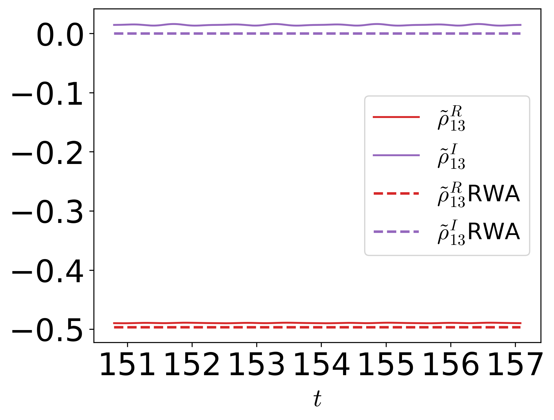
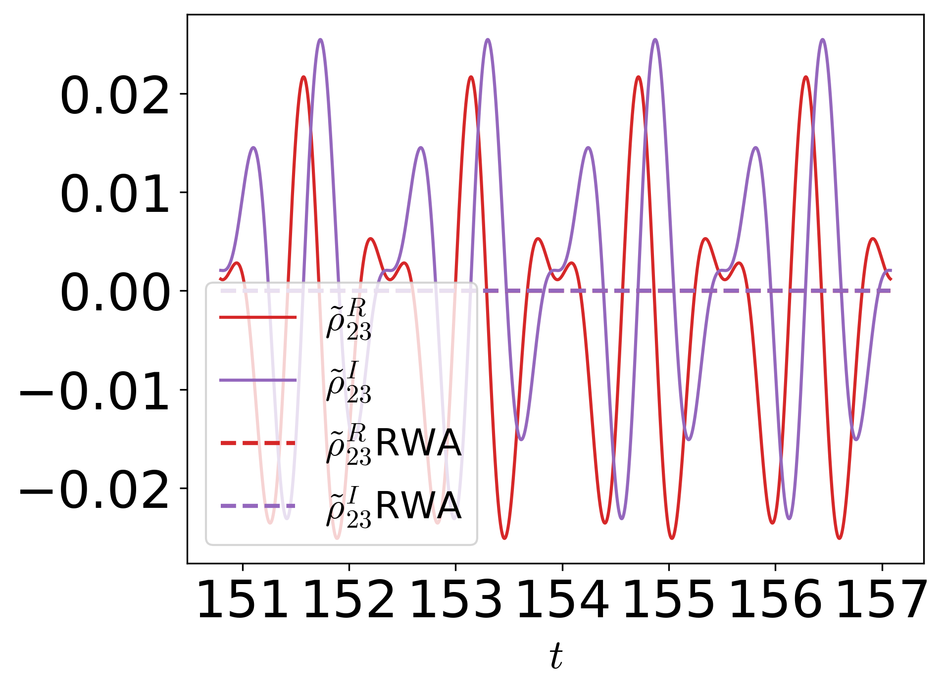
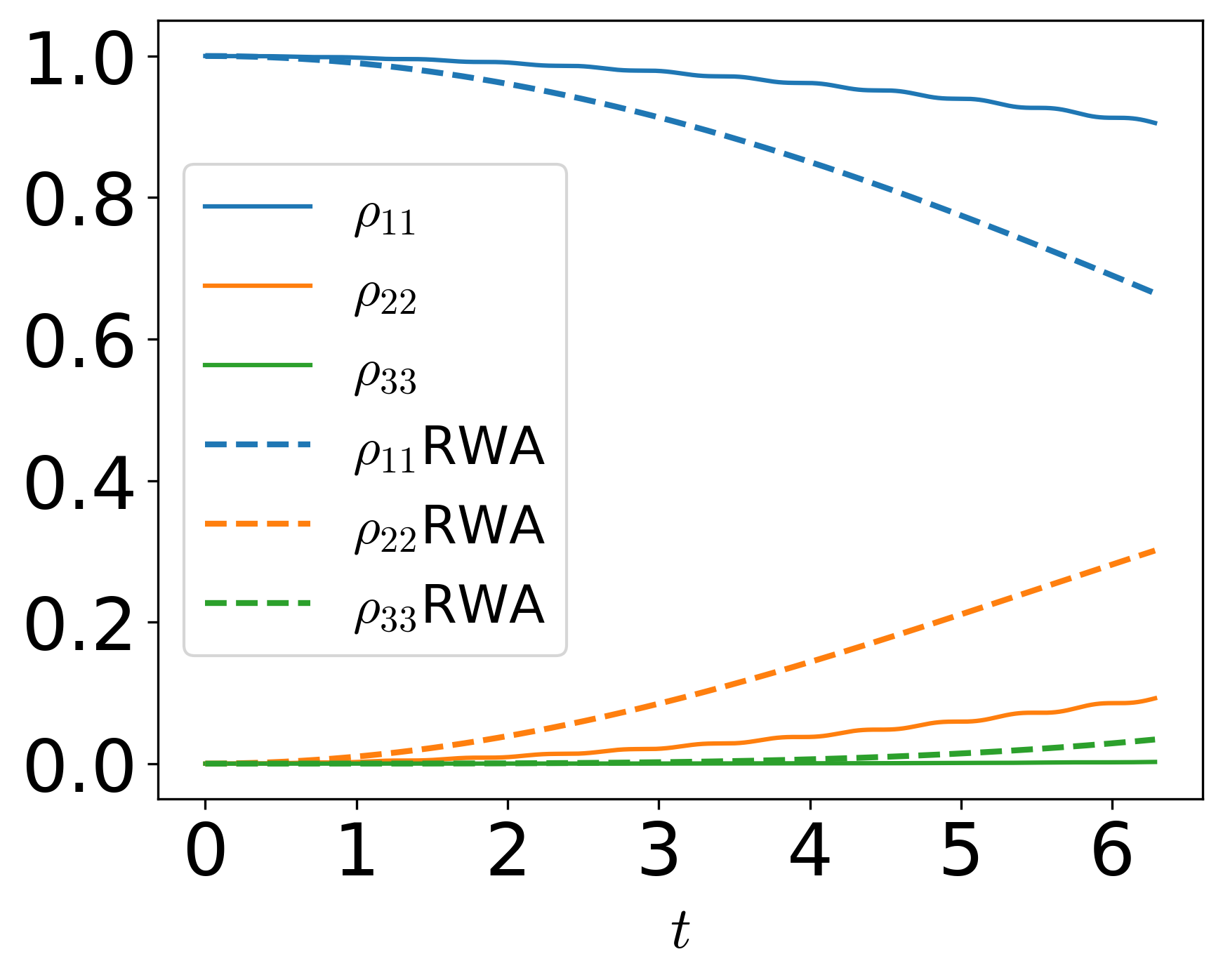
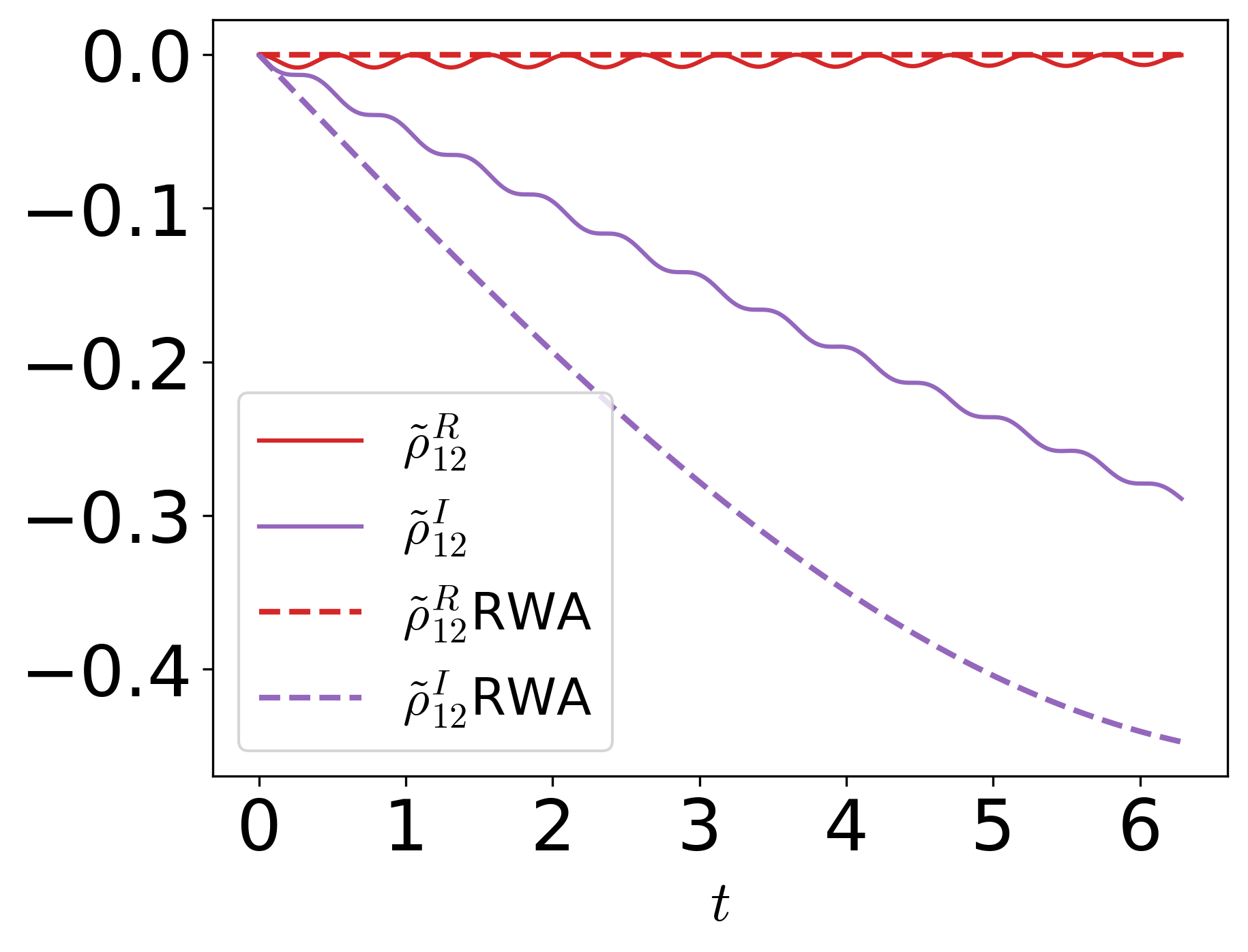
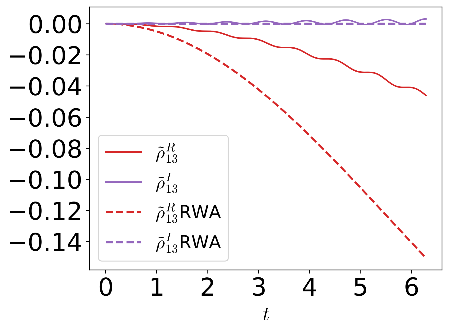
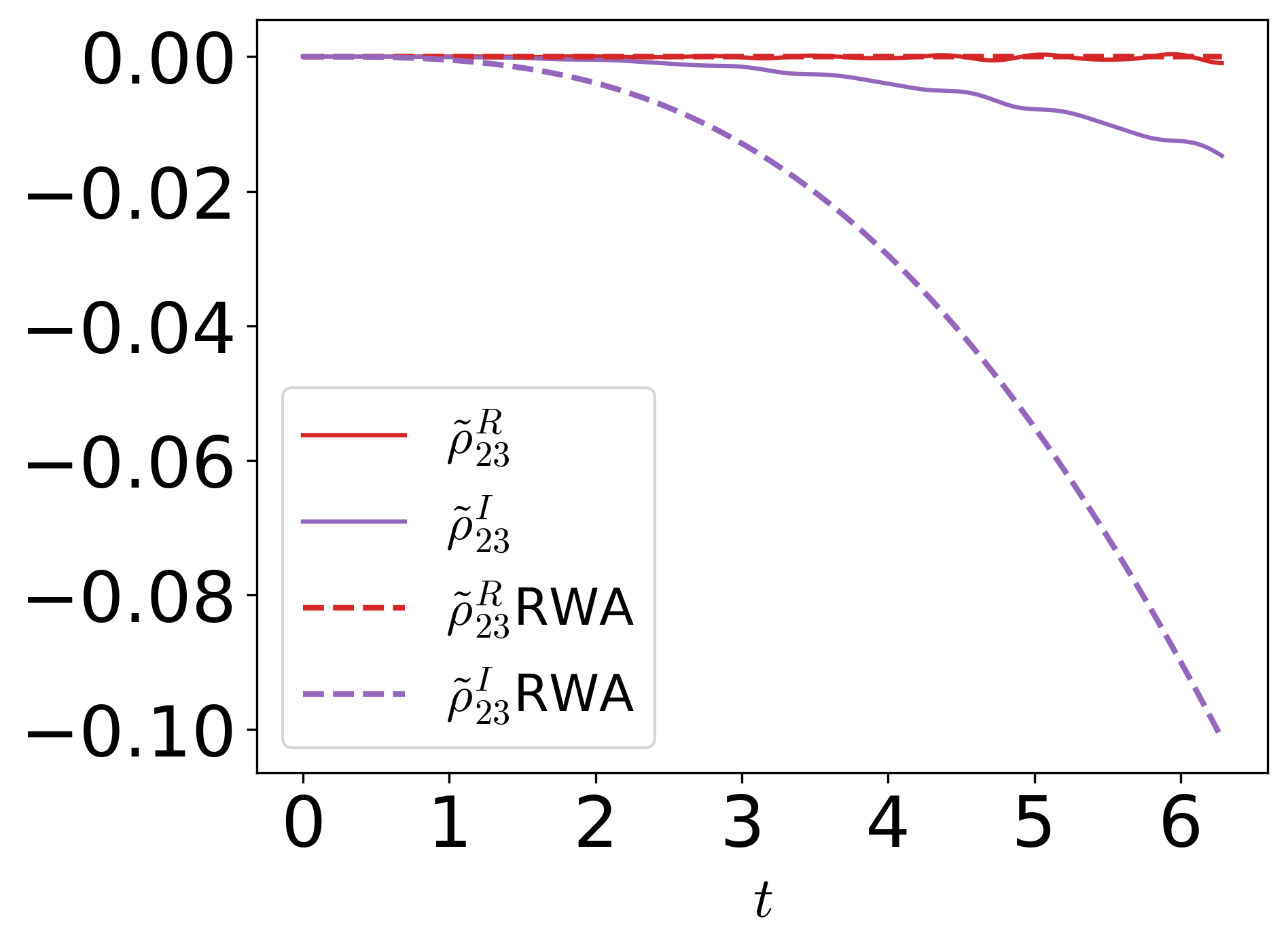
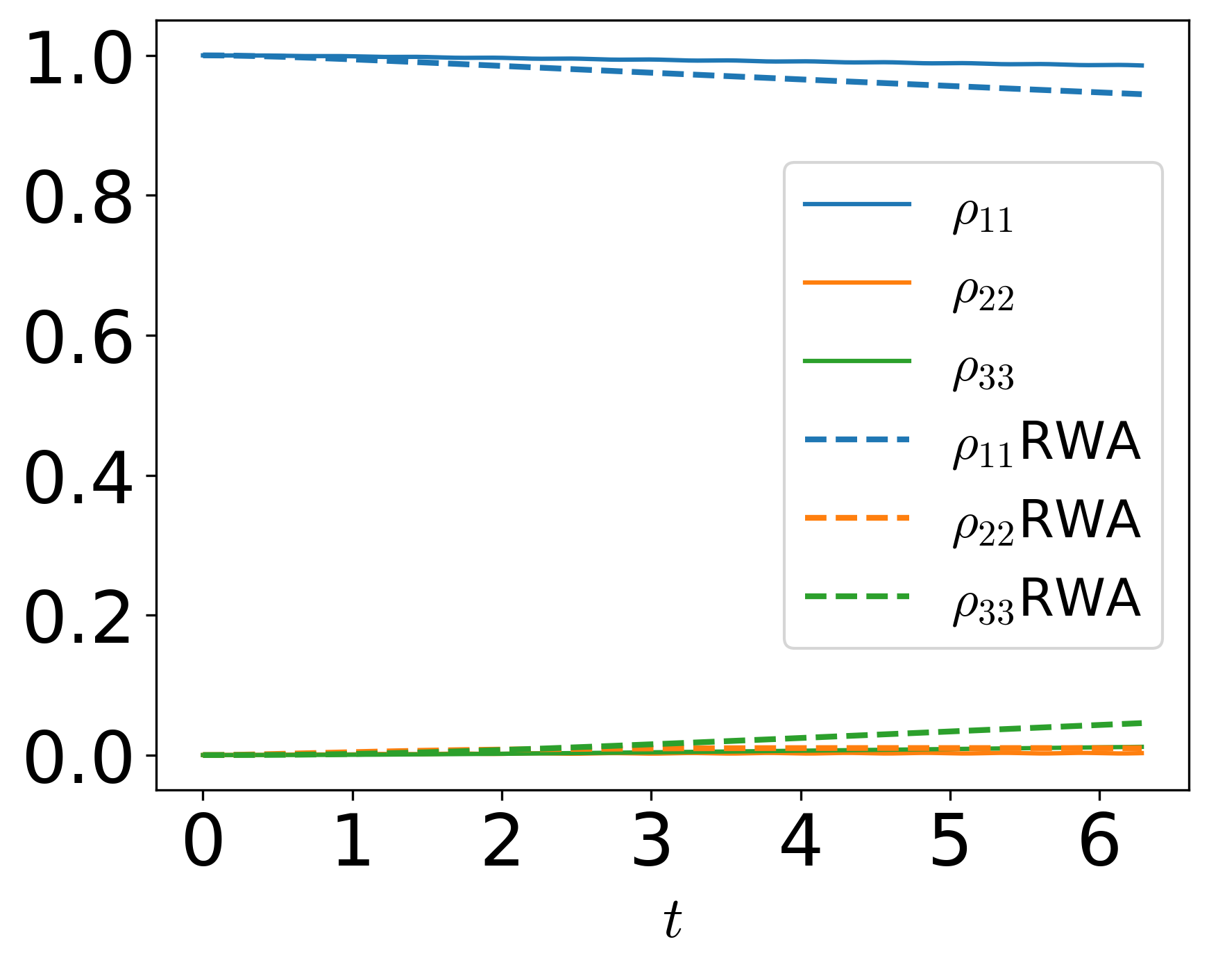
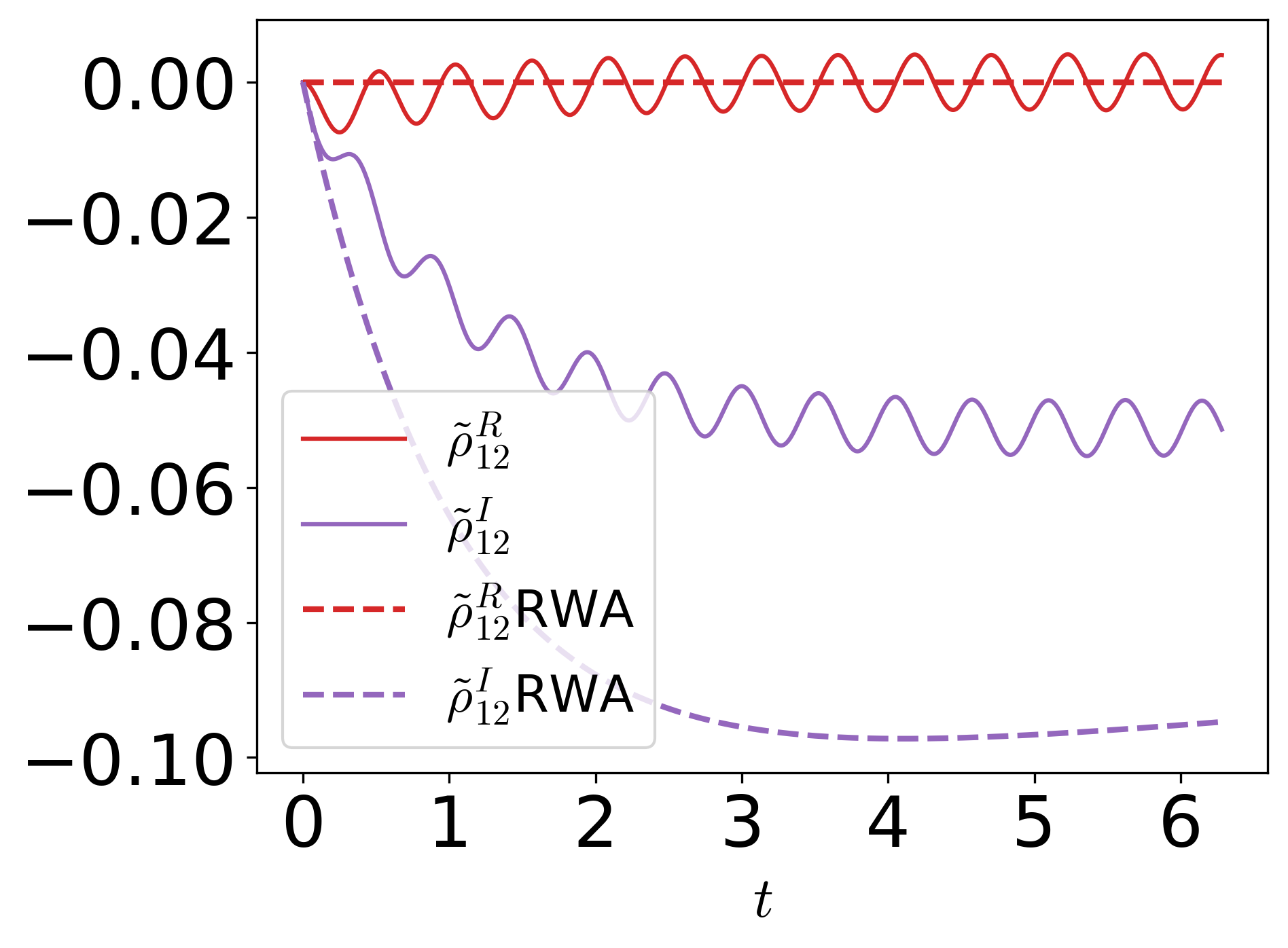
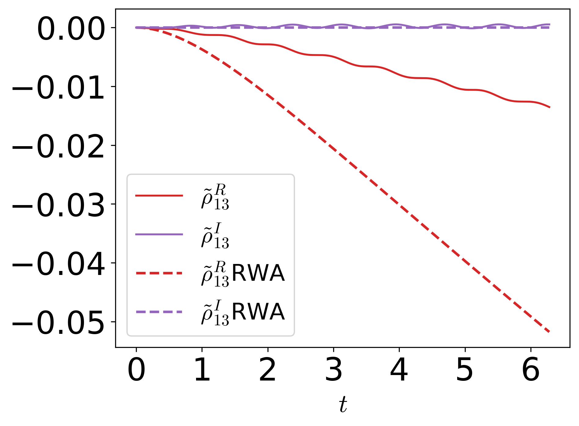
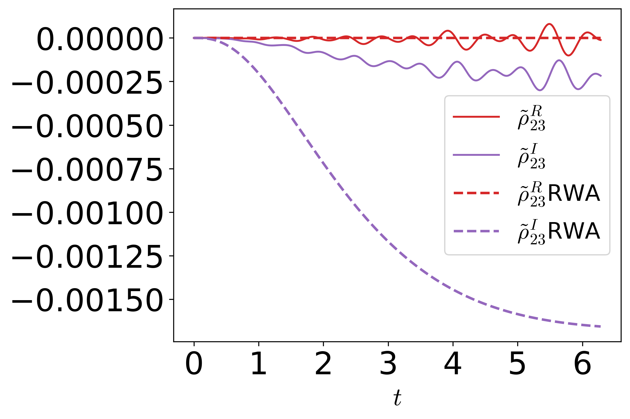
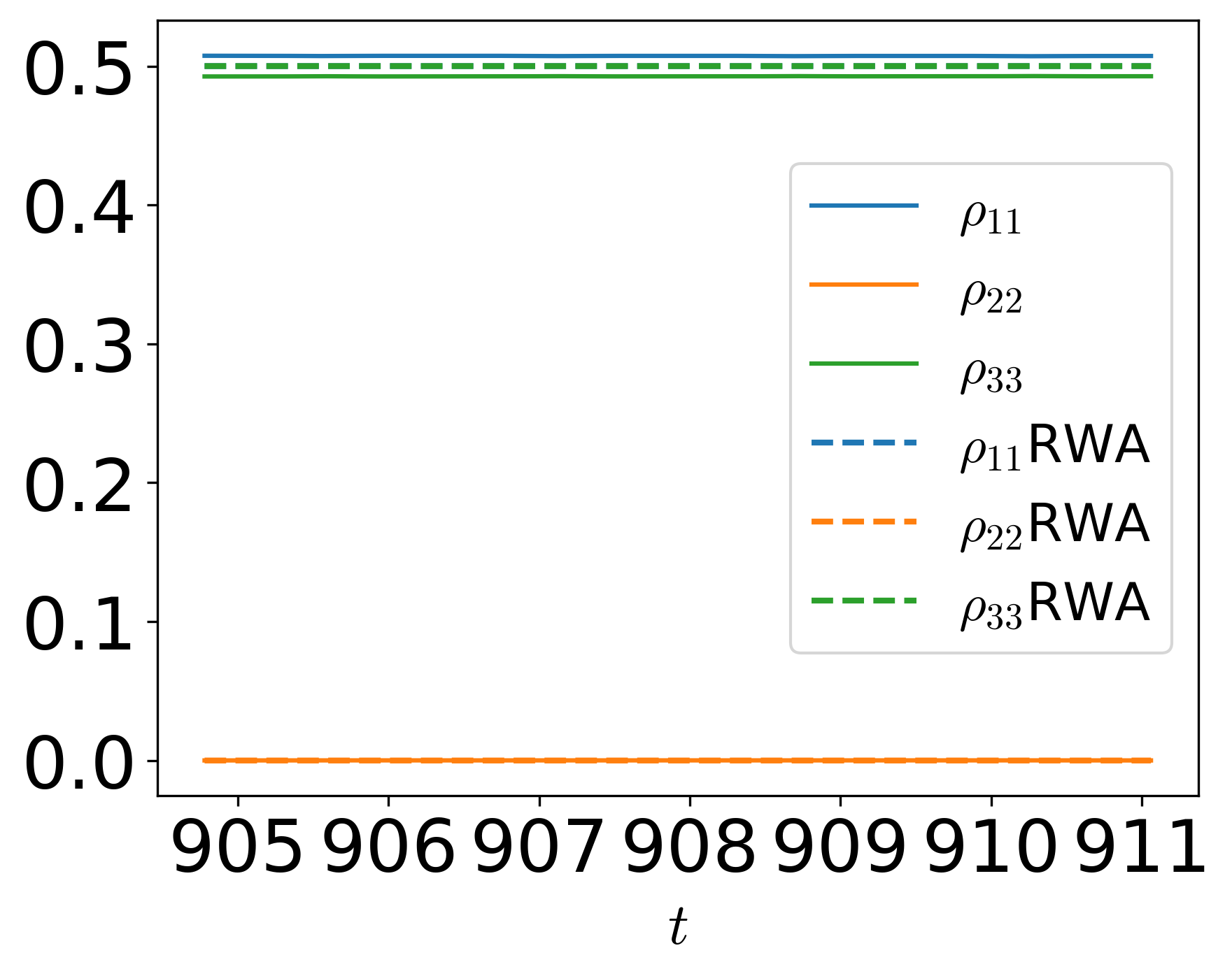
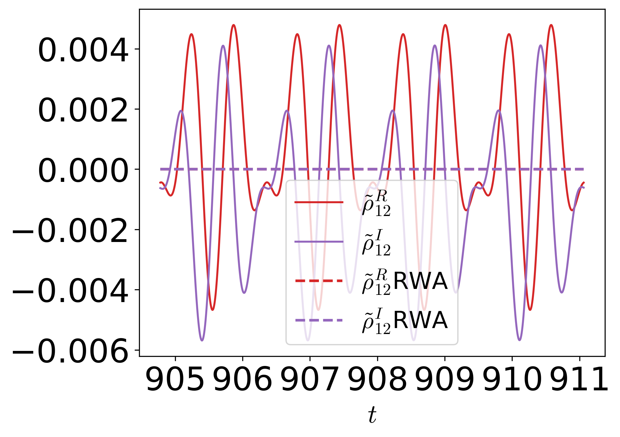
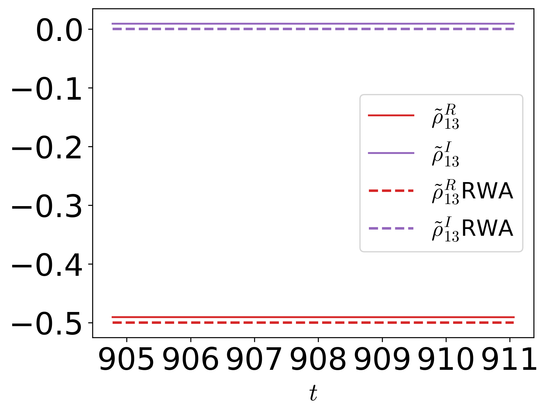
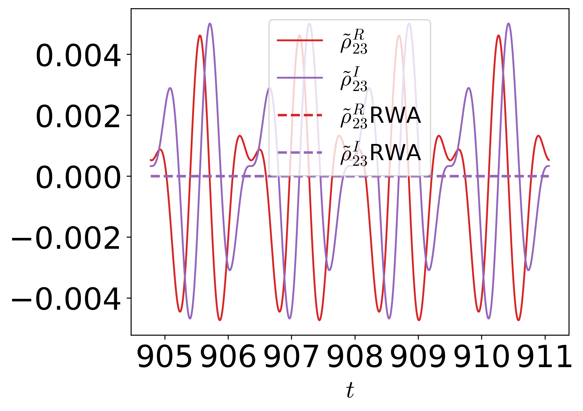
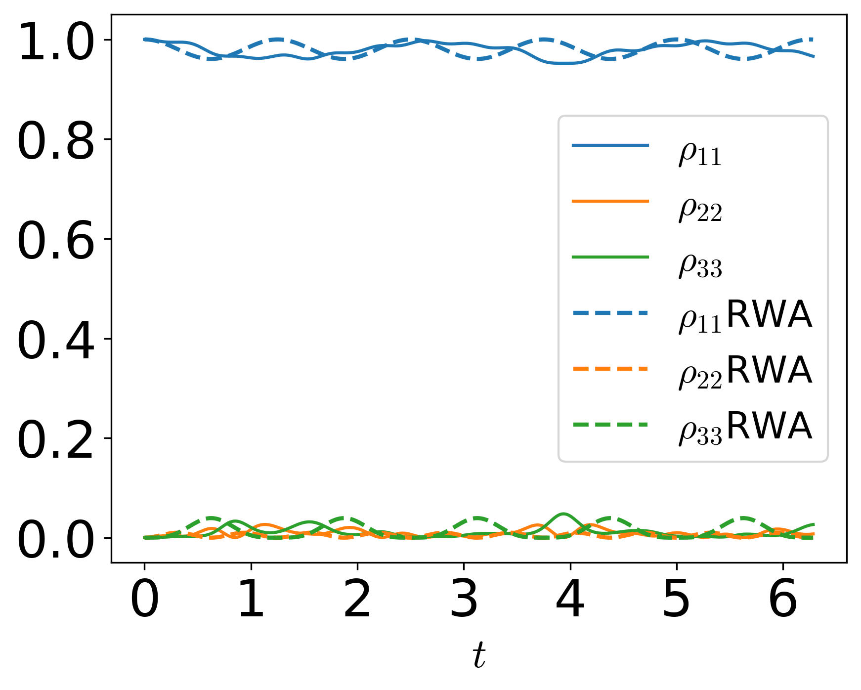
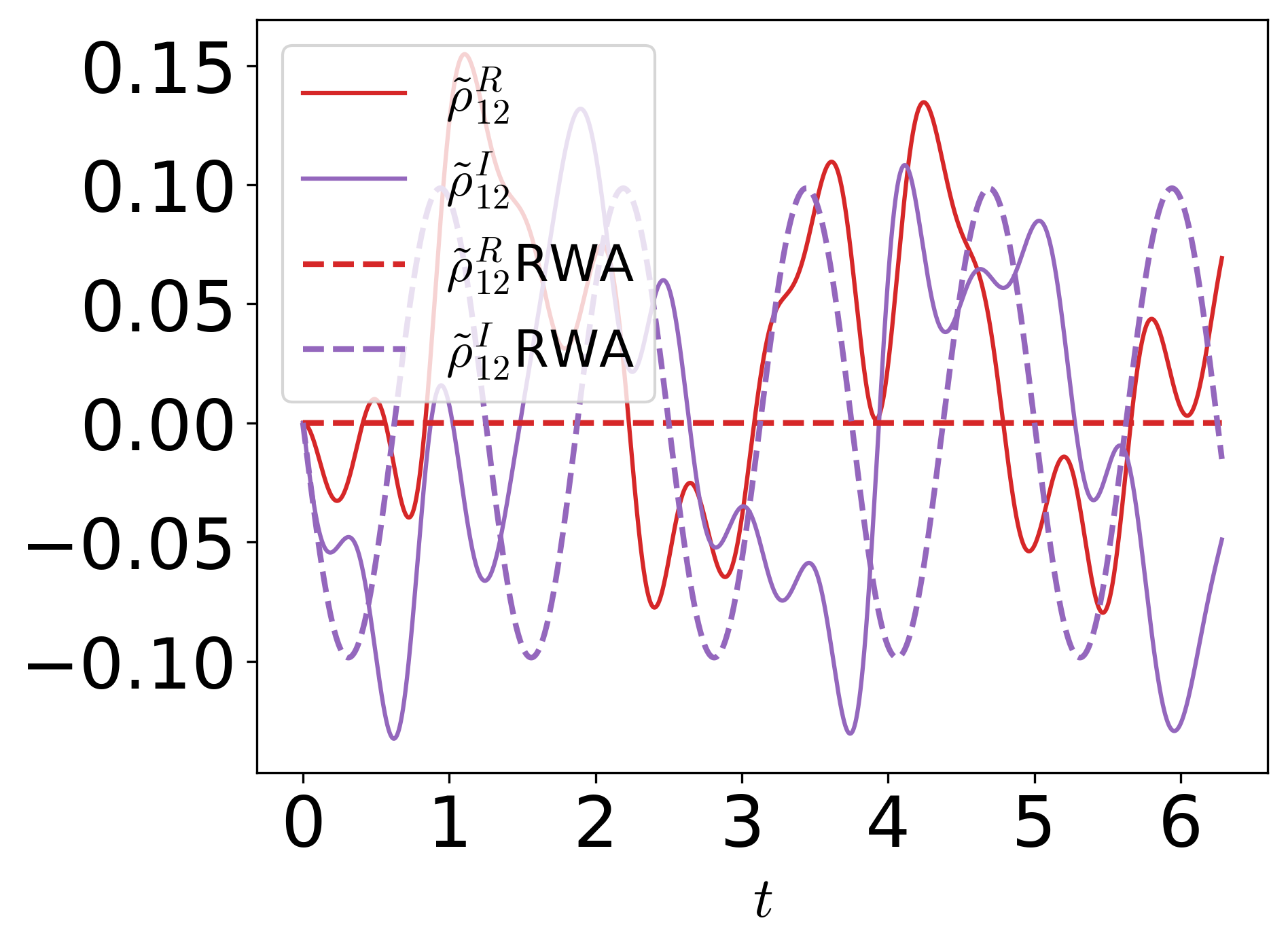
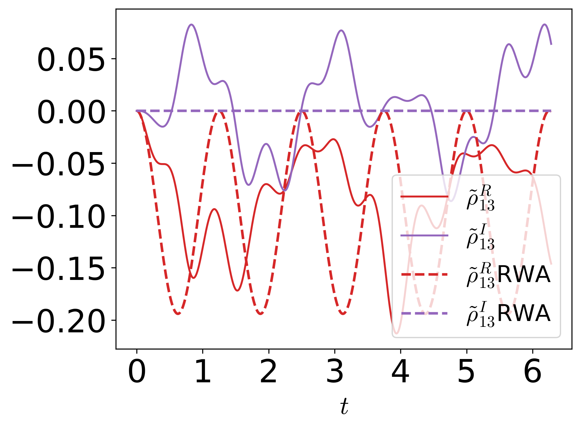
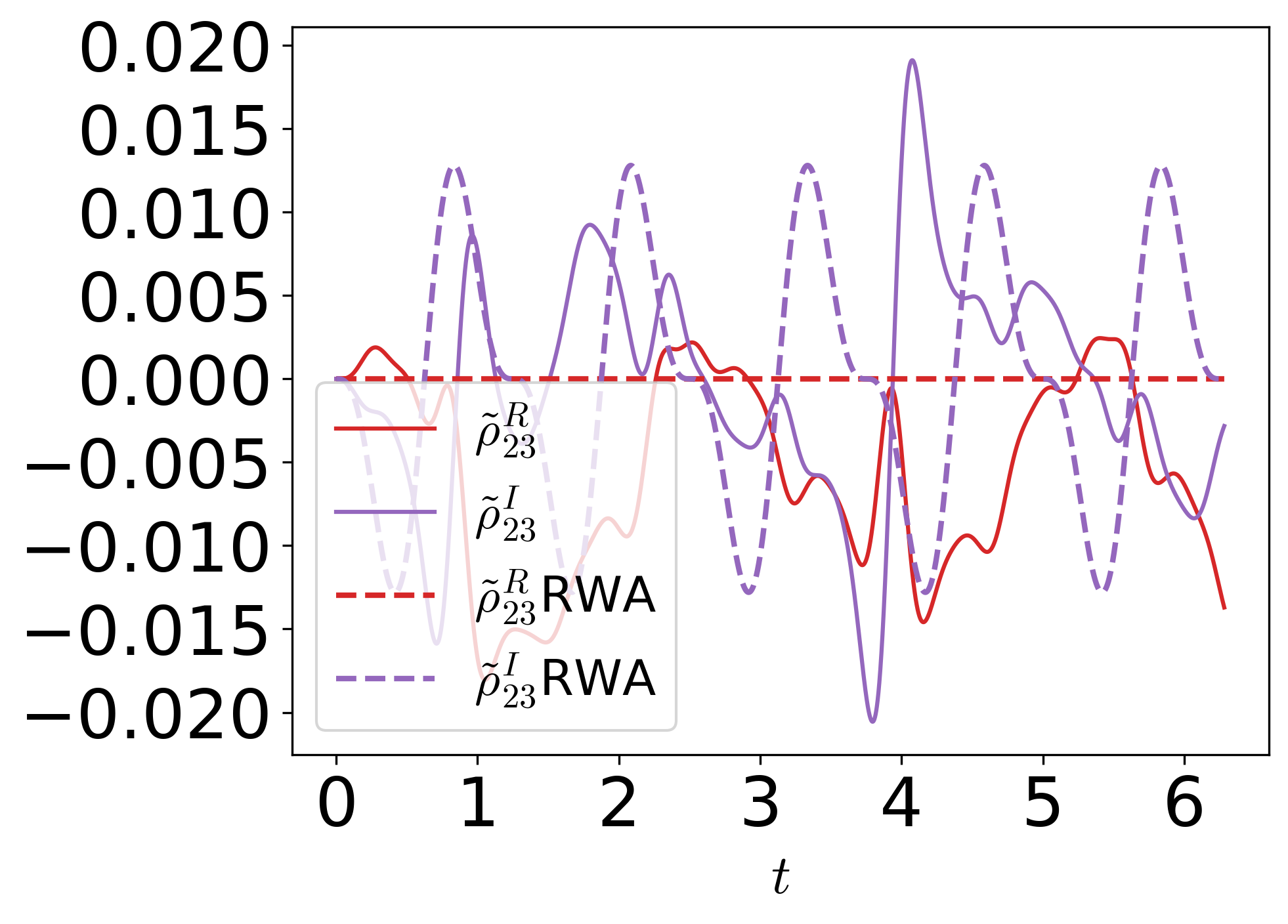
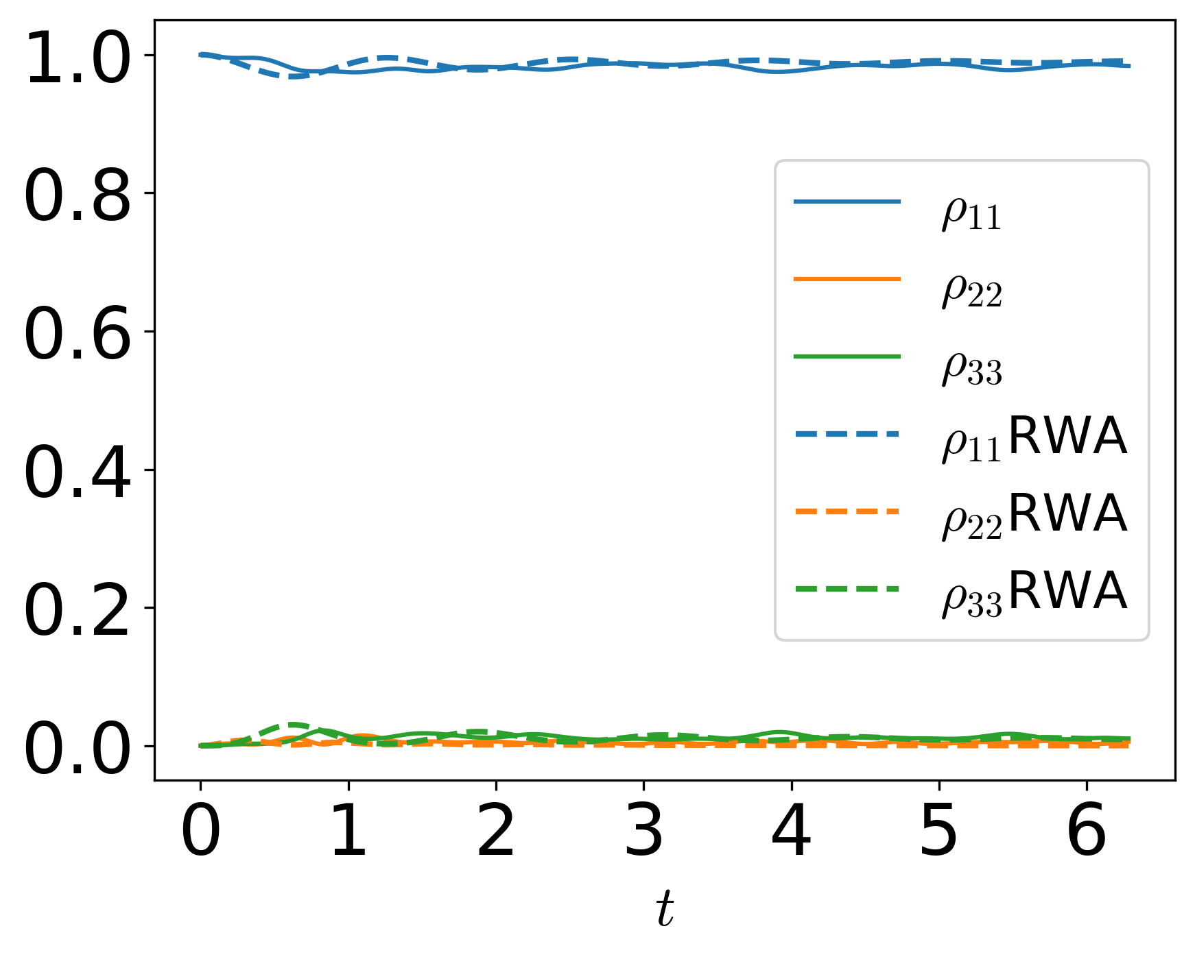
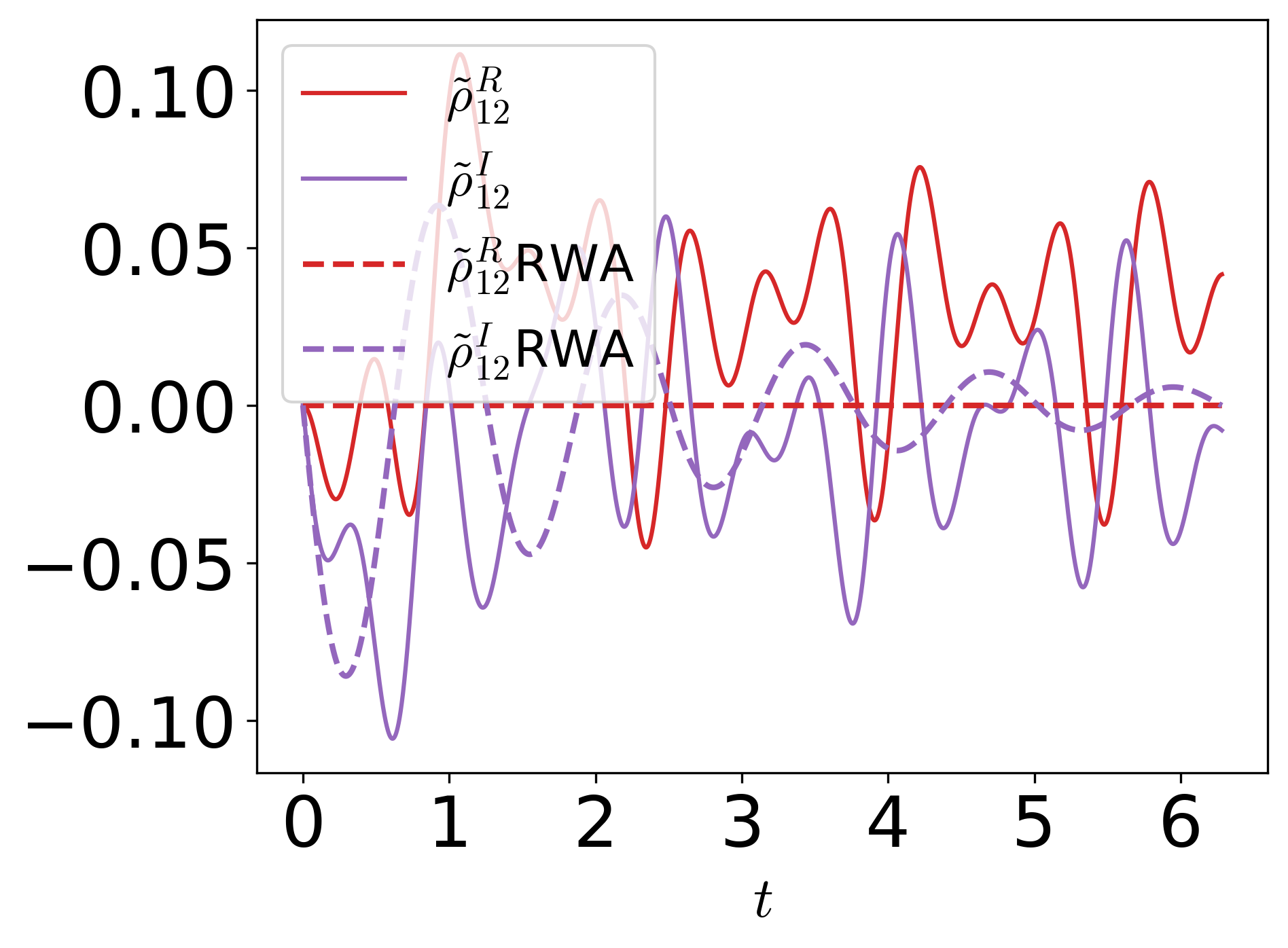
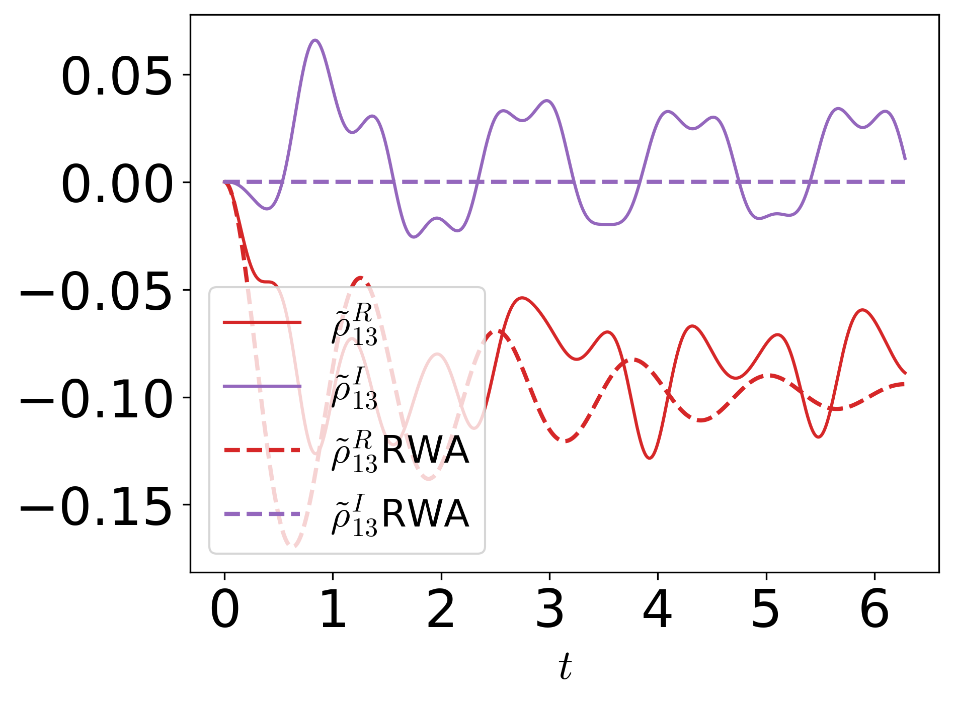
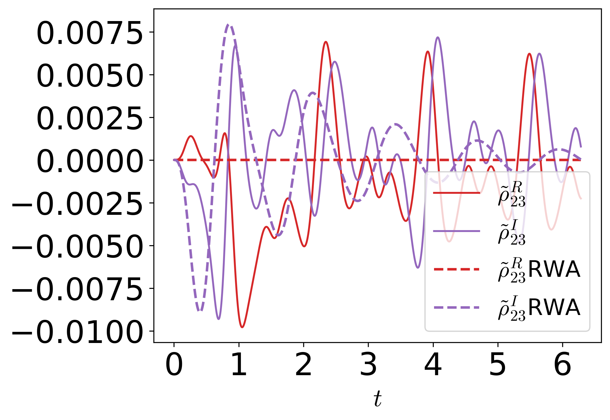
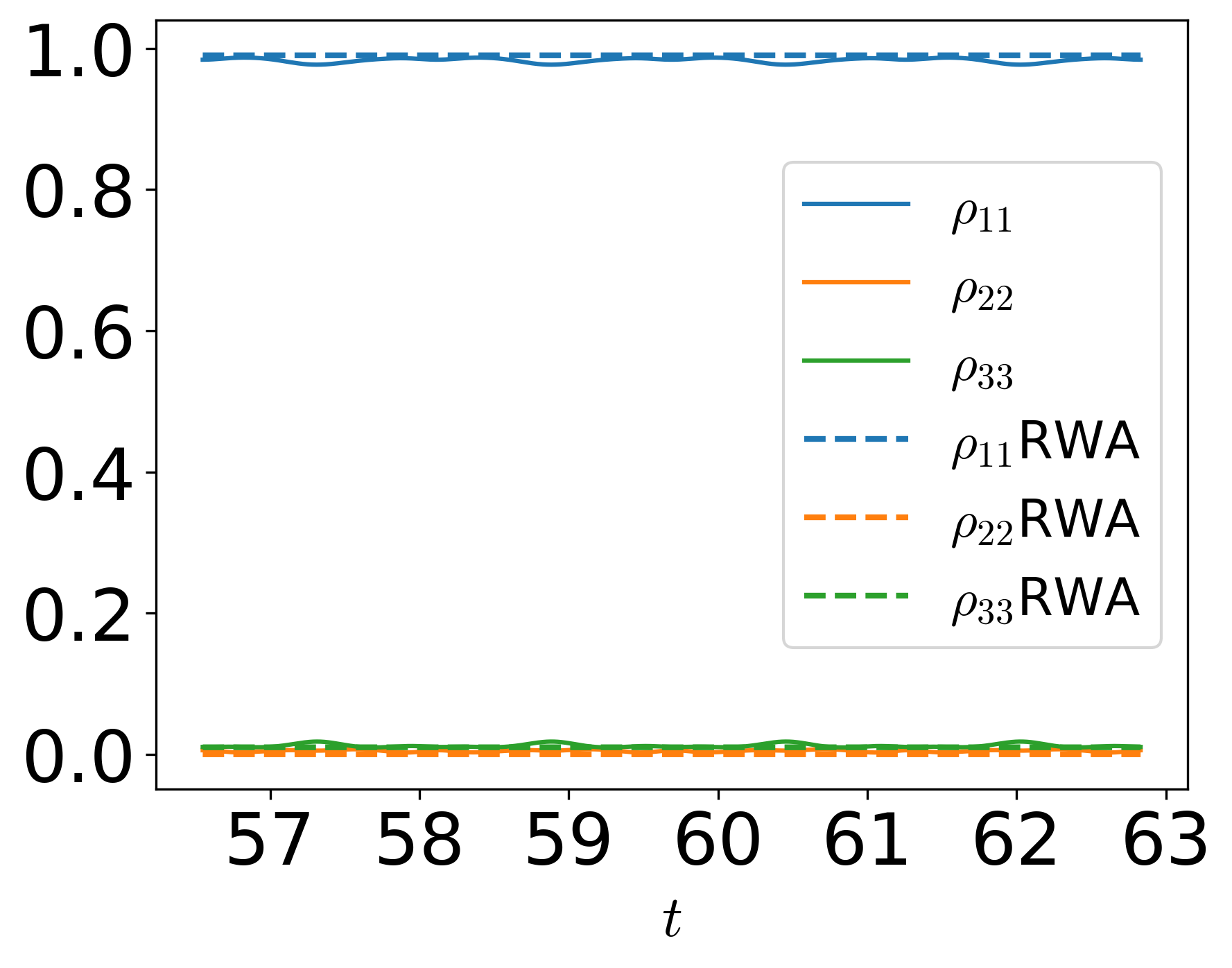
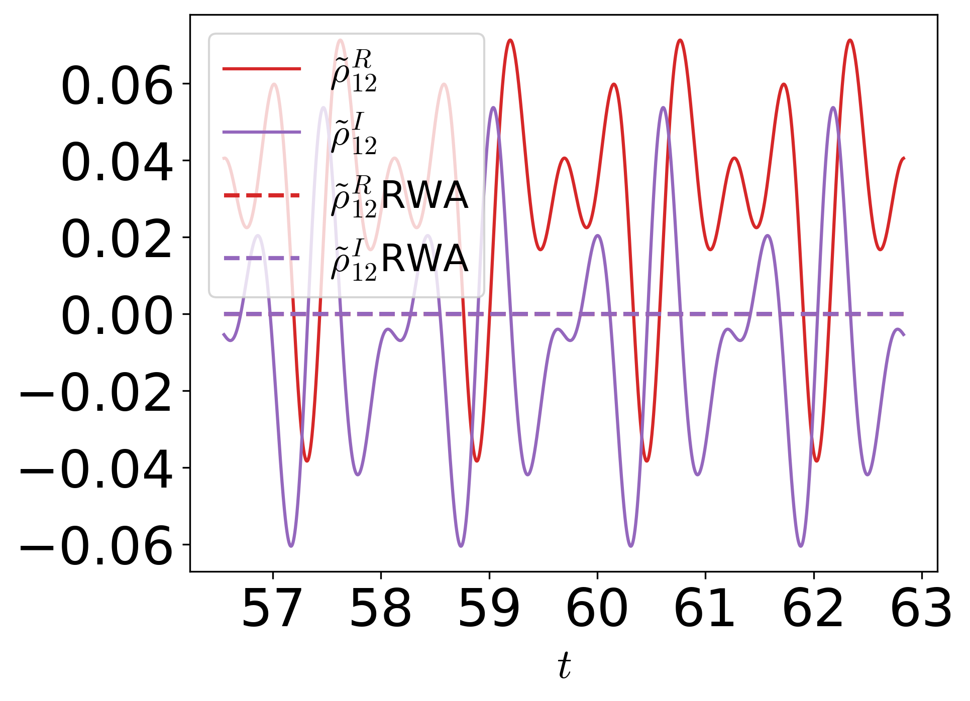
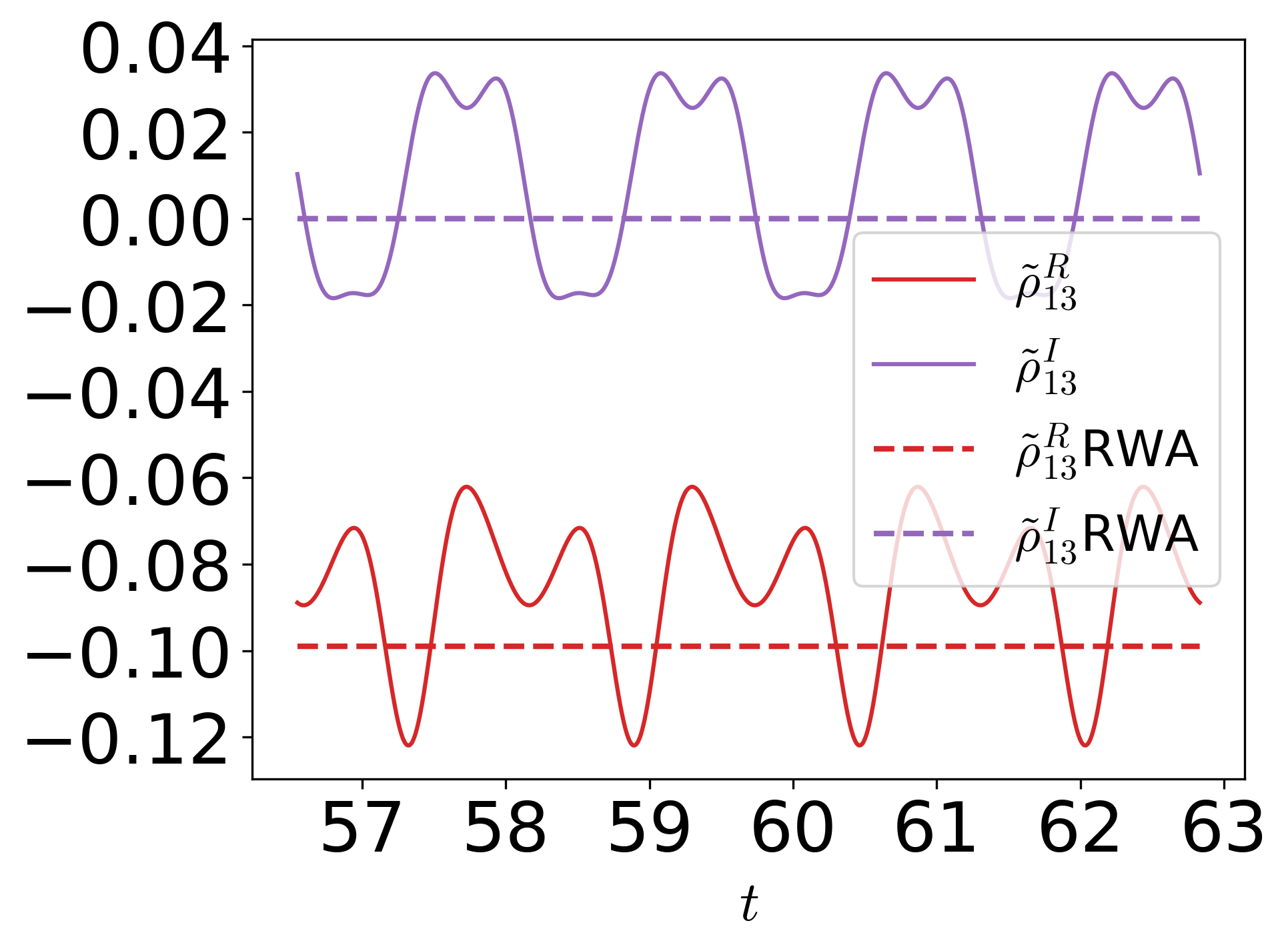
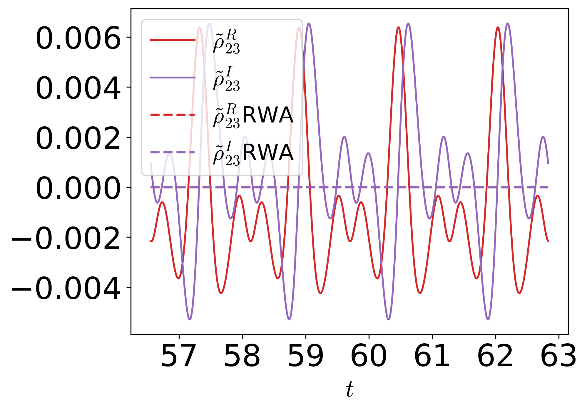
Figure 2 shows results for the case A-1 in Table LABEL:table-1, which corresponds to a representative example of EIT with perfect resonance but without the effects of bath. Results for both the full Hamiltonian and RWA are shown. We use to represent the off-diagonal elements in RWF (see Appendix A). Although the two results are qualitatively similar, there are substantial quantitative differences between their time dependences. In particular, the differences in the diagonal component of the density operator , imaginary parts of the off-diagonal elements, and , and the real part of the off-diagonal element, , are significant.
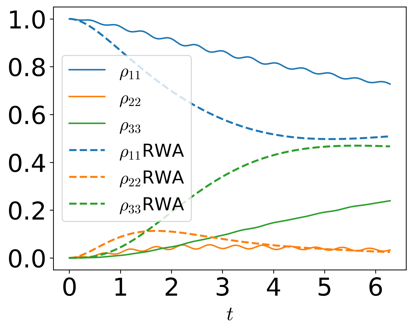
Figure 3 shows results for the case A-II in Table LABEL:table-1, for which EIT is observed with full resonance condition in the presence of photonic bath. The density operator in this case is governed by Eq. (5). Overall, the presence of bath significantly dampens coherent behavior and reduces the discrepancies between the results for the full and RWA Hamiltonians, but significant differences between the two can still be seen in all matrix elements of the system density operator. In particular, the differences between the two off-diagonal components of the density operator are substantial, and the imaginary parts of off-diagonal components are even qualitatively different.
We conducted similar calculations for cases B-I and B-II, for which both control and probe fields are weak and thus RWA is expected to work well, and also for cases C-I and C-II corresponding to a very strong control field. Detailed results of the time evolution of density operators for these cases are provided in Figs. S1-S7 in the SI.
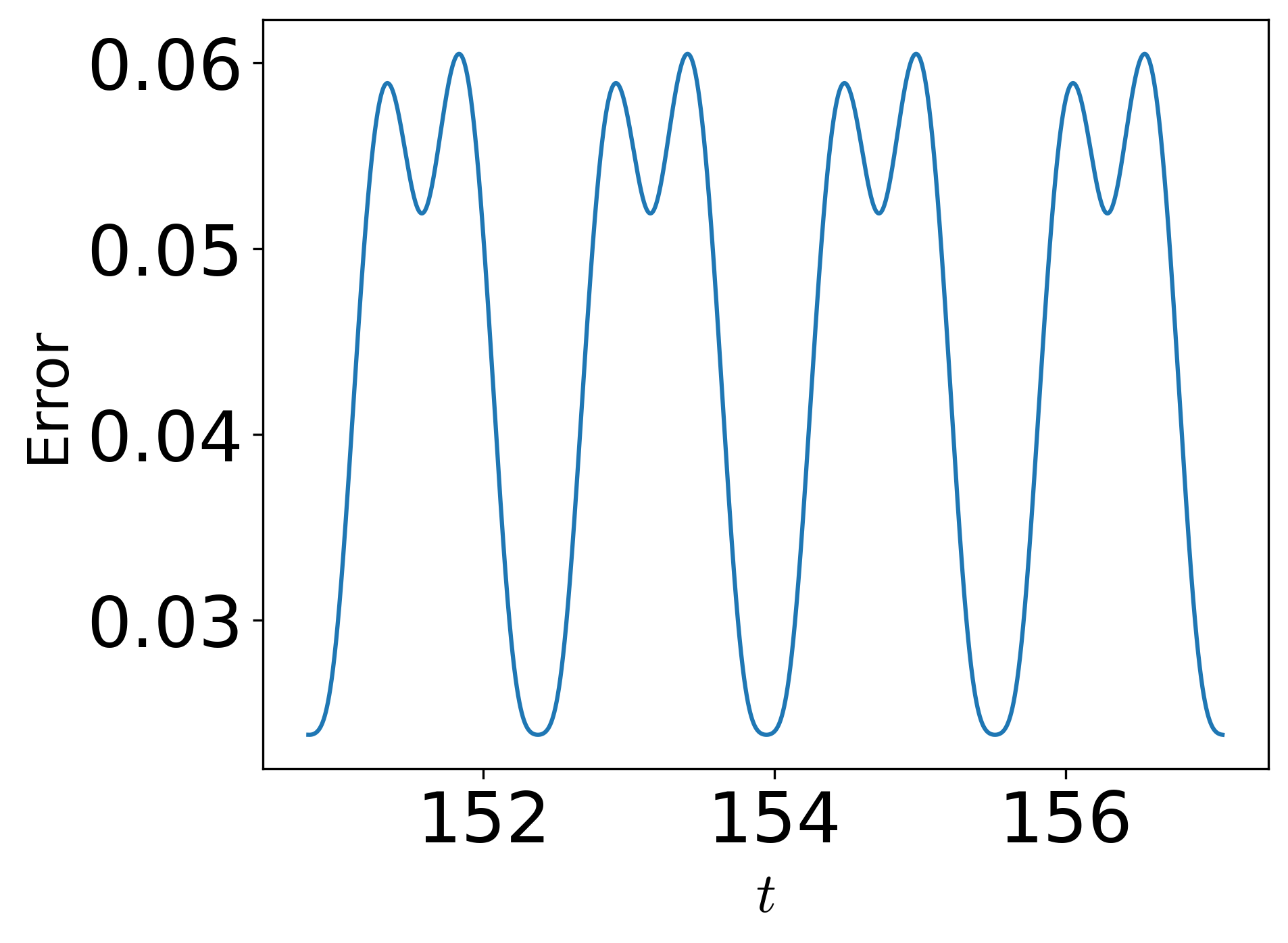
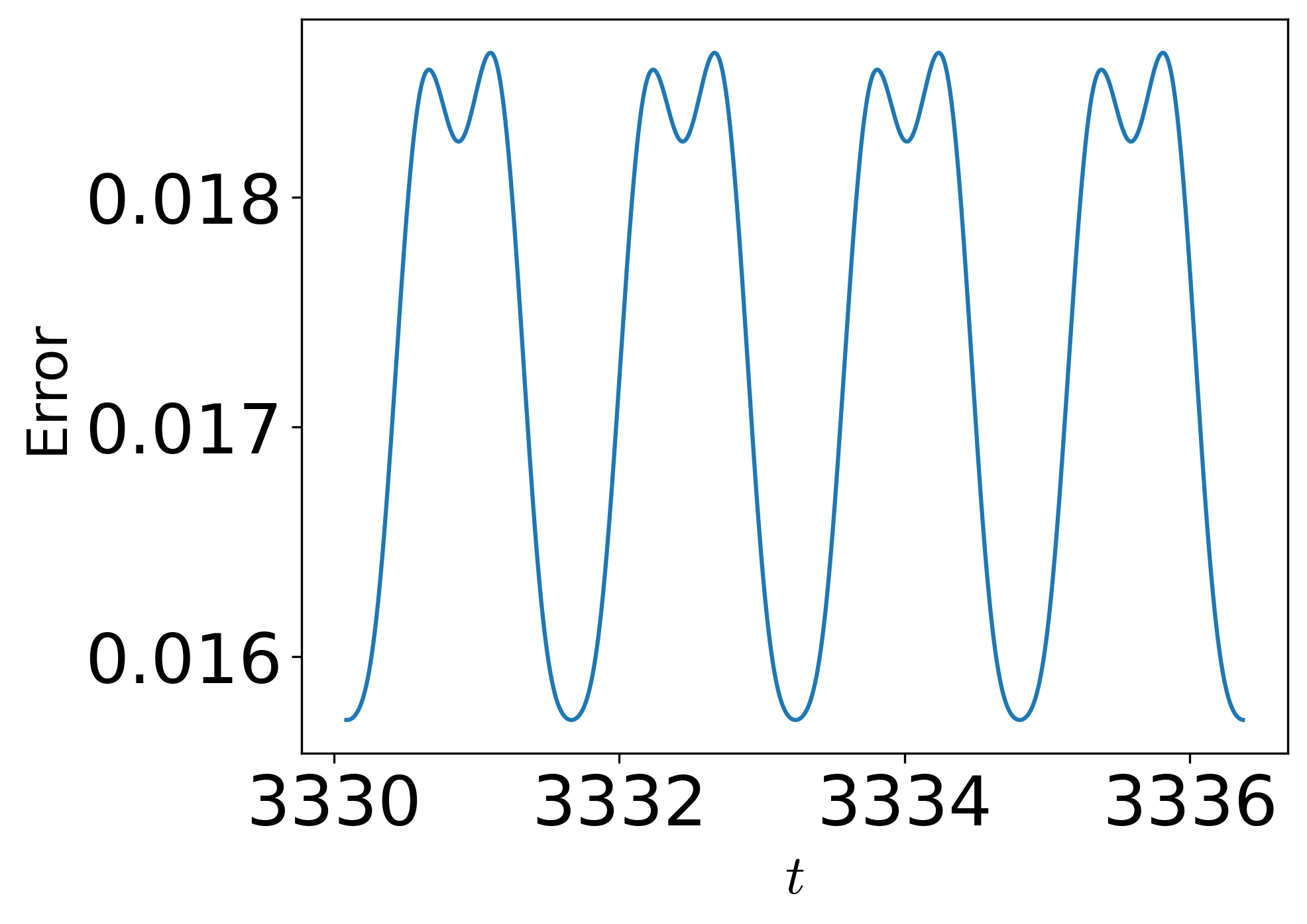
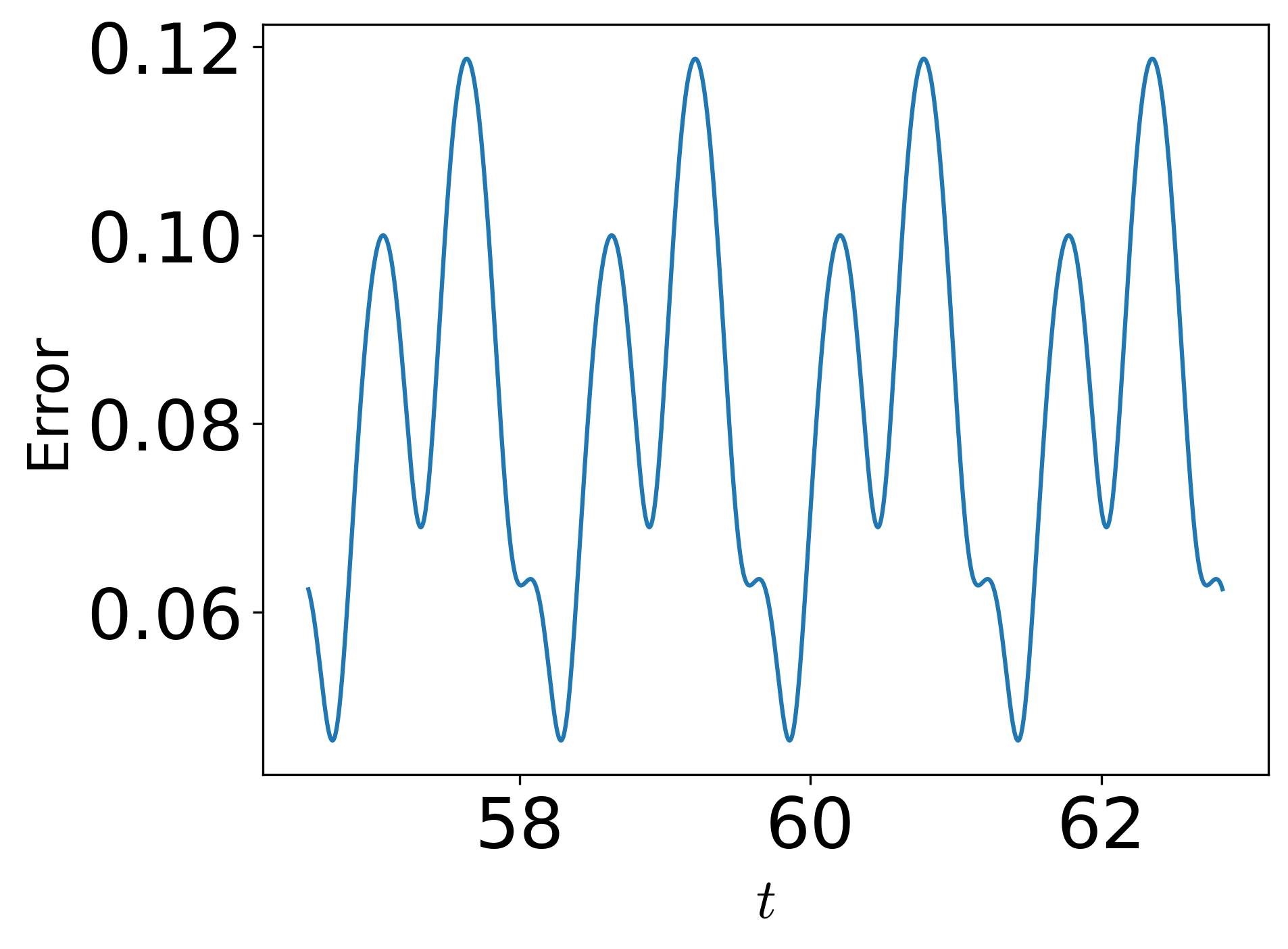
Figure 4 shows errors calculated according to Eq. (13) for all six cases during the initial dynamics. As expected, the errors for open system quantum dynamics are smaller than those for closed system dynamics since the environmental dissipation in the former cases mitigate oscillatory dynamics. The errors for cases B-I and B-II, which correspond to weak control and probe fields, are smaller than those for cases A-I and A-II. The cases for strong control field only, C-I and C-II, exhibit rapid initial growth of error when compared to the weak field cases, but then reach steady state values that are comparable to them. These results indicate that the errors of RWA are large particularly when both the control and probe field strengths are comparable. Figure S8 in SI shows errors in the long time limits for the three open system quantum dynamics, which confirm these assessments in the presence of bath.
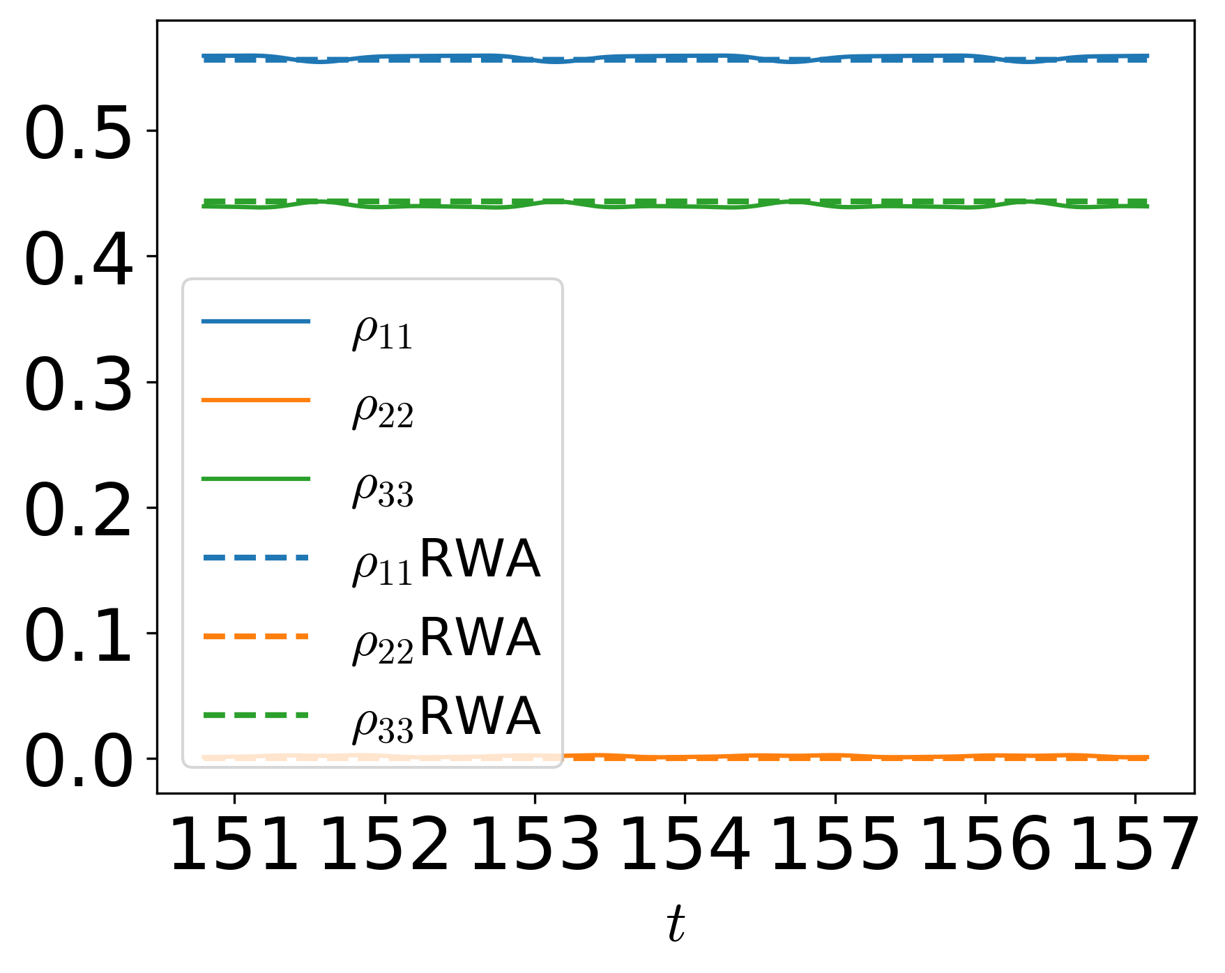
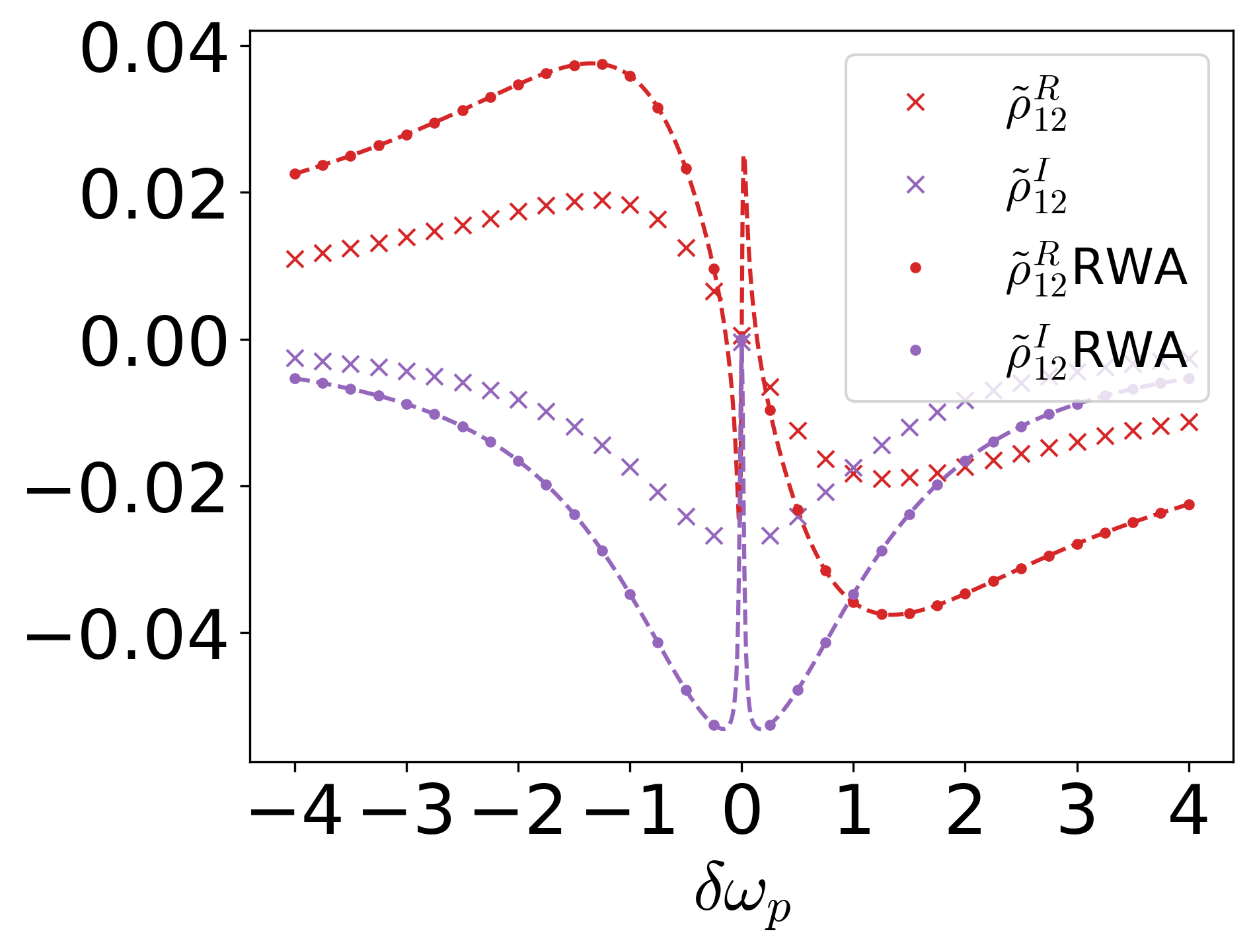
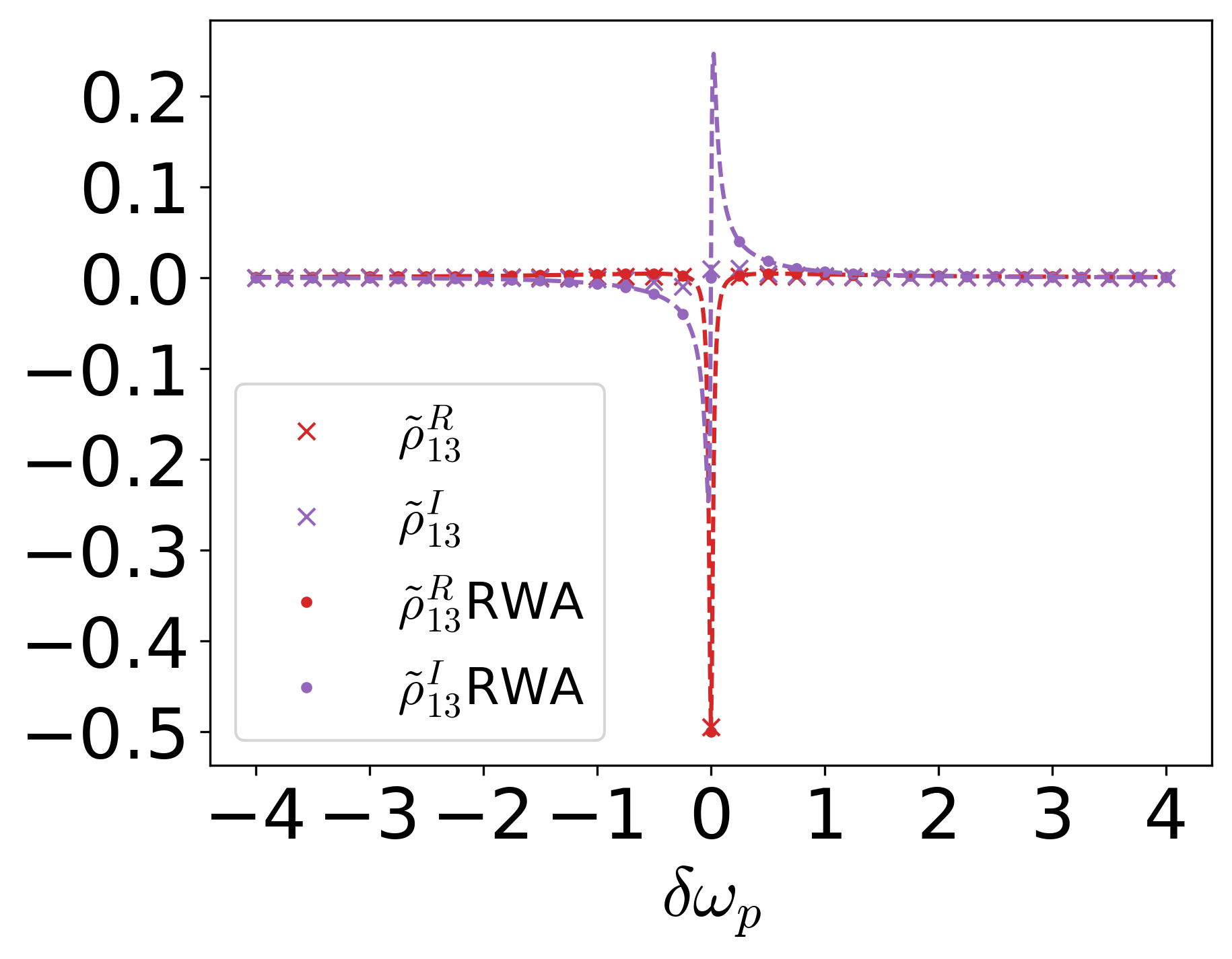
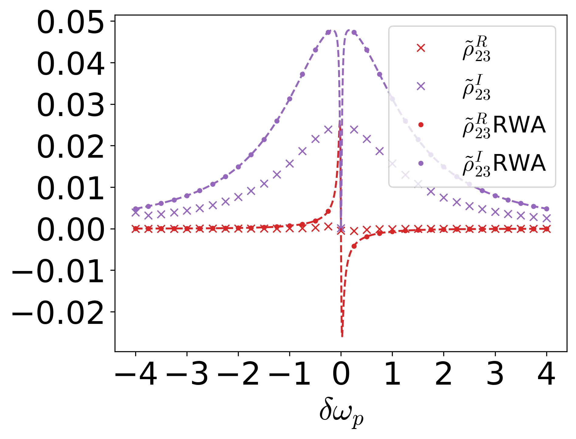
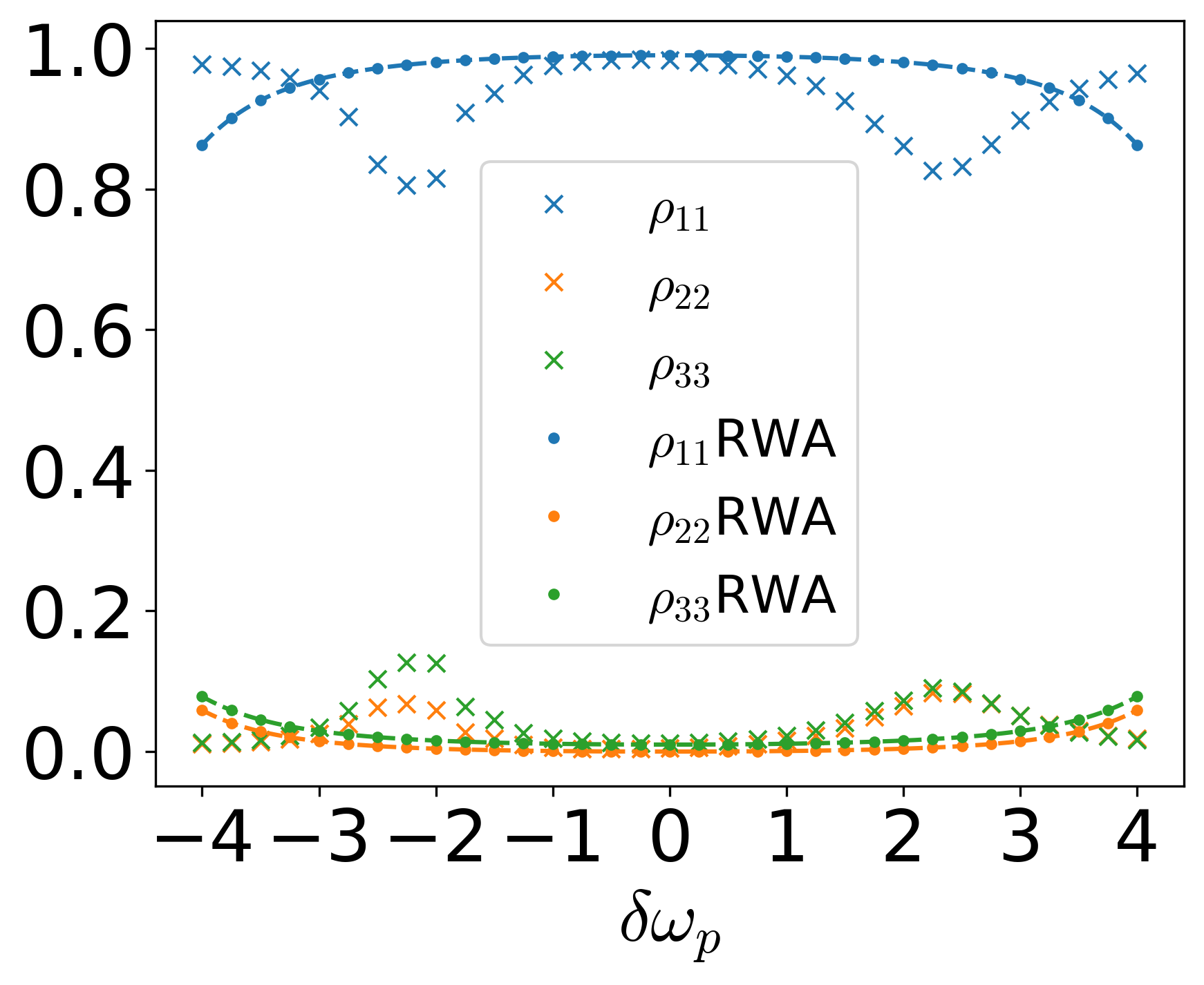
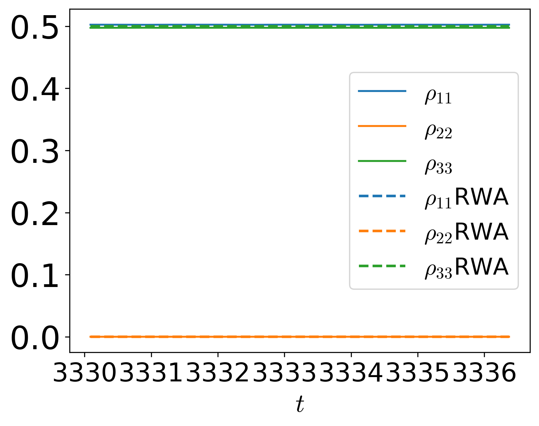
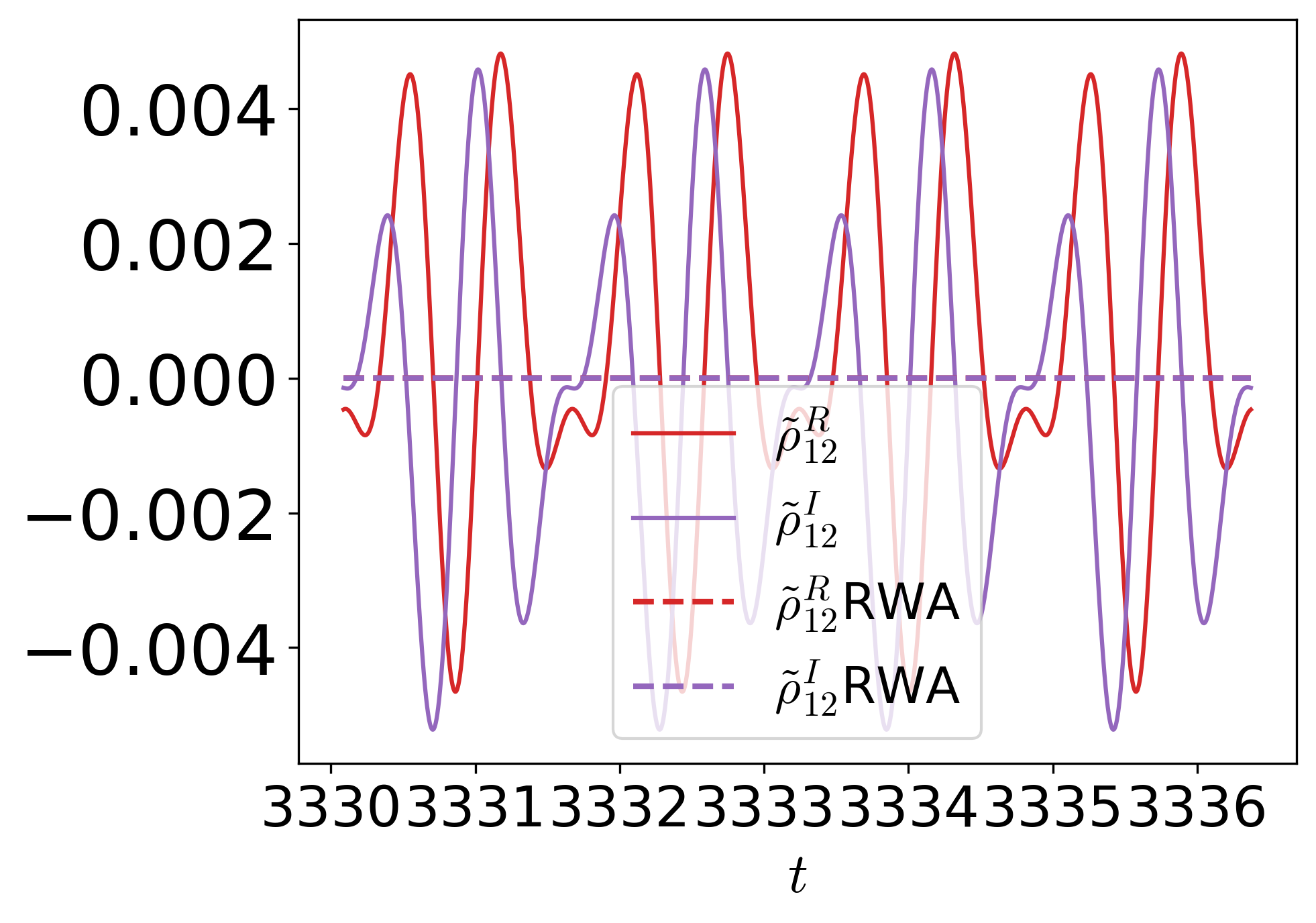
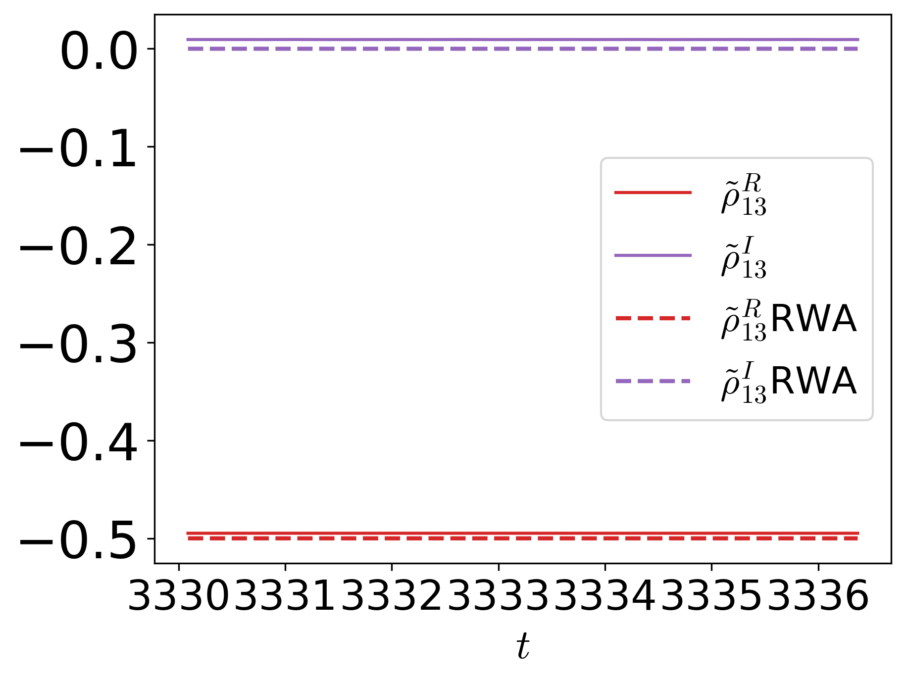
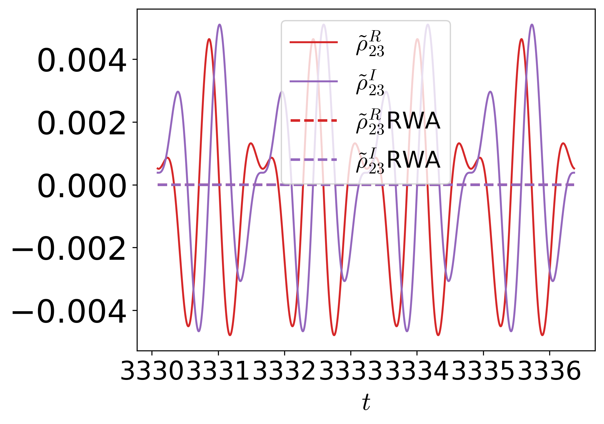
Figure 5 shows results again for the case A-II of Table I in the long time limit. The diagonal components of the density operator for RWA are in good agreement with those for the exact Hamiltonian. However, small discrepancies can still be seen in the off-diagonal components. This has significant implications for EIT, where the group velocity of probe radiation is determined from the off-diagonal elements of the density operator. We thus considered this issue in more detail by varying the value of around the resonance condition as described below.
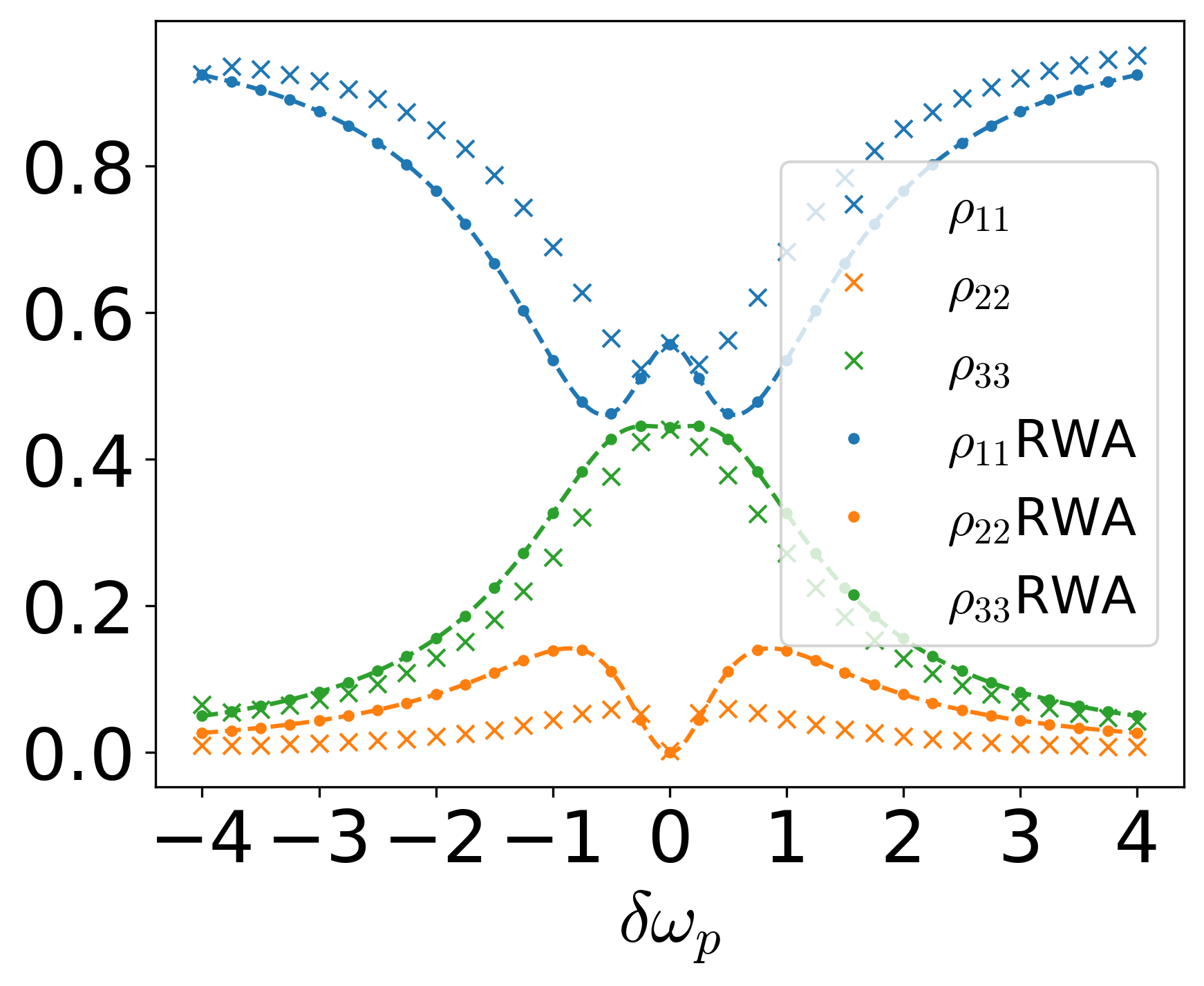
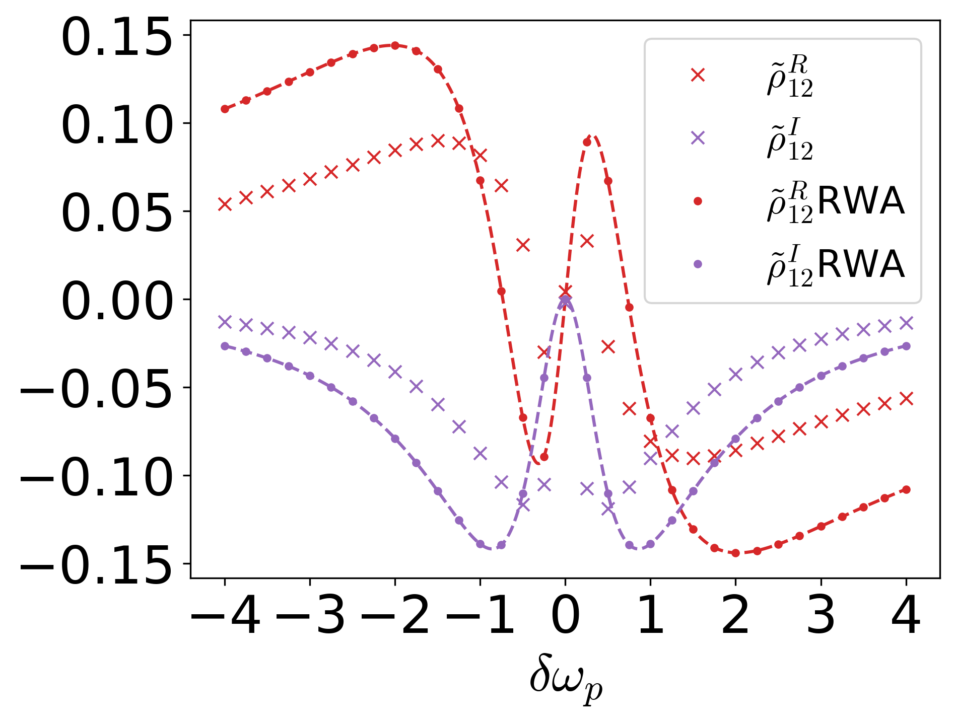
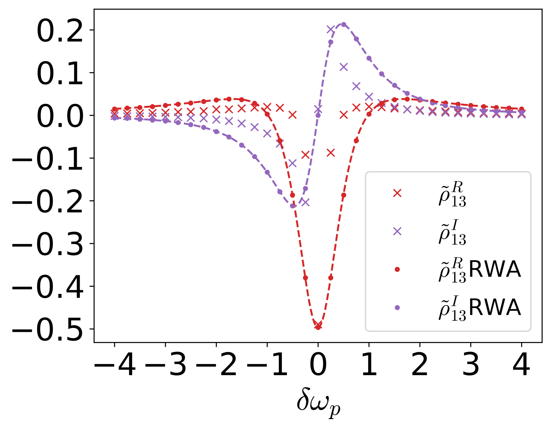
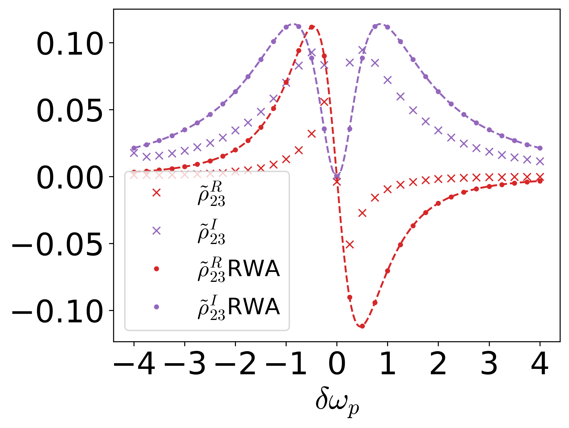
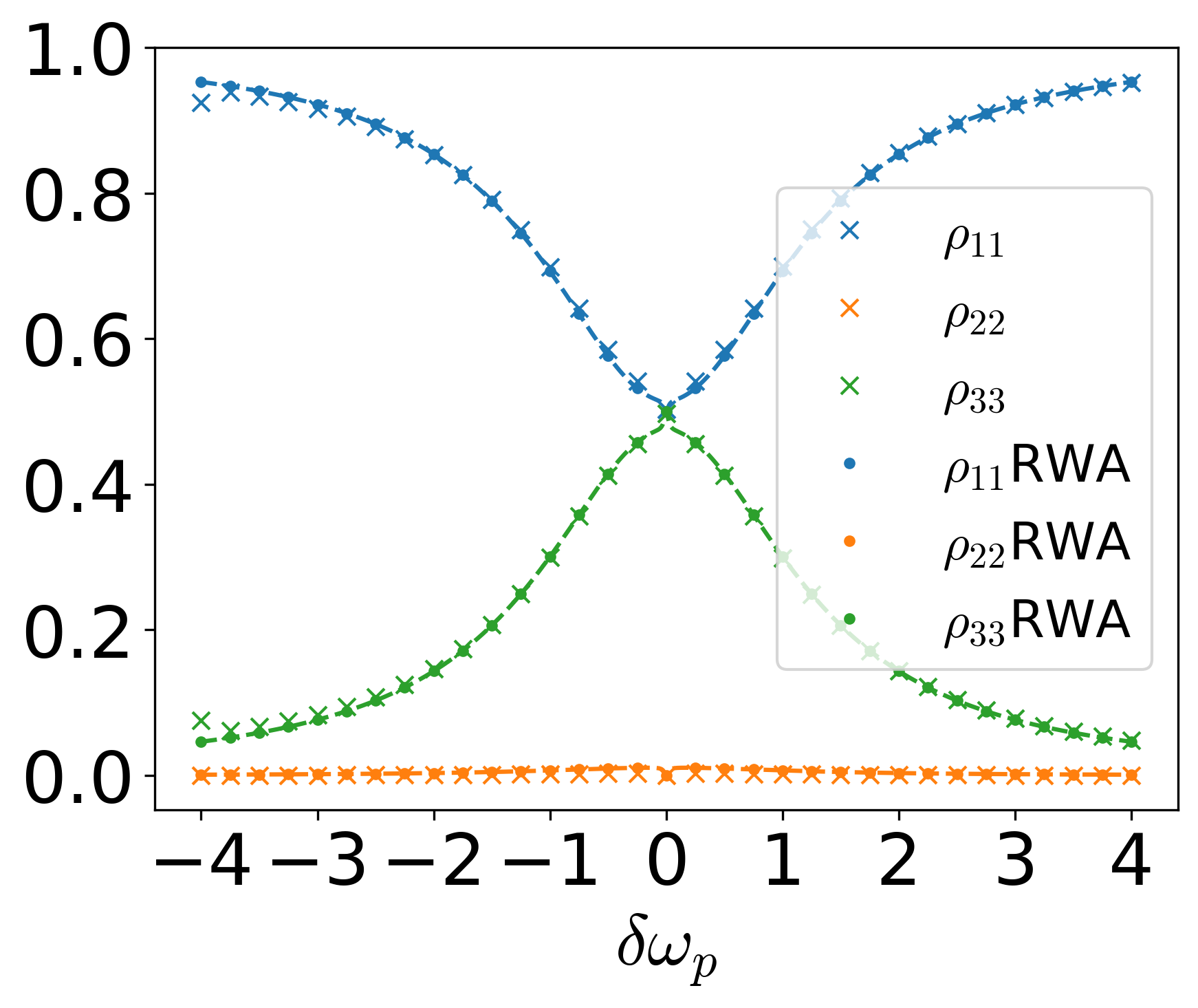
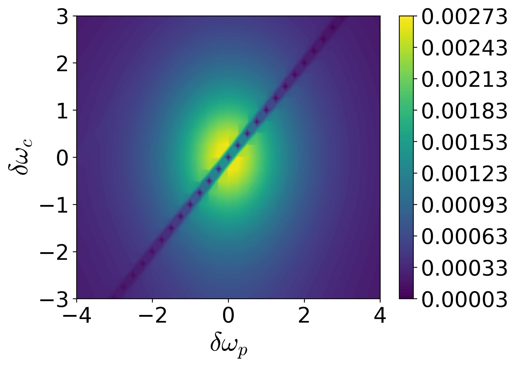
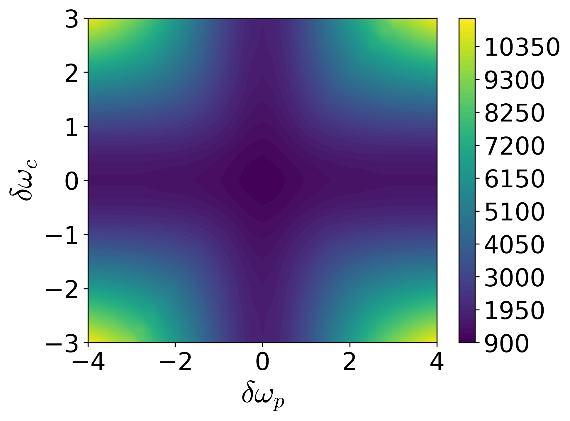
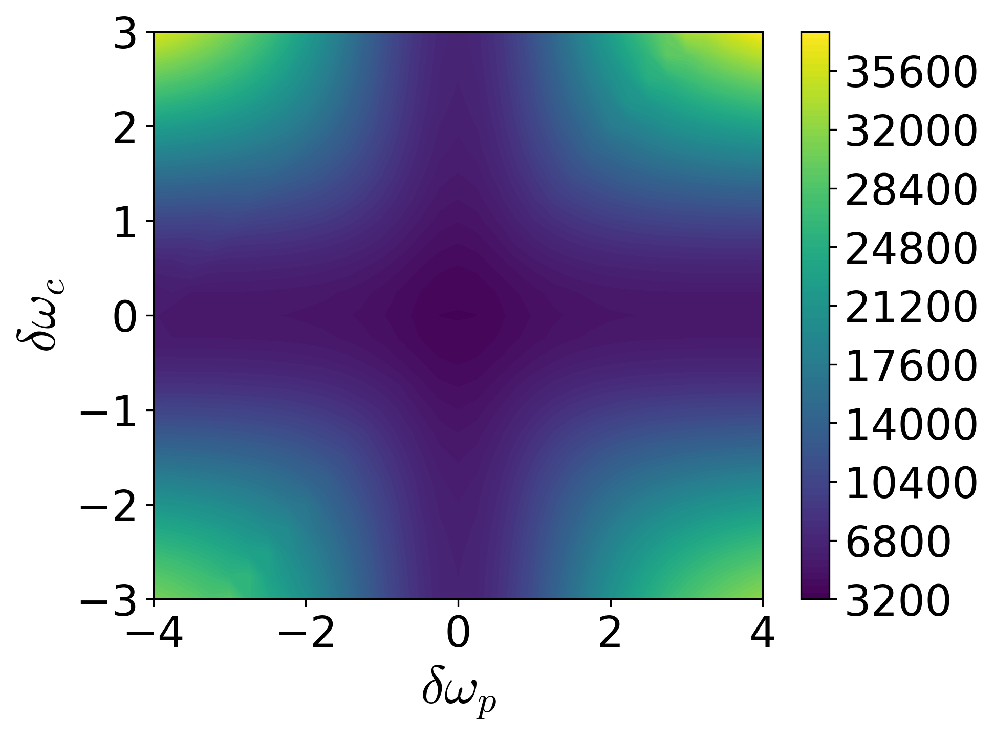
We conducted calculations for the long time limit for values of from 2 to 10 in increments of 0.25. For all of these cases, can be used. Once we have conducted the long time dynamics, we then calculated the average steady-state values of the system density operator matrix elements by integrating their time dependent values over an interval of with the trapezoid rule. The results are shown in Fig. 6. While the diagonal components of the steady state density operators for full and RWA Hamiltonians agree qualitatively, there are noticeable differences between them. For off-diagonal components, larger discrepancies can be seen. In particular, for the real parts of the off-diagonal elements, and , qualitative differences remain significant.
(a) (b)
(c) (d)
(a) (b)
(c) (d)
Although the steady state limit of the density operator within RWA becomes quite accurate especially for the case B, where both control and probe fields are weak, we find nonnegligible differences in the time it takes for the steady state value to be reached. This convergence rate can be vital in applications such as experimental realizations of qubits, which slowly lose coherences over time due to interactions with the environments. As an example, see Fig. S3 in SI. For this case (case B-II of Table LABEL:table-1), even after the results of RWA have converged, those for the full Hamiltonian have not reached steady state values yet.
For both cases of B-II and C-II, we also conducted additional calculations for non-resonant values of as was done for Fig. 6. The resulting patterns of different elements of the density operator are shown in Figs. 7 and 8. For the case B-II, Fig. 7 shows that most results for RWA agree well with those for the full Hamiltonian. However, there are about a factor of two differences for the off-diagonal elements and . Figure 8 shows significant qualitative differences between the two density operators for the case C-II, which confirms the unreliability of RWA for strong control fields.
(a) (b)
(c) (d)
(a) (b)
(c) (d)
(a) (b)

(c) (d)
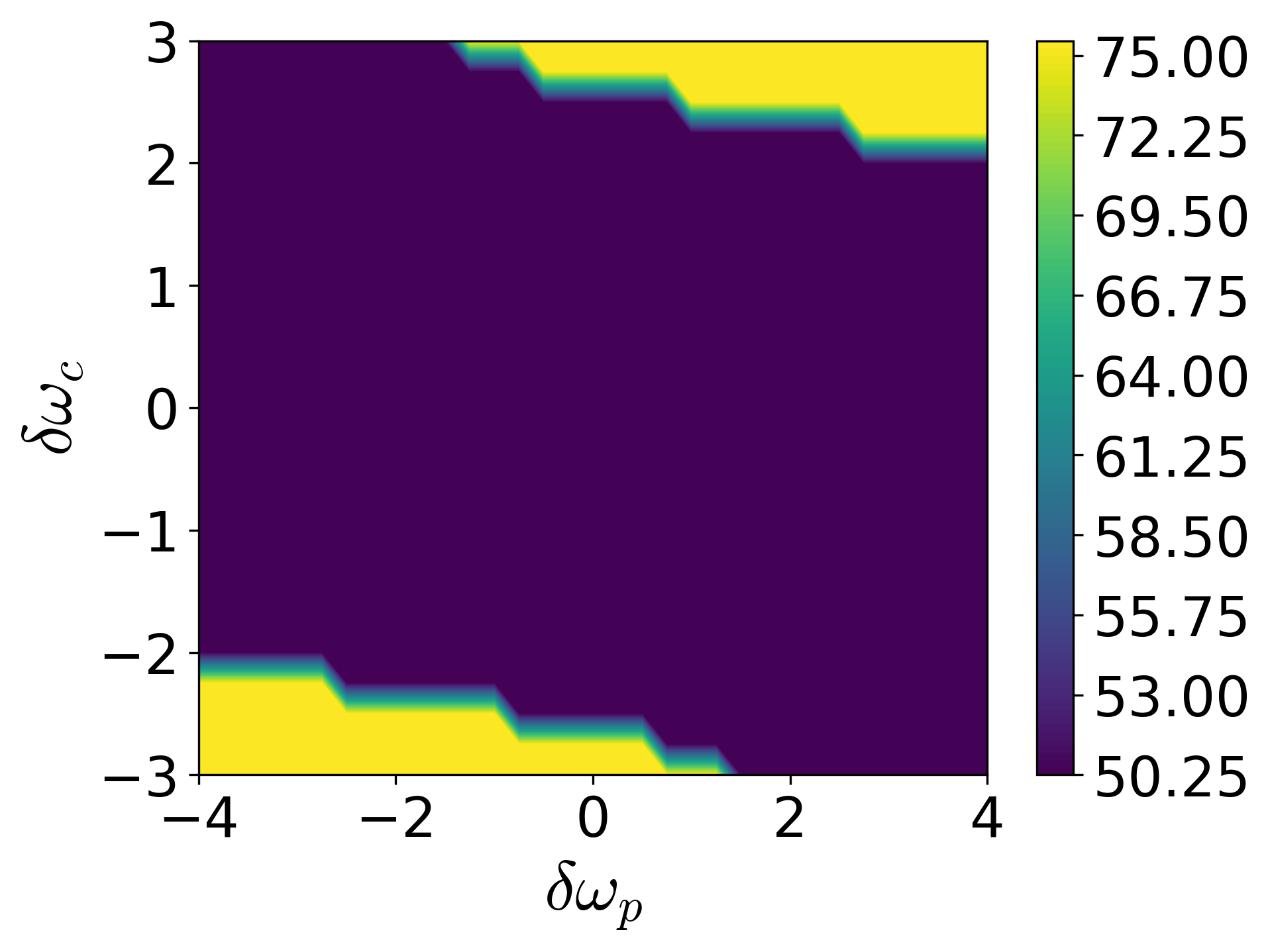
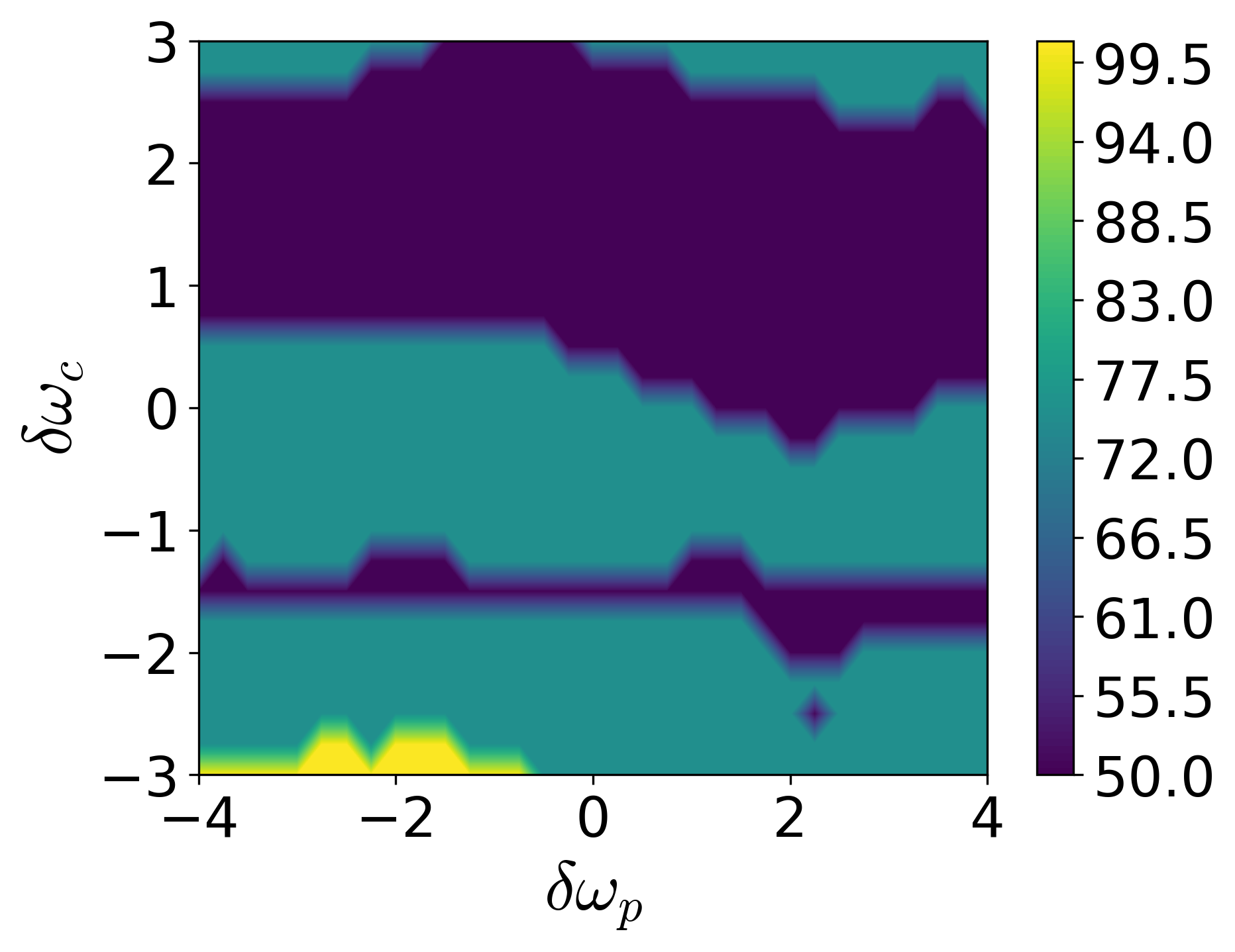
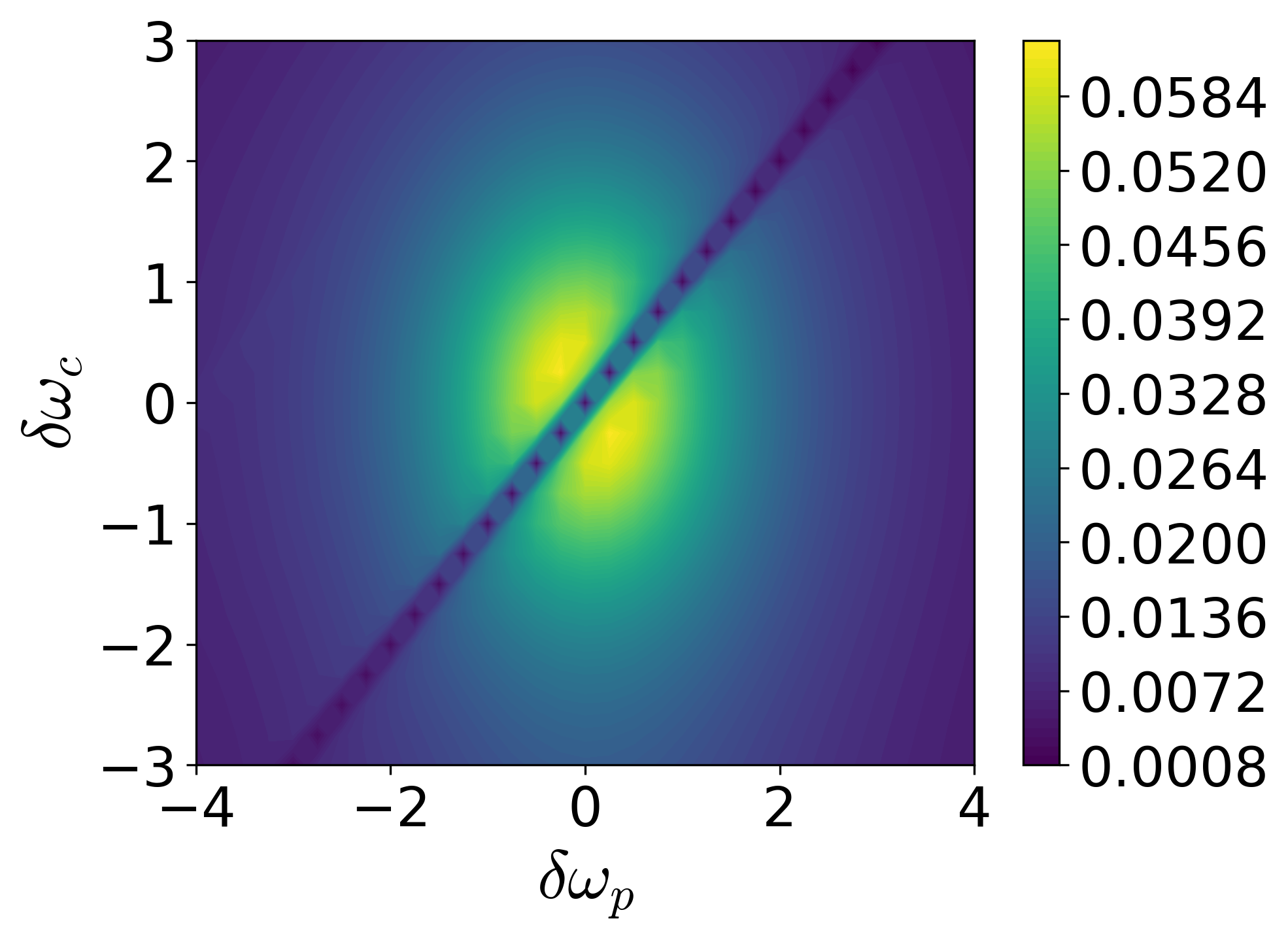
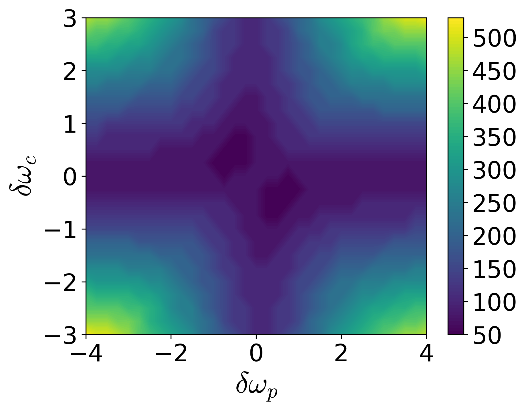
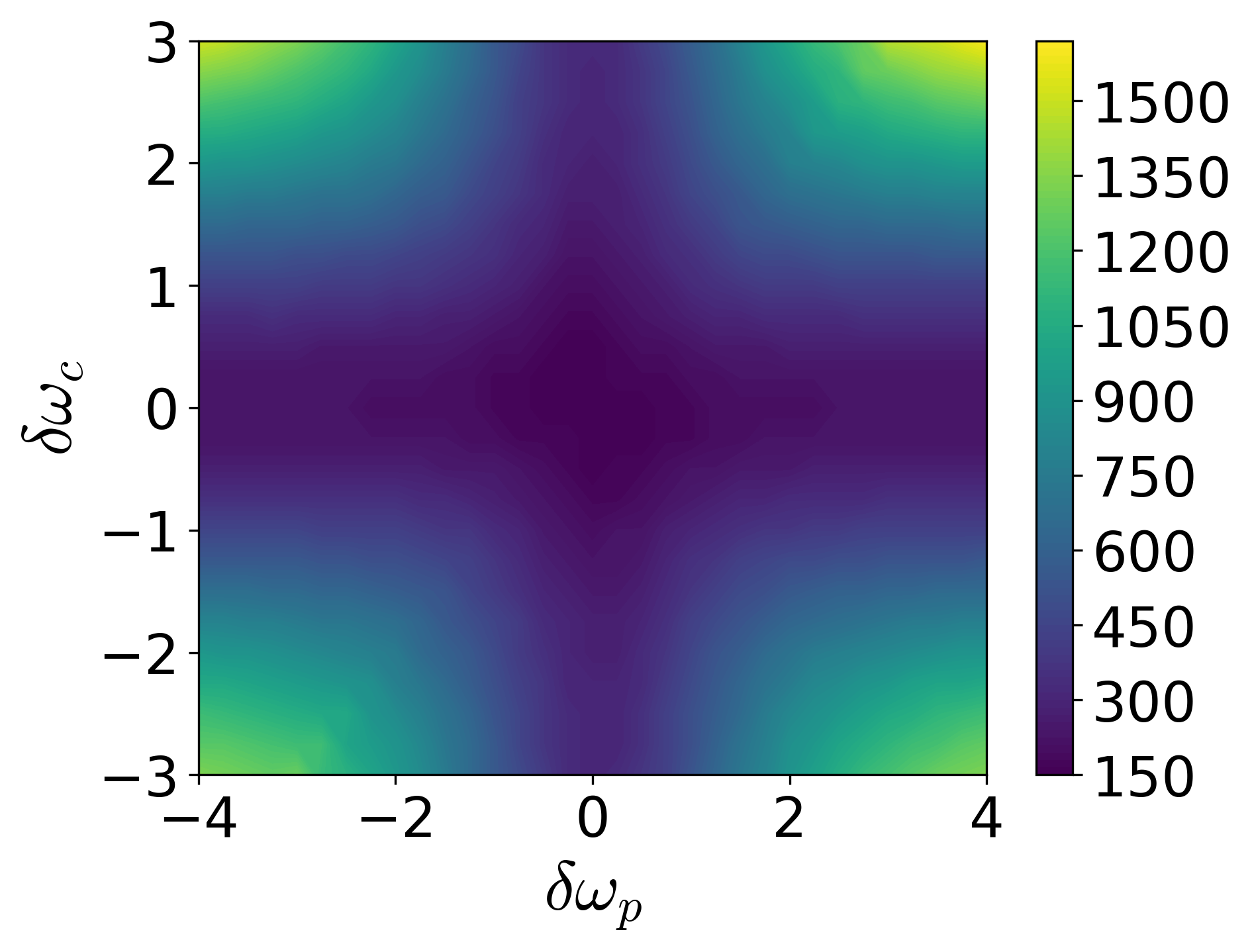
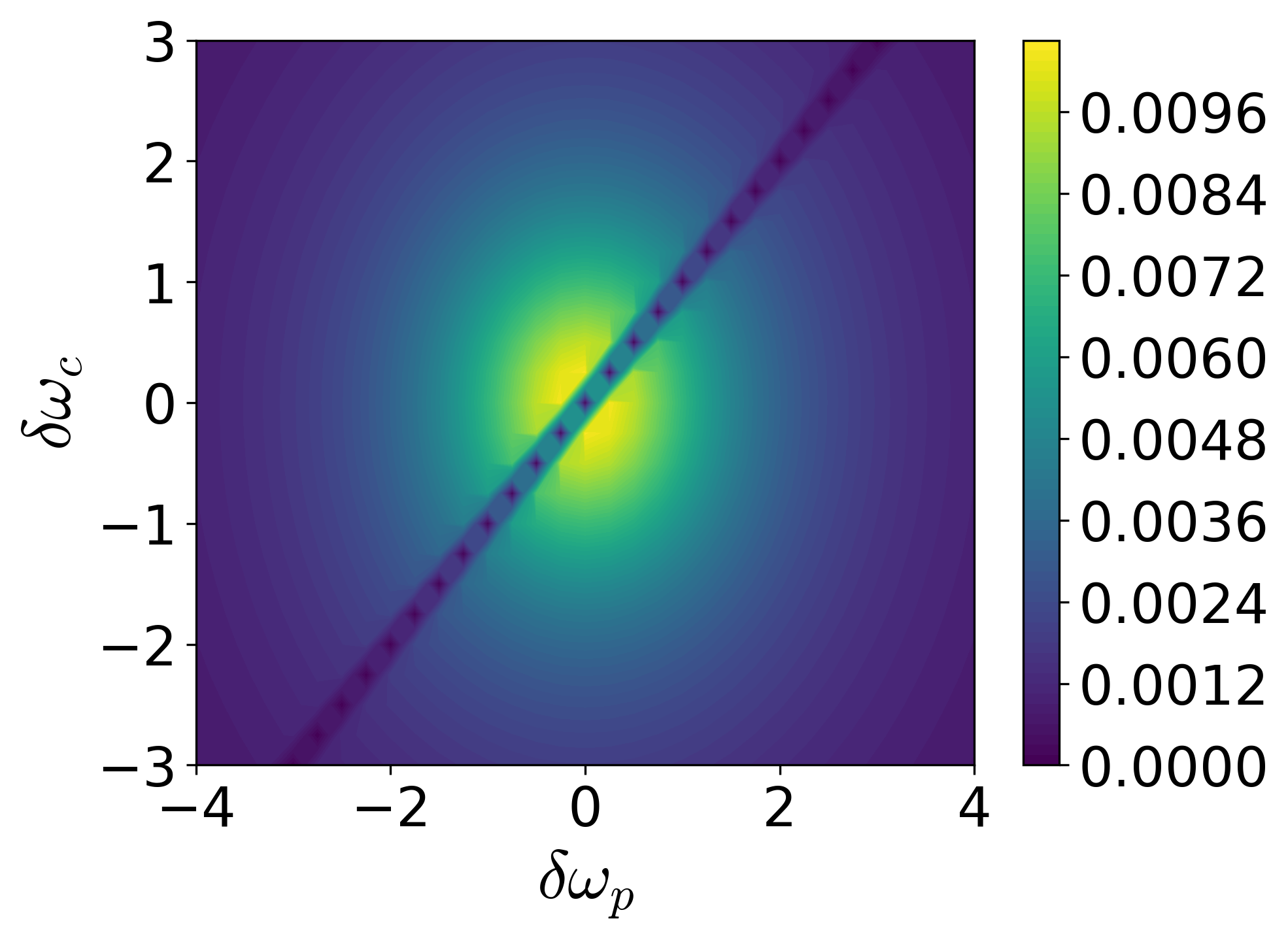
Note that results presented so far have not covered some interesting parameter regimes, such as the TPR with a non-zero detuning (), for which the phenomenon of CPT can still be observed. In recent works,[28, 29] these modified detunings were used in order to avoid transitions to an unwanted level, [28] and to swap populations of the two lower-lying states.[29] Figures 9-11 cover these cases and other parameter regimes by using and .
We notice that, even though the detuning case produces CPT, the time required to reach zero population in state increases as the absolute value of the detuning increases. This effect is seen for results of RWA Hamiltonian but is more pronounced for the dynamics resulting from the full radiation Hamiltonian. Figures 9-11 show that the RWA in general overestimates the population in state 2, underestimates the amount of time required to reach the steady state. Comparison of these figures show that the time to reach the steady state is largest for B-II, and smallest for C-II (B-II A-II C-II). This ordering corresponds directly with the amplitude of the pulses (, ). In all three cases, it is seen that there is no population in the excited state in the steady state limit under TPR conditions (the main diagonal in panels (a) and (b)). This explains why TPR is a requirement for stimulated Raman adiabatic passage (STIRAP),[30] which aims to transfer population from state to state without significantly populating the excited state. We also note that the shapes of Figs. 9 and 10 appear to be the inverse of Fig. 9 in Martin et al.,[31] which shows efficiency of the STIRAP process as a function and , using experimental data.
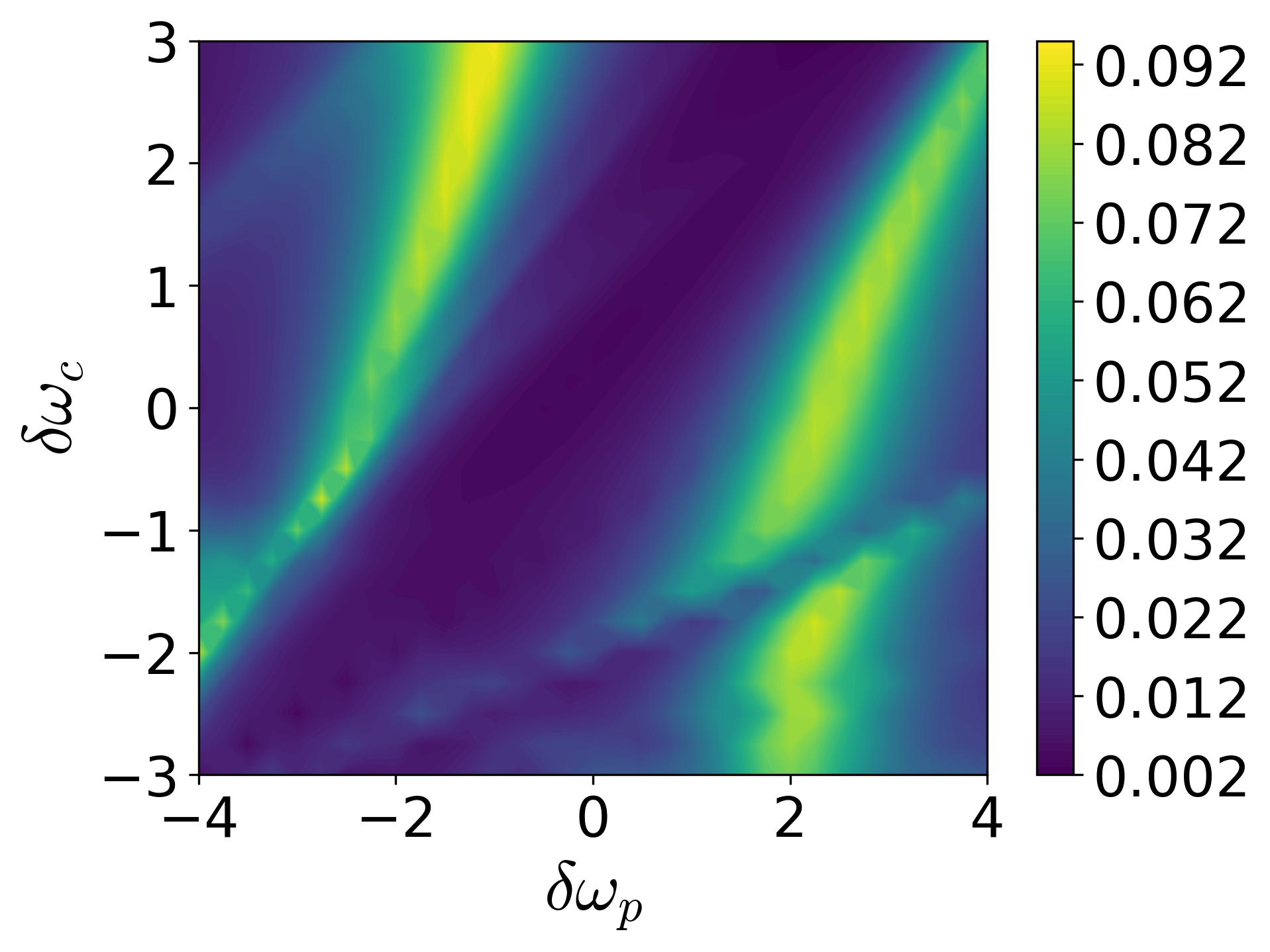
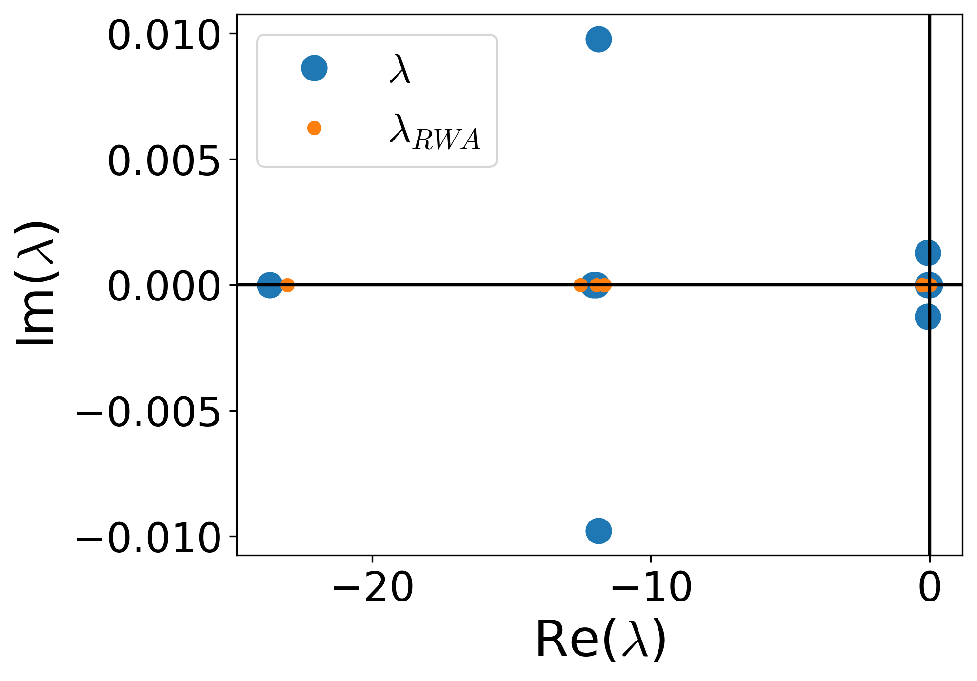
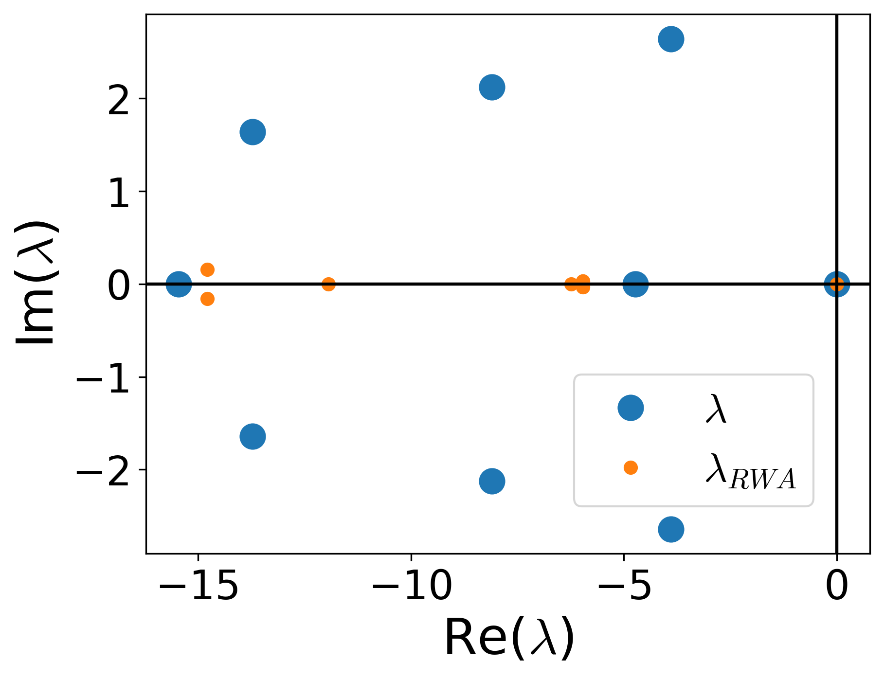
The difference in the dynamical behavior as described above can also be explained in terms of the eigenvalues of or time-dependent eigenvalues of . From the former, the time to reach the steady state can be found by determining the spectral gap , which is determined by the eigenvalue with real part closest to zero. [32] Plots of the latter shown in Fig. 12 provide interesting dynamical information such as avoided crossings. Note also the symmetry with respect to the axis of , which is expected for a CPTP map.
(a)

(b)
(c)
VI Conclusion
RWA for the matter-radiation interaction Hamiltonian has been used widely due to its convenience and conceptual clarity, and is indeed well established as an accurate approximation for conventional spectroscopy measurements in the weak field limit. However, its accuracy for matter-radiation interactions involving multiple pulses beyond the weak field limit has rarely been tested. Considering recent experimental advances in nonlinear spectroscopy, QC, and QS and the need for more accurate calculation methods of optical signals involved, the methods and outcomes presented in this work have significant implications.
Results of our calculation for a prototypical -system are consistent with the general notion that RWA becomes reliable in the weak field and steady state limits. However, even for this case, the early behavior of the nonequilbrium dynamics and the values of off-diagonal matrix elements of the density operator based on RWA were different from those of the full Hamiltonian in nontrivial manner. For moderately strong control and probe fields and for a very strong control field we have tested, we find some of the results based on RWA Hamiltonian exhibit quantitatively significant or even qualitative differences from those of full Hamiltonian. These results indicate the danger of drawing too much conclusion from results of RWA Hamiltonian and motivate seeking accurate dynamics methods for multi-level systems driven by multiple pulses.
Another important aspect of our work is the extension and test of ME to the Liouville space for both closed and open system dynamics. Although we have used the 6th order approximation[19] in order to ensure as accurate calculation as possible, we confirmed that the performance of our simplest 4th order approximation[19] is practically similar. In SI, we provide explicit expressions for the 4th order approximations in the Liouville space, whereas the 6th order approximation is offered only in the form of python code that we make public.222https://github.com/TanerTure/LambdaRWACode
The stability of our ME based numerical method for the non-Hermitian dynamics (e.g. Figs. 3 and 5) is noteworthy and warrants further discussion. The trace of unity is maintained with only negligible deviations (on the order of in the worst case) due to numerical error, even in the long-time limit. This suggests that, for the time-dependent system Hamiltonian with time-independent Lindblad dissipative terms as in Eq. (6), the ME truncated at any order produces a trace preserving map. In fact, we find numerically that it produces a completely positive trace preserving map (CPTP). CPTP maps not only guarantee that the trace is maintained, but that the resulting density operator is physical even if it only describes a subsystem. An analytical proof for the closed system case is shown in Appendix D. For the open system case, the CPTP map is produced because of the small step size, which ensures that the first order term of the ME is larger than the subsequent terms. It is easily proven that the first order term of the Magnus expansion defines a CPTP map, while it has been shown that higher order terms contribute to breaking the complete positivity.[33]
As a further extension of this work, one can imagine using the nearly exact numerical time evolution provided here to produce large quantities of data for a deep learning or reinforcement learning algorithm, with the goal of finding improved pathways (beyond well-known shortcuts to adiabaticity methods) to produce the desired population transfer in a short amount of time, that is also relatively insensitive to experimental parameters. Code for ME is currently being optimized for this purpose.
Acknowledgements.
S.J.J. acknowledges major support of this research from the US Department of Energy, Office of Sciences, Office of Basic Energy Sciences (DE-SC0021413) and partial support during the initial stage of this research from the National Science Foundation (CHE-1900170). S.J.J. also acknowledges support from Korea Institute for Advanced Study through its KIAS Scholar program for the visit during summer.Appendix A Closed system dynamics in the rotating wave frame (RWF)
The RWF is defined by the following time dependent unitary operator:
| (14) |
Thus, for a state , the corresponding state in the RWF is defined as
| (15) |
Given that the time evolution of is governed by , which is the sum of Eqs. (1) and (4), the time evolution equation for is
| (16) | |||||
where
| (17) | |||||
For a density operator in the original frame, we can also define the density operator in the RWF as follows:
| (18) |
The diagonal components of are the same as those of . On the other hand, the off-diagonal components are related by
| (19) | |||||
| (20) | |||||
| (21) |
and complex conjugates of the above relations.
The time evolution operator for can be found easily by diagonalizing , which is time independent. Assuming that , , and , the matrix representation of in the basis of , , and is given by
| (22) |
Appendix B Solution of closed system dynamics using RWA at the TPR conditions
Diagonalizing Eq. (22) involves solving a cubic equation for the eigenvalues, which can be quite cumbersome. However, under TPR conditions with zero detuning, the resulting cubic equation is simpler to solve because zero is a root of the characteristic polynomial. The other two eigenvalues are given by and , where .[16] Using these values and their associated eigenvectors, we find that the time evolution operator for is given by
| (23) | |||||
Employing the above expression, can be calculated for the initial condition . The resulting matrix expression in the basis of , , and is
| (24) |
It is easily verified that the analytical solution defined above satisfies and . In addition, taking produces a solution consistent with previous analytical results for the population.[16] The exact result is indistinguishable from the numerical results in Fig. 2 and Figs. S1 and S5 in the SI, and were therefore not plotted. The offdiagonal elements of the above density operator elements in the rotating frame can be expressed in terms of those in the original frame by using Eqs. (19)-(21) and their complex conjugates.
Appendix C Liouville-space transformation
Liouville representation[34, 15, 26] offers a convenient way to treat time evolution of density operators by representing them as vectors (or superkets) and have long been used for open system quantum dynamics and spectroscopy. It is important to note that the mapping from an operator in the Hilbert space to a superket in the Liouville space is not unique and thus care should be taken to maintain a consistent definition. We here employ the approach described recently by Gyamfi.[26] According to this prescription, the mapping from a Hilbert space to the corresponding Liouville space is implemented by the following mapping that flips the bra side of an arbitrary outer product and creates a direct product as follows:
| (25) |
where is the complex conjugate of . According to this mapping, the density operator is mapped to a superket as follows:
| (26) |
Then, all the operator identities in the Hilbert space can be mapped[26] uniquely into the Liouville space employing the mapping defined by Eq. (25). For the description of the time evolution of the density operator, the main relationship needed is the following mapping of triple product of operators (in the Hilbert space):[26]
| (27) |
where is a super-operator acting on the superket (in the Liouville space) from the lefthand side.
Appendix D Proof that truncated Magnus expansion produces a completely positive trace preserving (CPTP) map
Using the same Liouville space notation as in Appendix C, a map is CPTP if and only if it can be written in the following form:[35]
| (28) |
where is called the Krauss operator and sum of these must be the identity operator in the system Hilbert space as follows:
| (29) |
Application of the Magnus expansion truncated at the th order to the closed system dynamics in Eq. (9) yields
where is a functional of superoperators in the exponent of Eq. (9), consisting of iterated integrals and commutators (for precise definitions, see Ref. 19) . However, note that because , it becomes possible to separate the exponent in Eq. (D) into two terms:
| (30) |
where and was used. Now, multiplying and using the fact that , Eq. (30) can be expressed as
which clearly has the form of Eq. (28) with .
Since is guaranteed to be unitary at any finite order, Eq. (29) is also satisfied for any finite order approximation for the ME. This proof shows that the Hilbert space property of the ME (guaranteed unitary operator at any order of truncation) translates into the corresponding Liouville space property of CPTP map for Hermitian dynamics. Also in analogy with the Hilbert space situation, propagators based on time-dependent perturbation theory fail to be CPTP maps; they clearly violate Eq. (29). Note that the above proof for closed system dynamics remains true even with RWA.
References
- [1] M. Shapiro and P. Brumer, Quantum control of molecular processes, 2nd edition (Wiley-VCH, Weinheim, 2013).
- [2] K. Bergmann, H. Theuer, and B. W. Shore, Rev. Mod. Phys. 70, 1003 (1998).
- [3] G. S. Vasilev, A. Kuhn, and N. V. Vitanov, Phys. Rev. A 80, 013417 (2009).
- [4] H. Gray, R. Whitley, and C. Stroud, Opt. Lett. 3, 218 (1978).
- [5] K.-M. C. Fu et al., Phys. Rev. Lett. 95, 183601 (2005).
- [6] K. J. Boller, A. Imamoglu, and S. E. Harris, Phys. Rev. Lett. 66, 2593 (1991).
- [7] M. Fleischhauer and M. D. Lukin, Phys. Rev. Lett. 65, 022314 (2002).
- [8] L. Ma, O. Slattery, and X. Tang, J. Opt. 19, 043001 (2017).
- [9] F. Carreño, O. G. Calderón, M. A. Antón, and I. Gonzalo, Phys. Rev. A 71, 063805 (2005).
- [10] A. A. Abdumalikov et al., Phys. Rev. Lett. 104, 193601 (2010).
- [11] D. Singh, S. J. Jang, and C. Hyeon, J. Phys. A: Math. Theor. 56, 015001 (2023).
- [12] C. L. Degen, F. Reinhard, and P. Capellaro, Rev. Mod. Phys. 89, 035002 (2017).
- [13] H. Zhang, G.-Q. Qin, X.-K. Song, and G.-L. Long, Opt. Express 29, 5358 (2021).
- [14] P. Rembold et al., AVS Quantum Sci. 2, 024701 (2020).
- [15] S. Mukamel, Principles of Nonlinear Spectroscopy (Oxford University Press, New York, 1995).
- [16] B. W. Shore, Manipulating quantum structures using laser pulses (Cambridge University Press, Cambridge, 2011).
- [17] G. Berlín and J. Aliga, J. Opt. B: Quantum Semiclass. 6, 231 (2004).
- [18] M. A. Jørgensen and M. A. Wubs., J. Phys. B: At. Mol. Opt. Phys. 55, 195401 (2022).
- [19] T. M. Ture and S. J. Jang, J. Phys. Chem. A 128, 2871 (2024).
- [20] We use a labeling convention of the -system states that are more commonly used for quantum control and quantum sensing.
- [21] D. Thirumalai, E. J. Buskin, and B. J. Berne, J. Chem. Phys. 79, 5063 (1983).
- [22] F. Casas, J. A. Oteo, and J. Ros, J. Phys. A Math. Gen. 34, 3379 (2001).
- [23] A. Eckardt and E. Anisimovas, New J. Phys. 17, 93039 (2015).
- [24] T. Kuwahara, T. Mori, and K. Saito, Ann. Phys. 367, 96 (2016).
- [25] A. Brinkmann, Concept Magn. Reson. A 45, e21414 (2016).
- [26] J. A. Gyamfi, Euro. J. Phys. 41, 63002 (2020).
- [27] I. I. Boradjiev and N. V. Vitanov, Phys. Rev. A 81, 053415 (2010).
- [28] A. Vezvaee et al., PRX Quantum 4, 30312 (2023).
- [29] G. T. Genov et al., J. Phys. B: At. Mol. Opt. Phys. 56, 54001 (2023).
- [30] N. V. Vitanov, A. A. Rangelov, B. W. Shore, and K. Bergmann, Rev. Mod. Phys. 89, 015006 (2017).
- [31] J. B. Martin, B. W. Shore, and K. Bermann, Phys. Rev. A 54, 1556 (1996).
- [32] V. V. Albert and L. Jiang, Phys. Rev. A 89, 22118 (2014).
- [33] K. Mizuta, , K. Takasan, and N. Kawakami, Phys. Rev. A 103, L020202 (2021).
- [34] U. Fano, in Lectures on the Many-body Problems (Academic Press, New York, 1964), pp. 217–239.
- [35] M.-D. Choi, Linear Algebra Appl. 10, 285 (1975).
- [36] https://github.com/TanerTure/LambdaRWACode.
Supporting Information: Application of Magnus expansion for the quantum dynamics of -systems under periodic driving and assessment of the rotating wave approximation
S1. Some numerical results for cases in Table I of main text
Some results of calculation for Cases B-I, B-II, C-I, and C-II in Table I of the main text are provided here. Errors of RWA for cases A-II, B-II, and C-II in the long time limit are also provided.
(a) (b)
(c) (d)
(a) (b)
(c) (d)
(a) (b)
(c) (d)
(a) (b)
(c) (d)
(a) (b)
(c) (d)
(a) (b)
(c) (d)
(a) (b)
(c) (d)
(a)
(b)
(c)
S2. Explicit terms for fourth-order Magnus Expansion propagator in Liouville space
From Eq. (10) in the main text, the propagator for the closed system dynamics is given by
| (S1) |
Using a recently derived fourth-order Magnus Expansion propagator, the time-evolution from to can be approximated as
| (S2) |
where denotes the commutator and the matrix is given by .
For the open system case,
| (S3) | |||||
where is explicitly defined in Eq. (11) of the main text. Then, the Magnus Expansion propagator becomes
| (S4) | |||||