A Fully Parameter-Free Second-Order Algorithm for Convex-Concave Minimax Problems with Optimal Iteration Complexity

Abstract

In this paper, we study second-order algorithms for the convex-concave minimax problem, which has attracted much attention in many fields such as machine learning in recent years. We propose a Lipschitz-free cubic regularization (LF-CR) algorithm for solving the convex-concave minimax optimization problem without knowing the Lipschitz constant. It can be shown that the iteration complexity of the LF-CR algorithm to obtain an $\epsilon$-optimal solution with respect to the restricted primal-dual gap is upper bounded by $\mathcal{O}(\frac{\rho\|z^{0}-z^{*}\|^{3}}{\epsilon})^{\frac{2}{3}}$, where $z^{0}=(x^{0},y^{0})$ is a pair of initial points, $z^{*}=(x^{*},y^{*})$ is a pair of optimal solutions, and $\rho$ is the Lipschitz constant. We further propose a fully parameter-free cubic regularization (FF-CR) algorithm that does not require any parameters of the problem, including the Lipschitz constant and the upper bound of the distance from the initial point to the optimal solution. We also prove that the iteration complexity of the FF-CR algorithm to obtain an $\epsilon$-optimal solution with respect to the gradient norm is upper bounded by $\mathcal{O}(\frac{\rho\|z^{0}-z^{*}\|^{2}}{\epsilon})^{\frac{2}{3}}$. Numerical experiments show the efficiency of both algorithms. To the best of our knowledge, the proposed FF-CR algorithm is the first completely parameter-free second-order algorithm for solving convex-concave minimax optimization problems, and its iteration complexity is consistent with the optimal iteration complexity lower bound of existing second-order algorithms with parameters for solving convex-concave minimax problems.

1 Introduction

In this paper, we consider the following unconstrained minimax optimization problem:

$$\min_{x\in\mathbb{R}^{m}}\max_{y\in\mathbb{R}^{n}}f(x,y),$$ (1)

where $f(x,y):\mathbb{R}^{m}\times\mathbb{R}^{n}\to\mathbb{R}$ is a continuously differentiable function. Throughout this paper, we assume that the function $f(x,y)$ is convex in $x$ for all $y\in\mathbb{R}^{n}$ and concave in $y$ for all $x\in\mathbb{R}^{m}$.

Minimax optimization problems have a wide range of applications in game theory [23, 11], robust optimization [1, 38], and many other fields. Recently, new applications in the field of machine learning and data science, such as generative adversarial networks (GANs) [20, 30], adversarial learning [7], AUC maximization [21, 59], have further stimulated the research interest of many international scholars in the minimax problems.

Depending on the available information of the objective function, there are three main types of optimization algorithms to solve the minimax problem (1), including zero-order, first-order, and second-order optimization algorithms, which use the function value, gradient, and Hessian information of the objective function, respectively. Compared with zero-order and first-order optimization algorithms, second-order optimization algorithms have attracted much attention due to their faster convergence speed. In this paper, we focus on second-order optimization algorithms for solving (1).

Currently, there are relatively few studies on second-order algorithms for solving minimax optimization problems. Existing second-order algorithms can be divided into two categories, i.e., implicit algorithms [8, 34, 36, 39] and explicit algorithms [25, 26, 40, 47, 53].

For the implicit case, these methods compute the subproblem of the current iteration involving update iteration, leading to implicit update rules. Monteiro and Svaiter [36] proposed a Newton proximal extragradient method for monotone variational inequality problems, which achieves an iteration complexity of $\mathcal{O}(\epsilon^{-2/3})$ in terms of the $\epsilon$-optimal solution of the primal-dual gap. To achieve faster convergence rates, methods that exploit $p$-order derivatives of $f(x,y)$ have been proposed, such as the higher-order generalized optimistic algorithm [39], the higher-order mirror-prox algorithm [8], and the restarted higher-order mirror-prox algorithms [34]. All of them can achieve an iteration complexity of $\mathcal{O}(\epsilon^{-2/(p+1)})$ in terms of the $\epsilon$-optimal solution of the primal-dual gap. In addition, [34] proved that the iteration complexity of the restarted higher-order mirror-prox algorithm is $\mathcal{O}(\epsilon^{-2/(p+1)}\log(\epsilon^{-1}))$ in terms of the $\epsilon$-optimal solution of the gradient norm.

For the explicit case, Huang et al. [25] proposed a homotopy-continuation cubic regularized Newton algorithm for (1) with Lipschitz continuous gradients and Hessians, which achieves an iteration complexity of $\mathcal{O}(\log(\epsilon^{-1}))$ (resp. $\mathcal{O}(\epsilon^{-\frac{1-\theta}{\theta^{2}}})$ with $\theta\in(0,1)$) under a Lipschitz-type (resp. Hölderian-type) error bound condition in terms of the $\epsilon$-optimal solution of the gradient norm. For problems with only Lipschitz continuous Hessians, Lin et al. [47] proposed several Newton-type algorithms which all achieve an iteration complexity of $\mathcal{O}(\epsilon^{-2/3})$ in terms of the $\epsilon$-optimal solution of the restricted primal-dual gap. For more general monotone variational inequalities problems, Nesterov [53] proposed a dual Newton’s method with a complexity bound of $\mathcal{O}(\epsilon^{-1})$. Huang and Zhang [26] proposed an approximation-based regularized extra-gradient scheme, which exploits $p$-order derivatives of $f(x,y)$ and achieves an iteration complexity of $\mathcal{O}(\epsilon^{-2/(p+1)})$. All the above explicit methods need to solve cubic or higher-order regularized subproblems in each iteration.

It should be noted that for most of the existing results mentioned above, achieving optimal complexity of the algorithm requires the assumption of knowing precise information about some parameters of the problem, such as the Lipschitz constant, the upper bound of the distance from the initial point to the optimal solution, etc. Accurately estimating these parameters is often challenging, and conservative estimates can significantly impact algorithm performance [16]. Therefore, designing algorithms with complexity guarantees without relying on inputs of these parameters has attracted considerable attention recently. This type of method is called parameter-free algorithm.

There are very few existing research results on parameter-free second-order methods for solving minimax problems (1). Recently, Jiang et al. [40] proposed an adaptive second-order optimistic method, which solves a quadratic regularization subproblem at each iteration. It achieves an iteration complexity of $\mathcal{O}(\epsilon^{-2/3})$ (resp. $\mathcal{O}(\epsilon^{-1})$) in terms of the $\epsilon$-optimal solution of the restricted primal-dual gap (resp. gradient norm) under the assumption that the Hessian is Lipschitz continuous when the Lipschitz constant is known. If the Lipschitz constant is not known, the algorithm then requires an additional assumption that the gradient is Lipschitz continuous and can prove similar iteration complexity. Liu and Luo [10] proposed a $\nu$-regularized extra-Newton method for solving monotone variational inequality problems with an iteration complexity of $\mathcal{O}(\epsilon^{-\frac{2}{2+\nu}})$ when $\nu$ is known, and proposed an universal regularized extra-Newton method with an iteration complexity of $\mathcal{O}(\epsilon^{-\frac{4}{3(1+\nu)}})$ when $\nu$ is unknown, where $\nu$ is the Hölder continuous constant. Although [10] and [40] eliminate the need for prior information on the Lipschitz or Hölder parameters, they can only be considered partially parameter-free. This is because the algorithms require prior information such as a predetermined maximum number of iterations $T$, bounds on the constraint set, and the optimal solution, etc.

To the best of our knowledge, there were no fully parameter-free optimization algorithms for solving minimax problems before. In this paper, we propose a fully parameter-free second-order algorithm for solving (1) that achieves optimal complexity without a prior knowledge of any parameters.

1.1 Other Related Works

There are many existing research results on first-order optimization algorithms for solving convex-concave minimax optimization problems. For instance, Korpelevich [18] proposed an extra-gradient (EG) algorithm, and its linear convergence rate for solving smooth strongly-convex-strongly-concave minimax problems and bilinear minimax problems was proved in [35]. Nemirovski [5] proposed a mirror-prox method which achieves the optimal iteration complexity, i.e., $\mathcal{O}(\epsilon^{-1})$, among algorithms for solving convex-concave minimax problems using only first-order information [58]. Nesterov [54] proposed a dual extrapolation algorithm, which has the same optimal iteration complexity. Mokhtari et al. [3, 4] established an overall complexity of $\mathcal{O}(\log\epsilon^{-1})$ (resp. $\mathcal{O}(\epsilon^{-1})$) for bilinear and strongly-convex-strongly-concave minimax problems (resp. smooth convex-concave minimax problems) for both the EG and the optimistic gradient descent ascent (OGDA) [28] method. For more related results, we refer to [57, 32, 17] and the references therein.

For nonconvex-strongly-concave minimax problems, various first-order algorithms have been proposed in recent works [37, 14, 9, 44, 45, 42, 19], and all of them can achieve the iteration complexity of $\tilde{\mathcal{O}}\left(\kappa_{y}^{2}\epsilon^{-2}\right)$ in terms of stationary point of $\Phi(\cdot)=\max_{y\in\mathcal{Y}}f(\cdot,y)$ (when $\mathcal{X}=\mathbb{R}^{m}$), or stationary point of $f(x,y)$, where $\kappa_{y}$ is the condition number for $f(x,\cdot)$. Furthermore, Zhang et al. [43] proposed a generic acceleration framework which can improve the iteration complexity to $\mathcal{O}\left(\sqrt{\kappa_{y}}\epsilon^{-2}\right)$. Some second-order algorithms have also been proposed in recent works [29, 49, 60], all of them can achieve the iteration complexity of $\tilde{\mathcal{O}}(\epsilon^{-3/2})$ to find an $\epsilon$-second-order stationary point.

For general nonconvex-concave minimax problems, there are two types of algorithms, i.e., multi-loop algorithms and single-loop algorithms. Various multi-loop algorithms have been proposed in [50, 45, 31, 13, 19, 27]. The best known iteration complexity of multi-loop algorithms for solving nonconvex-concave minimax problems is $\tilde{\mathcal{O}}(\epsilon^{-2.5})$, which was achieved by [45]. For solving nonconvex-linear minimax problems, [51] proposed a new alternating gradient projection algorithm with the iteration complexity of $\mathcal{O}(\epsilon^{-3})$. Various single-loop algorithms have also been proposed, e.g., the gradient descent-ascent (GDA) algorithm [44], the hybrid block successive approximation (HiBSA) algorithm [42], the unified single-loop alternating gradient projection (AGP) algorithm [64], and the smoothed GDA algorithm [24]. Both the AGP algorithm and the smoothed GDA algorithm achieve the best known iteration complexity, i.e., $\mathcal{O}(\epsilon^{-4})$, among single-loop algorithms for solving nonconvex-concave minimax problems.

There are also some research results on the zero-order method for solving minimax problems. For the nonconvex-strongly-concave setting, Liu et al. [41] proposed a ZO-Min-Max algorithm with $\mathcal{O}(\kappa_{y}^{6}\epsilon^{-6})$ iteration complexity, where $\kappa_{y}$ is the condition number for $f(x,\cdot)$. Wang et al. [61] proposed a zeroth-order SGDA algorithm and a zeroth-order gradient descent multi-step ascent algorithm, and the total complexity to find an $\epsilon$-stationary point of $\Phi(\cdot)=\max_{y\in\mathcal{Y}}f(\cdot,y)$ is $\mathcal{O}\left(\kappa_{y}^{5}\epsilon^{-4}\right)$ and $\tilde{\mathcal{O}}\left(\kappa_{y}^{2}\epsilon^{-4}\right)$, respectively. Huang et al. [14] proposed an accelerated zeroth-order momentum descent ascent method with $\tilde{\mathcal{O}}(\kappa_{y}^{4.5}\epsilon^{-3})$ iteration complexity. Xu et al. [63] proposed a zero-order alternating stochastic gradient projection (ZO-AGP) algorithm to solve the nonconvex-concave minimax problem, and proved that the iteration complexity of the ZO-AGP algorithm is $\mathcal{O}(\epsilon^{-4})$. Xu et al. [62] proposed a zeroth-order alternating gradient descent ascent (ZO-AGDA) algorithm and a zeroth-order variance reduced alternating gradient descent ascent (ZO-VRAGDA) algorithm for solving a class of nonconvex-nonconcave minimax problems under the deterministic and the stochastic setting, respectively. The iteration complexity of the ZO-AGDA algorithm and the ZO-VRAGDA algorithm have been proved to be $\mathcal{O}(\epsilon^{-2})$ and $\mathcal{O}(\epsilon^{-3})$, respectively. For more related results, we refer to [2, 6, 48, 22] and the references therein.

1.2 Contributions

In this paper, we focus on developing a fully parameter-free second-order algorithm for solving unconstrained convex-concave minimax optimization problems. We summarize our contributions as follows.

We propose a Lipschitz-free cubic regularization (LF-CR) algorithm for solving convex-concave minimax optimization problems without the knowledge of the Lipschitz constants. It can be proved that the iteration complexity of the LF-CR algorithm to obtain an $\epsilon$-optimal solution with respect to the restricted primal-dual gap is upper bounded by $\mathcal{O}(\frac{\rho\|z^{0}-z^{*}\|^{3}}{\epsilon})^{\frac{2}{3}}$, where $z^{0}=(x^{0},y^{0})$ is a pair of initial points, $z^{*}=(x^{*},y^{*})$ is a pair of the optimal solutions, and $\rho$ is the Lipschitz constant. This iteration complexity has been proved to be optimal for solving convex-concave minimax optimization problems [46, 12]. Although the adaptive second-order optimistic method in [40] has the same optimal complexity in terms of the restricted primal-dual gap function, an additional assumption of Lipschitz continuous gradient is needed.

We further propose a fully parameter-free cubic regularization (FF-CR) algorithm without any knowledge of the problem parameters, including the Lipschitz constants and the upper bound of the distance from the initial point to an optimal solution. The iteration complexity to obtain an $\epsilon$-optimal solution with respect to the gradient norm can be proved to be upper bounded by $\mathcal{O}(\frac{\rho\|z^{0}-z^{*}\|^{2}}{\epsilon})^{\frac{2}{3}}$. Numerical experiments show the efficiency of the two proposed algorithms.

To the best of our knowledge, the proposed FF-CR algorithm is the first fully parameter-free second-order algorithm for convex-concave minimax optimization problems. Moreover, the complexity of the algorithm is consistent with the optimal iteration complexity lower bound of the existing second-order algorithm under the assumption of knowing the parameters for solving convex-concave minimax problems [46, 12]. Compared to the state-of-the-art algorithm with the knowledge of parameters in [34], we improve the complexity for the convex-concave setting by a logarithmic factor. Moreover, our method achieves better iteration complexity compared to the adaptive second-order optimistic parameter free method in [40], which has an iteration complexity of $\mathcal{O}(\epsilon^{-1})$ in terms of gradient norm. Furthermore, our method requires only a mild assumption that the Hessian is Lipschitz continuous, without making additional assumptions as in [25, 34, 40].

1.3 Organization

The rest of this paper is organized as follows. In Section 2, we propose a Lipschitz-free cubic regularization (LF-CR) algorithm and prove its iteration complexity. In Section 3, we propose a fully parameter-free cubic regularization (FF-CR) algorithm and prove its iteration complexity. In Section 4, we conduct experiments to demonstrate the efficiency of our algorithm. Finally, some conclusions are made in Section 5.

Notation. We use $\|\cdot\|$ to denote the spectral norm of matrices and Euclidean norm of vectors. We use $I_{n}\in\mathbb{R}^{n\times n}$ to denote identity matrix. For a function $f(x,y):\mathbb{R}^{m}\times\mathbb{R}^{n}\rightarrow\mathbb{R}$, we use $\nabla_{x}f(x,y)$ (or $\nabla_{y}f(x,y)$) to denote the partial gradient of $f$ with respect to the first variable (or the second variable) at point $(x,y)$. Additionally, we use $\nabla f(x,y)=(\nabla_{x}f(x,y),\nabla_{y}f(x,y))$ to denote the full gradient of $f$ at point $(x,y)$. Similarly, we denote $\nabla_{xx}^{2}f(x,y)$, $\nabla^{2}_{xy}f(x,y)$, $\nabla_{yx}^{2}f(x,y)$ and $\nabla_{yy}^{2}f(x,y)$ as the second-order partial derivatives of $f(x,y)$ and use $\nabla^{2}f(x,y)=\begin{bmatrix}\nabla_{xx}^{2}f(x,y)&\nabla_{xy}^{2}f(x,y)\\ \nabla_{yx}^{2}f(x,y)&\nabla_{yy}^{2}f(x,y)\end{bmatrix}$ to denote the full Hessian of $f$ at point $(x,y)$. We use the notation $\mathcal{O}(\cdot),\Omega(\cdot)$ to hide only absolute constants which do not depend on any problem parameter, and $\tilde{\mathcal{O}}(\cdot)$ to hide only absolute constants and logarithmic factors. Finally, we define the vector $z=[x;y]\in\mathbb{R}^{m+n}$ and the operator $F:\mathbb{R}^{m+n}\mapsto\mathbb{R}^{m+n}$ as follows,

$$F(z)=\begin{bmatrix}\nabla_{x}f(x,y);-\nabla_{y}f(x,y)\end{bmatrix}.$$ (2)

Accordingly, the Jacobian of $F$ is defined as follows,

$$DF(z)=\begin{bmatrix}~{}~{}\nabla_{xx}^{2}f(x,y)&~{}~{}\nabla_{xy}^{2}f(x,y)\\ -\nabla_{yx}^{2}f(x,y)&-\nabla_{yy}^{2}f(x,y)\end{bmatrix}\in\mathbb{R}^{(m+n)\times(m+n)}.$$ (3)

2 A Lipschitz-Free Cubic Regularization (LF-CR) Algorithm

In this section, we propose a Lipschitz-free cubic regularization (LF-CR) algorithm that does not require prior knowledge of the Lipschitz constant. We iteratively approximate the Lipschitz constants and show that the iteration complexity of the proposed algorithm is still optimal in the absence of information about the Lipschitz constants. Moreover, the LF-CR algorithm is a key subroutine in our fully parameter-free algorithm that we will present in the next section.

The proposed LF-CR algorithm is based on the Newton-MinMax algorithm [47], which consists of the following two important algorithmic components at each iteration:

• Gradient update through cubic regularization minimization: for given $\hat{z}_{k}$, compute $z_{k+1}$ such that it is a solution of the following nonlinear equation:

  $$F(\hat{z}_{k})+DF(\hat{z}_{k})(z-\hat{z}_{k})+6\rho\|z-\hat{z}_{k}\|(z-\hat{z}_{k})=0,$$ (4)

  where $\rho$ is the Lipschitz constant of the Hessian of $f(x,y)$.

• Extragradient update:

  $$\hat{z}_{k+1}=\hat{z}_{k}-\lambda_{k+1}F(z_{k+1}).$$

Although the Newton-MinMax algorithm achieves the optimal iteration complexity, it requires knowing $\rho$, the Lipschitz constant of the Hessian of $f(x,y)$, which limits its applicability. To eliminate the need for the prior knowledge of $\rho$, we propose a LF-CR algorithm that employs a line search strategy in the first gradient update step. Similar line search strategies have been used in [10, 52, 55, 56]. More detailedly, in each iteration of the proposed LF-CR algorithm, we aim to search a pair $(H_{k,i},z_{k,i})$ by backtracking such that

$$\|F(z_{k,i})-F(\hat{z}_{k})-DF(\hat{z}_{k})(z_{k,i}-\hat{z}_{k})\|\leqslant\frac{H_{k,i}}{2}\|z_{k,i}-\hat{z}_{k}\|^{2},$$ (5)

where $z_{k,i}$ is a solution of the following nonlinear equation:

$$F(\hat{z}_{k})+DF(\hat{z}_{k})(z-\hat{z}_{k})+6H_{k,i}\|z-\hat{z}_{k}\|(z-\hat{z}_{k})=0.$$ (6)

We then introduce how to solve the nonlinear equations in (6). Similar to the discussion in [47], (6) can be reformulated as finding a pair of $(\theta_{k,i},z_{k,i})$ such that

$$\theta_{k,i} =6H_{k,i}\|z_{k,i}-\hat{z}_{k}\|,$$

$$(DF(\hat{z}_{k}) +\theta_{k,i}I_{m+n})(z_{k,i}-\hat{z}_{k})=-F(\hat{z}_{k}).$$

Solving the above nonlinear system of equations is equivalent to first solving the following univariate nonlinear equation about $\theta$:

$$\phi(\theta):=\sqrt{\|(DF(\hat{z}_{k})+\theta I_{m+n})^{-1}F(\hat{z}_{k})\|^{2}}-\frac{\theta}{6H_{k,i}}=0.$$ (7)

Similar to the proof of Proposition 4.5 in [47], when $\theta>0$, $\phi(\theta)$ is a strictly decreasing and convex function. Therefore, we can first use Newton’s method to solve the one-dimensional nonlinear equation (7) to find the optimal solution of $\theta$. Then by substituting it into the following equation and solving the following linear system,

$$(DF(\hat{z}_{k})+\theta I_{m+n})(z_{k,i}-\hat{z}_{k})=-F(\hat{z}_{k}),$$ (8)

we obtain $z_{k,i}$. Next, the proposed LF-CR algorithm performs an extra gradient update on $z_{k,i}$. The detailed algorithm is formally described in Algorithm 1.

In the following subsection, we establish the iteration complexity of the LF-CR algorithm to obtain an $\epsilon$-optimal solution of (1) with respect to the restricted primal-dual gap.

Algorithm 1 A Lipschitz-free cubic regularization (LF-CR) algorithm

Step 1: Input $x_{0},y_{0},H_{0}$; Set $k=1$, $\hat{x}_{1}=x_{1}=x_{0},\hat{y}_{1}=y_{1}=y_{0}$.

Step 2: Find a pair $(H_{k,i},z_{k,i})$ to satisfy (5):

 (a): Set $i=1$, $H_{k,i}=H_{k-1}$.

 (b): Update $z_{k,i}$ such that it is a solution of the following nonlinear equation:

$$F(\hat{z}_{k})+DF(\hat{z}_{k})(z-\hat{z}_{k})+6H_{k,i}\|z-\hat{z}_{k}\|(z-\hat{z}_{k})=0.$$ (9)

 (c): If

$$\|F(z_{k,i})-F(\hat{z}_{k})-DF(\hat{z}_{k})(z_{k,i}-\hat{z}_{k})\|\leqslant\frac{H_{k,i}}{2}\|z_{k,i}-\hat{z}_{k}\|^{2},$$ (10)

   $H_{k}=H_{k,i}$, $z_{k+1}=z_{k,i}$; otherwise, set $H_{k,i+1}=2H_{k,i}$, $i=i+1,$ go to Step

   2(b).

Step 3: Update $\hat{z}_{k}$:

$$\hat{z}_{k+1}=\hat{z}_{k}-\lambda_{k+1}F(z_{k+1}).$$ (11)

Step 4: If some stationary condition or stopping criterion is satisfied, let $\bar{z}_{k}=\frac{1}{\sum_{i=1}^{k}\omega_{i+1}}\sum_{i=1}^{k}\omega_{i+1}z_{i+1}$ and output $(\bar{z}_{k},H_{k})$; otherwise, set $k=k+1,$ go to Step 2(a).

2.1 Complexity analysis

Before we prove the iteration complexity of the LF-CR algorithm, we first define the following stationarity gap function, which provides a performance measure for how close a point $(\hat{x},\hat{y})$ is to $(x^{*},y^{*})$, which is an optimal solution of (1) under convex-concave setting. Similar to [47], we first define the restricted primal-dual gap function for (1) as follows.

Definition 1.

Denote

$$\textsc{gap}(\hat{x},\hat{y};\beta)=\max_{y\in\mathbb{B}_{\beta}(y^{\star})}f(\hat{x},y)-\min_{x\in\mathbb{B}_{\beta}(x^{\star})}f(x,\hat{y}),$$ (12)

where $(x^{*},y^{*})$ is a saddle point of $f(x,y)$ and $\beta$ is large enough so that for a given $(\hat{x},\hat{y})$, $\|\hat{z}-z^{\star}\|\leqslant\beta$, $\mathbb{B}_{\beta}(x^{*})=\{x:\|x-x^{*}\|\leqslant\beta\}$ and $\mathbb{B}_{\beta}(y^{*})=\{y:\|y-y^{*}\|\leqslant\beta\}$.

Definition 2.

A pair $(\hat{x},\hat{y})$ is called an $\epsilon$-optimal solution of (1) with respect to the restricted primal-dual gap if $\textsc{gap}(\hat{x},\hat{y};\beta)\leqslant\epsilon.$

We also need to make the following assumption about the smoothness of $f(x,y).$

Assumption 1.

$f(x,y)$ is Hessian Lipschitz continuous, that is, there exists a positive scalar $\rho$ such that for any $(x,y),(x^{\prime},y^{\prime})\in\mathbb{R}^{m}\times\mathbb{R}^{n}$,

$$\|\nabla^{2}f(x,y)-\nabla^{2}f(x^{\prime},y^{\prime})\|\leqslant\rho~{}\|(x-x^{\prime},y-y^{\prime})\|.$$

The following lemma helps us prove the final convergence rate, it describes the iterations involved in the algorithm and provides us with a key descent inequality.

Lemma 1.

Suppose that Assumption 1 holds. Let $\{z_{k}\}$ and $\{\hat{z}_{k}\}$ be sequences generated by Algorithm 1. Set $\lambda_{k+1}=\frac{c_{k}}{H_{k}\|z_{k+1}-\hat{z}_{k}\|}$ with $c_{k}$ being a constant. If $\frac{1}{33}\leqslant c_{k}\leqslant\frac{1}{13}$, then for any $z\in\mathbb{R}^{m}\times\mathbb{R}^{n}$ and $s\geqslant 1$, we have

$$\sum_{k=1}^{s}\lambda_{k+1}\langle z_{k+1}-z,F(z_{k+1})\rangle$$

$$\leqslant -\frac{1}{2}\|\hat{z}_{s+1}-z_{0}\|^{2}+\langle z_{0}-z,z_{0}-\hat{z}_{s+1}\rangle-\frac{1}{24}\sum_{k=1}^{s}\|z_{k+1}-\hat{z}_{k}\|^{2}.$$ (13)

Proof.

By (11) in Algorithm 1, we have

$$~{}\lambda_{k+1}\langle z_{k+1}-z,F(z_{k+1})\rangle$$

$$= ~{}\lambda_{k+1}\langle z_{k+1}-\hat{z}_{k+1},F(z_{k+1})\rangle+\lambda_{k+1}\langle\hat{z}_{k+1}-z_{0},F(z_{k+1})\rangle+\lambda_{k+1}\langle z_{0}-z,F(z_{k+1})\rangle$$

$$= ~{}\lambda_{k+1}\langle z_{k+1}-\hat{z}_{k+1},F(z_{k+1})\rangle+\langle\hat{z}_{k+1}-z_{0},\hat{z}_{k}-\hat{z}_{k+1}\rangle+\langle z_{0}-z,\hat{z}_{k}-\hat{z}_{k+1}\rangle.$$ (14)

We first bound the fist term of the right hand side of (2.1). By Step 2 in Algorithm 1, we get

$$F(\hat{z}_{k})+DF(\hat{z}_{k})(z_{k+1}-\hat{z}_{k})+6H_{k}\|z_{k+1}-\hat{z}_{k}\|(z_{k+1}-\hat{z}_{k})=0,$$

$$\|F(z_{k+1})-F(\hat{z}_{k})-DF(\hat{z}_{k})(z_{k+1}-\hat{z}_{k})\|\leqslant\frac{H_{k}}{2}\|z_{k+1}-\hat{z}_{k}\|^{2}.$$

Then we obtain

$$~{}\langle z_{k+1}-\hat{z}_{k+1},F(z_{k+1})\rangle$$

$$= ~{}\langle z_{k+1}-\hat{z}_{k+1},F(z_{k+1})-F(\hat{z}_{k})-DF(\hat{z}_{k})(z_{k+1}-\hat{z}_{k})\rangle$$

$$~{}+\langle z_{k+1}-\hat{z}_{k+1},F(\hat{z}_{k})+DF(\hat{z}_{k})(z_{k+1}-\hat{z}_{k})\rangle$$

$$\leqslant ~{}\frac{H_{k}}{2}\|z_{k+1}-\hat{z}_{k+1}\|\|z_{k+1}-\hat{z}_{k}\|^{2}-6H_{k}\|z_{k+1}-\hat{z}_{k}\|\langle z_{k+1}-\hat{z}_{k+1},z_{k+1}-\hat{z}_{k}\rangle.$$ (15)

By the Cauchy-Schwarz inequality, we can easily get that

$$\|z_{k+1}-\hat{z}_{k+1}\|\|z_{k+1}-\hat{z}_{k}\|^{2} \leqslant\|z_{k+1}-\hat{z}_{k}\|^{3}+\|z_{k+1}-\hat{z}_{k}\|^{2}\|\hat{z}_{k}-\hat{z}_{k+1}\|,$$

$$-\langle z_{k+1}-\hat{z}_{k+1},z_{k+1}-\hat{z}_{k}\rangle \leqslant-\|z_{k+1}-\hat{z}_{k}\|^{2}+\|z_{k+1}-\hat{z}_{k}\|\|\hat{z}_{k}-\hat{z}_{k+1}\|.$$

By plugging the above two inequalities into (15), and using $\frac{1}{33}\leqslant\lambda_{k+1}H_{k}\|z_{k+1}-\hat{z}_{k}\|\leqslant\frac{1}{13}$, we have that

$$~{}\lambda_{k+1}\langle z_{k+1}-\hat{z}_{k+1},F(z_{k+1})\rangle$$

$$\leqslant -\frac{11H_{k}\lambda_{k+1}}{2}\|z_{k+1}-\hat{z}_{k}\|^{3}+\frac{13H_{k}\lambda_{k+1}}{2}\|z_{k+1}-\hat{z}_{k}\|^{2}\|\hat{z}_{k}-\hat{z}_{k+1}\|$$

$$\leqslant -\frac{1}{6}\|z_{k+1}-\hat{z}_{k}\|^{2}+\frac{1}{2}\|z_{k+1}-\hat{z}_{k}\|\|\hat{z}_{k}-\hat{z}_{k+1}\|$$

$$\leqslant -\frac{1}{6}\|z_{k+1}-\hat{z}_{k}\|^{2}+\frac{1}{8}\|z_{k+1}-\hat{z}_{k}\|^{2}+\frac{1}{2}\|\hat{z}_{k}-\hat{z}_{k+1}\|^{2}$$

$$= -\frac{1}{24}\|z_{k+1}-\hat{z}_{k}\|^{2}+\frac{1}{2}\|\hat{z}_{k}-\hat{z}_{k+1}\|^{2},$$ (16)

where the third inequality is by the Cauchy-Schwarz inequality.

On the other hand, it is easy to verify that

$$\langle\hat{z}_{k+1}-z_{0},\hat{z}_{k}-\hat{z}_{k+1}\rangle=\frac{1}{2}(\|\hat{z}_{k}-z_{0}\|^{2}-\|\hat{z}_{k+1}-z_{0}\|^{2}-\|\hat{z}_{k}-\hat{z}_{k+1}\|^{2}).$$ (17)

Plugging (2.1) and (17) into (2.1), we have

$$~{}\lambda_{k+1}\langle z_{k+1}-z,F(z_{k+1})\rangle$$ (18)

$$\leqslant -\frac{1}{24}\|z_{k+1}-\hat{z}_{k}\|^{2}+\frac{1}{2}(\|\hat{z}_{k}-z_{0}\|^{2}-\|\hat{z}_{k+1}-z_{0}\|^{2})+\langle z_{0}-z,\hat{z}_{k}-\hat{z}_{k+1}\rangle.$$

The proof is then completed by summing the above inequality for $k$ from $1$ to $s$ and using $\hat{z}_{1}=z_{0}$. ∎

The following lemma further gives bound of the sequences $\{z_{k}\}$ and $\{\hat{z}_{k}\}$ generated by Algorithm 1.

Lemma 2.

Suppose that Assumption 1 holds. Let $\{z_{k}\}$ and $\{\hat{z}_{k}\}$ be sequences generated by Algorithm 1. Set $\lambda_{k+1}=\frac{c_{k}}{H_{k}\|z_{k+1}-\hat{z}_{k}\|}$ with $c_{k}$ being a constant. If $\frac{1}{33}\leqslant c_{k}\leqslant\frac{1}{13}$, then for any $z$ and $s\geqslant 1$, we have

$$\sum_{k=1}^{s}\lambda_{k+1}\langle z_{k+1}-z,F(z_{k+1})\rangle \leqslant\frac{1}{2}\|z_{0}-z\|^{2},$$ (19)

$$\sum_{k=1}^{s}\|z_{k+1}-\hat{z}_{k}\|^{2} \leqslant 12\|z_{0}-z^{*}\|^{2},$$ (20)

$$\|z_{s+1}-z^{*}\|\leqslant 7\|z_{0}-z^{*}\|, ~{}\|\hat{z}_{s+1}-z^{*}\|\leqslant 3\|z_{0}-z^{*}\|,$$ (21)

where $z^{*}=(x^{*},y^{*})$ is an optimal solution of (1).

Proof.

By Lemma 1 and the Cauchy-Schwarz inequality, we have

$$\sum_{k=1}^{s}\lambda_{k+1}\langle z_{k+1}-z,F(z_{k+1})\rangle \leqslant\frac{1}{2}\|z_{0}-z\|^{2}-\frac{1}{24}\sum_{k=1}^{s}\|z_{k+1}-\hat{z}_{k}\|^{2}.$$ (22)

Then, (19) holds directly by (22). Under the convex-concave setting, by the optimal condition of $z^{*}$, we get

$$\langle z_{k+1}-z^{*},F(z_{k+1})\rangle\geqslant 0.$$ (23)

Then, (20) holds by combining (22) with $z=z^{*}$ and (23). On the other hand, by setting $z=z^{*}$ in (22) and using (23), and by the Cauchy-Schwarz inequality and Young’s inequality, we have

$$0 \leqslant~{}\sum_{k=1}^{s}\lambda_{k+1}\langle z_{k+1}-z^{*},F(z_{k+1})\rangle+\frac{1}{24}\sum_{k=1}^{s}\|z_{k+1}-\hat{z}_{k}\|^{2}$$

$$\leqslant-\frac{1}{2}\|\hat{z}_{s+1}-z_{0}\|^{2}+\langle z_{0}-\hat{z}_{s+1},z_{0}-z^{*}\rangle$$

$$\leqslant-\frac{1}{2}\|\hat{z}_{s+1}-z_{0}\|^{2}+\frac{1}{4}\|z_{0}-\hat{z}_{s+1}\|^{2}+\|z_{0}-z^{*}\|^{2},$$

which implies that $\|\hat{z}_{s+1}-z_{0}\|\leqslant 2\|z_{0}-z^{*}\|$ for any $s\geqslant 1$. Then, by (20) and the fact that $\hat{z}_{1}=z_{0}$, we further have

$$\|z_{s+1}-z_{0}\|\leqslant\|z_{s+1}-\hat{z}_{s}\|+\|\hat{z}_{s}-z_{0}\|\leqslant 6\|z_{0}-z^{*}\|.$$

Therefore, by the Cauchy-Schwarz inequality, we have $\|\hat{z}_{s+1}-z^{*}\|\leqslant\|\hat{z}_{s+1}-z_{0}\|+\|z_{0}-z^{*}\|\leqslant 3\|z_{0}-z^{*}\|$ and $\|z_{s+1}-z^{*}\|\leqslant\|z_{s+1}-z_{0}\|+\|z_{0}-z^{*}\|\leqslant 7\|z_{0}-z^{*}\|$. The proof is then completed. ∎

We then provide a technical lemma that establishes a lower bound for $\sum_{k=1}^{s}\lambda_{k+1}$, which is key to proving the final iteration complexity.

Lemma 3.

Suppose that Assumption 1 holds. Let $\{z_{k}\}$ and $\{\hat{z}_{k}\}$ be sequences generated by Algorithm 1. Set $\lambda_{k+1}=\frac{c_{k}}{H_{k}\|z_{k+1}-\hat{z}_{k}\|}$ with $c_{k}$ being a constant. If $\frac{1}{33}\leqslant c_{k}\leqslant\frac{1}{13}$, then for any $s\geqslant 1$, we have $H_{s}\leqslant 2\rho$ and

$$\sum_{k=1}^{s}\lambda_{k+1}\geqslant\frac{s^{\frac{3}{2}}}{66\sqrt{3}H_{s}\|z_{0}-z^{*}\|},$$ (24)

where $z^{*}=(x^{*},y^{*})$ is an optimal solution of (1).

Proof.

By Step 2(c) in Algorithm 1, we have $H_{k}=H_{k,i}$ at the $k$-th iteration. Then by (10) and Assumption 1, we have

$$\frac{H_{k,i-1}}{2}\|z_{k,i-1}-\hat{z}_{k}\|^{2}\leqslant\|F(z_{k,i-1})-F(\hat{z}_{k})-DF(\hat{z}_{k})(z_{k,i-1}-\hat{z}_{k})\|\leqslant\frac{\rho}{2}\|z_{k,i-1}-\hat{z}_{k}\|^{2},$$

which means $H_{k}=H_{k,i}=2H_{k,i-1}\leqslant 2\rho$. Note that $H_{k}\leqslant H_{k+1}$ by Step 2 in Algorithm 1. By further combining with the choice that $\lambda_{k+1}H_{k}\|z_{k+1}-\hat{z}_{k}\|\geqslant\frac{1}{33}$, we have

$$\big{(}\frac{1}{33H_{s}}\big{)}^{2}\sum_{k=1}^{s}(\lambda_{k+1})^{-2} \leqslant\sum_{k=1}^{s}(\lambda_{k+1})^{-2}\big{(}\frac{1}{33H_{k}}\big{)}^{2}\leqslant\sum_{k=1}^{s}\|z_{k+1}-\hat{z}_{k}\|^{2}.$$

Then by (20) in Lemma 2, we have

$$\sum_{k=1}^{s}(\lambda_{k+1})^{-2}\leqslant\big{(}66\sqrt{3}H_{s}\|z_{0}-z^{\star}\|\big{)}^{2}.$$ (25)

On the other hand, by using the Hölder inequality we obtain

$$s=\sum_{k=1}^{s}1=\sum_{k=1}^{s}\big{(}(\lambda_{k+1})^{-2}\big{)}^{\frac{1}{3}}(\lambda_{k+1})^{\frac{2}{3}}\leqslant\big{(}\sum_{k=1}^{s}(\lambda_{k+1})^{-2}\big{)}^{\frac{1}{3}}\big{(}\sum_{k=1}^{s}\lambda_{k+1}\big{)}^{\frac{2}{3}}.$$ (26)

Combining (25) and (26), we have

$$s\leqslant\big{(}66\sqrt{3}H_{s}\|z_{0}-z^{\star}\|\big{)}^{\frac{2}{3}}\big{(}\sum_{k=1}^{s}\lambda_{k+1}\big{)}^{\frac{2}{3}},$$

which completes the proof. ∎

We are now ready to establish the iteration complexity for the LF-CR algorithm. Let $\epsilon>0$ be any given target accuracy, we denote the first iteration index to achieve $\textsc{gap}(\bar{x}_{N},\bar{y}_{N};\beta)\leqslant\epsilon$ by

$$N(\epsilon):=\min\{N|~{}\textsc{gap}(\bar{x}_{N},\bar{y}_{N};\beta)\leqslant\epsilon\},$$

where $\textsc{gap}(x,y;\beta)$ is defined as in Definition 1 and

$$\bar{x}_{N}=\tfrac{1}{\sum_{k=1}^{N}\lambda_{k+1}}\big{(}\sum_{k=1}^{N}\lambda_{k+1}x_{k+1}\big{)},\quad\bar{y}_{N}=\tfrac{1}{\sum_{k=1}^{N}\lambda_{k+1}}\big{(}\sum_{k=1}^{N}\lambda_{k+1}y_{k+1}\big{)}$$

with $\beta$ being specified later. We provide an upper bound on $N(\epsilon)$ in the following theorem.

Theorem 1.

Suppose that Assumption 1 holds. Let $\{z_{k}\}$ and $\{\hat{z}_{k}\}$ be sequences generated by Algorithm 1. Set $\beta=7\|z_{0}-z^{*}\|$, $\lambda_{k+1}=\frac{c_{k}}{H_{k}\|z_{k+1}-\hat{z}_{k}\|}$ with $c_{k}$ being a constant. If $\frac{1}{33}\leqslant c_{k}\leqslant\frac{1}{13}$, then

$$N(\epsilon)\leqslant\big{(}\frac{7841\sqrt{3}\rho\|z_{0}-z^{*}\|^{3}}{\epsilon}\big{)}^{\frac{2}{3}}+1,$$ (27)

where $z^{*}=(x^{*},y^{*})$ is an optimal solution of (1).

Proof.

Under the convex-concave setting, we have

$$f(x_{k+1},y)-f(x,y_{k+1})= ~{}f(x_{k+1},y)-f(x_{k+1},y_{k+1})+f(x_{k+1},y_{k+1})-f(x,y_{k+1})$$

$$\leqslant ~{}\langle z_{k+1}-z,F(z_{k+1})\rangle.$$ (28)

Then, we further obtain

$$f(\bar{x}_{N(\epsilon)-1},y)-f(x,\bar{y}_{N(\epsilon)-1})\leqslant ~{}\tfrac{1}{\sum_{k=1}^{N(\epsilon)-1}\lambda_{k+1}}\sum_{k=1}^{N(\epsilon)-1}\lambda_{k+1}\big{(}f(x_{k+1},y)-f(x,y_{k+1})\big{)}$$

$$\leqslant ~{}\tfrac{1}{\sum_{k=1}^{N(\epsilon)-1}\lambda_{k+1}}\sum_{k=1}^{N(\epsilon)-1}\lambda_{k+1}\langle z_{k+1}-z,F(z_{k+1})\rangle.$$ (29)

By combining (19), (24) and (2.1), we get

$$f(\bar{x}_{{N(\epsilon)-1}},y)-f(x,\bar{y}_{{N(\epsilon)-1}})\leqslant\frac{33\sqrt{3}H_{N(\epsilon)-1}\|z_{0}-z\|^{2}\|z_{0}-z^{*}\|}{({N(\epsilon)-1)}^{\frac{3}{2}}}.$$ (30)

By (21) and the definition of $\bar{z}_{N(\epsilon)-1}:=(\bar{x}_{N(\epsilon)-1},\bar{y}_{N(\epsilon)-1})$, we have $\|\bar{z}_{N(\epsilon)-1}-z^{*}\|\leqslant\beta$. By (12) and (30), we obtain

$$\quad\textsc{gap}(\bar{x}_{N(\epsilon)-1},\bar{y}_{N(\epsilon)-1};\beta)$$

$$=\max_{x\in\mathbb{B}_{\beta}(x^{\star}),y\in\mathbb{B}_{\beta}(y^{\star})}(f(\bar{x}_{N(\epsilon)-1},y)-f(x,\bar{y}_{N(\epsilon)-1}))$$

$$\leqslant\max_{x\in\mathbb{B}_{\beta}(x^{\star}),y\in\mathbb{B}_{\beta}(y^{\star})}\frac{33\sqrt{3}H_{N(\epsilon)-1}\|z_{0}-z\|^{2}\|z_{0}-z^{*}\|}{(N(\epsilon)-1)^{\frac{3}{2}}}$$

$$\leqslant\max_{x\in\mathbb{B}_{\beta}(x^{\star}),y\in\mathbb{B}_{\beta}(y^{\star})}\frac{33\sqrt{3}H_{N(\epsilon)-1}(\|z_{0}-z^{*}\|+\sqrt{2}\beta)^{2}\|z_{0}-z^{*}\|}{(N(\epsilon)-1)^{\frac{3}{2}}}$$

$$=\frac{33\sqrt{3}(7\sqrt{2}+1)^{2}H_{N(\epsilon)-1}\|z_{0}-z^{*}\|^{3}}{(N(\epsilon)-1)^{\frac{3}{2}}}.$$

Note that $H_{k}\leqslant 2\rho$ for any $k\geqslant 1$. Then by the definition of $N(\epsilon)$, we immediately have

$$N(\epsilon)\leqslant\big{(}\frac{33\sqrt{3}(7\sqrt{2}+1)^{2}H_{N(\epsilon)-1}\|z_{0}-z^{*}\|^{3}}{\epsilon}\big{)}^{\frac{2}{3}}+1\leqslant\big{(}\frac{7841\sqrt{3}\rho\|z_{0}-z^{*}\|^{3}}{\epsilon}\big{)}^{\frac{2}{3}}+1$$

which completes the proof. ∎

Remark 1.

Note that for any $k\geqslant 1$, we have $H_{0}\leqslant H_{k}\leqslant 2\rho$. Therefore, in the $k$-th iteration, the number of line searches for $H_{k}$ is upper bounded by $\log_{2}\frac{2\rho}{H_{0}}$. Theorem 1 implies that the iteration complexity of the LF-CR algorithm to obtain an $\epsilon$-optimal solution of (1) with respect to the restricted primal-dual gap is upper bounded by $\mathcal{O}(\frac{\rho\|z^{0}-z^{*}\|^{3}}{\epsilon})^{\frac{2}{3}}$.

Compared to the state-of-the-art algorithm in [47], the LF-CR algorithm achieves the same optimal complexity for finding an $\epsilon$-optimal solution to (1) without requiring prior knowledge of the Lipschitz constant, assuming the Hessian is Lipschitz continuous. Although a state-of-the-art algorithm without requiring prior knowledge of the Lipschitz constant was recently proposed in [40] and demonstrated the same optimal complexity, it also requires the assumption of Lipschitz continuous gradients in addition to the Lipschitz continuous Hessians.

3 A Fully Parameter-Free Cubic Regularization (FF-CR) Algorithm

Although the LF-CR algorithm and the parameter-free algorithm in [40] do not need for prior knowledge of the Lipschitz constants, they still require some other prior knowledge about the problem parameters, such as the predetermined maximum number of iterations $T$, the upper bound of the distance from the initial point $z_{0}$ to the optimal solution $z^{*}$, etc. In this section, we further propose a fully parameter-free cubic regularization (FF-CR) algorithm that does not require any prior knowledge about the problem parameters. We show that the iteration complexity of the proposed algorithm remains optimal in the absence of such information.

Based on the LF-CR algorithm, the proposed FF-CR algorithm further employs an accumulative regularization method to construct the subproblem and uses a “guess-and-check" strategy to estimate $\|z_{0}-z^{*}\|$ step by step, thereby achieving the goal of fully parameter free. Such accumulative regularization method and “guess-and-check" strategy have also been used to design a first-order parameter-free gradient minimization algorithm for convex optimization problem in [16].

Each iteration of the proposed FF-CR algorithm consists of two loops, the outer loop and the inner loop. In the outer loop, the estimate bound $D_{t}$ of $\|z_{0}-z^{*}\|$ iteratively increases. In the inner loop, for a given estimate $D_{t}$, it solves the accumulative regularization subproblem approximately without the prior knowledge of the Lipschitz constants. More detailedly, it performs the following two important algorithmic components at each inner loop:

• Compute an approximate solution $z_{k}^{t}$ of the following regularized minimax subproblem:

  $$\min_{x\in\mathbb{R}^{m}}\max_{y\in\mathbb{R}^{n}}f_{k}^{t}(x,y):=f(x,y)+\dfrac{\sigma_{k}^{t}}{2}\|x-\bar{x}_{k}^{t}\|^{2}-\dfrac{\sigma_{k}^{t}}{2}\|y-\bar{y}_{k}^{t}\|^{2},$$ (31)

  where $\bar{z}_{k}^{t}=(1-\gamma_{k}^{t})\bar{z}_{k-1}^{t}+\gamma_{k}^{t}z_{k-1}^{t}$ that is a convex combination of previous approximate solutions $\{z_{0}^{t},\cdots,z_{k-1}^{t}\}$ and $\sigma_{k}^{t}$ is the regularization parameter, which will be specified later. The problem (31) is solved by running the LF-CR algorithm within $N_{k}^{t}$ times iteration.

• At $z_{k}^{t}$, search a pair of $(M_{k,i}^{t},z_{k,i}^{t})$ by backtracking such that:

  $$\|F_{k}^{t}(z_{k,i}^{t})-F_{k}^{t}(z_{k}^{t})-DF_{k}^{t}(z_{k}^{t})(z_{k,i}^{t}-z_{k}^{t})\|\leqslant\frac{M_{k,i}^{t}}{2}\|z_{k,i}^{t}-z_{k}^{t}\|^{2},$$ (32)

  where $z_{k,i}^{t}$ is a solution of the following nonlinear equation:

  $$F_{k}^{t}(z_{k}^{t})+DF_{k}^{t}(z_{k}^{t})(z-z_{k}^{t})+6M_{k,i}^{t}\|z-z_{k}^{t}\|(z-z_{k}^{t})=0.$$ (33)

Note that (33) can be solved in a similar way to (6). The detailed algorithm is formally stated in Algorithm 2.

Algorithm 2 Fully parameter-free cubic regularization (FF-CR) algorithm

Step 1: Input $x_{0},y_{0},M_{0},D_{0}$; Set $t=0$.

Step 2: For a given $D_{t}$, solve the accumulative regularized subproblem:

 (a): Set $\bar{x}_{0}^{t}=x_{0}^{t}=x_{0},\bar{y}_{0}^{t}=y_{0}^{t}=y_{0}$, $\sigma_{0}^{t}=0$, $H_{0}^{t}=M_{0}^{t}=M_{0}$, $k=1$.

 (b): Input $\sigma_{k}^{t}$. Update $\gamma_{k}^{t},\bar{x}_{k}^{t},\bar{y}_{k}^{t}$:

$$\gamma_{k}^{t}=1-\frac{\sigma_{k-1}^{t}}{\sigma_{k}^{t}},\bar{x}_{k}^{t}=(1-\gamma_{k}^{t})\bar{x}_{k-1}^{t}+\gamma_{k}^{t}x_{k-1}^{t},\bar{y}_{k}^{t}=(1-\gamma_{k}^{t})\bar{y}_{k-1}^{t}+\gamma_{k}^{t}y_{k-1}^{t}.$$ (34)

 (c): Running the LF-CR algorithm within $N_{k}^{t}$ iterations to approximately solve

$$\min_{x\in\mathbb{R}^{m}}\max_{y\in\mathbb{R}^{n}}f_{k}^{t}(x,y):=f(x,y)+\dfrac{\sigma_{k}^{t}}{2}\|x-\bar{x}_{k}^{t}\|^{2}-\dfrac{\sigma_{k}^{t}}{2}\|y-\bar{y}_{k}^{t}\|^{2}.$$ (35)

   Denote the output of the LF-CR algorithm as $(x_{k}^{t},y_{k}^{t},H_{k}^{t})$.

 (d): Find a pair $(M_{k,i}^{t},z_{k,i}^{t})$ to satisfy (32):

    (i): Set $i=1,M_{k,i}^{t}=\max\{M_{k-1}^{t},\frac{\|DF(z_{k}^{t})-DF(z_{0}^{t})\|}{\|z_{k}^{t}-z_{0}^{t}\|}\}$.

   (ii): Update $z_{k,i}^{t}$ such that it is a solution of the following nonlinear equation:

$$F_{k}^{t}(z_{k}^{t})+DF_{k}^{t}(z_{k}^{t})(z-z_{k}^{t})+6M_{k,i}^{t}\left\|z-z_{k}^{t}\right\|(z-z_{k}^{t})=0.$$ (36)

  (iii): If

$$\|F_{k}^{t}(z_{k,i}^{t})-F_{k}^{t}(z_{k}^{t})-DF_{k}^{t}(z_{k}^{t})(z_{k,i}^{t}-z_{k}^{t})\|\leqslant\frac{M_{k,i}^{t}}{2}\|z_{k,i}^{t}-z_{k}^{t}\|^{2},$$ (37)

      $M_{k}^{t}=M_{k,i}^{t},\tilde{z}=z_{k,i}^{t}$; otherwise, set $M_{k,i+1}^{t}=2M_{k,i}^{t},i=i+1,$ go to Step

      2(d)(ii).

 (e): If $k\geqslant K_{t}$, set $(x_{t+1},y_{t+1},M_{t+1})=(x_{k}^{t},y_{k}^{t},M_{k}^{t})$; otherwise, set $k=k+1$, go

   to Step 2(b).

Step 3: If $\|\nabla f(x_{t+1},y_{t+1})\|\leqslant\epsilon$, stop; otherwise, set $D_{t+1}=4D_{t},t=t+1$, go to Step 2(a).

To the best of our knowledge, the FF-CR algorithm is the first fully parameter-free algorithm for solving minimax optimization problems, without requiring any a priori knowledge about the problem parameters.

In the following subsection, we will establish the iteration complexity of the FF-CR algorithm to obtain an $\epsilon$-optimal solution of (1) with respect to the the gradient norm.

3.1 Convergence analysis

Before we prove the iteration complexity of the FF-CR algorithm, we first give the following definition of $\epsilon$-optimal solution with respect to the gradient norm, which provides a performance measure for how close a point $(\hat{x},\hat{y})$ to $(x^{*},y^{*})$ which is an optimal solution of (1) under convex-concave setting.

Definition 3.

A point $(\hat{x},\hat{y})$ is called an $\epsilon$-optimal solution of (1) with respect to the gradient norm if $\|\nabla f(\hat{x},\hat{y})\|\leqslant\epsilon.$

Note that using $\textsc{gap}(x,y;\beta)\leqslant\epsilon$ as the termination criterion requires some prior information about the optimal solution $z^{*}$, which limits the applicability of the algorithm. Therefore, in the FF-CR algorithm proposed in this section, we use $\|\nabla f(x,y)\|\leqslant\epsilon$ as the termination criterion.

Before giving the specific proof details, we first outline the basic idea of iteration complexity analysis. We first prove that once $D_{t}$ in Step 2 of Algorithm 2 satisfies $D_{t}\geqslant\|z_{0}-z^{*}\|$, we can prove $\|\nabla f(x_{t+1},y_{t+1})\|\leqslant\epsilon$ and the algorithm will stop. Otherwise, $D_{t}\leqslant 4\|z_{0}-z^{*}\|$. Then, we estimate the additional number of iterations for such bounded $D_{t}$, and finally prove the iterative complexity of Algorithm 2.

First, we prove the following lemma which shows some bounds on $\sigma_{k}^{t}\|\bar{z}_{k}^{t}-(z_{k}^{t})^{*}\|$ at the $t$-th iteration, where $(z_{k}^{t})^{*}$ is the optimal solution of (31).

Lemma 4.

Let $\{z_{k}^{t}\}$ and $\{\bar{z}_{k}^{t}\}$ be sequences generated by Algorithm 2. At the $t$-th iteration, for all $k\geqslant 1$, we have

$$\|z_{k-1}^{t}-(z_{k}^{t})^{*}\|\leqslant\|z_{k-1}^{t}-(z_{k-1}^{t})^{*}\|,$$ (38)

$$\sigma_{k}^{t}\|\bar{z}_{k}^{t}-(z_{k}^{t})^{*}\|\leqslant\sum_{i=1}^{k}(\sigma_{i-1}^{t}+\sigma_{i}^{t})\|z_{i-1}^{t}-(z_{i-1}^{t})^{*}\|,$$ (39)

where $(z_{k}^{t})^{*}=\arg\min_{x}\max_{y}f_{k}^{t}(x,y):=f(x,y)+\dfrac{\sigma_{k}^{t}}{2}\|x-\bar{x}_{k}^{t}\|^{2}-\dfrac{\sigma_{k}^{t}}{2}\|y-\bar{y}_{k}^{t}\|^{2}.$

Proof.

By (34) in Algorithm 2, we get

$$(z_{k}^{t})^{*}= ~{}\arg\min_{x}\max_{y}f(x,y)+\dfrac{\sigma_{k}^{t}}{2}\|x-\bar{x}_{k}^{t}\|^{2}-\dfrac{\sigma_{k}^{t}}{2}\|y-\bar{y}_{k}^{t}\|^{2}$$

$$= ~{}\arg\min_{x}\max_{y}f(x,y)+\dfrac{\sigma_{k-1}^{t}}{2}\|x-\bar{x}_{k-1}^{t}\|^{2}+\dfrac{\sigma_{k}^{t}-\sigma_{k-1}^{t}}{2}\|x-x_{k-1}^{t}\|^{2}$$

$$~{}-\dfrac{\sigma_{k-1}^{t}}{2}\|y-\bar{y}_{k-1}^{t}\|^{2}-\dfrac{\sigma_{k}^{t}-\sigma_{k-1}^{t}}{2}\|y-y_{k-1}^{t}\|^{2}$$

$$= ~{}\arg\min_{x}\max_{y}f_{k-1}^{t}(x,y)+\frac{\gamma_{k}^{t}\sigma_{k}^{t}}{2}\|x-x_{k-1}^{t}\|^{2}-\frac{\gamma_{k}^{t}\sigma_{k}^{t}}{2}\|y-y_{k-1}^{t}\|^{2}.$$ (40)

By the optimal condition of $(z_{k}^{t})^{*}$ in (3.1), we then have

$$F_{k-1}^{t}\big{(}(z_{k}^{t})^{*}\big{)}+\gamma_{k}^{t}\sigma_{k}^{t}\big{(}(z_{k}^{t})^{*}-z_{k-1}^{t}\big{)}=0.$$ (41)

Under the convex-concave setting, $f_{k-1}^{t}(x,y)+\frac{\gamma_{k}^{t}\sigma_{k}^{t}}{2}\|x-x_{k-1}^{t}\|^{2}-\frac{\gamma_{k}^{t}\sigma_{k}^{t}}{2}\|y-y_{k-1}^{t}\|^{2}$ is a $\gamma_{k}^{t}\sigma_{k}^{t}$ strongly-convex-strongly-concave function. Then, by (41), we have

$$~{}\gamma_{k}^{t}\sigma_{k}^{t}\|(z_{k-1}^{t})^{*}-(z_{k}^{t})^{*}\|^{2}$$

$$\leqslant ~{}\langle F_{k-1}^{t}\big{(}(z_{k-1}^{t})^{*}\big{)}+\gamma_{k}^{t}\sigma_{k}^{t}\big{(}(z_{k-1}^{t})^{*}-z_{k-1}^{t}\big{)},(z_{k-1}^{t})^{*}-(z_{k}^{t})^{*}\rangle.$$ (42)

By the definition of $(z_{k-1}^{t})^{*}$, we get $F_{k-1}^{t}\big{(}(z_{k-1}^{t})^{*}\big{)}=0$. Then, we further have

$$~{}\gamma_{k}^{t}\sigma_{k}^{t}\|(z_{k-1}^{t})^{*}-(z_{k}^{t})^{*}\|^{2}$$

$$\leqslant ~{}\gamma_{k}^{t}\sigma_{k}^{t}\langle(z_{k-1}^{t})^{*}-z_{k-1}^{t},(z_{k-1}^{t})^{*}-(z_{k}^{t})^{*}\rangle$$

$$= ~{}\frac{\gamma_{k}^{t}\sigma_{k}^{t}}{2}\big{(}\|(z_{k-1}^{t})^{*}-z_{k-1}^{t}\|^{2}+\|(z_{k-1}^{t})^{*}-(z_{k}^{t})^{*}\|^{2}-\|z_{k-1}^{t}-(z_{k}^{t})^{*}\|^{2}\big{)},$$

which implies that

$$\|(z_{k-1}^{t})^{*}-(z_{k}^{t})^{*}\|^{2}+\|z_{k-1}^{t}-(z_{k}^{t})^{*}\|^{2}\leqslant\|z_{k-1}^{t}-(z_{k-1}^{t})^{*}\|^{2}.$$ (43)

Then, (38) holds directly from (43). Denoting $\alpha_{k}^{t}:=\sigma_{k}^{t}-\sigma_{k-1}^{t}$ and noting that $\gamma_{k}^{t}=1-\frac{\sigma_{k-1}^{t}}{\sigma_{k}^{t}}=\frac{\alpha_{k}^{t}}{\sigma_{k}^{t}}$, we can rewrite the definition of $\bar{z}_{k}^{t}$ in (34) of Algorithm 2 to

$$\sigma_{k}^{t}\bar{z}_{k}^{t}=\sigma_{k-1}^{t}\bar{z}_{k-1}^{t}+\alpha_{k}^{t}z_{k-1}^{t}.$$ (44)

By $\sigma_{0}^{t}=0$, $\alpha_{k}^{t}:=\sigma_{k}^{t}-\sigma_{k-1}^{t}$ and (44), we have

$$\sigma_{k}^{t}=\sum_{i=1}^{k}\alpha_{i}^{t},~{}\sigma_{k}^{t}\bar{z}_{k}^{t}=\sum_{i=1}^{k}\alpha_{i}^{t}z_{i-1}^{t}.$$ (45)

Then, by (45), we obtain

$$~{}\sigma_{k}^{t}\big{(}\bar{z}_{k}^{t}-(z_{k}^{t})^{*}\big{)}$$

$$=~{} \sum_{i=1}^{k}\alpha_{i}^{t}\big{(}z_{i-1}^{t}-(z_{k}^{t})^{*}\big{)}$$

$$=~{} \alpha_{k}^{t}\big{(}z_{k-1}^{t}-(z_{k}^{t})^{*}\big{)}+\sum_{i=1}^{k-1}\alpha_{i}^{t}\big{(}z_{i-1}^{t}-(z_{k-1}^{t})^{*}\big{)}+\big{(}\sum_{i=1}^{k-1}\alpha_{i}^{t}\big{)}\big{(}(z_{k-1}^{t})^{*}-(z_{k}^{t})^{*}\big{)}$$

$$=~{} \alpha_{k}^{t}\big{(}z_{k-1}^{t}-(z_{k}^{t})^{*}\big{)}+\sigma_{k-1}^{t}\big{(}\bar{z}_{k-1}^{t}-(z_{k-1}^{t})^{*}\big{)}+\sigma_{k-1}^{t}\big{(}(z_{k-1}^{t})^{*}-z_{k-1}^{t}\big{)}$$

$$+\sigma_{k-1}^{t}\big{(}z_{k-1}^{t}-(z_{k}^{t})^{*}\big{)}$$

$$=~{} \sigma_{k}^{t}\big{(}z_{k-1}^{t}-(z_{k}^{t})^{*}\big{)}+\sigma_{k-1}^{t}\big{(}\bar{z}_{k-1}^{t}-(z_{k-1}^{t})^{*}\big{)}+\sigma_{k-1}^{t}\big{(}(z_{k-1}^{t})^{*}-z_{k-1}^{t}\big{)}.$$ (46)

By (3.1) and (38), we get

$$~{}\sigma_{k}^{t}\|\bar{z}_{k}^{t}-(z_{k}^{t})^{*}\|$$

$$\leqslant ~{}\sigma_{k}^{t}\|z_{k-1}^{t}-(z_{k}^{t})^{*}\|+\sigma_{k-1}^{t}\|\bar{z}_{k-1}^{t}-(z_{k-1}^{t})^{*}\|+\sigma_{k-1}^{t}\|(z_{k-1}^{t})^{*}-z_{k-1}^{t}\|$$

$$\leqslant ~{}(\sigma_{k-1}^{t}+\sigma_{k}^{t})\|z_{k-1}^{t}-(z_{k-1}^{t})^{*}\|+\sigma_{k-1}^{t}\|\bar{z}_{k-1}^{t}-(z_{k-1}^{t})^{*}\|.$$

Then, (39) holds since $\sigma_{0}^{t}=0$. ∎

The following lemma gives an upper bound of the gradient norm at the point $z_{k}^{t}$ by $\|z_{i}^{t}-(z_{i}^{t})^{*}\|$.

Lemma 5.

Suppose that Assumption 1 holds. Let $\{z_{k}^{t}\}$ and $\{\bar{z}_{k}^{t}\}$ be sequences generated by Algorithm 2. At the $t$-th iteration, for all $k\geqslant 1$, we have

$$\|F(z_{k}^{t})\|\leqslant ~{}\big{(}\sqrt{\frac{12}{11}}+\frac{72}{11}\big{)}M_{k}^{t}\|z_{k}^{t}-(z_{k}^{t})^{*}\|^{2}+2\sqrt{\frac{12}{11}}M_{k}^{t}\big{(}\sum_{i=1}^{k-1}\|z_{i}^{t}-(z_{i}^{t})^{*}\|\big{)}\|z_{k}^{t}-(z_{k}^{t})^{*}\|$$

$$~{}+\sqrt{\frac{12}{11}}M_{k}^{t}\|z_{0}^{t}-(z_{0}^{t})^{*}\|\|z_{k}^{t}-(z_{k}^{t})^{*}\|+\big{(}\sqrt{\frac{12}{11}}+1\big{)}\sigma_{k}^{t}\|z_{k}^{t}-(z_{k}^{t})^{*}\|$$

$$~{}+\sqrt{\frac{12}{11}}\|DF(z_{0}^{t})\|\|z_{k}^{t}-(z_{k}^{t})^{*}\|+\sigma_{1}^{t}\|z_{0}^{t}-(z_{0}^{t})^{*}\|$$

$$~{}+\sum_{i=2}^{k}(\sigma_{i-1}^{t}+\sigma_{i}^{t})\|z_{i-1}^{t}-(z_{i-1}^{t})^{*}\|.$$ (47)

Proof.

By Step 2(d) in Algorithm 2, we have

$$F_{k}^{t}(z_{k}^{t})+DF_{k}^{t}(z_{k}^{t})(\tilde{z}-z_{k}^{t})+6M_{k}^{t}\|\tilde{z}-z_{k}^{t}\|(\tilde{z}-z_{k}^{t})=0,$$ (48)

$$\|F_{k}^{t}(\tilde{z})-F_{k}^{t}(z_{k}^{t})-DF_{k}^{t}(z_{k}^{t})(\tilde{z}-z_{k}^{t})\|\leqslant\frac{M_{k}^{t}}{2}\|\tilde{z}-z_{k}^{t}\|^{2}.$$ (49)

Under the convex-concave setting, by the optimal condition of $(z_{k}^{t})^{*}$, we further have

$$0\leqslant ~{}\langle F_{k}^{t}(\tilde{z}),\tilde{z}-(z_{k}^{t})^{*}\rangle$$

$$= ~{}\langle F_{k}^{t}(\tilde{z})-F_{k}^{t}(z_{k}^{t})-DF_{k}(z_{k})(\tilde{z}-z_{k}^{t}),\tilde{z}-(z_{k}^{t})^{*}\rangle$$

$$~{}+\langle F_{k}^{t}(z_{k}^{t})+DF_{k}^{t}(z_{k}^{t})(\tilde{z}-z_{k}^{t}),\tilde{z}-(z_{k}^{t})^{*}\rangle$$

$$\leqslant ~{}\frac{M_{k}^{t}}{2}\|\tilde{z}-z_{k}^{t}\|^{2}\|\tilde{z}-(z_{k}^{t})^{*}\|-6M_{k}^{t}\|\tilde{z}-z_{k}^{t}\|\langle\tilde{z}-z_{k}^{t},\tilde{z}-(z_{k}^{t})^{*}\rangle,$$

which implies that

$$0\leqslant\|\tilde{z}-z_{k}^{t}\|\|\tilde{z}-(z_{k}^{t})^{*}\|-12\langle\tilde{z}-z_{k}^{t},\tilde{z}-(z_{k}^{t})^{*}\rangle.$$ (50)

By (50) and the Cauchy-Schwarz inequality, we obtain

$$0\leqslant ~{}\frac{1}{2}\|\tilde{z}-z_{k}^{t}\|^{2}+\frac{1}{2}\|\tilde{z}-(z_{k}^{t})^{*}\|^{2}-6\big{(}\|\tilde{z}-z_{k}^{t}\|^{2}+\|\tilde{z}-(z_{k}^{t})^{*}\|^{2}-\|z_{k}^{t}-(z_{k}^{t})^{*}\|^{2}\big{)}$$

$$= ~{}-\frac{11}{2}\|\tilde{z}-z_{k}^{t}\|^{2}-\frac{11}{2}\|\tilde{z}-(z_{k}^{t})^{*}\|^{2}+6\|z_{k}^{t}-(z_{k}^{t})^{*}\|^{2},$$

which implies that

$$\|\tilde{z}-z_{k}^{t}\|^{2}\leqslant\frac{12}{11}\|z_{k}^{t}-(z_{k}^{t})^{*}\|^{2}.$$ (51)

Then, by (51) and (48), we have

$$\|F_{k}^{t}(z_{k}^{t})\|= ~{}\|DF_{k}^{t}(z_{k}^{t})(\tilde{z}-z_{k}^{t})+6M_{k}^{t}\|\tilde{z}-z_{k}^{t}\|(\tilde{z}-z_{k}^{t})\|$$

$$\leqslant ~{}\|DF_{k}^{t}(z_{k}^{t})\|\|\tilde{z}-z_{k}^{t}\|+6M_{k}^{t}\|\tilde{z}-z_{k}^{t}\|^{2}$$

$$\leqslant ~{}\sqrt{\frac{12}{11}}\|DF_{k}^{t}(z_{k}^{t})\|\|z_{k}^{t}-(z_{k}^{t})^{*}\|+\frac{72M_{k}^{t}}{11}\|z_{k}^{t}-(z_{k}^{t})^{*}\|^{2}.$$ (52)

By combining (3.1) with $DF_{k}^{t}(z_{k}^{t})=DF(z_{k}^{t})+\sigma_{k}^{t}I_{m+n}$ and $\frac{\|DF(z_{k}^{t})-DF(z_{0}^{t})\|}{\|z_{k}^{t}-z_{0}^{t}\|}\leqslant M_{k,i}^{t}\leqslant M_{k}^{t}$ in Step 2(d) of Algorithm 2, we have

$$\|F_{k}^{t}(z_{k}^{t})\|\leqslant ~{}\sqrt{\frac{12}{11}}\|DF(z_{k}^{t})+\sigma_{k}^{t}I_{m+n}-DF(z_{0}^{t})+DF(z_{0}^{t})\|\|z_{k}^{t}-(z_{k}^{t})^{*}\|$$

$$~{}+\frac{72M_{k}^{t}}{11}\|z_{k}^{t}-(z_{k}^{t})^{*}\|^{2}$$

$$\leqslant ~{}\sqrt{\frac{12}{11}}M_{k}^{t}\|z_{k}^{t}-z_{0}^{t}\|\|z_{k}^{t}-(z_{k}^{t})^{*}\|+\sqrt{\frac{12}{11}}\big{(}\sigma_{k}^{t}+\|DF(z_{0}^{t})\|\big{)}\|z_{k}^{t}-(z_{k}^{t})^{*}\|$$

$$~{}+\frac{72M_{k}^{t}}{11}\|z_{k}^{t}-(z_{k}^{t})^{*}\|^{2}.$$ (53)

Next, we are ready to give an upper bound on $\|F(z_{k}^{t})\|$. By combining (3.1) with

$$\|F(z_{k}^{t})\|=\|F_{k}^{t}(z_{k}^{t})-\sigma_{k}^{t}(z_{k}^{t}-\bar{z}_{k}^{t})\|\leqslant\|F_{k}^{t}(z_{k}^{t})\|+\sigma_{k}^{t}\|z_{k}^{t}-(z_{k}^{t})^{*}\|+\sigma_{k}^{t}\|\bar{z}_{k}^{t}-(z_{k}^{t})^{*}\|,$$

we have

$$\|F(z_{k}^{t})\|\leqslant ~{}\sqrt{\frac{12}{11}}M_{k}^{t}\|z_{k}^{t}-z_{0}^{t}\|\|z_{k}^{t}-(z_{k}^{t})^{*}\|+\sqrt{\frac{12}{11}}(\sigma_{k}^{t}+\|DF(z_{0}^{t})\|)\|z_{k}^{t}-(z_{k}^{t})^{*}\|$$

$$~{}+\frac{72M_{k}^{t}}{11}\|z_{k}^{t}-(z_{k}^{t})^{*}\|^{2}+\sigma_{k}^{t}\|z_{k}^{t}-(z_{k}^{t})^{*}\|+\sigma_{k}^{t}\|\bar{z}_{k}^{t}-(z_{k}^{t})^{*}\|.$$ (54)

By (38), we can easily prove that

$$~{}\|z_{k}^{t}-z_{0}^{t}\|$$

$$= ~{}\|z_{k}^{t}-(z_{k}^{t})^{*}+(z_{k}^{t})^{*}-z_{k-1}^{t}+z_{k-1}^{t}-(z_{k-1}^{t})^{*}+\cdots+z_{1}^{t}-(z_{1}^{t})^{*}+(z_{1}^{t})^{*}-z_{0}^{t}\|$$

$$\leqslant ~{}\|z_{k}^{t}-(z_{k}^{t})^{*}\|+\sum_{i=1}^{k-1}2\|z_{i}^{t}-(z_{i}^{t})^{*}\|+\|z_{0}^{t}-(z_{0}^{t})^{*}\|.$$ (55)

By plugging (3.1) and (39) into (3.1), the proof is then completed. ∎

By applying the convergence properties of the LF-CR algorithm, the following lemma shows that $\|F(z_{t+1})\|\leqslant\epsilon$ when $D_{t}\geqslant\|z_{0}-z^{*}\|$.

Lemma 6.

Suppose that Assumption 1 holds. Let $\{z_{k}^{t}\}$ and $\{\bar{z}_{k}^{t}\}$ be sequences generated by Algorithm 2. Set

$$\sigma_{k}^{t}=\frac{\epsilon}{41D_{t}}4^{k},N_{k}^{t}=\left\lceil\big{(}\frac{33\sqrt{3}8^{3-k}H_{k}^{t}D_{t}}{\sigma_{k}^{t}}\big{)}^{\frac{2}{3}}\right\rceil,$$

$$K_{t}=\left\lceil\max\left\{\log_{64}\frac{32M_{k}^{t}D_{t}^{2}}{\epsilon},\log_{8}\frac{8M_{k}^{t}D_{t}^{2}}{\epsilon},\log_{8}\frac{4\sqrt{12/11}\|DF(z_{0})\|D_{t}}{\epsilon}\right\}\right\rceil.$$

At the $t$-th iteration, if $D_{t}\geqslant\|z_{0}-z^{*}\|$, then we have $\|F(z_{t+1})\|\leqslant\epsilon$, where $z^{*}=(x^{*},y^{*})$ is an optimal solution of (1).

Proof.

By Step 2(c), $(x_{k}^{t},y_{k}^{t},H_{k}^{t})$ is an output of the LF-CR algorithm within $N_{k}^{t}$ iterations and $f_{k}^{t}$ is Hessian Lipschitz continuous. By substituting $f=f_{k}^{t},z=(z_{k}^{t})^{*}$, $z^{*}=(z_{k}^{t})^{*},z_{0}=z_{k-1}^{t},N(\epsilon)-1=N_{k}^{t},H_{N(\epsilon)-1}=H_{k}^{t}$, and $\bar{z}_{N(\epsilon)-1}=z_{k}^{t}$ into (30), we have

$$f_{k}^{t}\big{(}x_{k}^{t},(y_{k}^{t})^{*}\big{)}-f_{k}^{t}\big{(}(x_{k}^{t})^{*},y_{k}^{t}\big{)}\leqslant\frac{33\sqrt{3}H_{k}^{t}\|z_{k-1}^{t}-(z_{k}^{t})^{*}\|^{3}}{(N_{k}^{t})^{\frac{3}{2}}}.$$ (56)

Under the convex-concave setting, $f_{k}^{t}$ is $\sigma_{k}^{t}$ strongly-convex-strongly-concave.Then, we further have

$$\|z_{k}^{t}-(z_{k}^{t})^{*}\|^{2} \leqslant\frac{33\sqrt{3}H_{k}^{t}\|z_{k-1}^{t}-(z_{k}^{t})^{*}\|^{3}}{\sigma_{k}^{t}(N_{k}^{t})^{\frac{3}{2}}}\leqslant\frac{33\sqrt{3}H_{k}^{t}\|z_{k-1}^{t}-(z_{k-1}^{t})^{*}\|^{3}}{\sigma_{k}^{t}(N_{k}^{t})^{\frac{3}{2}}},$$ (57)

where the second inequality is by (38). Next, by (57) and induction, we show that for any $k\geqslant 1$, we have

$$\|z_{k}^{t}-(z_{k}^{t})^{*}\|\leqslant\frac{1}{8}\|z_{k-1}^{t}-(z_{k-1}^{t})^{*}\|.$$ (58)

If $D_{t}\geqslant\|z_{0}-z^{*}\|$, combining (57) with the choice of $N_{1}^{t}$, $z_{0}^{t}=z_{0}$ and $(z_{0}^{t})^{*}=z^{*}$, we can easily prove that $\|z_{1}^{t}-(z_{1}^{t})^{*}\|\leqslant\frac{1}{8}\|z_{0}-z^{*}\|$. Next, suppose that (58) holds for $k$. Then, we have

$$\|z_{k}^{t}-(z_{k}^{t})^{*}\|\leqslant\frac{1}{8^{k}}\|z_{0}-z^{*}\|.$$ (59)

By $D_{t}\geqslant\|z_{0}-z^{*}\|$, combining (57) with the choice of $N_{k+1}^{t}$ and (59), we have

$$\|z_{k+1}^{t}-(z_{k+1}^{t})^{*}\|^{2}\leqslant\frac{\|z_{k}^{t}-(z_{k}^{t})^{*}\|^{3}}{8^{2-k}D_{t}}\leqslant\frac{\|z_{k}^{t}-(z_{k}^{t})^{*}\|^{2}}{8^{2}},$$

which impies that $\|z_{k+1}^{t}-(z_{k+1}^{t})^{*}\|\leqslant\frac{1}{8}\|z_{k}^{t}-(z_{k}^{t})^{*}\|$. Next, we further bound the norm $\|F(z_{k}^{t})\|$ in (5) by using (58). By (58) and the choice of $\sigma_{k}^{t}$, we have

$$\sum_{i=1}^{k-1}\|z_{i}^{t}-(z_{i}^{t})^{*}\|\leqslant\sum_{i=1}^{k-1}\frac{1}{8^{i}}\|z_{0}-z^{*}\|\leqslant\frac{1}{7}\|z_{0}-z^{*}\|,$$ (60)

$$\sum_{i=2}^{k}(\sigma_{i}^{t}+\sigma_{i-1}^{t})\|z_{i-1}^{t}-(z_{i-1}^{t})^{*}\|=\sum_{i=2}^{k}5\sigma_{i-1}^{t}\frac{1}{8^{i-1}}\|z_{0}-z^{*}\|\leqslant\frac{5\sigma_{1}^{t}}{4}\|z_{0}-z^{*}\|.$$ (61)

By plugging (60) and (61) into (5), we have

$$\|F(z_{k}^{t})\|\leqslant ~{}\big{(}\sqrt{\frac{12}{11}}+\frac{72}{11}\big{)}M_{k}^{t}\frac{1}{64^{k}}\|z_{0}-z^{*}\|^{2}+(\frac{2}{7}+1)\sqrt{\frac{12}{11}}M_{k}^{t}\frac{1}{8^{k}}\|z_{0}-z^{*}\|^{2}$$

$$~{}+\big{(}\sqrt{\frac{12}{11}}+1\big{)}4^{k-1}\sigma_{1}^{t}\frac{1}{8^{k}}\|z_{0}-z^{*}\|+\sqrt{\frac{12}{11}}\frac{1}{8^{k}}\|DF(z_{0})\|\|z_{0}-z^{*}\|$$

$$~{}+\sigma_{1}^{t}\|z_{0}-z^{*}\|+\frac{5\sigma_{1}^{t}}{4}\|z_{0}-z^{*}\|$$

$$\leqslant ~{}8M_{k}^{t}\frac{1}{64^{k}}\|z_{0}-z^{*}\|^{2}+2M_{k}^{t}\frac{1}{8^{k}}\|z_{0}-z^{*}\|^{2}+\frac{41}{16}\sigma_{1}^{t}\|z_{0}-z^{*}\|$$

$$~{}+\sqrt{\frac{12}{11}}\frac{1}{8^{k}}\|DF(z_{0})\|\|z_{0}-z^{*}\|,$$

where the second inequality is by $\sqrt{\frac{12}{11}}+\frac{72}{11}\leqslant 8,\big{(}\frac{2}{7}+1\big{)}\sqrt{\frac{12}{11}}\leqslant 2$ and $\big{(}\sqrt{\frac{12}{11}}+1\big{)}4^{k-1}\frac{1}{8^{k}}\leqslant\big{(}\sqrt{\frac{12}{11}}+1\big{)}\frac{1}{8}\leqslant\frac{5}{16}$. By the choice of $K_{t}$ and $\sigma_{k}^{t}$, we have $\|F(z_{K_{t}}^{t})\|\leqslant\epsilon$. The proof is then completed by Step 2(e) in Algorithm 2. ∎

We are now ready to establish the iteration complexity for the FF-CR algorithm. In particular, let $\epsilon>0$ be any given target accuracy. We denote the first iteration index to achieve $\|F(z_{t})\|\leqslant\epsilon$ by

$$T(\epsilon):=\min\{t|~{}\|F(z_{t})\|\leqslant\epsilon\}.$$

We provide an upper bound on $T(\epsilon)$ in the following theorem.

Theorem 2.

Suppose that Assumption 1 holds. Let $\{z_{t}\}$ be a sequence generated by Algorithm 2. Set

$$\sigma_{k}^{t}=\frac{\epsilon}{41D_{t}}4^{k},N_{k}^{t}=\left\lceil\big{(}\frac{33\sqrt{3}8^{3-k}H_{k}^{t}D_{t}}{\sigma_{k}^{t}}\big{)}^{\frac{2}{3}}\right\rceil,$$

$$K_{t}=\left\lceil\max\left\{\log_{64}\frac{32M_{k}^{t}D_{t}^{2}}{\epsilon},\log_{8}\frac{8M_{k}^{t}D_{t}^{2}}{\epsilon},\log_{8}\frac{4\sqrt{12/11}\|DF(z_{0})\|D_{t}}{\epsilon}\right\}\right\rceil.$$

Then, we have $D_{t}\leqslant 4\|z_{0}-z^{*}\|$ for any $t\leqslant T(\epsilon)$ and

$$T(\epsilon)\leqslant\left\lceil\log_{4}\frac{\|z_{0}-z^{*}\|}{D_{0}}\right\rceil,$$

where $z^{*}=(x^{*},y^{*})$ is an optimal solution of (1).

Proof.

Firstly, by Lemma 6, if $D_{t}\geqslant\|z_{0}-z^{*}\|$, we have $\|F(z_{t+1})\|\leqslant\epsilon$. By Step 3 in Algorithm 2, we have $D_{t}=4^{t}D_{0}$. The proof is then completed by using the definition of $T(\epsilon)$. ∎

Remark 2.

Note that in the $t$-th iteration, simlar to the proof in Lemma 3, for any $k\geqslant 1$, we have $H_{0}^{t}=M_{0}^{t}=M_{0}$, $H_{k-1}^{t}\leqslant H_{k}^{t}\leqslant 2\rho$, and $M_{k-1}^{t}\leqslant M_{k}^{t}\leqslant 2\rho$. Therefore, at iteration $t$, the number of line searches for $M_{k}^{t}$ and $H_{k}^{t}$ is upper bounded by $2\log_{2}\frac{2\rho}{M_{0}}$. Theorem 2 implies that

$$~{}\sum_{t=1}^{T(\epsilon)}\sum_{k=1}^{K_{t}}N_{k}^{t}$$

$$\leqslant ~{}\sum_{t=1}^{T(\epsilon)}K_{t}+\sum_{t=1}^{T(\epsilon)}\sum_{k=1}^{K_{t}}\big{(}\frac{33\sqrt{3}8^{3-k}H_{k}^{t}D_{t}}{\frac{\epsilon}{41D_{t}}4^{k}}\big{)}^{\frac{2}{3}}$$

$$\leqslant ~{}T(\epsilon)\left\lceil\max\left\{\log_{8}\frac{256\rho\|z_{0}-z^{*}\|^{2}}{\epsilon},\log_{8}\frac{16\sqrt{12/11}\|DF(z_{0})\|\|z_{0}-z^{*}\|}{\epsilon}\right\}\right\rceil$$

$$~{}+T(\epsilon)\frac{64}{7}\big{(}\frac{43296\sqrt{3}\rho\|z_{0}-z^{*}\|^{2}}{\epsilon}\big{)}^{\frac{2}{3}},$$

where the second inequality is by $H_{k}^{t}\leqslant 2\rho$, $M_{k}^{t}\leqslant 2\rho$ and $D_{t}\leqslant 4\|z_{0}-z^{*}\|$. Then, the iteration complexity of the FF-CR algorithm to obtain an $\epsilon$-optimal solution of (1) with respect to the gradient norm is upper bounded by $\mathcal{O}(\frac{\rho\|z^{0}-z^{*}\|^{2}}{\epsilon})^{\frac{2}{3}}$.

Note that all the existing algorithms with iteration complexity results in terms of the gradient norm [25, 34, 40] made an additional assumption that the gradient is Lipschitz continuous. However, our method requires only a mild assumption that the Hessian is Lipschitz continuous. Although the homotopy-continuation cubic regularized Newton algorithmin in [25] has the best iteration complexity results in terms of the gradient norm, additional assumptions of error bound conditions are needed. For problems without assuming such error bound conditions, we improve the complexity in [34] for the convex-concave setting by a logarithmic factor. Moreover, our method achieves better iteration complexity compared to the adaptive second-order optimistic parameter free method in [40], which has an iteration complexity of $\mathcal{O}(\epsilon^{-1})$ in terms of the gradient norm.

4 Numerical experiment

In this section, we compare the numerical performance of the proposed LF-CR algorithm and the FF-CR algorithm with the extragradient (EG) method [18] and the Newton-MinMax algorithm [47] on the synthetic saddle point problem. All methods are implemented using MATLAB R2017b on a laptop with Intel Core i5 2.8GHz and 4GB memory.

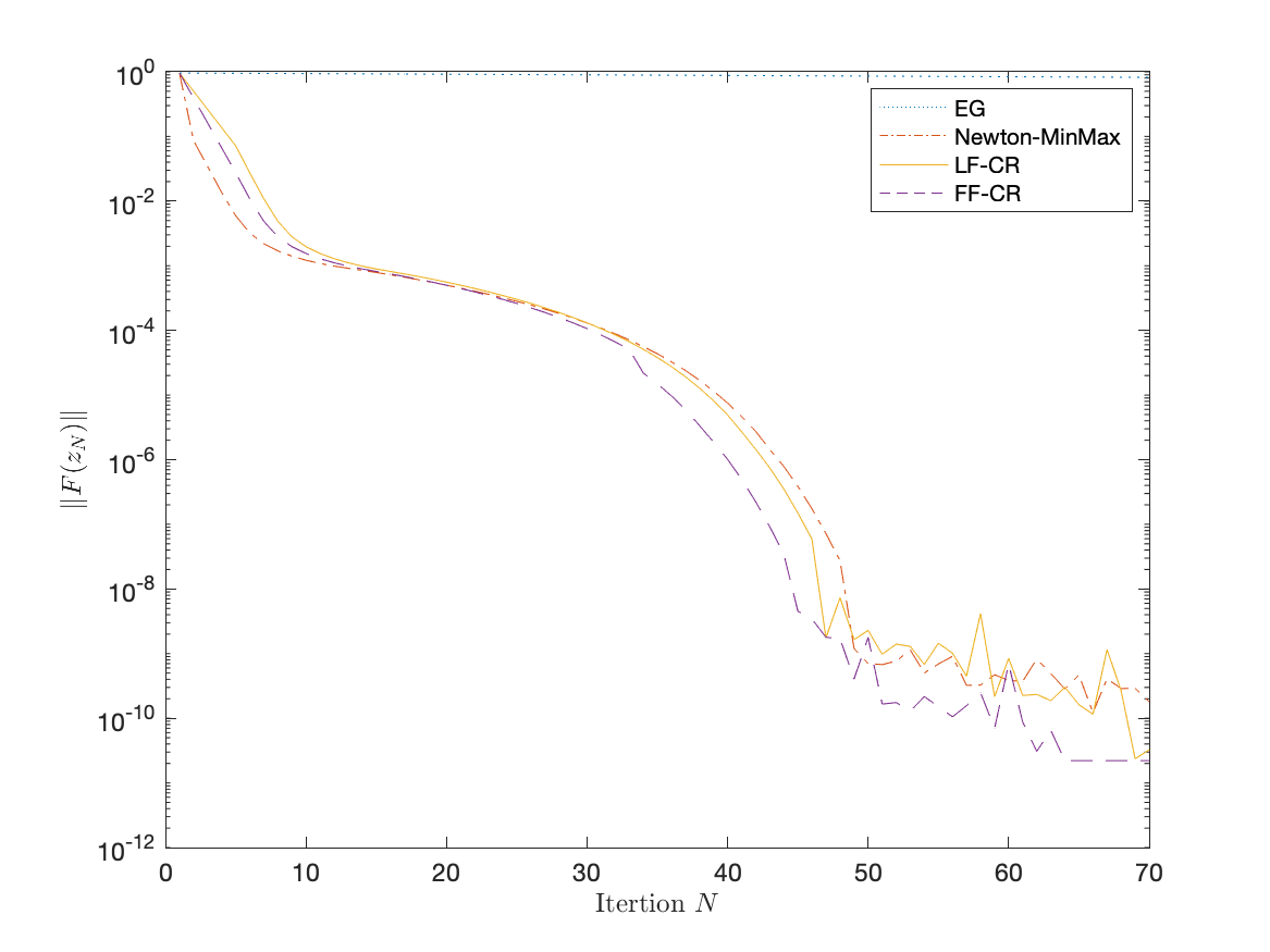
(a) n=50, $\rho$=10

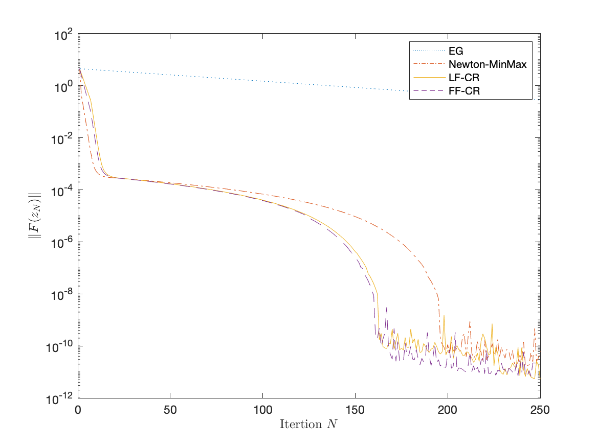
(b) n=50, $\rho$=50

Figure 1: Numerical results of the LF-CR algorithm, the FF-CR algorithm, the EG algorithm and the Newton-MinMax algorithm when $\rho\in\{10,50\}$.

We consider the following convex-concave minimax optimization problem [47]:

$$\min_{x\in\mathbb{R}^{n}}\max_{y\in\mathbb{R}^{n}}\ f(x,y)=\tfrac{\rho}{6}\|x\|^{3}+y^{\top}(Ax-b),$$ (62)

where $\rho>0$, the entries of $b\in\mathbb{R}^{n}$ are generated independently from $[-1,1]$ and $A\in\mathbb{R}^{n\times n}$ is a invertible matrix. It can be verified that the function $f$ is $\rho$-Hessian Lipschitz, and admits a global saddle point $z^{\star}=(x^{\star},y^{\star})$ with $x^{\star}=A^{-1}b$ and $y^{\star}=-\frac{\rho}{2}\|x^{\star}\|(A^{\top})^{-1}x^{\star}$.

Experimental setup. In our experiment, the problem parameters are chosen as $n=50,\rho\in\{10,50\},A=I_{n}.$ Let $H_{0}$ be the initial estimate of Hessian Lipschize constant $\rho$ and $D_{0}$ be the initial estimate of $\|z_{0}-z^{*}\|$. The initial point of all algorithms is chosen as $z_{0}=z^{*}+0.1c$, where each component of $c\in\mathbb{R}^{2n\times 1}$ is random generated independently from $[-1,1]$.

For the EG algorithm, the stepsize is set to $0.01$ and $0.001$ when $\rho=10$ and $50$, respectively. For the LF-CR algorithm and the FF-CR algorithm, we set $H_{0}=1$, $D_{0}$=$1$. For fair comparison, we use the same solver to solve the subproblems of different algorithms. We use the gradient norm as the performance indicator of the algorithm.

Results. Figure 1 shows the gradient norm descent curves of the four algorithms. Obviously, the second-order methods perform better than the first-order method, i.e., the EG method. Among the three second-order methods, the LF-CR algorithm and the FF-CR algorithm perform better than the Newton-MinMax algorithm, especially when the Lipschtiz constant, $\rho$, increases. The reason is that the Newton-MinMax algorithm uses an accurate global Hessian Lipschitz constant, which makes the step size selection of the algorithm more conservative, while the LF-CR algorithm only estimates the Hessian Lipschitz constant locally, giving more freedom to the step size selection. Although the FF-CR algorithm is completely parameter-free, its performance is similar to that of the LF-CR algorithm, which shows its efficiency.

5 Conclusions

In this paper, we propose parameter-free second-order algorithms for unconstrained convex-concave minimax optimization problems with optimal iteration complexity. Under a mild assumption that the Hessian is Lipschitz continuous, the proposed LF-CR algorithm achieves an iteration complexity of $\mathcal{O}(\frac{\rho\|z^{0}-z^{*}\|^{3}}{\epsilon})^{\frac{2}{3}}$ in terms of the $\epsilon$-optimal solution of the restricted primal-dual gap without prior knowledge of the Lipschitz constants, and the proposed FF-CR algorithm achieves an iteration complexity of $\mathcal{O}(\frac{\rho\|z^{0}-z^{*}\|^{2}}{\epsilon})^{\frac{2}{3}}$ in terms of the $\epsilon$-optimal solution of the gradient norm without any prior knowledge of problem parameters. To the best of our knowledge, the FF-CR algorithm is the first fully parameter-free second-order method for solving minimax optimization problems.

The only disadvantage of the proposed FF-CR algorithm is that it requires the exact optimal solutions of the subproblems. If the subproblem is allowed to be solved inexactly, whether the fully parameter-free algorithm with the optimal iteration complexity can still be obtained is worth further study.

References

• [1] A. Ben-Tal, L. EL Ghaoui, and A. Nemirovski. Robust Optimization, volume 28. Princeton University Press, 2009.
• [2] A. Beznosikov, A. Sadiev, and A. Gasnikov. Gradient-free methods with inexact oracle for convex-concave stochastic saddle-point problem. International Conference on Mathematical Optimization Theory and Operations Research. Springer, Cham, 105–119, 2020.
• [3] A. Mokhtari, A. Ozdaglar, and S. Pattathil. A unified analysis of extra-gradient and optimistic gradient methods for saddle point problems: proximal point approach. International Conference on Artificial Intelligence and Statistic, pages 1497–1507, PMLR, 2020.
• [4] A. Mokhtari, A. E. Ozdaglar, and S. Pattathil. Convergence rate of $\mathcal{O}(1/k)$ for optimistic gradient and extragradient methods in smooth convex-concave saddle point problems. SIAM Journal on Optimization, 30(4):3230–3251, 2020.
• [5] A. Nemirovski. Prox-method with rate of convergence $\mathcal{O}(1/t)$ for variational inequalities with Lipschitz continuous monotone operators and smooth convex-concave saddle point problems. SIAM Journal on Optimization, 15(1):229–251, 2004.
• [6] A. Sadiev, A. Beznosikov, P. Dvurechensky, and A. Gasnikov. Zeroth-order algorithms for smooth saddle-point problems. International Conference on Mathematical Optimization Theory and Operations Research. Springer, Cham, 71–85, 2021.
• [7] A. Sinha, H. Namkoong, and J. Duchi. Certifiable distributional robustness with principled adversarial training. International Conference on Learning Representations, 2018.
• [8] B. Bullins and K. A. Lai. Higher-order methods for convex-concave min-max optimization and monotone variational inequalities. SIAM Journal on Optimization, 32(3):2208–2229, 2022.
• [9] C. Jin, P. Netrapalli, and M. I. Jordan. Minmax optimization: stable limit points of gradient descent ascent are locally optimal. International conference on machine learning, PMLR, 4880–4889, 2020.
• [10] C. Liu and L. Luo. Regularized Newton methods for monotone variational inequalities with H$\ddot{o}$lder continuous Jacobians. arXiv preprint arXiv:2212.07824, 2022.
• [11] D. A. Blackwell and M. A. Girshick. Theory of Games and Statistical Decisions. Courier Corporation, 1979.
• [12] D. Adil, B. Bullins, A. Jambulapati, and S. Sachdeva. Line search-free methods for higher-order smooth monotone variational inequalities. arXiv preprint arXiv:2205.06167, 2022.
• [13] D. M. Ostrovskii, A. Lowy, and M. Razaviyayn. Efficient search of first-order nash equilibria in nonconvex-concave smooth min-max problems. SIAM Journal on Optimization, 31(4):2508–2538, 2021.
• [14] F. Huang, S. Gao, J. Pei, and H. Huang. Accelerated zeroth-order and first-order momentum methods from mini to minimax optimization. Journal of Machine Learning Research, 23:1–70, 2022.
• [15] F. Stonyakin, A. Gasnikov, P. Dvurechensky, M. Alkousa, and A. Titov. Generalized mirror prox for monotone variational inequalities: universality and inexact oracle. Journal of Optimization Theory and Applications, 194(3):988–1013,2022.
• [16] G. Lan, Y. Ouyang, and Z. Zhang. Optimal and parameter-free gradient minimization methods for convex and nonconvex optimization. arXiv preprint arXiv:2310.12139, 2023.
• [17] G. Kotsalis, G. Lan, and T. Li. Simple and optimal methods for stochastic variational inequalities, I: Operator extrapolation. SIAM Journal on Optimization, 32(3):2041–2073, 2022.
• [18] G. M. Korpelevich. The extragradient method for finding saddle points and other problems. Matecon, 12:747–756, 1976.
• [19] H. Rafique, M. Liu, Q. Lin, and T. Yang. Weakly-convex?concave min?max optimization: provable algorithms and applications in machine learning. Optimization Methods and Software, 37(3):1087–1121, 2022.
• [20] I. Goodfellow, J. Pouget-Abadie, M. Mirza, B. Xu, D. Warde-Farley, S. Ozair, A. Courville, and Y. Bengio. Generative adversarial nets. Advances in Neural Information Processing Systems, pages 2672–2680, 2014.
• [21] J. A. Hanley and B. J. McNeil. The meaning and use of the area under a receiver operating characteristic (ROC) curve. Radiology, 143(1):29–36, 1982.
• [22] J. Shen, Z. Wang, and Z. Xu. Zeroth-order single-loop algorithms for nonconvex-linear minimax problems. Journal of Global Optimization, 87:551–580, 2023.
• [23] J. Von Neumann and O. Morgenstern. Theory of Games and Economic Behavior. Princeton University Press, 1953.
• [24] J. Zhang, P. Xiao, R. Sun, and Z. Luo. A single-loop smoothed gradient descent-ascent algorithm for nonconvex-concave min-max problems. Advances in Neural Information Processing Systems, 33:7377–7389, 2023.
• [25] K. Huang, J. Zhang, and S. Zhang. Cubic regularized Newton method for the saddle point models: A global and local convergence analysis. Journal of Scientific Computing, 91(2):1–31, 2022.
• [26] K. Huang and S. Zhang. An approximation-based regularized extra-gradient method for monotone variational inequalities. arXiv preprint arXiv: 2210.04440, 2022.
• [27] K. K. Thekumparampil, P. Jain, P. Netrapalli, and S. Oh. Efficient algorithms for smooth minimax optimization. Advances in Neural Information Processing Systems, 12680–12691, 2019
• [28] L. D. Popov. A modification of the Arrow-Hurwicz method for search of saddle points. Mathematical notes of the Academy of Sciences of the USSR, 28(5):845–848, 1980.
• [29] L. Luo, Y. Li, and C. Chen. Finding second-order stationary points in nonconvex-strongly-concave minimax optimization. Advances in Neural Information Processing Systems, pages 36667–36679, 2022.
• [30] M. Arjovsky, S. Chintala, and L. Bottou. Wasserstein generative adversarial networks. International Conference on Machine Learning, PMLR, pages 214–223, 2017.
• [31] M. Nouiehed, M. Sanjabi, T. Huang, and J. D. Lee. Solving a class of non-convex min-max games using iterative first order methods. Advances in Neural Information Processing Systems, 14934–14942, 2019.
• [32] M. V. Solodov and B. F. Svaiter. A hybrid approximate extragradient-proximal point algorithm using the enlargement of a maximal monotone operator. Set-Valued Analysis, 7(4):323–345, 1999.
• [33] P. Dvurechensky, A. Gasnikov, P. Ostroukhov, C.A. Uribe, and A. Ivanova. Near-optimal tensor methods for minimizing the gradient norm of convex functions and accelerated primal?dual tensor methods. Optimization Methods and Software, 1–36, 2024.
• [34] P. Ostroukhov, R. Kamalov, P. Dvurechensky, and A. Gasnikov. Tensor methods for strongly convex strongly concave saddle point problems and strongly monotone variational inequalities. arXiv preprint arXiv:2012.15595, 2020.
• [35] P. Tseng. On linear convergence of iterative methods for the variational inequality problem. Journal of Computational and Applied Mathematics, 60(1-2):237–252, 1995.
• [36] R. D. C. Monteiro and B. F. Svaiter. Iteration-complexity of a Newton proximal extragradient method for monotone variational inequalities and inclusion problems. SIAM Journal on Optimization, 22(3):914–935, 2012.
• [37] R. I. Bot and A. Böhm. Alternating proximal-gradient steps for (stochastic) nonconvex-concave minimax problems. SIAM Journal on Optimization, 33(3):1884–1913, 2023.
• [38] R. Gao and A.J. Kleywegt. Distributionally robust stochastic optimization with wasserstein distance. Mathematics of Operations Research, 48(2):603–655, 2023.
• [39] R. Jiang and A. Mokhtari. Generalized optimistic methods for convex-concave saddle point problems. arXiv preprint arXiv: 2202.09674, 2022.
• [40] R. Jiang, A. Kavis, Q. Jin, S. Sanghavi, and A. Mokhtari. Adaptive and optimal second-order optimistic methods for minimax optimization. arXiv preprint arXiv:2406.02016, 2024.
• [41] S. Liu, S. Lu, X. Chen, Y. Feng, K. Xu, A. Al-Dujaili, and U. M. O’Reilly. Min-max optimization without gradients: convergence and applications to black-box evasion and poisoning attacks. International conference on machine learning. PMLR, 6282–6293, 2020.
• [42] S. Lu, I. Tsaknakis, M. Hong, and Y. Chen. Hybrid block successive approximation for one-sided nonconvex min-max problems: algorithms and applications. IEEE Transactions on Signal Processing, 68:3676–3691, 2020.
• [43] S. Zhang, J. Yang, C. Guzmán, N. Kiyavash, and N. He. The complexity of nonconvex-strongly-concave minimax optimization. Uncertainty in Artificial Intelligence, PMLR, 482–492, 2021.
• [44] T. Lin, C. Jin, amd M. I. Jordan. On gradient descent ascent for nonconvex-concave minimax problems. International Conference on Machine Learning, PMLR, 6083–6093, 2020.
• [45] T. Lin, C. Jin, amd M. Jordan. Near-optimal algorithms for minimax optimization. Conference on Learning Theory, PMLR, 2738–2779, 2020.
• [46] T. Lin and M. I. Jordan. Perseus: a simple high-order regularization method for variational inequalities. Mathematical Programming, 1–42, 2024.
• [47] T. Lin , P. Mertikopoulos and M. I. Jordan. Explicit second-order min-max optimization methods with optimal convergence guarantee. arXiv preprint arXiv:2210.12860, 2022.
• [48] T. Xu, Z. Wang, Y. Liang, and H. V. Poor. Gradient free minimax optimization: Variance reduction and faster convergence. arXiv preprint arXiv:2006.09361, 2020.
• [49] T. Yao and Z. Xu. Two trust region type algorithms for solving nonconvex-strongly concave minimax problems. arXiv preprint arXiv:2402.09807, 2024.
• [50] W. Kong and R. D. C. Monteiro An accelerated inexact proximal point method for solving nonconvex concave min-max problems. SIAM Journal on Optimization, 31(4):2558–2585, 2021.
• [51] W. Pan, J. Shen, Z. Xu. An efficient algorithm for nonconvex-linear minimax optimization problem and its application in solving weighted maximin dispersion problem. Computational Optimization and Applications, 78(1):287–306, 2021.
• [52] Y. Nesterov and B. T. Polyak. Cubic regularization of Newton method and its global performance. Mathematical Programming, 108(1):177–205, 2006.
• [53] Y. Nesterov. Cubic Regularization of Newton’s Method for Convex Problems with Constraints. CORE Discussion Paper, 2006.
• [54] Y. Nesterov. Dual extrapolation and its applications to solving variational inequalities and related problems. Mathematical Programming, 109(2):319–344, 2007.
• [55] Y. Nesterov. Universal gradient methods for convex optimization problems. Mathematical Programming, 152:381–404, 2015.
• [56] Y. Nesterov. Lectures on Convex Optimization. Springer, 2018.
• [57] Y-G. Hsieh, F. Iutzeler, J. Malick, and P. Mertikopoulos. On the convergence of single-call stochastic extra-gradient methods. Advances in Neural Information Processing Systems, pages 6938–6948, 2019.
• [58] Y. Ouyang and Y. Xu. Lower complexity bounds of first-order methods for convex-concave bilinear saddle-point problems. Mathematical Programming, 185(1):1–35, 2021.
• [59] Y. Ying, L. Wen, and S. Lyu. Stochastic online AUC maximization. Advances in Neural Information Processing Systems, pages 451–459, 2016.
• [60] Z. Chen, Z. Hu, Q. Li, Z. Wang and Y. Zhou. A cubic regularization approach for finding local minimax points in nonconvex minimax optimization. Transactions on Machine Learning Research, 2835–8856, 2023.
• [61] Z. Wang, K. Balasubramanian, S. Ma, and M. Razaviyayn. Zeroth-order algorithms for nonconvex minimax problems with improved complexities. arXiv preprint arXiv:2001.07819, 2020.
• [62] Z. Xu, Z. Wang, J. Wang, and Y. Dai. Zeroth-order alternating gradient descent ascent algorithms for a class of nonconvex-nonconcave minimax problems. Journal of Machine Learning Research, 24(313):1–25, 2023.
• [63] Z. Xu, Z. Wang, J. Shen, and Y. Dai. Derivative-free alternating projection algorithms for general nonconvex-concave minimax problems. SIAM Journal on Optimization, 34(2): 1879–1908, 2024.
• [64] Z. Xu, H. Zhang, Y. Xu, and G. Lan. A unified single-loop alternating gradient projection algorithm for nonconvex-concave and convex-nonconcave minimax problems. Mathematical Programming, Series A, 201:635–706, 2023.