Safety-Critical Control with Uncertainty Quantification using
Adaptive Conformal Prediction

Abstract

Safety assurance is critical in the planning and control of robotic systems. For robots operating in the real world, the safety-critical design often needs to explicitly address uncertainties and the pre-computed guarantees often rely on the assumption of the particular distribution of the uncertainty. However, it is difficult to characterize the actual uncertainty distribution beforehand and thus the established safety guarantee may be violated due to possible distribution mismatch. In this paper, we propose a novel safe control framework that provides a high-probability safety guarantee for stochastic dynamical systems following unknown distributions of motion noise. Specifically, this framework adopts adaptive conformal prediction to dynamically quantify the prediction uncertainty from online observations and combines that with the probabilistic extension of the control barrier functions (CBFs) to characterize the uncertainty-aware control constraints. By integrating the constraints in the model predictive control scheme, it allows robots to adaptively capture the true prediction uncertainty online in a distribution-free setting and enjoys formally provable high-probability safety assurance. Simulation results on multi-robot systems with stochastic single-integrator dynamics and unicycle dynamics are provided to demonstrate the effectiveness of our framework.

I Introduction

Safety-critical control plays a key role in many robotic applications, such as multi-robot navigation [1, 2] and autonomous driving [3]. Model-based approaches such as the control barrier functions (CBFs) [4, 5] have been widely applied to enforce formally provable safety for deterministic dynamical systems. However, realistic factors such as uncertainty, non-determinism, and lack of complete information often make it challenging to provide safety assurance for those stochastic dynamical systems in the real world.

Existing works on uncertainty-aware safety-critical control primarily focus on incorporating assumptions regarding specific uncertainty distributions or adopting conservative bounds. Examples include the Gaussian representation [6, 7], the bounded uniform distribution [8], and conservative bounding volumes [9]. Such approaches enable the explicit modeling of uncertainty’s impact on ensuring safety which can thus be used for safe control designs. For instance, model predictive path integral (MPPI) [10, 11] as a model-based method has been employed in various applications to account for constrained optimal control for stochastic dynamical systems. It generates sampling trajectories parallelly based on the assumed Gaussian distribution of the control policy and then derives the near-optimal control policy. To address unmodeled uncertainties, safe learning techniques have been proposed [12, 13] to heuristically quantify the uncertainty during exploration and combine it with control theoretic approaches for safe operations. However, the safety guarantee derived in these works heavily relies on the accuracy of the assumed or learned uncertainty distribution, and it remains challenging for robots operating in more realistic scenarios where the uncertainty distributions could be arbitrary and difficult to learn.

Recently, statistical techniques such as conformal prediction (CP) [14, 15] have been prevalent given their ability to quantify the prediction uncertainty of the employed machine learning or dynamics models. CP leverages a sequence of calibration data to create prediction sets that are likely to cover the true value with high probability. However, the assumption of static data distribution does not apply to many robotic applications where robots could often operate in uncertain and dynamic environments. To address this limitation, the concept of Adaptive Conformal Prediction (ACP) has been introduced in [16, 17] that can adaptively adjust the uncertainty quantification to maintain prediction accuracy under distribution shift. This enables the system to address safety-critical control when the underlying uncertainty distribution of the environment is not static but evolves over time. For example, work in [18] adopts the distance-based condition between the robot and the obstacles as constraints quantified by the ACP and embeds them to the model predictive control (MPC) framework to produce the collision-free path. However, as suggested in [19] the distance-based safety constraint in the MPC framework may require a longer horizon for effective collision avoidance and thus unnecessarily increase the computational time.

In this paper, we propose a novel uncertainty-aware safe control framework that integrates the probabilistic CBFs with adaptive conformal prediction for stochastic dynamical system with unknown motion noise. The framework is able to provably quantify the uncertainty of future robot states predicted by the stochastic system dynamics model, and utilize them to design CBF-based control constraints for high-probabilty safety guarantee. The contributions in this paper are threefold:

• We propose a novel provable probabilistic safe barrier certificate with Adaptive Conformal Prediction (ACP-SBC) for safe control under unknown motion noise.

• Theoretical analysis are provided to justify the enforced high-probability safety guarantee of our proposed method, where the derived guarantee under quantified uncertainty is distribution-free, i.e. it does not require knowing the distribution of motion noise as a prior.

• Simulation results on multi-robot systems are provided to evaluate the effectiveness of the proposed framework.

II Preliminaries and Problem formulation

II-A Control Barrier Functions

Consider the robot dynamics as the following control affine system,

$$\dot{x}=f(x)+g(x)u$$ (1)

where $x\in\mathbb{R}^{n}$ is the robot state and $u\in\mathbb{R}^{m}$ is the control input. $f:\mathbb{R}^{n}\mapsto\mathbb{R}^{n}$ and $g:\mathbb{R}^{n}\mapsto{\mathbb{R}^{n\times m}}$ are locally Lipschitz continuous.

Control barrier functions (CBFs) [4] are often designed to ensure the robot’s safety. The set of robot states satisfying the safety constraints can be denoted by $\mathcal{H}$ and expressed as the zero-superlevel set of a continuously differentiable function $h(x):\mathbb{R}^{n}\mapsto\mathbb{R}$,

$$\mathcal{H} =\left\{x\in\mathbb{R}^{n}|h(x)\geqslant 0\right\},$$

$$\partial\mathcal{H} =\left\{x\in\mathbb{R}^{n}|h(x)=0\right\},$$ (2)

$$\mathrm{Int}(\mathcal{H}) =\left\{x\in\mathbb{R}^{n}|h(x)>0\right\}.$$

where $\partial\mathcal{H}$ and $\mathrm{Int}(\mathcal{H})$ define the boundary and interior of the safe set $\mathcal{H}$, respectively.

Lemma 1

CBFs. [Summarized from [4]] Given the system dynamics Eq.(1) affine in control and the safe set $\mathcal{H}$ as the 0-super level set of a continuously differentiable function $h(x):\mathbb{R}^{n}\mapsto\mathbb{R}$, the function $h$ is called a control barrier function if there exists an extended class-$\mathcal{K}$ function $\mathcal{K}(\cdot)$, such that $\sup_{u\in\mathbb{R}^{m}}\{\dot{h}(x,u)\}\geq-\mathcal{K}(h(x))$ for all $x\in\mathbb{R}^{n}$. The admissible control space for any Lipschitz continuous controller $u\in\mathbb{R}^{m}$ rendering $\mathcal{H}$ forward invariant (i.e., keeping the system state $x$ staying in $\mathcal{H}$ overtime) thus becomes:

$$\mathcal{B}(x)=\left\{u\in\mathcal{U}|L_{f}h(x)+L_{g}h(x)u+\mathcal{K}(h(x))\geqslant 0\right\}$$ (3)

where $L_{f}h$ and $L_{g}h$ are the Lie derivatives of $h$ along the function $f$ and $g$ respectively. The extended class $\mathcal{K}$ function can be commonly chosen as $\mathcal{K}(h(x))=\gamma h(x)$ with $\gamma>0$ as in [8]. The condition of $B(x,u)=L_{f}h(x)+L_{g}h(x)u+\mathcal{K}(h(x))\geqslant 0$ in Eq.(3) can be used to denote the safety barrier certificates (SBC) [1] that define satisfying controller $u$ for the robot to stay within the safe set $\mathcal{H}$.

II-B Chance-Constrained Safety

Even though the Lemma 1 reveals the explicit condition for robot safety with the perfect observation of the robot motion, the presence of the uncertainty makes it challenging to enforce the safe set $\mathcal{H}$ forward invariant, or even impossible when the motion noise is unknown. In this paper, we consider the realistic situation where the robot system dynamics is stochastic and has the unknown random motion noise. With that, we consider the discrete-time stochastic control-affine system dynamics as follows,

$$\hat{x}_{k+1}=\tilde{f}(\hat{x}_{k})+\tilde{g}(\hat{x}_{k})u_{k}+\epsilon_{k}$$ (4)

where $\hat{x}_{k}\in\mathbb{R}^{n}$ is the robot state and $u_{k}\in\mathbb{R}^{m}$ is the control input. $\tilde{f}:\mathbb{R}^{n}\mapsto\mathbb{R}^{n}$ and $\tilde{g}:\mathbb{R}^{n}\mapsto{\mathbb{R}^{n\times m}}$ are locally Lipschitz continuous. $\epsilon_{k}$ is the unknown random motion noise. Note the distribution of the noise $\epsilon_{k}$ is unknown and may evolve over time, which makes the safety-critical control problem more challenging. To satisfy the safety constraint defined by Eq.(2), we consider this problem in a chance-constrained setting. Formally, given the user-defined failure probability $\beta\in(0,1)$ for the safety condition, we have:

$$P(h(\hat{x}_{k+1})\geqslant 0)\geqslant 1-\beta.$$ (5)

where $P(\centerdot)$ is the probability under the event $(\centerdot)$.

Given the stochastic system dynamics in Eq.(4) and motivated by Probabilistic Safety Barrier Certificates in [8], the probabilistic safety constraint in Eq. (5) can be satisfied by the chance constraints over control $u_{k}$ summarized as the following lemma 2

Lemma 2

[Summarized from [8]] Given the stochastic robot system defined in Eq. (4), the robot state $\hat{x}_{k}$ is considered as a random variable at the time step $k$, and the ${\mathcal{B}}(\hat{x}_{k})$ is the corresponding admissible safe control space which renders the robot’s state $\hat{x}_{k+1}$ collision-free at time step $k+1$ if without noise. Then the probabilistic constraint on control is the sufficient condition of the probabilistic safety constraint defined in Eq. (5), which is formulated as,

$$P(u_{k}\in{\mathcal{B}}(\hat{x}_{k}))\geqslant 1-\beta\Rightarrow P(\hat{x}_{k+1}\in\mathcal{H})\geqslant 1-\beta$$ (6)

Proof:

Assuming the robot is at the safe state initially and given the definition of the safe control space in Eq.(3), we have $u_{k}\in{\mathcal{B}}(\hat{x}_{k})$ $\Rightarrow$ $\hat{x}_{k+1}\in\mathcal{H}$ and $u_{k}\notin{\mathcal{B}}(\hat{x}_{k})$ $\not\Rightarrow$ $\hat{x}_{k+1}\notin\mathcal{H}$. Therefore, we have $P(u_{k}\in{\mathcal{B}}(\hat{x}_{k}))\leqslant P(\hat{x}_{k+1}\in\mathcal{H})$ and thus Lemma 2 holds true. ∎

The work in [8] derived the deterministic admissible control space where Eq. (6) holds through assuming $\epsilon_{k}$ in Eq.(4) follows a uniform distribution known as prior. However, it is non-trivial to derive such control space when the distribution of $\epsilon_{k}$ is unknown and may be time-varying.

II-C Adaptive Conformal Prediction

Conformal Prediction (CP) [15] is a statistical method to formulate a certified region for complex prediction models without making assumptions about the prediction model.

Given a dataset $\mathcal{D}=\{(X_{k},Y_{k})\}$ (where $k=1,\dots,d$, $X_{k}\in\mathbb{R}^{n}$, and $Y_{k}\in\mathbb{R}$) and any prediction model $F:X\mapsto Y$ trained from $\mathcal{D}$, e.g. linear model or deep learning model, the goal of CP is to obtain $\bar{S}\in\mathbb{R}$ to construct a region $R(X^{*})=[F(X^{*})-\bar{S},F(X^{*})+\bar{S}]$ so that $P(Y^{*}\in R(X^{*}))\geqslant 1-\alpha$, where $\alpha\in(0,1)$ is the failure probability and $X^{*},Y^{*}$ are the testing model input and the true value respectively. We can then define the nonconformity score $S_{k}\in\mathbb{R}^{+}$ as $S_{k}=|Y_{k}-F(X_{k})|$. The large nonconformity score suggests a bad prediction of $F(X_{k})$.

To obtain $\bar{S}$, the nonconformity scores $S_{1},\dots,S_{d}$ are assumed as independently and identically distributed (i.i.d.) real-valued random variables, which allows permutating element of the set $\mathcal{S}=\{S_{1},\dots,S_{d}\}$ (assumption of exchangeability) [15]. Then, the set $\mathcal{S}$ is sorted in a non-decreasing manner expressed as $\mathcal{S}=\{S^{(1)},\dots,S^{(r)},\dots,S^{(d)}\}$ where $S^{(r)}$ is the $(1-\alpha)$ sample quantile of $\mathcal{S}$. $r$ in $S^{(r)}$ is defined as $r:=\lceil(d+1)(1-\alpha)\rceil$ where $\lceil\cdot\rceil$ is the ceiling function. Let $\bar{S}=S^{(r)}$, then the following probability holds [15],

$$P(F(X^{*})-S^{(r)}\leqslant Y^{*}\leqslant F(X^{*})+S^{(r)})\geqslant 1-\alpha$$ (7)

Thus, we can utilize $S^{(r)}$ to certify the uncertainty region over the predicted value of $Y^{*}$ given the prediction model $F$. It is noted that $P(F(X^{*})-S^{(r)}\leqslant Y^{*}\leqslant F(X^{*})+S^{(r)})\in[1-\alpha,1-\alpha+\frac{1}{1+d})$ [15] and thus the probability in the Eq.(7) holds.

Adaptive Conformal Prediction (ACP). CP relies on the assumption of exchangeability [15] about the elements in the set $\mathcal{S}$. However, this assumption may be violated easily in dynamical time series prediction tasks [16]. To achieve reliable dynamical time series prediction in a long-time horizon, the notion of ACP[17] was proposed to re-estimate the quantile number online. The estimating process is shown below:

$$\alpha_{k+1}=\alpha_{k}+\delta(\alpha-e_{k})\;\mathrm{with}\;e_{k}=\begin{aligned} \begin{cases}0,\mathrm{if}\;S_{k}\leqslant S_{k}^{(r)},\\ 1,\text{otherwise}.\end{cases}\end{aligned}$$ (8)

where $\delta$ is the user-specified learning rate. $S_{k}\in\mathbb{R}^{+}$ is the nonconformity score at time step k, and $S_{k}^{(r)}$ is the sample quantile. It is noted that if $S_{k}\leqslant S_{k}^{(r)}$, then $\alpha_{k+1}$ will increase to undercover the region induced by the quantile number $S_{k}^{(r)}$.

II-D Problem Statement

In this paper, we aim to 1) effectively quantify the chance constraints of the safe conditions and 2) integrate the probabilistic control constraint into the MPC framework for deriving satisfying control inputs. The optimization problem can be formulated as follows,

$$\min_{{u}_{k:k+H-1|k}}\,\,l_{T}(\hat{x}_{k+H|k})+\sum^{H-1}_{\tau=0}l_{s}(\hat{x}_{k+\tau|k},{u}_{k+\tau|k})$$ (9)

$$s.t. \quad\hat{x}_{k+\tau+1|k}=\tilde{f}(\hat{x}_{k+\tau|k})+\tilde{g}(\hat{x}_{k+\tau|k}){u}_{k+\tau|k}+\epsilon_{k+\tau|k},$$ (9a)

$$\quad P(u_{k+\tau|k}\in\mathcal{B})\geqslant 1-\alpha,$$ (9b)

$$\quad{u}_{k+\tau|k}\in[u_{min},u_{max}],\quad\forall\tau=0,\ldots,H-1$$ (9c)

where $\hat{x}_{k+\tau|k}$ represents the state vector at time step $k+\tau$ predicted at the time step $k$ from the current state $\hat{x}_{k}$, by applying the control input sequence ${u}_{k:k+H-1|k}$ to the system dynamics Eq.(9a). $\epsilon_{k+\tau|k}$ is the motion noise at time step $k+\tau$ estimated at the time step $k$. $H$ is the time horizon and $l_{T}(\hat{x}_{k+H|k}),l_{s}(\hat{x}_{k+\tau|k},{u}_{k+\tau|k})$ are the terminal cost and stage cost respectively. $P(u_{k+\tau|k}\in\mathcal{B})\geqslant 1-\alpha$ represents the probabilistic control constraint in this paper, and $u_{min},u_{max}$ represent the control bounds.

It is noted that the control constraints in Eq.(9b) are difficult to address due to the unknown distribution-free motion noise $\epsilon_{k}$ in the actual stochastic dynamical system in Eq. 4. We will propose a method to obtain the deterministic control constraints satisfying the chance constraints Eq.(9b) in the Section III.

III Method and algorithms

III-A Conformal Prediction for Safety Barrier Certificates

Inspired by the safety barrier certificates (SBC) in [1] with Lemma 1, we define the following terms.

$$B_{k}(x_{k},u_{k})=L_{f}h(x_{k})+L_{g}h(x_{k})u_{k}+\mathcal{K}(h(x_{k}))$$ (10)

$$\hat{B}_{k}(\hat{x}_{k},u_{k})=L_{f}h(\hat{x}_{k})+L_{g}h(\hat{x}_{k})u_{k}+\mathcal{K}(h(\hat{x}_{k}))$$ (11)

Remark 1

$B_{k}(x_{k},u_{k})$ is considered as a prediction function similar to the function $F(X)$ in section II-C, which is a reasonable assumption proved in Proposition 1. Note that although the continuous-time CBF is adopted here with $L_{f}h,L_{g}h$ to compute $B_{k},\hat{B}_{k}$, they can be transformed into the discrete forms as done in [20, 12].

Given the Eq.(10) and Eq.(11), the nonconformity score between $\hat{B}_{k}$ and $B_{k}$ at global time step $k$ is formulated as $E_{B_{k}}=|\hat{B}_{k}-B_{k}|\in\mathbb{R}^{+}$. $E_{B_{k}}$ will be stored in a non-decreasing order to construct the non-conformity score set $\mathfrak{E}$. The $1-\alpha$ sample quantile of the set $\mathfrak{E}$ is expressed as $E_{B_{k}}^{(r)}$ with $r=\lceil k(1-\alpha)\rceil$ where $\lceil\cdot\rceil$ is the ceiling function. Then, the following holds given Eq.(7),

$$P(|\hat{B}_{k}-B_{k}|\leqslant E_{B_{k}}^{(r)})\geqslant 1-\alpha$$ (12)

Theorem 1

Given the quantile number $E^{(r)}_{B_{k}}$ from the set $\mathfrak{E}$ and the failure probability $\alpha\in(0,1)$, the state-dependent control space $\mathcal{\tilde{B}}(\hat{x}_{k})$ defined as follows can lead to the same probability guarantee of safety constraint, i.e. $P(h(\hat{x}_{k+1})\geqslant 0)\geqslant 1-\alpha$.

$$\mathcal{\tilde{B}}(\hat{x}_{k})=\left\{u_{k}\in\mathcal{U}|B_{k}-E^{(r)}_{B_{k}}\geqslant 0\right\}$$ (13)

Proof:

We have $P(|\hat{B}_{k}-B_{k}|\leqslant E_{B_{k}}^{(r)})\geqslant 1-\alpha$. Given $|\hat{B}_{k}-B_{k}|\leqslant E_{B_{k}}^{(r)}$, the following formulation holds: $-E_{B_{k}}^{(r)}\leqslant\hat{B}_{k}-B_{k}\leqslant E_{B_{k}}^{(r)}$, $B_{k}-E_{B_{k}}^{(r)}\leqslant\hat{B}_{k}\leqslant B_{k}+E_{B_{k}}^{(r)}$. Since $B_{k}\geqslant 0$ is guaranteed by the CBFs and $E_{B_{k}}^{(r)}\in\mathbb{R}^{+}$, this equation holds only by

$$B_{k}-E_{B_{k}}^{(r)}=L_{f}h(x_{k})+L_{g}h(x_{k})u_{k}+\mathcal{K}(h(x_{k}))-E_{B_{k}}^{(r)}\geqslant 0.$$ (14)

With Lemma 2, it yields $P(h(\hat{x}_{k+1})\geqslant 0)\geqslant 1-\alpha$. ∎

Solving the chance constraint embedded in MPC is a challenging task since (a) it is non-trivial to quantify the time-varying noise and (b) $\hat{B}_{k}$ at future time steps is difficult to obtain. Theorem 1 transfers the chance constraint to a deterministic constraint to make MPC solvable. We just consider the one-step ($\tau=1$) SBC for MPC horizon for analysis convenience. The multi-step SBC for MPC is analyzed in III-B.

Proposition 1

Given the robot state $\hat{x}_{k}\in\mathbb{R}^{n}$ generated by Eq.(4), let the non-conformity score of the robot state expressed by $E_{x_{k}}=||\hat{x}_{k}-x_{k}||$. Then $E_{B_{k}}=|\hat{B}_{k}-B_{k}|\leqslant\mathcal{L}||\hat{x}_{k}-x_{k}||=\mathcal{L}E_{x_{k}}$ holds where $\mathcal{L}=(\mathcal{L}_{L_{f}h}+\mathcal{L}_{L_{g}h}||u_{k}||+\mathcal{L}_{\mathcal{K}h})$ with $\mathcal{L}_{(\cdot)}$ as the Lipschitz constant under the function $(\cdot)$. This validates the existence of Eq.(12).

Proof:

With $B_{k},\hat{B}_{k}$ defined in Eq.(10) and (11), the following derivation holds:

$$|\hat{B}_{k}-B_{k}|= |L_{f}h(\hat{x}_{k})+L_{g}h(\hat{x}_{k})u_{k}+\mathcal{K}(h(\hat{x}_{k}))$$

$$-L_{f}h(x_{k})-L_{g}h(x_{k})u_{k}-\mathcal{K}(h(x_{k}))|$$

$$= |L_{f}h(\hat{x}_{k})-L_{f}h(x_{k})+L_{g}h(\hat{x}_{k})u_{k}$$

$$-L_{g}h(x_{k})u_{k}+\mathcal{K}(h(\hat{x}_{k}))-\mathcal{K}(h(x_{k}))|$$

$$\leqslant (\mathcal{L}_{L_{f}h}+\mathcal{L}_{L_{g}h}||u_{k}||+\mathcal{L}_{\mathcal{K}h})||\hat{x}_{k}-x_{k}||$$

$$= \mathcal{L}E_{x_{k}}.$$

∎

Proposition 1 not only shows the existence of Eq.(12), but also allows control constraints in Eq.(14) to be integrated into the MPC framework. Recall that the robot may move under the motion noise with time-varying distribution, which could easily break the i.i.d. assumption of the nonconformity score set. Through Proposition 1, $\mathcal{L}$ connects $E_{B_{k}}$ and $E_{x_{k}}$, and thus if the set constructed from the element $E_{x_{k}}$ is not i.i.d., then the set $\mathfrak{E}$ is not i.i.d.. Therefore, it is reasonable to adopt ACP to quantify Eq.(12).

III-B Adaptive Conformal Prediction for MPC

The safety constraint in the optimization problem (Eq.(9)) is computed by Eq.(14) in Theorem 1. However, $E_{B^{\tau}_{k}}=|\hat{B}^{\tau}_{k}-B^{\tau}_{k}|$ (where $\tau$ is the MPC horizon time step) can not be obtained because we can not acquire $\hat{B}^{\tau}_{k}$ at the future MPC horizon time step under unknown motion noise. Hence, we cannot compute the $\alpha_{k}$ in Eq.(8). We will adopt the time-lagged method from [18] to tackle this problem.

Fig. 1: Computation steps for time-lagged ACP. In the current time horizon ($H=3$) starting at time step $k$, the time-lagged error of CBFs can be computed by $E^{\tau}_{B_{k}}=|\hat{B}_{k}-B^{\tau}_{k-\tau}|$. Then, $E^{\tau}_{B_{k}}$, $\tau=1,\dots,H$, are stored in the nonconformity set $\mathfrak{E}$.

The method of ACP for MPC in [18] utilized $\tau$ step-ahead nonconformity score to represent the future nonconformity score, which is named the time-lagged method. The computation process is presented in Fig.1.

However, the time-lagged method does not provide a certain probability coverage guarantee, and the probability coverage of the safety constraint throughout the entire MPC horizon is still not assured. The theoretic analysis of these two issues were provided by [18], which is summarized as follows.

Lemma 3

ACP Probability Guarantee. Given the learning rate $\delta$, the initial failure probability $\alpha_{0}\in(0,1)$, and the MPC’s horizon $H$. Eq.(12) under MPC’s horizon is bounded by,

$1-\alpha-p_{1}\leqslant\frac{1}{H}\sum_{k=1}^{H}P(E_{B_{k}}\leqslant E_{B_{k}}^{(r)})\leqslant 1-\alpha+p_{2}$, where $p_{1}=\frac{\alpha_{0}+\delta}{H\delta}$, $p_{2}=\frac{1-\alpha_{0}+\delta}{H\delta}$ so that $\lim_{H\to\infty}p_{1}=0$ and $\lim_{H\to\infty}p_{2}=0$

Proposition 2

Probability Guarantee under MPC. The probability of the safe constraint under MPC will converge to $1-\alpha-p$,

$$\frac{1}{H}\sum_{k=1}^{H}P(h(\hat{x}_{k+1})\geqslant 0)\geqslant 1-\alpha-p$$ (15)

where $p=(\alpha+\delta)/(H\delta)$ is a constant related to the learning rate $\delta$, the MPC horizon $H$. When the MPC horizon $H\rightarrow\infty$, the algorithm will converge to $1-\alpha$. The proof can be found in [18].

III-C Algorithm Analysis

Input: Parameters: ACP failure probability $\alpha$ and learning rate $\delta$, prediction horizon $H$, $\gamma$ in CBFs, total time steps $tn$, time step $ts$, initial safe state $x_{0}$ and goal state $x_{g}$

Output: Safe path of the robot

1

Initialization: $x_{0}$; 2

while $k\leqslant tn$ do 3

foreach $\tau<H$ do 4

    $B_{k}^{\tau}\leftarrow L_{f}h(x_{k}^{\tau})+L_{g}h(x_{k}^{\tau})u_{k}^{\tau}+\gamma h(x_{k}^{\tau})$ ; 5

       $E_{B_{k}^{\tau}}\leftarrow|\hat{B}_{k}-B_{k-\tau}^{\tau}|$ ; 6

       $\mathfrak{E}\leftarrow E_{B_{k}^{\tau}}$ ; 7

       $E_{B_{k}^{\tau}}^{(r)}\leftarrow(\lceil k(1-\alpha)\rceil)^{\mathrm{th}}$ of $\mathfrak{E}$; 8

       $\hat{B}_{k}^{\tau}\leftarrow B_{k}^{\tau}-E_{B_{k}^{\tau}}^{(r)}$ ; 9

       if $E_{B_{k}^{\tau}}\leqslant E_{B_{k}^{\tau}}^{(r)}$ then 10

       $\alpha_{k+1}^{\tau}=\alpha_{k}^{\tau}+\delta\alpha$ ; 11

          else 12

       $\alpha_{k+1}^{\tau}=\alpha_{k}^{\tau}+\delta(\alpha-1)$ ; 13

          end if 14

       end foreach 15

   $u_{k}\leftarrow\mathrm{MPC}(x_{k}^{\tau},u_{k}^{\tau},\hat{B}_{k}^{\tau})\>\tau=0,\dots,H$ ; 16

    $x_{k+1}\leftarrow f(x_{k})+g(x_{k})u_{k}+\epsilon_{k}$ ; 17

    end while 18

Algorithm 1 ACP-SBC

The adaptive conformal prediction for safety barrier certificates named ACP-SBC is shown in Algorithm 1. The ACP is added to quantify the uncertainty of the chance constraint within MPC and the quantified constraint is then embedded in the optimization Eq.(9b). The existence of the chance constraint is proved in Theorem 1 and Proposition 2 illustrates the probabilistic guarantee of this framework.

III-D Case for Multi-Robot Collision Avoidance

In this subsection, we formulate a specific form of the CBFs under the safety constraint in the robot-robot case and the robot-obstacle case in order to validate ACP-SBC’s performance in the simulation experiments.

Robot-Robot Case: the safe constraint between two robots can be defined below,

$$h_{i,j}({x_{k}})=||{x}^{i}_{k}-{x}^{j}_{k}||^{2}-(R^{i}+R^{j})^{2}$$ (16)

where $R^{i},R^{j}$ represent the radius of the robots $i,j$, and ${x}^{i}_{k}$ and ${x}^{j}_{k}$ are the positions of the robot $i,j$ respectively. Then, according to Eq.(13), the corresponding constraint becomes,

$$2({x}^{i}_{k}-{x}^{j}_{k})(\triangle f^{ij}_{k}+\triangle g^{i,j}_{k}u^{ij}_{k})+\gamma h({x^{ij}_{k}})-\mathcal{L}E^{(r)}_{B_{k}}\geqslant 0$$ (17)

where $\triangle f^{ij}_{k}=f({x}^{i}_{k})-f({x}^{j}_{k})$, $\triangle g^{i,j}_{k}u^{ij}_{k})=g(x^{i}_{k})u^{i}_{k}-g(x^{j}_{k})u^{j}_{k}$.

Robot-Obstacle Case: the safe constraint between the robot and the obstacle can be defined as the following similar to the robot-robot constraints,

$$h_{i,\mathrm{o}^{j}}({x_{k}})=\left\|{x}^{i}_{k}-x^{j}_{\mathrm{o}}\right\|^{2}-(R^{i}+R^{j}_{\mathrm{o}})^{2}$$ (18)

where $x^{j}_{\mathrm{o}}$ represents the position of the obstacle $j$, which is regarded as a circle with the radius $R^{j}_{\mathrm{o}}$. Then we have,

$$2({x}^{i}_{k}-x^{j}_{\mathrm{o}})(f_{i}({x}^{i}_{k})+g(x^{i}_{k})u^{\mathrm{o}^{j},i}_{k})+\gamma h({x^{i}_{k}})-\mathcal{L}E^{(r)}_{B_{k}}\geqslant 0$$ (19)

Multi-Robot with Multi-Obstacle Case. It is noted that the control policy of the multi-robot with the obstacle can be acquired by the union set between the multi-robot safe policy and the robot-obstacle policy, which can be expressed as $u^{s}_{k}=u^{i,j}_{k}\bigcap u^{i,\mathrm{o}}_{k},\forall j\neq i$.

IV Simulation

The numerical simulations are conducted in this section to validate the effectiveness of our proposed algorithm. We first examine the impact of the specific parameters in the Algorithm 1 on the performance using a robot modeled by single integrator dynamics. Then, the simulation performance of the proposed ACP-SBC under variant noise distributions is discussed. Finally, the discussion is extended to the multi-robot collision avoidance task where behaviors of robots with both single integrator dynamics and unicycle dynamics are investigated.

IV-A Simulation Setup

To validate the performance of Algorithm 1, the stochastic dynamics of the single-integrator model is presented below:

$$\dot{x}=u+\epsilon$$ (20)

where $\epsilon$ is the motion uncertainty.

For the numerical simulations involved in the parameters analysis and performance comparison under variant noise distributions, the control input is limited by $-1\leqslant u\leqslant 1$ and the stepsize is $ts=0.05$.

To validate the performance of Algorithm 1, the time horizon $H$ of MPC, $\gamma$ in the deterministic control constraint, and the failure probability $\alpha$ in the ACP, will be analyzed to guide the following simulation. Gaussian noise $\epsilon\sim\mathcal{N}(0,1)$ is applied to the numerical simulation of the stochastic dynamics in Eq.(20) and the robot radius is $R=0$ for visualization convenience.

(a) Horizon $H$

(b) $\gamma$ in CBFs

(c) $\alpha$ in ACP

(d) $\hat{B}$ estimated by ACP-SBC

Fig. 2: The effect of the parameter in our method (ACP-SBC).

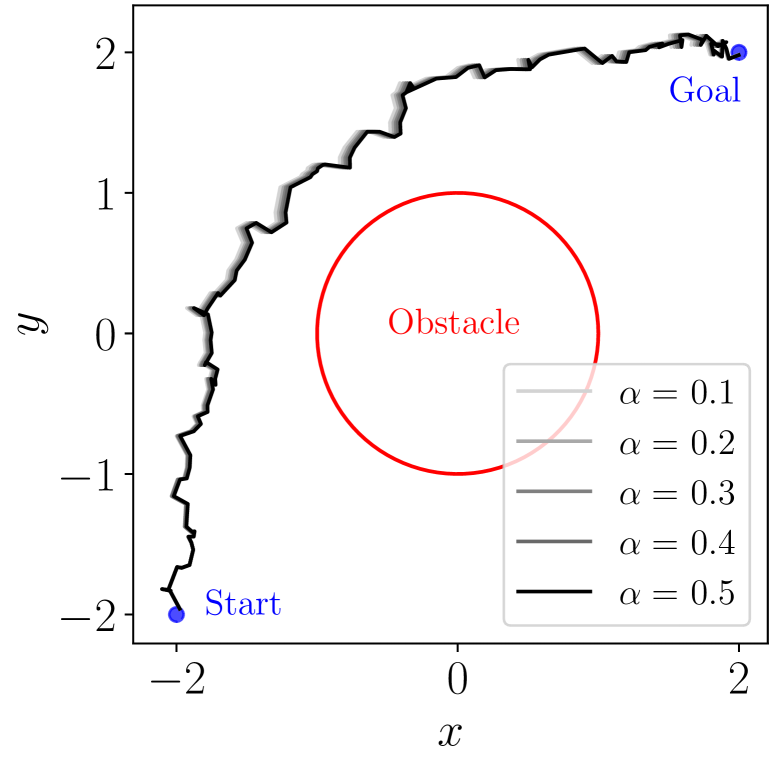
Parameter Analysis. The numerical simulation result as shown in Fig.2 for the parameter analysis illustrates that: the robot is more conservative (far away from the obstacle) when $H$ increases, $\gamma$ decreases, and $\alpha$ decreases. The result indicates that the big horizon $H$ shows more potential to avoid the obstacle because of the longer time horizon considered by the robot to get feedback from the environment. Similar to $H$, $\alpha$ decreases so the belief interval of the robot state enlarges, leading to the preservation of the robot. In the following simulation, $H=8$, $\alpha=0.05$ and $\gamma=1$ will be adopted without extra specification.

ACP Analysis. To verify the efficacy of the proposed algorithm, a comparative analysis between the ground truth and the $\hat{B}$ estimated by ACP-SBC is conducted using the same simulation environment designated for parameter analysis. The findings, illustrated in Fig.2(d), suggest that the ACP-SBC is capable of accurately estimating $\hat{B}$ with a confidence level of 95% ($\alpha=0.05$).

IV-B Distribution Comparision

(a) Noise from normal distribution

(b) Noise from unifrom distribution

(c) Noise from mixture distribution

Fig. 3: Distribution-free validation. Normal (Uniform) means that the Gaussian distribution (uniform distribution) is added to the CBFs-based method or our method (ACP-SBC) while mixture means that one of them is randomly added to the stochastic system at each time step.

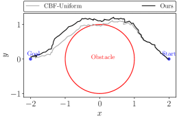
To validate the effectiveness of the proposed method, the CBFs-based method and ACP-SBC are applied to the single integrator simulation rendered by the Eq.(20). Specifically, we consider the noise following the Gaussian distribution ($\epsilon\sim\mathcal{N}(0,1)$), the uniform distribution ($\epsilon\sim U(-1,1)$), and a random combination of the two distributions. To present the numerical simulation result clearly, the robot radius $R=0$ is also applied, which can be convenient for checking the collision with the obstacle.

The simulation result in Fig.3 shows that the path generated from ACP-SBC is collision-free under different distribution inputs while all the paths collide with the obstacle using the CBFs-based method. Simulation results reveal that ACP-SBC can be applied to quantify different distributions and even the time-varying distribution.

IV-C Multi-Robot Collision Avoidance with Obstacle

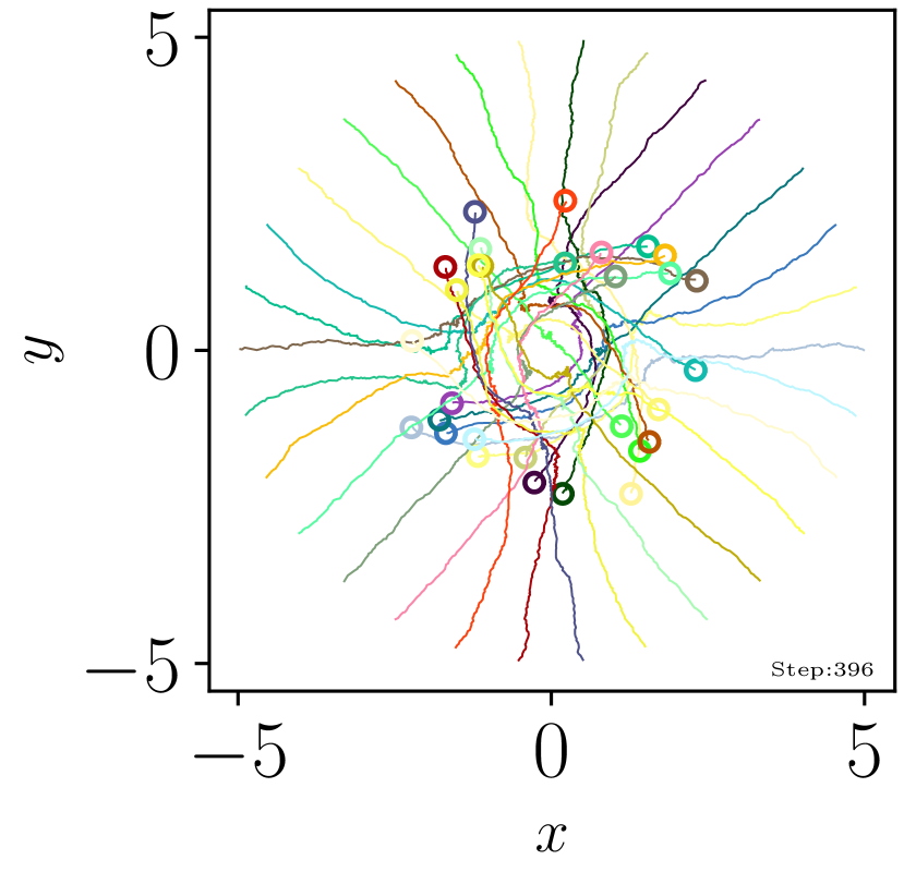
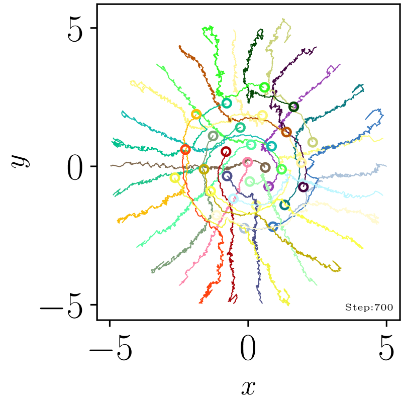
Multi-Robot Case. We continue to verify ACP-SBC in a multi-robot scenario. First, the simulation in an obstacle-free scenario with the introduction of 30 robots modeled by single integrator dynamics is conducted. All the parameters are the same as aforementioned except the robot radius ($R=0.075$).

To illustrate the results, the minimum distance is calculated at each time step, both among robots and between a robot and an obstacle. The minimum distance below the reference distance means that collision happens. The reference distance is set to 0 because it represents the difference between the distance of two robots and the safety distance.

The simulation results in Fig.4(a)-(c) present that the robot still collides using CBFs, whereas ACP-SBC guarantees that the robot avoids collisions in scenarios with up to 30 robots. The simulation involved scaling the number of robots and was repeated 20 times with 20 different random seeds. The simulation result in Fig.4(d) validates that ACP-SBC is effective when scaling up the number of robots.

Multi-Robot Collision Avoidance with Obstacle. However, all the simulations so far are based on robots with single integrator dynamics. To validate the generalization of ACP-SBC, an additional experiment based on robots with unicycle dynamics is conducted on the CoppeliaSim [21].

The robot’s radius is $R=0.075m$ and the radius of the obstacle is $R_{\mathrm{o}}=0.2m$. While the control input limit, $-0.08m/s\leqslant u\leqslant 0.08m/s$, will be adopted in the unicycle simulation. The noise $\epsilon_{v}\sim 0.01\times\mathcal{N}(0,1)$ is applied to the linear velocity of the unicycle robot, while $\epsilon_{\omega}\sim 0.001\times\mathcal{N}(0,1)$ is allpied to the angular velocity of the unicycle robot. $H=5$ is employed and step size in the simulation platform is $ts=0.05$. $\gamma=1000$ is applied because big $\gamma$ reveals the less conservative motion, which has more potential to collide. Furthermore, ACP-SBC can still work on the small $\gamma$ through the previous simulation result.

The simulation results using robots with unicycle dynamics under three obstacles are shown in Fig.5. The robot using the CBFs-based method collides under Gaussian distribution input, whereas the ACP-SBC method remains collision-free. The simulation result validates that our ACP-SBC can also be applied to the unicycle robot.

(a) CBFs

(b) Our method: ACP-SBC

(c) Minimum distance

(d) Minimum distance of robots under 20 experiments

Fig. 4: Simulation for multi-robot coordination using 30 robots with single integrator dynamics in an obstacle-free environment.

(a) CBFs

(b) Our method: ACP-SBC

(c) Minimum distance

Fig. 5: Simulation with 6 Khepera IV robots with unicycle dynamics for multi-robot coordination in CoppeliaSim with Fig.5(a) using CBFs-based method and Fig.5(b) using ACP-SBC. It is obvious that collision happens using the CBFs-based method as shown in Fig.5(a) and the minimum distance shown in Fig.5(c) also reveals that the collision, as the plot intersects the reference line, indicating that $h<0$

V Conclusion

This paper addresses the problem of uncertainty-aware safety-critical control under stochastic system dynamics with unknown motion noise. A new framework, ACP-SBC, is proposed to quantify the uncertainty without assuming specific forms of the distribution of the motion noise or the prediction model. Theoretical analysis is provided to justify the performance of our proposed method. Simulation results validate the effectiveness of the proposed ACP-SBC framework.

References

- [1] L. Wang, A. D. Ames, and M. Egerstedt, “Safety barrier certificates for collisions-free multirobot systems,” IEEE Transactions on Robotics, vol. 33, no. 3, pp. 661–674, 2017.
- [2] Y. Lyu, J. M. Dolan, and W. Luo, “Decentralized safe navigation for multi-agent systems via risk-aware weighted buffered voronoi cells,” in Proceedings of the 2023 International Conference on Autonomous Agents and Multiagent Systems, 2023, pp. 1476–1484.
- [3] Y. Lyu, W. Luo, and J. M. Dolan, “Probabilistic safety-assured adaptive merging control for autonomous vehicles,” in 2021 IEEE International Conference on Robotics and Automation (ICRA). IEEE, 2021, pp. 10 764–10 770.
- [4] A. D. Ames, S. Coogan, M. Egerstedt, G. Notomista, K. Sreenath, and P. Tabuada, “Control barrier functions: Theory and applications,” in 2019 18th European control conference (ECC). IEEE, 2019, pp. 3420–3431.
- [5] A. D. Ames, X. Xu, J. W. Grizzle, and P. Tabuada, “Control barrier function based quadratic programs for safety critical systems,” IEEE Transactions on Automatic Control, vol. 62, no. 8, pp. 3861–3876, 2016.
- [6] D. Sadigh and A. Kapoor, “Safe control under uncertainty with probabilistic signal temporal logic,” in Proceedings of Robotics: Science and Systems XII, 2016.
- [7] H. Zhu and J. Alonso-Mora, “Chance-constrained collision avoidance for mavs in dynamic environments,” IEEE Robotics and Automation Letters, vol. 4, no. 2, pp. 776–783, 2019.
- [8] W. Luo, W. Sun, and A. Kapoor, “Multi-robot collision avoidance under uncertainty with probabilistic safety barrier certificates,” Advances in Neural Information Processing Systems, vol. 33, pp. 372–383, 2020.
- [9] C. Park, J. S. Park, and D. Manocha, “Fast and bounded probabilistic collision detection for high-dof trajectory planning in dynamic environments,” IEEE Transactions on Automation Science and Engineering, vol. 15, no. 3, pp. 980–991, 2018.
- [10] G. Williams, A. Aldrich, and E. Theodorou, “Model predictive path integral control using covariance variable importance sampling,” arXiv preprint arXiv:1509.01149, 2015.
- [11] G. Williams, N. Wagener, B. Goldfain, P. Drews, J. M. Rehg, B. Boots, and E. A. Theodorou, “Information theoretic mpc for model-based reinforcement learning,” in 2017 IEEE international conference on robotics and automation (ICRA). IEEE, 2017, pp. 1714–1721.
- [12] W. Luo, W. Sun, and A. Kapoor, “Sample-efficient safe learning for online nonlinear control with control barrier functions,” in International Workshop on the Algorithmic Foundations of Robotics. Springer, 2022, pp. 419–435.
- [13] L. Wang, A. D. Ames, and M. Egerstedt, “Safe certificate-based maneuvers for teams of quadrotors using differential flatness,” in 2017 IEEE International Conference on Robotics and Automation (ICRA). IEEE, 2017, pp. 3293–3298.
- [14] J. Lei and L. Wasserman, “Distribution-free prediction bands for nonparametric regression,” Quality control and applied statistics, vol. 60, no. 1, pp. 109–110, 2015.
- [15] H. Papadopoulos, K. Proedrou, V. Vovk, and A. Gammerman, “Inductive confidence machines for regression,” in Machine learning: ECML 2002: 13th European conference on machine learning Helsinki, Finland, August 19–23, 2002 proceedings 13. Springer, 2002, pp. 345–356.
- [16] I. Gibbs and E. Candes, “Adaptive conformal inference under distribution shift,” Advances in Neural Information Processing Systems, vol. 34, pp. 1660–1672, 2021.
- [17] I. Gibbs and E. Candès, “Conformal inference for online prediction with arbitrary distribution shifts,” arXiv preprint arXiv:2208.08401, 2022.
- [18] A. Dixit, L. Lindemann, S. X. Wei, M. Cleaveland, G. J. Pappas, and J. W. Burdick, “Adaptive conformal prediction for motion planning among dynamic agents,” in Learning for Dynamics and Control Conference. PMLR, 2023, pp. 300–314.
- [19] J. Zeng, B. Zhang, and K. Sreenath, “Safety-critical model predictive control with discrete-time control barrier function,” in 2021 American Control Conference (ACC). IEEE, 2021, pp. 3882–3889.
- [20] J. Breeden, K. Garg, and D. Panagou, “Control barrier functions in sampled-data systems,” IEEE Control Systems Letters, vol. 6, pp. 367–372, 2021.
- [21] E. Rohmer, S. P. N. Singh, and M. Freese, “V-rep: A versatile and scalable robot simulation framework,” in 2013 IEEE/RSJ International Conference on Intelligent Robots and Systems, 2013, pp. 1321–1326.