Inferring IGM parameters from the redshifted 21-cm Power Spectrum using Artificial Neural Networks

Abstract

The high redshift 21-cm signal promises to be a crucial probe of the state of the intergalactic medium (IGM). Understanding the connection between the observed 21-cm power spectrum and the physical quantities intricately associated with the IGM is crucial to fully understand the evolution of our Universe. In this study, we develop an emulator using artificial neural network (ANN) to predict the 21-cm power spectrum from a given set of IGM properties, namely, the bubble size distribution and the volume averaged ionization fraction. This emulator is implemented within a standard Bayesian framework to constrain the IGM parameters from a given 21-cm power spectrum. We compare the performance of the Bayesian method to an alternate method using ANN to predict the IGM parameters from a given input power spectrum, and find that both methods yield similar levels of accuracy, while the ANN is significantly faster. We also use this ANN method of parameter estimation to predict the IGM parameters from a test set contaminated with noise levels expected from the SKA-LOW instrument after 1000 hours of observation. Finally, we train a separate ANN to predict the source parameters from the IGM parameters directly, at a redshift of $z=9.1$, demonstrating the possibility of a non-analytic inference of the source parameters from the IGM parameters for the first time. We achieve high accuracies, with R2-scores ranging between $0.898-0.978$ for the ANN emulator and between $0.966-0.986$ and $0.817-0.981$ for the predictions of IGM parameters from 21-cm power spectrum and source parameters from IGM parameters, respectively. The predictions of the IGM parameters from the Bayesian method incorporating the ANN emulator leads to tight constraints with error bars around $\pm{0.14}$ on the IGM parameters.

1 Introduction

The redshifted 21-cm line of neutral Hydrogen is a promising probe to study the evolution of our Universe. Over the first billion years, our Universe traversed three distinctive phases. The Dark Ages (DA) marks a period when the Universe was dark and there were no luminous objects. The birth of the first stars and astrophysical objects ushers in the beginning of the Cosmic Dawn (CD). These first generations of sources began to heat and eventually ionize the neutral Hydrogen in the intergalactic medium (IGM). This period is called the Epoch of Reionization (EoR), and marks the last major phase-transition in the history of our Universe. Observations of the redshifted 21-cm signal will enable us to study the origin and evolution of these first-generation sources (e.g: [1, 2, 3, 4]), and learn about the morphology and evolution of the ionized structures which were carved out by the first sources of light [e.g., 5, 6, 7, 8, 9]. As the 21-cm signal is intimately connected to physical quantities describing the state of the IGM, these observations promise to open up a window to understand and interpret the evolution of the IGM with redshift. This, in turn, will enable us to better understand and constrain the properties of the sources and their evolution. The observations of the 21-cm signal power spectrum using large interferometric arrays currently hold the greatest potential to detect the redshifted 21-cm line [10, 11, 12] and probe the large-scale distribution of neutral hydrogen across a range of redshifts. Detecting the 21-cm signal power spectrum is a major goal of several ongoing and future experiments, for example, the Giant Meterwave Radio Telescope (GMRT, [13]), the Low Frequency Array (LOFAR, [14]), Hydrogen Epoch of Reionization Array (HERA, [15]), the New Extension in Nançay Upgrading LOFAR (NenuFAR, [16]), the Amsterdam ASTRON Radio Transients Facility And Analysis Center (AARTFAAC, [17]), the Murchison Wide-field Array (MWA, [18]), have carried out observations to help constrain the 21-cm signal power spectrum from the CD and EoR. Other upcoming experiments such as the Square Kilometer Array (SKA, [19, 20]) not only aim to measure the EoR 21-cm signal power spectrum with much-improved sensitivities, but even image the 21-cm signal directly [21], promising to give a deeper insight into the physics of the evolution of the Universe. Another set of experiments aim to measure the redshift evolution of the sky-averaged 21-cm signal or the global 21-cm signal. The Experiment to Detect the Global EoR Signature (EDGES, [22]); Shaped Antenna measurement of the background RAdio Spectrum (SARAS, [23]); the Large-Aperture Experiment to Detect the Dark Ages (LEDA, [24]); the Radio Experiment for the Analysis of Cosmic Hydrogen (REACH, [25]) and the Cosmic Twilight Polarimeter, (CTP, [26]) are examples of such experiments.

The 21-cm signal is faint compared to other astrophysical signals, hence detecting it is very challenging. One of the major observational challenges is the foregrounds, comprising of galactic and extra-galactic components which are about 3 to 4 orders of magnitude brighter than the 21-cm signal. The earth’s ionosphere, radio-frequency interference(RFI) and the instrument response also contaminates all ground-based observations of the 21-cm signal, making its detection dependent on the accuracy of RFI and foreground removal, instrument calibration methods and sensitivities [see e.g., 27, 28, 29, 30, 31]. All experiments that aim to detect the faint $\mathrm{H{\scriptsize I}~{}}$signal aim to improve and develop better signal extraction and calibration algorithms. In recent works, we have been obtaining more stringent upper limits on 21-cm signal power spectrum measurements from the EoR, with increasingly more sensitive instruments and better calibration methods (LOFAR [32], HERA [33, 34] and MWA [35]).

Once we have the measurements of the 21-cm signal, we aim to understand what kind of theoretical models could explain the measurements, and constrain the associated astrophysical and cosmological parameters. For the analysis of the 21-cm power spectrum, a large suite of simulations are required which represents different reionization scenarios. These are used to constrain the properties of the source parameters, for example: the escape fraction of UV photons, star formation efficiency, etc. Also, using upper limits obtained from the experiments, one can rule out certain reionization scenarios. For example, [36, 37, 38, 39] used a suite of simulations and a Bayesian method to constrain the source and IGM parameters, and were able to rule out a range of cold IGM models using the LOFAR upper limits obtained in [32]. To extract useful information from the 21-cm observations, one can use parameter estimation techniques such as the Markov Chain Monte Carlo (MCMC) [for example, 40, 41, 42] or Artificial Neural Networks (ANN) [43, 44, 45].

In recent years, machine learning (ML) techniques have been increasingly used in various aspects of cosmology, astrophysics, statistics, inference, and imaging. Particularly in the field of 21-cm cosmology and inference, there have been several applications of ML algorithms [46]. One of the most common applications are in the development of fast emulators for 21-cm global signal [47], power spectrum [48] and bispectrum studies [49]. Also, application of Convolutional Neural Networks (CNN), for example, was implemented by [50] to identify reionization sources from 21-cm maps. Deep learning methods have been used to emulate the entire time evolving 21-cm brightness temperature maps from the EoR as well [as in 51]. More recent implementations of ML include convolutional denoising autoencoder (CDAE) to recover the 21-cm signal from the EoR by training on SKA images simulated with realistic beam effects [52].[53] used ANN to estimate bubble size distribution from various 21cm power spectra. CNN have been used on 3D-tomographic 21-cm images for parameter estimation and posterior inference [54]. [45] used ANN for extracting the parameters of the 21-cm power spectrum from foreground dominated synthetic observations.

While the 21-cm signal offers valuable insights into the IGM properties, it doesn’t directly reveal the properties of the sources responsible for its ionization, the intricate interplay of feedback processes, and other complex astrophysical phenomena. Inferring the source properties from the 21-cm power spectrum directly, heavily relies on assumptions about intricate physical and astrophysical processes. Even when we have a solid understanding of the source-IGM relationship, the resulting differences in the observable 21-cm brightness temperature fluctuations $(\delta T_{b})$ can be subtle and difficult to discern. This inherent degeneracy, exacerbated by the limitations of current low-frequency telescopes, often allows a range of source models to explain the same observed $\delta T_{b}$. As the 21-cm power spectrum primarily reflects the characteristics of the IGM, inference methods based solely on the IGM parameters would give us a clearer understanding of the 21-cm power spectrum.

Traditional 21-cm inference frameworks have mostly prioritized constraining source properties. This paper, however, champions the direct measurement of IGM properties, unveiling a framework solely dedicated to interpreting the 21-cm power spectrum’s connection to the IGM. The initial framework is based on a single redshift at $z=9.1$ (which is one of the LOFAR redshifts), and we plan to develop a multi-redshift framework in the future.

The paper is organized as follows. In § 2, we describe the 21-cm power spectrum and the details of the simulation and the models for the 21-cm signals used. In § 3, we briefly introduce the concept of Artificial Neural Networks(ANN), followed by a detailed description of the design of the emulator. In § 4, we discuss the results obtained, the implications of our findings in § 5 and finally conclude in section § 6. Throughout the paper, we adopt the background cosmological parameters as $\Omega_{m}=0.27$, $\Omega_{\Lambda}=0.73$, $\Omega_{b}=0.044$, $h=0.7$ [WMAP; 55]. These cosmological parameter values were used in the $N$-body simulations employed here.

2 Theory

In this section, we briefly introduce the 21-cm signal and the power spectrum, followed by a detailed description of the modelling of the 21-cm signal with the 1D radiative code GRIZZLY.

2.1 The $\mathrm{H{\scriptsize I}~{}}$21-cm signal and power spectrum

The hyper-fine splitting of the lowest energy level of hydrogen, gives rise to the rest-frame frequency $\nu_{21}=1.42$ GHz radio signal, corresponding to a wavelength of about 21 cm. The 21-cm signal is produced by the neutral hydrogen atoms in the IGM, collectively observed against the background CMB radiation ([56, 2, 3] give a detailed review). This resulting contrast is the differential brightness temperature, which is the primary observable in 21-cm experiments, given by:

$$\begin{split}\delta T_{b}(\textbf{x},z)\approx~{}&27~{}{{\rm x}_{\rm HI}(\textbf{x},z)\left[1+\delta_{b}(\textbf{x},z)\right]}\left(\frac{\Omega_{b}h^{2}}{0.023}\right)\\ &\left(\frac{0.15}{\Omega_{m}h^{2}}\frac{1+z}{10}\right)^{1/2}\left[1-\frac{T_{\gamma}(z)}{T_{s}(\textbf{x},z)}\right]\Big{[}\frac{\partial_{r}v_{r}}{(1+z)H(z)}\Big{]}^{-1},\end{split}$$ (2.1)

where, ${\rm x}_{\rm HI}$ is the neutral fraction of hydrogen, $\mathrm{\delta}_{b}$ is the fractional over-density of baryons, $\mathrm{\Omega}_{b}$ and $\mathrm{\Omega}_{m}$ are the baryon and total matter density, respectively, in units of the critical density. $H(z)$ is the Hubble parameter and $T_{\gamma}(z)$ is the CMB temperature at redshift $z$, $T_{s}$ is the spin temperature of neutral hydrogen, and $\partial_{r}v_{r}$ is the velocity gradient along the line of sight. The 21-cm power spectrum from the EoR can be measured using the fluctuations of the brightness temperature. It is a statistical quantity derived from the Fourier transform of the two-point correlation function. The dimensionless power spectrum of the brightness temperature is given by ${\Delta^{2}={\mathbf{\it}{k}}^{3}P(k)/2\pi^{2}}$. Throughout this paper, we work with the dimensionless power spectrum, ${\Delta^{2}}$, in units of $\mathrm{mK^{2}}$, at a redshift, $z=9.1$.

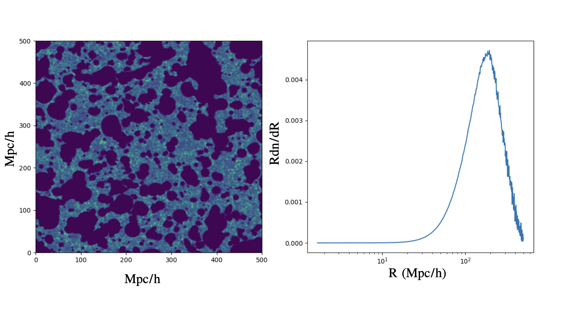
Figure 1: In the left panel, we show a slice from a grizzly simulation at $z=9.1$. The solid dark regions are the completely ionized regions. This slice has a volume averaged ionized fraction of $0.40$. The plot on the right is a size distribution of ionized bubbles obtained from the ionized map using the mean-free-path method.

2.2 Modeling the 21-cm signal with grizzly

In this paper, we use the one-dimensional radiative transfer code, grizzly [57, 58] to model the 21-cm signal. The algorithm uses uniformly gridded dark-matter density cubes and their corresponding dark-matter halo-lists, along with the velocity-field cubes as inputs. Given a source model, grizzly then generates the ionization maps and the brightness temperature maps during the EoR. In our models, we assume $T_{s}\gg T_{\gamma}$, which is expected to be the scenario in the presence of efficient X-ray heating [see e.g, 59, 60, 61, 62]. This implies that the large-scale fluctuations of the signal are mostly driven by density and ${\rm x}_{\rm HI}$ fluctuations. For this paper, the simulations considered use the gridded dark-matter density fields and the corresponding halo lists within comoving cubes of side 500 $\mathit{h}^{-1}$ Mpc, produced from the PRACE4LOFAR N-body simulations (for the details of the simulation, see e.g, [63, 64]). We vary the following parameters, which control the source models to generate a suite of simulations:

1. Ionization efficiency $\zeta$: The rate of ionizing photons per unit stellar mass, escaping from a halo is given by, $\dot{N_{i}}=\mathrm{\zeta\times 2.85\times 10^{45}~{}s^{-1}~{}M_{\odot}^{-1}}$. Here, $\zeta$ is the ionization efficiency. The rate of ionizing photons is assumed to be proportional to the halo mass and the ionizing efficiency, $\zeta$ combines the degeneracies from other astrophysical parameters (such as the star formation rate, the emission rate of ionizing photons from the sources, as well as their escape fraction) in the IGM.

2. Minimum mass of the UV emitting halos ${M_{\mathrm{min}}}$: The number of ionizing photons escaping from a halo is assumed to be linearly dependent on its mass. However, below a certain minimum mass, radiative and mechanical feedback can severely reduce the star formation efficiency [65, 66]. We thus introduce ${M_{\mathrm{min}}}$, which is the minimum mass of the halos, from which ionizing photons escape into the IGM.

For a set of source parameters $\bm{\theta}=[{\zeta,M_{\mathrm{min}}}]$ and the previously described inputs from the N-body simulation, grizzly first generates ionization maps at the given redshift. These ${\rm x}_{\rm HII}$ maps are later used to produce coeval $\delta T_{b}$ maps using Eq. 2.1. Note that we use the cell moving technique [67, 68] to include the impact of the redshift space distortion.

2.3 Characterizing the IGM

Most EoR simulations are dependent on the source parameters, a combination of which can be used to generate several reionization scenarios. However, as the 21-cm signal is a more direct probe of the state of the IGM, we choose to characterize the IGM with the following parameters.

1. The volume-averaged ionization fraction, $\overline{{\rm x}}_{\rm HII}$: As the Universe transitioned from a predominantly neutral state to an ionized state, the ionized regions gradually began to grow in size. This led to the formation of a network of ionized regions, with ionized bubbles surrounding dense regions hosting ionizing sources. The volume-averaged ionization fraction, $\overline{{\rm x}}_{\rm HII}$ provide a measure of the ionization state of the Universe, at a certain redshift.

2. The bubble size distribution (BSD): The size distribution of regions containing ionized Hydrogen during the EoR is an important quantity which can encapsulate crucial insights about early stars and galaxy formation. At a given redshift, the tomography of the IGM can be best described by such a size distribution. The BSD describes the range of sizes that these ionized regions can have, and their relative abundances. There are a few methods of determining the size distribution of the bubbles, for example, the Friends-of-Friends (FoF) method and the Mean-Free-Path (MFP) method. The FoF method is based on the percolation theory and works well when there are only bubbles of equal sizes, focussing on the connectedness of the ionized regions. The FoF method is computationally very expensive and fails when there are bubbles of different sizes, particularly in the later stages of reionization when there are several overlapping ionized regions. In this work, we use the MFP method to determine the size distribution of the bubbles. To obtain a bubble size distribution from a simulation, a pixel within an ionized region is randomly chosen, and the distance from this point to the nearest neutral pixel in a random direction is measured and recorded. This procedure is repeated several times $(\sim 10^{7}$ times), and these distances are recorded, following which a probability distribution function (PDF) of these distances is obtained. The bubble size distribution can be derived by taking the volume-weighted average ([69]) of the probability distribution function. The PDF is given by $\mathrm{R\frac{dn}{dR}}$, where, n denotes the number of recorded lengths or rays or mean-free-paths, in the range from $\mathrm{R}$ to $\mathrm{R+dR}$. In Fig.1, we show a slice from a grizzly simulation with a volume averaged ionization fraction of $\sim 40\%$. The right-hand panel of the figure shows the corresponding bubble size distribution. It should be noted that as a direct implication of the fact that Gaussianity is driven by large number statistics, the mean of the distribution is driven by the bubbles at larger scales.

These IGM parameters are derived quantities, and are very informative in characterizing the state of the IGM at a specific redshift. Nonetheless, while considering the dynamic evolution of the IGM over a range of redshifts, additional parameters would be important to comprehensively capture its characteristics.

3 Artificial Neural Networks

In this section, we describe the methodology to develop our ANN-based framework that connects the IGM-related quantities to the 21-cm signal power spectrum. We describe the basic architecture of the ANN and elaborate on the details of how the training and test datasets were created to develop our framework.

3.1 Brief overview of ANN

Artificial Neural Networks (ANN) are one of the several available machine learning techniques which can be used for developing supervised learning-based frameworks. A neuron is the functional unit of an ANN. A basic neural network has three kinds of layers: an input layer, one or more hidden layers, and an output layer. In a fully connected network, each neuron in a layer is connected with every neuron in the next layer, and the connection is associated by a weight and a bias. ANNs are capable of mapping associations with a given input data and associated target parameters of interest, without the knowledge of their explicit causal relationships. During the training process, the network gradually optimises a chosen cost function by repeatedly back-propagating the errors and adjusting the weights and biases. A chunk of the data is put aside as the validation dataset and the performance of the network is validated using this set. For a detailed description of a similar training process, please see [44]. Once training and validation are completed, a test set is used to check the robustness of the network and predict the output parameters. For a detailed mathematical description of how the weights and biases are adjusted for every iteration, see [70], also summarized in [44].

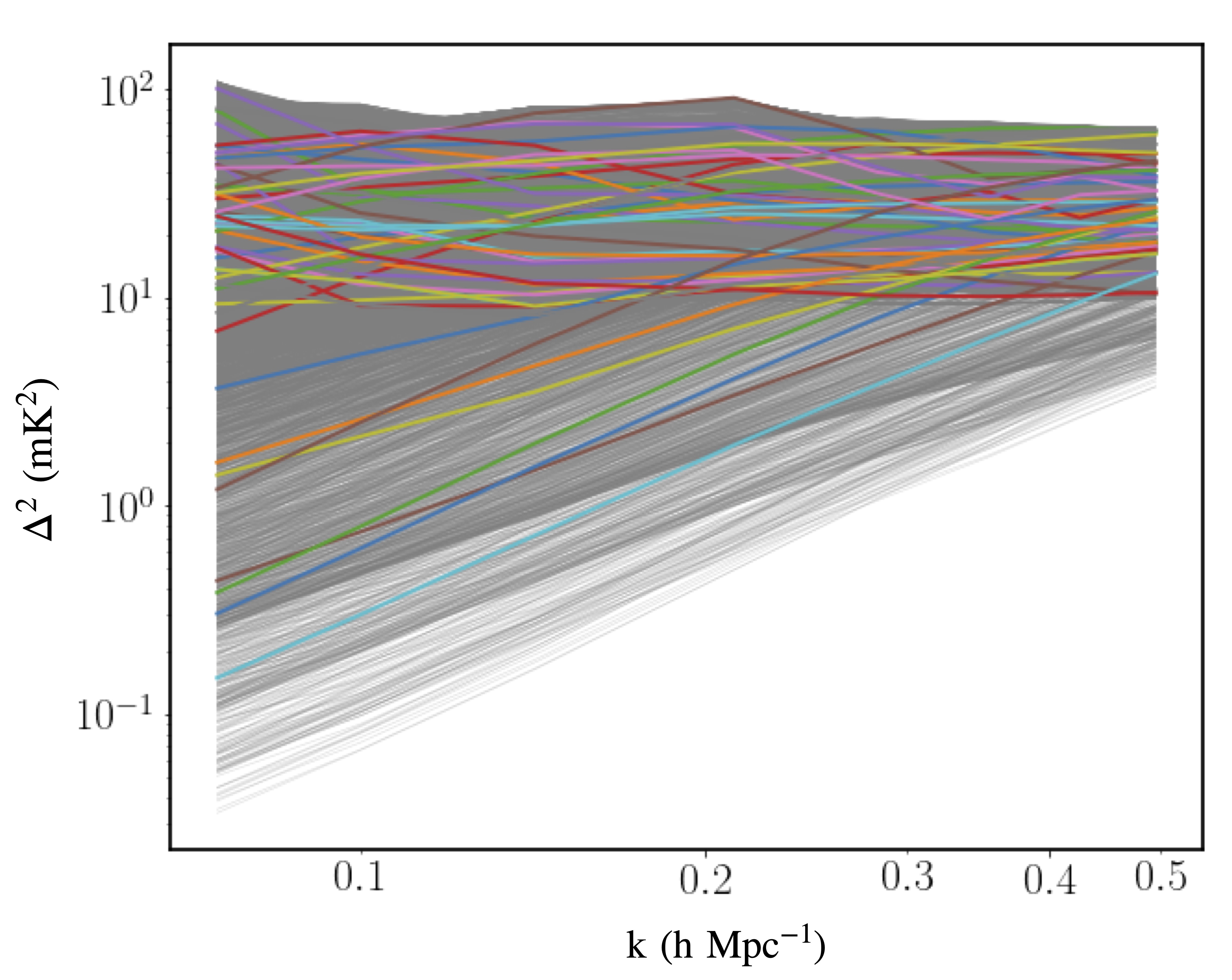
Figure 2: This is the power spectrum set consisting of 17000 models used for training the ANN. In this plot, a fraction of the training set is plotted in color, while the rest have been plotted in grayscale, to provide an idea of the different shapes of the power spectra included in the training set.

Training of ANN in a supervised manner is very target-specific, and can have very different network architectures for different applications. While ML methods are extremely fast and computationally very efficient, the ANN model performances need to be carefully analysed. There can be issues of “overfitting”, which is typically the case when the trained model fails to generalize what it has learned during the training process. Such a scenario can be overcome by suitable regularization techniques. There can also be an “underfitting” scenario, which can be identified if the training error does not reduce even after several iterations. This can also be solved by making the network more complex (e.g: by adding more layers) and also by using a well-represented training dataset.

Once the ANN is trained, validated and tested, one requires to define a metric to quantify the performance and robustness of the network. There are various available metrics which can be computed to provide a quantification of the performance of the ANN, of which the most commonly used metrics for supervised learning methods are RMSE (root mean squared error) and R2 score (also called the coefficient of determination), which provide a measure of error in the predictions of the ANN. In this paper, we compute R2-scores for each of the output parameters as the performance metric. The R2-score is defined as:

$$\mathrm{R^{2}=1-\frac{\Sigma(y_{pred}-y_{orig})^{2}}{\Sigma(y_{orig}-\overline{y}_{orig})^{2}}}$$ (3.1)

where, $\mathrm{{y}_{orig}}$ is the original parameter, $\mathrm{y_{pred}}$ is the parameter predicted by the ANN, $\mathrm{\overline{y}_{orig}}$ is the average of the original parameter, and the summation is over the entire test set. $\mathrm{R}^{2}$ can vary between 0 and 1, while $\mathrm{R}^{2}=1$ implies a perfect inference of the parameters.

3.2 Preparing the training and test sets for the 21-cm PS emulator

We have used publicly available python-based packages scikit learn ([71]) and keras in this work to design the networks. In this paper, we use two separate sets of simulations.

• Training set I: In our effort to span most of the parameter-space of the IGM and various shapes of the 21-cm power spectrum, we modify the source model described in §2.2. We describe a source model in which the rate of ionizing photons escaping from a halo is given by, $\dot{N_{i}}=\mathrm{\mathcal{A}\cdot\mathcal{M}_{halo}^{\alpha}}$. Here, $\mathrm{\mathcal{A}}$ is a proportionality constant, which includes other source parameters and $\alpha$ determines the non-linear dependency of the number of ionizing photons on the mass of the halo. This aims to encompass various scenarios of reionization, incorporating different morphologies that could result in different size distributions. By choosing a value of $\alpha\in(-2,2)$ and the ionized fraction of the IGM, ${\rm x}_{\rm HII}\in(0.20,0.90)$, we generate a large number of different scenarios at redshift $z=9.1$ (Fig.2). To avoid any bias in our training set due to over-representation of any particular ${\rm x}_{\rm HII}$, we ensure that ${\rm x}_{\rm HII}$ is sampled uniformly in the range $\in(0.20,0.90)$, resulting in $\sim 17000$ models which we use to construct the training set. Thus, our training dataset comprises of the ionized fraction and the normalized bubble size distribution for each of the model, and the corresponding 21-cm power spectra. We generate a test set consisting of 1466 samples following the same method, and call it the grizzly test set. This training set is used to train the emulator (ANN-Emu) (§ 4.1) and the ANN for the IGM parameter estimation (ANN-IGMParam) (§ 4.3).

• Training set II: The second set of training samples is generated using the source model as described in section § 2.2. We use simulations with a box size of $\rm 500~{}\mathit{h}^{-1}\mathrm{Mpc}$ and compute the corresponding 21-cm power spectra, bubble size distributions and the volume averaged ionization fraction for each model. We also record the source parameters for this set, which we use later in §4.4. This set is smaller in size, comprizing of $\sim 4000$ samples. This training set is used to train an ANN to determine source properties $[\rm\zeta,M_{min}]$ directly from the IGM properties $[\mathrm{BSD,\overline{{\rm x}}_{\rm HII}}]$ (ANN-Source), which we discuss in detail in § 4.4.

We describe the architecture and the results from the ANN emulator and parameter estimation in the following section. We have summarized the different ANNs, their target and their corresponding training set in Tab.1.

ANN name	Description	Training set
ANN-Emu	Emulator to predict 21-cm PS from BSD and $\overline{{\rm x}}_{\rm HII}$	Training set I
ANN-IGMParam	IGM Parameter estimation, $[A,\mu,\sigma,\overline{{\rm x}}_{\rm HII}]$ from 21-cm PS	Training set I
ANN-Source	Source parameter estimation, $[\rm\zeta,M_{min}]$ from $[A,\mu,\sigma,\overline{{\rm x}}_{\rm HII}]$	Training set II

Table 1: List of the different ANNs and their corresponding training sets

4 Results

We describe our results in this section. Firstly, we present the results from the ANN emulator(ANN-Emu) for grizzly test set. This emulator is implemented into a Bayesian framework to constrain the IGM parameters. Subsequently, we present the results of IGM parameter estimation using a trained ANN, and compare the results with the Bayesian framework. We further use noisy test datasets corresponding to 1000 hours of observation of the SKA-low configuration to predict the IGM parameters. Finally, we determine the source parameters from the IGM parameters using an ANN.

4.1 Predictions of the 21-cm power spectra from grizzly test sets

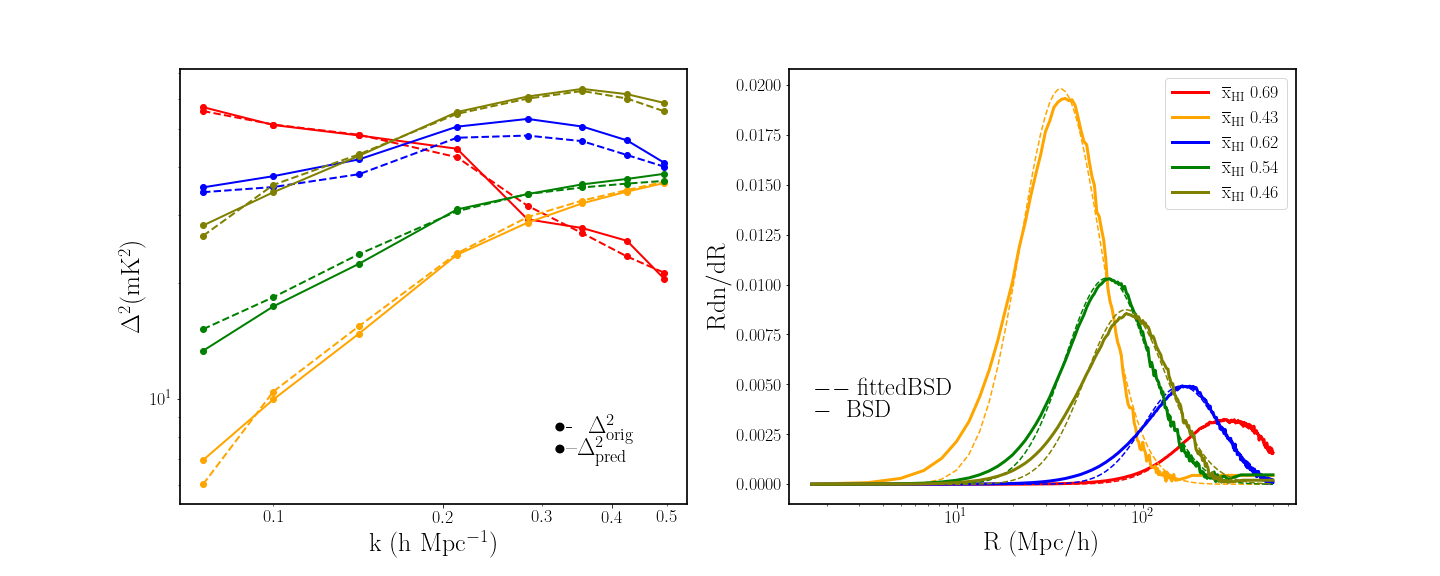
Figure 3: The panel on the left side shows the predictions of the ANN, from a random subset of the test set which comprises of grizzly models at redshift 9.1. The plot shows the true and the predicted power spectra from the ANN emulator, represented by the solid and the dotted curves respectively. The solid curves on the right show the corresponding BSD and their ionization fractions. The dashed curves on the right panel are the log-norm fitted BSDs.

For the ANN emulator, we use a Multilayer-perceptron based ANN with 4 hidden layers, and activation functions ‘elu’ for each of hidden layers. The number of input neurons corresponds to the dimension of the input dataset, which is 301 in our case (300 for the BSDs and 1 for the $\overline{{\rm x}}_{\rm HII}$, per realization). The output layer has a linear activation function, and provides the 21-cm power spectrum for a range of $\mathit{k}$-values as the output.

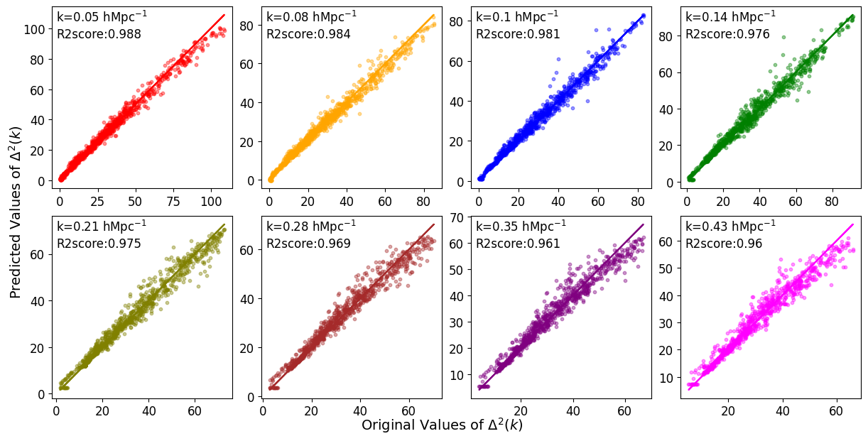
Figure 4: The true versus predicted values from the grizzly test set from ANN-Emu, for each k-mode along with their R2 scores are shown in this figure.

To assess the performance of the ANN emulator, we first consider the grizzly test set which contains 1466 samples. Given a BSD, along with its ionized fraction at redshift 9.1, the emulator is trained to predict the 21-cm power spectrum for the $\mathit{k}$-modes [0.05, 0.08, 0.1, 0.14, 0.21, 0.28, 0.35, 0.43] $\mathrm{\mathit{h}Mpc^{-1}}$. In Fig.3, we show the predictions from the ANN emulator for a fraction of the test set consisting of models using the grizzly simulation (or the grizzly test set). In the right panel of the same figure, we plot the corresponding BSD along with the ionized fractions (mentioned in the legend). In order to better demonstrate the accuracy of predictions from our ANN model, we present scatter plots of the $\mathrm{\Delta^{2}_{pred}}$ versus $\mathrm{\Delta^{2}_{true}}$ per k-bin with the corresponding R2-scores in Fig.4, where $\Delta^{2}$ is the dimensionless power spectrum and the subscripts "true" and "predicted" denotes the true 21-cm power spectrum and the predicted 21-cm power spectrum respectively. If we plot the distribution of the ratio of true versus predicted power spectra per k-bin (see Fig. 5, we observe that, for more than $95\%$ of test set samples, the distribution is centered around 1.

From the scatter plots in Fig.4, we see that the R2-scores from the predictions for different $\mathit{k}$-values are between $0.898-0.978$. An R2-score closer to 1 implies a very good prediction. We also observe that at higher k-values $\mathrm{(\mathit{k}>0.08~{}\mathit{h}Mpc^{-1})}$, the R2-score is not as good as the two lowest $\mathit{k}$-modes we consider in this work. These comparatively less accurate predictions at the larger k-values corresponding to smaller angular scales, could be due to much more noisy information at those scales. Although the BSD is a reasonably good statistical representation of the distribution of the sizes of the ionized bubbles, there is some information lost while transitioning from the ionized maps to the size distributions, particularly in scenarios where there are complex shaped, overlapping structures in advanced stages of reionization. Also, the BSD does not give us complete information about the location and extent of the bubbles, which translates to a complicated mapping between the BSD and the 21-cm power spectrum. Combining all these points, the emulator is slightly less accurate in predicting the power spectra at higher k-modes. We will be incorporating this emulator in the following section to obtain Bayesian constraints on the IGM parameters.

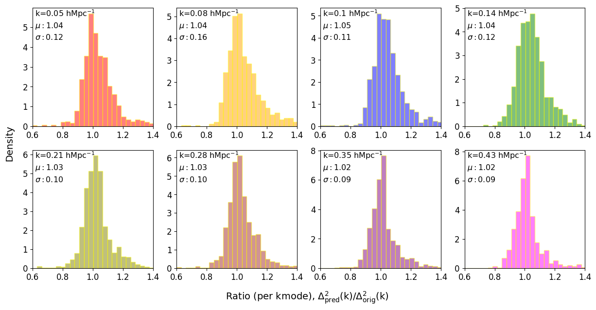
Figure 5: The ratio of the true versus the predicted values from the grizzly test set for each k-mode are shown in this figure, along with the mean $(\mu)$ and standard deviation $(\sigma)$ of these distributions.

4.2 Bayesian constraints on IGM parameters using the trained ANN model

For a given model, placing robust and quantitative constraints on the model parameters (given a series of observations and their associated uncertainties) is the basic motivation of parameter inference. A posterior probability distribution $\mathcal{P}(\theta|x)$ of the model parameters, $\theta=\{\theta_{1},\theta_{2},...,\theta_{n}\}$, given a data vector, $x=\{x_{1},x_{2},...,x_{n}\}$, is usually computed following Bayes’ theorem:

$$\mathcal{P}(\theta|x)=\frac{\mathcal{L}(x|\theta)\pi(\theta)}{P(x)},$$ (4.1)

where, $\mathcal{L}$ is the likelihood function of the data, $\pi(\theta)$ is the prior probability distribution of the model parameters, and $P(x)$ is the probability distribution of the given data. The maximum likelihood estimate is found by maximizing $\mathcal{L}(x|\theta)$, and the maximum a posteriori estimate is computed by maximizing $\mathcal{P}(\theta|x)$. This entire process works well as long as the parameter space is not very vast, and the parameters themselves are also well-behaved.

In this subsection, we present the Bayesian constraints on the IGM parameters. We do so, by using the ANN emulator (described in detail in § 4.1), which has been trained to predict the 21-cm power spectrum from a given bubble size distribution and the ionized fraction. If we directly use the ANN-emulator as the model for Bayesian inference, we would require 301 parameters in total, corresponding to the number of inputs that goes into the ANN (the first 300 corresponding to the BSD and one corresponding to the ionized fraction). That would result in a very large number of parameters to constrain. To avoid this, we opt for a simpler parametrization of the bubble size distribution as a log-normal distribution (Eq.4.2), where, A, $\mu,\sigma$ are, respectively, the amplitude, mean and standard deviation of the corresponding normal distribution; and r is an interpolated, equally spaced array corresponding to the size of the box in units of $h^{-1}\rm{Mpc}$, given by:

$$\mathrm{BSD\mathrm{(}A,\mu,\sigma,r)}=\mathrm{\dfrac{A}{r\sigma\sqrt{(}2\pi)}\exp\left(-\dfrac{1}{2}\dfrac{(\log(r)-\mu)}{\sigma}^{2}\right)}$$ (4.2)

It should be noted that this parametrization is the best possible representation of the BSD though it is not an absolutely perfect fit. As there can be different size distributions corresponding to same volume averaged ionization fractions, it is not straightforward to uniquely map a power spectrum with a log-normal parametrized BSD and $\overline{{\rm x}}_{\rm HII}$.

We implement a hybrid approach to obtain constraints on the IGM parameters using a Bayesian method as well as an ANN. First we set up our ANN emulator to predict the 21-cm power spectrum, given the bubble size distribution and the ionized fraction (as described in the §3.2). Following this, we employ our power spectrum emulator to a Bayesian sampler, the emulator allows us to avoid a direct dependence on the semi-numerical simulation, thus making this process computationally fast. The final output of the sampler is the posterior probability distribution for the parameters. We report the mode or the most probable value for each of the parameters from the marginalized distributions as the predicted value and calculate the uncertainty bound based on the quantiles. In this work, we implement the ANN emulator into the standard Markov Chain Monte Carlo (MCMC) based parameter estimation method for our data. We use the publicly available code EMCEE to obtain constraints on the 4 IGM parameters, $\rm A,\mu,\sigma,\overline{{\rm x}}_{\rm HII}$. Fig.6 shows the posteriors obtained and the pair-wise covariances of the IGM parameters for an input 21cm power spectrum which corresponds to an ionaization fraction of $0.32$ alongwith $20\%$ noise. We obtain good constraints with the combination of Bayesian methods along with the trained ANN-emulator.

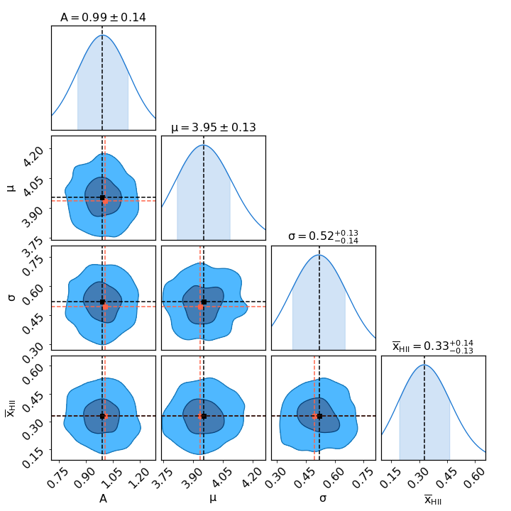
Figure 6: The posterior distributions of the IGM parameters, $A,\mu,\sigma$ (corresponding to the BSD) and $\overline{{\rm x}}_{\rm HII}$. The off-diagonal terms show the pair-wise covariances and the diagonal plots show the marginalised distributions. The 2D contour levels represent the $1\sigma$ and $2\sigma$ levels of probability. The shaded regions in the margialized distributions depict the $68\%$ probability range. The black and orange dashed lines represent the mean values of the posterior distribution and the true values of the parameters respectively.

4.3 ANN for parameter estimation

While we obtain reasonable constraints on the IGM parameters from our Bayesian analysis, we bring to note that not all BSD’s can be perfectly parametrized by a log-lognormal distribution. Hence the scope of introducing an error in our estimation already stems from the choice of the parameters for the size distributions.

In this subsection, we present an ANN-IGM parameter estimator, which is trained on the same training set as described in § 3.2. This ANN is also a multilayer perceptron network, with two hidden layers, each with an activation function ‘elu’. The input layer has 8 neurons corresponding to the input 21-cm power spectrum. The output layer has four parameters, three corresponding to the BSD parameters $(A,\mu,\sigma)$ and the volume-averaged ionization fraction $\overline{{\rm x}}_{\rm HII}$. Given the 21-cm power spectrum, we can use this ANN to predict the IGM parameters that describe the EoR.

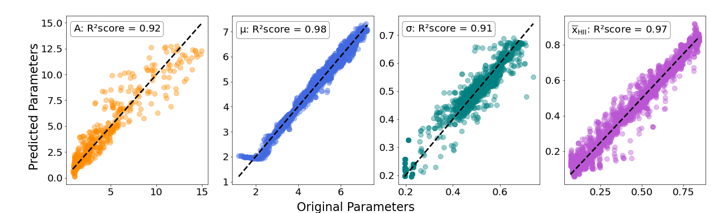
Figure 7: Results from the ANN-IGM parameter estimator, which is trained to predict the IGM parameters (the BSD parameters $A,\mu,\sigma$ and the ionization fractions $\overline{{\rm x}}_{\rm HII}$), given the 21-cm power spectrum. The plots of the true vs predicted values for each of the IGM parameters are shown. The black line in each plot represents the true values. The respective R2 scores are mentioned in the top-left-hand corner of each plot.

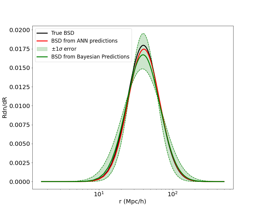
Figure 8: The reconstructed bubble size distributions from the predicted BSD parameters obtained from Bayesian method (green) along with the $1\sigma$ error limits and ANN method (red). The black curve is the BSD with the original parameters.

Parameter	True values	Bayesian method	ANN method
$\mathrm{A}$	1.008	$\mathrm{0.99}^{+0.14}_{-0.14}$	0.999
$\mathrm{\mu}$	3.935	$\mathrm{3.95}^{+0.13}_{-0.13}$	3.954
$\mathrm{\sigma}$	0.493	$0.52^{+0.13}_{-0.14}$	0.495
$\overline{{\rm x}}_{\rm HII}$	$0.329$	$0.33^{+0.10}_{-0.13}$	0.312

Table 2: A comparison of values of the IGM parameters obtained from the Bayesian and ANN methods, along with the true values. This is one example for comparing the predictions using ANN and Bayesian methods. We find that the ANN based estimator outperforms the Bayesian methods, even though the ANN predictions do not come with error contour levels. The corresponding reconstructed BSDs are shown in the Fig.8.

To demonstrate the performance of the ANN-IGM parameter estimator, we have two test sets:

1. Predictions of the IGM parameters from noise-free grizzly test sets
   This test set consists of a set of 21-cm power spectra from the grizzly simulations. Given any 21-cm power spectrum, the ANN predicts the corresponding BSD parameters $(A,\mu,\sigma)$ and $\overline{{\rm x}}_{\rm HII}$. We have shown the original versus the predicted values of the parameters from the grizzly test set, in Fig.7. The R2-scores of the parameters for $A,\mu,\sigma,\overline{{\rm x}}_{\rm HII}$ are 0.92, 0.98, 0.91, 0.97 respectively. We observe that the parameter A, which corresponds to the amplitude of the BSD not as well constrained as the other parameters.

   In Tab.2 we compare the predictions obtained from the ANN with the results obtained from the Bayesian analysis. While the ANN takes $0.012$seconds to predict the parameters, the standard Bayesian MCMC method takes $64.457$minutes to converge on a personal computer with 8 cores and 16GB memory. We find that the results are comparable to the true values of the parameters. Once we have the predicted values of the BSD parameters from the ANN, we use them to reconstruct the BSD using Eq.4.2. In Fig.8, we show the reconstructed bubble size distributions using the predicted parameters from both methods, along with shaded region showing the $1\sigma$ error on the Bayesian predictions.

2. Predictions of the IGM parameters from test sets with SKA noise
   We consider a more realistic test set, which contains a set of 21-cm signals contaminated with SKA thermal noise. We use the publicly available code 21cmsense([72, 73]), to generate the sensitivities corresponding to SKA1-low. The sensitivity of an instrument indicates the ability of the instrument to detect the faintest signal possible. In the method followed in 21cmsense, a uv coverage of the observation is generated by gridding each baseline into the uv plane and including the effects of the Earth’s rotation over the course of the observation.

   The upcoming SKA telescope would possess sufficient signal-to-noise required to detect the statistical 21-cm signal ([20]) and also perform 21-cm tomography ([74]). With 38 m diameter corresponding to a collecting area of $\sim 600~{}\mathrm{m}^{2}$, SKA1-low will have a field of view of about 12.5 $\mathrm{deg^{2}}$ at 150 MHz. The full SKA1-low configuration will extend up to a diameter of approximately 40 km spread around the core and the longest baseline would be about 65 km. In our calculations, we have used 224 core elements spread within a radius of 500 m. The shortest and longest baseline of the core is 35.1 m and 887 m, respectively. This results in an angular resolution of $10^{{}^{\prime}}$ at 150 MHz. We have obtained the thermal noise power spectra for these experiments corresponding to a total of 1080 hours of observation for SKA (in 6 hours of tracking mode observation per day, for 180 days). Using these thermal noise power spectra, we generate the SKA-noise test set samples.

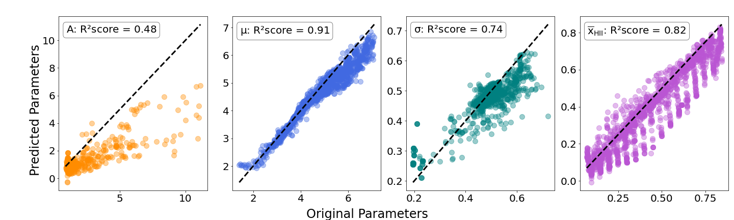
Figure 9: In this figure, we show the scatter plots of true versus predicted IGM parameters $A,\mu,\sigma,\overline{{\rm x}}_{\rm HII}$ from the SKA-noise test sets. In the top left-hand corner of each plot, we mention their R2-scores respectively.

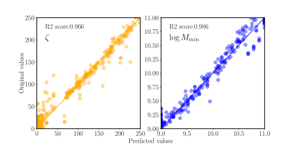
Figure 10: Results of the ANN trained to predict the source parameters from the bubble size distribution and the ionization fractions, given the 21-cm power spectrum. The plots of the true vs predicted values for each of the parameters are shown.

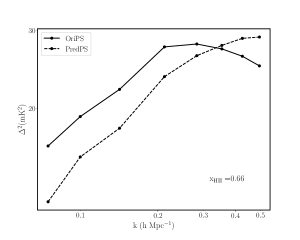
(a)

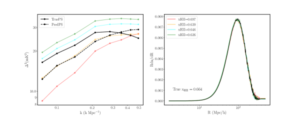
(b)

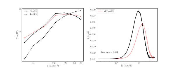
(c)

Figure 11: A crude representation of how crucial a unique mapping of the BSDs and $\overline{{\rm x}}_{\rm HII}$ parameters are to the 21-cm power spectrum in the training set. Here we show one test set sample from c2ray simulations. In the first plot, we show the true versus predicted 21-cm power spectrum of the sample from the c2ray test set. In the second panel, we see that even though the BSD is quite close to the samples we have trained the ANN with, the corresponding $\overline{{\rm x}}_{\rm HII}$ and the 21-cm power spectra are very different. This does not allow the ANN to predict the 21-cm power spectrum as accurately as expected. In the third panel, we search for a power spectrum that is closest to the test power spectrum and plot it. We observe that the corresponding BSD and $\overline{{\rm x}}_{\rm HII}$ is very different from the BSD of the c2ray sample.

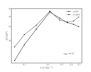
(a)

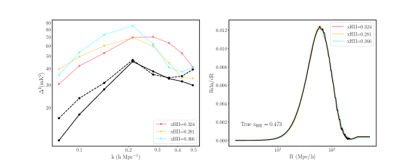
(b)

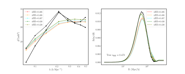
(c)

Figure 12: A crude representation of how crucial a unique mapping of the BSDs and $\overline{{\rm x}}_{\rm HII}$ parameters are to the 21-cm power spectrum in the training set. Here we show an example from the 21cmfast simulations. In the first plot, we show the true versus predicted 21-cm power spectrum of a sample from the 21cmfast test set. In the second horizontal panel, we see that even though the BSDs are close to the samples we have trained the ANN with, the corresponding ionization fractions, ${\rm x}_{\rm HII}$ are different. This does not allow the ANN to predict the 21-cm power spectrum as accurately as expected. In the third panel, we search for a power spectrum that is closest to the test power spectrum and plot it. We observe that the corresponding BSD and $\overline{{\rm x}}_{\rm HII}$ are very different from what we provide as an input.

In Fig.9, we show the original values versus predicted values of each of the IGM parameters from the SKA test sets. We see that the R2-scores are lower than the test set without any SKA-noise. The R2-scores for $A,\mu,\sigma,\overline{{\rm x}}_{\rm HII}$ for SKA test sets are respectively 0.48, 0.91, 0.74, 0.82. We observe that when input 21-cm power spectrum is contaminated with SKA noise, the ANN is not able to accurately predict the BSD parameters accurately. However,in comparision there is a smaller effect on the prediction of the volume-averaged ionization fraction from the SKA test set. It should be noted that the ANN-IGM has not been trained on the noisy data.

4.4 Determining the source properties from the IGM properties

The 21-cm power spectrum is a measurement of the state of the IGM. This in turn does depend on the source parameters but this dependency is indirect and different source parameters may produce similar IGM states. Nevertheless, it is not self-evident how to best parametrize the state of the IGM. Several recent works (e.g.,[37]) have focused on constraining the source parameters from power spectrum measurements. We would like to stress on the fact that the 21-cm power spectrum has a direct connection with the state of the IGM. Evidently, there is an interplay of several different factors which is neither captured directly by the power spectrum nor can be completely described by the current state of parameters characterizing the IGM. In this paper, we use the size distribution of the ionized regions and the volume-averaged ionization fraction of the IGM as the primary parameters to describe the IGM, assuming no spin temperature fluctuations at redshift 9.1. If we extend our formalism to other redshifts, and include spin temperature fluctuations, heating and feedback effects, then the parameter set describing the IGM would be much larger and complicated.

As we demonstrated the IGM parameter estimation in the previous sections, we now would like to understand if it is possible to retrieve the source parameters from these IGM parameters directly in the simplest scenario. This framework will be useful if we are able to infer the IGM parameters from an observed 21-cm power spectrum, and would want to understand the nature of the associated source parameters directly from them. We could then compare the inferences about the source parameters from other methods which directly use the 21-cm power spectrum and understand the nature of the sources in a more comprehensive way.

For this task, we train another ANN (we refer to as ANN-Source) which takes the IGM parameters as inputs and predicts the source parameters. We use a multilayer perceptron model of ANN which has $301$ neurons in the input layer corresponding to the IGM parameters $(\rm BSD,\overline{{\rm x}}_{\rm HII})$, followed by three hidden layers with activation functions of ‘elu’.The output layer has two neurons, corresponding to the two source parameters, minimum mass of halos $\mathrm{\log M_{min}}$ and ionizing efficiencies, $\zeta$, which are most relevant for reionization. We use a training set comprising of 7680 samples and train an ANN to predict $(\mathrm{\log M_{min}},\zeta)$, given the BSD and the $\overline{{\rm x}}_{\rm HII}$ at redshift $z=9.1$. Fig.10 shows the scatter plot of the true versus predicted values of the source parameters that we obtain from the trained ANN-model. The R2-scores corresponding to the parameters $\mathrm{\log M_{min}}$ and $\mathrm{\zeta}$, are $0.966$ and $0.986$ respectively, which imply that the predictions are quite close to the original/true values. This is for the first time that we demonstrate such a non-analytical association between the IGM quantities and the source parameters using ANN. Our results suggest this may be interesting to explore further for example for different source models.

5 Discussions

The parameter space for the EoR is quite large, and we still do not know with certainty what would be the best set of parameters which would most closely describe the state of the IGM. This is a very difficult task, especially because of the dynamic nature of the evolution of the IGM, which is in turn affected by several unconstrained astrophysical and reionization parameters. Hence, simulation based parameter inference methods (analytical, numerical or ML based) become dependent on the choice of the parameter space, source models and the models of reionization considered.

We have considered the BSD and $\overline{{\rm x}}_{\rm HII}$ as the parameters to describe the IGM. One of the primary concerns of using a BSD to describe the state of the IGM is the fact that it does not work well in scenarios where there are overlapping bubbles or irregularly shaped ionized bubbles. As the method of defining the bubble size distribution using the mean-free path method is somewhat incomplete (as it does not take into consideration the information of the locations and the shape of the bubbles), it becomes difficult to completely and accurately represent the distribution of the ionized structures.

The most crucial aspect of implementing supervised learning methods in ML is the choice of the training set. The training set needs to be chosen in such a way that it sufficiently represents all possible reionization scenarios which we want our network to learn about. While this is quite straightforward and simulation model dependent, when one considers designing an emulator to map ’controllable’ EoR source parameters to the 21-cm power spectrum, it becomes slightly complicated while we try to map the derived IGM parameters to the 21-cm power spectrum. As different kinds of morphologies can result in the same volume averaged ionization fraction, there is no unique mapping between a combination of a given size distribution and the volume averaged ionization fraction, and the associated 21-cm power spectrum. This also makes it complicated to have an ideally uniformly sampled input parameter space. In this work, we included several possible reionization scenarios leading to various shapes of power spectra. For the ANN emulator, the input parameter space is comprised of the corresponding BSD and $\overline{{\rm x}}_{\rm HII}$ and the target space consists of the the 21-cm power spectra. This work demonstrates the training of an ANN with a combination of a continuous distribution(BSD) and discrete ($\overline{{\rm x}}_{\rm HII}$) values in the input parameter space.

Another common issue with ML methods when used with simulations, is the problem of generalizability. We observe that in supervised learning methods, the ANN performs poorly, if the test sets are derived from an entirely different simulation. This could be due to the underlying differences in the implementation of the physics models and various other details and approximations.

To test how well the emulator could predict the 21-cm power spectrum from a test set which is not generated by the grizzly simulation, we use the simulations from the 3D RT code, c2ray. In this example, we take a particular sample from the c2ray test set and input its IGM parameters, BSD and $\overline{{\rm x}}_{\rm HII}$ to obtain the predicted 21-cm power spectrum. In the top centre plot in Fig.11, we show true versus predicted 21-cm power spectra using the c2ray test set. In the following two horizontal panels, we demonstrate how the absence of similar models in the training set affects the prediction from the ANN for the power spectrum plotted in pink. In the second row plots, we look for the closest match between the test set c2ray sample and the samples in the training set. We find that there are a few BSDs which match the c2ray BSD with a $\chi^{2}\sim 10^{-7}$. Plotting only the BSDs which have ionization fractions in between $0.60-0.70$, we observe that these BSDs correspond to quite a large range of shape and amplitudes in the 21-cm power spectrum space, particularly towards the lower $\mathit{k}$-modes. For the third row of plots, we search for a similar shape of the 21-cm power spectrum from our training set and find that the closest match available has a corresponding $\chi^{2}\sim 0.02$, but the BSD and $\overline{{\rm x}}_{\rm HII}$ of that particular case is very different from the c2ray sample being considered.

We show another similar test case, using a test set sample from the seminumerical simulation, 21cmfast in Fig.12. We find that there is no sample in our training set which represents the kind of power spectrum that is expected from the 21cmfast test set sample. This implies that each of the simulations have very different approximation techniques and non-generalizable models which plays a crucial role in determining the distribution of ionized sources and the power spectrum.

To make the training set most diverse , we incorporated different shapes of the 21-cm power spectrum corresponding to the c2ray models in our training sets. We observed that even if we are able to match the shape of the power spectrum by making the ionization model more extreme by using a different power-law model (for example, using higher values of $\alpha$, as discussed in § 3.2), the corresponding BSDs are not similar to those obtained from grizzly. We demonstrate the crucial association of the IGM parameters, the BSD and $\overline{{\rm x}}_{\rm HII}$ with the shape of the power spectrum in Fig.11 and Fig.12. We realize that our training set is not sufficient to work seamlessly for test set samples from other simulations which use drastically different models as compared to grizzly. We plan to incorporate more diverse models and develop a generalizable and complete training set in our future work.

Another important point which should be noted is the completeness of the IGM parameter set that has been considered in this work. While the BSD and $\overline{{\rm x}}_{\rm HII}$ does a fairly good job of describing the power spectrum, we are limited to one kind of simulation only (grizzly, with a specific kind of source model as discussed in detail in earlier sections). Our ANN emulator is not accurate when we try to test it on other kind of simulations which have their respective source models, parameters and assumptions. It is important to understand that the grizzly-trained network is not successful in inferring the IGM parameters from the 21-cm signal from different simulations, possibly due to different algorithms used in these codes. This could imply that any interpretation of future 21-cm results could be code-dependent, which is a matter of concern. It is important to consider cross-collaborating between different code groups and arrive at a standardized parametrization which would enable us to switch between different codes and incorporate them in our inference frameworks. We are exploring novel methods to incorporate a wide variety of size distributions and different shapes of the 21-cm power spectrum, for future work.

6 Summary & Conclusions

In this paper, we present a new ANN based machine learning framework to extract the IGM parameters from the redshifted EoR 21-cm power spectrum for the first time. We have simulated 21-cm power spectra at redshift $z=9.1$, using grizzly, which is a 1D RT code. We have covered two different aspects. Firstly, we have designed an ANN emulator using simulations from grizzly, which predicts the 21-cm power spectrum at redshift 9.1, given the size distribution of the ionized bubbles and the ionization fraction. Using this emulator, we have constrained the IGM parameters using a Bayesian framework incorporating the standard MCMC sampling.

Next, to assess the performance of our emulator based Bayesian framework, we have trained a different ANN for the IGM parameter estimation. We find that the results obtained from using MCMC and the ANN are quite comparable. Both these techniques for parameter estimation come with their pros and cons. The Bayesian method has the advantage of providing us with the confidence levels along with most likely values of the inferred parameters. However, this takes a considerable time. For this work, the bayesian algorithm took about 1 hours to converge on a machine with 40 cores. On the other hand, the ANN predictions take less than a second to predict. From the ANN predictions of the parameters in Fig.7, we see that the parameters $\sigma$ and $\overline{{\rm x}}_{\rm HII}$ have higher R2 scores, while $A$ and $\mu$ are not that well predicted.

However, when we test our Bayesian framework implementing the ANN-emulator for non-grizzly test sets, it does not perform well. With test set from other simulations, like c2ray and 21cmfast, the accuracy of prediction dropped drastically. The possible explanation of this could be the difference in the implementation of the source models in these simulations, and other underlying limitations and approximations. We found that the mapping between 21-cm EoR power spectra and their corresponding [BSD, $\overline{{\rm x}}_{\rm HII}$] were very different from the training set, when we considered test sets from other simulations.

In the final part of the paper, we demonstrate the use of ANN to predict the source parameters directly from the IGM parameters. We obtain very high accuracy for the predicted source parameters. Through this approach, we are able to demonstrate the feasability of an ANN method of inference of the source parameters directly from the IGM parameters.

In conclusion, using artificial neural networks in inferring IGM and source parameters is accurate and fast. Even though we are limited by the scope of the training sets in supervised learning methods, we can achieve very high accuracies in a very short timescales. In the future, we can make the training sets more informative so that it works well with any kind of simulations and becomes more generalizable. We plan to also extend this framework to include a range of redshifts spanning CD and EoR. Such a complementary approach using ML will be useful in identifying and breaking degeneracies in model selection and parameter estimation methods with regard to EoR 21-cm power spectrum.

References

- [1] M.F. Morales and J.S.B. Wyithe, Reionization and Cosmology with 21-cm Fluctuations, araa 48 (2010) 127 [0910.3010].
- [2] J.R. Pritchard and A. Loeb, 21 cm cosmology in the 21st century, Reports on Progress in Physics 75 (2012) 086901 [1109.6012].
- [3] S. Zaroubi, The Epoch of Reionization, in The First Galaxies, T. Wiklind, B. Mobasher and V. Bromm, eds., vol. 396 of Astrophysics and Space Science Library, p. 45, January, 2013, DOI [1206.0267].
- [4] A. Liu and J.R. Shaw, Data analysis for precision 21 cm cosmology, Publications of the Astronomical Society of the Pacific 132 (2020) 062001.
- [5] S.R. Furlanetto and S.P. Oh, Reionization through the lens of percolation theory, MNRAS 457 (2016) 1813 [1511.01521].
- [6] S.K. Giri, G. Mellema and R. Ghara, Optimal identification of H II regions during reionization in 21-cm observations, MNRAS 479 (2018) 5596 [1801.06550].
- [7] R. Ghara and T.R. Choudhury, Bayesian approach to constraining the properties of ionized bubbles during reionization, MNRAS 496 (2020) 739 [1909.12317].
- [8] A. Kapahtia, P. Chingangbam, R. Ghara, S. Appleby and T.R. Choudhury, Prospects of constraining reionization model parameters using Minkowski tensors and Betti numbers, JCAP 2021 (2021) 026 [2101.03962].
- [9] R. Ghara, S. Bag, S. Zaroubi and S. Majumdar, The morphology of the redshifted 21-cm signal from the Cosmic Dawn, MNRAS 530 (2024) 191 [2308.00548].
- [10] M. Zaldarriaga, S.R. Furlanetto and L. Hernquist, 21 Centimeter Fluctuations from Cosmic Gas at High Redshifts, ApJ 608 (2004) 622 [astro-ph/0311514].
- [11] S. Bharadwaj and S.S. Ali, On using visibility correlations to probe the HI distribution from the dark ages to the present epoch - I. Formalism and the expected signal, MNRAS 356 (2005) 1519 [astro-ph/0406676].
- [12] M.F. Morales, Power Spectrum Sensitivity and the Design of Epoch of Reionization Observatories, ApJ 619 (2005) 678 [astro-ph/0406662].
- [13] G. Swarup, S. Ananthakrishnan, V.K. Kapahi, A.P. Rao, C.R. Subrahmanya and V.K. Kulkarni, The Giant Metre-Wave Radio Telescope, Current Science 60 (1991) 95.
- [14] LOFAR collaboration, LOFAR: The LOw-Frequency ARray, aap 556 (2013) A2 [1305.3550].
- [15] HERA collaboration, Hydrogen Epoch of Reionization Array (HERA), pasp 129 (2017) 045001 [1606.07473].
- [16] S. Munshi, F.G. Mertens, L.V.E. Koopmans, A.R. Offringa, B. Semelin, D. Aubert et al., First upper limits on the 21 cm signal power spectrum from cosmic dawn from one night of observations with NenuFAR, A&A 681 (2024) A62 [2311.05364].
- [17] B.K. Gehlot, L.V.E. Koopmans, A.R. Offringa, H. Gan, R. Ghara, S.K. Giri et al., Degree-scale galactic radio emission at 122 MHz around the North Celestial Pole with LOFAR-AARTFAAC, aap 662 (2022) A97 [2112.00721].
- [18] MWA collaboration, The Murchison Widefield Array: The Square Kilometre Array Precursor at Low Radio Frequencies, pasa 30 (2013) e007 [1206.6945].
- [19] G. Mellema, L.V.E. Koopmans, F.A. Abdalla, G. Bernardi, B. Ciardi, S. Daiboo et al., Reionization and the Cosmic Dawn with the Square Kilometre Array, Experimental Astronomy 36 (2013) 235 [1210.0197].
- [20] L. Koopmans, J. Pritchard, G. Mellema, J. Aguirre, K. Ahn, R. Barkana et al., The Cosmic Dawn and Epoch of Reionisation with SKA, Advancing Astrophysics with the Square Kilometre Array (AASKA14) (2015) 1 [1505.07568].
- [21] R. Ghara, T.R. Choudhury, K.K. Datta and S. Choudhuri, Imaging the redshifted 21 cm pattern around the first sources during the cosmic dawn using the SKA, MNRAS 464 (2017) 2234 [1607.02779].
- [22] J.D. Bowman, A.E.E. Rogers, R.A. Monsalve, T.J. Mozdzen and N. Mahesh, An absorption profile centred at 78 megahertz in the sky-averaged spectrum, nat 555 (2018) 67 [1810.05912].
- [23] S. Singh, N.T. Jishnu, R. Subrahmanyan, N. Udaya Shankar, B.S. Girish, A. Raghunathan et al., On the detection of a cosmic dawn signal in the radio background, Nature Astronomy 6 (2022) 607 [2112.06778].
- [24] L.J. Greenhill and G. Bernardi, HI Epoch of Reionization Arrays, arXiv e-prints (2012) arXiv:1201.1700 [1201.1700].
- [25] E. de Lera Acedo, D.I.L. de Villiers, N. Razavi-Ghods, W. Handley, A. Fialkov, A. Magro et al., The REACH radiometer for detecting the 21-cm hydrogen signal from redshift z 7.5-28, Nature Astronomy 6 (2022) 984 [2210.07409].
- [26] B.D. Nhan, D.D. Bordenave, R.F. Bradley, J.O. Burns, K. Tauscher, D. Rapetti et al., Assessment of the Projection-induced Polarimetry Technique for Constraining the Foreground Spectrum in Global 21 cm Cosmology, ApJ 883 (2019) 126 [1811.04917].
- [27] A. Datta, J.D. Bowman and C.L. Carilli, Bright Source Subtraction Requirements for Redshifted 21 cm Measurements, ApJ 724 (2010) 526 [1005.4071].
- [28] I. Hothi, E. Chapman, J.R. Pritchard, F.G. Mertens, L.V.E. Koopmans, B. Ciardi et al., Comparing foreground removal techniques for recovery of the LOFAR-EoR 21 cm power spectrum, MNRAS 500 (2021) 2264 [2011.01284].
- [29] N.S. Kern, A.R. Parsons, J.S. Dillon, A.E. Lanman, N. Fagnoni and E. de Lera Acedo, Mitigating Internal Instrument Coupling for 21 cm Cosmology. I. Temporal and Spectral Modeling in Simulations, ApJ 884 (2019) 105.
- [30] M. Mevius, F. Mertens, L.V.E. Koopmans, A.R. Offringa, S. Yatawatta, M.A. Brentjens et al., A numerical study of 21-cm signal suppression and noise increase in direction-dependent calibration of LOFAR data, MNRAS 509 (2022) 3693 [2111.02537].
- [31] H. Gan, F.G. Mertens, L.V.E. Koopmans, A.R. Offringa, M. Mevius, V.N. Pandey et al., Assessing the impact of two independent direction-dependent calibration algorithms on the LOFAR 21 cm signal power spectrum. And applications to an observation of a field flanking the north celestial pole, aap 669 (2023) A20.
- [32] F.G. Mertens, M. Mevius, L.V.E. Koopmans, A.R. Offringa, G. Mellema, S. Zaroubi et al., Improved upper limits on the 21 cm signal power spectrum of neutral hydrogen at z 9.1 from LOFAR, MNRAS 493 (2020) 1662 [2002.07196].
- [33] HERA collaboration, First Results from HERA Phase I: Upper Limits on the Epoch of Reionization 21 cm Power Spectrum, ApJ 925 (2022) 221 [2108.02263].
- [34] HERA collaboration, Search for the Epoch of Reionization with HERA: upper limits on the closure phase delay power spectrum, Monthly Notices of the Royal Astronomical Society 524 (2023) 583 [https://academic.oup.com/mnras/article-pdf/524/1/583/50834353/stad371.pdf].
- [35] C.M. Trott and et. al., Deep multiredshift limits on Epoch of Reionization 21 cm power spectra from four seasons of Murchison Widefield Array observations, MNRAS 493 (2020) 4711 [2002.02575].
- [36] R. Ghara, S.K. Giri, G. Mellema, B. Ciardi, S. Zaroubi, I.T. Iliev et al., Constraining the intergalactic medium at z 9.1 using LOFAR Epoch of Reionization observations, MNRAS 493 (2020) 4728 [2002.07195].
- [37] B. Greig, A. Mesinger, L.V.E. Koopmans, B. Ciardi, G. Mellema, S. Zaroubi et al., Interpreting LOFAR 21-cm signal upper limits at z 9.1 in the context of high-z galaxy and reionization observations, MNRAS 501 (2021) 1 [2006.03203].
- [38] R. Mondal, A. Fialkov, C. Fling, I.T. Iliev, R. Barkana, B. Ciardi et al., Tight constraints on the excess radio background at z = 9.1 from LOFAR, MNRAS 498 (2020) 4178 [2004.00678].
- [39] R. Ghara, S.K. Giri, B. Ciardi, G. Mellema and S. Zaroubi, Constraining the state of the intergalactic medium during the Epoch of Reionization using MWA 21-cm signal observations, MNRAS 503 (2021) 4551 [2103.07483].
- [40] B. Greig and A. Mesinger, 21CMMC: an MCMC analysis tool enabling astrophysical parameter studies of the cosmic 21 cm signal, MNRAS 449 (2015) 4246 [1501.06576].
- [41] R. Ghara, G. Mellema and S. Zaroubi, Astrophysical information from the Rayleigh-Jeans Tail of the CMB, J. Cosmology Astropart. Phys. 2022 (2022) 055 [2108.13593].
- [42] R. Ghara, A.K. Shaw, S. Zaroubi, B. Ciardi, G. Mellema, L.V.E. Koopmans et al., Probing the intergalactic medium during the Epoch of Reionization using 21-cm signal power spectra, arXiv e-prints (2024) arXiv:2404.11686 [2404.11686].
- [43] H. Shimabukuro and B. Semelin, Analysing the 21 cm signal from the epoch of reionization with artificial neural networks, MNRAS 468 (2017) 3869 [1701.07026].
- [44] M. Choudhury, A. Datta and A. Chakraborty, Extracting the 21 cm Global signal using artificial neural networks, MNRAS 491 (2020) 4031 [1911.02580].
- [45] M. Choudhury, A. Datta and S. Majumdar, Extracting the 21-cm power spectrum and the reionization parameters from mock data sets using artificial neural networks, MNRAS 512 (2022) 5010 [2112.13866].
- [46] A. Acharya, F. Mertens, B. Ciardi, R. Ghara, L.V.E. Koopmans, S.K. Giri et al., 21-cm signal from the Epoch of Reionization: a machine learning upgrade to foreground removal with Gaussian process regression, MNRAS 527 (2024) 7835 [2311.16633].
- [47] A. Cohen, A. Fialkov, R. Barkana and R.A. Monsalve, Emulating the global 21-cm signal from Cosmic Dawn and Reionization, MNRAS 495 (2020) 4845 [1910.06274].
- [48] C.J. Schmit and J.R. Pritchard, Emulation of reionization simulations for Bayesian inference of astrophysics parameters using neural networks, MNRAS 475 (2018) 1213 [1708.00011].
- [49] H. Tiwari, A.K. Shaw, S. Majumdar, M. Kamran and M. Choudhury, Improving constraints on the reionization parameters using 21-cm bispectrum, J. Cosmology Astropart. Phys. 2022 (2022) 045 [2108.07279].
- [50] S. Hassan, A. Liu, S. Kohn and P. La Plante, Identifying reionization sources from 21 cm maps using Convolutional Neural Networks, MNRAS 483 (2019) 2524 [1807.03317].
- [51] J. Chardin, G. Uhlrich, D. Aubert, N. Deparis, N. Gillet, P. Ocvirk et al., A deep learning model to emulate simulations of cosmic reionization, MNRAS 490 (2019) 1055 [1905.06958].
- [52] W. Li, H. Xu, Z. Ma, R. Zhu, D. Hu, Z. Zhu et al., Separating the EoR signal with a convolutional denoising autoencoder: a deep-learning-based method, MNRAS 485 (2019) 2628 [1902.09278].
- [53] H. Shimabukuro, Y. Mao and J. Tan, Estimation of H II Bubble Size Distribution from 21 cm Power Spectrum with Artificial Neural Networks, Research in Astronomy and Astrophysics 22 (2022) 035027 [2002.08238].
- [54] X. Zhao, Y. Mao, C. Cheng and B.D. Wandelt, Simulation-based inference of reionization parameters from 3d tomographic 21 cm light-cone images, The Astrophysical Journal 926 (2022) 151.
- [55] G. Hinshaw, D. Larson, E. Komatsu, D.N. Spergel, C.L. Bennett, J. Dunkley et al., Nine-year Wilkinson Microwave Anisotropy Probe (WMAP) Observations: Cosmological Parameter Results, apjs 208 (2013) 19 [1212.5226].
- [56] P. Madau, A. Meiksin and M.J. Rees, 21 Centimeter Tomography of the Intergalactic Medium at High Redshift, ApJ 475 (1997) 429 [astro-ph/9608010].
- [57] R. Ghara, T.R. Choudhury and K.K. Datta, 21 cm signal from cosmic dawn: imprints of spin temperature fluctuations and peculiar velocities, MNRAS 447 (2015) 1806 [1406.4157].
- [58] R. Ghara, G. Mellema, S.K. Giri, T.R. Choudhury, K.K. Datta and S. Majumdar, Prediction of the 21-cm signal from reionization: comparison between 3D and 1D radiative transfer schemes, MNRAS 476 (2018) 1741 [1710.09397].
- [59] J.R. Pritchard and S.R. Furlanetto, 21-cm fluctuations from inhomogeneous X-ray heating before reionization, MNRAS 376 (2007) 1680 [astro-ph/0607234].
- [60] A. Mesinger, S. Furlanetto and R. Cen, 21CMFAST: a fast, seminumerical simulation of the high-redshift 21-cm signal, MNRAS 411 (2011) 955 [1003.3878].
- [61] N. Islam, R. Ghara, B. Paul, T.R. Choudhury and B.B. Nath, Cosmological implications of the composite spectra of galactic X-ray binaries constructed using MAXI data, MNRAS 487 (2019) 2785 [1905.10386].
- [62] H.E. Ross, K.L. Dixon, R. Ghara, I.T. Iliev and G. Mellema, Evaluating the QSO contribution to the 21-cm signal from the Cosmic Dawn, MNRAS 487 (2019) 1101.
- [63] S.K. Giri, A. D’Aloisio, G. Mellema, E. Komatsu, R. Ghara and S. Majumdar, Position-dependent power spectra of the 21-cm signal from the epoch of reionization, Journal of Cosmology and Astro-Particle Physics 2019 (2019) 058 [1811.09633].
- [64] M. Kamran, R. Ghara, S. Majumdar, R. Mondal, G. Mellema, S. Bharadwaj et al., Redshifted 21-cm bispectrum - II. Impact of the spin temperature fluctuations and redshift space distortions on the signal from the Cosmic Dawn, MNRAS 502 (2021) 3800 [2012.11616].
- [65] K. Hasegawa and B. Semelin, The impacts of ultraviolet radiation feedback on galaxies during the epoch of reionization, MNRAS 428 (2012) 154 [https://academic.oup.com/mnras/article-pdf/428/1/154/3552722/154.pdf].
- [66] T. Dawoodbhoy, P.R. Shapiro, P. Ocvirk, D. Aubert, N. Gillet, J.-H. Choi et al., Suppression of star formation in low-mass galaxies caused by the reionization of their local neighbourhood, MNRAS 480 (2018) 1740 [https://academic.oup.com/mnras/article-pdf/480/2/1740/25430355/sty1945.pdf].
- [67] R. Ghara, K.K. Datta and T.R. Choudhury, 21 cm signal from cosmic dawn - II. Imprints of the light-cone effects, MNRAS 453 (2015) 3143 [1504.05601].
- [68] H.E. Ross, S.K. Giri, G. Mellema, K.L. Dixon, R. Ghara and I.T. Iliev, Redshift-space distortions in simulations of the 21-cm signal from the cosmic dawn, MNRAS 506 (2021) 3717 [2011.03558].
- [69] A. Mesinger and S. Furlanetto, Efficient Simulations of Early Structure Formation and Reionization, ApJ 669 (2007) 663 [0704.0946].
- [70] C.M. Bishop, Pattern Recognition and Machine Learning (Information Science and Statistics), Springer-Verlag, Berlin, Heidelberg (2006).
- [71] F. Pedregosa, G. Varoquaux, A. Gramfort, V. Michel, B. Thirion, O. Grisel et al., Scikit-learn: Machine learning in Python, Journal of Machine Learning Research 12 (2011) 2825.
- [72] J.C. Pober, A.R. Parsons, D.R. DeBoer, P. McDonald, M. McQuinn, J.E. Aguirre et al., The Baryon Acoustic Oscillation Broadband and Broad-beam Array: Design Overview and Sensitivity Forecasts, aj 145 (2013) 65 [1210.2413].
- [73] J.C. Pober, A. Liu, J.S. Dillon, J.E. Aguirre, J.D. Bowman, R.F. Bradley et al., What Next-generation 21 cm Power Spectrum Measurements can Teach us About the Epoch of Reionization, ApJ 782 (2014) 66 [1310.7031].
- [74] G. Mellema, L. Koopmans, H. Shukla, K.K. Datta, A. Mesinger and S. Majumdar, HI tomographic imaging of the Cosmic Dawn and Epoch of Reionization with SKA, PoS AASKA14 (2015) 010.