The and spectra
in top-antitop hadroproduction at N2LL+N2LO:
the interplay of soft-collinear resummation and Coulomb singularities
Abstract
In this paper, we calculate the differential transverse momentum and azimuthal decorrelation cross sections, and , in top-antitop pair production at the LHC up to N2LL+N2LO accuracy. Due to the emergence of Coulomb singularities in both the hard sector and the corresponding anomalous dimension as the relative pair velocity, , approaches zero, extrapolating the soft-collinear resummation that is derived in the domain where the top and antitop quarks are kinematically well-separated into the full phase space is not trivial. Focussing on two observables that are insensitive to azimuthal asymmetric divergences, and , we will demonstrate that a literal application of a SCET+HQET based resummation onto and is only possible up to NLL accuracy. Starting at N2LL, however, such a naïve procedure will develop power-like divergences in in the threshold regime. To this end, two prescriptions, dubbed the D- and R-schemes, are introduced to facilitate the extrapolation of the resummation framework from the well-separated region where to the threshold regime , enabling us to compute and at N2LL+N2LO accuracy throughout. Further, by comparing the results of both formulations, we can assess the theoretical uncertainty caused by the truncation of the Coulomb-enhanced terms in the perturbative series.
1 Introduction
The investigation of top-antitop pair () production at hadron colliders has drawn both experimental and theoretical attention in the past decades. This has facilitated the precise determination of the top quark mass as an input parameter of the Standard Model (SM) as well as the exploration of many possible new physics scenarios. In the recent experiments carried out at Large Hadron Collider (LHC), the total cross sections of the top-antitop pair hadroproduction has been measured at a variety of colliding energies, for instance, [1, 2, 3, 4], [5, 6, 7, 8, 9, 10, 11, 12], [13, 14, 15, 16, 6, 8, 9, 11, 12], [17, 18, 19, 20, 21, 22, 23, 24, 25], and [26, 27]. In addition, many properties of the final state have been measured in single and double-differential distributions [28, 29, 30, 31, 14, 32, 15, 33, 34, 35, 36, 37, 17, 38, 39, 40, 21, 41, 42, 43, 44, 45, 46, 47, 48, 49], among them the transverse momentum of the system, its invariant mass or the separation in the azimuthal plane . Simultaneously, precise theoretical predictions were developed and the first NLO accurate calculations, including first-order QCD corrections, became available over 30 years ago [50, 51, 52, 53]. More recently, the precision of the theoretical predictions has been further increased by including second-order corrections at N2LO accuracy in QCD [54, 55, 56, 57, 58, 59, 60, 61, 62, 63, 64] and first-order NLO electroweak (EW) effects [65, 66, 67, 68, 69, 70, 71, 72, 58, 73, 74]. Alongside, corrections to top-quark decays and off-shell corrections were included [75, 76, 63, 77, 78, 79, 80, 81]. Even though these fixed-order results are able to describe the production cross sections in the majority of the phase space, considerable corrections can emerge in particular kinematic limits from all orders in the perturbative series underpinning these calculations, calling for resummation techniques to improve the perturbative convergence and, in turn, provide reliable theoretical predictions. Existing research in this context comprises soft-gluon resummation in production [82, 83, 84, 85, 86, 87, 88, 89, 90, 91, 92, 93, 94], the Coulomb resummation around [95, 96, 97, 98] with a generic transverse recoil against the system, the combined resummation of Coulomb and soft-gluon corrections [99, 100, 101, 102, 103], and the resummation of soft and collinear parton emissions [104, 105, 106, 107, 108, 109, 110] in the small transverse recoil region. Parton-shower matched predictions at the highest fixed-order precision can be found in [111, 112, 113].
In this work we will continue to study the resummation of logarithms of soft-collinear origin in the process with a particular emphasis on the asymptotic regions and . The single differential distributions and are two observables that are free of any azimuthal asymmetric divergences [107, 110]. It thus allows for a systematic resummation of the asymptotic behaviour of each perturbative order by means of exponentiating the logarithmic contributions in impact-parameter space, akin to the corresponding procedure in the Drell-Yan processes [114, 115, 116, 117, 118, 119, 120, 121, 122, 123, 124, 125, 126, 127, 128, 129, 130, 131, 132, 133, 134] or Higgs hadroproduction [135, 136, 137, 138, 127, 139, 140, 141, 142, 124, 143, 144, 145, 146]. In the existing literature, focusing on singular contributions induced by soft and beam-collinear radiation, such a logarithmic exponentiation has been presented in [104, 105, 110], through a combination of the Soft-Collinear Effective Theory (SCET) [147, 148, 149, 150, 151, 152, 153, 154, 155, 156] with the Heavy-Quark Effective Theory (HQET) [157, 158, 159, 160], as well as using a generalised CSS approach in [106, 107, 108]. Even though the soft and beam-collinear modes can accurately describe the leading asymptotic behaviour as or in the domain where the top-antitop quark pair is well-separated, characterised through their relative velocity being of , more consideration is still needed in extrapolating the methods of [104, 105, 106, 107, 108, 110] to the threshold regime as a new dynamic region emerges through the presence of Coulomb interactions. At variance with the logarithmic singularity of soft and beam-collinear origin, these Coulomb interactions generate power-like divergences order by order. They can, therefore, render the phase-space integral ill-defined when the entire spectrum is inclusive, e.g. in evaluating the single differential observables and .
Addressing these considerations, this paper will revisit the resummation of the and spectra and thereby develop a consistent extension of our previous result in [110]. Focusing on the well-separated region in our previous paper [110], we have derived the factorisation of soft and beam-collinear radiation in the limit by means of the decoupling properties [147, 100] in the leading power SCET and HQET, from which the scale evolution method—the renormalisation group equations (RGE) and the rapidity renormalisation group equations (RaGE)—was applied to accomplish the logarithmic exponentiations [161, 162, 163, 164] and, in turn, the QCD resummation. In view of the common momentum modes that drive the leading singular terms in the and limits, the resummation formalism in [110] is convertible to the case upon an appropriate adaptation of the multipole expansion procedure. In this paper, we will analyse the threshold behaviour of each arising sector in the and resummation up to N2LL. The asymptotic behaviour of the beam-collinear, soft, and resummation kernels in the limit of will be derived from their analytic expressions, while to address the hard sector, potential non-relativistic QCD (pNRQCD) [165, 166, 167, 168] will be used to extract the leading threshold enhanced terms from the relevant partonic amplitudes at the one-loop level. Combining the leading contributions of all sectors, we will demonstrate that the triple differential cross sections and approach constants at NLL but develop cubic and quadratic divergences at N2LL as . This phenomenon indicates that a literal implementation of the framework in [110] to the resum or over the full phase space is only possible at NLL. At higher orders it inevitably incurs power-like divergences in in the threshold domain, leading to divergent integrals over or , respectively.
Therefore, we will introduce two prescriptions to treat the threshold divergences that arise in the integrands and at N2LL. Their derivation is based on the observation that in using the expanded solution of the hard RGE [169, 170] the main driver for the threshold divergences are the non-logarithmic products of the hard scale evolution kernels, contributing in the limit of . Ideally, this behaviour can be mitigated by implementing the exact solution of the hard RGE. However, in presence of soft colour correlations, such an exact solution necessitates the path-ordered integration over a set of threshold-enhanced colour matrices. Unfortunately, neither an analytically compact expression nor a numerical approximation via Taylor expansion is straightforward. Hence, we first introduce the “decomposition (D) scheme”, in which the threshold-singular contributions at N2LL are, in part, shifted to a higher logarithmic accuracy at the cost of mild corrections in the domain . This scheme, however, allows a smooth and consistent extrapolation to the threshold area . On the other hand, we will also introduce the “re-exponentiation (R) scheme”. In spite of the difficulties in determining a rigorous solution of hard RGE for a generic , we will demonstrate that solving hard RGE can be substantially simplified in the vicinity of . This is thanks to the fact that up to two-loop level the leading threshold divergences all reside in the diagonal entries of the hard anomalous dimensions [171, 172]. Consequently, the leading singular behaviour of the hard anomalous dimensions can be exponentiated by solving an approximate hard RGE. The resulting resummation kernels in the R-scheme present intensively oscillatory but integrable behaviour in the limit . By means of a numerical implementation, we will compare the results of both schemes and thereby deliver a quantitative assessment of the theoretical uncertainty caused by perturbative truncation in the threshold enhanced contribution.
Finally, it should be noted that there already exists a partial solution to the problem of extending a QCD resummation into the threshold region, as suggested in the soft [173] and zero-jettiness [109] resummations. The therein proposed solution is in practice equivalent to the D-scheme in this work and able to circumvent the threshold divergences at N2LL in a similar manner.111 An equivalent method has also been embedded into the in-house numerical programs of the [104, 105] and threshold [88] resummations for achieving N2LL precisions. However, to our best knowledge, the motives to introduce such a prescription in place of the original one in [169, 170] and its arising theoretical uncertainties in the respective regions are rarely discussed in the existing literature. Decoding these theoretical subtleties will be helpful to interpret the restriction of current resummation formalisms and will also help to facilitate the comparison between the best QCD predictions and the latest experimental measurements [36, 37] for both single and double differential distributions, and with denoting or .
The paper is structured as follows. In Sec. 2 we start with a brief review of the soft-collinear resummation on the and spectra for the well-separated region, thereby specifying the fixed-order ingredients and anomalous dimensions comprised up to N2LL. Then, Sec. 2.2 is devoted to an analysis of the asymptotic behaviour of and in the vicinity of , from which we raise the concern over the integrability of the resummation kernel at N2LL. In turn, we propose the two prescriptions discussed above in Sec. 2.3 to mitigate the arising threshold singularities before we match the resummed and distributions to the exact fixed-order calculations in Sec. 2.4. With our framework in place, we deliver a numeric evaluation in Sec. 3. Therein, we will at first validate the perturbative expansion of our resummed results by comparing against the and distribution computed in the full theory in three different slices, i.e. the threshold domain , the transitional region , and the well-separated realm . Finally, we present our final resummation improved and distributions at N2LL+N2LO accuracy using both the D- and R-schemes before concluding this work in Sec. 4.
2 Theoretical details
2.1 Soft and collinear resummation in the domain
From the QCD factorisation theorem [174], the differential cross section of a generic observable for the process can be expressed as,
| (2.1) |
where denotes collider energy and will be taken to be throughout our investigation. stands for the transverse momentum of the top quark measured in the laboratory reference frame (LRF), while marks its longitudinal components detected from the -direction rest frame (RF) of the top-antitop pair. Further, , , and represent the transverse momentum, invariant mass and pseudo-rapidity of the system in LRF, respectively, from which the transverse mass of the top-antitop pair can be expressed as
| (2.2) |
in Eq. (2.1) refers to the observable, which can be evaluated via its definition function . takes the following form for the observables of interest in the present paper,
| (2.3) | ||||
Here, stands for the transverse momenta of the antitop quark in the LRF, satisfying . measures the azimuthal separation of the top and antitop quarks in the transverse plane.
At last, in Eq. (2.1) collects the contributions from all participating partonic processes,
| (2.4) | ||||
where the is the parton distribution function (PDF) for parton with the momentum fraction from proton , and and are the energy and spatial momentum of the -th emitted parton, respectively. evaluates the transition amplitude of the occurring partonic scattering , with , in line with the active flavour scheme.
Substituting Eq. (2.4) into Eq. (2.1), we can now appraise the and spectra on the fixed-order level. Although such a calculation delivers satisfactory predictions in most phase space regions, it converges poorly as or due to the occurrence of large logarithmic corrections to all orders. Thus, a resummation of this asymptotic behaviour is mandated.
In the domain where the top and antitop quarks are kinematically well-separated, i.e.
| (2.5) |
the factorisation and resummation of the azimuthally averaged distribution have been investigated in different approaches, including the EFT-based analysis [104, 105] and the generalized CSS framework [106, 175, 107, 108]. It is demonstrated that (at least) the leading singular behaviour of the distribution is predominantly driven by the hard, soft and beam-collinear domains in the loop and phase space integrations. This conclusion has been extensively applied in fixed order calculations [175, 59, 63, 60, 64, 176, 177, 178, 179, 180] and also their combination with parton showers [111, 112, 181, 182].
Recently, to further investigate the top-antitop-pair dynamics, the differential distribution of the projected transverse momentum was computed in [110], where signifies the projection of onto a reference unit vector on the azimuthal plane, from which the spectrum can be derived by choosing perpendicular to the flight direction of (anti)top quark. At variance with the small region, which imposes constraints on both components of , the asymptotic regime or concerns only the longitudinal projection , leaving the transverse part unresolved. To probe the dynamic modes for the transverse component, in [110], employing the method of expansion of dynamic regions [183, 184, 185, 186] as well as the SCET formalism [147, 148, 149, 150, 151, 152, 153, 154, 155, 156], we enumerate the possible regions that can prompt energetic recoil against the top-antitop system, finding that assigning the label momenta to the transverse direction will incur an additional suppression from the phase space by at least one power of , such that the leading singular behaviour of is also captured by the hard, soft and beam-collinear regions, akin to the resummation in [104, 105, 106].
Given their common dynamic regions that preside over the leading singular contributions 222As far as we know, this coincidence only takes place in the leading power factorisation and resummation, since without accidental cancellations the central collinear mode can be relevant for starting from the subleading power [110], whereas its participation in is postponed to the sub-subleading power by its kinematics [187, 188, 110]. Analogously, structural similarities between Eqs. (2.6-2.8) and those governing resummation-improved azimuthal decorrelation of the jet-boson [189, 190, 191, 192, 193] and dijet [194, 195, 196, 197] processes may also be limited to leading power, especially when the jets therein are defined exclusively. , we can utilise a uniform framework to compute the resummed expressions for both the and distributions. Within the context of SCETII [154, 155, 156] and HQET [157, 158, 159, 160], both of them comprise the resummed partonic function,
| (2.6) |
where runs over , enumerating the active initial-state parton-pairs contributing to the hard kernels, with specifying the flavour of the quark fields. collects the partonic contribution after Fourier transforming it into impact-parameter space, which is in general a function of the impact parameter , the pseudorapidity , the invariant mass , and the solid angle of the top quark measured in the rest reference frame of system. is formally related to the choice of the scheme regularising the rapidity divergences. In the following, we will use the soft and beam functions evaluated within the exponential regulator as proposed in [163, 164]. Alternative choices can also be found in [104, 105, 198, 199, 200] calculated via analytic rapidity regulator [201], and in [202, 176, 203, 204] using a generalised CSS method [106]. It follows that,
| (2.7) | ||||
and
| (2.8) | ||||
where the soft function is given by as a function of the impact parameter , the velocity of the (anti)top quark, and the soft virtuality (rapidity) scale . To facilitate our calculations, we have projected the colour states of the soft function onto the orthonormal bases and of [205], leading to the colour indices emerging as superscripts. It is important to note that, heretofore, while the azimuthally averaged soft function have been calculated up to N2LO [198, 204], its fully azimuthal-angle-dependent form that are essential to compute the resummation are only available at NLO [176, 110].
Furthermore, Eqs. (2.7-2.8) include the hard functions and which consist of the UV-renormalized and IRC-subtracted amplitudes of the relevant hard partonic processes. Again, the encode the colour states as in the soft function, while the tuple is introduced to specify the helicity states of the external particles. Throughout this work, the helicity bases of [206, 207] are taken as our default choice to evaluate the helicity projections. In calculating and , the scheme is utilised to renormalise the UV divergences associated with the massless partons and the zero-momentum subtraction prescription [208] is employed to cope with those pertaining to the (anti)top quarks. The remaining IRC singularities are removed following the procedures in [171]. Up to NLO, the automated program R ECOLA [206, 207] is employed in this paper to extract the amplitudes of and in all the helicity and colour configurations. The N2LO calculation are more involved. For now, the grid-based numerical results have been presented in [209], while the progress towards the full analytic evaluations are made in [210, 211, 212, 213].
Next, Eqs. (2.7-2.8) also comprise the beam functions and governing the beam-collinear contributions along the -direction. They are the functions of the virtuality (rapidity) scale and the momentum fractions and . In comparison with the quark beam function , the gluon case additionally depends on the gluon helicities to accommodate the helicity-flipping and helicity-conserving contributions. At present, the quark beam function, , and the helicity-conserving components of the gluon beam function, and , have been calculated up to N3LO [214, 215, 216, 214], while the helicity-flipping entries and are only know on the N2LO level [216, 143, 203].
Finally, in addition to the above fixed-order contributions, Eqs. (2.7-2.8) contains the evolution kernels and as well. They bridge the gap between the intrinsic scales in the hard, soft, and beam-collinear contributions by resumming the occurring large logarithms and are derived by solving the respective R(a)GEs of the corresponding constituents [161, 162, 163, 164]. For instance, consists of the solutions of the beam-collinear R(a)GEs and the diagonal part of the hard RGEs, see [110],
| (2.9) |
Therein, , , and denote the cusp anomalous dimension, the non-cusp anomalous dimension associated with the virtuality divergences in the beam functions, and the non-cusp anomalous dimension of the rapidity renormalisation. All their expressions up to N4LO are already available in the literature [217, 218, 219, 220] and [163, 216, 221, 164, 222, 214, 223, 215, 224, 225, 226, 227], respectively. In writing Eq. (2.1), the following abbreviations are employed for the corresponding colour factor in QCD,
| (2.10) |
as well as the non-cusp anomalous dimensions,
| (2.11) |
Complementarily, the are in charge of the non-cusp hard anomalous dimension [171, 172]. Up to NLL, the can be derived by solving the RGE of the hard function in the diagonal colour space [169, 170, 88],
| (2.12) |
where is the matrix representation of . stands for the diagonalised one-loop non-cusp anomalous dimension of the hard function, by means of the invertible transformation matrix . denotes the strong coupling evaluated in the flavour scheme, with the according anomalous dimension at -loop accuracy.
This approach can also been generalized to N2LL by including the off-diagonal entries of the two-loop hard anomalous dimensions as appropriate [169, 170, 88], i.e.,
| (2.13) | ||||
where the matrix is introduced here to take in the two loop ingredients,
| (2.14) |
Herein, represents the Kronecker delta function carrying the indices ) for the quark (gluon) channel. is defined analogously to in terms of the two-loop non-cusp anomalous dimension within the diagonal space of .
Reinserting the results of Eqs. (2.7-2.8) into Eq. (2.1) and expanding the kinematic variables to leading power, we arrive at the resummed and spectra [110],
| (2.15) | ||||
where and are the longitudinal and transverse momenta of the top quark measured in the rest frame of the top and antitop pair. represents the zeroth-rank Bessel function. refers to the projected component of the impact parameter ,
| (2.16) |
Here stands for a unit vector pointing to one of beam directions in the laboratory reference frame, whilst in calculating distribution, is always chosen to be perpendicular to the flight direction of top quark.
Before closing this subsection, we want to discuss the choice of the auxiliary scales in Eqs. (2.7-2.8). Therein, two sets of auxiliary scales and are introduced during the virtuality and rapidity renormalisation in the relevant sectors. An appropriate choice of their values can minimise the logarithmic dependences in the fixed-order functions, and in turn improve the convergence of the resummation. To this end, the following values will be taken by default in this paper [162, 140, 110],
| (2.17) | ||||
where with being the Euler constant. With the choice of Eq. (2.17), the evaluation of Eq. (2.15) can encounter the Landau singularity of the strong coupling during the impact parameter space integration, which we regularise using the cutoff prescription proposed in [140].
2.2 Asymptotic behaviour in the threshold regime
In the last subsection, we introduced the resummed and spectra in the domain where the top and antitop quarks are kinematically well-separated, i.e. or larger. In this regime, thanks to HQET [157, 158, 159, 160], the (anti)top quark field will not interact with the other particles at leading power accuracy after applying the decoupling transformation [147, 100]. In consequence, at least up to leading power, the hard, soft and beam-collinear regions are sufficient to describe the asymptotic behaviour of the and spectra, by analogy to the resummation in the Drell-Yan processes [114, 115, 116, 117, 118, 119, 120, 121, 122, 123, 124, 125, 126, 127, 128, 129, 130, 131, 132, 133, 134] and Higgs production [135, 136, 137, 138, 127, 139, 140, 141, 142, 124, 143, 144, 145, 146]. However, this strategy, cannot be employed over the entire production phase space, including regions near the threshold, , rendering the application of Eq. (2.15) onto the calculation of the differential observable beyond NLL invalid. This is since, starting at N2LL accuracy, the partonic contributions in Eqs. (2.7-2.8) develop quintic divergences in the threshold limit as , or more conventionally
| (2.18) |
leading to diverging phase space integrals over . In the following, we will elaborate on this point and its solution. We start with an analysis of the asymptotic properties of the partonic contributions . As illustrated in Eqs. (2.7-2.8), contains the fixed-order contribution functions , , and as well as the evolution kernels and . In the following, their scaling in the threshold limit will be investigated.
Beam function and the evolution kernel
The analysis of the beam sector and the evolution kernel is straightforward since they are functions of , , and the magnitude of impact parameters and . Taking the threshold limit will not incur any singular behaviour in any perturbative order. It thus follows that,
| (2.19) | ||||
| (2.20) |
Herein, to facilitate the later discussion, the functions and , that represent leading contributions of the beam-collinear sector and the cusp evolution kernel in the vicinity of , respectively, are introduced, with the corresponding scalings indicated in the underbraces.
Hard function
Approaching the limit can induce a distinct asymptotic behaviour in the hard function . Within the context of the expansion by regions [183, 184, 185, 186], we can perform the asymptotic expansion of in via a set of dynamic regions in the loop integrals, which in general includes the hard, collinear, soft, ultrasoft, and Coulomb regions [100]. In the following, we will use the soft-collinear effective field theory (SCET) [150, 149, 147, 152, 153] and potential non-relativistic QCD (pNRQCD) [165, 166, 167, 168] frameworks to capture their contributions.
At leading power, the SCET and pNRQCD effective Lagrangians can be expressed as [152, 153, 167, 168, 228]
| (2.21) | ||||
| (2.22) |
where denotes the collinear quark field, while is the collinear gluon field strength tensor. Likewise, represents the field strength tensor for the ultrasoft gluons. stands for the Pauli spinor field creating the (anti)top quark. The are the usual generators of QCD. In writing Eqs. (2.21) and (2.22), the decoupling transformation [100] has been carried out on the collinear and heavy quark fields so as to remove all the ultrasoft-collinear and ultrasoft-heavy-quark interactions at leading power, respectively.
We are now ready to appraise the leading contribution of at each perturbative order. On the tree level, the leading terms of are determined by the effective Hamiltonian constructed out of the SCET and pNRQCD fields above. To evaluate the amplitudes induced by this Hamiltonian, we match the QCD amplitudes evaluated at the threshold onto the effective field theories. During the calculation, we make use of the Mathematica packages FeynArts [229], FeynCalc [230, 231, 232], and FeynHelpers [233] to generate the amplitudes for the individual partonic channels and then employ FeynOnium [234] to recast the Dirac spinors of the heavy quarks in terms of Pauli spinors. It follows that,
| (2.23) |
where characterises the leading contribution in the threshold domain at the -th order. The LO results read,
| (2.24) | ||||
Here, and denote the Pauli spinors for the top and antitop quarks, respectively, and is a spatial vector consisting of the Pauli matrices. Similarly, and denote the Dirac spinors of the incoming massless quark and antiquarks, while is the transverse component of the Dirac matrices. The contraction of the totally antisymmetric tensor and the polarisation vectors is abbreviated to .
The leading contributions of on the one-loop level is calculated with the amplitudes induced by the time product of the Coulomb vertex in Eq. (2.22) and the tree-level Hamiltonian. To evaluate the ensuing loop integral, following the method in [184], the residue theorem is first applied to integrate out the temporal component of the loop momentum, and the integration of the remaining spatial components can be completed via Feynman parameterisation. After removing the IRC poles within the scheme [171], it yields,
| (2.25) | ||||
where . We have verified that the logarithmic dependences in Eq. (2.25) indeed satisfy the RGE suggested in [235, 171] up to the power corrections and also that the non-logarithmic terms of Eq. (2.25) reproduce the NLO correction of the imaginary part of the pNRQCD Green function [168, 167, 236, 101]. At last, it is worth noting that aside from the Coulomb exchanges, it is also possible to consider the collinear and hard contribution to the one-loop amplitude . However, while the hard loop momenta can not generate any threshold enhanced contributions, according to Eq. (2.21), the internal collinear propagators can only result in scaleless and thus vanishing loop integrals for on-shell amplitudes. Therefore, in deriving Eq. (2.25), we are only concerned with the contributions induced by the Coulomb potential.
From Eq. (2.24) and Eq. (2.25), we can determine the asymptotic behaviour of in the threshold regime,
| (2.26) |
Here we only present the results up to the one-loop level, which is sufficient for us to analyse the N2LL resummation in . The asymptotic expansion of at the two loop accuracy and beyond can be carried out in an analogous manner, even including higher power correction in . Further discussion can be found in [99, 237].
Soft function
We now move onto the investigation of the behaviour of the soft function in the limit . In principle, the threshold limit of the HQET-based soft function could be extracted by comparison with the soft function in pNRQCD. However, due to the fact that HQET and pNRQCD follow a different sequence in performing the UV renormalisation and the asymptotic expansion—the threshold expansion of the soft function in HQET prioritises the UV renormalisation, whilst the soft sector in pNRQCD is derived by the expansion in the first place—this kind of comparison has to be delivered on the differential cross section level, rather than mapping the soft sectors between the two directly. One example to demonstrate the non-commutativity can be found in the inclusive soft functions [238, 239] for the threshold resummation.
With this in mind, we will directly expand the analytic results for in the limit . Remaining at the N2LL level in , using Eqs. (2.7-2.8), we only require the soft contribution up to the one-loop level, for which the analytic expression have been derived in [110] with the help of a Mellin-Barnes transformation [240, 241]. Expanding those renormalised results in the small parameter , it yields that
| (2.27) |
where
| (2.28) | ||||
Herein, we use the notations , , and with being again the Euler constant. From the results above, it is seen that no threshold enhanced behaviour emerges from the NLO soft function. We can therefore establish,
| (2.29) |
Evolution kernel
Finally, we investigate the behaviour of non-cusp resummation kernel in the vicinity of the threshold. According to the definitions in Eqs. (2.12) and (2.13), comprises the exponential of the matrices up to NLL accuracy. Starting at N2LL, however, they are supplemented with additional perturbative correction matrices, , to accommodate the two-loop non-cusp anomalous dimension [171, 172]. Hence, the analysis of the threshold behaviour of reduces to the expansion of , , and the transformation matrices in .
The matrices can be constructed from the eigenvalues of the one-loop non-cusp anomalous dimensions [171, 172], for which we solve the characteristic equations for the contributing partonic processes using Mathematica. Expanding in , the leading and subleading power contributions read,
| (2.30) |
where
| (2.31) | ||||
Here, all terms suppressed by positive powers of are omitted as they are not related to the leading behaviour of the exponential function of Eq. (2.12) in the limit . Of the remaining expression, the threshold-enhanced imaginary parts echo the -dependences in Eq. (2.25), driven by Coulomb vertex in Eq. (2.22).
To derive the diagonalisation matrix , we solve for the eigenvectors of with the diagonal entries of and then fill the columns of with the resulting eigenvectors in line with the positions of their eigenvalues. There is, however, some arbitrariness involved in the solutions for the eigenvectors themselves. In this work, we require the eigenvectors constructing to, at most, be of in the threshold domain. Alternative choices of eigenvectors will lead to distinct expressions of as well as , but do not alter the resulting . To confirm this, we have compared the non-cusp kernel evaluated by our and its inverse matrix with those generated by the program Diag [242] and the built-in functions in Mathematica, finding numerical agreements in all three partonic channels at both NLL and N2LL accuracy. After carrying out the expansion in , the leading terms from read,
| (2.32) |
where
| (2.33) | ||||
Herein, the transformation matrices take diagonal form for the and channels in the threshold limit, while comprises additional off-diagonal entries in the colour-octet blocks. The reason for this phenomenon is that in the quark-antiquark initiated process, the eigenvalues for the one-loop anomalous dimensions differ from each other by , but as for the case, the eigenvalues accounting for colour-octet projections overlap with each other until , which, in solving for their eigenvectors, can bring in additional contributions from the colour-octet blocks and in turn result in the appearances of in . When applying onto the diagonalisation, one encounters a change in sign when the scattering angle crosses . This is caused by the small- expansion of the square root operation in the eigenvalues and is associated with the branch cuts therein.
Equipped with the above transformation matrices and the two-loop anomalous dimensions [171, 172], we are now able to evaluate and expand the matrix via Eq. (2.14),
| (2.34) |
where
| (2.35) | ||||
Akin to Eq. (2.31), the expressions for contain the power-like divergence in the imaginary parts. Here, we only need to retain the leading singular terms.
Substituting the expressions of Eq. (2.31) into Eqs. (2.12-2.13), we arrive at the leading behaviour of the evolution kernel in the threshold domain,
| (2.36) | |||
| (2.37) |
where
| (2.38) | ||||
and
| (2.39) | ||||
Examining the above evolution kernels in detail, we observe an intensely oscillating behaviour in the diagonal entries at NLL as , which is always bounded from above though and, thus, remains finite. The results at N2LL accuracy, however, exhibits quadratic divergences that factorise from the matrix structure of the evolution kernel. These divergences are induced by the product of pairs of matrices, detailed in Eq. (2.35), when assembled according to Eq. (2.13). Comparing this result to the exact evolution function of Eqs. (2.12-2.13), we find that the expressions in Eqs. (2.38-2.39) can indeed replicate the desired asymptotic behaviour in the vicinity of . More details on this numerical assessment can be found in App. A.
Combined resummation
Summarising the scaling laws in Eqs. (2.19-2.20), Eq. (2.26), Eq. (2.29), and Eqs. (2.38-2.39), we can determine the asymptotic behaviour of with the help of Eqs. (2.7-2.8),333 Please note that the coefficient functions at the given orders will have to be expanded for the appropriate order counting of the resummed cross section. In particular, , etc.
| (2.40) | ||||
where
| (2.41) | ||||
and
| (2.42) | ||||
Once again, we omit the expression for the case, for which the results at NLL and N2LL can be derived from the case by appropriately swapping the labels . In Eqs. (2.41-2.42), we have introduced the resummation kernels to encode the contribution of Eq. (2.1) evaluated at threshold, , with the superscripts denoting the logarithmic precision. For the NLL results in Eqs. (2.41), due to the lack of perturbative corrections to the fixed-order ingredients, the soft function is equal to a unit matrix and the beam functions are reduced to the PDFs with the momentum fractions and . Conversely, evaluating the N2LL expressions of Eq. (2.42), we emphasise that the perturbative corrections, which comprise the hard contributions of Eq. (2.25) and its complex conjugate as well as their non-cusp evaluations in Eq. (2.39), account for the leading singular behaviour of .
Using the results of Eqs. (2.41-2.42), we note that while the NLL resummation approaches a constant as , the N2LL results display quintic divergences. To be precise, approaches negative infinity in the limit , whereas the sign of the threshold limit of is subject to the competition between colour-singlet and colour-octet contributions, as shown in the first and second term in the curly brackets of Eq. (2.42), respectively. Under regular LHC conditions and conventional scale definitions, the singlet term is by far dominant, though, inducing a positive overall sign.444 The difference in magnitude of the prefactors of the singlet and octet coefficients would have to be overcome by an extreme ratio of the strong couplings at the soft and hard scales, necessitating a soft scale choice extremely close to the .
Combining the scalings of Eq. (2.40) with Eqs. (2.15), we are able to establish the asymptotic properties of the resummed and spectra in the threshold domain. We note that the kinematic variables introduce an additional suppression in the limit ,
| (2.43) | ||||
This yields,
| (2.44) | ||||
In the first line of each of the equations in Eq. (2.44), the scalings for the kinematic prefactor, the hard sector, and the non-cusp evolution kernel are spelt out, capturing the asymptotic behaviour of the differential spectra up to N2LL accuracy. For simplicity, we omit the scalings from the beam functions, the soft sector, and the diagonal resummation kernel, since (at least) up to N2LL all of them approach a constant in the vicinity of the threshold . The second lines then present the resulting asymptotic behaviour of the and differential distributions at the logarithmic accuracies of our concern.
We observe that both the and the differential spectra at NLL experience significant kinematic suppression near threshold, whereas at N2LL, thanks to the Coulomb enhancement from the hard sector and the non-cusp evolution kernel, see Eq. (2.25) and Eq. (2.39), the behaviour of and reverses and they instead develop cubic and quadratic divergences, respectively. From this observation, we conclude that the resummation formalism in Eq. (2.15) cannot be straightforwardly applied to evaluate the single differential observables and beyond NLL, unless a kinematic constraint on , or equivalently or , is put in place to remove the threshold regime from the integration. Instead, all threshold enhanced terms can be well accommodated using a combined resummation of the soft, collinear, and Coulomb corrections, at the price of introducing a second asymptotic expansion parameter , by analogy to the threshold resummation in [100, 101, 103] and [243] production.
Further, we note that the scale evolution in presence of Coulomb vertices [99, 244] additionally comprises power suppressed contributions. Hence, such a combined resummation is generally intricate for beyond the leading logarithmic order, as the kinematic configuration in the small and regime allows for novel collimated modes along the beam directions in comparison with the soft resummation in [100, 101, 103, 243] from which additional types of power suppressed vertices can be introduced. In recent years, even though some effort [245, 246, 247, 248, 249, 250, 251, 252, 253, 254, 255, 256, 257, 258] has been devoted to calculate subleading power contributions to the spectrum in colour-singlet hadroproduction and very recently, focusing on the NLO result of the Higgs production, an all-power analysis of the rapidity regularisation and zero-bin subtraction has been delivered in [259], their generalisation to the colourful heavy partons processes, has not been systematically addressed yet. To this end, we will refrain from attempting a Coulomb resummation in this paper. Instead, in the following, we will propose two prescriptions to smoothly and consistently match the well-separated domain to the threshold region for a generic observable .
2.3 Prescriptions for the extrapolation
2.3.1 D-scheme: Resummation with a decomposed Sudakov factor
In order to remove the threshold divergences in the evolution kernel , which, according to Eqs. (2.44), constitute the main singular contribution at N2LL, we introduce a first prescription, dubbed D-scheme in the following.
We start by analysing the elements of in the well-separated domain, i.e. . As defined in Eq. (2.13), at N2LL accuracy, includes the NLL resummation kernel sandwiched between the perturbative corrections and . In the region , both correction terms are of a similar magnitude to the non-logarithmic contributions in the hard and soft functions. Therefore, the product of them is expected to be numerically comparable with the N3LL coefficients. In consequence, during our phenomenological investigation, we can truncate all terms proportional to in Eq. (2.13), at the cost of additional non-logarithmic corrections in the well-separated domain, yielding
| (2.45) |
where
| (2.46) | ||||
Herein, we have decomposed the original evolution kernel of Eq. (2.13) according to their and powers. The leading order contribution contains no perturbative corrections and thus coincides with the NLL Sudakov factor in Eq. (2.12), while starting from and perturbative corrections encoded in the enter. To facilitate our discussion and comparison below, we will refer to the results in Eq. (2.45) as the non-cusp evolution kernel evaluated in the decomposed scheme (D scheme), i.e., . It is worth noting that the non-cusp evolution evaluated in the D-scheme can not precisely satisfy the hard RGE as its original form in Eq. (2.13) did. Hence, the decomposition of Eq. (2.45) should be only regarded as one possible scheme to extrapolate the resummation of Eqs. (2.7) and (2.8) to the full phase space including the threshold region.
An analogous decomposition should also be applied to the other partonic functions in Eqs. (2.7) and (2.8) to remove the combined contributions from different fixed-order ingredients, giving
| (2.47) | ||||
where the Heaviside function is introduced with for and otherwise. The refers to the element in the non-cusp resummation kernel of Eq. (2.45) at index . The perturbative expansion of the fixed-order coefficient functions is defined as,
| (2.48) | ||||
The asymptotic behaviour of Eqs. (2.47) in the threshold limit can be obtained by repeating the expansion procedure of Sec. 2.2. Analysing the fixed order constituents, as demonstrated in Eq. (2.19), (2.26), and (2.29), the soft and beam-collinear functions approach a constant in the limit up to NLO, while a power like divergence of still emerges from the NLO hard sector as a result of the Coulomb interaction. As for the evolution kernels, the diagonal entries continue to be regular in the threshold domain, see Eq. (2.20), while the singular behaviour of the non-cusp kernel is now reduced by one power of after the decomposition in Eq. (2.45), according to the scaling rules of Eq. (2.30-2.35), i.e.
| (2.49) |
In summary, we arrive at,
| (2.50) |
In comparison with Eq. (2.40), the thus defined D-scheme reduces the degree of the divergence to , pushing all terms of higher divergence to N2LL′ and beyond. Although our resummed cross section still diverges as , this singularity can be well contained by the kinematical suppression introduced through the phase space element and the observable definition, see Eq. (2.43). Therefore, we can safely compute the phase space integral for single or double differential observables, or .
At last, we would like to stress that in the previous calculations on the soft [173] and zero-jettiness [109] resummations, the expansion of the product of the fixed-order contributions and the hard evolution kernels in the strong coupling was already used to remove the Coulomb divergence and thereby accomplish N2LL accurate results. Eqs. (2.47) in our formulation is in fact equivalent to their solution, with the only exception that the soft and beam-collinear sectors were adapted as appropriate to their observables of interest. An analogous scheme was also implemented in the [104, 105] and threshold [88] resummation, where, in place of , the expansion therein proceeded in the scaling . This method is equivalent to Eqs. (2.47) of our formulation as well, since, up to N2LL, the result of the expansion can be absorbed into the running of .
2.3.2 R-scheme: Resummation with a re-exponentiated anomalous dimension
Alternatively, we can also mitigate the threshold singularity of at N2LL by re-exponentiating the divergent contributions in the anomalous dimension . We will call this the R-scheme in the following. To accomplish this it is worth noting that, to accommodate the Coulomb enhancement in the threshold domain, it is convenient to organise the perturbative contributions using the parameter [168, 167, 236, 101]. Even though a systematic resummation of Coulomb, soft, and beam-collinear singularities is not the focus of this paper, in the following we will show that this scaling rule can facilitate the regularisation of the threshold divergence of Eq. (2.39).
Expanding the anomalous dimension up to two-loop level [171, 172] in the parameter , we arrive at the following power series,
| (2.51) |
where
| (2.52) | ||||
Here, while we retain the leading and subleading singular contributions in the one-loop anomalous dimension, only the leading terms are needed in the two loop results, in accordance with our scaling rule. At this point, it is important to note that in the threshold limit all are diagonal up to two-loop order. This allows us to solve the hard RGE for the evolution kernel in the low region exactly,
| (2.53) |
which leads to the results at NLL and N2LL accuracy,
| (2.54) | ||||
where stands for the QCD beta function [260, 261]. With this result we find that the NLL evolution here can exactly reproduce the leading contributions in Eq. (2.38) which are derived by expanding the analytic expression of Eq. (2.12) in the limit .
In particular, at finite , where the are in general not diagonal at N2LL, no closed solutions are available. Hence, approximate solutions are used, for example in Eq. (2.13), where only the one-loop anomalous dimensions are exponentiated and the logarithmic corrections relevant at N2LL are applied by multiplying and , respectively. This structural difference can lead to differences in the asymptotic behaviour between the solutions in Eq. (2.54) and Eq. (2.39), respectively, in the threshold limit. For instance, the of Eq. (2.39) are directly proportional to the product which, according to Eq. (2.35), develops divergences of as . However, as we have now moved all anomalous dimensions into the exponent and owning to the fact that their singular terms reside in the imaginary part only, see Eq. (2.52), the exhibits oscillatory but finite behaviour in the limit . We can exploit this improved behaviour to remove the threshold divergences of Eq. (2.13).
Noting that the RGE of Eq. (2.53) is subject to the counting rule , which is appropriate in the threshold domain but can receive significant power corrections in the well-separated region at large , we introduce the following matching procedure,
| (2.55) |
where in the first term the matrix is used to remove the overlap between and . It can be extracted by expanding in and and retaining all contributions up to NLO, yielding
| (2.56) | ||||
Multiplying by removes terms of the same perturbative order as those already present in in Eq. (2.13), thereby eliminating any double-counting in the matched result. In the limit , both and approach of Eq. (2.39), such that the first term of Eq. (2.55) is actually dictated by . Away from the threshold regime, power corrections to Eq. (2.53) become relevant and its solution gradually loses its accuracy. Here, we introduce the transition function to switch off their contribution in the well-separated regime, i.e.,
| (2.57) |
where the parameters and are introduced to characterize the focal point and the transition radius, respectively. To determine their central values and ranges for the uncertainty estimation for our numerical evaluation in Sec. 3, we compare the numeric values of and to determine the range of validity for the RGE in Eq. (2.53), for details see App. A. In consequence, we choose
| (2.58) |
as our default choices and use the sets
| (2.59) |
to estimate the theoretical uncertainty associated with our matching procedure.
At variance with the D-scheme of Eq. (2.45), where the Coulomb singular terms are pushed to a higher logarithmic order, Eq. (2.55) reduces the threshold divergence by re-exponentiating the N2LL corrections that have been abandoned in the formalism of Eq. (2.13). To this end, we will call the hereby defined scheme the R-scheme in the following and label the evolution kernel evaluated via Eq. (2.55) with . Incorporating Eq. (2.55) into Eqs. (2.7) and (2.8), we derive the resummed partonic cross section in the R-scheme,
| (2.60) | ||||
Here the perturbative correction in each contribution has been included independently up to NLO, for which the product of the Heaviside step functions is introduced to impose the boundary condition of the N2LL-level resummation. Again, denotes the element in the non-cusp resummation kernel of Eq. (2.55) at the -th row and -th column. Differing from the D-prescription in Eqs. (2.47), where the product of the NLO fixed-order contributions are pushed to terms of higher logarithmic order, all of those contributions are taken into account in the R-scheme of Eq. (2.60). In principle, if there were no threshold divergences emerging from the NLO non-logarithmic terms, these products could be categorised into the higher logarithmic corrections and should play a numerically minor role in the resummation. However, in light of the Coulomb singularity in Eq. (2.26) and the threshold enhancement in Eq. (2.38), the differences in organising the fixed-order correction between the D- and R-schemes can make non-trivial influence on the and spectra in the vicinity of . We will inspect the numeric impacts of this in Sec. 3.3.
Taking the threshold limit , the only singular contribution in Eq. (2.60) comes from the perturbative correction to the hard function, Eq. (2.26), giving rise to a quadratic divergence in the partonic function,
| (2.61) |
In comparison with the corresponding expression in the D-scheme, Eq. (2.49), the result in Eq. (2.61) exhibits a stronger divergence in the threshold limit. Nevertheless, this divergence can still be accommodated by the kinematic suppression factors of Eq. (2.43) and therefore will not hinder the extrapolation of into the threshold domain.
2.4 Matching to fixed-order QCD
In the past subsections, we have taken the soft-collinear resummation of the leading singular contributions in the asymptotic regions and of Eqs. (2.7) and (2.8) within the well-separated domain and extrapolated it to the threshold regime . Expanding our range of investigation from the asymptotic region to the complete phase space, e.g. and , power corrections become important. It is therefore essential to restore all power suppressed contributions beyond the resummed and distributions. To this end, we introduce a matching procedure between the resummation and the fixed-order QCD calculation, defined through [262, 263, 124]
| (2.62) |
where stands for the observables of our concern. and represent the resummed differential cross section and its perturbative expansion evaluated at the fixed-order scale . The modification factor is introduced here to supply the power suppressed contributions that have been discarded in deriving the resummation in Eqs. (2.7) and (2.8). It is defined as,
| (2.63) |
Herein, denotes the fixed-order QCD results at the fixed-order scale , which will be appraised by means of the program S HERPA [264, 265, 266]. In calculating , it is worth noting that starting from N2LO, the denominator is not positive definite and exhibits zeros. In this case, we expand in in the second step of Eq. (2.62) following the methodology in [124]. Throughout our calculation, we will utilise
| (2.64) |
as our default choice but employ the interval to estimate the theoretical uncertainty.
Again, the transition function is employed here to progressively fade out the resummation away from the singular region. in Eq. (2.62) formally takes the identical form as in Eq. (2.57), only being governed by different arguments , , and here. The latter two parameters are subject to the range of validity of the leading power approximation, which we determine in Sec. 3.2 by comparing and .
3 Numerical Results
3.1 Input parameters
In order to validate and evaluate the expressions for the resummed cross sections of the and spectra derived in the last section, we need to specify the following input parameters, the top quark mass , strong coupling constant , and the PDFs. We define the top quark mass in the pole mass scheme, using a value of . This is in line with our adopted UV renormalisation scheme for the hard sector. The strong coupling and the PDFs are evaluated by the L HAPDF package [267, 268], using the NNPDF31_nnlo_as_0118 [269] PDF set with in the light flavour scheme.
The colour- and helicity-dependent amplitudes inherent in the partonic functions of Eqs. (2.7-2.8), Eq. (2.47), and Eq. (2.60), are evaluated using R ECOLA [206, 207], up to NLO accuracy. After their combination with the soft and beam-collinear functions as well as the scale evolution kernels, the resulting resummed cross sections are integrated over the relevant momentum and impact-parameter spaces using Cuba [270, 271] to give our resummed differential spectra and .
Eventually, we match the resummation onto the fixed-order QCD calculations via Eq. (2.62). At NLO, the fixed order contributions comprise only the tree-level amplitudes in the domain and , which can be automatically generated by S HERPA ’s [264, 265, 266] built-in matrix element generator A MEGIC [272]. We process its output using R IVET [273, 274, 275] to extract the observables and . To calculate the N2LO contributions, O PEN L OOPS [276, 277, 278, 279] is interfaced with S HERPA to calculate the renormalised one-loop corrections, which is then combined with the real-emission contribution generated again by A MEGIC within the dipole subtraction framework for single-parton divergences [280, 281, 282, 283].
3.2 Validation
In the following, we confront the fixed-order expansion of the resummation in Eq. (2.15) with those evaluated in full QCD in order to establish the ability of our approximate calculation to reproduce the exact result in the relevant soft-collinear limits. Before analysing our numerical results in detail, it is worth noting that the expressions in Eq. (2.15) are applicable in the domain where the top and antitop quarks are well separated from their threshold production region. In this domain we are able to apply SCETHQET to extract the soft and beam-collinear approximation in the low and regime and thereby exploit the decoupling transformation [147, 100] to accomplish the factorisation in Eqs. (2.7-2.8). However, the situation is different in the threshold region where and . Here, the (Coulomb) potential mode [183] comes into play via virtual gluon exchanges between the heavy partons and therefore Eq. (2.15) is not directly applicable. To this end, in the analysis below, we divide the phase space into three intervals, the threshold region , the transitional region , and the well-separated region . We will use these three regions to examine the quality of the approximate result in the and spectra, probing into the applicability and limitations of Eq. (2.15). At last, it should be stressed that both schemes to extrapolate the and resummations into the threshold regime, introduced in Eq. (2.47) and Eq. (2.60), respectively, differ, up to N2LO, from Eq. (2.15) only by non-logarithmic contributions and, thus, will not impact the matching process in Eq. (2.62) and the validation procedure below.
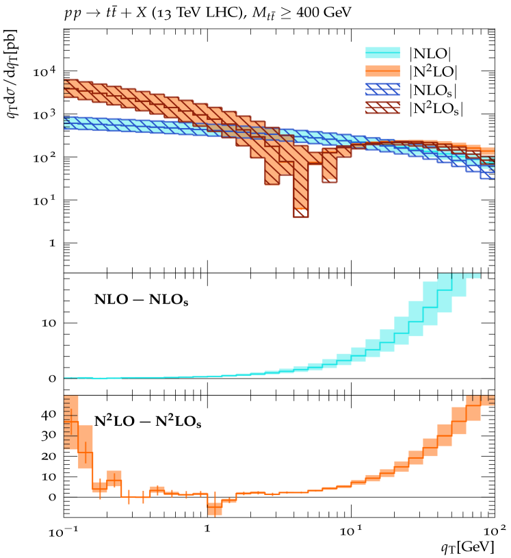
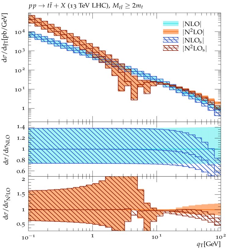
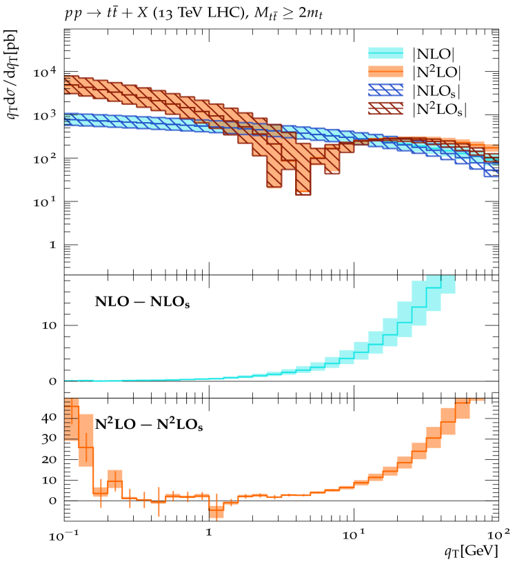
We begin our analysis with an examination of the transverse momentum spectra of the -pair in Fig. 1, where the differential distributions of the SCETHQET approximation are compared to those derived in full QCD. Therein, using cyan and apricot, we show the exact fixed-order full QCD results at NLO and N2LO, respectively, while the approximations are illustrated in the blue and red, labeled NLO and N2LO likewise. During their evaluation, we set the renormalisation and factorisation scales to as our central scale choice and use the interval to estimate the theoretical uncertainties. We represent the scale uncertainties using corresponding coloured solid and hatched bands. In computing N2LO results, we invariably encounter zeros in both the full QCD and approximate calculations around , inducing significant Monte-Carlo statistical uncertainties shown via vertical error bars. Please note, that the distributions to the left of the respective zero-crossings are negative and we are therefore showing the absolute values.
From the main plots in Fig. 1, we observe that, up to N2LO, the asymptotic behaviour of the full QCD calculation is well captured by the leading singular contributions derived using SCETHQET in the low domain for all three slices, including the scale variations. As increases, power corrections progressively corrupt the leading singular approximation and enlarge the discrepancies between NLO and NLO, and N2LO and N2LO, respectively, with the deviations becoming appreciable only around . This phenomenon suggests that, up to N2LO, neither the (Coulomb) potential region [183] near the production threshold nor the well-separated regimes incur additional leading singular terms as .
To make a more quantitative assessment of the leading power approximation, the first (second) subplots of Fig. 1 are devoted to the ratio between NLO (N2LO) and NLO (N2LO). We observe that with only percent level deviations up to , the spectra derived through SCETHQET manage to describe the asymptotic behaviour of the full QCD results at both NLO and N2LO precisions. Further increase in increases the deviations between both approaches as higher-power corrections become increasingly important. Nevertheless, for , the leading power approximation can still account for contribution of the exact differential distributions .
In pursuit of further ascertaining the SCETHQET prediction, we investigate the weighted differential distributions in the low regime, which are expected to observe the power series,
| (3.1) |
where is the LO cross section and the are the coefficients at the respective order of the expansion. The numerical results for are presented in Fig. 2. Differing from the findings of Fig. 1, where acute enhancements are showcased in the low region, the asymptotic behaviour in is alleviated as compared to that of by the application of the weighting factor . To examine whether the leading power behaviour can be entirely replicated by Eq. (2.15), we exhibit the difference between the full QCD results and the EFT ones in the first and second subgraphs of Fig. 2. At NLO, their difference declines monotonously as decreases in all three intervals, demonstrating that the leading power contributions are indeed subtracted by the fixed-order expansion of Eq. (2.15). Regarding the interval GeV, analogous scenarios can also be found at N2LO from the bottom subgraphs in Fig. 2, thereby justifying the EFT results from Eq. (2.15). However, further decreasing incurs non-negligible Monte-Carlo statistical uncertainties, giving rise to deviations between the exact and approximate calculations of up to times the variance estimated there, but still within (sub)percent level relative accuracy w.r.t. the magnitude of .
Finally, we exhibit the and weighted distributions in Fig. 3, evaluated over the full phase space. Unsurprisingly, the behaviours observed in Fig. 3(a) and Fig. 3(b) closely resemble those found in Fig. 1(c) and Fig. 2(c), respectively, as the slice accounts for the bulk of contributions in the phase space integrals. With these findings, we are now in a position to determine the coefficients and comprised in the arguments of the transition function of Eq. (2.62) governing our matching procedure. From the analysis above, we find that for all three invariant-mass slices, the leading power approximation of Eq. (2.15) is capable of reproducing the asymptotic behaviour of the exact QCD calculation up to GeV within percent level accuracy. At a level of of the full theory, this holds until . In light of this, we will make use of
| (3.2) |
as our default choice during the implementation of the matching procedure. With these parameters, the resummation in Eq. (2.15) is fully retained until , after which the transition function phases out the resummation gradually, reducing it to half its size at and completely terminating it at . In order to estimate the theoretical uncertainties associated with our matching procedure, we adopt the following alternative matching parameters
| (3.3) |
and construct an envelope of the calculated spectra.
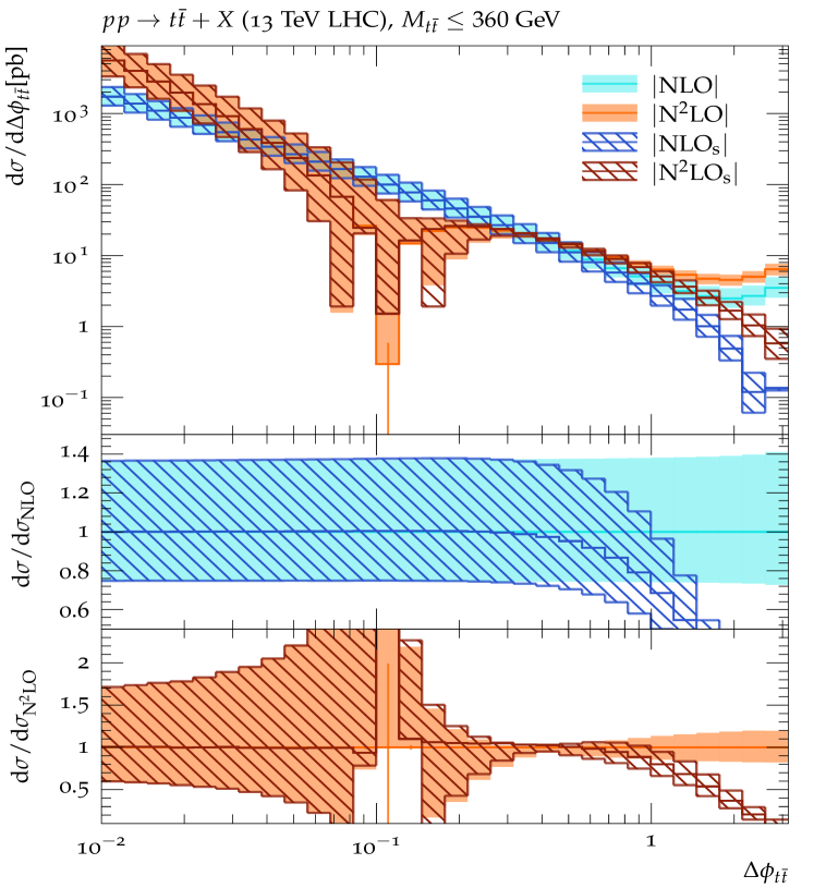
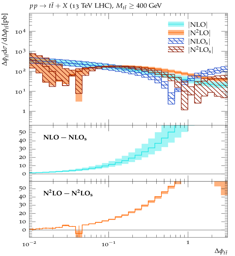
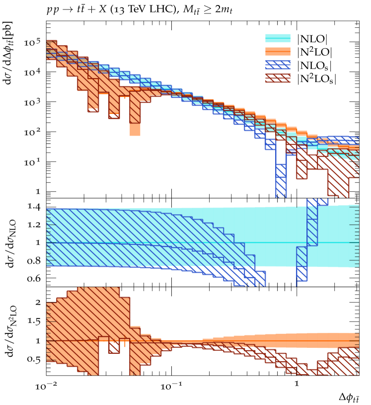
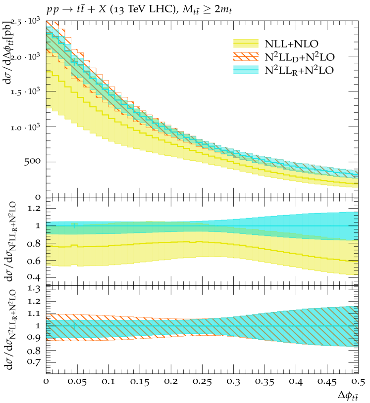
We now move on to the fixed-order results for the spectra of the azimuthal separation of the top and anti-top, , displayed in Fig. 4.555 It should be noted that the results in Figs. 4(c) and 5(c), illustrating the region have already been evaluated in [110]. To facilitate the comparison and later discussion, however, we exhibit them here once again.
Akin to the spectra in Fig. 1, the in the main plots of Fig. 4 exhibit a similarly singular behaviour in the low domain, at both NLO and N2LO. However, comparing the exact and approximate results, even though the SCETHQET calculations are able to reproduce the correct asymptotic behaviour in the region in all three slices, the size of the missing power corrections are markedly larger than in the case. To be precise, at NLO, while the SCETHQET approximation agrees with the full QCD result within percent level accuracy below in the spectra in all three regions of Fig. 1, the distributions of Fig. 4 show a deviation of the EFT-based approximation from the full theory of a few permille around in the slice, increasing to approximately in , and reaching more than in the interval . An analogous behaviour can be found in the N2LO results, although the region where the approximate results deviate from the exact one is shifted to slightly higher , around . To interpret this phenomenon, it merits reminding that the derivation of Eq. (2.15) is subject to an asymptotic expansion of the differential cross section in a given kinematic parameter, for instance, in the spectra and in the ones, where represents a hard scale of the similar magnitude to and . In Fig. 1, focusing on a constant value of , varies gently as changes when progressing through our three slices since the PDFs effectively suppress contributions from, individually, highly boosted top and antitop quarks. However, the situation for in Fig. 4 is different as is sensitive to the variable , the transverse momentum of the top quark measured in the rest frame of the system, and is therefore proportional to in the threshold domain. In turn, scales with in the left panel, and thus takes the typical values of around for , rising to values of about for , and ultimately reaching for . As a consequence of this additional kinematic suppression upon the expansion parameter , weaker power corrections are observed in Fig. 4(a) than in Fig. 4(b), with the largest power corrections found in Fig. 4(c), for constant .
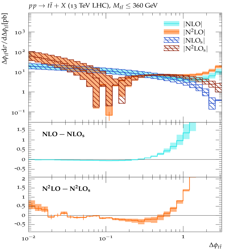
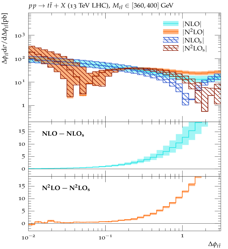
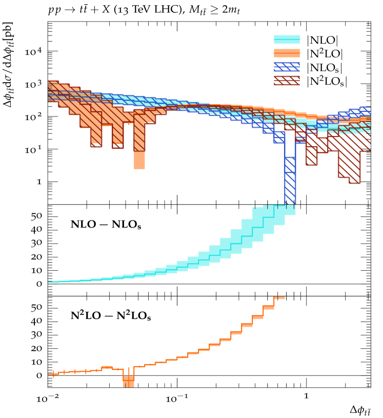
As before, we further assess the quality of the leading power approximation by studying the weighted differential distributions . They are expected to observe the following power series in the asymptotic domain,
| (3.4) | ||||
wherein again is the LO cross section and the are the coefficients at the respective order of the expansion. Numerical results for in our three slices are displayed in Fig. 5. From the main plots therein, we find in all three regions that the approximate SCETHQET calculation can reproduce the desired singular behaviour also of the weighted spectra of the full QCD calculations at both NLO and N2LO. Similarly, as illustrated in the middle and bottom subplots of Fig. 5, their difference progressively decreases as decreases from , until in the non-negligible integration uncertainties are encountered. These observations demonstrate that at least up to N2LO, the fixed-order expansion of Eq. (2.15) is able to describe the leading singular contributions of the full theory.
Again, in a parallel to our appraisal of the approximate spectra, we examine the inclusive and weighted spectra in Fig. 6. Once again, they effectively reproduce the results for as this region carries the bulk of the cross section. With its help we can now determine the coefficients and for the transition function of Eq. (2.62), employed to match the resummed spectrum to its fixed-order counter-part. Considering that the size of the power corrections in the distribution is -dependent, the values of and are chosen differently for each region, i.e.,
| (3.5) |
Therein, in view of the excellent agreement between the approximate and exact results in Fig. 4(a), we extend the active range of the soft and collinear resummation in the region . In consequence, here, the resummation is fully active for and then will be gradually turned off, being reduced to half its strength at and eliminated at . Otherwise, a tightened choice of and is made for both other invariant mass domains. Here, the resummation is restricted to the region , reduced to half-value at , and terminated for . To investigate the sensitivity of the final matched results to the choice of , we also embed the following alternatives as matching parameters,
| (3.6) |
3.3 Resummation-improved and distributions
In the following, we introduce the resummation-improved and spectra based on Eq. (2.15), including the extrapolation into the region using, alternatively, Eq. (2.47) (D-scheme) and Eq. (2.60) (R-scheme). As illustrated in Eqs. (2.7-2.8), our R(a)GE-based resummation is subject to two sets of auxiliary scales, and , characterising the typical scales in the virtuality and rapidity renormalisation, respectively. In addition, the matching procedure of Eq. (2.62), introduces the fixed-order scale . Their default choices are presented in Eq. (2.17) and Eq. (2.64). To estimate the corresponding theoretical uncertainties, we vary all such scales within the intervals and . We denote the resulting variation as . Furthermore, our matching procedure of Eq. (2.62) also introduces the coefficients (for ) and (for ) governing the active range of the soft and beam-collinear resummation. Similarly, while the D-scheme does not introduce further parameters, the R-scheme involves a second matching, see Eq. (2.55), as it embeds terms to mitigate the threshold singularity in the resummation kernel. Its associated parameters parameters are . Their default choice has been presented in Eqs. (3.2), (3.5), and (2.58), respectively. We estimate the uncertainty of the corresponding matching procedure using alternative matching parameter as defined in Eqs. (3.3), (3.6), and (2.59), giving the combined matching uncertainty estimate . Finally, both sources of uncertainties, and , are combined in quadrature, giving the total uncertainty,
| (3.7) |
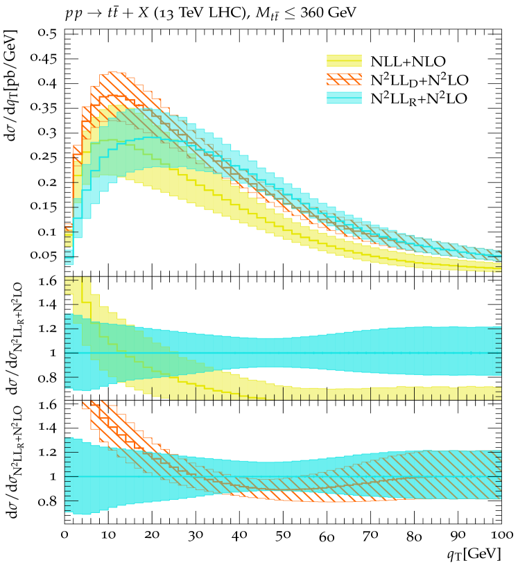
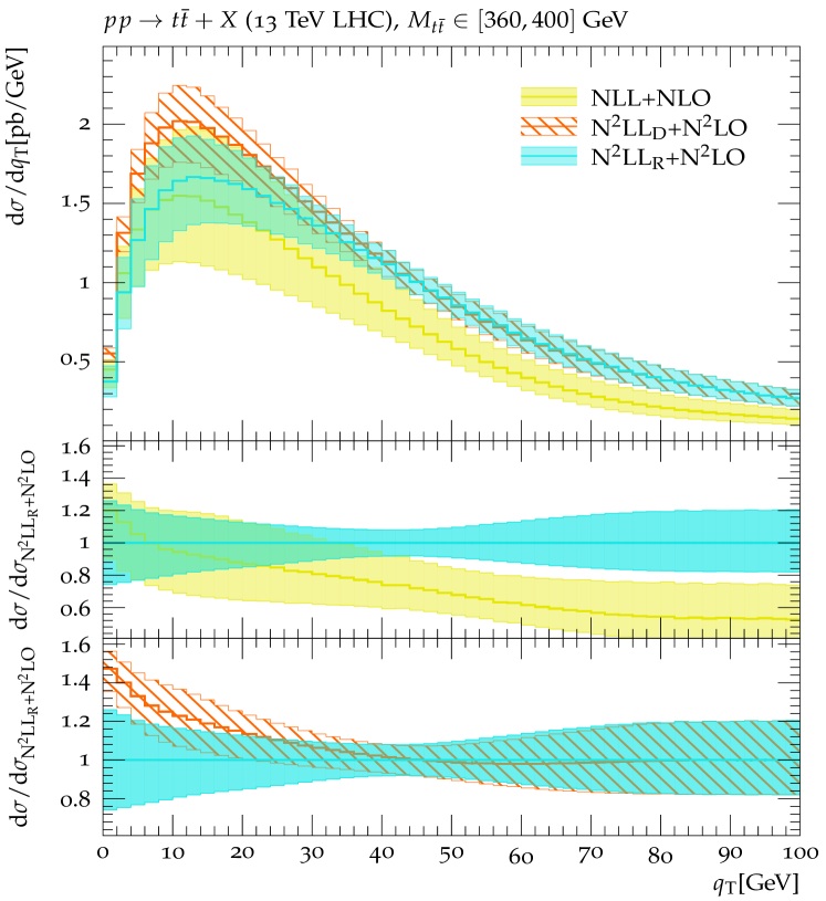
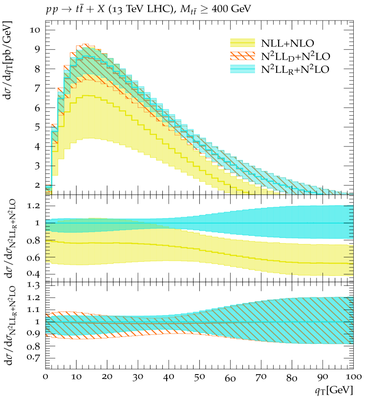
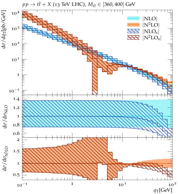
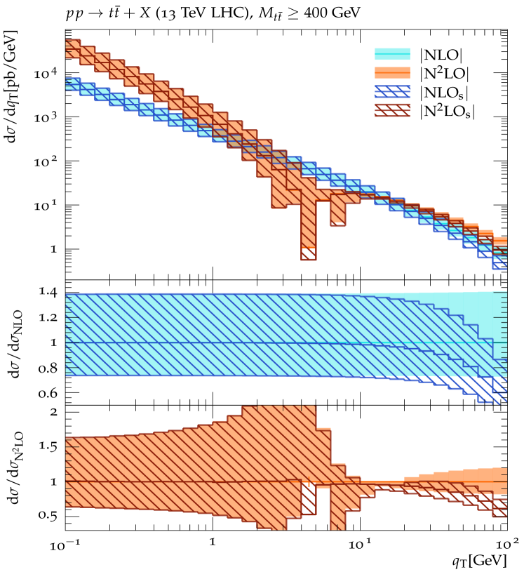
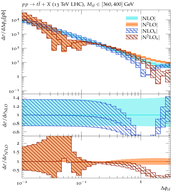
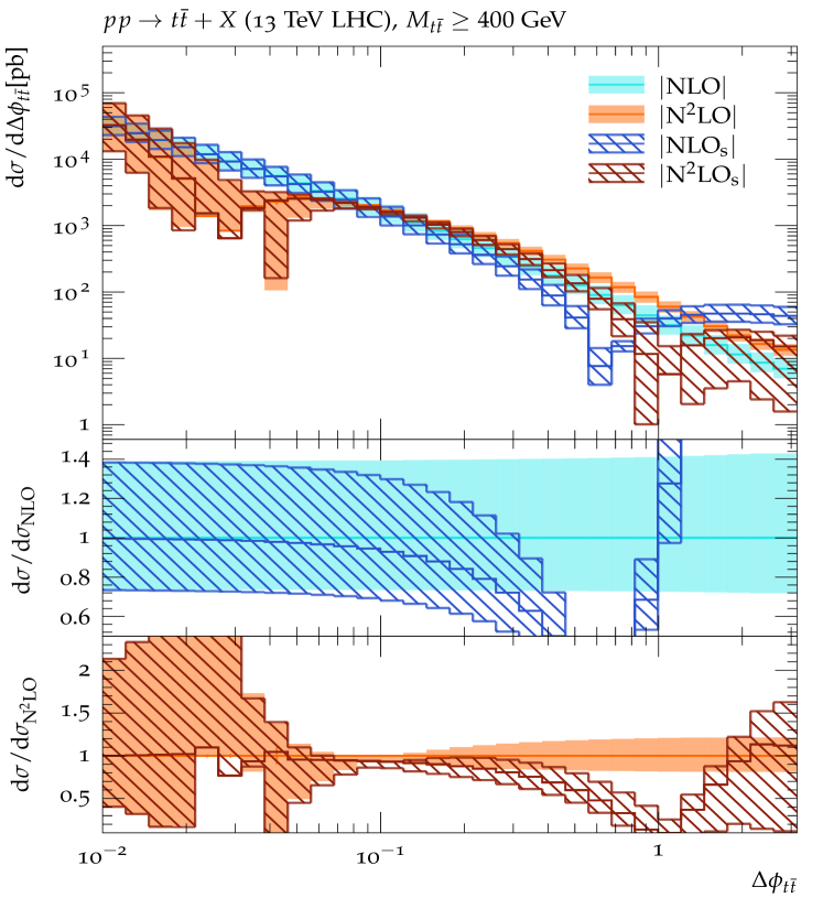
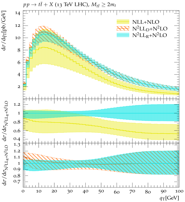
Fig. 7 and 8 display the resummation-improved and differential distributions in the slices , , and . Therein, we display our results at NLL+NLO, N2LLD+N2LO, and N2LLR+N2LO accuracy. The NLL+NLO results are calculated from a literal implementation of Eq. (2.15) since neither the NLL non-cusp evolution kernel nor the tree-level hard functions induce any singular behaviour in the limit , see Eq. (2.38) and Eq. (2.26), and thus no modification of the resummation is required in the threshold regime. Starting from N2LL, however, both the evolution kernels and hard functions introduce threshold divergences in the vicinity of , see Eq. (2.39) and Eq. (2.26), driven by the exchange of Coulomb gluons. To this end, two radically different prescriptions have been proposed in Sec. 2.3 that modify the resummation as in the resummation of the respective observable. The D-scheme was formulated in Eq. (2.47) and shifts the emerging Coulomb singularities to higher logarithmic order, whereas the R-scheme of Eq. (2.60) re-exponentiates such corrections and embeds them in the N2LL evolution kernel. The results derived by both methods are displayed as N2LLD+N2LO and N2LLR+N2LO, respectively.
Examining the spectra displayed in Fig. 7, we observe that the differential cross sections at either large or large increase going from NLL+NLO to N2LL+N2LO, in either scheme, in line with the dominating effects from higher-order corrections (both to the resummation and the fixed-order computation) in these regions. The magnitude of this increase, however, is strongly non-uniform, and ranges from a few percent up to a factor of two. Conversely, at small and small there also exist regions where the cross section in fact decreases as a result of a shift of the Sudakov peak towards higher values when the resummation accuracy is increased, at least in the R-scheme. Generally, the uncertainties of the calculation are reduced when including the next order in the perturbative expansion, both in terms of the coupling parameter and the resummed large logarithms. Unsurprisingly though, the increased convergence is spoiled in the threshold regime as and vanish simultaneously.
Among the N2LL+N2LO results, the central values of N2LLD+N2LO and N2LLR+N2LO nearly coincide throughout the whole range for , as do their uncertainties, with small differences being visible in the resummation region. When moving to smaller invariant masses, however, differences between both schemes develop in the low region, culminating as or . To interpret this phenomenon, we recall that D- and R-scheme employ distinct methods to organise the perturbative corrections. More explicitly, the D-scheme, see Eq. (2.47), shifts the non-logarithmic components of the product of the evolution kernel and the fixed-order functions to N3LL and beyond (and therefore does not include them at N2LLD+N2LO), whereas the R-scheme, see Eq. (2.60), in part re-exponentiates them in a dedicated Sudakov factor. In the absence of any asymptotic behavior in , the difference between the N2LLD+N2LO and N2LLR+N2LO results is of N3LL order and beyond. Hence, we expect it to leave only small residual effects for . Lowering towards the threshold regime, however, non-logarithmic contributions in can develop power-like divergences in , see Eqs. (2.26) and Eq. (2.39), introducing non-negligible corrections (in ). This, in turn, induces an increasing divergence between both schemes, rendering their difference in the resummation region as large as that to the formally lower-order NLL+NLO computation.
Analogous reasoning can also be employed to analyse the uncertainty bands in Fig. 7. For instance, in the low domain of the region, N2LLR+N2LO presents the smallest uncertainty due to the inclusion of higher-order perturbative contributions partially compensating scale variations in the Sudakov kernels. It is well contained by N2LLD+N2LO band and marginally overlaps with the NLL+NLO one. This observation demonstrates the perturbative convergences in the soft and beam-collinear resummation in this regime. Our findings change, though, as we move towards smaller or , towards the threshold region. Here, a distinct pattern can be found both in Fig. 7(a) and Fig. 7(b) where formally non-logarithmic products of the resummation kernel and the hard function that are removed in the D-scheme but included in the R-scheme can no longer be ignored. To be precise, focussing on the asymptotic domain of Fig. 7(a) and Fig. 7(b), we find that even though the uncertainty bands of N2LLD+N2LO and N2LLR+N2LO still overlap with those of the NLL+NLO computation, significant deviations manifest themselves in the limit outside their respective uncertainties. This observation indicates that the perturbative truncation in line with the logarithmic counting laws of the soft and beam-collinear resummation invokes substantial higher order corrections in the domain . Therefore, to deliver precise predictions in this region, a more systematic re-collection of the threshold enhancements together with the soft and beam-collinear radiation is still needed.
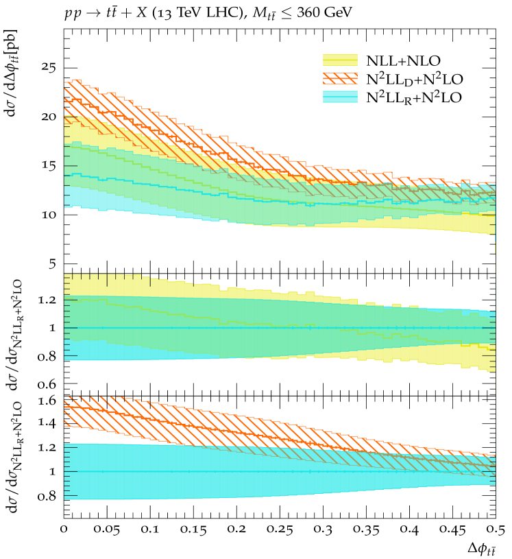
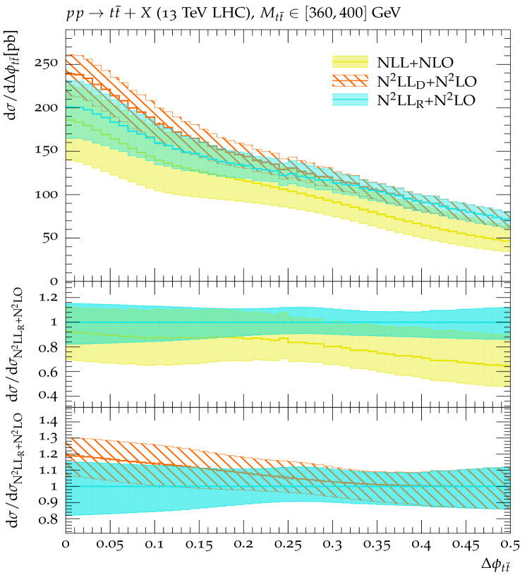
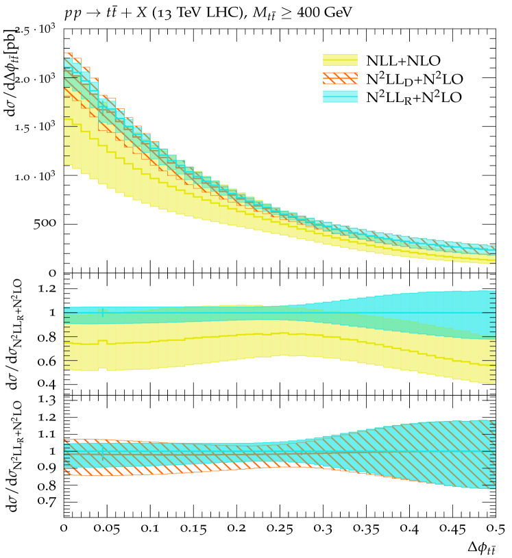
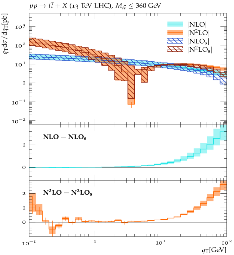
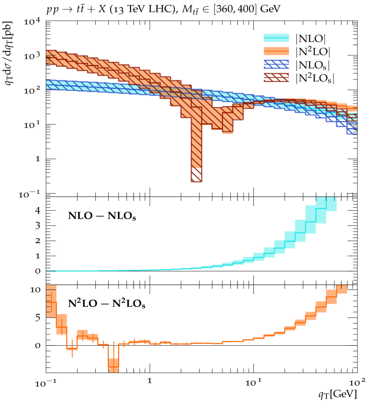
The resummation-improved distributions are shown in Fig. 8 in the three invariant mass slices , , and . Again, the NLL+NLO result in the slice has already been published in [110], which is showcased here for comparison purposes. We observe that, at variance with the spectra of Fig. 7 where Sudakov peaks are formed in the asymptotic domain, the spectra grow monotonically as . To understand this structural difference, we remind the reader that while both the and resummations comprise the same partonic kernels in Eqs. (2.7-2.8), as well as modifications in the D- and R-scheme, see Eq. (2.47) and Eq. (2.60), which approach constants as and vanish, the calculation of the spectra, see Eq. (2.15), invokes an additional kinematic suppression in the spectrum which is absent in the case. In consequence, the spectrum develops a Sudakov peak in the vicinity of , whereas the spectrum does not. Furthermore, in Fig. 8 we again compare our results at NLL+NLO and N2LL+N2LO accuracy, the latter again both in the D- and the R-scheme. Akin to the scenario in Fig. 7, we also observe perturbative convergence of the resummation in the interval with the increase in the logarithmic accuracy. Reducing , as before, leads to a gradual corruption through the threshold singular terms as . This echoes the necessity to re-collect the threshold enhancements during the soft and beam-collinear resummation for this spectrum as well, especially when the domain and is of concern.
Ultimately, we present in Fig. 9 the single differential distributions and over the whole phase space, integrated over all values. Therein, the results at NLL+NLO in Fig. 9(a) () and 9(b) () are comparable to those of Fig. 7(c) and 8(c), respectively, in both shape and magnitude, owing to the fact that the interval accounts for the bulk of the cross section. At N2LL+N2LO accuracy, however, whilst the distribution still mostly resembles the one in Fig. 8(c), including the convergence of both the central value and the uncertainty estimates of the N2LLD+N2LO and N2LLR+N2LO calculations in the asymptotic domain, the spectrum exhibits a sensitivity of around to the extrapolation scheme as , differing from Fig. 7(c). To interpret this, it merits recalling that the threshold limit imposes stronger kinematical restriction on than on , where the former experiences an additional kinematic factor of while there is no such suppression factor for the latter, see Eqs. (2.15). As a result, during the phase space integration, the contributions from the threshold region contribute very little to , but still have an appreciable impact in low regime of . At last, it is paramount to emphasise that in spite of the numerical insensitivity of the distribution to the extrapolation prescriptions, implementing the literal resummation of Eq. (2.15) onto is still impossible without taking care of the divergences in emerging at N2LL. Otherwise, threshold singularities would develop in the limit and in turn leading to a divergent phase space integration, as elucidated in Eqs. (2.44).
4 Conclusions
In this paper we presented the resummation-improved transverse momentum and, for the first time, azimuthal separation spectra of the -pair at N2LL+N2LO accuracy. In order to include the entire top-antitop production phase space, ranging from very high invariant -pair masses, , down to the production threshold region at (), we isolated the arising threshold singularities at that order and incorporated them into our resummation formalism. To address the inherent ambiguities of such a procedure, we formulated to fundamentally different schemes. While the D-scheme simply shifts the poles in to a higher logarithmic accuracy which is not included here, the novel R-scheme re-collects such contributions in part and includes them in the soft-collinear Sudakov form factor. Their difference is formally of N3LL and can be used to estimate the theoretical uncertainty of the treatment of the Coulomb singularity.
In order to analyse the properties and numerical predictions of our formalism, we investigated the double differential distributions and . We found that at large top-pair invariant masses both the D- and R-scheme give consistent results, agreeing with our expectation that the -dependent non-logarithmic corrections are unimportant in this region. Conversely, approaching the threshold region the differences between both schemes become apparent. While the D-scheme predicts only slight alterations of the NLL Sudakov peak in the spectrum, the R-scheme shifts the Sudakov peak to somewhat larger at very small . Similar results are found for the spectra. Despite the absence of a Sudakov peak structure, the differences between both schemes manifest themselves in lower predicted cross sections in the R-scheme as both and approach zero.
Finally, we integrated all invariant mass regions to arrive at predictions for the single-differential and distributions. Their features follow mostly the results calculated far away from the threshold region, by virtue of their dominance in the integrated cross section, and show only mild differences between the D- and R-scheme. It is noteworthy though, that the spectrum experiences an additional phase space suppression in the threshold limit such that the Coulomb-gluon affected region plays a smaller role in the inclusive spectrum than it does for . Consequently, we found much smaller differences between both extrapolation schemes in . This suggests that, in comparison to the case, the inclusive spectrum is better suited to a pure soft-collinear resummation, at least up to N2LL+N2LO precision. In bears no mention, though, that singularities are present within this integration over the whole invariant mass range at N2LL+N2LO order, and a naïve soft-collinear resummation is not possible without addressing them. Despite their radical differences, the fact that the predictions of the D- and R-scheme largely coincide shows the power of our formalism.
Ultimately, only a rigorous simultaneous resummation of both soft-collinear and Coulomb divergences will remove this scheme dependence and yield reliable predictions throughout the entire range. We will, however, leave such developments for future work.
Acknowledgements
WJ would like to thank Li Lin Yang for sharing valuable details in computing the hard evolution kernel in [104, 105, 88, 284]. WJ is also grateful to Guoxing Wang for the helpful discussion on the threshold soft function in [239]. WJ and MS would also like to express our gratitude to Ben Pecjak for taking the time to respond to our numerous queries. MS is funded by the Royal Society through a University Research Fellowship (URF\R1\180549, URF\R\231031) and an Enhancement Award (RGF\EA\181033, CEC19\100349, and RF\ERE\210397) as well as the STFC (ST/X003167/1 and ST/X000745/1).
Appendix A Numerical results of hard-scale evolution kernel
In this appendix we deliver a numerical comparison amongst the original non-cusp evolution kernel in Eqs. (2.12-2.13) as proposed in [169, 170], the leading singular approximation from Eqs. (2.38-2.39), and the expansion of the re-exponentiated kernel in Eq. (2.56). During our computation, we fix and as well as the scattering angle of the top quark .
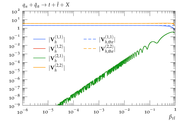
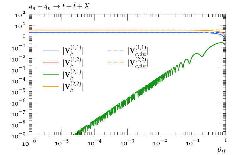
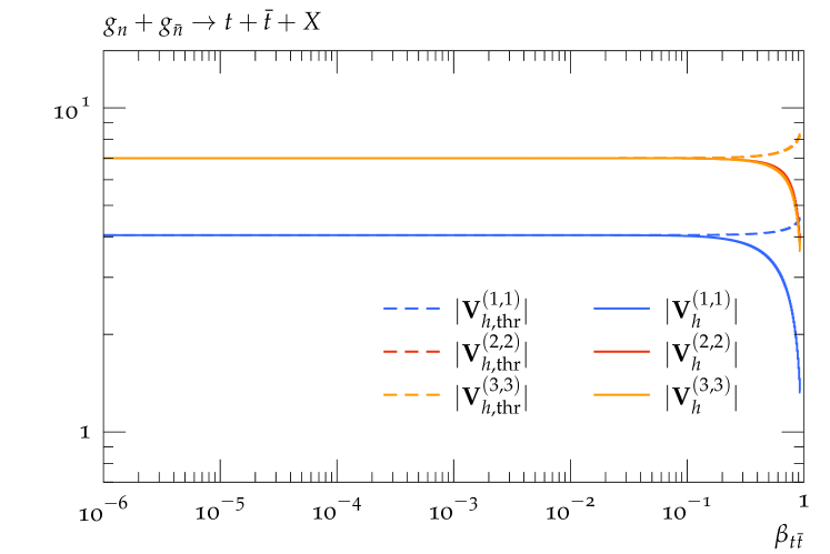
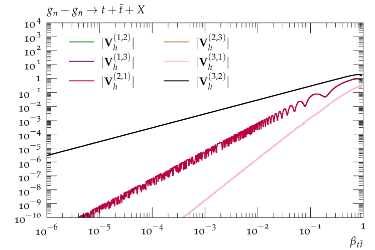
Fig. 10 exhibits the NLL results of in Eq. (2.12) and in Eq. (2.38) in solid and dashed lines, respectively. Therein, the dependence of all the entries of is displayed with respect to . For , we show the non-zero components only. Due to the facts that the leading threshold enhanced terms in the NLO anomalous dimension only manifest themselves in the imaginary parts and that the complete Coulomb singular behaviour has been exponentiated at NLL in both Eq. (2.12) and Eq. (2.38), the NLL kernel illustrated in Fig. 10 invokes no divergence as . Comparing with , we find that the leading approximation is capable of replicating the correct asymptotic behaviour of all the diagonal entries of , while the non-diagonal elements of become progressive smaller in the low region. This indicates the non-diagonal entries of are all power suppressed in magnitude and it is thus in agreement with the absence of the off-diagonal contributions in in Eq. (2.38).
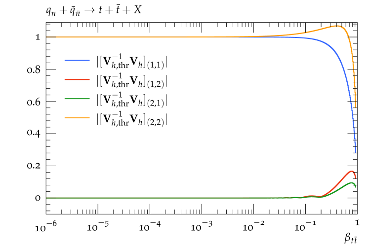
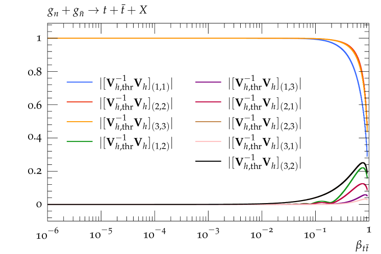
In a bid to scrutinise our leading approximation in Eq. (2.38) further, we plot the result of the product in Fig. 11. We observe that approaches the unity matrix for all three partonic processes of interest. This phenomenon shows that is able to serve as a qualified inverse matrix of in the vicinity of . Further, it details that the approximation in Eq. (2.38) indeed manages to reproduce the leading asymptotic behaviour of Eq. (2.12).
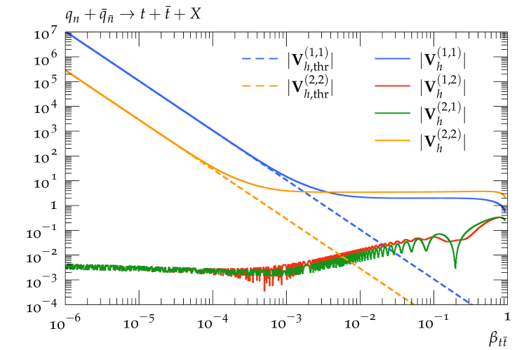
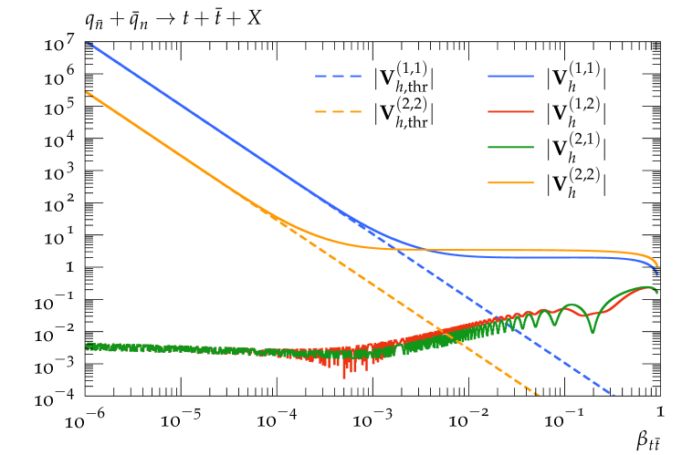
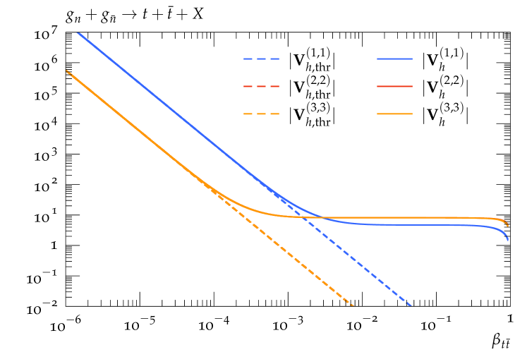

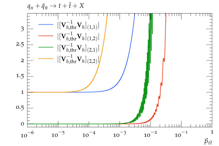
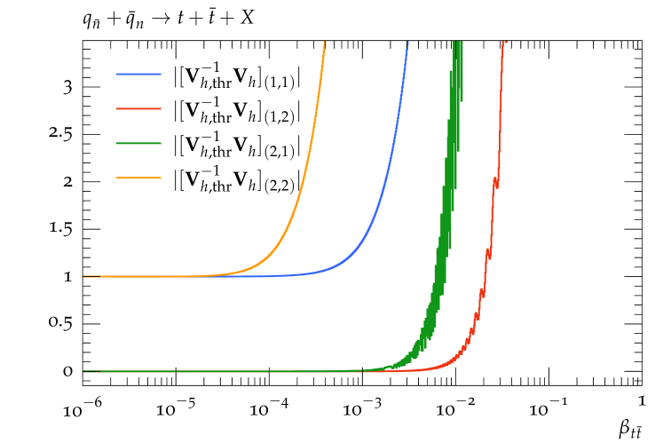
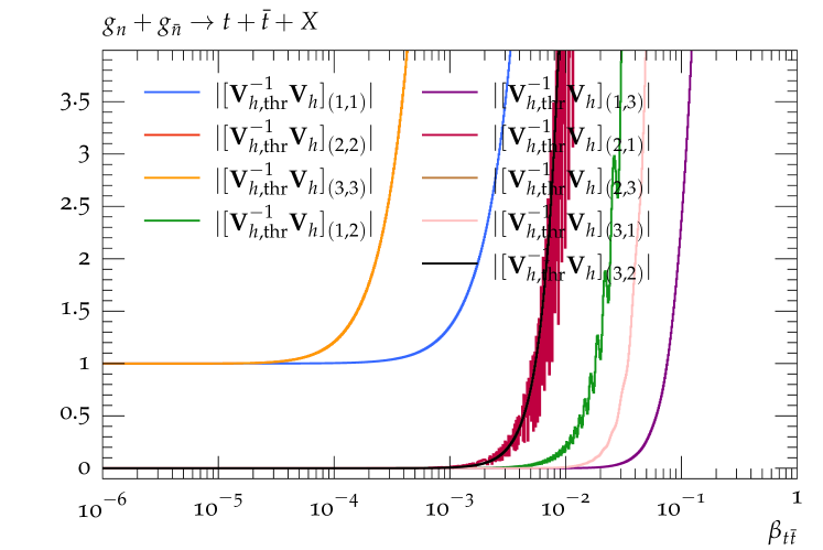
In Figs. 12 we confront of Eq. (2.13) with of Eq. (2.39) at N2LL. At variance with the findings of Figs. 10 and 11, the diagonal entries of develop divergent behaviour in the threshold domain, as a result of the Coulomb singularity residing in Eq. (2.35), which is able to replicate at N2LL. Further, differing from at NLL, where all the non-diagonal entries in Fig. 10 generally decline in magnitude as reduces, the non-diagonal constituents in Fig. 12 can experience enhancements in the threshold domain, such as in Fig. 12(d). The reason for this phenomenon is that in the expression of Eq. (2.39), only the leading singular terms of Eq. (2.39), which are of , have been taken into account. Divergence of are, however, still possible. To verify that there is no stronger divergent behaviour in non-diagonal elements other than that of Eq. (2.39), we present the results of in Fig. 13. It is found that all but the diagonal elements are reduced substantially as , while all the diagonal elements of the product approach unity. This unambiguously shows that our leading approximation in Eq. (2.39) can describe the asymptotic behaviour of Eq. (2.13) at N2LL as well.
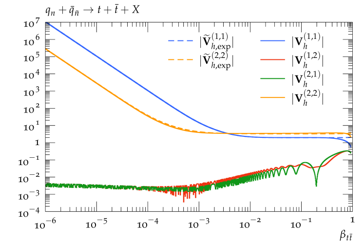
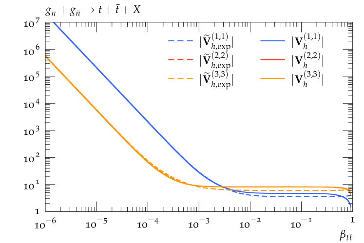
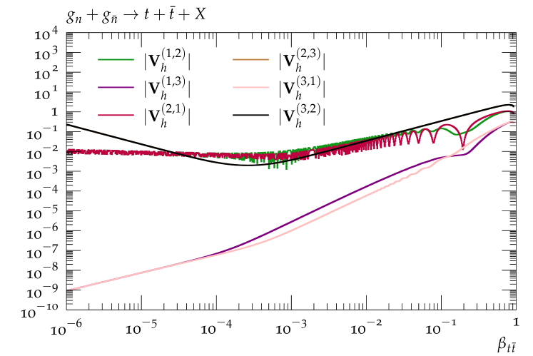
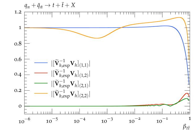
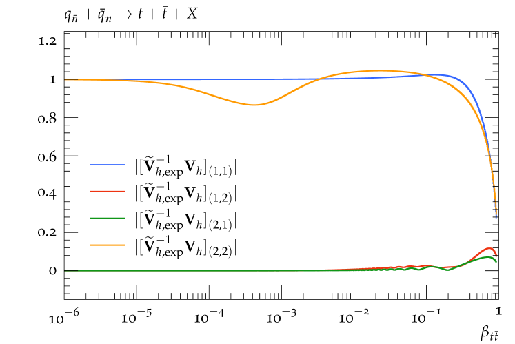
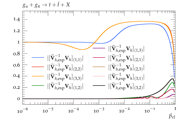
Eventually, Figs. 14 and 15 depict the results of of Eq. (2.13) and in Eq. (2.56) at N2LL, the expansion of the re-exponentiated Sudakov factor. Owing to the fact that in comparison with the leading singular result of in Eq. (2.39), is embedded with more power corrections, the agreement between and is considerably improved compared to Figs. 12 and 13. For instance, focussing on the quark-induced process, while in Fig. 13(a), the deviation between the leading approximation in Eq. (2.39) and in Eq. (2.13) rapidly surges above , in Fig. 15(a), numerical agreement of and holds up to within around . In light of this excellent agreement, in matching the re-exponentiated Sudakov factor onto in Eq. (2.55), we choose the matching parameters and as defined in Eq. (2.58). In this way, the re-exponentiation impact is fully switched on in the domain but then gets gradually faded out until the total shutdown at . This choice of this active range brings the difference between and under control, i.e. generally below for all three partonic channels, and also steers clear of the tail region in Fig. 15 where the power correction to the small expansion escalates dramatically.
References
- [1] G. Aad et al., ATLAS collaboration, Measurement of the production cross-section in pp collisions at = 5.02 TeV with the ATLAS detector, JHEP 06 (2023), 138, [arXiv:2207.01354 [hep-ex]].
- [2] A. M. Sirunyan et al., CMS collaboration, Measurement of the inclusive cross section in pp collisions at TeV using final states with at least one charged lepton, JHEP 03 (2018), 115, [arXiv:1711.03143 [hep-ex]].
- [3] ATLAS collaboration, Measurement of the production cross-section using dilepton events in collisions at TeV with the ATLAS detector.
- [4] A. Tumasyan et al., CMS collaboration, Measurement of the inclusive production cross section in proton-proton collisions at = 5.02 TeV, JHEP 04 (2022), 144, [arXiv:2112.09114 [hep-ex]].
- [5] S. Chatrchyan et al., CMS collaboration, Measurement of the Production Cross Section in the All-Jet Final State in pp Collisions at = 7 TeV, JHEP 05 (2013), 065, [arXiv:1302.0508 [hep-ex]].
- [6] G. Aad et al., ATLAS collaboration, Measurement of the production cross-section using events with b-tagged jets in pp collisions at = 7 and 8 with the ATLAS detector, Eur. Phys. J. C 74 (2014), no. 10, 3109, [arXiv:1406.5375 [hep-ex]], [Addendum: Eur.Phys.J.C 76, 642 (2016)].
- [7] G. Aad et al., ATLAS collaboration, Measurement of the top quark pair production cross-section with ATLAS in the single lepton channel, Phys. Lett. B 711 (2012), 244–263, [arXiv:1201.1889 [hep-ex]].
- [8] V. Khachatryan et al., CMS collaboration, Measurement of the t-tbar production cross section in the e-mu channel in proton-proton collisions at sqrt(s) = 7 and 8 TeV, JHEP 08 (2016), 029, [arXiv:1603.02303 [hep-ex]].
- [9] V. Khachatryan et al., CMS collaboration, Measurements of the production cross section in lepton+jets final states in pp collisions at 8 TeV and ratio of 8 to 7 TeV cross sections, Eur. Phys. J. C 77 (2017), no. 1, 15, [arXiv:1602.09024 [hep-ex]].
- [10] S. Chatrchyan et al., CMS collaboration, Measurement of the Production Cross Section in Collisions at TeV with Lepton + Jets Final States, Phys. Lett. B 720 (2013), 83–104, [arXiv:1212.6682 [hep-ex]].
- [11] R. Aaij et al., LHCb collaboration, First observation of top quark production in the forward region, Phys. Rev. Lett. 115 (2015), no. 11, 112001, [arXiv:1506.00903 [hep-ex]].
- [12] G. Aad et al., ATLAS, CMS collaboration, Combination of inclusive top-quark pair production cross-section measurements using ATLAS and CMS data at = 7 and 8 TeV, JHEP 07 (2023), 213, [arXiv:2205.13830 [hep-ex]].
- [13] G. Aad et al., ATLAS collaboration, Measurement of the top-quark mass in -jet events collected with the ATLAS detector in collisions at TeV, JHEP 11 (2019), 150, [arXiv:1905.02302 [hep-ex]].
- [14] M. Aaboud et al., ATLAS collaboration, Measurement of top quark pair differential cross-sections in the dilepton channel in collisions at = 7 and 8 TeV with ATLAS, Phys. Rev. D 94 (2016), no. 9, 092003, [arXiv:1607.07281 [hep-ex]], [Addendum: Phys.Rev.D 101, 119901 (2020)].
- [15] V. Khachatryan et al., CMS collaboration, Measurement of the integrated and differential production cross sections for high- top quarks in collisions at 8 TeV, Phys. Rev. D 94 (2016), no. 7, 072002, [arXiv:1605.00116 [hep-ex]].
- [16] V. Khachatryan et al., CMS collaboration, Measurement of the production cross section in the all-jets final state in pp collisions at TeV, Eur. Phys. J. C 76 (2016), no. 3, 128, [arXiv:1509.06076 [hep-ex]].
- [17] G. Aad et al., ATLAS collaboration, Inclusive and differential cross-sections for dilepton production measured in = 13 TeV pp collisions with the ATLAS detector, JHEP 07 (2023), 141, [arXiv:2303.15340 [hep-ex]].
- [18] V. Khachatryan et al., CMS collaboration, Measurement of the top quark pair production cross section in proton-proton collisions at 13 TeV, Phys. Rev. Lett. 116 (2016), no. 5, 052002, [arXiv:1510.05302 [hep-ex]].
- [19] R. Aaij et al., LHCb collaboration, Measurement of forward top pair production in the dilepton channel in collisions at TeV, JHEP 08 (2018), 174, [arXiv:1803.05188 [hep-ex]].
- [20] M. Aaboud et al., ATLAS collaboration, Measurement of jet activity produced in top-quark events with an electron, a muon and two -tagged jets in the final state in collisions at TeV with the ATLAS detector, Eur. Phys. J. C 77 (2017), no. 4, 220, [arXiv:1610.09978 [hep-ex]].
- [21] G. Aad et al., ATLAS collaboration, Measurement of the production cross-section and lepton differential distributions in dilepton events from collisions at with the ATLAS detector, Eur. Phys. J. C 80 (2020), no. 6, 528, [arXiv:1910.08819 [hep-ex]].
- [22] G. Aad et al., ATLAS collaboration, Measurement of the production cross-section in the lepton+jets channel at TeV with the ATLAS experiment, Phys. Lett. B 810 (2020), 135797, [arXiv:2006.13076 [hep-ex]].
- [23] A. M. Sirunyan et al., CMS collaboration, Measurement of the top quark pair production cross section in dilepton final states containing one lepton in pp collisions at 13 TeV, JHEP 02 (2020), 191, [arXiv:1911.13204 [hep-ex]].
- [24] CMS collaboration, Measurement of the production cross section at 13 TeV in the all-jets final state.
- [25] A. M. Sirunyan et al., CMS collaboration, Measurement of the production cross section, the top quark mass, and the strong coupling constant using dilepton events in pp collisions at 13 TeV, Eur. Phys. J. C 79 (2019), no. 5, 368, [arXiv:1812.10505 [hep-ex]].
- [26] CMS collaboration, First measurement of the top quark pair production cross section in proton-proton collisions at .
- [27] G. Aad et al., ATLAS collaboration, Measurement of the tt¯ cross section and its ratio to the Z production cross section using pp collisions at s=13.6 TeV with the ATLAS detector, Phys. Lett. B 848 (2024), 138376, [arXiv:2308.09529 [hep-ex]].
- [28] G. Aad et al., ATLAS collaboration, Measurements of top quark pair relative differential cross-sections with ATLAS in collisions at TeV, Eur. Phys. J. C 73 (2013), no. 1, 2261, [arXiv:1207.5644 [hep-ex]].
- [29] S. Chatrchyan et al., CMS collaboration, Measurement of Differential Top-Quark Pair Production Cross Sections in collisions at TeV, Eur. Phys. J. C 73 (2013), no. 3, 2339, [arXiv:1211.2220 [hep-ex]].
- [30] G. Aad et al., ATLAS collaboration, Measurements of normalized differential cross sections for production in pp collisions at TeV using the ATLAS detector, Phys. Rev. D 90 (2014), no. 7, 072004, [arXiv:1407.0371 [hep-ex]].
- [31] G. Aad et al., ATLAS collaboration, Differential top-antitop cross-section measurements as a function of observables constructed from final-state particles using pp collisions at TeV in the ATLAS detector, JHEP 06 (2015), 100, [arXiv:1502.05923 [hep-ex]].
- [32] A. M. Sirunyan et al., CMS collaboration, Measurement of double-differential cross sections for top quark pair production in pp collisions at TeV and impact on parton distribution functions, Eur. Phys. J. C 77 (2017), no. 7, 459, [arXiv:1703.01630 [hep-ex]].
- [33] V. Khachatryan et al., CMS collaboration, Measurement of the differential cross section for top quark pair production in pp collisions at , Eur. Phys. J. C 75 (2015), no. 11, 542, [arXiv:1505.04480 [hep-ex]].
- [34] G. Aad et al., ATLAS collaboration, Measurements of top-quark pair differential cross-sections in the lepton+jets channel in collisions at TeV using the ATLAS detector, Eur. Phys. J. C 76 (2016), no. 10, 538, [arXiv:1511.04716 [hep-ex]].
- [35] G. Aad et al., ATLAS collaboration, Measurement of the differential cross-section of highly boosted top quarks as a function of their transverse momentum in = 8 TeV proton-proton collisions using the ATLAS detector, Phys. Rev. D 93 (2016), no. 3, 032009, [arXiv:1510.03818 [hep-ex]].
- [36] CMS collaboration, Differential cross section measurements for the production of top quark pairs and of additional jets using dilepton events from pp collisions at = 13 TeV, arXiv:2402.08486 [hep-ex].
- [37] CMS collaboration, Measurement of differential cross sections for the production of top quark pairs and of additional jets in pp collisions at .
- [38] V. Khachatryan et al., CMS collaboration, Measurement of differential cross sections for top quark pair production using the lepton+jets final state in proton-proton collisions at 13 TeV, Phys. Rev. D 95 (2017), no. 9, 092001, [arXiv:1610.04191 [hep-ex]].
- [39] M. Aaboud et al., ATLAS collaboration, Measurements of top-quark pair differential cross-sections in the channel in collisions at TeV using the ATLAS detector, Eur. Phys. J. C 77 (2017), no. 5, 292, [arXiv:1612.05220 [hep-ex]].
- [40] A. M. Sirunyan et al., CMS collaboration, Measurement of normalized differential cross sections in the dilepton channel from pp collisions at TeV, JHEP 04 (2018), 060, [arXiv:1708.07638 [hep-ex]].
- [41] A. M. Sirunyan et al., CMS collaboration, Measurement of normalised multi-differential cross sections in pp collisions at TeV, and simultaneous determination of the strong coupling strength, top quark pole mass, and parton distribution functions, Eur. Phys. J. C 80 (2020), no. 7, 658, [arXiv:1904.05237 [hep-ex]].
- [42] A. M. Sirunyan et al., CMS collaboration, Measurement of differential production cross sections using top quarks at large transverse momenta in collisions at 13 TeV, Phys. Rev. D 103 (2021), no. 5, 052008, [arXiv:2008.07860 [hep-ex]].
- [43] G. Aad et al., ATLAS collaboration, Measurements of top-quark pair single- and double-differential cross-sections in the all-hadronic channel in collisions at using the ATLAS detector, JHEP 01 (2021), 033, [arXiv:2006.09274 [hep-ex]].
- [44] G. Aad et al., ATLAS collaboration, Measurements of differential cross-sections in top-quark pair events with a high transverse momentum top quark and limits on beyond the Standard Model contributions to top-quark pair production with the ATLAS detector at = 13 TeV, JHEP 06 (2022), 063, [arXiv:2202.12134 [hep-ex]].
- [45] G. Aad et al., ATLAS collaboration, Differential cross-section measurements using boosted top quarks in the all-hadronic final state with 139 fb-1 of ATLAS data, JHEP 04 (2023), 080, [arXiv:2205.02817 [hep-ex]].
- [46] A. Tumasyan et al., CMS collaboration, Measurement of differential production cross sections in the full kinematic range using lepton+jets events from proton-proton collisions at = 13 TeV, Phys. Rev. D 104 (2021), no. 9, 092013, [arXiv:2108.02803 [hep-ex]].
- [47] A. M. Sirunyan et al., CMS collaboration, Measurement of differential cross sections for the production of top quark pairs and of additional jets in lepton+jets events from pp collisions at 13 TeV, Phys. Rev. D 97 (2018), no. 11, 112003, [arXiv:1803.08856 [hep-ex]].
- [48] A. M. Sirunyan et al., CMS collaboration, Measurements of differential cross sections in proton-proton collisions at 13 TeV using events containing two leptons, JHEP 02 (2019), 149, [arXiv:1811.06625 [hep-ex]].
- [49] G. Aad et al., ATLAS collaboration, Measurements of top-quark pair differential and double-differential cross-sections in the +jets channel with collisions at TeV using the ATLAS detector, Eur. Phys. J. C 79 (2019), no. 12, 1028, [arXiv:1908.07305 [hep-ex]], [Erratum: Eur.Phys.J.C 80, 1092 (2020)].
- [50] P. Nason, S. Dawson and R. K. Ellis, The Total Cross-Section for the Production of Heavy Quarks in Hadronic Collisions, Nucl. Phys. B 303 (1988), 607–633.
- [51] W. Beenakker, H. Kuijf, W. L. van Neerven and J. Smith, QCD Corrections to Heavy Quark Production in p anti-p Collisions, Phys. Rev. D 40 (1989), 54–82.
- [52] W. Beenakker, W. L. van Neerven, R. Meng, G. A. Schuler and J. Smith, QCD corrections to heavy quark production in hadron hadron collisions, Nucl. Phys. B 351 (1991), 507–560.
- [53] M. L. Mangano, P. Nason and G. Ridolfi, Heavy quark correlations in hadron collisions at next-to-leading order, Nucl. Phys. B 373 (1992), 295–345.
- [54] M. Czakon, P. Fiedler and A. Mitov, Total Top-Quark Pair-Production Cross Section at Hadron Colliders Through , Phys. Rev. Lett. 110 (2013), 252004, [arXiv:1303.6254 [hep-ph]].
- [55] M. Czakon, D. Heymes and A. Mitov, High-precision differential predictions for top-quark pairs at the LHC, Phys. Rev. Lett. 116 (2016), no. 8, 082003, [arXiv:1511.00549 [hep-ph]].
- [56] M. Czakon, P. Fiedler, D. Heymes and A. Mitov, NNLO QCD predictions for fully-differential top-quark pair production at the Tevatron, JHEP 05 (2016), 034, [arXiv:1601.05375 [hep-ph]].
- [57] M. Czakon, D. Heymes and A. Mitov, fastNLO tables for NNLO top-quark pair differential distributions, arXiv:1704.08551 [hep-ph].
- [58] M. Czakon, D. Heymes, A. Mitov, D. Pagani, I. Tsinikos and M. Zaro, Top-pair production at the LHC through NNLO QCD and NLO EW, JHEP 10 (2017), 186, [arXiv:1705.04105 [hep-ph]].
- [59] S. Catani, S. Devoto, M. Grazzini, S. Kallweit, J. Mazzitelli and H. Sargsyan, Top-quark pair hadroproduction at next-to-next-to-leading order in QCD, Phys. Rev. D 99 (2019), no. 5, 051501, [arXiv:1901.04005 [hep-ph]].
- [60] S. Catani, S. Devoto, M. Grazzini, S. Kallweit and J. Mazzitelli, Top-quark pair hadroproduction at NNLO: differential predictions with the mass, JHEP 08 (2020), no. 08, 027, [arXiv:2005.00557 [hep-ph]].
- [61] M. Czakon, A. Mitov, M. Pellen and R. Poncelet, NNLO QCD predictions for W+c-jet production at the LHC, JHEP 06 (2021), 100, [arXiv:2011.01011 [hep-ph]].
- [62] M. L. Czakon, T. Generet, A. Mitov and R. Poncelet, B-hadron production in NNLO QCD: application to LHC t events with leptonic decays, JHEP 10 (2021), 216, [arXiv:2102.08267 [hep-ph]].
- [63] S. Catani, S. Devoto, M. Grazzini, S. Kallweit and J. Mazzitelli, Top-quark pair production at the LHC: Fully differential QCD predictions at NNLO, JHEP 07 (2019), 100, [arXiv:1906.06535 [hep-ph]].
- [64] M. V. Garzelli, J. Mazzitelli, S. O. Moch and O. Zenaiev, Top-quark pole mass extraction at NNLO accuracy, from total, single- and double-differential cross sections for + X production at the LHC, JHEP 05 (2024), 321, [arXiv:2311.05509 [hep-ph]].
- [65] W. Bernreuther and Z.-G. Si, Distributions and correlations for top quark pair production and decay at the Tevatron and LHC., Nucl. Phys. B 837 (2010), 90–121, [arXiv:1003.3926 [hep-ph]].
- [66] J. H. Kuhn, A. Scharf and P. Uwer, Electroweak effects in top-quark pair production at hadron colliders, Eur. Phys. J. C 51 (2007), 37–53, [hep-ph/0610335].
- [67] W. Bernreuther, M. Fuecker and Z.-G. Si, Weak interaction corrections to hadronic top quark pair production, Phys. Rev. D 74 (2006), 113005, [hep-ph/0610334].
- [68] J. H. Kühn, A. Scharf and P. Uwer, Weak Interactions in Top-Quark Pair Production at Hadron Colliders: An Update, Phys. Rev. D 91 (2015), no. 1, 014020, [arXiv:1305.5773 [hep-ph]].
- [69] W. Hollik and D. Pagani, The electroweak contribution to the top quark forward-backward asymmetry at the Tevatron, Phys. Rev. D 84 (2011), 093003, [arXiv:1107.2606 [hep-ph]].
- [70] D. Pagani, I. Tsinikos and M. Zaro, The impact of the photon PDF and electroweak corrections on distributions, Eur. Phys. J. C 76 (2016), no. 9, 479, [arXiv:1606.01915 [hep-ph]].
- [71] C. Gütschow, J. M. Lindert and M. Schönherr, Multi-jet merged top-pair production including electroweak corrections, Eur. Phys. J. C 78 (2018), no. 4, 317, [arXiv:1803.00950 [hep-ph]].
- [72] A. Denner and M. Pellen, NLO electroweak corrections to off-shell top-antitop production with leptonic decays at the LHC, JHEP 08 (2016), 155, [arXiv:1607.05571 [hep-ph]].
- [73] W. Bernreuther, L. Chen and Z.-G. Si, Binned top quark spin correlation and polarization observables for the LHC at 13.6 TeV, Phys. Rev. D 109 (2024), no. 11, 116016, [arXiv:2403.04371 [hep-ph]].
- [74] R. Frederix, I. Tsinikos and T. Vitos, Probing the spin correlations of production at NLO QCD+EW, Eur. Phys. J. C 81 (2021), no. 9, 817, [arXiv:2105.11478 [hep-ph]].
- [75] J. Gao, C. S. Li and H. X. Zhu, Top Quark Decay at Next-to-Next-to Leading Order in QCD, Phys. Rev. Lett. 110 (2013), no. 4, 042001, [arXiv:1210.2808 [hep-ph]].
- [76] M. Brucherseifer, F. Caola and K. Melnikov, corrections to fully-differential top quark decays, JHEP 04 (2013), 059, [arXiv:1301.7133 [hep-ph]].
- [77] A. Behring, M. Czakon, A. Mitov, A. S. Papanastasiou and R. Poncelet, Higher order corrections to spin correlations in top quark pair production at the LHC, Phys. Rev. Lett. 123 (2019), no. 8, 082001, [arXiv:1901.05407 [hep-ph]].
- [78] M. Czakon, A. Mitov and R. Poncelet, NNLO QCD corrections to leptonic observables in top-quark pair production and decay, JHEP 05 (2021), 212, [arXiv:2008.11133 [hep-ph]].
- [79] D. Stremmer and M. Worek, Complete NLO corrections to top-quark pair production with isolated photons, arXiv:2403.03796 [hep-ph].
- [80] A. Ablat, M. Guzzi, K. Xie, S. Dulat, T.-J. Hou, I. Sitiwaldi and C. P. Yuan, Exploring the impact of high-precision top-quark pair production data on the structure of the proton at the LHC, Phys. Rev. D 109 (2024), no. 5, 054027, [arXiv:2307.11153 [hep-ph]].
- [81] R.-Q. Meng, S.-Q. Wang, T. Sun, C.-Q. Luo, J.-M. Shen and X.-G. Wu, QCD improved top-quark decay at next-to-next-to-leading order, Eur. Phys. J. C 83 (2023), no. 1, 59, [arXiv:2202.09978 [hep-ph]].
- [82] N. Kidonakis, NNNLO soft-gluon corrections for the top-quark and rapidity distributions, Phys. Rev. D 91 (2015), no. 3, 031501, [arXiv:1411.2633 [hep-ph]].
- [83] N. Kidonakis, M. Guzzi and A. Tonero, Top-quark cross sections and distributions at approximate N3LO, Phys. Rev. D 108 (2023), no. 5, 054012, [arXiv:2306.06166 [hep-ph]].
- [84] N. Kidonakis, Next-to-next-to-leading soft-gluon corrections for the top quark cross section and transverse momentum distribution, Phys. Rev. D 82 (2010), 114030, [arXiv:1009.4935 [hep-ph]].
- [85] N. Kidonakis, Two-loop soft anomalous dimensions and NNLL resummation for heavy quark production, Phys. Rev. Lett. 102 (2009), 232003, [arXiv:0903.2561 [hep-ph]].
- [86] N. Kidonakis, NNNLO soft-gluon corrections for the top-antitop pair production cross section, Phys. Rev. D 90 (2014), no. 1, 014006, [arXiv:1405.7046 [hep-ph]].
- [87] N. Kidonakis, Top-quark double-differential distributions at approximate N3LO, Phys. Rev. D 101 (2020), no. 7, 074006, [arXiv:1912.10362 [hep-ph]].
- [88] V. Ahrens, A. Ferroglia, M. Neubert, B. D. Pecjak and L. L. Yang, Renormalization-Group Improved Predictions for Top-Quark Pair Production at Hadron Colliders, JHEP 09 (2010), 097, [arXiv:1003.5827 [hep-ph]].
- [89] A. Ferroglia, B. D. Pecjak and L. L. Yang, Soft-gluon resummation for boosted top-quark production at hadron colliders, Phys. Rev. D 86 (2012), 034010, [arXiv:1205.3662 [hep-ph]].
- [90] A. Ferroglia, S. Marzani, B. D. Pecjak and L. L. Yang, Boosted top production: factorization and resummation for single-particle inclusive distributions, JHEP 01 (2014), 028, [arXiv:1310.3836 [hep-ph]].
- [91] B. D. Pecjak, D. J. Scott, X. Wang and L. L. Yang, Resummed differential cross sections for top-quark pairs at the LHC, Phys. Rev. Lett. 116 (2016), no. 20, 202001, [arXiv:1601.07020 [hep-ph]].
- [92] M. Czakon, A. Ferroglia, D. Heymes, A. Mitov, B. D. Pecjak, D. J. Scott, X. Wang and L. L. Yang, Resummation for (boosted) top-quark pair production at NNLO+NNLL’ in QCD, JHEP 05 (2018), 149, [arXiv:1803.07623 [hep-ph]].
- [93] L. G. Almeida, G. F. Sterman and W. Vogelsang, Threshold Resummation for the Top Quark Charge Asymmetry, Phys. Rev. D 78 (2008), 014008, [arXiv:0805.1885 [hep-ph]].
- [94] B. D. Pecjak, D. J. Scott, X. Wang and L. L. Yang, Resummation for rapidity distributions in top-quark pair production, JHEP 03 (2019), 060, [arXiv:1811.10527 [hep-ph]].
- [95] K. Hagiwara, Y. Sumino and H. Yokoya, Bound-state Effects on Top Quark Production at Hadron Colliders, Phys. Lett. B 666 (2008), 71–76, [arXiv:0804.1014 [hep-ph]].
- [96] Y. Kiyo, J. H. Kuhn, S. Moch, M. Steinhauser and P. Uwer, Top-quark pair production near threshold at LHC, Eur. Phys. J. C 60 (2009), 375–386, [arXiv:0812.0919 [hep-ph]].
- [97] W.-L. Ju, G. Wang, X. Wang, X. Xu, Y. Xu and L. L. Yang, Top quark pair production near threshold: single/double distributions and mass determination, JHEP 06 (2020), 158, [arXiv:2004.03088 [hep-ph]].
- [98] W.-L. Ju, G. Wang, X. Wang, X. Xu, Y. Xu and L. L. Yang, Invariant-mass distribution of top-quark pairs and top-quark mass determination, Chin. Phys. C 44 (2020), no. 9, 091001, [arXiv:1908.02179 [hep-ph]].
- [99] M. Beneke, M. Czakon, P. Falgari, A. Mitov and C. Schwinn, Threshold expansion of the cross section at , Phys. Lett. B 690 (2010), 483–490, [arXiv:0911.5166 [hep-ph]], [Erratum: Phys.Lett.B 778, 464–464 (2018)].
- [100] M. Beneke, P. Falgari and C. Schwinn, Threshold resummation for pair production of coloured heavy (s)particles at hadron colliders, Nucl. Phys. B 842 (2011), 414–474, [arXiv:1007.5414 [hep-ph]].
- [101] M. Beneke, P. Falgari, S. Klein and C. Schwinn, Hadronic top-quark pair production with NNLL threshold resummation, Nucl. Phys. B 855 (2012), 695–741, [arXiv:1109.1536 [hep-ph]].
- [102] M. Cacciari, M. Czakon, M. Mangano, A. Mitov and P. Nason, Top-pair production at hadron colliders with next-to-next-to-leading logarithmic soft-gluon resummation, Phys. Lett. B 710 (2012), 612–622, [arXiv:1111.5869 [hep-ph]].
- [103] J. Piclum and C. Schwinn, Soft-gluon and Coulomb corrections to hadronic top-quark pair production beyond NNLO, JHEP 03 (2018), 164, [arXiv:1801.05788 [hep-ph]].
- [104] H. X. Zhu, C. S. Li, H. T. Li, D. Y. Shao and L. L. Yang, Transverse-momentum resummation for top-quark pairs at hadron colliders, Phys. Rev. Lett. 110 (2013), no. 8, 082001, [arXiv:1208.5774 [hep-ph]].
- [105] H. T. Li, C. S. Li, D. Y. Shao, L. L. Yang and H. X. Zhu, Top quark pair production at small transverse momentum in hadronic collisions, Phys. Rev. D 88 (2013), 074004, [arXiv:1307.2464 [hep-ph]].
- [106] S. Catani, M. Grazzini and A. Torre, Transverse-momentum resummation for heavy-quark hadroproduction, Nucl. Phys. B 890 (2014), 518–538, [arXiv:1408.4564 [hep-ph]].
- [107] S. Catani, M. Grazzini and H. Sargsyan, Azimuthal asymmetries in QCD hard scattering: infrared safe but divergent, JHEP 06 (2017), 017, [arXiv:1703.08468 [hep-ph]].
- [108] S. Catani, M. Grazzini and H. Sargsyan, Transverse-momentum resummation for top-quark pair production at the LHC, JHEP 11 (2018), 061, [arXiv:1806.01601 [hep-ph]].
- [109] S. Alioli, A. Broggio and M. A. Lim, Zero-jettiness resummation for top-quark pair production at the LHC, JHEP 01 (2022), 066, [arXiv:2111.03632 [hep-ph]].
- [110] W.-L. Ju and M. Schönherr, Projected transverse momentum resummation in top-antitop pair production at LHC, JHEP 02 (2023), 075, [arXiv:2210.09272 [hep-ph]].
- [111] J. Mazzitelli, P. F. Monni, P. Nason, E. Re, M. Wiesemann and G. Zanderighi, Next-to-Next-to-Leading Order Event Generation for Top-Quark Pair Production, Phys. Rev. Lett. 127 (2021), no. 6, 062001, [arXiv:2012.14267 [hep-ph]].
- [112] J. Mazzitelli, P. F. Monni, P. Nason, E. Re, M. Wiesemann and G. Zanderighi, Top-pair production at the LHC with MINNLOPS, JHEP 04 (2022), 079, [arXiv:2112.12135 [hep-ph]].
- [113] T. Ježo, J. M. Lindert and S. Pozzorini, Resonance-aware NLOPS matching for off-shell + tW production with semileptonic decays, JHEP 10 (2023), 008, [arXiv:2307.15653 [hep-ph]].
- [114] J. C. Collins, D. E. Soper and G. F. Sterman, Transverse Momentum Distribution in Drell-Yan Pair and W and Z Boson Production, Nucl. Phys. B 250 (1985), 199–224.
- [115] T. Becher and M. Neubert, Drell-Yan Production at Small , Transverse Parton Distributions and the Collinear Anomaly, Eur. Phys. J. C 71 (2011), 1665, [arXiv:1007.4005 [hep-ph]].
- [116] G. Bozzi, S. Catani, G. Ferrera, D. de Florian and M. Grazzini, Production of Drell-Yan lepton pairs in hadron collisions: Transverse-momentum resummation at next-to-next-to-leading logarithmic accuracy, Phys. Lett. B 696 (2011), 207–213, [arXiv:1007.2351 [hep-ph]].
- [117] M. G. Echevarria, A. Idilbi and I. Scimemi, Factorization Theorem For Drell-Yan At Low And Transverse Momentum Distributions On-The-Light-Cone, JHEP 07 (2012), 002, [arXiv:1111.4996 [hep-ph]].
- [118] T. Becher, M. Neubert and D. Wilhelm, Electroweak Gauge-Boson Production at Small : Infrared Safety from the Collinear Anomaly, JHEP 02 (2012), 124, [arXiv:1109.6027 [hep-ph]].
- [119] A. Banfi, M. Dasgupta and S. Marzani, QCD predictions for new variables to study dilepton transverse momenta at hadron colliders, Phys. Lett. B 701 (2011), 75–81, [arXiv:1102.3594 [hep-ph]].
- [120] A. Banfi, M. Dasgupta, S. Marzani and L. Tomlinson, Probing the low transverse momentum domain of Z production with novel variables, JHEP 01 (2012), 044, [arXiv:1110.4009 [hep-ph]].
- [121] A. Banfi, M. Dasgupta, S. Marzani and L. Tomlinson, Predictions for Drell-Yan and observables at the LHC, Phys. Lett. B 715 (2012), 152–156, [arXiv:1205.4760 [hep-ph]].
- [122] S. Catani, D. de Florian, G. Ferrera and M. Grazzini, Vector boson production at hadron colliders: transverse-momentum resummation and leptonic decay, JHEP 12 (2015), 047, [arXiv:1507.06937 [hep-ph]].
- [123] I. Scimemi and A. Vladimirov, Analysis of vector boson production within TMD factorization, Eur. Phys. J. C 78 (2018), no. 2, 89, [arXiv:1706.01473 [hep-ph]].
- [124] W. Bizoń, X. Chen, A. Gehrmann-De Ridder, T. Gehrmann, N. Glover, A. Huss, P. F. Monni, E. Re, L. Rottoli and P. Torrielli, Fiducial distributions in Higgs and Drell-Yan production at N3LL+NNLO, JHEP 12 (2018), 132, [arXiv:1805.05916 [hep-ph]].
- [125] A. Bacchetta, V. Bertone, C. Bissolotti, G. Bozzi, F. Delcarro, F. Piacenza and M. Radici, Transverse-momentum-dependent parton distributions up to N3LL from Drell-Yan data, JHEP 07 (2020), 117, [arXiv:1912.07550 [hep-ph]].
- [126] W. Bizon, A. Gehrmann-De Ridder, T. Gehrmann, N. Glover, A. Huss, P. F. Monni, E. Re, L. Rottoli and D. M. Walker, The transverse momentum spectrum of weak gauge bosons at N 3 LL + NNLO, Eur. Phys. J. C 79 (2019), no. 10, 868, [arXiv:1905.05171 [hep-ph]].
- [127] T. Becher and T. Neumann, Fiducial resummation of color-singlet processes at N3LL+NNLO, JHEP 03 (2021), 199, [arXiv:2009.11437 [hep-ph]].
- [128] M. A. Ebert, J. K. L. Michel, I. W. Stewart and F. J. Tackmann, Drell-Yan resummation of fiducial power corrections at N3LL, JHEP 04 (2021), 102, [arXiv:2006.11382 [hep-ph]].
- [129] E. Re, L. Rottoli and P. Torrielli, Fiducial Higgs and Drell-Yan distributions at N3LL′+NNLO with RadISH, arXiv:2104.07509 [hep-ph].
- [130] S. Camarda, L. Cieri and G. Ferrera, Drell–Yan lepton-pair production: qT resummation at N3LL accuracy and fiducial cross sections at N3LO, Phys. Rev. D 104 (2021), no. 11, L111503, [arXiv:2103.04974 [hep-ph]].
- [131] W.-L. Ju and M. Schönherr, The qT and spectra in W and Z production at the LHC at N3LL’+N2LO, JHEP 10 (2021), 088, [arXiv:2106.11260 [hep-ph]].
- [132] S. Camarda, L. Cieri and G. Ferrera, Drell–Yan lepton-pair production: qT resummation at N4LL accuracy, Phys. Lett. B 845 (2023), 138125, [arXiv:2303.12781 [hep-ph]].
- [133] T. Neumann and J. Campbell, Fiducial Drell-Yan production at the LHC improved by transverse-momentum resummation at N4LLp+N3LO, Phys. Rev. D 107 (2023), no. 1, L011506, [arXiv:2207.07056 [hep-ph]].
- [134] V. Moos, I. Scimemi, A. Vladimirov and P. Zurita, Extraction of unpolarized transverse momentum distributions from the fit of Drell-Yan data at N4LL, JHEP 05 (2024), 036, [arXiv:2305.07473 [hep-ph]].
- [135] A. Belyaev, P. M. Nadolsky and C. P. Yuan, Transverse momentum resummation for Higgs boson produced via b anti-b fusion at hadron colliders, JHEP 04 (2006), 004, [hep-ph/0509100].
- [136] G. Bozzi, S. Catani, D. de Florian and M. Grazzini, Transverse-momentum resummation and the spectrum of the Higgs boson at the LHC, Nucl. Phys. B 737 (2006), 73–120, [hep-ph/0508068].
- [137] G. Bozzi, S. Catani, D. de Florian and M. Grazzini, Higgs boson production at the LHC: Transverse-momentum resummation and rapidity dependence, Nucl. Phys. B 791 (2008), 1–19, [arXiv:0705.3887 [hep-ph]].
- [138] P. F. Monni, E. Re and P. Torrielli, Higgs Transverse-Momentum Resummation in Direct Space, Phys. Rev. Lett. 116 (2016), no. 24, 242001, [arXiv:1604.02191 [hep-ph]].
- [139] T. Becher, M. Neubert and D. Wilhelm, Higgs-Boson Production at Small Transverse Momentum, JHEP 05 (2013), 110, [arXiv:1212.2621 [hep-ph]].
- [140] D. Neill, I. Z. Rothstein and V. Vaidya, The Higgs Transverse Momentum Distribution at NNLL and its Theoretical Errors, JHEP 12 (2015), 097, [arXiv:1503.00005 [hep-ph]].
- [141] W. Bizon, P. F. Monni, E. Re, L. Rottoli and P. Torrielli, Momentum-space resummation for transverse observables and the Higgs p⟂ at N3LL+NNLO, JHEP 02 (2018), 108, [arXiv:1705.09127 [hep-ph]].
- [142] X. Chen, T. Gehrmann, E. W. N. Glover, A. Huss, Y. Li, D. Neill, M. Schulze, I. W. Stewart and H. X. Zhu, Precise QCD Description of the Higgs Boson Transverse Momentum Spectrum, Phys. Lett. B 788 (2019), 425–430, [arXiv:1805.00736 [hep-ph]].
- [143] D. Gutierrez-Reyes, S. Leal-Gomez, I. Scimemi and A. Vladimirov, Linearly polarized gluons at next-to-next-to leading order and the Higgs transverse momentum distribution, JHEP 11 (2019), 121, [arXiv:1907.03780 [hep-ph]].
- [144] R. V. Harlander, A. Tripathi and M. Wiesemann, Higgs production in bottom quark annihilation: Transverse momentum distribution at NNLONNLL, Phys. Rev. D 90 (2014), no. 1, 015017, [arXiv:1403.7196 [hep-ph]].
- [145] G. Billis, B. Dehnadi, M. A. Ebert, J. K. L. Michel and F. J. Tackmann, Higgs pT Spectrum and Total Cross Section with Fiducial Cuts at Third Resummed and Fixed Order in QCD, Phys. Rev. Lett. 127 (2021), no. 7, 072001, [arXiv:2102.08039 [hep-ph]].
- [146] P. Cal, R. von Kuk, M. A. Lim and F. J. Tackmann, The spectrum for Higgs production via heavy quark annihilation at N3LL′+aN3LO, arXiv:2306.16458 [hep-ph].
- [147] C. W. Bauer, D. Pirjol and I. W. Stewart, Soft collinear factorization in effective field theory, Phys. Rev. D 65 (2002), 054022, [hep-ph/0109045].
- [148] C. W. Bauer and I. W. Stewart, Invariant operators in collinear effective theory, Phys. Lett. B 516 (2001), 134–142, [hep-ph/0107001].
- [149] C. W. Bauer, S. Fleming, D. Pirjol and I. W. Stewart, An Effective field theory for collinear and soft gluons: Heavy to light decays, Phys. Rev. D 63 (2001), 114020, [hep-ph/0011336].
- [150] C. W. Bauer, S. Fleming and M. E. Luke, Summing Sudakov logarithms in in effective field theory., Phys. Rev. D 63 (2000), 014006, [hep-ph/0005275].
- [151] C. W. Bauer, S. Fleming, D. Pirjol, I. Z. Rothstein and I. W. Stewart, Hard scattering factorization from effective field theory, Phys. Rev. D 66 (2002), 014017, [hep-ph/0202088].
- [152] M. Beneke, A. P. Chapovsky, M. Diehl and T. Feldmann, Soft collinear effective theory and heavy to light currents beyond leading power, Nucl. Phys. B 643 (2002), 431–476, [hep-ph/0206152].
- [153] M. Beneke and T. Feldmann, Multipole expanded soft collinear effective theory with nonAbelian gauge symmetry, Phys. Lett. B 553 (2003), 267–276, [hep-ph/0211358].
- [154] C. W. Bauer, D. Pirjol and I. W. Stewart, Factorization and endpoint singularities in heavy to light decays, Phys. Rev. D 67 (2003), 071502, [hep-ph/0211069].
- [155] B. O. Lange and M. Neubert, Factorization and the soft overlap contribution to heavy to light form-factors, Nucl. Phys. B 690 (2004), 249–278, [hep-ph/0311345], [Erratum: Nucl.Phys.B 723, 201–202 (2005)].
- [156] M. Beneke and T. Feldmann, Factorization of heavy to light form-factors in soft collinear effective theory, Nucl. Phys. B 685 (2004), 249–296, [hep-ph/0311335].
- [157] E. Eichten and B. R. Hill, An Effective Field Theory for the Calculation of Matrix Elements Involving Heavy Quarks, Phys. Lett. B 234 (1990), 511–516.
- [158] H. Georgi, An Effective Field Theory for Heavy Quarks at Low-energies, Phys. Lett. B 240 (1990), 447–450.
- [159] B. Grinstein, The Static Quark Effective Theory, Nucl. Phys. B 339 (1990), 253–268.
- [160] M. Neubert, Heavy quark symmetry, Phys. Rept. 245 (1994), 259–396, [hep-ph/9306320].
- [161] J.-y. Chiu, A. Jain, D. Neill and I. Z. Rothstein, The Rapidity Renormalization Group, Phys. Rev. Lett. 108 (2012), 151601, [arXiv:1104.0881 [hep-ph]].
- [162] J.-Y. Chiu, A. Jain, D. Neill and I. Z. Rothstein, A Formalism for the Systematic Treatment of Rapidity Logarithms in Quantum Field Theory, JHEP 05 (2012), 084, [arXiv:1202.0814 [hep-ph]].
- [163] Y. Li, D. Neill and H. X. Zhu, An exponential regulator for rapidity divergences, Nucl. Phys. B 960 (2020), 115193, [arXiv:1604.00392 [hep-ph]].
- [164] Y. Li and H. X. Zhu, Bootstrapping Rapidity Anomalous Dimensions for Transverse-Momentum Resummation, Phys. Rev. Lett. 118 (2017), no. 2, 022004, [arXiv:1604.01404 [hep-ph]].
- [165] A. Pineda and J. Soto, Effective field theory for ultrasoft momenta in NRQCD and NRQED, Nucl. Phys. B Proc. Suppl. 64 (1998), 428–432, [hep-ph/9707481].
- [166] N. Brambilla, A. Pineda, J. Soto and A. Vairo, Potential NRQCD: An Effective theory for heavy quarkonium, Nucl. Phys. B 566 (2000), 275, [hep-ph/9907240].
- [167] M. Beneke, Perturbative heavy quark - anti-quark systems, PoS hf8 (1999), 009, [hep-ph/9911490].
- [168] M. Beneke, A. Signer and V. A. Smirnov, Top quark production near threshold and the top quark mass, Phys. Lett. B 454 (1999), 137–146, [hep-ph/9903260].
- [169] A. J. Buras, M. Jamin, M. E. Lautenbacher and P. H. Weisz, Effective Hamiltonians for and nonleptonic decays beyond the leading logarithmic approximation, Nucl. Phys. B 370 (1992), 69–104, [Addendum: Nucl.Phys.B 375, 501 (1992)].
- [170] G. Buchalla, A. J. Buras and M. E. Lautenbacher, Weak decays beyond leading logarithms, Rev. Mod. Phys. 68 (1996), 1125–1144, [hep-ph/9512380].
- [171] A. Ferroglia, M. Neubert, B. D. Pecjak and L. L. Yang, Two-loop divergences of massive scattering amplitudes in non-abelian gauge theories, JHEP 11 (2009), 062, [arXiv:0908.3676 [hep-ph]].
- [172] A. Ferroglia, M. Neubert, B. D. Pecjak and L. L. Yang, Two-loop divergences of scattering amplitudes with massive partons, Phys. Rev. Lett. 103 (2009), 201601, [arXiv:0907.4791 [hep-ph]].
- [173] A. Kulesza, L. Motyka, T. Stebel and V. Theeuwes, Associated production at the LHC: Theoretical predictions at NLO+NNLL accuracy, Phys. Rev. D 97 (2018), no. 11, 114007, [arXiv:1704.03363 [hep-ph]].
- [174] J. C. Collins, D. E. Soper and G. F. Sterman, Factorization of Hard Processes in QCD, Adv. Ser. Direct. High Energy Phys. 5 (1989), 1–91, [hep-ph/0409313].
- [175] R. Bonciani, S. Catani, M. Grazzini, H. Sargsyan and A. Torre, The subtraction method for top quark production at hadron colliders, Eur. Phys. J. C 75 (2015), no. 12, 581, [arXiv:1508.03585 [hep-ph]].
- [176] S. Catani, I. Fabre, M. Grazzini and S. Kallweit, production at NNLO: the flavour off-diagonal channels, Eur. Phys. J. C 81 (2021), no. 6, 491, [arXiv:2102.03256 [hep-ph]].
- [177] S. Catani, S. Devoto, M. Grazzini, S. Kallweit, J. Mazzitelli and C. Savoini, Higgs Boson Production in Association with a Top-Antitop Quark Pair in Next-to-Next-to-Leading Order QCD, Phys. Rev. Lett. 130 (2023), no. 11, 111902, [arXiv:2210.07846 [hep-ph]].
- [178] L. Buonocore, S. Devoto, S. Kallweit, J. Mazzitelli, L. Rottoli and C. Savoini, Associated production of a W boson and massive bottom quarks at next-to-next-to-leading order in QCD, Phys. Rev. D 107 (2023), no. 7, 074032, [arXiv:2212.04954 [hep-ph]].
- [179] S. Catani, S. Devoto, M. Grazzini, S. Kallweit and J. Mazzitelli, Bottom-quark production at hadron colliders: fully differential predictions in NNLO QCD, JHEP 03 (2021), 029, [arXiv:2010.11906 [hep-ph]].
- [180] L. Buonocore, S. Devoto, M. Grazzini, S. Kallweit, J. Mazzitelli, L. Rottoli and C. Savoini, Precise Predictions for the Associated Production of a W Boson with a Top-Antitop Quark Pair at the LHC, Phys. Rev. Lett. 131 (2023), no. 23, 231901, [arXiv:2306.16311 [hep-ph]].
- [181] J. Mazzitelli, A. Ratti, M. Wiesemann and G. Zanderighi, B-hadron production at the LHC from bottom-quark pair production at NNLO+PS, Phys. Lett. B 843 (2023), 137991, [arXiv:2302.01645 [hep-ph]].
- [182] J. Mazzitelli, V. Sotnikov and M. Wiesemann, Next-to-next-to-leading order event generation for Z-boson production in association with a bottom-quark pair, arXiv:2404.08598 [hep-ph].
- [183] M. Beneke and V. A. Smirnov, Asymptotic expansion of Feynman integrals near threshold, Nucl. Phys. B 522 (1998), 321–344, [hep-ph/9711391].
- [184] V. A. Smirnov, Applied asymptotic expansions in momenta and masses, Springer Tracts Mod. Phys. 177 (2002), 1–262.
- [185] V. A. Smirnov, Analytic tools for Feynman integrals, vol. 250, 2012.
- [186] B. Jantzen, Foundation and generalization of the expansion by regions, JHEP 12 (2011), 076, [arXiv:1111.2589 [hep-ph]].
- [187] J. C. Collins, INTRINSIC TRANSVERSE MOMENTUM. 1. NONGAUGE THEORIES, Phys. Rev. D 21 (1980), 2962.
- [188] J. C. Collins and D. E. Soper, Back-To-Back Jets in QCD, Nucl. Phys. B 193 (1981), 381, [Erratum: Nucl.Phys.B 213, 545 (1983)].
- [189] Y.-T. Chien, D. Y. Shao and B. Wu, Resummation of Boson-Jet Correlation at Hadron Colliders, JHEP 11 (2019), 025, [arXiv:1905.01335 [hep-ph]].
- [190] L. Chen, G.-Y. Qin, L. Wang, S.-Y. Wei, B.-W. Xiao, H.-Z. Zhang and Y.-Q. Zhang, Study of Isolated-photon and Jet Momentum Imbalance in and collisions, Nucl. Phys. B 933 (2018), 306–319, [arXiv:1803.10533 [hep-ph]].
- [191] Y.-T. Chien, R. Rahn, S. Schrijnder van Velzen, D. Y. Shao, W. J. Waalewijn and B. Wu, Recoil-free azimuthal angle for precision boson-jet correlation, Phys. Lett. B 815 (2021), 136124, [arXiv:2005.12279 [hep-ph]].
- [192] H. Bouaziz, Y. Delenda and K. Khelifa-Kerfa, Azimuthal decorrelation between a jet and a Z boson at hadron colliders, JHEP 10 (2022), 006, [arXiv:2207.10147 [hep-ph]].
- [193] Y.-T. Chien, R. Rahn, D. Y. Shao, W. J. Waalewijn and B. Wu, Precision boson-jet azimuthal decorrelation at hadron colliders, JHEP 02 (2023), 256, [arXiv:2205.05104 [hep-ph]].
- [194] R. F. del Castillo, M. G. Echevarria, Y. Makris and I. Scimemi, Transverse momentum dependent distributions in dijet and heavy hadron pair production at EIC, JHEP 03 (2022), 047, [arXiv:2111.03703 [hep-ph]].
- [195] A. Banfi, M. Dasgupta and Y. Delenda, Azimuthal decorrelations between QCD jets at all orders, Phys. Lett. B 665 (2008), 86–91, [arXiv:0804.3786 [hep-ph]].
- [196] C. Zhang, Q.-S. Dai and D. Y. Shao, Azimuthal decorrelation for photon induced dijet production in ultra-peripheral collisions of heavy ions, JHEP 2023 (2023), no. 02, 002, [arXiv:2211.07071 [hep-ph]].
- [197] M.-S. Gao, Z.-B. Kang, D. Y. Shao, J. Terry and C. Zhang, QCD resummation of dijet azimuthal decorrelations in pp and pA collisions, JHEP 10 (2023), 013, [arXiv:2306.09317 [hep-ph]].
- [198] R. Angeles-Martinez, M. Czakon and S. Sapeta, NNLO soft function for top quark pair production at small transverse momentum, JHEP 10 (2018), 201, [arXiv:1809.01459 [hep-ph]].
- [199] T. Gehrmann, T. Lubbert and L. L. Yang, Transverse parton distribution functions at next-to-next-to-leading order: the quark-to-quark case, Phys. Rev. Lett. 109 (2012), 242003, [arXiv:1209.0682 [hep-ph]].
- [200] T. Gehrmann, T. Luebbert and L. L. Yang, Calculation of the transverse parton distribution functions at next-to-next-to-leading order, JHEP 06 (2014), 155, [arXiv:1403.6451 [hep-ph]].
- [201] T. Becher and G. Bell, Analytic Regularization in Soft-Collinear Effective Theory, Phys. Lett. B 713 (2012), 41–46, [arXiv:1112.3907 [hep-ph]].
- [202] S. Catani and M. Grazzini, Higgs Boson Production at Hadron Colliders: Hard-Collinear Coefficients at the NNLO, Eur. Phys. J. C 72 (2012), 2013, [arXiv:1106.4652 [hep-ph]], [Erratum: Eur.Phys.J.C 72, 2132 (2012)].
- [203] S. Catani and P. K. Dhani, Collinear functions for QCD resummations, JHEP 03 (2023), 200, [arXiv:2208.05840 [hep-ph]].
- [204] S. Catani, S. Devoto, M. Grazzini and J. Mazzitelli, Soft-parton contributions to heavy-quark production at low transverse momentum, JHEP 04 (2023), 144, [arXiv:2301.11786 [hep-ph]].
- [205] M. Beneke, P. Falgari and C. Schwinn, Soft radiation in heavy-particle pair production: All-order colour structure and two-loop anomalous dimension, Nucl. Phys. B 828 (2010), 69–101, [arXiv:0907.1443 [hep-ph]].
- [206] S. Actis, A. Denner, L. Hofer, A. Scharf and S. Uccirati, Recursive generation of one-loop amplitudes in the Standard Model, JHEP 04 (2013), 037, [arXiv:1211.6316 [hep-ph]].
- [207] S. Actis, A. Denner, L. Hofer, J.-N. Lang, A. Scharf and S. Uccirati, RECOLA: REcursive Computation of One-Loop Amplitudes, Comput. Phys. Commun. 214 (2017), 140–173, [arXiv:1605.01090 [hep-ph]].
- [208] W. Beenakker, S. Dittmaier, M. Kramer, B. Plumper, M. Spira and P. M. Zerwas, NLO QCD corrections to t anti-t H production in hadron collisions, Nucl. Phys. B 653 (2003), 151–203, [hep-ph/0211352].
- [209] L. Chen, M. Czakon and R. Poncelet, Polarized double-virtual amplitudes for heavy-quark pair production, JHEP 03 (2018), 085, [arXiv:1712.08075 [hep-ph]].
- [210] S. Di Vita, T. Gehrmann, S. Laporta, P. Mastrolia, A. Primo and U. Schubert, Master integrals for the NNLO virtual corrections to scattering in QCD: the non-planar graphs, JHEP 06 (2019), 117, [arXiv:1904.10964 [hep-ph]].
- [211] S. Badger, E. Chaubey, H. B. Hartanto and R. Marzucca, Two-loop leading colour QCD helicity amplitudes for top quark pair production in the gluon fusion channel, JHEP 06 (2021), 163, [arXiv:2102.13450 [hep-ph]].
- [212] M. K. Mandal, P. Mastrolia, J. Ronca and W. J. Bobadilla Torres, Two-loop scattering amplitude for heavy-quark pair production through light-quark annihilation in QCD, JHEP 09 (2022), 129, [arXiv:2204.03466 [hep-ph]].
- [213] G. Wang, T. Xia, L. L. Yang and X. Ye, On the high-energy behavior of massive QCD amplitudes, JHEP 05 (2024), 082, [arXiv:2312.12242 [hep-ph]].
- [214] M.-x. Luo, T.-Z. Yang, H. X. Zhu and Y. J. Zhu, Unpolarized quark and gluon TMD PDFs and FFs at N3LO, JHEP 06 (2021), 115, [arXiv:2012.03256 [hep-ph]].
- [215] M.-x. Luo, T.-Z. Yang, H. X. Zhu and Y. J. Zhu, Quark Transverse Parton Distribution at the Next-to-Next-to-Next-to-Leading Order, Phys. Rev. Lett. 124 (2020), no. 9, 092001, [arXiv:1912.05778 [hep-ph]].
- [216] M.-X. Luo, T.-Z. Yang, H. X. Zhu and Y. J. Zhu, Transverse Parton Distribution and Fragmentation Functions at NNLO: the Gluon Case, JHEP 01 (2020), 040, [arXiv:1909.13820 [hep-ph]].
- [217] S. Moch, J. A. M. Vermaseren and A. Vogt, The Three loop splitting functions in QCD: The Nonsinglet case, Nucl. Phys. B 688 (2004), 101–134, [hep-ph/0403192].
- [218] J. M. Henn, G. P. Korchemsky and B. Mistlberger, The full four-loop cusp anomalous dimension in super Yang-Mills and QCD, JHEP 04 (2020), 018, [arXiv:1911.10174 [hep-th]].
- [219] A. von Manteuffel, E. Panzer and R. M. Schabinger, Cusp and collinear anomalous dimensions in four-loop QCD from form factors, Phys. Rev. Lett. 124 (2020), no. 16, 162001, [arXiv:2002.04617 [hep-ph]].
- [220] F. Herzog, S. Moch, B. Ruijl, T. Ueda, J. A. M. Vermaseren and A. Vogt, Five-loop contributions to low-N non-singlet anomalous dimensions in QCD, Phys. Lett. B 790 (2019), 436–443, [arXiv:1812.11818 [hep-ph]].
- [221] M.-X. Luo, X. Wang, X. Xu, L. L. Yang, T.-Z. Yang and H. X. Zhu, Transverse Parton Distribution and Fragmentation Functions at NNLO: the Quark Case, JHEP 10 (2019), 083, [arXiv:1908.03831 [hep-ph]].
- [222] A. A. Vladimirov, Correspondence between Soft and Rapidity Anomalous Dimensions, Phys. Rev. Lett. 118 (2017), no. 6, 062001, [arXiv:1610.05791 [hep-ph]].
- [223] M. A. Ebert, B. Mistlberger and G. Vita, Transverse momentum dependent PDFs at N3LO, JHEP 09 (2020), 146, [arXiv:2006.05329 [hep-ph]].
- [224] G. Das, S.-O. Moch and A. Vogt, Soft corrections to inclusive deep-inelastic scattering at four loops and beyond, JHEP 03 (2020), 116, [arXiv:1912.12920 [hep-ph]].
- [225] C. Duhr, B. Mistlberger and G. Vita, Soft integrals and soft anomalous dimensions at N3LO and beyond, JHEP 09 (2022), 155, [arXiv:2205.04493 [hep-ph]].
- [226] C. Duhr, B. Mistlberger and G. Vita, Four-Loop Rapidity Anomalous Dimension and Event Shapes to Fourth Logarithmic Order, Phys. Rev. Lett. 129 (2022), no. 16, 162001, [arXiv:2205.02242 [hep-ph]].
- [227] I. Moult, H. X. Zhu and Y. J. Zhu, The four loop QCD rapidity anomalous dimension, JHEP 08 (2022), 280, [arXiv:2205.02249 [hep-ph]].
- [228] B. A. Kniehl, A. A. Penin, V. A. Smirnov and M. Steinhauser, Potential NRQCD and heavy quarkonium spectrum at next-to-next-to-next-to-leading order, Nucl. Phys. B 635 (2002), 357–383, [hep-ph/0203166].
- [229] T. Hahn, Generating Feynman diagrams and amplitudes with FeynArts 3, Comput. Phys. Commun. 140 (2001), 418–431, [hep-ph/0012260].
- [230] R. Mertig, M. Bohm and A. Denner, FEYN CALC: Computer algebraic calculation of Feynman amplitudes, Comput. Phys. Commun. 64 (1991), 345–359.
- [231] V. Shtabovenko, R. Mertig and F. Orellana, New Developments in FeynCalc 9.0, Comput. Phys. Commun. 207 (2016), 432–444, [arXiv:1601.01167 [hep-ph]].
- [232] V. Shtabovenko, R. Mertig and F. Orellana, FeynCalc 9.3: New features and improvements, Comput. Phys. Commun. 256 (2020), 107478, [arXiv:2001.04407 [hep-ph]].
- [233] V. Shtabovenko, FeynHelpers: Connecting FeynCalc to FIRE and Package-X, Comput. Phys. Commun. 218 (2017), 48–65, [arXiv:1611.06793 [physics.comp-ph]].
- [234] N. Brambilla, H. S. Chung, V. Shtabovenko and A. Vairo, FeynOnium: Using FeynCalc for automatic calculations in Nonrelativistic Effective Field Theories, JHEP 11 (2020), 130, [arXiv:2006.15451 [hep-ph]].
- [235] T. Becher and M. Neubert, Infrared singularities of scattering amplitudes in perturbative QCD, Phys. Rev. Lett. 102 (2009), 162001, [arXiv:0901.0722 [hep-ph]], [Erratum: Phys.Rev.Lett. 111, 199905 (2013)].
- [236] A. Pineda and A. Signer, Heavy Quark Pair Production near Threshold with Potential Non-Relativistic QCD, Nucl. Phys. B 762 (2007), 67–94, [hep-ph/0607239].
- [237] P. Bärnreuther, M. Czakon and P. Fiedler, Virtual amplitudes and threshold behaviour of hadronic top-quark pair-production cross sections, JHEP 02 (2014), 078, [arXiv:1312.6279 [hep-ph]].
- [238] M. Czakon and P. Fiedler, The soft function for color octet production at threshold, Nucl. Phys. B 879 (2014), 236–255, [arXiv:1311.2541 [hep-ph]].
- [239] G. Wang, X. Xu, L. L. Yang and H. X. Zhu, The next-to-next-to-leading order soft function for top quark pair production, JHEP 06 (2018), 013, [arXiv:1804.05218 [hep-ph]].
- [240] V. A. Smirnov, Analytical result for dimensionally regularized massless on shell double box, Phys. Lett. B 460 (1999), 397–404, [hep-ph/9905323].
- [241] J. B. Tausk, Nonplanar massless two loop Feynman diagrams with four on-shell legs, Phys. Lett. B 469 (1999), 225–234, [hep-ph/9909506].
- [242] T. Hahn, Routines for the diagonalization of complex matrices, physics/0607103.
- [243] W.-L. Ju and L. L. Yang, Resummation of soft and Coulomb corrections for production at the LHC, JHEP 06 (2019), 050, [arXiv:1904.08744 [hep-ph]].
- [244] A. Pineda and J. Soto, The Renormalization group improvement of the QCD static potentials, Phys. Lett. B 495 (2000), 323–328, [hep-ph/0007197].
- [245] I. Balitsky and A. Tarasov, Power corrections to TMD factorization for Z-boson production, JHEP 05 (2018), 150, [arXiv:1712.09389 [hep-ph]].
- [246] I. Balitsky, Gauge-invariant TMD factorization for Drell-Yan hadronic tensor at small x, JHEP 05 (2021), 046, [arXiv:2012.01588 [hep-ph]].
- [247] I. Balitsky, Drell-Yan angular lepton distributions at small x from TMD factorization., JHEP 09 (2021), 022, [arXiv:2105.13391 [hep-ph]].
- [248] I. Balitsky and A. Tarasov, Higher-twist corrections to gluon TMD factorization, JHEP 07 (2017), 095, [arXiv:1706.01415 [hep-ph]].
- [249] A. Vladimirov, V. Moos and I. Scimemi, Transverse momentum dependent operator expansion at next-to-leading power, JHEP 01 (2022), 110, [arXiv:2109.09771 [hep-ph]].
- [250] M. A. Ebert, A. Gao and I. W. Stewart, Factorization for azimuthal asymmetries in SIDIS at next-to-leading power, JHEP 06 (2022), 007, [arXiv:2112.07680 [hep-ph]], [Erratum: JHEP 07, 096 (2023)].
- [251] L. Gamberg, Z.-B. Kang, D. Y. Shao, J. Terry and F. Zhao, Transverse-momentum-dependent factorization at next-to-leading power, arXiv:2211.13209 [hep-ph].
- [252] S. Rodini and A. Vladimirov, Factorization for quasi-TMD distributions of sub-leading power, JHEP 09 (2023), 117, [arXiv:2211.04494 [hep-ph]].
- [253] S. Rodini and A. Vladimirov, Transverse momentum dependent factorization for SIDIS at next-to-leading power, arXiv:2306.09495 [hep-ph].
- [254] A. Vladimirov, Kinematic power corrections in TMD factorization theorem, JHEP 12 (2023), 008, [arXiv:2307.13054 [hep-ph]].
- [255] S. Rodini, A. C. Alvaro and B. Pasquini, Collinear matching for next-to-leading power transverse-momentum distributions, Phys. Lett. B 845 (2023), 138163, [arXiv:2306.15052 [hep-ph]].
- [256] M. A. Ebert, I. Moult, I. W. Stewart, F. J. Tackmann, G. Vita and H. X. Zhu, Subleading power rapidity divergences and power corrections for qT, JHEP 04 (2019), 123, [arXiv:1812.08189 [hep-ph]].
- [257] M. Inglis-Whalen, M. Luke, J. Roy and A. Spourdalakis, Factorization of power corrections in the Drell-Yan process in EFT, Phys. Rev. D 104 (2021), no. 7, 076018, [arXiv:2105.09277 [hep-ph]].
- [258] M. Inglis-Whalen, Power Corrections and Rapidity Logarithms in Soft-collinear Effective Theory, Ph.D. thesis, Toronto U., 2022.
- [259] G. Ferrera, W.-L. Ju and M. Schönherr, Zero-bin subtraction and the qT spectrum beyond leading power, JHEP 04 (2024), 005, [arXiv:2312.14911 [hep-ph]].
- [260] T. van Ritbergen, J. A. M. Vermaseren and S. A. Larin, The Four loop beta function in quantum chromodynamics, Phys. Lett. B 400 (1997), 379–384, [hep-ph/9701390].
- [261] M. Czakon, The Four-loop QCD beta-function and anomalous dimensions, Nucl. Phys. B 710 (2005), 485–498, [hep-ph/0411261].
- [262] A. Banfi, P. F. Monni, G. P. Salam and G. Zanderighi, Higgs and Z-boson production with a jet veto, Phys. Rev. Lett. 109 (2012), 202001, [arXiv:1206.4998 [hep-ph]].
- [263] A. Banfi, G. P. Salam and G. Zanderighi, NLL+NNLO predictions for jet-veto efficiencies in Higgs-boson and Drell-Yan production, JHEP 06 (2012), 159, [arXiv:1203.5773 [hep-ph]].
- [264] T. Gleisberg, S. Hoeche, F. Krauss, A. Schalicke, S. Schumann and J.-C. Winter, SHERPA 1. alpha: A Proof of concept version, JHEP 02 (2004), 056, [hep-ph/0311263].
- [265] T. Gleisberg, S. Hoeche, F. Krauss, M. Schonherr, S. Schumann, F. Siegert and J. Winter, Event generation with SHERPA 1.1, JHEP 02 (2009), 007, [arXiv:0811.4622 [hep-ph]].
- [266] E. Bothmann et al., Sherpa collaboration, Event Generation with Sherpa 2.2, SciPost Phys. 7 (2019), no. 3, 034, [arXiv:1905.09127 [hep-ph]].
- [267] A. Buckley, J. Ferrando, S. Lloyd, K. Nordström, B. Page, M. Rüfenacht, M. Schönherr and G. Watt, LHAPDF6: parton density access in the LHC precision era, Eur. Phys. J. C 75 (2015), 132, [arXiv:1412.7420 [hep-ph]].
- [268] E. Bothmann, A. Buckley, I. A. Christidi, C. Gütschow, S. Höche, M. Knobbe, T. Martin and M. Schönherr, Accelerating LHC event generation with simplified pilot runs and fast PDFs, Eur. Phys. J. C 82 (2022), no. 12, 1128, [arXiv:2209.00843 [hep-ph]].
- [269] R. D. Ball et al., NNPDF collaboration, Parton distributions from high-precision collider data, Eur. Phys. J. C 77 (2017), no. 10, 663, [arXiv:1706.00428 [hep-ph]].
- [270] T. Hahn, CUBA: A Library for multidimensional numerical integration, Comput. Phys. Commun. 168 (2005), 78–95, [hep-ph/0404043].
- [271] T. Hahn, Concurrent Cuba, J. Phys. Conf. Ser. 608 (2015), no. 1, 012066, [arXiv:1408.6373 [physics.comp-ph]].
- [272] F. Krauss, R. Kuhn and G. Soff, AMEGIC++ 1.0: A Matrix element generator in C++, JHEP 02 (2002), 044, [hep-ph/0109036].
- [273] A. Buckley, J. Butterworth, D. Grellscheid, H. Hoeth, L. Lonnblad, J. Monk, H. Schulz and F. Siegert, Rivet user manual, Comput. Phys. Commun. 184 (2013), 2803–2819, [arXiv:1003.0694 [hep-ph]].
- [274] C. Bierlich et al., Robust Independent Validation of Experiment and Theory: Rivet version 3, SciPost Phys. 8 (2020), 026, [arXiv:1912.05451 [hep-ph]].
- [275] C. Bierlich, A. Buckley, J. Butterworth, C. Gutschow, L. Lonnblad, T. Procter, P. Richardson and Y. Yeh, Robust Independent Validation of Experiment and Theory: Rivet version 4 release note, arXiv:2404.15984 [hep-ph].
- [276] F. Cascioli, P. Maierhofer and S. Pozzorini, Scattering Amplitudes with Open Loops, Phys. Rev. Lett. 108 (2012), 111601, [arXiv:1111.5206 [hep-ph]].
- [277] S. Kallweit, J. M. Lindert, P. Maierhöfer, S. Pozzorini and M. Schönherr, NLO electroweak automation and precise predictions for W+multijet production at the LHC, JHEP 04 (2015), 012, [arXiv:1412.5157 [hep-ph]].
- [278] F. Buccioni, S. Pozzorini and M. Zoller, On-the-fly reduction of open loops, Eur. Phys. J. C 78 (2018), no. 1, 70, [arXiv:1710.11452 [hep-ph]].
- [279] F. Buccioni, J.-N. Lang, J. M. Lindert, P. Maierhöfer, S. Pozzorini, H. Zhang and M. F. Zoller, OpenLoops 2, Eur. Phys. J. C 79 (2019), no. 10, 866, [arXiv:1907.13071 [hep-ph]].
- [280] S. Catani and M. H. Seymour, A General algorithm for calculating jet cross-sections in NLO QCD, Nucl. Phys. B 485 (1997), 291–419, [hep-ph/9605323], [Erratum: Nucl.Phys.B 510, 503–504 (1998)].
- [281] S. Catani, S. Dittmaier, M. H. Seymour and Z. Trocsanyi, The Dipole formalism for next-to-leading order QCD calculations with massive partons, Nucl. Phys. B 627 (2002), 189–265, [hep-ph/0201036].
- [282] T. Gleisberg and F. Krauss, Automating dipole subtraction for QCD NLO calculations, Eur. Phys. J. C 53 (2008), 501–523, [arXiv:0709.2881 [hep-ph]].
- [283] M. Schönherr, An automated subtraction of NLO EW infrared divergences, Eur. Phys. J. C 78 (2018), no. 2, 119, [arXiv:1712.07975 [hep-ph]].
- [284] V. Ahrens, A. Ferroglia, M. Neubert, B. D. Pecjak and L.-L. Yang, RG-improved single-particle inclusive cross sections and forward-backward asymmetry in production at hadron colliders, JHEP 09 (2011), 070, [arXiv:1103.0550 [hep-ph]].