An adaptive Newton-based free-boundary Grad–Shafranov solver

Abstract

Equilibriums in magnetic confinement devices result from force balancing between the Lorentz force and the plasma pressure gradient. In an axisymmetric configuration like a tokamak, such an equilibrium is described by an elliptic equation for the poloidal magnetic flux, commonly known as the Grad–Shafranov equation. It is challenging to develop a scalable and accurate free-boundary Grad–Shafranov solver, since it is a fully nonlinear optimization problem that simultaneouly solves for the magnetic field coil current outside the plasma to control the plasma shape. In this work, we develop a Newton-based free-boundary Grad–Shafranov solver using adaptive finite elements and preconditioning strategies. The free-boundary interaction leads to the evaluation of a domain-dependent nonlinear form of which its contribution to the Jacobian matrix is achieved through shape calculus. The optimization problem aims to minimize the distance between the plasma boundary and specified control points while satisfying two non-trivial constraints, which correspond to the nonlinear finite element discretization of the Grad–Shafranov equation and a constraint on the total plasma current involving a nonlocal coupling term. The linear system is solved by a block factorization, and AMG is called for subblock elliptic operators. The unique contributions of this work include the treatment of a global constraint, preconditioning strategies, nonlocal reformulation, and the implementation of adaptive finite elements. It is found that the resulting Newton solver is robust, successfully reducing the nonlinear residual to 1e-6 and lower in a small handful of iterations while addressing the challenging case to find a Taylor state equilibrium where conventional Picard-based solvers fail to converge.

35R35, 65N30, 65N55, 76W05

1 Introduction

A high-quality MHD equilibrium plays a critical role in the whole device modeling of tokamaks, for both machine design/optimization and the discharge scenario modeling. It is also the starting point for linear stability analyses as well as the time-dependent MHD simulations to understand the evolution of these instabilities [6, 16]. The most useful MHD equilibrium in practice is solved using the well-known free-boundary Grad–Shafranov equation [14], which also determines the coil current in poloidal magnetic field coils to achieve desired plasma shape. The conventional approach for this problem is to use a Picard-based iterative method [14, 15]. For instance, we developed a cut-cell Grad–Shafranov solver based on Picard iteration and Aitken’s acceleration in [17]; another popular example is the open-source finite-difference-based solver in Ref.[9]. The solver in [17] was able to provide a less challenging, low-$\beta$ equilibrium for the whole device simulations in [6]. However, we found that it is difficult to find a Taylor state equilibrium (will be defined later), as needed in [16], where the plasma is assumed to be 0-$\beta$. This work addresses such a challenging case through developing a Newton-based approach for an optimization problem to seek a 0-$\beta$ equilibrium.

For challenging cases, it is well known that a Picard-based solver may have trouble to converge. In the previous study of [17], we found that the relative residual error for the Taylor state equilibrium often stops reducing in a level of 1e-1 or 1e-2. The challenge to extend to a Newton-based method is to compute the Jacobian with the shape of the domain being implicitly defined by the current solution. The breakthrough of the Newton-based solver was recently developed in [12], in which a shape calculus [8] was involved to compute its analytical Jacobian. However, a direct solver was used to address the linearized system in their code. Although it works fine for a small-scale 2D problem, it is known that a direct solver is not scalable in parallel if we seek a more complicated shape control case like that in the SPARC tokamak [7]. Ref. [12] was later extended to a more advanced control problem in [5]. More recently, Ref. [12] has been extended to a Jacobian-free Newton–Krylov (JFNK) algorithm as an iterative solver in [2]. However, this did not resolve the issue, as a JFNK algorithm without a proper preconditioner is known to be challenging to converge. Aiming for a case like the Taylor state equilibrium, the primary goal of this work is to identify a good preconditioning strategy for the linearized system. We stress that the studied cases herein introduce a more difficult optimization problem than the cases addressed in [12], necessitating the preconditioning strategy.

This work is partially inspired by our previous work [23] in which we use MFEM [20, 3] to develop an adaptive, scalable, fully implicit MHD solver. The flexibility of the solver interface of MFEM was found to be ideal for developing a complicated nested preconditioning strategy. The AMR interface provided by MFEM is another attractive feature for practical problems. Besides resolving the local features in a solution, we have seen that a locally refined grid will make the overall solver more scalable than that on a uniformly refined grid [23]. Both points have been excessively explored during the implementation of this work, aiming for a practical, scalable solver for more challenging equilibriums with complicated constraints. Note that we have developed an adaptive Grad–Shafranov solver in [21] but only for a fixed-boundary problem, which is significantly easier than a free-boundary problem herein.

The contribution of work in this paper can be summarized as follows:

• We develop a Newton-based free-boundary Grad–Shafranov solver with a preconditioned iterative method for the linearized system. To the best of our knowledge, the preconditioning strategy has not been explored for the Newton-based free-boundary Grad–Shafranov solver. The preconditioning strategy is discovered through several attempts of choosing different factorizations and different choices of sub-block preconditioners. The resulting algorithm is reasonably scalable in parallel, which is critical to extend to more complicated problems.

• We propose an alternative objective function for plasma shape control which encourages the contour line defining the plasma boundary to align closely with specified control points. This results in a more challenging nonlinear system to solve in which we solve effectively using a quasi-Newton approach.

• We extend the solver to seeking the Taylor state equilibrium that requires to address two non-trivial constraint equations, which enforce the total current in the plasma domain and constrain the shape of the plasma with a nonlinear condition. Both constraints help to find the optimal equilibrium as the initial condition for practical tokamak MHD simulations. This and the above point emphasize the need of a good preconditioner.

• We develop the proposed algorithm in MFEM, taking the full advantage of its scalable finite element implementation, scalable sub-block preconditioners, AMR interface, along with many other features.

The remainder of the manuscript is organized as follows. In Section 2, we introduce the Grad–Shafranov equations and present three prototypical models for plasma current and presure profile. Section 3 introduces the finite element discretization and its linearization for use in a Newton method. In Section 4, we formulate the plasma shape control problem as a constrained nonlinear optimization problem and introduce a Newton iteration to find solutions. This reduces the problem to solving a reduced linear system, for which we discuss effective preconditioning techniques in Section 5. Some details of our implementation based on MFEM are given in Section 6. We demonstrate the performance of the preconditioners, the effectiveness of the new nonlinear objective function, and the behavior of the AMR algorithm in Section 7. In Section 8, we conclude and discuss the limitations of our approach.

2 Governing Equations

The equilibrium of a plasma can be described using the magnetohydrodynamics (MHD) equations,

(1a) $$J\times B =\nabla p,$$

(1b) $$\mu J =\nabla\times B,$$

where $J$ is the electric current, $B$ is the magnetic field, $p$ is the plasma pressure, and $\mu$ is the (constant) magnetic permeability. We consider an axisymmetric solution to (1) in toroidal coordinates $(r,\phi,z)$. In an axisymmetric device, the magnetic field is assumed to satisfy

(2) $$B=\frac{1}{r}\nabla\psi\times e_{\phi}+\frac{f(\psi)}{r}e_{\phi},$$

where $\psi=\psi(r,z)$ is the poloidal magnetic flux, $f$ is the diamagnetic function (which defines the toroidal magnetic field, $B_{\phi}=\frac{f(\psi)}{r}$), and $e_{\phi}$ is the unit vector for the coordinate $\phi$. Due to this, the pressure is constant along field lines (i.e., $p=p(\psi)$). The Grad–Shafranov equation then results from substituting (2) into (1).

(3) $$\Delta^{*}\psi:=r\partial_{r}\left(\frac{1}{r}\partial_{r}\psi\right)+\partial_{z}^{2}\psi=-\mu r^{2}p^{\prime}(\psi)-f(\psi)f^{\prime}(\psi)$$

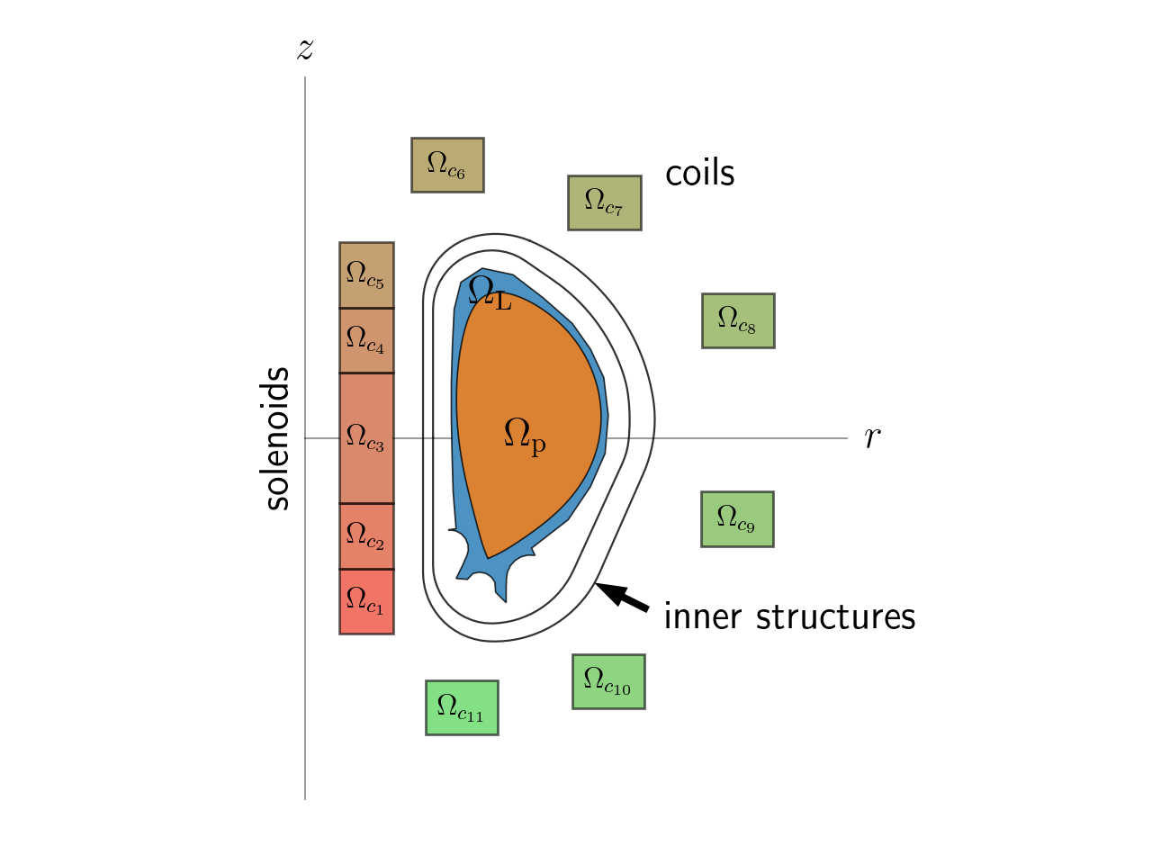
Figure 1: Left: geometry of the problem depicting the $(r,z)$ cross section of a tokamak. The domain contains coils and solenoids, $\Omega_{c_{i}}$, for $i=1,\dots,N_{I}$, a limiter region, $\Omega_{\rm L}$, inside of the first wall, and the plasma region, $\Omega_{p}$, enclosed by $\Omega_{\rm L}$.

Consider a poloidal $(r,z)$ cross section of a tokamak, depicted in Figure 1. Define $\Omega=[0,\infty]\times[-\infty,\infty]$ to be the domain centered with the tokamak geometry. The tokamak is composed of coils, solenoids and inner structures. The coils and solenoids are represented by the subdomains $\Omega_{{\rm C}_{i}}$ labeled by $i=1,\dots,N_{I}$. Let $\Omega_{\rm L}$ be the domain that is enclosed by the first wall. Each of the coils and solenoids has a current, $I_{i}$ for $i=1,\dots,N_{I}$, that is tuned to produce an equilibrium where the plasma, defined by the domain $\Omega_{\rm p}(\psi)\subset\Omega_{\rm L}$, minimizes $d(\partial\Omega_{\rm p}(\psi),\Gamma_{p})$, which represents the distance between the plasma boundary, $\partial\Omega_{\rm p}(\psi)$, and a desired plasma boundary, $\Gamma_{p}$. Additionally, there is a scaling parameter, $\alpha$, involved in the definitions of $f$ and $p$ that is used to control the total plasma current, $I_{\rm p}$. The total plasma current is represented by a domain integral over $\Omega_{\rm p}(\psi)$. This control problem, when combined with boundary conditions for the flux at the axis and far-field, can be summarized as the following PDE-constrained optimization problem.

Problem 1.

Determine the poloidal magnetic flux, $\psi$, and solenoid and coil currents, $I$, and scaling parameter, $\alpha$, that minimizes $d(\partial\Omega_{\rm p}(\psi),\Gamma_{p})$ subject to the constraints

(4a) $$-\frac{1}{\mu r}\Delta^{*}\psi =\begin{cases}rp^{\prime}(\psi)+\frac{1}{\mu r}f(\psi)f^{\prime}(\psi),&\text{\rm in }\Omega_{\rm p}(\psi),\\ I_{i}/|\Omega_{c_{i}}|,&\text{\rm in }\Omega_{c_{i}},\\ 0,&\text{\rm elsewhere in }\Omega_{\infty}\end{cases}$$

(4b) $$\psi(0,z) =0,$$

(4c) $$\lim_{\|(r,z)\|\rightarrow+\infty}\psi(r,z) =0$$

(4d) $$I_{\rm p} =\int_{\Omega_{\rm p}(\psi)}\left(rp^{\prime}(\psi)+\frac{1}{\mu r}{ff^{\prime}}(\psi)\right)\;drdz.$$

The plasma domain, $\Omega_{\rm p}$, is implicitly determined by $\psi$. Let $\psi_{\rm ma}$ and $\psi_{\rm x}$ correspond to the $\psi$ values at the magnetic axis $(r_{\rm ma}(\psi),z_{\rm ma}(\psi))$ and x-point $(r_{\rm x}(\psi),z_{\rm x}(\psi))$, respectively. The magnetic axis corresponds to the global minimum of $\psi$ inside $\Omega_{L}$. When it exists, the x-point is taken to be one of the saddle points of $\psi$ inside the limiter region that has a $\psi$ value closest to $\psi_{\rm ma}$. When there are no candidate saddle points inside $\Omega_{L}$, then this point is chosen to correspond to the maximum value of $\psi$ on $\partial\Omega_{L}$. The level-set of $\psi_{\rm x}$ defines the boundary of the plasma domain.

In order to close the problem, the functions $p$ and $f$ must be supplied. We consider three approaches for defining these functions. The first option is a simple model used in [12] based on Ref. [19]:

Approach 1.

Luxon and Brown Model: the functions $p^{\prime}$ and $ff^{\prime}$ are provided as

(5) $$p^{\prime}(\psi)=\alpha\frac{\beta}{r_{0}}(1-\psi_{N}(\psi)^{\delta})^{\gamma},\qquad f(\psi)f^{\prime}(\psi)=\alpha(1-\beta)\mu r_{0}(1-\psi_{N}(\psi)^{\delta})^{\gamma},$$

where $\psi_{N}(\psi)$ represents a normalized poloidal flux, given by

(6) $$\psi_{N}(\psi)=\frac{\psi-\psi_{\rm ma}(\psi)}{\psi_{\rm x}(\psi)-\psi_{\rm ma}(\psi)}.$$

Here $\alpha$ is a scaling constant that is used to satisfy the constraint (4d). We let $r_{0}=6.2,\,\delta=2,\,\beta=0.5978,\,\gamma=1.395$, using the same coefficients used in [12] for the ITER configuration. This problem is referred to as “inverse static, with given plasma current $I_{\rm p}$” in [12].

Next we consider the Taylor state equilibrium. In a tokamak disruption, if the thermal quench is driven by parallel plasma transport along open magnetic field lines, the plasma current profile is supposed to relax as the result of magnetic reconnection and magnetic helicity conservation. Taylor state corresponds to the extreme case in which $\nabla\times B=\alpha B$ with $\alpha$ a global constant. Substituting the magnetic field representation (2) and the current in MHD (1b) into the Taylor state constraint gives

(7) $$\frac{\partial f}{\partial\psi}\nabla\psi\times\frac{1}{r}e_{\phi}-\frac{1}{r}\left(\Delta^{*}\psi\right)e_{\phi}=\alpha\left[\frac{1}{r}\nabla\psi\times e_{\phi}+\frac{f(\psi)}{r}e_{\phi}\right].$$

Projecting onto two components, one has

(8) $$\frac{\partial f}{\partial\psi} =\alpha,$$

(9) $$-\Delta^{*}\psi =\alpha f(\psi).$$

In the free-boundary Grad–Shafranov equilibrium formulation, $f$ is usually a function of the normalized flux $\psi_{N}(\psi)$. Solving (8), we have

$$f(\psi) =f_{\rm x}-\alpha\left(\psi_{\rm x}-\psi_{\rm ma}\right)+\alpha\left(\psi_{\rm x}-\psi_{\rm ma}\right){\psi}_{N}(\psi)$$

(10) $$=f_{\rm x}+\alpha(\psi-\psi_{\rm x})$$

It is interesting to note that

(11) $$f(\psi_{\rm x})=f\big{|}_{{\psi_{N}(\psi)}=1}=f_{\rm x}$$

is set by the vacuum toroidal field (given by the current in the toroidal field coils). The toroidal field on the magnetic axis has an explicit dependence on $\alpha,$ via

(12) $$f(\psi_{\rm ma})=f\big{|}_{{\psi_{N}(\psi)}=0}=f_{\rm x}+\alpha\left(\psi_{\rm ma}-\psi_{\rm x}\right).$$

On ITER, there is no change in $f_{\rm x}$ over the time period of thermal quench and perhaps current quench as well, so $f_{\rm x}$ is set by the original equilibrium. The factor $\alpha$ sets the total plasma current,

(13) $$I_{\rm p}(\alpha)=\int_{\Omega_{\rm p}(\psi)}\frac{1}{\mu r}{ff^{\prime}}(\psi)\;drdz$$

In other words, we will invert for $\alpha$ at any given total toroidal plasma current $I_{\rm p}.$

In summary, the second option we consider is:

Approach 2.

Taylor State Equilibrium: $p^{\prime}(\psi)=0$ and the diamagnetic function is given by

(14) $$f(\psi)=f_{\rm x}+\alpha(\psi-\psi_{\rm x}),$$

where $f_{\rm x}$ is a constant set by the vacuum toroidal field.

The final option we consider involves some measurement data from a proposed 15MA ITER baseline [18], which relates $p$ and $f$ to $\psi$.

Approach 3.

15MA ITER baseline case: $p^{\prime}$ and $ff^{\prime}$ are provided using tabular data as a function of a normalized poloidal flux. Splines, $S_{p^{\prime}}(\psi_{N})$ and $S_{f}(\psi_{N})$, are fitted to the tabular data and we define the functions as

(15) $$p(\psi)=S_{p^{\prime}}(\psi_{N}(\psi))\qquad f(\psi)=f_{\rm x}+\alpha S_{f}(\psi_{N}(\psi)),$$

where $f_{\rm x}$ is the toroidal field function the separatrix, which is constrained by the total poloidal current in the toroidal field coils outside the chamber wall, and $S_{f}(\psi_{N}(\psi))$ is normalized and centered so that $S_{f}(1)=0$ and $S_{f}(0)=1$. Again, $\alpha$ is a scaling constant that is used to satisfy the constraint (4d)

3 Discretization

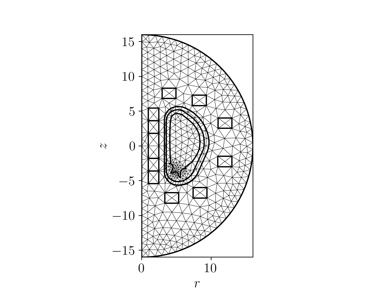
Figure 2: Computational mesh over the region $\Omega$. The geometry of the coils, soilenoids, and inner structures are overlaid over the mesh.

Let $\Omega$ denote the computational domain, represented by the semi-circle $\{r,z:r^{2}+z^{2}\leq R^{2},\;r\geq 0\}$. Figure 2 shows the computational domain and its exemplar coarse mesh. The domain is meshed using 2D elements (i.e., triangles) and the solution, $\psi(r,z)$, is assumed to be in $H^{1}(\Omega)$. Let $\Gamma_{R}$ correspond to the arc of the semi-circle, $\{r,z:r^{2}+z^{2}=R^{2},\;r\geq 0\}$. Additionally, let $v_{i}(r,z)$, $i=1,\dots,N_{\rm dof}$ represent the $i^{\rm th}$ shape function. We wish to solve the following nonlinear equations for $\psi$.

(16) $${\rm a}(\psi,v_{i})=l(I,v_{i}),\qquad i=1,\dots,N_{\rm dof}.$$

Here, $a$ represents the weak form of (4), and contains contributions from the $\Delta^{*}$ operator, plasma terms, and far-field boundary terms.

(17) $$a(\psi,v)=a_{\Delta^{*}}(\psi,v)+a_{\rm plasma}(\psi,v)+a_{\rm far-field}(\psi,v)$$

The terms are given by

(18a) $$a_{\Delta^{*}}(\psi,v)=\; {\int_{\Omega}\frac{1}{\mu r}\nabla\psi\cdot\nabla v\;drdz}$$

(18b) $$a_{\rm plasma}(\psi,v)=\; -{\int_{\Omega_{\rm p}(\psi)}\left(rp^{\prime}(\psi)+\frac{1}{\mu r}f(\psi)f^{\prime}(\psi)\right)v\;drdz}$$

(18c) $$a_{\rm far-field}(\psi,v)=\; \frac{1}{\mu}\int_{\Gamma}\psi(\mathbf{x})N(\mathbf{x})v(\mathbf{x})\;dS(\mathbf{x})$$

$$+\frac{1}{2\mu}\int_{\Gamma}\int_{\Gamma}(\psi(\mathbf{x})-\psi(\mathbf{y}))M(\mathbf{x},\mathbf{y})(v(\mathbf{x})-v(\mathbf{y}))\;dS(\mathbf{x})dS(\mathbf{y}),$$

The far-field terms result from applying appropriate Green’s functions on $\Gamma$ [1] and result in a dense boundary block. These terms use the following definitions

(19) $$M(\mathbf{x},\mathbf{y}) =\frac{k_{\mathbf{x},\mathbf{y}}}{2\pi(\mathbf{x}_{r}\mathbf{y}_{r})^{3/2}}\left(\frac{2-k^{2}_{\mathbf{x},\mathbf{y}}}{2-2k^{2}_{\mathbf{x},\mathbf{y}}}E(k_{\mathbf{x},\mathbf{y}})-K(k_{\mathbf{x},\mathbf{y}})\right),$$

(20) $$N(\mathbf{x}) =\frac{1}{\mathbf{x}_{r}}\left(\frac{1}{\delta_{+}}+\frac{1}{\delta_{-}}-\frac{1}{\rho_{\Gamma}}\right),$$

where $K$ and $E$ are the complete elliptic integrals of the first and second kind, respectively, and

$$\delta_{\pm}=\sqrt{\mathbf{x}_{r}^{2}+(\rho_{\Gamma}\pm\mathbf{x}_{z})^{2}},\qquad k_{\mathbf{x},\mathbf{y}}=\sqrt{\frac{4\mathbf{x}_{r}\mathbf{y}_{r}}{(\mathbf{x}_{r}+\mathbf{y}_{r})^{2}+(\mathbf{x}_{z}-\mathbf{y}_{z})^{2}}}.$$

The form $l$ contains the contribution from the coils, and is given by

(21) $$l(I,v) ={\sum_{i=1}^{N_{I}}\frac{I_{i}}{|\Omega_{{\rm C}_{i}}|}\int_{\Omega_{{\rm C}_{i}}}v\;drdz.}$$

In order to solve (16), we introduce a Newton iteration for $\varphi^{k+1}=\psi^{k+1}-\psi^{k}$. This iteration can be summarized as the linearized system of equations for $\varphi^{k+1}$

(22) $$d_{\psi}(\varphi^{k+1})[{\rm a}(\psi^{k},v_{i})]=l(I,v_{i})-{\rm a}(\psi^{k},v_{i}),\qquad i=1,\dots,N_{\rm dof},$$

where $d_{\psi}(\varphi)$ represents the Gateaux semiderivative in the direction of $\varphi$ where, for a smooth function $g$, is defined by

(23) $$d_{\psi}(\varphi)[g(\psi)]=\lim_{\epsilon\rightarrow 0}\frac{g(\psi+\epsilon\varphi)-g(\psi)}{\epsilon}=\frac{d}{d\epsilon}g(\psi+\epsilon\varphi)\bigg{|}_{\epsilon=0}$$

The Gateaux semiderivative of the operator $a$ is given by

(24) $$d_{\psi}(\varphi)[a(\psi,v)]=d_{\psi}(\varphi)[a_{\Delta^{*}}(\psi,v)]+d_{\psi}(\varphi)[a_{\rm plasma}(\psi,v)]+d_{\psi}(\varphi)[a_{\rm far-field}(\psi,v)].$$

Due to linearity, $d_{\psi}(\varphi)[a_{\Delta^{*}}(\psi,v)]=a_{\Delta^{*}}(\varphi,v)$ and $d_{\psi}(\varphi)[a_{\rm far-field}(\psi,v)]=a_{\rm far-field}(\varphi,v)$. The Gateaux semiderivative of $a_{\rm plasma}$ is given by

$$d_{\psi}(\varphi)[a_{\rm plasma}(\psi,v)]=\; -\int_{\Omega_{\rm p}(\psi)}d_{\psi}(\varphi)\left[\left(rp^{\prime}(\psi)+\frac{1}{\mu r}f(\psi)f^{\prime}(\psi)\right)\right]v\;drdz$$

(25) $$-\int_{\partial\Omega_{\rm p}(\psi)}\bigg{(}rp^{\prime}(\psi)+\frac{1}{\mu r}f(\psi)f^{\prime}(\psi)\bigg{)}|\nabla\psi|^{-1}(\varphi(r_{\rm x}(\psi),z_{\rm x}(\psi))-\varphi)\,v\;ds.$$

See Section A.1 for the derivation.

The derivatives $d_{\psi}(\varphi)[p^{\prime}(\psi)]$ and $d_{\psi}(\varphi)[f(\psi)f^{\prime}(\psi)]$ are nontrivial and depend on the choice for representing these functions. We compute these derivatives analytically using shape calculus, as introduced in [12] for this problem.

Luxon and Brown Model

The semiderivatives of the functions defined in (5) are

(26a) $$d_{\psi}(\varphi)[p^{\prime}(\psi)] =\alpha\frac{\beta}{r_{0}}\gamma\delta(1-\psi_{N}(\psi)^{\delta})^{\gamma-1}\psi_{N}(\psi)^{\delta-1}d_{\psi}(\varphi)[\psi_{N}(\psi)]$$

(26b) $$d_{\psi}(\varphi)[f(\psi)f^{\prime}(\psi)] =\alpha(1-\beta)\mu r_{0}\gamma\delta(1-\psi_{N}(\psi)^{\delta})^{\gamma-1}\psi_{N}(\psi)^{\delta-1}d_{\psi}(\varphi)[\psi_{N}(\psi)]$$

where

(27) $$d_{\psi}(\varphi)[\psi_{N}(\psi)]=\frac{\varphi-(1-\psi_{N}(\psi))\varphi(r_{\rm ma}(\psi),z_{\rm ma}(\psi))-\psi_{N}(\psi)\varphi(r_{\rm x}(\psi),z_{\rm x}(\psi))}{\psi_{\rm x}-\psi_{\rm ma}}.$$

The nontrivial derivation of (27) involves shape calculus and is provided in Section A.2.

Taylor Equilibrium

The right-hand-side terms are given by

(28) $$f(\psi)f^{\prime}(\psi)=\alpha\left[f_{\rm x}+\alpha(\psi-\psi_{\rm x})\right].$$

The relevant semiderivative is given by

(29) $$d_{\psi}(\varphi)[f(\psi)f^{\prime}(\psi)] =\alpha^{2}(1-d_{\psi}(\varphi)\psi_{\rm x})=\alpha^{2}(1-\varphi(r_{\rm x}(\psi),z_{\rm x}(\psi))).$$

Note that the result $d_{\psi}(\varphi)\psi_{\rm x}=\varphi(r_{\rm x}(\psi),z_{\rm x}(\psi))$, which is derived in Section A.2, is used to simplify the result.

15MA ITER baseline case

We have

(30) $$f(\psi)f^{\prime}(\psi)=\frac{1}{\psi_{\rm ma}-\psi_{\rm x}}\alpha(f_{\rm x}+\alpha S_{f}(\psi_{N}(\psi)))S_{f}^{\prime}(\psi_{N}(\psi)).$$

Using the results from Section A.2, the semiderivative for $ff^{\prime}$ is given by

(31) $$d_{\psi}(\varphi)[f(\psi)f^{\prime}(\psi)]=\; \frac{1}{\psi_{\rm ma}-\psi_{\rm x}}\alpha^{2}S_{f}^{\prime}(\psi_{N}(\psi)))^{2}d_{\psi}(\varphi)[\psi_{N}(\psi)]$$

$$+\frac{1}{\psi_{\rm ma}-\psi_{\rm x}}\alpha(f_{\rm x}+\alpha S_{f}(\psi_{N}(\psi)))S_{f}^{\prime\prime}(\psi_{N}(\psi))d_{\psi}(\varphi)[\psi_{N}(\psi)]$$

$$-\frac{\varphi_{\rm ma}-\varphi_{\rm x}}{(\psi_{\rm ma}-\psi_{\rm x})^{2}}\alpha(f_{\rm x}+\alpha S_{f}(\psi_{N}(\psi)))S_{f}^{\prime}(\psi_{N}(\psi)).$$

The semiderivative for $p^{\prime}$ is given by

(32) $$d_{\psi}(\varphi)[p^{\prime}(\psi)] =S_{p^{\prime}}^{\prime}(\psi_{N}(\psi))d_{\psi}(\varphi)[\psi_{N}(\psi)].$$

Due to the presence of $\varphi_{\rm x}$ and $\varphi_{\rm ma}$ in (25), the discrete matrix formed by building $d_{\psi}(\varphi)[a_{\rm plasma}(\psi,v)]$ contains nonzeros in columns corresponding to the indices of the magnetic axis and x-point along rows corresponding to indices in $\Omega_{p}(\psi)$. We note that the resulting matrix is not symmetric.

3.1 Location of $\mathbf{x}_{\rm ma}$ and $\mathbf{x}_{\rm x}$ and Determination of $\Omega_{\rm p}$

In this section, the algorithms for locating the magnetic axis ($\mathbf{x}_{\rm ma}$) and magnetic x-point ($\mathbf{x}_{\rm x}$) and determining the elements that contain $\Omega_{\rm p}$ are described. We assume that the connectivity of adjacent mesh vertices is available in a convenient data structure, such as a map or dictionary. Additionally, we assume that each vertex in $\Omega_{\rm L}$ or on $\partial\Omega_{\rm L}$ is marked and collected into a list. First, all of the marked vertices in $\Omega_{\rm L}$ and $\partial\Omega_{\rm L}$ are searched to determine the maximal and minimal values for $\psi$ in addition to any saddle points in $\psi$. $\mathbf{x}_{\rm ma}$ is set to be the location of the vertex corresponding to the minimum $\psi$ value. If one or more vertices are found to be saddle points, $\mathbf{x}_{\rm x}$ is set to be the location of the saddle point vertex with a $\psi$ value closest to $\psi_{\rm ma}$. Otherwise, $\mathbf{x}_{\rm x}$ is set to be the location of the vertex corresponding to the maximum $\psi$ value.

Saddle points are determined using the following algorithm. Let $\psi_{o}$ be the function value at a candidate vertex and let $\psi_{1},\dots,\psi_{N_{v}}$ be function values of adjacent vertices ordered clock-wise. The candidate vertex is marked as an $H^{1}$ saddle point if the sequence $\psi_{1}-\psi_{o},\dots,\psi_{N_{v}}-\psi_{o},\psi_{1}-\psi_{o}$ contains 4 or more sign changes.

After determining $\mathbf{x}_{\rm ma}$ and $\mathbf{x}_{\rm x}$, a tree search is performed to determine the vertices belonging to or adjacent to $\Omega_{\rm p}$. A dynamic queue is initially populated with the vertex at $\mathbf{x}_{\rm ma}$. Until the queue is empty, vertices in the queue are removed from the queue and its adjacent vertices are investigated. If a neighboring vertex has a $\psi$ value in between $\psi_{\rm ma}$ and $\psi_{\rm x}$, then it is marked to be inside of $\Omega_{\rm p}$ and added to the queue. Otherwise, it is marked to be adjacent to $\Omega_{\rm p}$. Domain integrals over $\Omega_{\rm p}$ are evaluated over each element containing vertices in or adjacent to $\Omega_{\rm p}$. When the vertex is adjacent to $\Omega_{\rm p}$, the integrand is set to be zero.

3.2 Adaptive Mesh Refinement

Adaptive mesh refinement (AMR) is applied to increase the mesh resolution in areas of high priority according to the Zienkiewicz-Zhu (ZZ) error estimation procedure [24, 25]. An element is marked for refinement when its local error estimate is greater than a globally defined fraction of the total error estimate. More specifically, we divide the mesh into two regions, $\Omega_{\rm L}$, which contains the plasma region, and $\Omega\backslash\Omega_{\rm L}$, which have their own respective refinement thresholds.

We explore two approaches. In the first approach, we use the computed solution $\psi$ and the elliptic operator from the Grad–Shafranov equation in the error estimate. Specifically, the error of the ZZ estimator at an element $K$ can be estimated as

$$\eta_{K}^{2}(\psi_{h})=\int_{K}\|G[\psi_{h}]-\tilde{\nabla}\psi_{h}\|^{2}\;drdz$$

where $G[\psi_{h}]$ denotes the smoother version of the flux, and $\tilde{\nabla}\psi_{h}$ is a numerical interpolated flux. Here $G[\psi_{h}]$ is solved from the diffusion operator $\frac{1}{\mu r}\Delta^{*}$, and $\tilde{\nabla}:=\frac{1}{\mu r}[\partial_{r},\,\partial_{z}]^{T}$. This is a well defined error estimator for the proposed problem, since the problem is of an elliptic nature. However, this error estimator may prioritize the solution of $\psi$ instead of $\tilde{\nabla}\psi$, latter of which is more interesting as it becomes the components of $B$.

To accommodate the need of resolving more interesting physics, we also consider using the toroidal $B$ field as the input in the ZZ estimator. We first reconstruct the toroidal $B$ field from $f(\psi)$ and then use this as the input in the ZZ estimator. This will naturally prioritize the jump in the toroidal current of the equilibrium. Note that this approach leads to a feature-based indictor, which in practice can work well for the need.

4 Optimization

Consider a curve $\Gamma_{\rm p}$ describing the shape of a desired plasma boundary. The goal is to find the poloidal magnetic flux $\psi(r,z)$ coil currents, $I_{j}$, $j=1,\dots,M$, and scaling parameter, $\alpha$, such that some objective function penalizing the distance between $\partial\Omega_{\rm p}$ and $\Gamma_{\rm p}$,

(33) $$g(\psi)=d(\partial\Omega_{\rm p}(\psi),\Gamma_{\rm p}),$$

is minimized subject to the following constraints. The first constraint enforces that $\psi$ is a solution to the Grad–Shafranov equations, which are summarized symbolically by the system of equations,

(34) $$B(\psi)-F(I)=0.$$

In addition to the above constraint, we enforce the following constraint to set the plasma current equal to a desired value of $I_{\rm p}$,

(35) $${\int_{\Omega_{\rm p}(\psi)}\left(rp^{\prime}(\psi)+\frac{1}{\mu r}{ff^{\prime}}(\psi)\right)\;drdz}=I_{\rm p}.$$

For well-posedness, we add the Tikhonov regularization term,

(36) $$h(I)=\frac{1}{2}\sum_{j=1}^{N_{I}}w_{j}I_{j}^{2},$$

which penalizes solutions with large currents. There are $N_{I}$ independent currents that can be controlled. The optimization problem can be written as

$$\min_{\psi,\,\alpha,\,I}\qquad g(\psi)+h(I),$$

s.t. $$B(\psi)-F(I)=0,$$

$${\int_{\Omega_{\rm p}(\psi)}\left(rp^{\prime}(\psi)+\frac{1}{\mu r}{ff^{\prime}}(\psi)\right)\;drdz}=I_{\rm p}.$$

We now discuss the choice of objective function. Points $x_{1},\dots,x_{N_{c}}$ are chosen from a reference plasma boundary curve. Since $\psi_{N}=1$ defines the contour that contains the x-point, we define our objective to penalize when the solution along the reference curve is not on the contour of the x-point,

(37) $$g(\psi)=\frac{1}{2}\sum_{i=1}^{N_{c}}(\psi_{N}(\psi(x_{i}))-1)^{2}.$$

Note that this constraint is different from that in [12], and becomes fully nonlinear.

4.1 Fully Discretized System

Consider the decomposition of $\psi$ into linear algebraic degrees of freedom, $y$. Let $y_{n}$ be the coefficient for the $n^{\rm th}$ shape basis function $v_{n}(r,z)$. Then

(38) $$\psi(r,z)=\sum_{n=1}^{N_{\rm dof}}y_{n}v_{n}(r,z).$$

We redefine the current variables as $u_{j}=I_{j}$ for $j=1,\dots,N_{I}$. In terms of linear algebraic variables, we rewrite the objective function as

$$\min_{\psi,I}\qquad G(y)+R(u),$$

s.t. $$B(y,\alpha)-Fu=0,$$

$$C(y,\alpha)-I_{\rm p}=0,$$

where $G(y),R(u)\in\mathbb{R}$ represent the objective function and regularization, $B(y,\alpha)\in\mathbb{R}^{N_{\rm dof}}$ represents the solution operator, $F\in\mathbb{R}^{N_{\rm dof}\times N_{I}}$ represents the coil contributions, and $C(y,\alpha)\in\mathbb{R}$ represents the plasma current. The regularizer, $R(u)$, is defined as

(39) $$R(u)=\frac{1}{2}u^{T}Hu.$$

A simple choice is to choose $H=\epsilon I$, where $\epsilon$ is small (e.g. $\epsilon\sim 10^{-12}$).

The Lagrangian for the problem is given by

(40) $$\mathcal{L}=G(y)+R(u)+p^{T}(B(y,\alpha)-Fu)+\lambda(C(y,\alpha)-I_{\rm p})$$

where $p$ and $\lambda$ are Lagrange multipliers. The fixed point $(y^{*},u^{*},\alpha^{*},p^{*},\lambda^{*})$ is the solution to the equations

(41a) $$G_{y}(y)+B_{y}(y,\alpha)^{T}p+C_{y}(y,\alpha)\lambda =0,$$

(41b) $$Hu-F^{T}p =0,$$

(41c) $$B(y,\alpha)-Fu =0,$$

(41d) $$B_{\alpha}(y,\alpha)^{T}p+C_{\alpha}(y,\alpha)\lambda =0$$

(41e) $$C(y,\alpha) =I_{\rm p},$$

We introduce a Newton iteration to address (41). Let $(y^{n},u^{n},p^{n},\alpha^{n},\lambda^{n})$ represent the solution state at iteration $n$ and let $\Delta$ represent a forward difference operator (i.e., $\Delta y^{n}:=y^{n+1}-y^{n}$). The iteration is defined as

(57) $$\left[\begin{array}[]{ccccc}G_{yy}(y^{n})&0&B_{y}(y^{n},,\alpha^{n})^{T}&0&C_{y}(y,\alpha)\\ 0&H&-F^{T}&0&0\\ B_{y}(y^{n},\alpha^{n})&-F&0&B_{\alpha}(y,a)&0\\ 0&0&B_{\alpha}(y,\alpha)^{T}&0&C_{\alpha}(y,\alpha)\\ C_{y}(y,\alpha)^{T}&0&0&C_{\alpha}(y,\alpha)&0\end{array}\right]\left[\begin{array}[]{c}\Delta y^{n}\\ \Delta u^{n}\\ \Delta p^{n}\\ \Delta\alpha^{n}\\ \Delta\lambda^{n}\end{array}\right]=\left[\begin{array}[]{c}b_{1}^{n}\\ b_{2}^{n}\\ b_{3}^{n}\\ b_{4}^{n}\\ b_{5}^{n}\end{array}\right],$$

where

(68) $$\left[\begin{array}[]{c}b_{1}^{n}\\ b_{2}^{n}\\ b_{3}^{n}\\ b_{4}^{n}\\ b_{5}^{n}\end{array}\right]=-\left[\begin{array}[]{c}G_{y}(y^{n})+B_{y}(y^{n},\alpha^{n})^{T}p^{n}+C_{y}(y^{n},\alpha^{n})\lambda^{n}\\ Hu^{n}-F^{T}p^{n}\\ B(y^{n},\alpha^{n})-Fu^{n}\\ B_{\alpha}(y^{n},\alpha^{n})^{T}p^{n}+C_{\alpha}(y^{n},\alpha^{n})\lambda^{n}\\ C(y^{n},\alpha^{n})-I_{\rm p}\end{array}\right].$$

We eliminate $\Delta u^{n}$, $\Delta\alpha^{n}$, and $\Delta\lambda^{n}$ algebraically to arrive at a block system given by

(75) $$\left[\begin{array}[]{cc}B_{y}-\frac{1}{C_{\alpha}}B_{\alpha}C_{y}^{T}&-FH^{-1}F^{T}\\ G_{yy}&B_{y}^{T}-\frac{1}{C_{\alpha}}C_{y}B_{\alpha}^{T}\end{array}\right]\left[\begin{array}[]{c}\Delta y\\ \Delta p\end{array}\right]=\left[\begin{array}[]{c}b_{3}+FH^{-1}b_{2}-\frac{1}{C_{\alpha}}B_{\alpha}b_{5}\\ b_{1}-\frac{1}{C_{\alpha}}C_{y}b_{4}\end{array}\right].$$

For notational convenience, the functional dependence of the operators and the superscripts denoting the iteration number are omitted. The original system (57) is symmetric while the system (75) after the block factorization is non-symmetric. Although the system (75) can be easily symmetrized by reordering $\Delta y$ and $\Delta p$, this does not help the preconditioning strategy that will be discussed in the next section.

4.2 Computation of Objective Function and its Derivatives

The iteration in (75) requires the computation of gradient and Hessian of the objective function. In terms of the linear algebraic variables, the objective function is given by

(76) $$G(y)=\frac{1}{2}\sum_{i=1}^{N_{c}}(\bar{y}_{i}-1)^{2}$$

where $\bar{y}_{i}$ represents the discrete analog to $\psi_{N}(\psi(x_{i}))$. For $H^{1}(\Omega)$ functions represented on 2D triangular elements, off-nodal function values can be expressed as an interpolation of the nodal values. For each control point, $x_{i}$, the bounding vertices are located and their indices are labeled as $J_{1}^{(i)},J_{2}^{(i)},J_{3}^{(i)}$. Additionally, corresponding interpolation coefficients, $\alpha_{J_{1}^{(i)}},\alpha_{J_{2}^{(i)}},\alpha_{J_{3}^{(i)}},$ are computed. We therefore define $\bar{y}_{i}$ as

(77) $$\bar{y}_{i}=\frac{\sum_{m=1}^{3}\alpha_{J_{m}^{(i)}}y_{J_{m}^{(i)}}-y_{\rm ma}}{y_{\rm x}-y_{\rm ma}},$$

where $y_{\rm ma}$ and $y_{\rm x}$ correspond to the nodal values of the magnetic axis and x-point. The gradient and Hessian of the objective function are defined through

(78a) $$\frac{\partial}{\partial y_{m}}G(y) =\sum_{i=1}^{N_{c}}(\bar{y}_{i}-1)\frac{\partial\bar{y}_{i}}{\partial y_{m}},$$

(78b) $$\frac{\partial^{2}}{\partial y_{m}\partial y_{n}}G(y) =\sum_{i=1}^{N_{c}}\left((\bar{y}_{i}-1)\frac{\partial^{2}\bar{y}_{i}}{\partial y_{m}\partial y_{n}}+\frac{\partial\bar{y}_{i}}{\partial y_{m}}\frac{\partial\bar{y}_{i}}{\partial y_{n}}\right).$$

The above require the definitions of the following derivatives.

(79a) $$\frac{\partial\bar{y}_{i}}{\partial y_{m}} =\frac{1}{y_{\rm x}-y_{\rm ma}}\left(\sum_{m=1}^{3}\alpha_{J_{m}^{(i)}}\frac{\partial y_{J_{m}^{(i)}}}{\partial y_{m}}-\frac{\partial y_{\rm ma}}{\partial y_{m}}\right)-\frac{1}{y_{\rm x}-y_{\rm ma}}\left(\frac{\partial y_{\rm x}}{\partial y_{m}}-\frac{\partial y_{\rm ma}}{\partial y_{m}}\right)\bar{y}_{i},$$

(79b) $$\frac{\partial^{2}\bar{y}_{i}}{\partial y_{m}\partial y_{n}} =\frac{1}{y_{\rm ma}-y_{\rm x}}\left(\left(\frac{\partial y_{\rm x}}{\partial y_{n}}-\frac{\partial y_{\rm ma}}{\partial y_{n}}\right)\frac{\partial\bar{y}_{i}}{\partial y_{m}}+\left(\frac{\partial y_{\rm x}}{\partial y_{m}}-\frac{\partial y_{\rm ma}}{\partial y_{m}}\right)\frac{\partial\bar{y}_{i}}{\partial y_{n}}\right)$$

5 Preconditioning Approach

At each iteration, the system is given by

(86) $$\left[\begin{array}[]{cc}B&A\\ C&B^{T}\end{array}\right]\left[\begin{array}[]{c}\Delta p\\ \Delta y\end{array}\right]=\left[\begin{array}[]{c}c_{1}\\ c_{2}\end{array}\right],$$

where the block operators are given by

(87) $$A=G_{yy},\qquad B=B_{y}^{T}-\frac{1}{C_{\alpha}}C_{y}B_{\alpha}^{T},\qquad C=-FH^{-1}F^{T},$$

and the right hand side block vectors are defined to be

(88) $$c_{1}=b_{1}-\frac{1}{C_{\alpha}}C_{y}b_{4},\qquad c_{2}=b_{3}+FH^{-1}b_{2}-\frac{1}{C_{\alpha}}B_{\alpha}b_{5}.$$

$A$ and $-C$ are both symmetric positive semi-definite and $B$ and $B^{T}$ are both invertible. The operator $B$ incorporates the contribution from the elliptic operator, plasma terms, and boundary conditions in $B_{y}^{T}$ and a rank-one perturbation in $-\frac{1}{C_{\alpha}}C_{y}B_{\alpha}^{T}$ that is dense over the plasma degrees of freedom. The operator $C$ is dense over the coil degrees of freedom and the operator $A$ only contains non-zero entries nearby the plasma control points.

At each Newton iteration, (86) is solved using FGMRES [22]. The following discussion summarizes the preconditioning approach. In developing a preconditioner, our hypothesis is that the problem is dominated primarily by the elliptic part of the diagonal operators. This motivates a block diagonal preconditioner using algebraic multigrid (AMG).

(91) $$\text{Block Diagonal PC:}\qquad\mathcal{P}^{-1}_{\rm BD} =\left[\begin{array}[]{cc}{\rm AMG}(B_{y}^{T})&0\\ 0&{\rm AMG}(B_{y})\end{array}\right].$$

This version uses two evaluations of AMG per Krylov solver iteration. Another level of approximation involves incorporating one of the off-diagonal blocks.

(94) $$\text{Block Upper Triangular PC:}\qquad\mathcal{P}^{-1}_{\rm BUT} =\left[\begin{array}[]{cc}{\rm AMG}\left(B_{y}^{T}\right)&D\\ 0&{\rm AMG}\left(B_{y}\right)\end{array}\right],$$

(97) $$\text{Block Lower Triangular PC:}\qquad\mathcal{P}^{-1}_{\rm BLT} =\left[\begin{array}[]{cc}{\rm AMG}\left(B_{y}^{T}\right)&0\\ E&{\rm AMG}\left(B_{y}\right)\end{array}\right].$$

Here, $D=-{\rm AMG}(B_{y}^{T})\,A\,{\rm AMG}(B_{y})$ and $E=-{\rm AMG}(B_{y})\,C\,{\rm AMG}(B_{y}^{T})$. These preconditioners also require two evaluations of AMG per Krylov solver iteration. For each preconditioner, we consider their performance for the choice of AMG cycle type (either V-cycle or W-cycle) and number of AMG iterations.

Remark 5.1.

The system can be solved by calling AMG as the preconditioner for the whole block system. A biharmonic example from the hypre library [13] considers the same solver option. However, this is found to be less efficient than the proposed preconditioning strategy.

Remark 5.2.

In an attempt to address the system (86), we also considered its equivalent version by reordering the two variables. This problem can be through as a generalized saddle point problem. Although a Hermitian and skew-Hermitian splitting (HSS) preconditioner proposed in [4] can be modified to work well as the outer solver, it is challenging to address one of the split systems. This is related to the fact that the smoother for the direct discretization of a biharmonic operator is not easy to construct.

Inexact Newton Method

An inexact Newton procedure based on [10] is used to determine the relative tolerance for the FGMRES solver. Let $e_{n}$ be the global error norm at step $n$ and let $\eta_{\max}$ be the maximum relative tolerance, then we choose the relative tolerance at the next Newton iteration to be given by

(98) $$\eta_{n}=\min\left(\gamma\left(\frac{e_{n}}{e_{n-1}}\right)^{\theta},\eta_{\max}\right),$$

where $\theta=(1+\sqrt{5})/2$ and $\gamma\approx 1$.

6 Implementation

Our algorithm for solving the Grad–Shafranov equation is implemented using the freely available C++ library MFEM [20, 3]. In this section, a few of the implementation details are discussed. The geometry is meshed using triangular elements using the Gmsh software [11]. The linearized system of equations in (22) is implemented using a combination of built-in and custom integrators. In particular, the bilinear form associated with (18c) is built using a custom integrator and the contribution to $B_{y}$ from (25) is implemented by building a custom sparse matrix. The block system in (86) and the preconditioners in (91)–(94) are implemented as nested block operators. Hypre’s algebraic multigrid preconditioners [13] are used to precondition the matrices $B_{y}$ and $B_{y}^{T}$ and MFEM’s built in FGMRES implementation is used to solve the block system. MFEM’s built in Zienkiewicz-Zhu error estimation procedure is used to refine the mesh at each AMR level. The implementation of the solver in this paper and the scripts used to generate the results of this paper are currently maintained in the tds-gs branch of MFEM at https://github.com/mfem/mfem/tree/tds-gs. During the preparation of this paper, we used MFEM version 4.5.3 and Hypre version 2.26.0.

7 Results

In this section, we demonstrate our new solver using the three discussed approaches for handling the right-hand-side of (4). First we perform a study to test the performance of the new preconditioner. We then devise a case study to show the benefit of using adaptive mesh refinement.

7.1 Preconditioner Performance

We consider the Luxon and Brown model, Taylor state equilibrium, and the 15MA ITER baseline case. For all cases, an initial guess was provided from a proposed ITER discharge at 15MA toroidal plasma current [18], which carries the ITER reference number ABT4ZL. The initial solution for $\psi$ is provided in the domain $(r,z)\in[3,10]\times[-6,6]$ and shown in Figure 3. The initial guess for coil currents is shown in the table of Figure 3. 100 control points along the plasma boundary are chosen for the objective function. The magnetic permeability is chosen to be $\mu=1.25663706144\cdot 10^{-6}$ and the target plasma current is set to $I_{\rm p}=15$ MA. For all cases, the Newton relative tolerance was set to $10^{-6}$. Problem specific solver settings are provided in Table 1. The regularization coefficient, $\epsilon$, maximum Krylov relative tolerance, $\eta_{\max}$, initial uniform refinements, and total AMR levels were manually varied based on the problem.

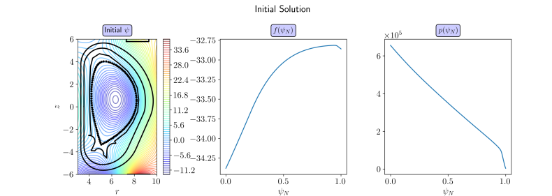
Initial Coil Currents Center Solenoids Poloidal Flux Coils $I_{1}$ 1.143284e+03 $I_{6}$ -4.552585e+06 $I_{2}$ -2.478694e+04 $I_{7}$ 3.180596e+06 $I_{3}$ -3.022037e+04 $I_{8}$ 5.678096e+06 $I_{4}$ -2.205664e+04 $I_{9}$ 3.825538e+06 $I_{5}$ -2.848113e+03 $I_{10}$ 1.066498e+07 $I_{11}$ -2.094771e+07

Figure 3: Details of the reference solution used for the initial guess. Left: initial field for $\psi$. Middle left: line plot of $f(\psi_{N})$. Middle right: line plot of $p(\psi_{N})$. Right: initial coil currents.

Table 1: Solver settings chosen for each problem in Section 7.1. $\epsilon$ corresponds to the regularization coefficient in $H=\epsilon I$, defined in (39). $\eta_{\max}$ is the maximum Krylov relative tolerance used in (98). Also reported is the number of uniform refinements performed on the initial mesh and the number of AMR levels used in the solver.

	Luxon and Brown	Taylor State	15MA ITER
$\epsilon$	1e-12	1e-12	1e-14
$\eta_{\max}$	1e-6	1e-4	1e-6
initial uniform refinements	1	0	2
AMR levels	1	4	0

Table 2 summarizes the performance of the various preconditioner options chosen in terms of number of Newton iterations and outer FGMRES iterations. The number of Newton iterations on the initial mesh are reported in addition to the average number of Newton iterations for each subsequent AMR level. For the majority of cases considered, 4-8 Newton iterations are required to reach an error tolerance of $10^{-6}$. The notable exception includes applying multiple iterations of a W-cycle for the Luxon and Brown model where performance degradation is observed for all preconditioners. Excluding the cases with performance degradation, monotonic improvements in the average number of iterations are seen by either moving from the block-diagonal PC to one of the block triangular PCs, going from a V-Cycle to a W-Cycle, and increasing the number of AMG iterations. While performance is improved with more iterations, there are diminishing returns due to the extra cost of additional AMG iterations. We do not observe a significant difference in performance between the upper block triangular and the lower block triangular PCs.

Table 2: Summary of Newton and FGMRES iterations for the block system in (86) using the block diagonal, upper block triangular, and lower block triangular preconditioners for various combinations of AMG iterations and cycle type. The results are reported in the format $(a_{1},\bar{a})\,b$ or $(a_{1})\,b$, where $a_{1}$ is the number of Newton iterations on the initial mesh, $\bar{a}$ is the average number of Newton iterations on subsequent AMR levels and $b$ is the average number of FGMRES iterations.

Luxon and Brown

Block Diagonal PC
Iterations	V-Cycle	W-Cycle
1	(5, 2.0) 91.0	(5, 2.0) 48.4
3	(5, 2.0) 57.7	(5, 2.0) 40.3
5	(5, 2.0) 47.1	(15, 2.0) 44.5
10	(5, 2.0) 37.4	–

Upper Block Triangular PC
Iterations	V-Cycle	W-Cycle
1	(5, 2.0) 81.4	(5, 2.0) 38.3
3	(5, 2.0) 47.0	(5, 2.0) 32.4
5	(5, 2.0) 36.1	(17, 2.0) 29.0
10	(5, 2.0) 26.9	–

Lower Block Triangular PC
Iterations	V-Cycle	W-Cycle
1	(5, 2.0) 81.3	(5, 2.0) 37.7
3	(5, 2.0) 47.0	(5, 2.0) 38.1
5	(5, 2.0) 36.0	(20, 2.0) 29.8
10	(5, 2.0) 26.4	–

Taylor State Equilibrium

Block Diagonal PC
Iterations	V-Cycle	W-Cycle
1	(5, 2.0) 69.5	(5, 2.0) 38.2
3	(5, 2.0) 46.4	(4, 2.0) 30.4
5	(4, 2.0) 41.1	(4, 2.0) 28.3
10	(4, 2.2) 35.2	(4, 2.0) 26.9

Upper Block Triangular PC
Iterations	V-Cycle	W-Cycle
1	(8, 2.0) 53.8	(5, 2.0) 27.0
3	(5, 2.2) 36.4	(5, 2.0) 18.8
5	(5, 2.2) 29.1	(4, 2.0) 16.7
10	(5, 2.2) 22.7	(4, 2.0) 14.6

Lower Block Triangular PC
Iterations	V-Cycle	W-Cycle
1	(5, 2.0) 59.4	(5, 2.0) 27.5
3	(5, 2.2) 36.9	(4, 2.0) 19.6
5	(4, 2.0) 28.8	(4, 2.0) 17.4
10	(4, 2.2) 23.5	(4, 2.0) 15.9

15MA ITER Case

Block Diagonal PC
Iterations	V-Cycle	W-Cycle
1	(7) 176.1	(7) 67.7
3	(7) 107.3	(7) 46.4
5	(8) 85.6	(7) 40.6
10	(7) 63.9	(7) 35.7

Upper Block Triangular PC
Iterations	V-Cycle	W-Cycle
1	(7) 166.3	(7) 56.4
3	(7) 96.1	(7) 34.6
5	(7) 74.4	(7) 28.7
10	(7) 52.3	(7) 23.9

Lower Block Triangular PC
Iterations	V-Cycle	W-Cycle
1	(7) 167.0	(7) 56.7
3	(7) 96.6	(7) 35.3
5	(7) 74.7	(7) 29.6
10	(7) 52.9	(7) 24.7

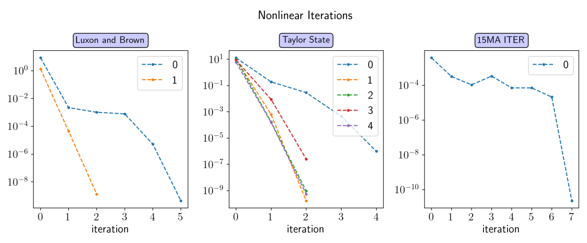
Figure 4: Newton iteration history for each AMR refinement of solution corresponding to the upper block triangular preconditioner with 10 AMG V-Cycle iterations for Luxon and Brown and 10 AMG W-Cycle iterations for the Taylor State and 15MA ITER.

On subsequent AMR levels, an average of only 2 Newton iterations are generally required. The convergence of the Newton iteration for a few selected cases is shown in Figure 4. We note that the convergence rate of the latter AMR iteration becomes much better due to a better initial guess from the previous solve being used, highlighting the power of AMR. Finally, the computed solutions corresponding to the Luxon and Brown model, Taylor state equilibrium, and 15MA ITER case are shown in Figures 5, 6, and 7.

In summary, we found that the proposed block triangular preconditioner with 3 W-cycles performs well in most cases, providing a good balance between the number of iterations and the solve time. In the rare cases when the W-cycle preconditioner fails, a block triangular preconditioner with 3 to 5 V-cycles can be a more robust choice. We also found that fewer nonlinear iterations are required after each application of AMR.

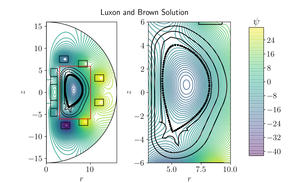
Figure 5: Luxon and Brown solution. Left: full domain. Right: zoomed in domain.

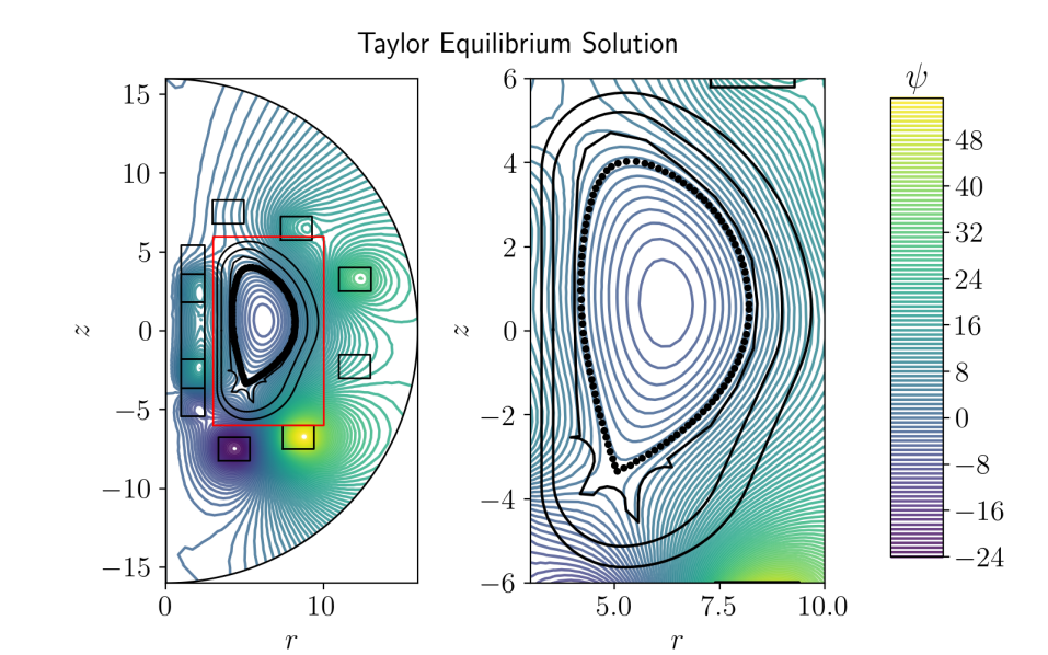
Figure 6: Taylor state equilibrium solution. Left: full domain. Right: zoomed in domain.

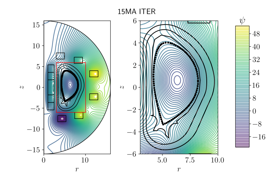
Figure 7: 15MA ITER solution. Left: full domain. Right: zoomed in domain.

7.2 Adaptive Mesh Refinement Case Studies

We demonstrate two different strategies for adaptive mesh refinement. The first approach is to apply the error estimator to the solution $\psi$ at the end of each Newton iteration. Based on our experimentation, the error estimator typically prioritizes the regions near the coils due to the presence of sharper gradients in $\psi$. Due to this, we set a more aggressive threshold according to Section 3.2 in the limiter region to balance refinement near the plasma and near the coils. For the first example, we consider four levels of AMR for the Taylor state equilibrium. The meshes are shown in Figure 8. The refinement targeted regions of large gradients near the coils and specific patches in the limiter region.

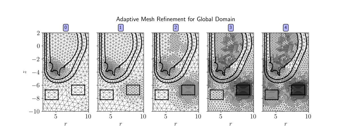
Figure 8: Four levels of AMR applied globally to $\psi$ for the Taylor equilibrium solution.

We also demonstrate an alternative approach where we use $f(\psi)$, which is discontinuous across the plasma boundary, in the error estimator. This approach can be used to increase the resolution along the plasma boundary. For this case, we also consider four levels of AMR for the Taylor state equilibrium. The meshes are shown in Figure 9. The refinement targets the region in the neighborhood around the control points.

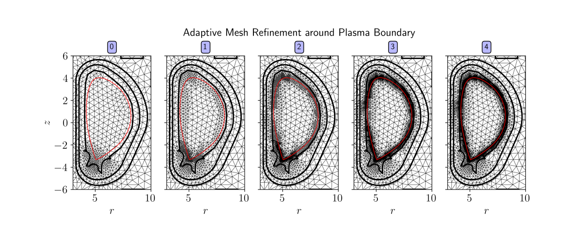
Figure 9: Four levels of AMR applied to $f(\psi)$, which is discontinuous across the plasma boundary. The solid red curve connects the control points used to optimize the plasma boundary.

8 Conclusions

In this work, we develop a Newton-based free-boundary Grad–Shafranov solver based on adaptive finite elements, block preconditioning strategies and algebraic multigrid. A challenging optimization problem to seek a free-boundary equilibrium has been successfully addressed. To seek an efficient and practical solver, we focus on exploring different preconditioning strategies and leveraging advanced algorithms such as AMR and scalable finite elements. We identify several simple but effective preconditioning options for the linearized system. We also demonstrate that the AMR algorithm helps to resolve the local features and accelerates the nonlinear solver. The resulting solver is particularly effective to seek the Taylor state equilibrium that is needed in practical tokamak simulations of vertical displacement events in a post-thermal-quench plasma. Such an equilibrium was impossible to solve by our previous Picard-based solver. In our Newton based approach, we demonstrated that the nonlinear residual can be robustly reduced to 1e-6 and lower in a small handful of iterations. Although a good preconditioner strategy is identified, we note that the performance of the preconditioner have some room for improvement. A potential improvement might be to design a good smoother strategy for the coupled system or its Schur complement. Another future direction is to incorporate the mesh generator into the solver loop, which may address the potentially large change of the plasma domain and can resolve the separatrix dynamically. Such a feature has been under active development in MFEM.

Appendix A Appendix

We provide the details of computing the Gateaux semiderivatives of two exemplar terms using shape calculus. The idea of using shape calculus in the Grad–Shafranov solver was first proposed in [12]. However, the details of the derivation for the shape calculus were not provided in [12]. Here we provide all the necessary details and derivations for the purpose of reproduction.

A.1 Gateaux Semiderivative of $a_{\rm plasma}$

We first apply the definition of the Gateaux semiderivative,

$$d_{\psi}(\varphi)[a_{\rm plasma}(\psi,v)]=-\frac{d}{d\epsilon}\bigg{(}\int_{\Omega_{\rm p}(\psi+\epsilon\varphi)}\bigg{(} rp^{\prime}(\psi+\epsilon\varphi)$$

$$\;+\frac{1}{\mu r}f(\psi+\epsilon\varphi)f^{\prime}(\psi+\epsilon\varphi)\bigg{)}v\;drdz,\bigg{)}\bigg{|}_{\epsilon=0}$$

Using the Leibniz integral rule, the term becomes

$$d_{\psi}(\varphi)[a_{\rm plasma}(\psi,v)]=\; -\int_{\Omega_{\rm p}(\psi)}d_{\psi}(\varphi)\left[\left(rp^{\prime}(\psi)+\frac{1}{\mu r}f(\psi)f^{\prime}(\psi)\right)\right]v\;drdz$$

$$-\int_{\partial\Omega_{\rm p}(\psi+\epsilon\varphi)}\bigg{(}rp^{\prime}(\psi+\epsilon\varphi)$$

$$\qquad\qquad\qquad\quad+\frac{1}{\mu r}f(\psi+\epsilon\varphi)f^{\prime}(\psi+\epsilon\varphi)\bigg{)}\mathbf{n}(\mathbf{x}(\epsilon))\cdot\frac{d\mathbf{x}(\epsilon)}{d\epsilon}\,v\;ds\bigg{|}_{\epsilon=0},$$

where $\mathbf{n}(\mathbf{x}(\epsilon))$ is the unit normal and at point $\mathbf{x}(\epsilon)\in\partial\Omega(\psi+\epsilon\varphi)$. Let $\mathbf{x}_{\rm x}(\epsilon)$ be the saddle point of the field $\psi+\epsilon\varphi$. The plasma boundary is implicitly defined by the equation

$$\psi(\mathbf{x}(\epsilon))+\epsilon\varphi(\mathbf{x}(\epsilon))=\psi(\mathbf{x}_{\rm x}(\epsilon))+\epsilon\varphi(\mathbf{x}_{\rm x}(\epsilon))$$

By taking $\frac{d}{d\epsilon}$ and rearranging terms we have

$$\left(\nabla\psi(\mathbf{x}(\epsilon))+\epsilon\nabla\varphi(\mathbf{x}(\epsilon))\right)\cdot\frac{d\mathbf{x}(\epsilon)}{d\epsilon} =\varphi(\mathbf{x}_{\rm x}(\epsilon))-\varphi$$

Here, we used the fact that $\nabla\psi(\mathbf{x}_{\rm x}(\epsilon))+\epsilon\nabla\varphi(\mathbf{x}_{\rm x}(\epsilon))=0$ since, by definition, $\mathbf{x}_{\rm x}(\epsilon)$ is a saddle point. Note that the normal is given by

$$\mathbf{n}(\mathbf{x}(\epsilon))=\frac{\nabla\psi(\mathbf{x}(\epsilon))+\epsilon\nabla\varphi(\mathbf{x}(\epsilon))}{|\nabla\psi(\mathbf{x}(\epsilon))+\epsilon\nabla\varphi(\mathbf{x}(\epsilon))|}.$$

Therefore,

$$\mathbf{n}(\mathbf{x}(\epsilon))\cdot\frac{d\mathbf{x}(\epsilon)}{d\epsilon}=\frac{\varphi(\mathbf{x}_{\rm x}(\epsilon))-\varphi(\mathbf{x}(\epsilon))}{|\nabla\psi(\mathbf{x}(\epsilon))+\epsilon\nabla\varphi(\mathbf{x}(\epsilon))|},$$

and

$$d_{\psi}(\varphi)[a_{\rm plasma}(\psi,v)]=\; -\int_{\Omega_{\rm p}(\psi)}d_{\psi}(\varphi)\left[\left(rp^{\prime}(\psi)+\frac{1}{\mu r}f(\psi)f^{\prime}(\psi)\right)\right]v\;drdz$$

$$-\int_{\partial\Omega_{\rm p}(\psi)}\bigg{(}rp^{\prime}(\psi)+\frac{1}{\mu r}f(\psi)f^{\prime}(\psi)\bigg{)}|\nabla\psi|^{-1}(\varphi(r_{\rm x}(\psi),z_{\rm x}(\psi))-\varphi)\,v\;ds.$$

A.2 Gateaux Semiderivatives of $\psi_{N}(\psi)$

First, we use the quotient rule on (6).

(99) $$d_{\psi}(\varphi)[\psi_{N}(\psi)]=\frac{\left(\varphi-d_{\psi}(\varphi)[\psi_{\rm ma}]\right)(\psi_{\rm x}-\psi_{\rm ma})-(\psi-\psi_{\rm ma})(d_{\psi}(\varphi)[\psi_{\rm x}]-d_{\psi}(\varphi)[\psi_{\rm ma}])}{(\psi_{\rm x}-\psi_{\rm ma})^{2}}$$

Let $\mathbf{x}_{\rm ma}(\epsilon)$ represent the location of the maximum point of the function $\psi+\epsilon\varphi$.

$$d_{\psi}(\varphi)[\psi_{\rm ma}(\psi)] =\frac{d}{d\epsilon}\left(\psi(\mathbf{x}_{\rm ma}(\epsilon))+\epsilon\varphi(\mathbf{x}_{\rm ma}(\epsilon)\right)\bigg{|}_{\epsilon=0}$$

$$=\left(\nabla\psi(\mathbf{x}_{\rm ma}(\epsilon))+\epsilon\nabla\varphi(\mathbf{x}_{\rm ma}(\epsilon)\right)\cdot\frac{d\mathbf{x}(\epsilon)}{d\epsilon}\bigg{|}_{\epsilon=0}+\varphi(\mathbf{x}_{\rm ma}(\epsilon))\bigg{|}_{\epsilon=0}$$

Note that since $\mathbf{x}_{\rm ma}$ corresponds to an extremum, the first term vanishes. Therefore,

$$d_{\psi}(\varphi)[\psi_{\rm ma}(\psi,\varphi)] =\varphi(\mathbf{x}_{\rm ma}(0))$$

A similar analysis follows for $d_{\psi}(\varphi)\psi_{\rm x}(\psi)$, since the first term vanishes at a saddle point. Therefore,

$$d_{\psi}(\varphi)[\psi_{\rm ma}(\psi)]=\varphi(r_{\rm ma}(\psi),z_{\rm ma}(\psi)),\qquad d_{\psi}(\varphi)[\psi_{\rm x}(\psi)]=\varphi(r_{\rm x}(\psi),z_{\rm x}(\psi)).$$

Substituting this into (99) and simplifying, we get

$$d_{\psi}\psi_{N}(\psi,\varphi)=\frac{\varphi-(1-\psi_{N}(\psi))\varphi(r_{\rm ma}(\psi),z_{\rm ma}(\psi))-\psi_{N}(\psi)\varphi(r_{\rm x}(\psi),z_{\rm x}(\psi))}{\psi_{\rm x}-\psi_{\rm ma}}.$$

References

- [1] R. Albanese, J. Blum, and O. DeBarbien, On the solution of the magnetic flux equation in an infinite domain, Europhysics Conference Abstracts, 10 (1986), pp. 41–44.
- [2] N. Amorisco, A. Agnello, G. Holt, M. Mars, J. Buchanan, and S. Pamela, FreeGSNKE: A Python-based dynamic free-boundary toroidal plasma equilibrium solver, Physics of Plasmas, 31 (2024).
- [3] R. Anderson, J. Andrej, A. Barker, J. Bramwell, J.-S. Camier, J. Cerveny, V. Dobrev, Y. Dudouit, A. Fisher, T. Kolev, et al., MFEM: A modular finite element methods library, Computers & Mathematics with Applications, 81 (2021), pp. 42–74.
- [4] M. Benzi and G. H. Golub, A preconditioner for generalized saddle point problems, SIAM Journal on Matrix Analysis and Applications, 26 (2004), pp. 20–41.
- [5] J. Blum, H. Heumann, E. Nardon, and X. Song, Automating the design of tokamak experiment scenarios, Journal of Computational Physics, 394 (2019), pp. 594–614.
- [6] J. Bonilla, J. Shadid, X.-Z. Tang, M. Crockatt, P. Ohm, E. Phillips, R. Pawlowski, S. Conde, and O. Beznosov, On a fully-implicit vms-stabilized fe formulation for low mach number compressible resistive MHD with application to mcf, Computer Methods in Applied Mechanics and Engineering, 417 (2023), p. 116359.
- [7] A. J. Creely, M. J. Greenwald, S. B. Ballinger, D. Brunner, J. Canik, J. Doody, T. Fülöp, D. T. Garnier, R. Granetz, T. K. Gray, and et al., Overview of the SPARC tokamak, Journal of Plasma Physics, 86 (2020), p. 865860502.
- [8] M. C. Delfour and J.-P. Zolésio, Shapes and geometries: metrics, analysis, differential calculus, and optimization, SIAM, 2011.
- [9] B. Dudson, Freegs: Free boundary grad-shafranov solver. https://github.com/freegs-plasma/freegs, 2024.
- [10] S. C. Eisenstat and H. F. Walker, Choosing the forcing terms in an inexact newton method, SIAM Journal on Scientific Computing, 17 (1996), pp. 16–32.
- [11] C. Geuzaine and J.-F. Remacle, Gmsh: A 3-d finite element mesh generator with built-in pre- and post-processing facilities, International Journal for Numerical Methods in Engineering, 79 (2009), pp. 1309–1331.
- [12] H. Heumann, J. Blum, C. Boulbe, B. Faugeras, G. Selig, P. Hertout, E. Nardon, J.-M. Ané, S. Brémond, and V. Grandgirard, Quasi-static free-boundary equilibrium of toroidal plasma with CEDRES++: Computational methods and applications, Journal of Plasma Physics, (2015), p. 35.
- [13] hypre: High performance preconditioners. https://llnl.gov/casc/hypre, https://github.com/hypre-space/hypre.
- [14] S. Jardin, Computational methods in plasma physics, CRC Press, 2010.
- [15] Y. M. Jeon, Development of a free-boundary tokamak equilibrium solver for advanced study of tokamak equilibria, Journal of the Korean Physical Society, 67 (2015), pp. 843–853.
- [16] Z. Jorti, Q. Tang, K. Lipnikov, and X.-Z. Tang, A mimetic finite difference based quasi-static magnetohydrodynamic solver for force-free plasmas in tokamak disruptions, arXiv preprint arXiv:2303.08337, (2023).
- [17] S. Liu, Q. Tang, and X.-z. Tang, A parallel cut-cell algorithm for the free-boundary Grad–Shafranov problem, SIAM Journal on Scientific Computing, 43 (2021), pp. B1198–B1225.
- [18] Y. Liu, R. Akers, I. Chapman, Y. Gribov, G. Hao, G. Huijsmans, A. Kirk, A. Loarte, S. Pinches, M. Reinke, et al., Modelling toroidal rotation damping in ITER due to external 3D fields, Nuclear Fusion, 55 (2015), p. 063027.
- [19] J. Luxon and B. Brown, Magnetic analysis of non-circular cross-section tokamaks, Nuclear Fusion, 22 (1982), p. 813.
- [20] MFEM: Modular finite element methods [Software]. mfem.org, https://doi.org/10.11578/dc.20171025.1248.
- [21] Z. Peng, Q. Tang, and X.-Z. Tang, An adaptive discontinuous petrov–galerkin method for the Grad–Shafranov equation, SIAM Journal on Scientific Computing, 42 (2020), pp. B1227–B1249.
- [22] Y. Saad, A flexible inner-outer preconditioned gmres algorithm, SIAM Journal on Scientific Computing, 14 (1993), pp. 461–469.
- [23] Q. Tang, L. Chacón, T. V. Kolev, J. N. Shadid, and X.-Z. Tang, An adaptive scalable fully implicit algorithm based on stabilized finite element for reduced visco-resistive MHD, Journal of Computational Physics, 454 (2022), p. 110967.
- [24] O. C. Zienkiewicz and J. Z. Zhu, The superconvergent patch recovery and a posteriori error estimates. part 1: The recovery technique, International Journal for Numerical Methods in Engineering, 33 (1992), pp. 1331–1364.
- [25] O. C. Zienkiewicz and J. Z. Zhu, The superconvergent patch recovery and a posteriori error estimates. part 2: Error estimates and adaptivity, International Journal for Numerical Methods in Engineering, 33 (1992), pp. 1365–1382.