[a, b]Mitsuaki Hirasawa
The effects of SUSY on the emergent spacetime in the Lorentzian type IIB matrix model
Abstract
The Lorentzian type IIB matrix model is a promising candidate for a nonperturbative formulation of superstring theory. Recently we performed complex Langevin simulations by adding a Lorentz invariant mass term as an IR regulator and found a (1+1)–dimensional expanding spacetime with a Lorentzian signature emerging dynamically at late times when the fermionic contribution is omitted. Here we find that this is merely an artifact of the Lorentz boosts by showing that the spontaneous breaking of rotational symmetry is eliminated if one chooses a Lorentz frame appropriately. On the other hand, when we include the fermionic contribution, we find some evidence suggesting the emergence of a smooth (3+1)–dimensional expanding Lorentzian spacetime.
KEK-TH-2636, KUNS-3007
1 Introduction
Superstring theory is a promising candidate for a quantum theory of gravity, but it is consistently defined only in 10–dimensional spacetime. The standard model of particle physics, on the other hand, is defined in (3+1)–dimensional spacetime. By compactifying the extra dimensions, the effective spacetime in superstring theory at low energy becomes (3+1)–dimensional. However, there are infinitely many perturbative vacua including those having spacetime with different dimensions, and we cannot determine the vacuum that corresponds to our universe, at least at the perturbative level. Nonperturbative effects are thought to play an important role in lifting this degeneracy.
The type IIB matrix model [1] is a promising candidate for a nonperturbative formulation of superstring theory. The model is defined by dimensionally reducing 10–dimensional super Yang–Mills theory to zero dimensions. Spacetime emerges dynamically from the bosonic matrix degrees of freedom. The Euclidean version of this model has been studied analytically using the Gaussian expansion method [2, 3, 4, 5] and also numerically using the complex Langevin method [6, 7], where the emergence of Euclidean 3–dimensional space has been observed. However, the relationship between the emergent space and our (3+1)–dimensional universe was unclear. On the other hand, the Lorentzian model has not been studied well due to the severe sign problem, which prevents us from applying conventional Monte Carlo methods111 In Refs. [8, 9, 10], the Lorentzian model was studied by Monte Carlo methods using an approximation and the emergence of (3+1)–dimensional expanding spacetime was reported. However, it was found later [11] that the approximation amounts to replacing the complex weight by (), and that the emergent space is actually not continuous.. Recently, numerical simulations have been performed using the complex Langevin method [12, 13] to overcome the sign problem [14, 15, 16, 17, 18, 19, 20]. The hope is that the dynamics of the model will result in the emergence of a (3+1)–dimensional expanding spacetime, where the extra dimensions are compactified via a spontaneous symmetry breaking (SSB) of the 9–dimensional rotational symmetry of space. See Refs. [21, 22, 23, 24] for recent reviews on this model.
In our previous studies [18, 19, 20], we demonstrated that the Euclidean and the Lorentzian models are connected via analytic continuation. By adding a Lorentz invariant mass term in the action [25, 26, 27, 28, 29, 30, 31, 32, 33, 34, 35, 36, 37, 38], which acts as an IR regulator, the Lorentzian model becomes inequivalent to the Euclidean model. In particular, we provided evidence for obtaining a smooth expanding spacetime. The signature of the metric changes dynamically, being Euclidean at early times and becoming Lorentzian at late times. While we found no evidence for a (3+1)–dimensional expanding spacetime, we reported that by omitting the fermionic contribution and tuning the model’s parameters, a (1+1)–dimensional expanding spacetime emerges.
In this paper, we first show that this is merely an artifact resulting from the action of the Lorentz boost during the simulation due to the Lorentz symmetry of the model. By choosing a Lorentz frame that offers a natural definition of spacetime, the boost’s effect is eliminated, and the 1–dimensional expansion disappears. Subsequently, we simulate the model by incorporating the dynamical effect of the fermions and present evidence suggesting the emergence of a smooth (3+1)–dimensional expanding spacetime, with six dimensions of space compactified via the SSB of the SO(9) rotational symmetry, in which supersymmetry (SUSY) plays a crucial role.
The rest of this paper is organized as follows. In Section 2, we explain the regularization of the Lorentzian model used in this work. In Section 3, we present the results obtained by performing a simulation of the bosonic model and point out that the appearance of the 1–dimensional expanding space is an artifact of the Lorentz boost. We also explain the method for removing this artifact. In Section 4, we show our results obtained by simulations of the model including the fermionic contribution. Section 5 is devoted to a summary and discussions.
2 Regularization of the Lorentzian type IIB matrix model
The Lorentzian type IIB matrix model is defined by the partition function
| (1) |
where and are bosonic and fermionic Hermitian matrices, respectively. The indices and run from 0 to 9 and 1 to 16, respectively, while the spatial index runs from to only. The matrices and are the charge conjugation matrix and 10d Gamma matrices, respectively, after the Weyl projection. This model has SUSY, which is the maximal SUSY in 10d, implying that the model includes gravity. Furthermore, from the SUSY algebra, one can identify the constant shift as the translation in this model. Thus, the eigenvalues of the matrices can be identified as the spacetime coordinates. This model also has SO(9,1) Lorentz symmetry, which should be partially broken at some point in time for the emergence of (3+1)–dimensional spacetime.
Since the partition function (1) of the Lorentzian model is not absolutely convergent, we need to regularize it. In this work, we use the Lorentz invariant mass term
| (2) |
as an IR regulator, where is a mass parameter and the limit should be taken after taking the large– limit. The model with this regulator has been studied in various contexts [25, 26, 27, 28, 29, 30, 31, 32, 33, 34, 35, 36, 37, 38]. In particular, Ref. [32] reported the emergence of expanding spacetime by solving the classical equation of motion, although the dimensionality of space is not determined at the classical level.
3 The (1+1)–dimensional expanding spacetime as an artifact of the Lorentz boost
In this section, we discuss the emergence of the (1+1)–dimensional expanding spacetime observed in the bosonic model, and show that this is merely an artifact of the Lorentz boost.
In the simulation, we “gauge–fix” the SU() symmetry so that the matrix is diagonalized as , where . In order to see the structure of the spatial matrices in that basis, we define a quantity
| (3) |
which is shown later in Fig. 4. As in this case, the obtained spatial matrices have a band–diagonal structure in general when the emergent space shows a clear expanding behavior. Using the band–width , we define the time by
| (4) |
where is an average of ’s in the –th block with size defined as
| (5) |
We also define the block matrices in the spatial matrices as
| (6) |
which are interpreted as representing the state of the universe at . In what follows, we omit the index of for simplicity and shift the time so that the results are symmetric around . As an order parameter of the SSB of the SO(9) symmetry, we define the “moment of inertia tensor" as
| (7) |
where “tr” is used for traces of block matrices, discriminating it from “Tr” used for traces of matrices. If the SO(9) symmetry is not spontaneously broken, the nine eigenvalues of the tensor become degenerate in the large– limit. In all the simulations in this work222In order to stabilize the complex Langevin simulations, we have introduced a parameter as described in Ref. [21], which is taken to be in this work. This procedure is similar to the so-called dynamical stabilization, which has been used in complex Langevin simulations of finite density QCD [39, 40]., we use , and the block size is chosen to be .
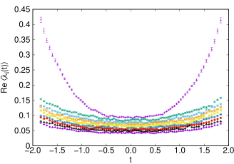
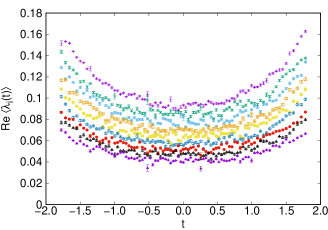
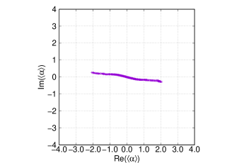
In Fig. 1, we plot the eigenvalues of the matrix (Left) and the eigenvalues of (Right). The eigenvalues are distributed on a curve which is almost parallel to the real axis for large , indicating the emergence of real time at late times333We have also confirmed that the quantity with the spatial matrices defined by (6) is close to real, indicating the emergence of real space at late times. This applies to all the cases discussed in this paper.. We also see that one out of nine eigenvalues of grows with , which suggests the emergence of an expanding (1+1)–dimensional spacetime at late times for the chosen parameters.

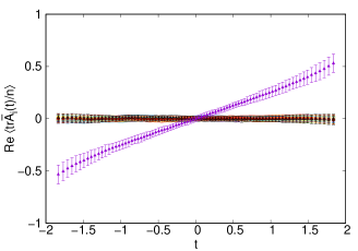
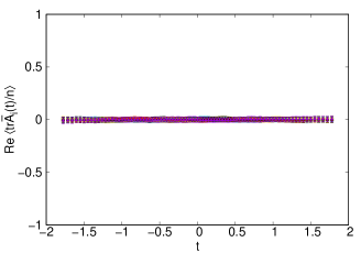
However, this is an artifact of Lorentz boosts as we see below. In Fig. 2 (Left), we plot the trace of each spatial block matrix in the SO(9) basis which diagonalizes the moment of inertia tensor . We find that one of them grows linearly in time, which indicates that the obtained configurations are Lorentz boosted. Therefore, we need to remove the effects of the Lorentz boost to obtain the proper information of the emergent spacetime.
For that purpose, we choose a Lorentz frame by minimizing the quantity
| (8) |
with respect to Lorentz transformations on each sampled configuration. This can be achieved by performing the (1+1)–dimensional Lorentz transformation
| (9) |
iteratively in such a way that the quantity (8) is minimized with respect to at each step, where and is a real parameter.
Let us discuss how is determined at each step. Plugging in Eq. (8), we get
| (10) |
Thus the problem reduces to the minimization of
| (11) |
where we have defined and
| (12) |
We find that the minimum is obtained at , where as one can prove from the inequality
| (13) |
Note that the matrix is no longer diagonal after the Lorentz transformation. Therefore, we redefine by diagonalizing as
| (14) |
where is a general complex matrix and is a complex diagonal matrix with the ordering
| (15) |
Accordingly, we transform the spatial matrices as
| (16) |
In Fig. 2 (Right), we plot the trace of each spatial matrix after the Lorentz transformation. By comparing this plot with Fig. 2 (Left), we find that the linear growth of the trace of the block matrices has disappeared.
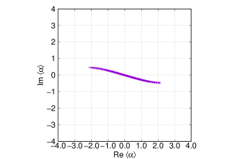
In Fig. 3, we plot the eigenvalues of the matrix (Left) and the eigenvalues of (Right) after the Lorentz transformation, which should be compared with Fig. 1. While the eigenvalue distribution of is not affected significantly by the Lorentz transformation, the nine eigenvalues of come quite close to each other after the Lorentz transformation, indicating that the 1–dimensional expansion is indeed an artifact of the Lorentz boost.
4 The effect of SUSY

When we include the fermionic contribution, the existence of near–zero eigenvalues of the Dirac operator makes the complex Langevin simulations untrustable. This problem is known as the singular drift problem [41, 42]. In order to overcome this problem, we add a fermionic mass term
| (17) |
where is a mass parameter. We eventually need to make the extrapolation to retrieve the original model. Note that, at , the fermionic degrees of freedom decouple and the model becomes equivalent to the bosonic model.
We find that the complex Langevin method works only for with the present matrix size . The results for , however, are still qualitatively the same as those of the bosonic model. In order to enhance the effect of SUSY without decreasing , we attempt to suppress the bosonic fluctuations by modifying the Lorentz invariant mass term as
| (18) |
where is an additional parameter, which is introduced to suppress the fluctuations of bosonic matrices. Note that this term breaks the Lorentz symmetry444The idea of introducing a mass term of this kind is inspired by a BMN–type deformation [43] of the type IIB matrix model, which preserves SUSY [44]. See also Ref. [45] for complex Langevin simulations of the Euclidean model with this SUSY deformation. from SO(9,1) to SO(,1) for . We show our results for this modified model with , , , and after the Lorentz transformation that removes the artifact of the Lorentz boost.
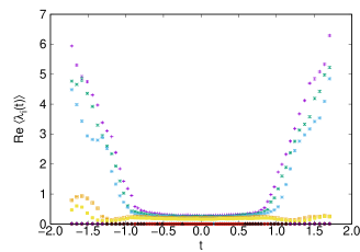
In Fig. 4, we plot the quantity defined in (3), where we see a band–diagonal structure of the spatial matrices. In Fig. 5 (Left), we plot the eigenvalues of . We find that the distribution of the eigenvalues becomes parallel to the real axis at late times, which implies that the time becomes real in that region. In Fig. 5 (Right), we plot the eigenvalues of . While the SO() spatial rotational symmetry seems to be preserved at early times, it is broken spontaneously to SO(3) at some point in time. After this SSB, only three eigenvalues start to grow. This result suggests that the expanding (3+1)–dimensional spacetime appears at late times in the presence of SUSY.
5 Summary
We have performed first–principle calculations of the Lorentzian type IIB matrix model using the Lorentz invariant mass term as an IR regulator. From the simulation of the bosonic model, we found that the Lorentz boosts may cause severe artifacts in the emergent spacetime structure. We performed a Lorentz transformation on the sampled configurations to remove these artifacts. We then found that the SSB of SO(9) does not occur in the bosonic model. Hence, the fermionic contribution is expected to be crucial for the emergence of (3+1)–dimensional spacetime.
When we include the fermionic contribution, we have to modify the model by adding the fermionic mass term (17) in order to make the complex Langevin method work. We find that, at , which is the minimal value that we were able to achieve for the present matrix size , the results are qualitatively the same as those of the bosonic model.
In order to enhance the effect of SUSY without decreasing further, we reduced the quantum fluctuations of the bosonic matrices by modifying the Lorentz invariant mass term as in Eq. (18) with the parameter . We performed simulations in the case and found that the SO() spatial rotational symmetry is spontaneously broken, and (3+1)–dimensional expanding spacetime appears at some point in time. Note that these results are obtained after the Lorentz transformation that removes the artifact of the Lorentz boosts. Recently it has been proposed [46] that the Lorentz symmetry should be "gauge–fixed" in defining the Lorentzian type IIB matrix model. Then the configurations will not get Lorentz boosted during the simulation.
In order to investigate whether the (3+1)–dimensional spacetime emerges in the original model, we need to take the limits of , , and , eventually. Performing these extrapolations is an important future direction.
Acknowledgements
T. A., K. H. and A. T. were supported in part by Grant-in-Aid (Nos.17K05425, 19J10002, and 18K03614, 21K03532, respectively) from Japan Society for the Promotion of Science. This research was supported by MEXT as “Program for Promoting Researches on the Supercomputer Fugaku” (Simulation for basic science: approaching the new quantum era, JPMXP1020230411) and JICFuS. This work used computational resources of supercomputer Fugaku provided by the RIKEN Center for Computational Science (Project IDs: hp210165, hp220174, hp230207), and Oakbridge-CX provided by the University of Tokyo (Project IDs: hp200106, hp200130, hp210094, hp220074, hp230149), and Grand Chariot provided by Hokkaido University (Project ID: hp230149) through the HPCI System Research Project. Numerical computations were also carried out on Yukawa-21 at YITP in Kyoto University and on PC clusters in KEK Computing Research Center. This work was also supported by computational time granted by the Greek Research and Technology Network (GRNET) in the National HPC facility ARIS, under the project IDs LIIB and LIIB2.
References
- [1] N. Ishibashi, H. Kawai, Y. Kitazawa, and A. Tsuchiya, “A Large N reduced model as superstring,” Nucl. Phys. B 498 (1997) 467–491, arXiv:hep-th/9612115.
- [2] J. Nishimura and F. Sugino, “Dynamical generation of four-dimensional space-time in the IIB matrix model,” JHEP 05 (2002) 001, arXiv:hep-th/0111102.
- [3] H. Kawai, S. Kawamoto, T. Kuroki, T. Matsuo, and S. Shinohara, “Mean field approximation of IIB matrix model and emergence of four-dimensional space-time,” Nucl. Phys. B 647 (2002) 153–189, arXiv:hep-th/0204240.
- [4] T. Aoyama and H. Kawai, “Higher order terms of improved mean field approximation for IIB matrix model and emergence of four-dimensional space-time,” Prog. Theor. Phys. 116 (2006) 405–415, arXiv:hep-th/0603146.
- [5] J. Nishimura, T. Okubo, and F. Sugino, “Systematic study of the SO(10) symmetry breaking vacua in the matrix model for type IIB superstrings,” JHEP 10 (2011) 135, arXiv:1108.1293 [hep-th].
- [6] K. N. Anagnostopoulos, T. Azuma, Y. Ito, J. Nishimura, and S. K. Papadoudis, “Complex Langevin analysis of the spontaneous symmetry breaking in dimensionally reduced super Yang-Mills models,” JHEP 02 (2018) 151, arXiv:1712.07562 [hep-lat].
- [7] K. N. Anagnostopoulos, T. Azuma, Y. Ito, J. Nishimura, T. Okubo, and S. Kovalkov Papadoudis, “Complex Langevin analysis of the spontaneous breaking of 10D rotational symmetry in the Euclidean IKKT matrix model,” JHEP 06 (2020) 069, arXiv:2002.07410 [hep-th].
- [8] S.-W. Kim, J. Nishimura, and A. Tsuchiya, “Expanding (3+1)-dimensional universe from a Lorentzian matrix model for superstring theory in (9+1)-dimensions,” Phys. Rev. Lett. 108 (2012) 011601, arXiv:1108.1540 [hep-th].
- [9] Y. Ito, S.-W. Kim, Y. Koizuka, J. Nishimura, and A. Tsuchiya, “A renormalization group method for studying the early universe in the Lorentzian IIB matrix model,” PTEP 2014 no. 8, (2014) 083B01, arXiv:1312.5415 [hep-th].
- [10] Y. Ito, J. Nishimura, and A. Tsuchiya, “Power-law expansion of the Universe from the bosonic Lorentzian type IIB matrix model,” JHEP 11 (2015) 070, arXiv:1506.04795 [hep-th].
- [11] T. Aoki, M. Hirasawa, Y. Ito, J. Nishimura, and A. Tsuchiya, “On the structure of the emergent 3d expanding space in the Lorentzian type IIB matrix model,” PTEP 2019 no. 9, (2019) 093B03, arXiv:1904.05914 [hep-th].
- [12] G. Parisi, “ON COMPLEX PROBABILITIES,” Phys. Lett. B 131 (1983) 393–395.
- [13] J. R. Klauder, “Coherent State Langevin Equations for Canonical Quantum Systems With Applications to the Quantized Hall Effect,” Phys. Rev. A 29 (1984) 2036–2047.
- [14] J. Nishimura and A. Tsuchiya, “Complex Langevin analysis of the space-time structure in the Lorentzian type IIB matrix model,” JHEP 06 (2019) 077, arXiv:1904.05919 [hep-th].
- [15] M. Hirasawa, K. Anagnostopoulos, T. Azuma, K. Hatakeyama, Y. Ito, J. Nishimura, S. Papadoudis, and A. Tsuchiya, “A new phase in the Lorentzian type IIB matrix model and the emergence of continuous space-time,” PoS LATTICE2021 (2022) 428, arXiv:2112.15390 [hep-lat].
- [16] K. Hatakeyama, K. Anagnostopoulos, T. Azuma, M. Hirasawa, Y. Ito, J. Nishimura, S. Papadoudis, and A. Tsuchiya, “Relationship between the Euclidean and Lorentzian versions of the type IIB matrix model,” PoS LATTICE2021 (2022) 341, arXiv:2112.15368 [hep-lat].
- [17] K. Hatakeyama, K. Anagnostopoulos, T. Azuma, M. Hirasawa, Y. Ito, J. Nishimura, S. Papadoudis, and A. Tsuchiya, “Complex Langevin studies of the emergent space-time in the type IIB matrix model,” Proceedings of the East Asia Joint Symposium on Fields and Strings 2021 (1, 2022) 9–18, arXiv:2201.13200 [hep-th].
- [18] J. Nishimura, “Signature change of the emergent space-time in the IKKT matrix model,” PoS CORFU2021 (2022) 255, arXiv:2205.04726 [hep-th].
- [19] M. Hirasawa, K. N. Anagnostopoulos, T. Azuma, K. Hatakeyama, J. Nishimura, S. K. Papadoudis, and A. Tsuchiya, “The emergence of expanding space-time in a novel large- limit of the Lorentzian type IIB matrix model,” PoS LATTICE2022 (2023) 371, arXiv:2212.10127 [hep-lat].
- [20] M. Hirasawa, K. N. Anagnostopoulos, T. Azuma, K. Hatakeyama, J. Nishimura, S. Papadoudis, and A. Tsuchiya, “The emergence of expanding space-time in the Lorentzian type IIB matrix model with a novel regularization,” PoS CORFU2022 (2023) 309, arXiv:2307.01681 [hep-th].
- [21] K. N. Anagnostopoulos, T. Azuma, K. Hatakeyama, M. Hirasawa, Y. Ito, J. Nishimura, S. K. Papadoudis, and A. Tsuchiya, “Progress in the numerical studies of the type IIB matrix model,” Eur. Phys. J. ST 232 no. 23-24, (2023) 3681–3695, arXiv:2210.17537 [hep-th].
- [22] S. Brahma, R. Brandenberger, and S. Laliberte, “BFSS Matrix Model Cosmology: Progress and Challenges,” arXiv:2210.07288 [hep-th].
- [23] F. R. Klinkhamer, “Emergent gravity from the IIB matrix model and cancellation of a cosmological constant,” Class. Quant. Grav. 40 no. 12, (2023) 124001, arXiv:2212.00709 [hep-th].
- [24] H. C. Steinacker, Quantum Geometry, Matrix Theory, and Gravity. Cambridge University Press, 4, 2024.
- [25] H. C. Steinacker, “Cosmological space-times with resolved Big Bang in Yang-Mills matrix models,” JHEP 02 (2018) 033, arXiv:1709.10480 [hep-th].
- [26] H. C. Steinacker, “Quantized open FRW cosmology from Yang–Mills matrix models,” Phys. Lett. B 782 (2018) 176–180, arXiv:1710.11495 [hep-th].
- [27] M. Sperling and H. C. Steinacker, “The fuzzy 4-hyperboloid and higher-spin in Yang–Mills matrix models,” Nucl. Phys. B 941 (2019) 680–743, arXiv:1806.05907 [hep-th].
- [28] M. Sperling and H. C. Steinacker, “Covariant cosmological quantum space-time, higher-spin and gravity in the IKKT matrix model,” JHEP 07 (2019) 010, arXiv:1901.03522 [hep-th].
- [29] H. C. Steinacker, “Scalar modes and the linearized Schwarzschild solution on a quantized FLRW space-time in Yang–Mills matrix models,” Class. Quant. Grav. 36 no. 20, (2019) 205005, arXiv:1905.07255 [hep-th].
- [30] H. C. Steinacker, “Higher-spin kinematics & no ghosts on quantum space-time in Yang–Mills matrix models,” Adv. Theor. Math. Phys. 25 no. 4, (2021) 1025–1093, arXiv:1910.00839 [hep-th].
- [31] H. C. Steinacker, “On the quantum structure of space-time, gravity, and higher spin in matrix models,” Class. Quant. Grav. 37 no. 11, (2020) 113001, arXiv:1911.03162 [hep-th].
- [32] K. Hatakeyama, A. Matsumoto, J. Nishimura, A. Tsuchiya, and A. Yosprakob, “The emergence of expanding space–time and intersecting D-branes from classical solutions in the Lorentzian type IIB matrix model,” PTEP 2020 no. 4, (2020) 043B10, arXiv:1911.08132 [hep-th].
- [33] H. C. Steinacker, “Higher-spin gravity and torsion on quantized space-time in matrix models,” JHEP 04 (2020) 111, arXiv:2002.02742 [hep-th].
- [34] S. Fredenhagen and H. C. Steinacker, “Exploring the gravity sector of emergent higher-spin gravity: effective action and a solution,” JHEP 05 (2021) 183, arXiv:2101.07297 [hep-th].
- [35] H. C. Steinacker, “Gravity as a quantum effect on quantum space-time,” Phys. Lett. B 827 (2022) 136946, arXiv:2110.03936 [hep-th].
- [36] Y. Asano and H. C. Steinacker, “Spherically symmetric solutions of higher-spin gravity in the IKKT matrix model,” Nucl. Phys. B 980 (2022) 115843, arXiv:2112.08204 [hep-th].
- [37] J. L. Karczmarek and H. C. Steinacker, “Cosmic time evolution and propagator from a Yang–Mills matrix model,” J. Phys. A 56 no. 17, (2023) 175401, arXiv:2207.00399 [hep-th].
- [38] E. Battista and H. C. Steinacker, “On the propagation across the big bounce in an open quantum FLRW cosmology,” Eur. Phys. J. C 82 no. 10, (2022) 909, arXiv:2207.01295 [gr-qc].
- [39] F. Attanasio and B. Jäger, “Dynamical stabilisation of complex Langevin simulations of QCD,” Eur. Phys. J. C 79 no. 1, (2019) 16, arXiv:1808.04400 [hep-lat].
- [40] M. W. Hansen and D. Sexty, “Testing dynamical stabilization of Complex Langevin simulations of QCD,” arXiv:2405.20709 [hep-lat].
- [41] J. Nishimura and S. Shimasaki, “New insights into the problem with a singular drift term in the complex Langevin method,” Phys. Rev. D92 no. 1, (2015) 011501, arXiv:1504.08359 [hep-lat].
- [42] K. Nagata, J. Nishimura, and S. Shimasaki, “Argument for justification of the complex Langevin method and the condition for correct convergence,” Phys. Rev. D 94 no. 11, (2016) 114515, arXiv:1606.07627 [hep-lat].
- [43] D. E. Berenstein, J. M. Maldacena, and H. S. Nastase, “Strings in flat space and pp waves from N=4 superYang-Mills,” JHEP 04 (2002) 013, arXiv:hep-th/0202021.
- [44] G. Bonelli, “Matrix strings in pp wave backgrounds from deformed superYang-Mills theory,” JHEP 08 (2002) 022, arXiv:hep-th/0205213.
- [45] A. Kumar, A. Joseph, and P. Kumar, “Investigating Spontaneous SO(10) Symmetry Breaking in Type IIB Matrix Model,” in 25th DAE-BRNS High Energy Physics Symposium. 8, 2023. arXiv:2308.03607 [hep-lat].
- [46] Y. Asano, J. Nishimura, W. Piensuk, and N. Yamamori, “Defining the type IIB matrix model without breaking Lorentz symmetry,” arXiv:2404.14045 [hep-th].