Construct accurate multi-continuum micromorphic homogenisations in multi-D space-time with computer algebra

Abstract

Homogenisation empowers the efficient macroscale system level prediction of physical problems with intricate microscale structures. Here we develop an innovative powerful, rigorous and flexible framework for asymptotic homogenisation of dynamics at the finite scale separation of real physics, with proven results underpinned by modern dynamical systems theory. The novel systematic approach removes most of the usual assumptions, whether implicit or explicit, of other methodologies. By no longer assuming averages the methodology constructs so-called multi-continuum or micromorphic homogenisations systematically based upon the microscale physics. The developed framework and approach enables a user to straightforwardly choose and create such homogenisations with clear physical and theoretical support, and of highly controllable accuracy and fidelity.

1 Introduction

In most standard constitutive models for the mechanical behaviour of solids, the stress at a given point uniquely depends on the current deformation gradients (e.g., Bažant & Jirásek 2002). However, modern designed metamaterials have exceptional mechanical properties that depend largely on the intricate underlying complicated microstructure, rather than the bulk properties of their constituent materials (e.g., Sarhil et al. 2024). So-called multi-continuum or micromorphic homogenisations, or generalized Cosserat theories, are enhanced models which aim to capture the significant macroscale effects of such heterogenous microstructure without fully-resolving the microstructures (e.g., Alavi et al. 2023). fig. 1 shows one example of a microstructured material whose macroscale deformation can only adequately be predicted by the generalised modelling of non-standard microscale modes Rokoš et al. (2019). The pioneering vision of Muncaster (1983a) was that the dynamical systmes concept of invariant manifolds would provide a general rigorous route to coarse-scale modelling of nonlinear dynamics in mechanics. Here we develop a flexible, systematic and practical approach to the multi-continuum homogenisation modelling of heterogeneous systems (such as the material deformation of fig. 1) using modern developments in the rigorous theory and application of invariant manifolds for nonlinear dynamical systems Aulbach & Wanner (2000), Potzsche & Rasmussen (2006), Haragus & Iooss (2011), Roberts (2015a), Bunder & Roberts (2021).

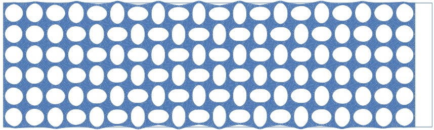
Figure 1: 4% compression of a material with circular inclusions, seen near either end, may develop a nontrivial microscale structure, seen near the middle (from Figure 4(2nd) of Guo et al. (2024)). Macroscale homogenisation of such microscale structures may best be via a multi-continuum model.

This article greatly extends a novel dynamical systems approach Bunder & Roberts (2021) to multi-continua/micromorphic homogenisation in two major parts. The first part, sections 2, 3 and 4, introduce the key ideas and methods in the more accessible scenario of the linear self-adjoint dynamics of a scalar field in space-time with one large spatial dimension and microscale periodic heterogenity. The second part, sections 5 and 6, develops the framework and theory of the methodology, and an application, to a wide class of nonlinear non-autonomous dynamics of a general field in space-time with arbitrary number of ‘large spatial’ dimensions and heterogeneity on both the macroscale and quasi-periodic microscale. For an example in 2-D elasticity: section 6.4.2 derives a homogenisation in terms of high-order gradients of the usual two mean displacements; whereas section 6.4.3 derives a tri-continuum homogenisation in three degrees of freedom as determined by the sub-cell physics of the heterogeneous elasticity.

Three broad families of methods enhance standard homogenisation (e.g., Bažant & Jirásek 2002, Forest & Trinh 2011, Sarhil et al. 2024): firstly, introduce extra fields, the multi-continua, that provide supplementary information on the small-scale kinematics; secondly, improve the resolution of the standard displacement-field modelling by incorporating higher-order gradients; and thirdly, introduce nonlocal effects into the homogenisation. Our systematic dynamical systems framework and results unifies the approach and connects to all three of these families, in order: firstly, multi-continuum Cosserat-like theories are the central theme; secondly, higher-order gradient models are invoked for examples of both basic homogenisation (sections 4.2 and 6.4.2) and also multi-continua homogenisation (sections 4.3, 4.4 and 3.2); and lastly, examples of accurate nonlocal models are created by regularising some of the higher-order models (sections 4.2 and 3.2.2). Craster (2015) commented that “Homogenization theory is typically limited to static or quasi-static low frequency situations and the purpose of this contribution is to briefly review how to tackle dynamic situations” Our contribution also focusses on dynamics, with statics being the special case of no time variations.

Introduce the novel methodology

In a plenary lecture Forest & Trinh (2011) discussed that “in most cases … proposed extended homogenization procedures [for micromorphic continua] remain heuristic”. In contrast, the novel approach here is created by innovatively synthesising three separate ingredients from the mathematics of dynamical systems. Let’s summarise the three ingredients.

• Firstly, it seems paradoxical that macroscale homogenisations have translationally invariant symmetry in space, say $x$, given that the underling microscale is spatially heterogeneous in $x$. Here is that we embed the given heterogeneous problem in the family of all phase-shifted problems (sections 2.1 and 5.1). In the special embedding, the family of problems is translationally symmetric in $x$, with the heterogeneity in an orthogonal ‘thin space’ dimension. Consequently, homogenisation then preserves the embedded system’s translational symmetry in $x$.

• Secondly, the orthogonal ‘thin space’ dimension gives rise to the classic cell-problem (rve problem) with periodicity naturally required (sections 2.2 and 5.2). Then the theory of invariant manifolds supports choosing multi-continuum modes from the eigenmodes corresponding to small eigenvalues because for a wide range of circumstances one is then guaranteed the multi-continuum modelling is exponentially quickly emergent (section 5.2.2) Such multi-mode modelling in spatially extensive systems was initiated by Watt & Roberts (1995) for the shear dispersion in flow along a channel.

• Thirdly, recently Bunder & Roberts (2021) developed an invariant manifold at each spatial locale, weakly coupled to neighbouring locales, via a multivariate Taylor series in space. A new remainder term for the series (Bunder & Roberts 2021, expression (44)) quantifies the error of the modelling so that the multiscale homogenisation is valid simply wherever and whenever the remainder term is small enough for the purposes at hand.

Recently, Alavi et al. (2023) [p.2166] noted one limitation of other approaches is that “proper elaboration of the macroscopic kinematic and static quantities that pertain to the micromorphic continuum is a problematic issue … [previous] works did not relate macroscopic to microscopic kinematic quantities and they did not formulate a boundary value problem at the microscale.” In contrast, here embedding the system provides via dynamics theory a sound boundary value problem (e.g., (LABEL:Eemdifpde,Eempde)), and the constructed invariant manifolds explicitly connect the microscale to the selected macroscale kinematic quantities (e.g., (LABEL:E1d3Mman,EhcegManifold3u)).

Strong theoretical support

Alavi et al. (2023) [p.2165] also commented that “Periodic homogenization methods … are most of the time lacking a clear mathematical proof of convergence of the microscopic solution towards the limit solution for vanishing values of the scale parameter” Complementing this, in their review Fish et al. (2021) discuss that [p.775] “Mathematical homogenization theory based on the multiple-scale asymptotic expansion assumes scale separation.” Such scale separation is usually defined as the mathematical limit $\ell/L\to 0$ for microscale lengths $\ell$ and macroscale lengths $L$. Here there is no such limit assumed. Instead, using established dynamical systems theory of invariant manifolds provides such proofs in two main cases (e.g., Aulbach & Wanner 2000, Potzsche & Rasmussen 2006, Haragus & Iooss 2011, Roberts 2015a, Bunder & Roberts 2021). The first case is that of systems with some damping for which section 5.2.2 creates a framework with clear mathematical proofs of the existence of models with exact closure, with convergence in time to the macroscale model, and that is controllably approximated. The second case is that of undamped, wave-like, systems where section 5.2.3 argues that we can prove that constructed nearby systems possess exact guiding-centre macroscale homogenisations. Moreover, these proofs are not just for the vanishing scale parameter limit, but for the finite scale separations of real applications.

Alavi et al. (2023) [pp.2164–5] discussed how “generalized continuum models … face some limitations in their capability to predict microstructures’ supposedly intrinsic mechanical properties accurately.” Similarly, Fish et al. (2021) [p.776] commented that “In upscaling methods, the fine-scale response is approximated or idealized, and only its average effect is captured.” In contrast, invariant manifold theory guarantees the existence of an exact closure for multi-continuum homogenisations in some domain (section 5.2), a closure that exactly captures the fine-scale response. Importantly, our approach does not invoke assumed averaging. Further, theory Potzsche & Rasmussen (2006) guarantees we approximate the exact closure to a controllable accuracy.

Quantifying errors and uncertainty

In a broad-ranging discussion of multiscale simulation of materials, Chernatynskiy et al. (2013) [p.160] asserted that “quantifying the errors at each scale is challenging, quantifying how those errors propagate across scales is an even more daunting task” which has two aspects rectified here. Firstly, as mentioned above, our approach connects with innovative quantitive estimates for the remainder error incurred by the macroscale modelling: in the case of one large spatial dimension via expression (23) of Roberts (2015a); in the case of multiple large dimensions via expression (44) of Bunder & Roberts (2021). Secondly, the dynamical systems framework established here comes with (in future research) a systematic accurate projection of initial conditions (e.g., Roberts 1989, Watt & Roberts 1995). The same projection also rationally propagates errors and uncertainty from micro- to macro-scales. Thus error propagation no longer need be such a “daunting task”.

Clarify and guide the hierarchy of multi-continua choices

Rizzi et al. (2021) [p.2253] concluded that “It is thus an an important future task … to derive guidelines for a favorable choice among the numerous available micromorphic continuum models.” The dynamical systems approach established here clarifies and guides the choice of multi-continuum models depending upon the space-time scales the modelling needs to resolve. sections 2.2, 4.1, 5.2 and 6.4 organise choices into a sequence of possibilities, and then guides a choice in the sequence depending upon the spatio-temporal scales of interest in the envisaged scenarios of application.

Alavi et al. (2023) [p.2164] also raises the “difficulty to choose a priori an appropriate model for a given microstructure. Enriched continuum theories are required in such situations to capture the effect of spatially rapid fluctuations at the mesoscopic and macroscopic levels. … micromorphic homogenization raises specific difficulties compared to higher gradient and higher-order theories” The dynamical systems framework herein, as discussed by section 5.2.5, empowers us to also guide the selection of multi-continuum modes aimed to improve spatial resolution, irrespective of the temporal resolution.

Efendiev & Leung (2023) also use a spectral decomposition to guide multi-continuum models. However, they require macroscale variables $U_{i}$ to be averages and hence deduce [p.3] “unless there is some type of high contrast, the averages … will become similar” which leads them to conclude [p.16] that for “multi-continuum models, … one needs high contrast to have different average values”. In contrast, the approach here is not wedded to averaging, so is more flexible, and need not be limited to high contrast (although section 4 details a high contrast example, the example of section 3 is not). By measuring and being based upon whatever structures the physical equations tell us about sub-cell dynamics we here form and justify more general multi-continuum models.

Moreover, many commonly made assumptions are not needed here. There are no guessed fast/slow variables, no small $\epsilon$s, no limits, no need to assume a variational formulation, nor energy functional, nor presume specific sub-cell modes, nor need oversampling regions, nor assume boundary conditions for rves, nor assume multiple times scaled by powers of a small $\epsilon$.

Computer algebra handles complicated details

Rizzi et al. (2021) [p.2237] began by highlighting that a “basic problem of all these theories … is the huge number of newly appearing constitutive coefficients which need to be determined.” The systematic nature of our approach, together with theoretical support (e.g., Potzsche & Rasmussen 2006), empowers computer algebra to routinely handle the potentially “huge number” of constitutive coefficients via a robust and flexible algorithm introduced by Roberts (1997) and documented for many applications in a subsequent book Roberts (2015b). appendices A, B and C list adaptable code for the three major examples of sections 3, 4 and 6—the latter two integrating fine-scale numerics with the macroscale algebra. These codes specifically use the computer algebra system Reduce as it is free, flexible, and fast Fateman (2003).

Alavi et al. (2023) [p.2164] commented that “micromorphic homogenization raises specific difficulties compared to higher gradient and higher-order theories” In contrast, here we apply the same theoretical and practical framework for all cases with no difficulty, indeed with the same code via just a couple of parameter changes to change from standard to multi-continuum micromorphic homogenisations, and from leading order to any arbitrary higher-order.

Let’s proceed with the basics of the approach in 1-D space, sections 2, 3 and 4, before addressing the complexities of general nonlinear systems in multi-D space, sections 5 and 6.

2 Systematic multi-continuum homogenisation for 1-D spatial systems

The idea here is to establish and construct so-called multi-continuum or micromorphic homogenised models in 1-D space. Now a “multi-continuum” or “micromorphic” model is phrased in terms of microscale structures/modes that have macroscale variations—in essence pursuing models with multiple mode-shapes in the microscale (e.g., Rokoš et al. 2019, Alavi et al. 2023, Sarhil et al. 2024). Here we develop multi-continuum homogenisation by the novel combination of analysing the ensemble of phase-shifts Roberts (2015a) via innovations to the multi-modal dynamical systems modelling of Watt & Roberts (1995).

The distinguishing feature here is that we let the microscale physical dynamics of the system inform and determine almost all decisions. We do not assume any particular weighted averages are appropriate for variables, nor do we assume any particular weighted averages are appropriate for any upscaling dimensional reduction. The only subjective decision made herein is how many microscale modes one wishes to resolve in the multiscale modelling. This decision is strongly guided by the physics-determined spectrum of the microscale (sections 4.1 and 5.2).

Consider materials with complicated microstructure. We want to model their macroscale dynamics over a large scale $L$ by equations with effective ‘average’ coefficients, but without presuming any averaging. Heterogeneous second-order systems in 1-D space are the simplest such class of systems: suppose the material, in spatial domain $[0,L]$, has structure so that ‘material’ or ‘heat’ $u(t,x)$ evolves according to the pde

$$\mathchoice{\frac{\partial^{\alpha}u}{\partial t^{\alpha}}}{{\partial^{\alpha}u}/{\partial t^{\alpha}}}{{\partial^{\alpha}u}/{\partial t^{\alpha}}}{{\partial^{\alpha}u}/{\partial t^{\alpha}}}=\mathchoice{\frac{\partial}{\partial x}}{{\partial}/{\partial x}}{{\partial}/{\partial x}}{{\partial}/{\partial x}}\left\{\kappa(x)\mathchoice{\frac{\partial u}{\partial x}}{{\partial u}/{\partial x}}{{\partial u}/{\partial x}}{{\partial u}/{\partial x}}\right\},\quad 0<x<L\,,$$ (2.1)

where the heterogeneous material coefficient $\kappa(x)$ has some complicated microscale structure on a microscale length $\ell$, and so the solution field $u(t,x)$ has complicated multiscale structures. We assume that the coefficient $\kappa(x)$ is regular enough that there exist general solutions $u(t)$ in the Sobolev space $W^{2,2}([0,L])$.

The time evolution operator $\mathchoice{\frac{\partial^{\alpha}}{\partial t^{\alpha}}}{{\partial^{\alpha}}/{\partial t^{\alpha}}}{{\partial^{\alpha}}/{\partial t^{\alpha}}}{{\partial^{\alpha}}/{\partial t^{\alpha}}}$, usually written $\partial_{t}^{\alpha}$ herein, covers many cases: $\alpha=1$ is a prototypical diffusion problem; $\alpha=2$ is a prototypical wave problem; fractional $\alpha$ could represent the fractional calculus operator; but potentially $\partial_{t}^{\alpha}$ could represent any in a wide variety of time evolution operators that commutes with spatial derivatives, such as the time-step operator $\partial_{t}^{\alpha}u\mapsto(u|_{t}-u|_{t-\tau})/\tau$. We primarily discuss the two main cases of diffusive-like dynamics and of wave-like dynamics, $\alpha=1,2$ respectively.

Our approach provides a homogenisation at finite scale separation $\ell/L$ of real scenarios, we do not take the limit $\ell/L\to 0$. The approach is informed by the emergent physics arising from the microscale interactions. However, we require that the length $L$ is sufficiently large that we can focus on modelling interesting dynamics in the interior of the domain, say the open set ${\mathbb{X}}\subset[0,L]$, significantly away from the boundaries at $x=0,L$ and the associated boundary layers. A systematic and accurate homogenisation modelling of physical boundaries and associated boundary layers in multiscale homogenisation is a topic for future research (perhaps via the approach of Roberts 1992, Chen et al. 2018).

For the multiscale pde eq. 2.1, and in the diffusive case $\alpha=1$, Roberts (2024) derived, supported, and characterised the one-mode macroscale homogenised pde

$$\partial_{t}^{\alpha}U=KU_{xx}+\cdots\,,\quad\text{for }x\in{\mathbb{X}}\,,$$ (2.2)

for some effective mean field $U(t,x)$, some macroscale effective material constant $K$, with some higher order corrections denoted by the ellipsis $\cdots$, and a potentially quantified error estimate (via (23) of Roberts 2015a). Instead of the one-mode model eq. 2.2, the task here is to argue for, theoretically support, and construct, a multi-continuum, micromorphic, multi-modal homogenisation model. The main aim for such a multi-continuum homogenisation is to improve the space-time resolution over that of (2.2).

For an example, section 3 develops a three-mode, tri-continuum, homogenisation expressed in terms of three macroscale quantities $U_{0},U_{1},U_{2}$, defined by the microscale physics, that evolve within $\mathbb{X}$ according to the three macroscale pdes

$$\partial_{t}^{\alpha}U_{0}=kU_{0xx}-\tfrac{1}{2}aU_{1x}+\cdots, \partial_{t}^{\alpha}U_{1}=-U_{1}+aU_{0x}+\cdots,$$

$$\partial_{t}^{\alpha}U_{2}=-U_{2}+2U_{1x}+\cdots.$$ (2.3)

Because our sound modelling is transitive, the classic homogenised one-mode pde eq. 2.2 may be recovered by the adiabatic quasi-equilibrium approximation of the second mode in eq. 2.3: this adiabatic approximation gives $U_{1}\approx aU_{0x}$. Consequently, the first pde of eq. 2.3 reduces to the usual homogenised macroscale pde $\partial_{t}^{\alpha}U_{0}\approx(k-\tfrac{1}{2}a^{2})U_{0xx}$ .

Generalisations to any number of multi-continuum modes are straightforward, as coded in the computer algebra of appendices A and B for the respective examples of sections 3 and 4.

Fish et al. (2021) [p.774] identified that a challenge for “a multiscale approach involves a trade-off between increased model fidelity with the added complexity, and corresponding reduction in precision and increase in uncertainty”. Here there is no trade-off with increased fidelity: both here and in section 5 we establish a framework with proven controllable precision and certainty.

The theoretical support for multi-continuum models such as eq. 2.3 depends upon the time evolution operator $\partial_{t}^{\alpha}$. For the attributes of existence and construction, for general $\partial_{t}^{\alpha}$ it appears best to appeal to a version of backwards theory Roberts (2022), Hochs & Roberts (2019), namely that the constructed invariant manifold and homogenised evolution eq. 2.3 thereon is exact for a system close to the specified multiscale pde eq. 2.1. The major practical difference among the various $\partial_{t}^{\alpha}$ is whether the dimension-reduced, approximate invariant manifold, multi-modal models such as eq. 2.3 are emergent in time: for diffusion, $\alpha=1$, the homogenised models are generally exponentially quickly emergent in time; for elastic waves, $\alpha=2$, the homogenised models are best viewed as a guiding centre for the dynamics about the constructed manifold (e.g., van Kampen 1985); whereas for other cases the relevance of the modelling depends upon how the spectrum of the right-hand side operator of eq. 2.1 maps into dynamics of the corresponding modes. section 5.2 discusses these cases in more detail.

Of course, if one only addresses forced equilibrium problems, or Helmholtz-like equations for a specified frequency, then the issue of whether the modelling is relevant under time evolution need not be considered.

2.1 Phase-shift embedding

Our powerful innovative alternative approach to homogenisation is to embed the specific given physical pde (2.1) into a family of pde problems formed by all phase-shifts of the periodic microscale Roberts (2015a). This embedding is a novel and rigorous twist to the concept of a Representative Volume Element.

Let’s create the desired embedding for pdes (2.1) in 1-D space by considering a field ${\mathfrak{u}}(t,{{\cal\mathchoice{\scriptstyle X}{\scriptstyle X}{\scriptscriptstyle X}{\scriptscriptstyle X}}},\theta)$ satisfying the pde

$$\mathchoice{\frac{\partial^{\alpha}{\mathfrak{u}}}{\partial t^{\alpha}}}{{\partial^{\alpha}{\mathfrak{u}}}/{\partial t^{\alpha}}}{{\partial^{\alpha}{\mathfrak{u}}}/{\partial t^{\alpha}}}{{\partial^{\alpha}{\mathfrak{u}}}/{\partial t^{\alpha}}}=\left(\mathchoice{\frac{\partial}{\partial{{\cal\mathchoice{\scriptstyle X}{\scriptstyle X}{\scriptscriptstyle X}{\scriptscriptstyle X}}}}}{{\partial}/{\partial{{\cal\mathchoice{\scriptstyle X}{\scriptstyle X}{\scriptscriptstyle X}{\scriptscriptstyle X}}}}}{{\partial}/{\partial{{\cal\mathchoice{\scriptstyle X}{\scriptstyle X}{\scriptscriptstyle X}{\scriptscriptstyle X}}}}}{{\partial}/{\partial{{\cal\mathchoice{\scriptstyle X}{\scriptstyle X}{\scriptscriptstyle X}{\scriptscriptstyle X}}}}}+\mathchoice{\frac{\partial}{\partial\theta}}{{\partial}/{\partial\theta}}{{\partial}/{\partial\theta}}{{\partial}/{\partial\theta}}\right)\left\{\kappa(\theta)\left(\mathchoice{\frac{\partial{\mathfrak{u}}}{\partial{{\cal\mathchoice{\scriptstyle X}{\scriptstyle X}{\scriptscriptstyle X}{\scriptscriptstyle X}}}}}{{\partial{\mathfrak{u}}}/{\partial{{\cal\mathchoice{\scriptstyle X}{\scriptstyle X}{\scriptscriptstyle X}{\scriptscriptstyle X}}}}}{{\partial{\mathfrak{u}}}/{\partial{{\cal\mathchoice{\scriptstyle X}{\scriptstyle X}{\scriptscriptstyle X}{\scriptscriptstyle X}}}}}{{\partial{\mathfrak{u}}}/{\partial{{\cal\mathchoice{\scriptstyle X}{\scriptstyle X}{\scriptscriptstyle X}{\scriptscriptstyle X}}}}}+\mathchoice{\frac{\partial{\mathfrak{u}}}{\partial\theta}}{{\partial{\mathfrak{u}}}/{\partial\theta}}{{\partial{\mathfrak{u}}}/{\partial\theta}}{{\partial{\mathfrak{u}}}/{\partial\theta}}\right)\right\},\quad{\mathfrak{u}}\text{ $\ell$-periodic in }\theta,$$ (2.4)

in the ‘cylindrical’ domain ${\mathbb{D}}:=\{({{\cal\mathchoice{\scriptstyle X}{\scriptstyle X}{\scriptscriptstyle X}{\scriptscriptstyle X}}},\theta):{{\cal\mathchoice{\scriptstyle X}{\scriptstyle X}{\scriptscriptstyle X}{\scriptscriptstyle X}}}\in{\mathbb{X}}\mathchar 8507\relax{}\theta\in\Theta:=[0,\ell]\}$. We assume the lower bound $\kappa(\theta)\geq\kappa_{\min}>0$, and that the heterogeneity $\kappa(\theta)$ is regular enough that general solutions $\mathfrak{u}$ of pde eq. 2.4 are in ${\mathbb{H}}^{N}_{\mathbb{D}}:=W^{(N+1,2),2}({\mathbb{D}})$ for some chosen order $N$, and where we define the Sobolev space $W^{{\text{\boldmath$q$}},p}({\mathbb{D}}):=\{u\in L^{p}({\mathbb{D}}):\partial_{{\cal\mathchoice{\scriptstyle X}{\scriptstyle X}{\scriptscriptstyle X}{\scriptscriptstyle X}}}^{a_{1}}\partial_{\theta}^{a_{2}}u\in L^{p}({\mathbb{D}})\mathchar 8507\relax{}a_{i}\leq q_{i}\}$. For example, choose $N=2$ for the classic eq. 2.2 or tri-continuum eq. 2.3 homogenisations, or choose $N\geq 4$ for higher-order homogenisations (e.g., sections 3.2, 4.3 and 6.4.2). I emphasise that the domain ${\mathbb{D}}$ of pde eq. 2.4 has finite aspect ratio: we do not take the usual scale-separation limit involving an aspect ratio tending to zero nor to infinity.

Lemma 1.

For every solution ${\mathfrak{u}}(t,{{\cal\mathchoice{\scriptstyle X}{\scriptstyle X}{\scriptscriptstyle X}{\scriptscriptstyle X}}},\theta)\in{\mathbb{H}}^{N}_{\mathbb{D}}$ of the embedding pde (2.4), and for every phase $\phi$, the defined field $u_{\phi}(t,x):={\mathfrak{u}}(t,x,x+\phi)$ is in the Sobolov space ${\mathbb{H}}^{2}_{\mathbb{X}}:=W^{2,2}({\mathbb{X}})$ and satisfies the heterogeneous diffusion pde

$$\mathchoice{\frac{\partial^{\alpha}u_{\phi}}{\partial t^{\alpha}}}{{\partial^{\alpha}u_{\phi}}/{\partial t^{\alpha}}}{{\partial^{\alpha}u_{\phi}}/{\partial t^{\alpha}}}{{\partial^{\alpha}u_{\phi}}/{\partial t^{\alpha}}}=\mathchoice{\frac{\partial}{\partial x}}{{\partial}/{\partial x}}{{\partial}/{\partial x}}{{\partial}/{\partial x}}\left\{\kappa(x+\phi)\mathchoice{\frac{\partial u_{\phi}}{\partial x}}{{\partial u_{\phi}}/{\partial x}}{{\partial u_{\phi}}/{\partial x}}{{\partial u_{\phi}}/{\partial x}}\right\}.$$ (2.5)

Specifically, for the case of phase $\phi=0$, the field $u(t,x):=u_{0}(t,x)={\mathfrak{u}}(t,x,x)$ satisfies the given heterogeneous pde (2.1).

Note the implicit distinction among $x$-derivatives: $\mathchoice{\frac{\partial}{\partial{{\cal\mathchoice{\scriptstyle X}{\scriptstyle X}{\scriptscriptstyle X}{\scriptscriptstyle X}}}}}{{\partial}/{\partial{{\cal\mathchoice{\scriptstyle X}{\scriptstyle X}{\scriptscriptstyle X}{\scriptscriptstyle X}}}}}{{\partial}/{\partial{{\cal\mathchoice{\scriptstyle X}{\scriptstyle X}{\scriptscriptstyle X}{\scriptscriptstyle X}}}}}{{\partial}/{\partial{{\cal\mathchoice{\scriptstyle X}{\scriptstyle X}{\scriptscriptstyle X}{\scriptscriptstyle X}}}}}$ of $\mathfrak{u}$ is done keeping $\theta$ constant; whereas $\mathchoice{\frac{\partial}{\partial x}}{{\partial}/{\partial x}}{{\partial}/{\partial x}}{{\partial}/{\partial x}}$ of $u$ and $u_{\phi}$ is done keeping phase $\phi$ constant.

Proof.

The proofs for sections 2.1 and 2.1 are straightforward, and are encompassed by the proofs given for sections 5.1 and 5.1. ∎

Here the microscale $\ell$-periodic boundary conditions are not assumed but arise naturally due to the ensemble of phase-shifts. That is, what previously had to be assumed, here arises naturally.

Lemma 2 (converse).

Suppose we have a set of solutions $u_{\phi}(t,x)$ of the phase-shifted pde (2.5)—a set parametrised by the phase vector $\phi$—and the set depends smoothly enough upon $t,x,\phi$ that the following ${\mathfrak{u}}\in{\mathbb{H}}^{N}_{\mathbb{D}}$. Then the field ${\mathfrak{u}}(t,{{\cal\mathchoice{\scriptstyle X}{\scriptstyle X}{\scriptscriptstyle X}{\scriptscriptstyle X}}},\theta):=u_{\theta-{{\cal\mathchoice{\scriptstyle X}{\scriptstyle X}{\scriptscriptstyle X}{\scriptscriptstyle X}}}}(t,{{\cal\mathchoice{\scriptstyle X}{\scriptstyle X}{\scriptscriptstyle X}{\scriptscriptstyle X}}})$ satisfies the embedding pde (2.4).

Consequently, pdes (LABEL:Eemdifpde,Eshdifpde) are equivalent, and they may provide us with a set of solutions for an ensemble of materials all with the same heterogeneity structure, but with the structural phase of the material shifted through all possibilities. The critical difference between the pdes eqs. 2.1 and 2.5 and the embedding pde eq. 2.4 is that although pdes (LABEL:Ehdifpde,Eshdifpde) are heterogeneous in space $x$, the embedding pde (2.4) is homogeneous in ${{\cal\mathchoice{\scriptstyle X}{\scriptstyle X}{\scriptscriptstyle X}{\scriptscriptstyle X}}}$.

2.2 Invariant manifolds of multi-modal any-order homogenization

We now analyse the embedding pde (2.4) for useful invariant manifolds via an approach proven for systems homogeneous in the long space, $x$-direction. The invariant manifolds express and support the relevance of a precise multi-modal homogenization of the original heterogeneous pde (2.1). Since the pdes herein are linear, the invariant manifolds are more specifically invariant subspaces, but let’s use the term manifold as the same framework and theory immediately generalises to related nonlinear systems as discussed in section 5.

Rigorous theory (Roberts 2015a) inspired by earlier more formal arguments (Roberts 1988, 1997) establishes how to support and construct pde models for the macroscale spatial structure of pde solutions in cylindrical domains such as $\mathbb{D}$. The technique is to base analysis on the case where variations in $x$ are approximately negligible, and then treat slow, macroscale, variations in $x$ as a regular perturbation (Roberts 2015b, Part III).

To establish the basis of an invariant manifold, consider the embedding pde (2.4) with $\mathchoice{\frac{\partial}{\partial x}}{{\partial}/{\partial x}}{{\partial}/{\partial x}}{{\partial}/{\partial x}}$ neglected:

$$\mathchoice{\frac{\partial^{\alpha}{\mathfrak{u}}}{\partial t^{\alpha}}}{{\partial^{\alpha}{\mathfrak{u}}}/{\partial t^{\alpha}}}{{\partial^{\alpha}{\mathfrak{u}}}/{\partial t^{\alpha}}}{{\partial^{\alpha}{\mathfrak{u}}}/{\partial t^{\alpha}}}=\mathchoice{\frac{\partial}{\partial\theta}}{{\partial}/{\partial\theta}}{{\partial}/{\partial\theta}}{{\partial}/{\partial\theta}}\left\{\kappa(\theta)\left(\mathchoice{\frac{\partial{\mathfrak{u}}}{\partial\theta}}{{\partial{\mathfrak{u}}}/{\partial\theta}}{{\partial{\mathfrak{u}}}/{\partial\theta}}{{\partial{\mathfrak{u}}}/{\partial\theta}}\right)\right\},\quad{\mathfrak{u}}\text{ is $\ell$-periodic in }\theta.$$ (2.6)

The basis obtained here applies in a locale around each and every $x\in{\mathbb{X}}$ (Roberts 2015a, §2). In general, as in some functionally graded materials and as addressed in section 5, the details of such a basis varies with locale $x\in{\mathbb{X}}$ . But here, because the pdes eqs. 2.4 and 2.6 are translationally invariant in $x$, the following basis is independent of $x\in{\mathbb{X}}$ .

Equilibria

A family of equilibria of pde eq. 2.6 is, for every $C$, ${\mathfrak{u}}(t,\theta)=C$ constant in $\theta$. Because the pde eq. 2.6 is linear, to encompass the entire family it is sufficient to consider just the case of equilibrium $C=0$, which we do henceforth.

Spectrum at each equilibrium

Invariant manifold models (Roberts 2015a) are decided based upon the spectrum of the cell problem eq. 2.6. In general the spectrum depends upon the microscale details of $\kappa(\theta)$.

Assumption 3.

Consider the ‘cell’ eigen-problem for ${\mathfrak{u}}$

$$\lambda{\mathfrak{u}}=\mathchoice{\frac{\partial}{\partial\theta}}{{\partial}/{\partial\theta}}{{\partial}/{\partial\theta}}{{\partial}/{\partial\theta}}\left\{\kappa(\theta)\mathchoice{\frac{\partial{\mathfrak{u}}}{\partial\theta}}{{\partial{\mathfrak{u}}}/{\partial\theta}}{{\partial{\mathfrak{u}}}/{\partial\theta}}{{\partial{\mathfrak{u}}}/{\partial\theta}}\right\},\quad{\mathfrak{u}}\text{ is $\ell$-periodic in }\theta.$$ (2.7)

We assume that $\kappa(\theta)\geq\kappa_{\min}>0$ is regular enough that the eigenvalues $\lambda$ are countable, real and non-positive, and also that a set of corresponding eigenfunctions in $W^{N+1,2}([0,\ell])$ are complete and orthogonal.

Let’s order the eigenvalues such that $0=\lambda_{0}>\lambda_{1}\geq\lambda_{2}\geq\lambda_{3}\geq\cdots$ (including repeats to account for multiplicity). Let $v_{m}(\theta)$ denote an eigenvector corresponding to the eigenvalue $\lambda_{m}$ (suitably orthogonalised in the case of eigenvalues of multiplicity two or more).

From the family of equilibria we know the leading eigenvalue $\lambda_{0}=0$ and the corresponding $v_{0}(\theta)$ is constant, say normalised to $v_{0}=1$. One may construct a slow manifold model based upon this eigenvalue zero. Such a slow invariant manifold modelling leads to the classic homogenised pde such as eq. 2.2 (and its higher order generalisations). The reason for this connection to classic homogenisation is that the constant eigenvector $v_{0}$ both matches the classic assumption that the macroscale solutions varies little over a cell, but also matches the classic assumption that un-weighted cell averages give usual macroscale quantities. Here, both such properties instead follow from the physics-informed nature of the leading microscale eigenfunction $v_{0}(\theta)$.

In problems with more complicated physics, the correct corresponding properties follow from the physical nature of the leading eigenfunction: an example is modelling the macroscale advection-diffusion in field flow fractionation channels where the leading microscale eigenfunction is an exponential (e.g., Suslov & Roberts 2000, 1999).

2.2.1 Multi-modal, multi-continuum, models exist

A rational multi-modal, invariant manifold, homogenisation may be constructed based upon the $M$ leading eigenvalues and eigenfunctions of the cell-problem eq. 2.7, for any chosen $M$. The leading approximation to macroscale varying sub-cell structures is then

$${\mathfrak{u}}(t,x,\theta)\approx U_{0}v_{0}(\theta)+U_{1}v_{1}(\theta)+\cdots+U_{M-1}v_{M-1}(\theta),$$ (2.8)

for macroscale ‘variables’, ‘amplitudes’ or ‘order parameters’ $U_{0}(t,x)\mathchar 8507\relax{}U_{1}(t,x)\mathchar 8507\relax{}\ldots\mathchar 8507\relax{}U_{M-1}(t,x)$ that vary acceptably slowly over macroscale $x$. The dynamical systems invariant manifold framework (e.g., Roberts 2015a) empowers systematically deriving corrections to eq. 2.8 and simultaneously determining pdes, such as eqs. 2.2 and 2.3, governing the evolution of the macro-variables $U_{0},\ldots,U_{M-1}$.

Importantly, there are only two subjective decisions made in this approach. The first subjective decision is where to divide the spectrum into sub-cell modes whose dynamics we model explicitly, namely $v_{0},\ldots,v_{M-1}$, and sub-cell modes which are accounted for implicitly, which are ‘slaved’, namely $v_{m}$ for $m\geq M$ . Herein we primarily address this scenario. The second subjective decision is to choose an order $N$ of accuracy for the constructed $M$-continuum model (e.g., section 2.2.3).

The gap in the spectrum of eigenvalues between $\lambda_{M-1}$ and $\lambda_{M}$ caters for the perturbing influence of the heterogeneity interacting with macroscale gradients of the macro-variables $U_{0},\ldots,U_{M-1}$.

However, in some scenarios other considerations lead to choosing an alternative set of modes for the modelling as section 5.2 discusses in more detail. For example, if you know that some external forcing excites one particular mode, say numbered $m^{*}$, then you may choose to form a multi-mode model from the two sub-cell modes $m=0,m^{*}$ so that then the modelling resolves the mean-mode interacting with the excited mode, and treats all other modes as ‘slaved’. One example by Touzé & Vizzaccaro (2021) is the model order reduction of the vibration response of forced nonlinear structures.

2.2.2 Multi-modal, multi-continuum, models are relevant

The argument for the relevance of the modelling founded on eq. 2.8 is the following. However, the argument depends upon the nature of the time evolution operator $\partial_{t}^{\alpha}$ (section 5.2 discusses more broadly and with detailed justification).

• In the diffusive case, $\alpha=1$, the model is relevant because the slow centre manifold tangent to eq. 2.8 exponentially quickly attracts solutions from all initial conditions. This exponentially quick emergence is because all the slaved sub-cell modes decay roughly like $\operatorname{e}^{\lambda_{m}t}$ for $m=M,M+1,\ldots$ . The slowest of these is $\operatorname{e}^{\lambda_{M}t}$ and so we expect, and can often prove, that solutions from all initial conditions approach an $M$-mode invariant manifold eq. 2.8 on times roughly $1/|\lambda_{M}|$.

• In the wave case, $\alpha=2$, all sub-cell eigenfunction modes are oscillatory with frequency $\omega_{m}:=\sqrt{-\lambda_{m}}$ . Hence any invariant manifold founded on eq. 2.8 appears not to be emergent. Instead, one may argue its relevance via one of at least three sub-cases:

  • there may be physical processes not represented in the sub-cell dynamics eq. 2.6 that cause sufficient attraction to the chosen $M$-mode subspace eq. 2.8;

  • or one views the model as a a guiding centre for the dynamics on timescales longer than $1/\omega_{M}$ about the constructed manifold (e.g., van Kampen 1985), despite controversies about the existence of such slow manifold models (e.g., Lorenz & Krishnamurthy 1987, Roberts 2015b, §13.5.3), controversies that may be resolved via backwards theory (e.g., Hochs & Roberts 2019);

  • or one is only interested in predicting equilibria in which case attraction and emergence is largely irrelevant.

2.2.3 Construct multi-modal, multi-continuum, homogenisations

The construction of multi-continuum homogenisation relies on theory proven by Roberts (2015a), which in turn rests on general theory by Aulbach & Wanner (2000), Potzsche & Rasmussen (2006), Hochs & Roberts (2019). Corollary 13 of Roberts (2015a) proves that an established procedure (Roberts 1988, 1997) is indeed a rigorous method to construct invariant manifold pdes such as (2.3). The crucial result is that if a derived approximation satisfies the embedding pde eq. 2.4 to a residual of $\mathcal{O}\mathchoice{\big{(}\partial_{x}^{N+1}\big{)}}{\big{(}\partial_{x}^{N+1}\big{)}}{(\partial_{x}^{N+1})}{(\partial_{x}^{N+1})}$, then the corresponding homogenisation is correct to an error $\mathcal{O}\mathchoice{\big{(}\partial_{x}^{N+1}\big{)}}{\big{(}\partial_{x}^{N+1}\big{)}}{(\partial_{x}^{N+1})}{(\partial_{x}^{N+1})}$. Practical procedures to derive approximations to any chosen order of residual were developed for multi-modal models by Watt & Roberts (1995). These procedures and its techniques are further developed herein to homogenisation problems.

We adapt a computer algebra version of a procedure (Roberts 1997), detailed in generality and examples of the book (Roberts 2015b, Part III), and as summarised here. Define the vector of local amplitudes ${\text{\boldmath$U$}}(t,x):=(U_{0},\ldots,U_{M-1})$. We seek an invariant manifold of the embedding pde eq. 2.4 in the form ${\mathfrak{u}}(t,x,\theta)=v({\text{\boldmath$U$}},\theta)$ such that $\partial_{t}^{\alpha}{\text{\boldmath$U$}}=G({\text{\boldmath$U$}})$ where the right-hand side dependence upon $U$ implicitly involves its gradients ${\text{\boldmath$U$}}_{x}\mathchar 8507\relax{}{\text{\boldmath$U$}}_{xx}\mathchar 8507\relax{}$etc. For any given approximations $\tilde{v},\tilde{G}$ to $v,G$, define $\operatorname{Res}(\tilde{v},\tilde{G})$ to be the residual of the embedding pde eq. 2.4. Compute corrections $v^{\prime},G^{\prime}$ to an approximations $\tilde{v},\tilde{G}$ by solving a variant of the usual linear cell problem forced by the residual, namely

$$\mathchoice{\frac{\partial}{\partial\theta}}{{\partial}/{\partial\theta}}{{\partial}/{\partial\theta}}{{\partial}/{\partial\theta}}\left\{\kappa(\theta)\mathchoice{\frac{\partial v^{\prime}}{\partial\theta}}{{\partial v^{\prime}}/{\partial\theta}}{{\partial v^{\prime}}/{\partial\theta}}{{\partial v^{\prime}}/{\partial\theta}}\right\}-\sum_{m=0}^{M-1}\lambda_{m}\mathchoice{\frac{\partial v^{\prime}}{\partial U_{m}}}{{\partial v^{\prime}}/{\partial U_{m}}}{{\partial v^{\prime}}/{\partial U_{m}}}{{\partial v^{\prime}}/{\partial U_{m}}}U_{m}-\sum_{m=0}^{M-1}v_{m}G^{\prime}_{m}=\operatorname{Res}(\tilde{v},\tilde{G}),$$ (2.9)

often called the homological equation. Interpret the factor $(\mathchoice{\frac{\partial v^{\prime}}{\partial U_{m}}}{{\partial v^{\prime}}/{\partial U_{m}}}{{\partial v^{\prime}}/{\partial U_{m}}}{{\partial v^{\prime}}/{\partial U_{m}}})U_{m}$ in the Calculus of Variations sense that it represents $v^{\prime}_{U_{m}}U_{m}+v^{\prime}_{U_{mx}}U_{mx}+v^{\prime}_{U_{mxx}}U_{mxx}+\cdots$ where these subscript-derivatives of $v^{\prime}$ are done with respect to the subscript symbol Roberts (1988). The variation from the usual cell-problem arises in this systematic invariant manifold framework through accounting for physical out-of-equilibrium effects. Then update the approximations, and iterate until the residual $\operatorname{Res}(\tilde{v},\tilde{G})$ is of the order of the desired error.

2.2.4 Analogy with machine learning

We draw an analogy between this iteration and a machine learning algorithm where an ai learns the generic form of the macroscale evolution from many thousands of simulations, as reviewed by Frank et al. (2020), Sanderse et al. (2024). An example is the machine learning of bi-continuum models for a class of porous media flows by Wanga et al. (2024). Here, in constructing an invariant manifold $M$-continuum homogenisation, each iteration is analogous to one layer in a deep neural network: evaluating $\operatorname{Res}(\tilde{v},\tilde{g})$ is a physics-informed analogue to a nonlinear neurone function; and the linear corrections $v^{\prime},g^{\prime}$ from the forced cell-problem eq. 2.7 is a physics-informed analogue to using weighted linear combinations of outputs (i.e., activation functions) of one layer as the inputs of the next layer. Being algebraic, the ‘data’ which directs the updates encompasses all points in the state space’s domain, whereas in machine learning only a finite number of simulated data points are available. Consequently, we contend that mathematicians have for many decades been doing smart physics-informed analogues of machine learning. Such algebraic learning empowers the verification, validation, and physical interpretation that is required by modern science (e.g. Brenner & Koumoutsakos 2021).

Fish et al. (2021) [p.782] comments that “Approaches that combine machine learning with physics-based multiscale models are anticipated to accelerate materials discovery in the upcoming era of materials informatics.” I contend that with modern developments in mathematical theory combined with practical construction, ‘algebraic learning’ based upon real physics has many benefits over what could be obtained with machine learning.

3 An example three-mode, tri-continuum, homogenization

It is convenient in this first example to consider the heterogeneity $\kappa$ in a homotopy from the simple case of constant, homogeneous $\kappa$. Let’s consider the case of homogenising the embedding pde eq. 2.1 in the family with heterogeneity $\kappa(x):=\kappa_{1}/\big{(}1+a\cos[2\pi x/\ell]\big{)}$ over non-dimensional parameters $a$, $|a|<1$ . Let’s also focus on the diffusive case, $\alpha=1$ .

To most easily account for the microscale physics we non-dimensionalise on the microscale heterogeneity length scale $\ell$ such that $\kappa(x)$ is $2\pi$-periodic in $x$. The non-dimensional domain length $L$ is to be relatively large compared to the microscale length $2\pi$. We also non-dimensionalise time so that $\kappa_{1}=1$ . Hence we address the specific family of heterogeneity

$$\kappa(\theta):=1/(1+a\cos\theta)$$ (3.1)

(the computer algebra of appendix A works for a wide variety of $2\pi$-periodic heterogeneity provided that $\kappa(\theta)=1$ when $a=0$). The key advantage of this parametrised heterogeneity is that we access in straightforward algebra non-trivial heterogeneity, $a\neq 0$ , as a regular perturbation from the homogeneous case $a=0$ .

For the base case ($a=0$) of constant $\kappa=1$ , the spectrum of the cell problem eq. 2.6 is the eigenvalues $-n^{2}$ for $n=0,1,2,\ldots$ , that is, the spectrum is $\{0,-1,-4,-9,\ldots\}$. Corresponding complete and orthogonal eigenvectors are $\cos n\theta$ for $n\geq 0$ and $\sin n\theta$ for $n\geq 1$ . Hence the eigenvalues for $n\geq 1$ are of multiplicity two. By continuity in the self-adjoint cell problem eq. 2.6, for at least a finite range of heterogeneity $a\neq 0$ , the spectrum is similar.

Here we choose to form a three-mode tri-continuum homogenisation by choosing to resolve modes corresponding to eigenvalues $\lambda_{0}=0$ and $\lambda_{1}=\lambda_{2}=-1$ . Modes with eigenvalues${}\leq\lambda_{3}=-4$ are slaved. The spectral gap $(-1,-4)$ between $\lambda_{2}$ and $\lambda_{3}$ caters for the perturbing heterogeneity and perturbing $x$-gradients of $\mathfrak{u}$.

This choice resolves the dynamics of the three sub-cell modes $1\mathchar 8507\relax{}\sin\theta\mathchar 8507\relax{}\cos\theta$ where the latter two correspond to physical sub-cell structures respectively out-of-phase and in-phase with the material heterogeneity. In the diffusive case, $\alpha=1$, the slowest transient modes decay roughly like $\operatorname{e}^{-4t}$, corresponding to the sub-cell modes $\cos 2\theta\mathchar 8507\relax{}\sin 2\theta$ , and hence such a three-mode homogenisation is emergent on times${}>1/4$ (roughly). I use the term ‘roughly’ because the precise rates and times depend smoothly upon heterogeneity parameter $a$ from these values obtained for $a=0$ . The shorter time for emergence is an improvement when compared to the classic homogenised pde eq. 2.2 which emerges on times${}>1$.

3.1 Iteration systematically constructs

To construct approximations systematically, the computer algebra code of appendix A repeatedly computes the residual, which then drives corrections, until the residual is zero to the specified order $N+1$ of error. Theory then assures us the slow manifold is approximated to the same order of error (Potzsche & Rasmussen 2006, Roberts 2015a). The code of appendix A constructs multi-continuum, multi-mode, micromorphic homogenisations for any (odd) number of modes $M$, but here we only discuss the case of $M=3$ modes.

Iteration begins from the linear invariant subspace description that

$${\mathfrak{u}}\approx U_{0}+U_{1}\sin\theta+U_{2}\cos\theta\,,\quad U_{0t}\approx 0,\quad U_{1t}\approx-U_{1},\quad U_{2t}\approx-U_{2}\,.$$

Then the homological equation eq. 2.9 for corrections, ${\mathfrak{u}}\mapsto{\mathfrak{u}}+v^{\prime}$ and evolution $G\mapsto G+G^{\prime}$, becomes

$$\mathchoice{\frac{\partial^{2}v^{\prime}}{\partial\theta^{2}}}{{\partial^{2}v^{\prime}}/{\partial\theta^{2}}}{{\partial^{2}v^{\prime}}/{\partial\theta^{2}}}{{\partial^{2}v^{\prime}}/{\partial\theta^{2}}}+\left(\mathchoice{\frac{\partial v^{\prime}}{\partial U_{1}}}{{\partial v^{\prime}}/{\partial U_{1}}}{{\partial v^{\prime}}/{\partial U_{1}}}{{\partial v^{\prime}}/{\partial U_{1}}}U_{1}+\mathchoice{\frac{\partial v^{\prime}}{\partial U_{2}}}{{\partial v^{\prime}}/{\partial U_{2}}}{{\partial v^{\prime}}/{\partial U_{2}}}{{\partial v^{\prime}}/{\partial U_{2}}}U_{2}\right)-\left(G^{\prime}_{0}+G^{\prime}_{1}\sin\theta+G^{\prime}_{2}\cos\theta\right)=\operatorname{Res}\,.$$ (3.2)

Then, in a couple of iterations appendix A iteratively constructs the following three-mode invariant manifold to an example low-order of error ($N=1$),

$${\mathfrak{u}} =U_{0}+U_{1}\left[\sin\theta+\tfrac{1}{3}a\sin 2\theta\right]+U_{2}\left[\cos\theta+\tfrac{1}{3}a\cos 2\theta\right]$$

$$\quad{}-\tfrac{5}{18}a\,U_{1x}\cos 2\theta+\tfrac{5}{18}a\,U_{2x}\sin 2\theta+\mathcal{O}\mathchoice{\big{(}\partial_{x}^{2},a^{2}\big{)}}{\big{(}\partial_{x}^{2},a^{2}\big{)}}{(\partial_{x}^{2},a^{2})}{(\partial_{x}^{2},a^{2})}.$$ (3.3)

I define that $\mathcal{O}\mathchoice{\big{(}\phi,\psi\big{)}}{\big{(}\phi,\psi\big{)}}{(\phi,\psi)}{(\phi,\psi)}$ means $\mathcal{O}\mathchoice{\big{(}\phi\big{)}}{\big{(}\phi\big{)}}{(\phi)}{(\phi)}+\mathcal{O}\mathchoice{\big{(}\psi\big{)}}{\big{(}\psi\big{)}}{(\psi)}{(\psi)}$, and recall that $\mathcal{O}\mathchoice{\big{(}\partial_{x}^{p}\big{)}}{\big{(}\partial_{x}^{p}\big{)}}{(\partial_{x}^{p})}{(\partial_{x}^{p})}$ is to mean of the order of the corresponding remainder term from theory, such as expression (23) by Roberts (2015a) for $N=p-1$ . The manifold (3.3) illustrates that the invariant manifold framework systematically discovers both that the heterogeneity eq. 3.1 physically modifies the sub-cell mode shapes to $\sin\theta+(a/3)\sin 2\theta+\mathcal{O}\mathchoice{\big{(}a^{2}\big{)}}{\big{(}a^{2}\big{)}}{(a^{2})}{(a^{2})}$ and $\cos\theta+(a/3)\cos 2\theta+\mathcal{O}\mathchoice{\big{(}a^{2}\big{)}}{\big{(}a^{2}\big{)}}{(a^{2})}{(a^{2})}$, and also discovers the effects on the sub-cell physics of macroscale spatial gradients via the terms involving $U_{1x}\mathchar 8507\relax{}U_{2x}$. Higher-order corrections systematically resolve more multiscale physical effects and interactions.

To the next order of error, $\mathcal{O}\mathchoice{\big{(}\partial_{x}^{3},a^{3}\big{)}}{\big{(}\partial_{x}^{3},a^{3}\big{)}}{(\partial_{x}^{3},a^{3})}{(\partial_{x}^{3},a^{3})}$ ($N=2$), the methodology discovers that the evolution on this invariant manifold is the coupled set of three macroscale pdes

$$U_{0t} =-\tfrac{1}{2}aU_{1x}+\left(1+\tfrac{1}{2}a^{2}\right)U_{0xx}-\tfrac{1}{2}aU_{2xx}+\mathcal{O}\mathchoice{\big{(}\partial_{x}^{3},a^{3}\big{)}}{\big{(}\partial_{x}^{3},a^{3}\big{)}}{(\partial_{x}^{3},a^{3})}{(\partial_{x}^{3},a^{3})},$$ (3.4a)

$$U_{1t} =-\left(1+\tfrac{5}{12}a^{2}\right)U_{1}+aU_{0x}-\left(2+\tfrac{2}{9}a^{2}\right)U_{2x}$$

$$\quad{}+\left(1-\tfrac{17}{54}a^{2}\right)U_{1xx}+\mathcal{O}\mathchoice{\big{(}\partial_{x}^{3},a^{3}\big{)}}{\big{(}\partial_{x}^{3},a^{3}\big{)}}{(\partial_{x}^{3},a^{3})}{(\partial_{x}^{3},a^{3})},$$ (3.4b)

$$U_{2t} =-\left(1-\tfrac{1}{12}a^{2}\right)U_{2}+\left(2+\tfrac{2}{9}a^{2}\right)U_{1x}$$

$$\quad{}-aU_{0xx}+\left(1+\tfrac{5}{27}a^{2}\right)U_{2xx}+\mathcal{O}\mathchoice{\big{(}\partial_{x}^{3},a^{3}\big{)}}{\big{(}\partial_{x}^{3},a^{3}\big{)}}{(\partial_{x}^{3},a^{3})}{(\partial_{x}^{3},a^{3})}.$$ (3.4c)

These pdes form a rigorous second-order tri-continuum, three-mode, homogenised model for the heterogeneous system eq. 2.1 with heterogeneity eq. 3.1. Physically, eq. 3.4b shows that gradients $U_{0x}$ of the mean mode predominantly create out-of-phase microscale structures, $U_{1}$, that then affect the macroscale effective diffusivity of the mean mode via eq. 3.4a.

This section discusses parametrising the homogenisation directly in terms of the amplitudes $U_{0},U_{1},U_{2}$ of the microscale sub-cell modes, here $1\mathchar 8507\relax{}\sin\theta\mathchar 8507\relax{}\cos\theta$. This parametrisation is straightforward to do because these are the microscale eigenfunctions. However, the invariant manifold framework potentially empowers us to parametrise the modelling almost arbitrarily (Roberts 2015b, §5.3,e.g.). For example, in shear dispersion (see example 1 in the general theory of section 5) Roberts & Strunin (2004) showed how to transform an invariant manifold analysis from a two-mode model to two zone model either via transforming the derived modal equations [§2], or via defining two coupled zones at the outset and deriving the interaction between and within the two zones in terms of the means in each zone [§3]. The same could be done here for homogenisation. Alternatively, one could adaptively modify the definition of the amplitudes to simplify the algebraic form eq. 3.4 of the evolution on the invariant manifold—a normal form of the model (e.g., Arneodo et al. 1985). But such adaptive modification is often unphysical and usually quite tedious. The crucial point throughout is that although the definition of amplitudes may differ, one preserves the same physical sub-cell modes $v_{0},\ldots,v_{M-1}$ to detail the microscale structures (the multiscale lifting). Alavi et al. (2023) [p.2166] commented that “proper elaboration of the macroscopic kinematic and static quantities that pertain to the micromorphic continuum is a problematic issue”. In contrast, in our dynamical system framework there is no problematic issue: this paragraph indicates how the precise physical meaning of the variables used to parametrise a multi-modal, multi-continuum, model need be only mildly constrained by the physics of the problem and so is largely a subjective aesthetic decision.

3.2 High-order three-mode homogenization

With the computer algebra of appendix A we easily construct multi-modal homogenisations, such as eq. 3.4, to high-order. In this linear class of problems we use the high-order models to quantitatively estimate limits of approximate homogenisations such as eq. 3.4.

3.2.1 Convergence in heterogeneity $a$

Recall that in this example the heterogeneity eq. 3.1, $\kappa=1/(1+a\cos\theta)$, has strength parametrised by $a$. Let’s first explore the series in $a$.

Let’s construct the multi-modal homogenisation to low order in spatial gradient, errors $\mathcal{O}\mathchoice{\big{(}\partial_{x}^{3}\big{)}}{\big{(}\partial_{x}^{3}\big{)}}{(\partial_{x}^{3})}{(\partial_{x}^{3})}$, but here to high-order error $\mathcal{O}\mathchoice{\big{(}a^{31}\big{)}}{\big{(}a^{31}\big{)}}{(a^{31})}{(a^{31})}$ in heterogeneity. The code takes less than three minutes to execute. I chose three important coefficients in the extension to model eq. 3.4:

• coefficient of $U_{0xx}$ in $U_{0t}$ that starts $1+\tfrac{1}{2}a^{2}+\tfrac{5}{24}a^{4}\cdots$;

• coefficient of $U_{1}$ in $U_{1t}$ that starts $-1-\tfrac{5}{12}a^{2}-\tfrac{437}{3456}a^{4}+\cdots$;

• coefficient of $U_{2}$ in $U_{2t}$ that starts $-1+\tfrac{1}{12}a^{2}-\tfrac{53}{3456}a^{4}+\cdots$.

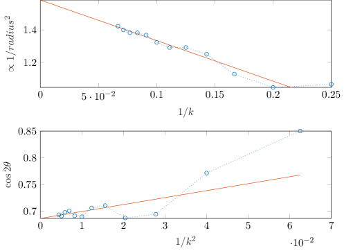
Figure 2: Mercer & Roberts (1990) [Appendix] plot for the series in heterogeneity $a$ of the coefficient of $U_{1}$ in a high-order extension of eq. 3.4b for $U_{1t}$. The extrapolated intercepts to $1/k=0$ predict the location of convergence limiting singularities in the complex $a$-plane.

fig. 2 shows a Mercer–Roberts plot for the coefficient of $U_{1}$ in $U_{1t}$, the plot for the coefficient of $U_{0xx}$ in $U_{0t}$ is almost the same. A simpler Domb–Sykes plot suffices for the other series (Domb & Sykes 1957, Hunter 1987, e.g.). Such plots predict the radius of convergence limiting singularity in heterogeneity $a$ as $1.21\mathchar 8507\relax{}1.21\mathchar 8507\relax{}1.57$, respectively, due to singularities in the complex $a$-plane at respective angles $23^{\circ}\mathchar 8507\relax{}23^{\circ}\mathchar 8507\relax{}90^{\circ}$ to the real-$a$ axis. Remarkably, the predicted radius of convergence $1.21$ indicates that we may use the three-mode homogenisation model even up to the extreme contrast heterogeneity of $a\to 1$.

Practically, the radius of convergence indicates that via expansion to errors $\mathcal{O}\mathchoice{\big{(}a^{11}\big{)}}{\big{(}a^{11}\big{)}}{(a^{11})}{(a^{11})}$ one would compute coefficients to four decimal places over the range $|a|<1/2$. Further exploration indicates that the $[6,6]$ Pade approximations in $a$ appear to be similarly accurate over the range $|a|\leq 1$ .

3.2.2 Convergence in spatial wavenumber

Recall that traditional mathematical proofs of homogenisation require the scale separation limit that the length-scale ratio $\ell/L\to 0$. In practice, engineers and scientists presume that $\ell/L<0.1$ or $0.01$ is sufficient. For example, Somnic & Jo (2022) comments [p.4] “For a periodic network of lattices to be considered as material, the characteristic length of its cells needs to be at least one or two orders of magnitude below the medium?s overall length scale.” By exploring the modal evolution eq. 3.4 to high-order in spatial gradients $\partial_{x}$, albeit to low-order in heterogeneity $a$, we here quantify the range of valid scale ratios $\ell/L$.

Choosing errors $\mathcal{O}\mathchoice{\big{(}a^{4}\big{)}}{\big{(}a^{4}\big{)}}{(a^{4})}{(a^{4})}$, amazingly we find the evolution effectively truncates. The computer algebra derives the invariant manifold evolution to $\mathcal{O}\mathchoice{\big{(}\partial_{x}^{31},a^{4}\big{)}}{\big{(}\partial_{x}^{31},a^{4}\big{)}}{(\partial_{x}^{31},a^{4})}{(\partial_{x}^{31},a^{4})}$ in just a few seconds. After a spatial Fourier transform to wavenumber $k$, some Domb–Sykes plots in powers of wavenumber $k$ of the $a^{2},a^{3}$ terms then shows all are limited by simple pole singularities at wavenumber $k=\pm 3/2$ .

A first consequence is that these Domb–Sykes plots show that for small heterogeneity the tri-continuum modelling resolves all wavenumbers $|k|<3/2$; that is, all wavelengths bigger than $4\pi/3=2\ell/3$. That is, potentially the resolved macroscales are all wavelengths bigger than just $2/3$ of the microscale periodicity! However, a practical lower bound may be about twice this. Moreover, be aware that higher orders in heterogeneity $a$ appear to be more restrictive Roberts (2024).

A second consequence is that the tri-continuum, three-mode, homogenisation algebraically simplifies using the nonlocal operator ${\mathcal{D}}:=(1+4/9\,\partial_{x}^{2})^{-1}$. appendix A finds the following to arbitrarily high order in $\partial_{x}$:

$$U_{0t} =(1+\tfrac{1}{2}a^{2})U_{0xx}-\tfrac{1}{2}aU_{1x}-\tfrac{1}{2}aU_{2xx}-\tfrac{1}{72}a^{3}{\mathcal{D}}(15\partial_{x}+11\partial^{3}+3\partial_{x}^{5})U_{1}$$

$$\quad{}-\tfrac{1}{72}a^{3}{\mathcal{D}}(11\partial_{x}^{2}+5\partial_{x}^{4})U_{2}+\mathcal{O}\mathchoice{\big{(}a^{4}\big{)}}{\big{(}a^{4}\big{)}}{(a^{4})}{(a^{4})},$$ (3.5a)

$$U_{1t} =-U_{1}-2U_{2x}+aU_{0x}+U_{1xx}-\tfrac{1}{36}a^{2}{\mathcal{D}}(15+18\partial_{x}^{2}+5\partial_{x}^{4})U_{1}$$

$$\quad{}-\tfrac{1}{18}a^{2}{\mathcal{D}}(4\partial_{x}+4\partial_{x}^{3}+\partial_{x}^{5})U_{2}+\tfrac{1}{144}a^{3}{\mathcal{D}}(60\partial_{x}+56\partial_{x}^{3}+13\partial_{x}^{5})U_{0}$$

$$\quad{}+\mathcal{O}\mathchoice{\big{(}a^{4}\big{)}}{\big{(}a^{4}\big{)}}{(a^{4})}{(a^{4})},$$ (3.5b)

$$U_{2t} =-U_{2}+2U_{1x}-aU_{0xx}+U_{2xx}+\tfrac{1}{36}a^{2}{\mathcal{D}}(3+8\partial_{x}^{2}+3\partial_{x}^{4})U_{2}$$

$$\quad{}+\tfrac{1}{18}a^{2}{\mathcal{D}}(4\partial_{x}+4\partial_{x}^{3}+\partial_{x}^{5})U_{1}-\tfrac{1}{72}a^{3}{\mathcal{D}}(22\partial_{x}^{2}+12\partial_{x}^{4}+\partial_{x}^{6})U_{0}$$

$$\quad{}+\mathcal{O}\mathchoice{\big{(}a^{4}\big{)}}{\big{(}a^{4}\big{)}}{(a^{4})}{(a^{4})},$$ (3.5c)

Through the nonlocal $\mathcal{D}$, such an model is an example of a nonlocal homogenisation (e.g., Bažant & Jirásek 2002).

Effects of higher order than cubic in $a$ have yet to be explored in detail. However, plots like fig. 2 for terms $a^{4}$ in heterogeneity indicate convergence limiting singularities at wavenumber $k=\pm 1/2$. That is, although for small $a$ we can get the above ‘exact’ nonlocal model, at finite heterogeneity $a$ singularities limit the homogenisation to macroscales longer than twice the length $\ell$ of the microscale period, as also found by Roberts (2024) for one-mode homogenisation. Thus, more generally, the high-order homogenisation is valid for macroscale $L>2\ell$ , equivalently, it is valid for scale ratios $\ell/L<0.5$ (although a practical bound might be a half of this), which is significantly better than the “one or two orders of magnitude” usually assumed.

3.3 Homogenise heterogeneous nonlinearity

Homogenising nonlinear heterogeneous systems requires just a few straightforward modifications. section 5 establishes its theoretical support. Here consider constructing a one-mode homogenisation of the heterogeneous diffusion eq. 2.1 with the addition of nonlinear advection, namely

$$\mathchoice{\frac{\partial u}{\partial t}}{{\partial u}/{\partial t}}{{\partial u}/{\partial t}}{{\partial u}/{\partial t}}=\mathchoice{\frac{\partial}{\partial x}}{{\partial}/{\partial x}}{{\partial}/{\partial x}}{{\partial}/{\partial x}}\left\{\kappa(x)\mathchoice{\frac{\partial u}{\partial x}}{{\partial u}/{\partial x}}{{\partial u}/{\partial x}}{{\partial u}/{\partial x}}-\gamma\eta(x)u^{2}/2\right\},\quad 0<x<L\,.$$ (3.6)

This is a Burgers’ pde with nonlinearity strength parametrised by $\gamma$, and heterogeneous coefficient in both the diffusion and nonlinear advection term, $\kappa(x)$ and $\eta(x)$ respectively. Let’s non-dimensionalise on the microscale length $\ell$ so that the heterogeneities $\kappa(x)$ and $\eta(x)$ are $2\pi$-periodic: specifically

$$\kappa(\theta):=1/(1+a\cos\theta), \eta(\theta):=c_{1}\cos\theta+c_{2}\sin 2\theta\,.$$ (3.7)

The corresponding phase-shift embedding modifies pde eq. 2.4 to the nonlinear

$$\mathchoice{\frac{\partial{\mathfrak{u}}}{\partial t}}{{\partial{\mathfrak{u}}}/{\partial t}}{{\partial{\mathfrak{u}}}/{\partial t}}{{\partial{\mathfrak{u}}}/{\partial t}}=\left(\mathchoice{\frac{\partial}{\partial x}}{{\partial}/{\partial x}}{{\partial}/{\partial x}}{{\partial}/{\partial x}}+\mathchoice{\frac{\partial}{\partial\theta}}{{\partial}/{\partial\theta}}{{\partial}/{\partial\theta}}{{\partial}/{\partial\theta}}\right)\left\{\kappa(\theta)\left(\mathchoice{\frac{\partial{\mathfrak{u}}}{\partial x}}{{\partial{\mathfrak{u}}}/{\partial x}}{{\partial{\mathfrak{u}}}/{\partial x}}{{\partial{\mathfrak{u}}}/{\partial x}}+\mathchoice{\frac{\partial{\mathfrak{u}}}{\partial\theta}}{{\partial{\mathfrak{u}}}/{\partial\theta}}{{\partial{\mathfrak{u}}}/{\partial\theta}}{{\partial{\mathfrak{u}}}/{\partial\theta}}\right)-\gamma\eta(\theta){\mathfrak{u}}^{2}/2\right\},$$ (3.8)

for fields ${\mathfrak{u}}$ being $2\pi$-periodic in $\theta$. As an example, we construct the one-mode invariant manifold homogenisation ($M=1$) of this embedding pde. The accessible class of manifolds is to construct homogenisations as a regular perturbation in nonlinearity parameter $\gamma$. There are just three necessary changes in the computer algebra of appendix A: firstly, truncating to some specified order of error in $\gamma$, here choose errors $\mathcal{O}\mathchoice{\big{(}\gamma^{2}\big{)}}{\big{(}\gamma^{2}\big{)}}{(\gamma^{2})}{(\gamma^{2})}$; secondly, specifying the extra heterogeneity $\eta(\theta)$; and thirdly, modifying the computation of the residual by including the additional term $-\gamma\eta(\theta){\mathfrak{u}}^{2}/2$ in the flux.

Executing the code of appendix A constructs the one-mode homogenisation and finds that the invariant manifold ensemble field (to low-order)

$${\mathfrak{u}} =U_{0}+a\sin\theta\,U_{0x}+\gamma c_{1}(\tfrac{1}{2}\sin\theta+\tfrac{1}{8}a\sin 2\theta)U_{0}^{2}$$

$$\quad{}-\gamma c_{2}(\tfrac{1}{4}a\cos\theta+\tfrac{1}{4}\cos 2\theta+\tfrac{1}{12}a\cos 3\theta)U_{0}^{2}+\mathcal{O}\mathchoice{\big{(}\gamma^{2}+\partial_{x}^{2},a^{2}\big{)}}{\big{(}\gamma^{2}+\partial_{x}^{2},a^{2}\big{)}}{(\gamma^{2}+\partial_{x}^{2},a^{2})}{(\gamma^{2}+\partial_{x}^{2},a^{2})}.$$ (3.9a)

Simultaneously the code constructs that the evolution on the invariant manifold obeys the homogenised pde

$$U_{0t}=U_{0xx}-\tfrac{1}{4}\gamma\partial_{x}\big{(}c_{1}aU_{0}^{2}+c_{2}a^{2}U_{0}U_{0x}\big{)}+\mathcal{O}\mathchoice{\big{(}\gamma^{2},\partial_{x}^{3},a^{3}\big{)}}{\big{(}\gamma^{2},\partial_{x}^{3},a^{3}\big{)}}{(\gamma^{2},\partial_{x}^{3},a^{3})}{(\gamma^{2},\partial_{x}^{3},a^{3})}.$$ (3.9b)

Although the microscale nonlinear advection coefficient has coefficient with zero-mean, $\overline{\eta(\theta)}=0$, nonetheless the interaction of the two heterogeneities (3.7) generates a non-zero effective nonlinear advection${}\approx-\frac{1}{2}\gamma c_{1}aU_{0}U_{0x}$.

4 An example of high-contrast multi-continuum homogenisation

The modelling of materials with so-called high contrast is of interest (e.g., Leung 2024, Efendiev & Leung 2023, Chen et al. 2023). This section considers the specific example of the multiscale embedding pde eq. 2.1 with a high-contrast, $\ell$-periodic, heterogeneous coefficient $\kappa(x)$. Specifically, in each microscale period, the coefficient $\kappa(x)=\kappa_{1}$ constant for most $x$, except in a thin near-insulating layer of width $\eta\ll\ell$ where the coefficient $\kappa(x)=\kappa_{0}\ll\kappa_{1}$. We focus on modelling interesting dynamics in the interior $\mathbb{X}$ of the relatively large 1-D spatial domain $[0,L]$.

This section shows how the novel and powerful invariant manifold framework of section 2 establishes rigorous multi-mode multi-continuum homogenisations of the high-contrast material. For example, section 4.3 addresses the bi-continuum case and derives the homogenised model in terms of two physics-informed macroscale quantities $U_{0},U_{1}$ that evolve according to two coupled macroscale pdes of the form, non-dimensionalised,

$$\partial_{t}^{\alpha}U_{0}=0.81U_{0xx}+0.36U_{1x}+\cdots,\quad\partial_{t}^{\alpha}U_{1}=-0.46U_{1}-0.36U_{0x}+\cdots,\quad$$ (4.1)

where here the numerical coefficients are for a specific high-contrast case in the class defined above, and for both $\alpha=1,2$ .

Because our sound modelling is transitive, the corresponding classic homogenised one-mode macroscale pde eq. 2.2 may be recovered by the adiabatic quasi-equilibrium approximation of the second mode in eq. 4.1 that gives $U_{1}\approx-0.77U_{0x}$ . Thence the first pde of eq. 4.1 reduces quantitatively to the usual homogenised macroscale pde $\partial_{t}^{\alpha}U_{0}\approx 0.54U_{0xx}$ .

Extensions to more than two modes are straightforward: for example, section 4.4 derives a tri-continuum model. Indeed the number $M$ of modes is coded as a parameter in the computer algebra code of appendix B.

As introduced in section 2, and detailed in section 5.2, the theoretical support for such homogenisation depends upon the time operator $\partial_{t}^{\alpha}$. For the diffusive case, $\alpha=1$, the homogenised models are known to generally be exponentially quickly emergent. For the wave case, $\alpha=2$, the homogenised models are best viewed as a guiding centre for the dynamics. In all cases, backwards theory (adapted from Roberts 2022, Hochs & Roberts 2019) would assert that there is a system close to the specified pde eq. 2.1 that has the precise constructed invariant manifold and associated homogenisation, such as eq. 4.1.

Recall that the approach here makes rigorous progress through considering the ensemble of all phase-shifts by solving the pde eq. 2.4 in the ‘cylindrical’ domain ${\mathbb{D}}:=\{({{\cal\mathchoice{\scriptstyle X}{\scriptstyle X}{\scriptscriptstyle X}{\scriptscriptstyle X}}},\theta):{{\cal\mathchoice{\scriptstyle X}{\scriptstyle X}{\scriptscriptstyle X}{\scriptscriptstyle X}}}\in{\mathbb{X}}\mathchar 8507\relax{}\theta\in[-\ell/2,\ell/2]\}$, and with $\ell$-periodic boundary conditions in $\theta$. section 2.1 established that solutions of eq. 2.4 provide us with solutions to the heterogeneous pde eq. 2.1.

To establish the basis of an invariant manifold homogenisation, recall that we consider the embedding pde (2.4) with $\mathchoice{\frac{\partial}{\partial{{\cal\mathchoice{\scriptstyle X}{\scriptstyle X}{\scriptscriptstyle X}{\scriptscriptstyle X}}}}}{{\partial}/{\partial{{\cal\mathchoice{\scriptstyle X}{\scriptstyle X}{\scriptscriptstyle X}{\scriptscriptstyle X}}}}}{{\partial}/{\partial{{\cal\mathchoice{\scriptstyle X}{\scriptstyle X}{\scriptscriptstyle X}{\scriptscriptstyle X}}}}}{{\partial}/{\partial{{\cal\mathchoice{\scriptstyle X}{\scriptstyle X}{\scriptscriptstyle X}{\scriptscriptstyle X}}}}}$ neglected, and solved with $\ell$-periodic boundary conditions. This describes the basic physical sub-cell dynamics. Because the pde is linear, it is sufficient to consider the dynamics about the zero equilibrium, which we do henceforth.

4.1 Spectrum at each equilibrium

The approach is to choose invariant manifold models (Roberts 2015a) based upon the sub-cell physics encoded in the spectrum of the cell problem eq. 2.6, and to choose depending upon required macroscale aspects.

The spectrum of the cell problem is in turn determined from the eigenvalues of the operator on the right-hand side of the cell-problem eq. 2.6 with its $\ell$-periodic boundary conditions. Say the eigenvalues are $\lambda_{0}=0\geq\lambda_{1}\geq\lambda_{2}\geq\cdots$ with corresponding eigenfunctions $v_{0}(\theta)\mathchar 8507\relax{}v_{1}(\theta)\mathchar 8507\relax{}v_{2}(\theta)\mathchar 8507\relax{}\ldots$ , such as the example eigenfunctions drawn in fig. 3.

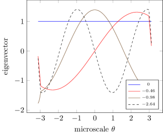
Figure 3: an example of the leading four eigenfunctions of the cell-problem eq. 2.6, and corresponding eigenvalues, for a high-contrast heterogeneity. For the non-dimensional case of $\ell=2\pi$, $\kappa_{1}=1$, and a thin insulating layer $\eta/\ell=0.06$ located at $\theta=\pm\pi$ of insulation, $\kappa_{0}=0.06$ ($\chi=1$).

Consequently, the two common cases of the cell problem are the following two:

• for diffusion, $\alpha=1$, the modal solutions of the cell problem eq. 2.6 are that ${\mathfrak{u}}\propto\operatorname{e}^{\lambda_{m}t}$ for eigenvalues $0\mathchar 8507\relax{}\lambda_{1}\mathchar 8507\relax{}\lambda_{2}\mathchar 8507\relax{}\ldots$;

• whereas for waves, $\alpha=2$, the modal solutions of the cell problem eq. 2.6 are that ${\mathfrak{u}}\propto\operatorname{e}^{\pm\operatorname{i}\omega_{m}t}$ for frequencies $\omega_{m}:=\sqrt{-\lambda_{m}}$;

• and the modal solutions are otherwise for other time evolution operators $\partial_{t}^{\alpha}$ (e.g., section 5.2.4).

Generally we choose to focus on, that is model, the sub-cell modes associated with the small magnitude eigenvalues because these are either the emergent sub-cell modes, $\alpha=1$, or the guiding centre sub-cell modes, $\alpha=2$ (e.g., van Kampen 1985), respectively.

For the specific example leading to the model eq. 4.1, the non-dimensional spectrum for diffusion is $\lambda_{m}\kappa_{1}4\pi^{2}/\ell^{2}\in\{0\mathchar 8507\relax{}{-0.46}\mathchar 8507\relax{}{-0.98}\mathchar 8507\relax{}\ldots\}$, whereas the non-dimensional frequencies for waves are $\sqrt{\lambda_{m}\kappa_{1}}2\pi/\ell\in\{0\mathchar 8507\relax{}{\pm\operatorname{i}0.68}\mathchar 8507\relax{}{\pm\operatorname{i}0.99}\mathchar 8507\relax{}\ldots\}$ (the zero frequency has multiplicity two). The model pde eq. 4.1 is constructed by forming the approximate invariant manifold based upon the two/four slowest modes (blue and red eigenfunctions in the example of fig. 3) corresponding to non-dimensional cell-problem eq. 2.7 diffusive eigenvalues $\{0\mathchar 8507\relax{}{-0.46}\}$ or wave frequencies $\{0\mathchar 8507\relax{}{\pm\operatorname{i}0.68}\}$, respectively.

Recall from section 2.2.1 that a rational approach to forming multi-continuum models is then to decide what time-scales you need to resolve in the problem at hand, and then chose the number of leading modes whose eigenvalues/frequencies match or are slower than that of the needed time-scale. These leading modes then form the multi-continuum, or micromorphic, model.

For these spatio-temporal systems there is additionally the issue of spatial resolution. High-order approximations can indicate a quantitative limit to the spatial resolution as in section 3.2.2 (e.g., Mercer & Roberts 1994, Watt & Roberts 1995). A guiding ‘rule-with-exceptions’ is that the more the number of modes forming the invariant manifold then the shorter the resolved length scales of the multi-mode model. This issue was extensively discussed for shear dispersion by Watt & Roberts (1995) [§§2.1, 2.3, 3.4, 4.1]. Nonetheless, such high-order evidence is only a guide: since we mostly use low-order models, the practical issue is primarily whether a chosen low-order has adequate spatial resolution for the purposes at hand. The quantitative error estimate by equation (23) of Roberts (2015a) is potentially more useful for such low-order modelling.

4.1.1 High-contrast thin layer

To homogenise the high contrast problem we need to determine the spectrum of the eigen-problem eq. 2.7. We first analytically approximate the eigenvalue spectrum in cases when a layer of near ‘insulator’ is so thin that we can replace it by a ‘jump’ condition (as suggested by the example eigenfunctions of fig. 3). These analytic approximations guide subsequent numerical-algebraic construction and interpretation. We deduces that eigenvalues are $\lambda_{m}\approx-m^{2}\kappa_{1}\pi^{2}/\ell^{2}$ corresponding to eigenfunctions, over the cell $\theta\in(-\ell/2,+\ell/2)$, of $v_{m}\approx\cos(m\pi\theta/\ell)$ for even $m=0,2,4,\ldots$ , and, with a ‘jump’ across the layer at $\theta=\pm\ell/2$, of $v_{m}\approx\sin(m\pi\theta/\ell)$ for odd $m=1,3,5,\ldots$ .

We seek solutions to the eigen-problem eq. 2.7 for the right-hand side operator. That is, we find $\ell$-periodic solutions to

$$\kappa_{1}v_{\theta\theta}=\lambda v\text{ on }(-\ell/2,\ell/2),\quad\text{except in a layer where }\kappa_{0}v_{\theta\theta}=\lambda v\,,$$

for an ‘insulating’ layer of small thickness $\eta$ and where $\kappa_{0}=\mathcal{O}\mathchoice{\big{(}\eta\big{)}}{\big{(}\eta\big{)}}{(\eta)}{(\eta)}$. We know all eigenvalues $\lambda\leq 0$.

Thin insulating layer

Here derive jump conditions across the thin layer. For algebraic simplicity, temporarily set the origin of $\theta$ at the centre of the thin layer so the layer is the interval $(-\eta/2,+\eta/2)$.

Within the thin layer an eigenfunction is of the form $v=C\cos\big{(}\sqrt{-\lambda/\kappa_{0}}\theta\big{)}+D\sin\big{(}\sqrt{-\lambda/\kappa_{0}}\theta\big{)}$. Define

$$[v]:=v_{\eta/2}-v_{-\eta/2}=2D\sin\big{(}\sqrt{-\lambda/\kappa_{0}}\eta/2\big{)}=D\sqrt{-\lambda/\kappa_{0}}\eta+\mathcal{O}\mathchoice{\big{(}\eta^{3/2}\big{)}}{\big{(}\eta^{3/2}\big{)}}{(\eta^{3/2})}{(\eta^{3/2})};$$

$$\overline{v}:=\tfrac{1}{2}(v_{\eta/2}+v_{-\eta/2})=C\cos\big{(}\sqrt{-\lambda/\kappa_{0}}\eta/2\big{)}=C+\mathcal{O}\mathchoice{\big{(}\eta\big{)}}{\big{(}\eta\big{)}}{(\eta)}{(\eta)}.$$

Hence $C\approx\overline{v}=\mathcal{O}\mathchoice{\big{(}1\big{)}}{\big{(}1\big{)}}{(1)}{(1)}$ and $D\approx[v]/\big{(}\sqrt{-\lambda/\kappa_{0}}\eta\big{)}=\mathcal{O}\mathchoice{\big{(}\eta^{-1/2}\big{)}}{\big{(}\eta^{-1/2}\big{)}}{(\eta^{-1/2})}{(\eta^{-1/2})}$. Then within the layer the derivative

$$v_{\theta} =-\sqrt{-\lambda/\kappa_{0}}C\sin\big{(}\sqrt{-\lambda/\kappa_{0}}\theta\big{)}+\sqrt{-\lambda/\kappa_{0}}D\cos\big{(}\sqrt{-\lambda/\kappa_{0}}\theta\big{)}$$

$$\approx-\sqrt{-\lambda/\kappa_{0}}\overline{v}\sin\big{(}\sqrt{-\lambda/\kappa_{0}}\theta\big{)}+([v]/\eta)\cos\big{(}\sqrt{-\lambda/\kappa_{0}}\theta\big{)}.$$

So the jump and the mean of the derivative are

$$[v_{\theta}]\approx-2\sqrt{-\lambda/\kappa_{0}}\overline{v}\sin\big{(}\sqrt{-\lambda/\kappa_{0}}\eta/2\big{)}\approx(\lambda\eta/\kappa_{0})\overline{v}\,,$$

$$\overline{v_{\theta}}\approx([v]/\eta)\cos\big{(}\sqrt{-\lambda/\kappa_{0}}\eta/2\big{)}\approx[v]/\eta\,.$$

Outside the layer

The eigenfunctions $v(\theta)$ are to be continuous so the jump $[v]$ and mean $\overline{v}$ are the same inside and outside the layer. And the flux has to be continuous across the layer boundary, that is $\kappa_{1}v_{\theta}^{\text{outside}}=\kappa_{0}v_{\theta}^{\text{inside}}$. Hence outside the layer we have the conditions

$$[v_{\theta}]=\big{[}(\kappa_{0}/\kappa_{1})v_{\theta}^{\text{inside}}\big{]}\approx(\lambda\eta/\kappa_{1})\overline{v}\,,$$ (4.2a)

$$\overline{v_{\theta}}=\overline{(\kappa_{0}/\kappa_{1})v_{\theta}^{\text{inside}}}\approx\kappa_{0}/(\kappa_{1}\eta)[v]=1/(\chi\ell)[v]$$ (4.2b)

as we choose to scale $\kappa_{0}$ so that $\kappa_{0}/\kappa_{1}=\eta/(\chi\ell)$ for some insulating parameter $\chi$. That is, the layer diffusivity/elasticity $\kappa_{0}\propto\eta\kappa_{1}$ decreases with the relative layer thickness $\eta/\ell$. Thus small $\eta$ characterises a high-contrast material. Parameter $\chi$ characterises the strength of the ‘insulation’ in the thin layer: larger is more insulating, whereas smaller is less so.

For algebraic simplicity we now reset the origin of $\theta$ so that the thin layer is at $\theta=\pm\ell/2$, and hence a jump across the thin layer is hereafter $[v]=v_{-\ell/2}-v_{+\ell/2}$.

There are two families of eigenfunctions and eigenvalues.

• The symmetric family is eigenfunctions $v=\cos k\theta$ for eigenvalue $\lambda=-\kappa_{1}k^{2}$ for some wavenumbers $k$ to be determined. For this eigenfunction

  $$\overline{v}=\cos(k\ell/2), [v]=0, \overline{v_{\theta}}=0, [v_{\theta}]=2k\sin(k\ell/2).\lambda$$

  Hence eq. 4.2b is satisfied, whereas eq. 4.2a requires that $2k\sin(k\ell/2)=-k^{2}\eta\cos(k\ell/2)$, that is, $2k\tan(k\ell/2)=-k^{2}\eta\to 0$ as $\eta\to 0$ . Hence these eigenfunctions occur for wavenumber $k=m\pi/\ell$ for even integer $m$. That is, $v_{m}=\cos(m\pi\theta/\ell)$ and corresponding eigenvalues $\lambda_{m}=-\kappa_{1}\pi^{2}m^{2}/\ell^{2}$ for $m=0,2,4,\ldots$. table 1 list the first two of these eigenvalues, $\lambda_{0},\lambda_{2}$, for four selected parameters $\chi$ of thin insulation layer width $\eta$.

  Table 1: first two ${\mathfrak{K}}$-values that solve $\tan{\mathfrak{K}}=-\chi{\mathfrak{K}}$ for four values of insulation strength $\chi$. Below are the leading four eigenvalues for the non-dimensional case of $\kappa_{1}=1$ and $\ell=2\pi$ : these approximate the eigenvalues for small insulation layer width $\eta$.

  $\begin{array}[]{l|llll}\chi&1/3&1&3&9\\ \hline\cr{\mathfrak{K}}_{1}&2.46&2.03&1.74&1.63\\ {\mathfrak{K}}_{3}&5.23&4.91&4.78&4.74\\ \hline\cr\lambda_{0}&0&0&0&0\\ \lambda_{1}&-0.61&-0.42&-0.31&-0.27\\ \lambda_{2}&-1&-1&-1&-1\\ \lambda_{3}&-2.77&-2.45&-2.32&-2.27\\ \hline\cr\end{array}$

• The asymmetric family is eigenfunctions of the form $v=\sin k\theta$ for eigenvalue $\lambda=-\kappa_{1}k^{2}$ for some wavenumbers $k$ to be determined. For this eigenfunction

  $$\overline{v}=0, [v]=-2\sin(k\ell/2), \overline{v_{\theta}}=k\cos(k\ell/2), [v_{\theta}]=0.$$

  Hence eq. 4.2a is satisfied, whereas eq. 4.2b requires that $k\cos(k\ell/2)=-2/(\chi\ell)\sin(k\ell/2)$,

  $$\text{that is, }\tan(k\ell/2)=-\chi(k\ell/2).$$ (4.3)

  For odd integer $m$, let ${\mathfrak{K}}_{m}$ be the solutions of $\tan{\mathfrak{K}}=-\chi{\mathfrak{K}}$ in sequence so that $m\pi/2<{\mathfrak{K}}_{m}\leq(m+1)\pi/2$. Then wavenumber $k=2{\mathfrak{K}}_{m}/\ell$ satisfies eq. 4.3 and so asymmetric eigenfunctions are $v_{m}=\sin(2{\mathfrak{K}}_{m}\theta/\ell)$ corresponding to eigenvalues $\lambda_{m}=-\kappa_{1}4{\mathfrak{K}}_{m}^{2}/\ell^{2}$ for $m=1,3,\ldots$ . table 1 list the first two of these eigenvalues, $\lambda_{1},\lambda_{3}$, for four selected parameters $\chi$ of thin insulation layer width $\eta$.

4.2 One-mode slow manifold model

One may construct a slow manifold model based upon the eigenvalue zero, here corresponding to the one sub-cell mode $v_{0}=\cos 0\theta=1$. Since $v_{0}$ is constant, such slow invariant manifold modelling gives the classic homogenised pde eq. 2.2, but generalised to higher-order derivatives at finite scale separation (Roberts 2024). In the diffusion case, $\alpha=1$, the argument for its emergence as a valid model is that all other sub-cell modes decay exponentially quickly in time, the slowest of which is $\exp({-\kappa_{1}4{\mathfrak{K}}_{1}^{2}t/\ell^{2}})$.

Let’s explore the non-dimensional case of $\kappa_{1}=1$ and $\ell=2\pi$ (table 1) with the specific insulating thin layer $\eta/\ell=\kappa_{0}=0.06$ (i.e., $\chi=1$). All the cell-problems are solved numerical on a sub-cell grid with 128 points per cell. The numerically obtained leading non-zero eigenvalue is $\lambda_{1}=-0.4597$, so in the diffusion case the decay to the slow manifold homogenisation is roughly like $\operatorname{e}^{-0.46\,t}$, from any given initial condition. The computer algebra of appendix B, with modes $M=1$, then seeks a slow manifold that satisfies the embedding pde eq. 2.4 (discretised in $\theta$) to any specified order in $\partial_{x}$. The result is that the detailed slow manifold field is

$${\mathfrak{u}}(t,x,\theta)=U_{0}+u_{1}(\theta)U_{0x}+u_{2}(\theta)U_{0xx}+\mathcal{O}\mathchoice{\big{(}\partial_{x}^{3}\big{)}}{\big{(}\partial_{x}^{3}\big{)}}{(\partial_{x}^{3})}{(\partial_{x}^{3})},$$ (4.4a)

in terms of the coefficient functions plotted in fig. 4.

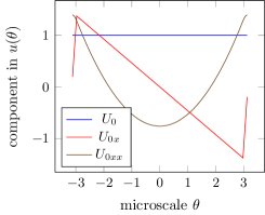
Figure 4: the sub-cell structure of the one-mode slow manifold field eq. 4.4a in the high-contrast thin-layer problem. Specifically, this is the non-dimensional case of $\ell=2\pi$, $\kappa_{1}=1$, and a thin insulating layer $\eta/\ell=0.06$ located at $\theta=\pm\pi$ of insulation parameter $\chi=1$ so $\kappa_{0}=0.06$.

For this high-contrast thin layer, the $U_{0x}$-component of fig. 4 shows that $x$-gradients of the field lead to a sub-cell field where rapid spatial variation takes place in the thin insulating layer, as expected physically. The corresponding, but higher-order, homogenised evolution is determined to be

$$\mathchoice{\frac{\partial^{\alpha}U_{0}}{\partial t^{\alpha}}}{{\partial^{\alpha}U_{0}}/{\partial t^{\alpha}}}{{\partial^{\alpha}U_{0}}/{\partial t^{\alpha}}}{{\partial^{\alpha}U_{0}}/{\partial t^{\alpha}}}=0.5386\,U_{0xx}+0.3379\,U_{0xxxx}-0.9019\,U_{0xxxxxx}+\mathcal{O}\mathchoice{\big{(}\partial_{x}^{7}\big{)}}{\big{(}\partial_{x}^{7}\big{)}}{(\partial_{x}^{7})}{(\partial_{x}^{7})},$$ (4.4b)

that is, $K=0.5386$ in the leading-order homogenised pde eq. 2.2. Higher-order models such as eq. 4.4b often need regularisation: for example, upon neglecting the sixth-order derivative, the model eq. 4.4b may be regularised to $(1-0.63\partial_{x}^{2})\partial_{t}^{\alpha}U_{0}\approx 0.54\,U_{0xx}$ (to two decimal places). An alternative form of this regularised pde is the nonlocal homogenisation $\partial_{t}^{\alpha}U_{0}\approx 0.54\,{\mathcal{A}}\star U_{0xx}$ in terms of the convolution kernel ${\mathcal{A}}(x)\propto\exp(-0.79\,|x|)$, a kernel which decays to zero on the heterogeneity length $\ell$, here $2\pi$. Bažant & Jirásek (2002) discussed how such nonlocal models may desirably capture small-scale effects, produce convergent numerical solutions, achieve regularisation, and capture size effects seen in experiments.

4.3 Two-mode, bi-continuum, homogenisations exist and emerge

A two-mode, invariant manifold, homogenisation may be constructed based upon the leading two eigenvalues. For definiteness we non-dimensionalise space-time so that cell-length $\ell=2\pi$ and the coefficient $\kappa_{1}=1$, and also focus on the case of thin layer parameter $\chi=1$, the second column of table 1.

In this case the leading two eigenvalues are $\lambda_{0}=0$ and $\lambda_{1}\approx-0.42$ corresponding to the two sub-cell modes $v_{0}=1$ and $v_{1}\approx\sin(2.03\,\theta/\pi)$ (the two blue curves in the two panels of fig. 5 are more precise). In the diffusion case, $\alpha=1$, and since the next eigenvalue $\lambda_{2}=-1$, such a two-mode model is emergent with the slowest transient decaying roughly like $\operatorname{e}^{-t}$. The eigenvalue gap of $(-0.42,-1)$ caters for perturbing macroscale $x$-gradients.

To construct the invariant manifold homogenisation corresponding to these two modes we employ the algorithm summarised in section 2.2.3, and starting from the initial approximation that ${\mathfrak{u}}\approx U_{0}+U_{1}v_{1}(\theta)$ such that $\partial_{t}^{\alpha}U_{0}\approx 0$ and $\partial_{t}^{\alpha}U_{1}\approx-0.42\,U_{1}$ . The computer algebra of appendix B then iteratively corrects its approximations until the governing embedding pde eq. 2.4 has residual smaller than a specified order of error.

Here we modify in two ways the procedure that is introduced in section 2.2.3 and as implemented in the example of section 3.1. Firstly, previously we had introduced and implemented the procedure as if we could do all steps exactly in algebra. But for this high-contrast media we do not have exact algebraic expressions for the eigenfunctions (section 4.1.1). Consequently, we adopt a simple sub-cell $\theta$-space discretisation of the cell eigen-problem eq. 2.7 and the corresponding homological equation eq. 2.9. The computer algebra sets $n=128$ points per period of sub-cell variable $\theta$, and uses centred differences in $\theta$, which should be fine enough to be faithful to the microscale differentials to about four significant digits. The macroscale variations in $x,{\text{\boldmath$\cal\mathchoice{\scriptstyle X}{\scriptstyle X}{\scriptscriptstyle X}{\scriptscriptstyle X}$}}$ are still represented explicitly in algebra—there is no numerical approximation on the macroscale. MacKenzie (2005) first discussed such fine-grid numerics for constructing invariant manifolds of the macroscale dynamics of the 1-D and 2-D Kuramoto–Sivashinky pde and the need for numerics in 2-D (see also Roberts et al. 2014). section 6 also uses such mixed numerics-algebra for multi-continuum homogenisation of 2-D elasticity.

The second modification is that for generalised multi-continua homogenisation it is awkward to code solutions to the homological equation eq. 2.9 when it involves modes with non-zero eigenvalue/frequency. Instead we more quickly code simpler updates which just take more computer iterations to be accurate. The simplification is to omit the tricky terms $\sum_{m=0}^{M-1}\lambda_{m}\mathchoice{\frac{\partial v^{\prime}}{\partial U_{m}}}{{\partial v^{\prime}}/{\partial U_{m}}}{{\partial v^{\prime}}/{\partial U_{m}}}{{\partial v^{\prime}}/{\partial U_{m}}}U_{m}$ on the left-hand side of eq. 2.9. Then the left-hand side operator is a straightforward constant matrix which is efficiently inverted or LU-factored just once (section B.3) and used repeatedly. The updates $v^{\prime}$ and $G^{\prime}$ are then not exactly correct, but they are good enough to make progress. The error in the coefficients of $v$ and $G$ decrease each iteration by the ratio of the largest magnitude eigenvalue in the model to the smallest magnitude eigenvalue neglected by the model, here the ratio $|\lambda_{M-1}|/|\lambda_{M}|$. We simply let the computer do more iterations until the numerical error is small enough: appendix B sets a maximum relative error of $10^{-8}$. The numerical convergence is quicker for a larger spectral gap between $\lambda_{M-1}$ and $\lambda_{M}$.

We now explore the two-mode bi-continuum homogenisation to second order in macroscale gradients. Upon executing the code of appendix B, 25 iterations are sufficient to give the following detailed physics-informed sub-cell field to excellent numerical accuracy:

$${\mathfrak{u}}(t,x,\theta) =\phantom{v_{1}(\theta)}U_{0}+u_{01}(\theta)U_{0x}+u_{02}(\theta)U_{0xx}$$

$${}+v_{1}(\theta)U_{1}+u_{11}(\theta)U_{1x}+u_{12}(\theta)U_{1xx}+\mathcal{O}\mathchoice{\big{(}\partial_{x}^{3}\big{)}}{\big{(}\partial_{x}^{3}\big{)}}{(\partial_{x}^{3})}{(\partial_{x}^{3})},$$ (4.5a)

in terms of five coefficient functions plotted in fig. 5.

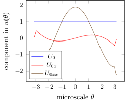
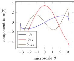
Figure 5: the sub-cell structure of the two-mode, bi-continuum, invariant manifold field eq. 4.5a in the high-contrast thin-layer problem. Specifically, the non-dimensional case of $\ell=2\pi$, $\kappa_{1}=1$, and a thin insulating layer $\eta/\ell=0.06$ located at $\theta=\pm\pi$ of insulation parameter $\chi=1$ so $\kappa_{0}=0.06$.

The corresponding, but to higher-order, homogenised model for the macroscale variables $U_{0},U_{1}$ is determined to be, for both $\alpha=1,2$,

$$\partial_{t}^{\alpha}{U_{0}} =\phantom{-0.4597\,U_{1}}+0.3552\,U_{1x}+0.8130\,U_{0xx}$$

$$\qquad{}+1.063\,U_{1xxx}+0.6146\,U_{0xxxx}+\mathcal{O}\mathchoice{\big{(}\partial_{x}^{5}\big{)}}{\big{(}\partial_{x}^{5}\big{)}}{(\partial_{x}^{5})}{(\partial_{x}^{5})},$$ (4.5b)

$$\partial_{t}^{\alpha}{U_{1}} =-0.4597\,U_{1}-0.3552\,U_{0x}-2.620\,U_{1xx}$$

$$\qquad{}-1.736\,U_{0xxx}-17.11\,U_{1xxxx}+\mathcal{O}\mathchoice{\big{(}\partial_{x}^{5}\big{)}}{\big{(}\partial_{x}^{5}\big{)}}{(\partial_{x}^{5})}{(\partial_{x}^{5})},$$ (4.5c)

These pdes form the two-mode, bi-continuum, homogenisation for this high-contrast material. As discussed in sections 2 and 5 this homogenisation is supported by extant rigorous theory. In application, one truncates the pdes eq. 4.5 to an order of error suitable for the purposes at hand (and possibly with some suitable regularisation). In solutions obtained using a truncated eq. 4.5, one could quantitatively estimate the modelling error via the remainder expression (23) of Roberts (2015a).

Sound modelling is transitive

The two-mode bi-continuum homogenisation eq. 4.5 itself has a slow manifold. For example, a low-order adiabatic approximation of eq. 4.5c gives $0\approx-0.4597\,U_{1}-0.3552\,U_{0x}$ , which leads to $U_{1}\approx-0.7727\,U_{0x}$ . Substituting this adiabatic approximation into eq. 4.5b gives $\mathchoice{\frac{\partial^{\alpha}U_{0}}{\partial t^{\alpha}}}{{\partial^{\alpha}U_{0}}/{\partial t^{\alpha}}}{{\partial^{\alpha}U_{0}}/{\partial t^{\alpha}}}{{\partial^{\alpha}U_{0}}/{\partial t^{\alpha}}}\approx(-0.3552\times 0.7727+0.8130)U_{0xx}=0.5385\,U_{0xx}$ . This adiabatic slow manifold pde model in just $U_{0}$ reproduces the leading order term of the slow manifold homogenisation constructed by the iteration of appendix B with one-mode ($M=1$), see the linear term in eq. 4.9a, and thus verifies the transitivity of our sound approach to homogenisation.

4.4 Three-mode, tri-continuum, homogenisation exist and emerge

A three-mode, tri-continuum, invariant manifold, homogenisation may be constructed based upon the leading three eigenvalues: for example, $\lambda=0,-0.42,-1$ in the nondimensional case $\chi=1$, $\ell=2\pi$, and $\kappa_{1}=1$ (table 1). The three corresponding sub-cell modes are $v_{0}=1$, $v_{1}\approx\sin 2\theta/\pi$ , and $v_{2}\approx\cos\theta$ (more precisely, the blue curves in the three panels of fig. 6). In the diffusive case, $\alpha=1$, such a three-mode homogenisation emerges with the slowest transient decaying roughly like $\operatorname{e}^{-2.5\,t}$ (table 1). That is, this three-mode homogenisation is valid over shorter times than the two-mode, bi-continuum, homogenisation eq. 4.5. The eigenvalue gap $(-1,-2.5)$ caters for the perturbing macroscale $x$-gradients.

The computer algebra of appendix B constructs the corresponding three-mode invariant manifold homogenisation by setting the parameter $M=3$ . The algorithm requires 19 iterations to find the detailed three-mode, tri-continuum, invariant manifold field is, to low-order,

$${\mathfrak{u}}(t,x,\theta) =\phantom{v_{1}(\theta)}U_{0}+u_{01}(\theta)U_{0x}+u_{02}(\theta)U_{0xx}$$

$${}+v_{1}(\theta)U_{1}+u_{11}(\theta)U_{1x}+u_{12}(\theta)U_{1xx}$$

$${}+v_{2}(\theta)U_{2}+u_{21}(\theta)U_{2x}+u_{22}(\theta)U_{2xx}+\mathcal{O}\mathchoice{\big{(}\partial_{x}^{3}\big{)}}{\big{(}\partial_{x}^{3}\big{)}}{(\partial_{x}^{3})}{(\partial_{x}^{3})},$$ (4.6a)

in terms of eight coefficient functions plotted in fig. 6.

Figure 6: the sub-cell structure of the three-mode, tri-continuum, invariant manifold field (section 4.4) in the high-contrast thin-layer problem. Specifically, the non-dimensional case of $\ell=2\pi$, $\kappa_{1}=1$, and a thin insulating layer $\eta/\ell=0.06$ located at $\theta=\pm\pi$ of insulation parameter $\chi=1$ so $\kappa_{0}=0.06$.

To higher-order, the corresponding evolution the of macroscale variables $U_{0},U_{1},U_{2}$ is determined to be, for both $\alpha=1,2$,

$$\partial_{t}^{\alpha}{U_{0}} =\phantom{-0.4597\,U_{1}}+0.3552\,U_{1x}+0.8130\,U_{0xx}+0.5191\,U_{2xx}$$

$$\quad{}-0.2714\,U_{1xxx}-0.07643\,U_{0xxxx}-0.3184\,U_{2xxxx}+\mathcal{O}\mathchoice{\big{(}\partial_{x}^{5}\big{)}}{\big{(}\partial_{x}^{5}\big{)}}{(\partial_{x}^{5})}{(\partial_{x}^{5})},$$ (4.6b)

$$\partial_{t}^{\alpha}{U_{1}} =-0.4597\,U_{1}-0.3552\,U_{0x}-1.339\,U_{2x}+0.8218\,U_{1xx}$$

$$\quad{}+0.04649\,U_{0xxx}-0.4531\,U_{2xxx}+0.5182\,U_{1xxxx}+\mathcal{O}\mathchoice{\big{(}\partial_{x}^{5}\big{)}}{\big{(}\partial_{x}^{5}\big{)}}{(\partial_{x}^{5})}{(\partial_{x}^{5})},$$ (4.6c)

$$\partial_{t}^{\alpha}{U_{2}} =-0.9804\,U_{2}+1.339\,U_{1x}+0.3918\,U_{0xx}-0.2717\,U_{2xx}$$

$$\quad{}+0.8358\,U_{1xxx}+0.2165\,U_{0xxxx}+1.201\,U_{2xxxx}+\mathcal{O}\mathchoice{\big{(}\partial_{x}^{5}\big{)}}{\big{(}\partial_{x}^{5}\big{)}}{(\partial_{x}^{5})}{(\partial_{x}^{5})},$$ (4.6d)

These three coupled pdes form the three-mode, tri-continuum, homogenisation for this high-contrast material, supported by extant rigorous theory (sections 2 and 5). In practice, one truncates and regularises this homogenisation as needed for the purposes at hand in any given scenario.

4.5 Homogenise nonlinear high-contrast heterogeneity

This methodology readily adapts to homogenising nonlinear heterogeneous systems as shown in this subsection, with its theoretical support established in the next section 5. Here consider the high-contrast heterogeneous problem eq. 2.1 with the addition of nonlinear advection, namely

$$\mathchoice{\frac{\partial^{\alpha}u}{\partial t^{\alpha}}}{{\partial^{\alpha}u}/{\partial t^{\alpha}}}{{\partial^{\alpha}u}/{\partial t^{\alpha}}}{{\partial^{\alpha}u}/{\partial t^{\alpha}}}=\mathchoice{\frac{\partial}{\partial x}}{{\partial}/{\partial x}}{{\partial}/{\partial x}}{{\partial}/{\partial x}}\left\{\kappa(x)\mathchoice{\frac{\partial u}{\partial x}}{{\partial u}/{\partial x}}{{\partial u}/{\partial x}}{{\partial u}/{\partial x}}\right\}-\gamma u\mathchoice{\frac{\partial u}{\partial x}}{{\partial u}/{\partial x}}{{\partial u}/{\partial x}}{{\partial u}/{\partial x}}\,,\quad 0<x<L\,.$$ (4.7)

In the diffusive case, $\alpha=1$, this is a heterogeneous Burgers’ pde with nonlinearity strength parametrised by $\gamma$.

The corresponding phase-shift embedding modifies pde eq. 2.4 to the nonlinear

$$\mathchoice{\frac{\partial^{\alpha}{\mathfrak{u}}}{\partial t^{\alpha}}}{{\partial^{\alpha}{\mathfrak{u}}}/{\partial t^{\alpha}}}{{\partial^{\alpha}{\mathfrak{u}}}/{\partial t^{\alpha}}}{{\partial^{\alpha}{\mathfrak{u}}}/{\partial t^{\alpha}}}=\left(\mathchoice{\frac{\partial}{\partial x}}{{\partial}/{\partial x}}{{\partial}/{\partial x}}{{\partial}/{\partial x}}+\mathchoice{\frac{\partial}{\partial\theta}}{{\partial}/{\partial\theta}}{{\partial}/{\partial\theta}}{{\partial}/{\partial\theta}}\right)\left\{\kappa(\theta)\left(\mathchoice{\frac{\partial{\mathfrak{u}}}{\partial x}}{{\partial{\mathfrak{u}}}/{\partial x}}{{\partial{\mathfrak{u}}}/{\partial x}}{{\partial{\mathfrak{u}}}/{\partial x}}+\mathchoice{\frac{\partial{\mathfrak{u}}}{\partial\theta}}{{\partial{\mathfrak{u}}}/{\partial\theta}}{{\partial{\mathfrak{u}}}/{\partial\theta}}{{\partial{\mathfrak{u}}}/{\partial\theta}}\right)\right\}-\gamma{\mathfrak{u}}\left(\mathchoice{\frac{\partial{\mathfrak{u}}}{\partial x}}{{\partial{\mathfrak{u}}}/{\partial x}}{{\partial{\mathfrak{u}}}/{\partial x}}{{\partial{\mathfrak{u}}}/{\partial x}}+\mathchoice{\frac{\partial{\mathfrak{u}}}{\partial\theta}}{{\partial{\mathfrak{u}}}/{\partial\theta}}{{\partial{\mathfrak{u}}}/{\partial\theta}}{{\partial{\mathfrak{u}}}/{\partial\theta}}\right),$$ (4.8)

for ${\mathfrak{u}}$ $\ell$-periodic in $\theta$. We construct invariant manifold homogenisations of this pde. The accessible class of manifolds is to construct homogenisations as a regular perturbation in nonlinearity parameter $\gamma$. The necessary code in the computer algebra is just two modifications: firstly, truncating to some specified order of error in $\gamma$; and secondly, modifying the computation of the residual by including the code for the additional $+\gamma{\mathfrak{u}}({\mathfrak{u}}_{x}+{\mathfrak{u}}_{\theta})$.

For example, first seek a one-mode homogenisation, $M=1$, in the diffusive case, $\alpha=1$, and to leading order effects in nonlinearity, errors $\mathcal{O}\mathchoice{\big{(}\gamma^{2}\big{)}}{\big{(}\gamma^{2}\big{)}}{(\gamma^{2})}{(\gamma^{2})}$. Executing the code of appendix B gives in five iterations the homogenisation

$$U_{0t}=0.5386\,U_{0xx}-\gamma\left(U_{0}U_{0x}+1.250\,U_{0}U_{0xxx}+3.106\,U_{0x}U_{0xx}\right)+\mathcal{O}\mathchoice{\big{(}\gamma^{2},\partial_{x}^{4}\big{)}}{\big{(}\gamma^{2},\partial_{x}^{4}\big{)}}{(\gamma^{2},\partial_{x}^{4})}{(\gamma^{2},\partial_{x}^{4})}$$ (4.9a)

The nonlinear wave case, $$\alpha=2 V_{0}(t,x):=U_{0t}$$, has a more complicated homogenisation. In five iterations the code of appendix B gives the following homogenisation: in terms of ,

$$V_{0t}=0.5386\,U_{0xx} {}-\gamma\big{(}U_{0}U_{0x}+1.250\,U_{0}U_{0xxx}+3.106\,U_{0x}U_{0xx}\big{)}$$

$${}+\gamma\big{(}7.402\,V_{0}V_{0xxx}+17.53\,V_{0x}V_{0xx}\big{)}+\mathcal{O}\mathchoice{\big{(}\gamma^{2},\partial_{x}^{4}\big{)}}{\big{(}\gamma^{2},\partial_{x}^{4}\big{)}}{(\gamma^{2},\partial_{x}^{4})}{(\gamma^{2},\partial_{x}^{4})}$$ (4.9b)

It is only for linear systems that the nature of the time evolution operator $\partial_{t}^{\alpha}$ makes no difference to the algebraic expression of the right-hand side of the homogenisation. In nonlinear systems the nature of $\partial_{t}^{\alpha}$ significantly affects the homogenisation algebra.

One may also use the code of appendix B to construct multi-mode multi-continuum homogenisations of the nonlinear pde (4.7). But a multi-modes case takes many more iterations (e.g., a tri-continuum homogenisation takes 75 iterations). The reason for needing so many more iterations is primarily the smallness of the spectral gap (see table 1). Theory for constructing nonlinear invariant manifolds indicates the bound that the spectral gap ratio must be larger than the order of constructed nonlinearity. Here $\mathcal{O}\mathchoice{\big{(}\gamma\big{)}}{\big{(}\gamma\big{)}}{(\gamma)}{(\gamma)}$ terms are quadratic, which means we seek second order nonlinear models. But the spectral gap ratio (table 1) for bi-continuum or tri-continuum models is only about $2.4$. The theoretical bound is satisfied, but only by a little, and an effect of this near failure is that many more iterations are required in construction. If we here seek a cubic nonlinear multi-mode homogenisation, then the iteration diverges, reflecting a failure to meet the bound. The iteration converges for a one-mode, cubic nonlinear, homogenisation because then the spectral gap ratio is infinite. The modelling or homogenisation of nonlinear systems requires a bigger spectral gap than that needed for linear systems.

5 General multi-continuum, multi-mode, homogenisation of heterogeneity

Generalising the previous sections 2, 3 and 4, this section develops in general this innovative approach to the rigorous multi-continuum, multi-mode, homogenisation of the dynamics of nonlinear, nonautonomous, multi-physics problems in multiple large space dimensions with quasi-periodic heterogeneity. The approach does not invoke any variational principle and so applies to a much wider variety of systems than many homogenisation methods. Instead, this general approach is supported by the rigorous dynamical system framework of invariant manifolds.

Consider quite general multiscale materials with complicated microstructure. Suppose that the spatial domain has $d$ dimensions of large extent, the macroscale, and possibly some thin spatial dimensions: examples include elastic beams and plates, or thin fluid films and shallow water, but also include in scope extensive 3-D materials with no thin dimension. Denote time by $t$, and consider times in a physically relevant interval ${\mathbb{T}}\subseteq{\mathbb{R}}$ . Let position in the large dimensions be denoted by $x$, and when relevant let position in the thin dimensions be denoted by $z$. Here we model the dynamics away from boundaries of the macroscale dimensions so we consider ${\text{\boldmath$x$}}\in{\mathbb{X}}\subset{\mathbb{R}}^{d}$ for some spatial domain $\mathbb{X}$ of interest that does not include boundary layers. Let the thin domain of $z$ be denoted by $\mathbb{Z}$. Let the field of interest be a function of $t,{\text{\boldmath$x$}}$ such that $u(t,{\text{\boldmath$x$}})\in{\mathbb{H}}_{\mathbb{Z}}$ for some Hilbert space ${\mathbb{H}}_{\mathbb{Z}}$ that contains the $z$-dependence. For most of the following, the $z$-structure is implicit via this Hilbert space of $u$: this implicit dependence empowers us to focus on the multiscale character of the $x$-dependence in the large domain $\mathbb{X}$. The class of heterogeneous problems we address is then of the general form

$$\partial_{t}^{\alpha}u={\mathcal{L}}({\text{\boldmath$x$}},{\text{\boldmath$\theta$}})u-\text{\boldmath$\nabla$}^{T}{\text{\boldmath$f$}}({\text{\boldmath$x$}},{\text{\boldmath$\theta$}},u,u_{\text{\boldmath$x$}})+\gamma g(t,{\text{\boldmath$x$}},{\text{\boldmath$\theta$}},u,u_{\text{\boldmath$x$}})\quad\text{for }{\text{\boldmath$\theta$}}={\mathcal{E}}^{+}{\text{\boldmath$x$}}\,,$$ (5.1)

where $\partial_{t}^{\alpha}{}$ denotes a time evolution operator as introduced by section 2 for pde eq. 2.1, and where the right-hand side is $1$-periodic in $\theta$. The linear operator ${\mathcal{L}}({\text{\boldmath$x$}},{\text{\boldmath$\theta$}}):{\mathbb{H}}_{\mathbb{Z}}\to{\mathbb{H}}_{\mathbb{Z}}$ encapsulates many purely $z$-direction processes, and may depend upon $x$,$\theta$ as indicated. The unadorned gradient operator $\text{\boldmath$\nabla$}:=(\mathchoice{\frac{\partial}{\partial x_{1}}}{{\partial}/{\partial x_{1}}}{{\partial}/{\partial x_{1}}}{{\partial}/{\partial x_{1}}},\ldots,\mathchoice{\frac{\partial}{\partial x_{d}}}{{\partial}/{\partial x_{d}}}{{\partial}/{\partial x_{d}}}{{\partial}/{\partial x_{d}}})$, whereas $\text{\boldmath$\nabla$}^{T}$ is the corresponding divergence. The ‘flux’ function $f$ and the ‘forcing’ function $\gamma g$ may both be nonlinear functions of the field $u$ and its gradient $u_{\text{\boldmath$x$}}:=\text{\boldmath$\nabla$}u$. We assume that the form of ${\mathcal{L}}\mathchar 8507\relax{}{\text{\boldmath$f$}}\mathchar 8507\relax{}g$ are such that there exist general solutions $u(t)$ in the Sobolev space $W^{2,2}({\mathbb{X}})\times{\mathbb{H}}_{\mathbb{Z}}$ for every $t\in{\mathbb{T}}$ .

Fish et al. (2021) [p.775] commented that the “engineering counterpart [homogenisation] based on the so-called Hill–Mandel macrohomogeneity condition assumes equivalency between the internal virtual work at an rve level and that of the overall coarse-scale fields.” Our approach here makes no such assumption and so applies to a much wider range of systems such as the class eq. 5.1.

Example 1.

In addition to the heterogeneous pdes eqs. 2.1 and 4.7, a straightforward example of eq. 5.1 is the shear dispersion in a 2-D channel, long in the $x$-direction and narrow in the $z$-direction (say $|z|<1$ non-dimensionally), and with heterogeneous advection-diffusion. The concentration $u(t,x,z)$ of the material is governed by the following (non-dimensional) pde in the form of eq. 5.1:

$$\partial_{t}u=\underbrace{\partial_{z}[\kappa(z)u_{z}]}_{{\mathcal{L}}u}-\partial_{x}[\underbrace{v(z)u-\kappa(z)u_{x}}_{{\text{\boldmath$f$}}}]+\underbrace{0}_{\gamma g}\,,$$

where the diffusive mixing $\kappa(z)$ may depend upon $z$, and the advection velocity $v(z)$ has shear in $z$, such as the classic parabolic profiles $\kappa,v\propto(1-z^{2})$. For this shear dispersion, Watt & Roberts (1995) showed how to develop multi-mode, multi-continuum models for the emergent macroscale dynamics. A derived low-order bi-continuum model was found to be that the concentration $u\approx U_{0}(t,x)+(3z^{2}-1)U_{2}(t,x)$ for the homogenised pdes

$$\partial_{t}U_{0}\approx-\bar{v}U_{0x}+\tfrac{2}{5}\bar{v}U_{2x}\,,\qquad\partial_{t}U_{2}\approx-6U_{2}+\tfrac{1}{2}\bar{v}U_{0x}\,,$$

in terms of the average advection $\bar{v}:=\overline{v(z)}$ (their (2.22)–(2.24)). Further, Roberts & Strunin (2004) discussed interpreting such two-mode bi-continuum models as physical zonal models.

Another example application in the class (5.1) is the one-mode modelling of Taylor dispersion in a channel with wavy walls, see Fig. 2.1 by Rosencrans (1997). A nonlinear example of (5.1) with forcing is the accurate two-mode bi-continuum modelling of the inertial dynamics of thin fluid flow over a substrate which is arbitrarily curved over 2D macroscale space Roberts & Li (2006).

Multiscale nature

The appearance of the repeated dependence upon space $x$  in pde eq. 5.1, both directly via $x$, and indirectly via ${\text{\boldmath$\theta$}}={\mathcal{E}}^{+}{\text{\boldmath$x$}}\pmod{1}$, is a consequence of the multiscale spatial structure of the material. To reflect multiscale structure, the pde eq. 5.1 poses that the spatial variations of the coefficients ${\mathcal{L}},{\text{\boldmath$f$}},\gamma g$ may occur on both a macroscale directly via $x$ and on microscales using ${\text{\boldmath$\theta$}}={\mathcal{E}}^{+}{\text{\boldmath$x$}}$, where ${\mathcal{E}}^{+}$ is defined via eq. 5.3. The macroscale spatial variations cater for functionally graded materials or in the nonlinear modulation of spatial patterns. Whereas spatial variations, due to the microscale heterogeneity to be homogenised, occur via the phase variable ${\text{\boldmath$\theta$}}:={\mathcal{E}}^{+}{\text{\boldmath$x$}}\pmod{1}$ corresponding to the phase variable in sections 2, 3 and 4. We aim to prove the existence and construction of closed and accurate models of the macroscale dynamics of pde eq. 5.1 via a purely-macroscale varying, system-level, multi-modal, field ${\text{\boldmath$U$}}(t,{\text{\boldmath$x$}})\in{\mathbb{R}}^{M}$ satisfying a homogenized macroscale pde system of the form

$$\partial_{t}^{\alpha}{\text{\boldmath$U$}}={\text{\boldmath$G$}}_{\gamma}(t,{\text{\boldmath$x$}},{\text{\boldmath$U$}},{\text{\boldmath$U$}}_{\text{\boldmath$x$}},{\text{\boldmath$U$}}_{{\text{\boldmath$x$}}{\text{\boldmath$x$}}},\ldots),$$ (5.2)

for some effective purely-macroscale functional ${\text{\boldmath$G$}}_{\gamma}$.

Assumption 4 (smoothness).

The operator $\mathcal{L}$ and functions $f$ and $g$ on the right-hand side of pde eq. 5.1 are to be smooth functions of their arguments $t,{\text{\boldmath$x$}},u,u_{\text{\boldmath$x$}}$, and if $g$ is non-autonomous, then $g$ varies relatively slowly in time $t$. We define smooth to mean continuously differentiable to an order $q$ sufficient for the purposes at hand, uniformly $C^{q}$ for some $q$, possibly infinitely differentiable, $C^{\infty}$.

The $\theta$-dependence in pde eq. 5.1 need not be so smooth. An example being the piecewise constant coefficient $\kappa(x)$ in the high-contrast example of section 4. The crucial constraint on the $\theta$-dependence is that section 5.2.1 on a general eigenfunction decomposition needs to be met.

Microscale heterogeneity

We suppose that the microscale heterogeneity in ${\text{\boldmath$x$}}\in{\mathbb{R}}^{d}$, represented via the variable ${\text{\boldmath$\theta$}}={\mathcal{E}}^{+}{\text{\boldmath$x$}}$, is possibly quasi-periodic with some number $P$ of incommensurable vector periods ${\text{\boldmath$\ell$}}_{p}\in{\mathbb{R}}^{d}$ for $p=1,\ldots,P$. For example, a 3-D bulk material with microscale heterogeneity varying $\ell$-periodically in each direction (a cubic cell) has periods ${\text{\boldmath$\ell$}}_{1}:=(\ell,0,0)$, ${\text{\boldmath$\ell$}}_{2}:=(0,\ell,0)$, and ${\text{\boldmath$\ell$}}_{3}:=(0,0,\ell)$; whereas if the $x_{1}$-direction was instead quasi-periodic with periods $\ell$ and $\ell/\sqrt{2}$, then include the additional fourth vector period ${\text{\boldmath$\ell$}}_{4}:=(\ell/\sqrt{2},0,0)$. Define both the $d\times P$ matrix

$${\mathcal{E}}:=\begin{bmatrix}{\text{\boldmath$\ell$}}_{1}&\cdots&{\text{\boldmath$\ell$}}_{P}\end{bmatrix},\quad\text{and }{\mathcal{E}}^{+}\text{ is its Moore--Penrose pseudo-inverse}$$ (5.3)

(e.g., Golub & van Loan 2013). This pseudo-inverse ${\mathcal{E}}^{+}$ appears in the general system eq. 5.1. In the approach here, the appearance of ${\mathcal{E}}$ often parallels that of the asymptotically small parameter $\epsilon$ in asymptotic homogenisation methods. The pseudo-inverse ${\mathcal{E}}^{+}$ correspondingly parallels that of $1/\epsilon$. However, in contrast to other methods, we do not invoke limits $\ell_{p}\to 0$ : all the vector periods ${\text{\boldmath$\ell$}}_{p}$ are some fixed physical microscale displacements in ${\mathbb{R}}^{d}$ that happen to be relatively small compared to the length $L$ of the macroscales of interest. Our approach and results here apply to the physically relevant cases of finite scale separation ratios $\ell_{p}/L$. The results are not restricted to the mathematical limits $\ell_{p}/L\to 0$ .

5.1 Phase-shift embedding

Generalising section 2.1, and in a novel, rigorous and efficient twist to the concept of a Representative Volume Element, let’s embed any specific given physical pde (5.1) into a family of pde problems formed by all phase-shifts of the (quasi-)periodic microscale. This embedding is cognate to that used for quasicrystals in multi-D space by Jiang et al. (2024), Jiang & Zhang (2014). But their approach and methods are in a global Fourier space and so do not appear to cater for macroscale spatial modulation of the microscale heterogeneity, nor in the solution, nor for the general class of problems eq. 5.1 considered here. Rokoš et al. (2019) used a cognate family of phase-shifts of the material shown in fig. 1 in order to compute its deformed equilibria.

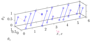
Figure 7: schematic domain of the multiscale embedding pde (5.4) for a field ${\mathfrak{u}}(t,{{\cal\mathchoice{\scriptstyle X}{\scriptstyle X}{\scriptscriptstyle X}{\scriptscriptstyle X}}},{\text{\boldmath$\theta$}})$, for ${{\cal\mathchoice{\scriptstyle X}{\scriptstyle X}{\scriptscriptstyle X}{\scriptscriptstyle X}}}\in{\mathbb{X}}\subset{\mathbb{R}}$ and for ${\text{\boldmath$\theta$}}\in\Theta:=[0,1]^{2}$. Here the periodicities $\ell_{1}=1.62$ and $\ell_{2}=0.72$ so ${\mathcal{E}}=\begin{bmatrix}1.62&0.72\end{bmatrix}$. We obtain solutions of the heterogeneous pde (5.1) on such blue lines as $u_{\text{\boldmath$\phi$}}(t,x):={\mathfrak{u}}(t,x,{\text{\boldmath$\phi$}}+{\mathcal{E}}^{+}x)$ for every constant phase ${\text{\boldmath$\phi$}}\in{\mathbb{R}}^{2}$, here ${\text{\boldmath$\phi$}}=(0.82,0.32)$, and where the third argument of $\mathfrak{u}$ has components modulo $1$.

As indicated by the schematic case illustrated in fig. 7, let’s create the desired phase-shift embedding by considering a field ${\mathfrak{u}}(t,{\text{\boldmath$\cal\mathchoice{\scriptstyle X}{\scriptstyle X}{\scriptscriptstyle X}{\scriptscriptstyle X}$}},{\text{\boldmath$\theta$}})$, implicitly depending on $z$, and satisfying the pde

$$\partial_{t}^{\alpha}{\mathfrak{u}} ={\mathcal{L}}({\text{\boldmath$\cal\mathchoice{\scriptstyle X}{\scriptstyle X}{\scriptscriptstyle X}{\scriptscriptstyle X}$}},{\text{\boldmath$\theta$}}){\mathfrak{u}}-(\text{\boldmath$\nabla$}_{\!\!{\text{\boldmath$\cal\mathchoice{\scriptstyle X}{\scriptstyle X}{\scriptscriptstyle X}{\scriptscriptstyle X}$}}}^{T}+\text{\boldmath$\nabla$}_{\!\!{\text{\boldmath$\theta$}}}^{T}{\mathcal{E}}^{+}){\text{\boldmath$f$}}\big{(}{\text{\boldmath$\cal\mathchoice{\scriptstyle X}{\scriptstyle X}{\scriptscriptstyle X}{\scriptscriptstyle X}$}},{\text{\boldmath$\theta$}},{\mathfrak{u}},{\mathfrak{u}}_{\text{\boldmath$\cal\mathchoice{\scriptstyle X}{\scriptstyle X}{\scriptscriptstyle X}{\scriptscriptstyle X}$}}+{\mathcal{E}}^{+T}{\mathfrak{u}}_{\text{\boldmath$\theta$}}\big{)}$$

$$\quad{}+\gamma g\big{(}t,{\text{\boldmath$\cal\mathchoice{\scriptstyle X}{\scriptstyle X}{\scriptscriptstyle X}{\scriptscriptstyle X}$}},{\text{\boldmath$\theta$}},{\mathfrak{u}},{\mathfrak{u}}_{\text{\boldmath$\cal\mathchoice{\scriptstyle X}{\scriptstyle X}{\scriptscriptstyle X}{\scriptscriptstyle X}$}}+{\mathcal{E}}^{+T}{\mathfrak{u}}_{\text{\boldmath$\theta$}}\big{)},$$ (5.4)

in the domain ${\mathbb{D}}:={\mathbb{X}}\times\Theta\times{\mathbb{Z}}$ for the unit $P$-cube $\Theta:=[0,1]^{P}$, and with boundary conditions of $1$-periodicity in $\theta_{p}$. The subscripts $\cal\mathchoice{\scriptstyle X}{\scriptstyle X}{\scriptscriptstyle X}{\scriptscriptstyle X}$ and $\theta$ denote the respective gradient operator, that is, ${\mathfrak{u}}_{\text{\boldmath$\cal\mathchoice{\scriptstyle X}{\scriptstyle X}{\scriptscriptstyle X}{\scriptscriptstyle X}$}}:=\text{\boldmath$\nabla$}_{\!\!{\text{\boldmath$\cal\mathchoice{\scriptstyle X}{\scriptstyle X}{\scriptscriptstyle X}{\scriptscriptstyle X}$}}}{\mathfrak{u}}$ and ${\mathfrak{u}}_{\text{\boldmath$\theta$}}:=\text{\boldmath$\nabla$}_{\!\!{\text{\boldmath$\theta$}}}{\mathfrak{u}}$ . We assume that the heterogeneous explicit dependence upon ${\text{\boldmath$\cal\mathchoice{\scriptstyle X}{\scriptstyle X}{\scriptscriptstyle X}{\scriptscriptstyle X}$}},{\text{\boldmath$\theta$}}$ in ${\mathcal{L}}\mathchar 8507\relax{}{\text{\boldmath$f$}}\mathchar 8507\relax{}g$ are regular enough that general solutions $\mathfrak{u}$ of pde eq. 5.4 are in ${\mathbb{H}}^{N}_{\mathbb{D}}:=W^{(N+1,2),p}({\mathbb{X}}\times\Theta)\times{\mathbb{H}}_{\mathbb{Z}}$ for some chosen order $N$. The domain $\mathbb{D}$ (fig. 7) is multiscale as it is large in $\cal\mathchoice{\scriptstyle X}{\scriptstyle X}{\scriptscriptstyle X}{\scriptscriptstyle X}$, and relatively thin in both $z$ and $\theta$. I emphasise that this domain has finite aspect ratio: we do not take any limit involving an aspect ratio tending to zero nor to infinity.

fig. 7 indicates that we regard ${\text{\boldmath$\cal\mathchoice{\scriptstyle X}{\scriptstyle X}{\scriptscriptstyle X}{\scriptscriptstyle X}$}}={\text{\boldmath$x$}}$ . The distinction between $\cal\mathchoice{\scriptstyle X}{\scriptstyle X}{\scriptscriptstyle X}{\scriptscriptstyle X}$ and $x$ is that partial derivatives in $\cal\mathchoice{\scriptstyle X}{\scriptstyle X}{\scriptscriptstyle X}{\scriptscriptstyle X}$ are done keeping $\theta$ constant (e.g., parallel to the $\cal\mathchoice{\scriptstyle X}{\scriptstyle X}{\scriptscriptstyle X}{\scriptscriptstyle X}$-axis in fig. 7), whereas partial derivatives in $x$ are done keeping the phase-shift $\phi$ constant (e.g., along the (blue) diagonal lines in fig. 7).

Lemma 5.

For every smooth solution ${\mathfrak{u}}(t,{\text{\boldmath$\cal\mathchoice{\scriptstyle X}{\scriptstyle X}{\scriptscriptstyle X}{\scriptscriptstyle X}$}},{\text{\boldmath$\theta$}})\in{\mathbb{H}}^{N}_{\mathbb{D}}$ of the embedding pde (5.4), and for every vector of phases $\phi$, the field $u_{\text{\boldmath$\phi$}}(t,{\text{\boldmath$x$}}):={\mathfrak{u}}(t,{\text{\boldmath$x$}},{\text{\boldmath$\phi$}}+{\mathcal{E}}^{+}{\text{\boldmath$x$}})$ (for example, the field ${\mathfrak{u}}$ evaluated on the solid-blue lines in fig. 7) is in the Sobolov space $W^{2,2}({\mathbb{X}})\times{\mathbb{H}}_{\mathbb{Z}}$ , and satisfies the heterogeneous, phase-shifted, pde

$$\partial_{t}^{\alpha}{u_{\text{\boldmath$\phi$}}} ={\mathcal{L}}({\text{\boldmath$x$}},{\text{\boldmath$\phi$}}+{\mathcal{E}}^{+}{\text{\boldmath$x$}})u_{\text{\boldmath$\phi$}}-\text{\boldmath$\nabla$}^{T}{\text{\boldmath$f$}}({\text{\boldmath$x$}},{\text{\boldmath$\phi$}}+{\mathcal{E}}^{+}{\text{\boldmath$x$}},u_{\text{\boldmath$\phi$}},\text{\boldmath$\nabla$}u_{\text{\boldmath$\phi$}})$$

$$\quad{}+\gamma g(t,{\text{\boldmath$x$}},{\text{\boldmath$\phi$}}+{\mathcal{E}}^{+}{\text{\boldmath$x$}},u_{\text{\boldmath$\phi$}},\text{\boldmath$\nabla$}u_{\text{\boldmath$\phi$}}).$$ (5.5)

Hence $u_{\text{\boldmath$0$}}(t,{\text{\boldmath$x$}}):={\mathfrak{u}}(t,{\text{\boldmath$x$}},{\mathcal{E}}^{+}{\text{\boldmath$x$}})$ satisfies the given heterogeneous pde (5.1).

Recall that the most common boundary conditions assumed for rves are periodic, although in the usual homogenization arguments other boundary conditions appear equally as valid despite giving slightly different results (e.g., Mercer et al. 2015). In contrast, here the boundary conditions of $1$-periodicity in microscale $\theta$ are not assumed but instead arise naturally due to the ensemble of phase-shifts. That is, what in other approaches has to be assumed, in this approach arises naturally.

Proof.

Start by considering the left-hand side of pde (5.5), namely the time evolution operator

$$\partial_{t}^{\alpha}{u_{\text{\boldmath$\phi$}}} =\partial_{t}^{\alpha}{}{\mathfrak{u}}(t,{\text{\boldmath$x$}},{\text{\boldmath$\phi$}}+{\mathcal{E}}^{+}{\text{\boldmath$x$}})$$

$$=\left[\partial_{t}^{\alpha}{\mathfrak{u}}\right]_{(t,{\text{\boldmath$x$}},{\text{\boldmath$\phi$}}+{\mathcal{E}}^{+}{\text{\boldmath$x$}})}\qquad\text{(which by {pde}~{}\eqref{Eempde} becomes)}$$

$$=\left[{\mathcal{L}}{\mathfrak{u}}-(\text{\boldmath$\nabla$}_{\!\!{\text{\boldmath$\cal\mathchoice{\scriptstyle X}{\scriptstyle X}{\scriptscriptstyle X}{\scriptscriptstyle X}$}}}^{T}+\text{\boldmath$\nabla$}_{\!\!{\text{\boldmath$\theta$}}}^{T}{\mathcal{E}}^{+}){\text{\boldmath$f$}}({\text{\boldmath$\cal\mathchoice{\scriptstyle X}{\scriptstyle X}{\scriptscriptstyle X}{\scriptscriptstyle X}$}},{\text{\boldmath$\theta$}},{\mathfrak{u}},{\mathfrak{u}}_{\text{\boldmath$\cal\mathchoice{\scriptstyle X}{\scriptstyle X}{\scriptscriptstyle X}{\scriptscriptstyle X}$}}+{\mathcal{E}}^{+T}{\mathfrak{u}}_{\text{\boldmath$\theta$}})\right.$$

$$\qquad\left.{}+\gamma g(t,{\text{\boldmath$\cal\mathchoice{\scriptstyle X}{\scriptstyle X}{\scriptscriptstyle X}{\scriptscriptstyle X}$}},{\text{\boldmath$\theta$}},{\mathfrak{u}},{\mathfrak{u}}_{\text{\boldmath$\cal\mathchoice{\scriptstyle X}{\scriptstyle X}{\scriptscriptstyle X}{\scriptscriptstyle X}$}}+{\mathcal{E}}^{+T}{\mathfrak{u}}_{\text{\boldmath$\theta$}})\right]_{(t,{\text{\boldmath$x$}},{\text{\boldmath$\phi$}}+{\mathcal{E}}^{+}{\text{\boldmath$x$}})}$$

$$=\left[{\mathcal{L}}({\text{\boldmath$\cal\mathchoice{\scriptstyle X}{\scriptstyle X}{\scriptscriptstyle X}{\scriptscriptstyle X}$}},{\text{\boldmath$\theta$}}){\mathfrak{u}}\right]_{(t,{\text{\boldmath$x$}},{\text{\boldmath$\phi$}}+{\mathcal{E}}^{+}{\text{\boldmath$x$}})}-\text{\boldmath$\nabla$}^{T}\left\{\left[{\text{\boldmath$f$}}({\text{\boldmath$\cal\mathchoice{\scriptstyle X}{\scriptstyle X}{\scriptscriptstyle X}{\scriptscriptstyle X}$}},{\text{\boldmath$\theta$}},{\mathfrak{u}},{\mathfrak{u}}_{\text{\boldmath$\cal\mathchoice{\scriptstyle X}{\scriptstyle X}{\scriptscriptstyle X}{\scriptscriptstyle X}$}}+{\mathcal{E}}^{+T}{\mathfrak{u}}_{\text{\boldmath$\theta$}})\right]_{(t,{\text{\boldmath$x$}},{\text{\boldmath$\phi$}}+{\mathcal{E}}^{+}{\text{\boldmath$x$}})}\right\}$$

$$\qquad{}+\gamma g(t,{\text{\boldmath$x$}},{\text{\boldmath$x$}}+{\text{\boldmath$\phi$}},u_{\text{\boldmath$\phi$}},\text{\boldmath$\nabla$}u_{\text{\boldmath$\phi$}})$$

$$={\mathcal{L}}({\text{\boldmath$x$}},{\text{\boldmath$\phi$}}+{\mathcal{E}}^{+}{\text{\boldmath$x$}})u_{\text{\boldmath$\phi$}}-\text{\boldmath$\nabla$}^{T}{\text{\boldmath$f$}}({\text{\boldmath$x$}},{\text{\boldmath$\phi$}}+{\mathcal{E}}^{+}{\text{\boldmath$x$}},u_{\text{\boldmath$\phi$}},\text{\boldmath$\nabla$}u_{\text{\boldmath$\phi$}})$$

$$\qquad{}+\gamma g(t,{\text{\boldmath$x$}},{\text{\boldmath$\phi$}}+{\mathcal{E}}^{+}{\text{\boldmath$x$}},u_{\text{\boldmath$\phi$}},\text{\boldmath$\nabla$}u_{\text{\boldmath$\phi$}}),$$

namely the right-hand side of (5.5). Hence, provided pde (5.4) has boundary conditions of $1$-periodicity in $\theta_{p}$, every solution of the embedding pde (5.4) gives a solution of the original pde (5.1) for every $P$-dimensional phase-shift $\phi$ of the heterogeneity.

In particular, the field $u_{\text{\boldmath$0$}}(t,{\text{\boldmath$x$}})$, of phase-shift ${\text{\boldmath$\phi$}}=\text{\boldmath$0$}$, satisfies the given heterogeneous pde (5.1). ∎

Lemma 6 (converse).

Suppose we have a family of solutions $u_{\text{\boldmath$\phi$}}(t,{\text{\boldmath$x$}})$ of the phase-shifted pde (5.5)—a family parametrised by the phase vector ${\text{\boldmath$\phi$}}\in{\mathbb{R}}^{p}$—and the family depends smoothly enough upon $t,{\text{\boldmath$x$}},{\text{\boldmath$\phi$}}$ that the following ${\mathfrak{u}}\in{\mathbb{H}}^{N}_{\mathbb{D}}$. Then the field ${\mathfrak{u}}(t,{\text{\boldmath$\cal\mathchoice{\scriptstyle X}{\scriptstyle X}{\scriptscriptstyle X}{\scriptscriptstyle X}$}},{\text{\boldmath$\theta$}}):=u_{{\text{\boldmath$\theta$}}-{\mathcal{E}}^{+}{\text{\boldmath$\cal\mathchoice{\scriptstyle X}{\scriptstyle X}{\scriptscriptstyle X}{\scriptscriptstyle X}$}}}(t,{\text{\boldmath$\cal\mathchoice{\scriptstyle X}{\scriptstyle X}{\scriptscriptstyle X}{\scriptscriptstyle X}$}})$ satisfies the embedding pde (5.4).

Proof.

First, from the pde (5.4), consider

$${\mathfrak{u}}_{\text{\boldmath$\cal\mathchoice{\scriptstyle X}{\scriptstyle X}{\scriptscriptstyle X}{\scriptscriptstyle X}$}}+{\mathcal{E}}^{+T}{\mathfrak{u}}_{\text{\boldmath$\theta$}} =\left[(-{\mathcal{E}}^{+})^{T}\mathchoice{\frac{\partial u_{\text{\boldmath$\phi$}}}{\partial{\text{\boldmath$\phi$}}}}{{\partial u_{\text{\boldmath$\phi$}}}/{\partial{\text{\boldmath$\phi$}}}}{{\partial u_{\text{\boldmath$\phi$}}}/{\partial{\text{\boldmath$\phi$}}}}{{\partial u_{\text{\boldmath$\phi$}}}/{\partial{\text{\boldmath$\phi$}}}}+\mathchoice{\frac{\partial u_{\text{\boldmath$\phi$}}}{\partial{\text{\boldmath$x$}}}}{{\partial u_{\text{\boldmath$\phi$}}}/{\partial{\text{\boldmath$x$}}}}{{\partial u_{\text{\boldmath$\phi$}}}/{\partial{\text{\boldmath$x$}}}}{{\partial u_{\text{\boldmath$\phi$}}}/{\partial{\text{\boldmath$x$}}}}+{\mathcal{E}}^{+T}\mathchoice{\frac{\partial u_{\text{\boldmath$\phi$}}}{\partial{\text{\boldmath$\phi$}}}}{{\partial u_{\text{\boldmath$\phi$}}}/{\partial{\text{\boldmath$\phi$}}}}{{\partial u_{\text{\boldmath$\phi$}}}/{\partial{\text{\boldmath$\phi$}}}}{{\partial u_{\text{\boldmath$\phi$}}}/{\partial{\text{\boldmath$\phi$}}}}\right]_{{\text{\boldmath$\phi$}}={\text{\boldmath$\theta$}}-{\mathcal{E}}^{+}{\text{\boldmath$\cal\mathchoice{\scriptstyle X}{\scriptstyle X}{\scriptscriptstyle X}{\scriptscriptstyle X}$}},{\text{\boldmath$x$}}={\text{\boldmath$\cal\mathchoice{\scriptstyle X}{\scriptstyle X}{\scriptscriptstyle X}{\scriptscriptstyle X}$}}}$$

$$=\big{[}\text{\boldmath$\nabla$}{u_{\text{\boldmath$\phi$}}}\big{]}_{{\text{\boldmath$\phi$}}={\text{\boldmath$\theta$}}-{\mathcal{E}}^{+}{\text{\boldmath$\cal\mathchoice{\scriptstyle X}{\scriptstyle X}{\scriptscriptstyle X}{\scriptscriptstyle X}$}},{\text{\boldmath$x$}}={\text{\boldmath$\cal\mathchoice{\scriptstyle X}{\scriptstyle X}{\scriptscriptstyle X}{\scriptscriptstyle X}$}}}\,.$$

Second, since ${\text{\boldmath$\phi$}}={\text{\boldmath$\theta$}}-{\mathcal{E}}^{+}{\text{\boldmath$\cal\mathchoice{\scriptstyle X}{\scriptstyle X}{\scriptscriptstyle X}{\scriptscriptstyle X}$}}={\text{\boldmath$\theta$}}-{\mathcal{E}}^{+}{\text{\boldmath$x$}}$ , that is ${\text{\boldmath$\theta$}}={\text{\boldmath$\phi$}}+{\mathcal{E}}^{+}{\text{\boldmath$x$}}$ , then for every smooth ${\text{\boldmath$f$}}({\text{\boldmath$\cal\mathchoice{\scriptstyle X}{\scriptstyle X}{\scriptscriptstyle X}{\scriptscriptstyle X}$}},{\text{\boldmath$\theta$}})$, $(\text{\boldmath$\nabla$}_{\!\!{\text{\boldmath$\cal\mathchoice{\scriptstyle X}{\scriptstyle X}{\scriptscriptstyle X}{\scriptscriptstyle X}$}}}^{T}+\text{\boldmath$\nabla$}_{\!\!{\text{\boldmath$\theta$}}}^{T}{\mathcal{E}}^{+}){\text{\boldmath$f$}}=\text{\boldmath$\nabla$}^{T}\big{\{}f|_{{\text{\boldmath$\cal\mathchoice{\scriptstyle X}{\scriptstyle X}{\scriptscriptstyle X}{\scriptscriptstyle X}$}}={\text{\boldmath$x$}},{\text{\boldmath$\theta$}}={\text{\boldmath$\phi$}}+{\mathcal{E}}^{+}{\text{\boldmath$x$}}}\big{\}}$. Thirdly, hence the right-hand-side of pde (5.4) becomes

$${\mathcal{L}}({\text{\boldmath$\cal\mathchoice{\scriptstyle X}{\scriptstyle X}{\scriptscriptstyle X}{\scriptscriptstyle X}$}},{\text{\boldmath$\theta$}}){\mathfrak{u}}-(\text{\boldmath$\nabla$}_{\!\!{\text{\boldmath$\cal\mathchoice{\scriptstyle X}{\scriptstyle X}{\scriptscriptstyle X}{\scriptscriptstyle X}$}}}^{T}+\text{\boldmath$\nabla$}_{\!\!{\text{\boldmath$\theta$}}}^{T}{\mathcal{E}}^{+}){\text{\boldmath$f$}}({\text{\boldmath$\cal\mathchoice{\scriptstyle X}{\scriptstyle X}{\scriptscriptstyle X}{\scriptscriptstyle X}$}},{\text{\boldmath$\theta$}},{\mathfrak{u}},{\mathfrak{u}}_{\text{\boldmath$\cal\mathchoice{\scriptstyle X}{\scriptstyle X}{\scriptscriptstyle X}{\scriptscriptstyle X}$}}+{\mathcal{E}}^{+T}{\mathfrak{u}}_{\text{\boldmath$\theta$}})$$

$$\qquad{}+\gamma g(t,{\text{\boldmath$\cal\mathchoice{\scriptstyle X}{\scriptstyle X}{\scriptscriptstyle X}{\scriptscriptstyle X}$}},{\text{\boldmath$\theta$}},{\mathfrak{u}},{\mathfrak{u}}_{\text{\boldmath$\cal\mathchoice{\scriptstyle X}{\scriptstyle X}{\scriptscriptstyle X}{\scriptscriptstyle X}$}}+{\mathcal{E}}^{+T}{\mathfrak{u}}_{\text{\boldmath$\theta$}})$$

$$=\big{[}{\mathcal{L}}({\text{\boldmath$\cal\mathchoice{\scriptstyle X}{\scriptstyle X}{\scriptscriptstyle X}{\scriptscriptstyle X}$}},{\text{\boldmath$\theta$}}){\mathfrak{u}}\big{]}|_{{\text{\boldmath$\cal\mathchoice{\scriptstyle X}{\scriptstyle X}{\scriptscriptstyle X}{\scriptscriptstyle X}$}}={\text{\boldmath$x$}},{\text{\boldmath$\theta$}}={\text{\boldmath$\phi$}}+{\mathcal{E}}^{+}{\text{\boldmath$x$}}}-\text{\boldmath$\nabla$}^{T}\big{\{}{\text{\boldmath$f$}}({\text{\boldmath$\cal\mathchoice{\scriptstyle X}{\scriptstyle X}{\scriptscriptstyle X}{\scriptscriptstyle X}$}},{\text{\boldmath$\theta$}},{\mathfrak{u}},{\mathfrak{u}}_{\text{\boldmath$\cal\mathchoice{\scriptstyle X}{\scriptstyle X}{\scriptscriptstyle X}{\scriptscriptstyle X}$}}+{\mathcal{E}}^{+T}{\mathfrak{u}}_{\text{\boldmath$\theta$}})|_{{\text{\boldmath$\cal\mathchoice{\scriptstyle X}{\scriptstyle X}{\scriptscriptstyle X}{\scriptscriptstyle X}$}}={\text{\boldmath$x$}},{\text{\boldmath$\theta$}}={\text{\boldmath$\phi$}}+{\mathcal{E}}^{+}{\text{\boldmath$x$}}}\big{\}}$$

$$\qquad{}+\gamma g(t,{\text{\boldmath$\cal\mathchoice{\scriptstyle X}{\scriptstyle X}{\scriptscriptstyle X}{\scriptscriptstyle X}$}},{\text{\boldmath$\theta$}},{\mathfrak{u}},{\mathfrak{u}}_{\text{\boldmath$\cal\mathchoice{\scriptstyle X}{\scriptstyle X}{\scriptscriptstyle X}{\scriptscriptstyle X}$}}+{\mathcal{E}}^{+T}{\mathfrak{u}}_{\text{\boldmath$\theta$}})|_{{\text{\boldmath$\cal\mathchoice{\scriptstyle X}{\scriptstyle X}{\scriptscriptstyle X}{\scriptscriptstyle X}$}}={\text{\boldmath$x$}},{\text{\boldmath$\theta$}}={\text{\boldmath$\phi$}}+{\mathcal{E}}^{+}{\text{\boldmath$x$}}}$$

$$={\mathcal{L}}({\text{\boldmath$x$}},{\text{\boldmath$\phi$}}+{\mathcal{E}}^{+}{\text{\boldmath$x$}})u_{\text{\boldmath$\phi$}}-\text{\boldmath$\nabla$}^{T}{\text{\boldmath$f$}}({\text{\boldmath$x$}},{\text{\boldmath$\phi$}}+{\mathcal{E}}^{+}{\text{\boldmath$x$}},u_{\text{\boldmath$\phi$}},\text{\boldmath$\nabla$}u_{\text{\boldmath$\phi$}})$$

$$\qquad{}+\gamma g(t,{\text{\boldmath$x$}},{\text{\boldmath$\phi$}}+{\mathcal{E}}^{+}{\text{\boldmath$x$}},u_{\text{\boldmath$\phi$}},\text{\boldmath$\nabla$}u_{\text{\boldmath$\phi$}})\,,$$

the right-hand side of pde (5.5). Lastly, since $\partial_{t}^{\alpha}{\mathfrak{u}}(t,{\text{\boldmath$\cal\mathchoice{\scriptstyle X}{\scriptstyle X}{\scriptscriptstyle X}{\scriptscriptstyle X}$}},{\text{\boldmath$\theta$}})=\partial_{t}^{\alpha}{u_{{\text{\boldmath$\theta$}}-{\mathcal{E}}^{+}{\text{\boldmath$\cal\mathchoice{\scriptstyle X}{\scriptstyle X}{\scriptscriptstyle X}{\scriptscriptstyle X}$}}}}$ it follows that ${\mathfrak{u}}:=u_{{\text{\boldmath$\theta$}}-{\mathcal{E}}^{+}{\text{\boldmath$\cal\mathchoice{\scriptstyle X}{\scriptstyle X}{\scriptscriptstyle X}{\scriptscriptstyle X}$}}}(t,{\text{\boldmath$\cal\mathchoice{\scriptstyle X}{\scriptstyle X}{\scriptscriptstyle X}{\scriptscriptstyle X}$}})$ satisfies the embedding pde (5.4). ∎

Consequently, pdes (LABEL:Eempde,Egenpde) are equivalent, and they may provide us with an ensemble of solutions for an ensemble of materials all with the same heterogeneity structure, but with the structural phase of the material shifted through all possible phases. The key difference between pdes eqs. 5.1 and 5.4 is that although pde (5.1) is heterogeneous in space $x$, the embedding pde (5.4) is homogeneous in space $\cal\mathchoice{\scriptstyle X}{\scriptstyle X}{\scriptscriptstyle X}{\scriptscriptstyle X}$. Because of this homogeneity, section 5.2 is empowered to apply an existing rigorous theory for slow variations in space that leads to desired multi-continuum homogenisations of the pde eq. 5.4, and hence to that of (5.1).

5.2 Invariant manifolds of multi-continuum, micromorphic, any-order homogenization

Generalising section 2.2, let’s analyse the embedding pde (5.4) for useful ‘homogenized’ invariant manifolds. Such invariant manifolds are to express and support the relevance of a potential hierarchy of accurate homogenizations for the original heterogeneous pde (5.1). The systematic approach developed simplifies considerably much of the “difficulty to choose a priori an appropriate model for a given microstructure” discussed by Alavi et al. (2023) [p.2164].

Developments in dynamical systems theory inspired by earlier more formal arguments establishes how to construct a pde model for the macroscale spatial structure of pde solutions in multiscale domains $\mathbb{D}$ such as fig. 7. The technique is to base analysis on the case where variations in $\cal\mathchoice{\scriptstyle X}{\scriptstyle X}{\scriptscriptstyle X}{\scriptscriptstyle X}$ are over a large enough scale that they are approximately negligible—the variations are both directly in the parametric $\cal\mathchoice{\scriptstyle X}{\scriptstyle X}{\scriptscriptstyle X}{\scriptscriptstyle X}$ dependence of ${\mathcal{L}}\mathchar 8507\relax{}{\text{\boldmath$f$}}\mathchar 8507\relax{}g$ and indirectly via the field ${\mathfrak{u}}$. Then we treat finite, macroscale, variations in $\cal\mathchoice{\scriptstyle X}{\scriptstyle X}{\scriptscriptstyle X}{\scriptscriptstyle X}$ as a regular perturbation. Despite the derivative $\partial_{\text{\boldmath$\cal\mathchoice{\scriptstyle X}{\scriptstyle X}{\scriptscriptstyle X}{\scriptscriptstyle X}$}}$ being an unbounded operator, the theoretical developments justify being able to treat such derivatives as ‘small’ (e.g., Roberts & Bunder 2017, p.987). Hence the perturbation analysis proceeds to any chosen order $N$ in the ‘small’ derivatives $\partial_{\text{\boldmath$\cal\mathchoice{\scriptstyle X}{\scriptstyle X}{\scriptscriptstyle X}{\scriptscriptstyle X}$}}$ with quantifiable remainder error (Roberts & Bunder 2017, (52)).

For two examples in linear elasticity systems, the usual leading order homogenizations are the case $N=2$, and the so-called second-order homogenizations correspond to the higher-order $N=4$. Because of the power of the established dynamical system framework, here we allow arbitrary order $N$.

5.2.1 Linear basis of invariant manifolds

Invariant manifolds are mostly constructed from the base of an equilibrium or a family of equilibria, as we do here to generalise section 2.2. In the vicinity of each and every equilibria we characterise all solutions in terms of spectral properties of the system’s linearisation. Consequently, we then construct relevant invariant manifolds that pass through the base equilibria and extend into the state space. The correspondingly constructed evolution then forms a closed accurate macroscale homogenization.

Equilibria

Following Bunder & Roberts (2021) we consider the dynamics of the embedding pde eq. 5.4 in a mesoscale locale of each and every ‘cross-section’ position ${\text{\boldmath$\cal\mathchoice{\scriptstyle X}{\scriptstyle X}{\scriptscriptstyle X}{\scriptscriptstyle X}$}}={\text{\boldmath$X$}}\in{\mathbb{X}}$ of interest in the physical problem at hand. In such a mesoscale locale the variations in macroscale variable $\cal\mathchoice{\scriptstyle X}{\scriptstyle X}{\scriptscriptstyle X}{\scriptscriptstyle X}$ are small enough so that for linearisation purposes we consider the macroscale gradients negligible, $\text{\boldmath$\nabla$}_{\!\!{\text{\boldmath$\cal\mathchoice{\scriptstyle X}{\scriptstyle X}{\scriptscriptstyle X}{\scriptscriptstyle X}$}}}\equiv 0$. Many secondary physical nonlinearities or forcing effects are gathered into $g(t,{\text{\boldmath$\cal\mathchoice{\scriptstyle X}{\scriptstyle X}{\scriptscriptstyle X}{\scriptscriptstyle X}$}},{\text{\boldmath$\theta$}},{\mathfrak{u}},{\mathfrak{u}}_{\text{\boldmath$\cal\mathchoice{\scriptstyle X}{\scriptstyle X}{\scriptscriptstyle X}{\scriptscriptstyle X}$}}+{\mathfrak{u}}_{\text{\boldmath$\theta$}})$, multiplied by perturbation parameter $\gamma$, so we seek equilibria that requires the coefficient $\gamma=0$ . That invariant manifold theory supports modelling in the vicinity of each equilibria empowers us to systematically and accurately model effects with non-zero gradients $\text{\boldmath$\nabla$}_{\!\!{\text{\boldmath$\cal\mathchoice{\scriptstyle X}{\scriptstyle X}{\scriptscriptstyle X}{\scriptscriptstyle X}$}}}$, non-zero $\gamma$, and from nonlinearities.

With effectively zero $\text{\boldmath$\nabla$}_{\!\!{\text{\boldmath$\cal\mathchoice{\scriptstyle X}{\scriptstyle X}{\scriptscriptstyle X}{\scriptscriptstyle X}$}}}$ and zero $\gamma$ the dynamics of the embedding pde eq. 5.4 in the locale near $X$ reduces to the cross-sectional, cell-problem

$$\partial_{t}^{\alpha}{\mathfrak{u}}={\mathcal{L}}({\text{\boldmath$X$}},{\text{\boldmath$\theta$}}){\mathfrak{u}}-\text{\boldmath$\nabla$}_{\!\!{\text{\boldmath$\theta$}}}^{T}{\text{\boldmath$f$}}({\text{\boldmath$X$}},{\text{\boldmath$\theta$}},{\mathfrak{u}},{\mathcal{E}}^{+T}{\mathfrak{u}}_{\text{\boldmath$\theta$}}),$$ (5.6)

for $1$-periodicity in $\theta_{p}$, and at every cross-section ${\text{\boldmath$X$}}\in{\mathbb{X}}$ of interest. For each $X$, the cross-sectional pde eq. 5.6 is a cell-problem in that it only contains dependence upon $\theta$ and implicitly $z$. The following treatment of pde eq. 5.6 is parametrised by the macroscale locale $X$, and so many of the quantities identified may depend upon $X$, as in functionally graded materials, although often not. For brevity, any such $X$-dependence is mostly implicit in the following.

We assume that the cell-problem eq. 5.6 has one or more chosen equilibria ${\mathfrak{u}}={\mathfrak{u}}^{*}({\text{\boldmath$\theta$}})\in{\mathbb{H}}_{\Theta}\times{\mathbb{H}}_{\mathbb{Z}}$. Often these equilibria will zero the flux $f$. Often the equilibria ${\mathfrak{u}}^{*}$ are constant in $\theta$ and in $z$: but, they need not be constant. Often the chosen equilibria form a subspace such as ${\mathfrak{u}}^{*}\propto v_{0}({\text{\boldmath$\theta$}})$ for some $v_{0}$. Define ${\mathbb{E}}:=\{\text{chosen equilibria }{\mathfrak{u}}^{*}\}\subset{\mathbb{H}}_{\Theta}\times{\mathbb{H}}_{\mathbb{Z}}$. That is, ${\mathcal{L}}{\mathfrak{u}}^{*}-\text{\boldmath$\nabla$}_{\!\!{\text{\boldmath$\theta$}}}^{T}{\text{\boldmath$f$}}({\text{\boldmath$X$}},{\text{\boldmath$\theta$}},{\mathfrak{u}}^{*},{\mathcal{E}}^{+T}{\mathfrak{u}}^{*}_{\text{\boldmath$\theta$}})=0$ for every ${\mathfrak{u}}^{*}\in{\mathbb{E}}$.

In application, one often has useful physical intuition about a suitable base set of equilibria $\mathbb{E}$ for the scenarios of interest. One then introduces the artificial ordering parameter $\gamma$ into the governing equations so that ${\mathcal{L}}{\mathfrak{u}}+\text{\boldmath$\nabla$}_{\!\!{\text{\boldmath$\theta$}}}^{T}{\text{\boldmath$f$}}$ has the desired equilibria $\mathbb{E}$, and all other terms are gathered into $\gamma g$ (e.g., Roberts 2015b, §9.1 and Part V). The systematic framework here empowers arbitrary order construction in such an artificial $\gamma$ (section 5.3) to enable reasonable prediction at the physically relevant $\gamma$ (usually at $\gamma=1$).

Characterise nearby dynamics via linearisation

For each ${\mathfrak{u}}^{*}\in{\mathbb{E}}$, explore the nearby dynamics by seeking solutions to the cell-problem eq. 5.6 in the form ${\mathfrak{u}}={\mathfrak{u}}^{*}({\text{\boldmath$\theta$}})+\hat{}{\mathfrak{u}}(t,{\text{\boldmath$\theta$}})$ for small $\hat{}{\mathfrak{u}}$. Then, invoking Frechet derivatives, the flux becomes

$$f ={\text{\boldmath$f$}}({\text{\boldmath$X$}},{\text{\boldmath$\theta$}},{\mathfrak{u}}^{*}+\hat{}{\mathfrak{u}},{\mathfrak{u}}^{*}_{\text{\boldmath$\theta$}}+\hat{}{\mathfrak{u}}_{\text{\boldmath$\theta$}})$$

$$\approx{\text{\boldmath$f$}}({\text{\boldmath$X$}},{\text{\boldmath$\theta$}},{\mathfrak{u}}^{*},{\mathfrak{u}}^{*}_{\text{\boldmath$\theta$}})+\underbrace{\mathchoice{\frac{\partial{\text{\boldmath$f$}}}{\partial{\mathfrak{u}}}}{{\partial{\text{\boldmath$f$}}}/{\partial{\mathfrak{u}}}}{{\partial{\text{\boldmath$f$}}}/{\partial{\mathfrak{u}}}}{{\partial{\text{\boldmath$f$}}}/{\partial{\mathfrak{u}}}}({\text{\boldmath$X$}},{\text{\boldmath$\theta$}},{\mathfrak{u}}^{*},{\mathfrak{u}}^{*}_{\text{\boldmath$\theta$}})}_{{}=:{\text{\boldmath$\jmath$}}^{*}({\text{\boldmath$X$}},y)}\hat{}{\mathfrak{u}}+\underbrace{\mathchoice{\frac{\partial{\text{\boldmath$f$}}}{\partial{\mathfrak{u}}_{\text{\boldmath$\theta$}}}}{{\partial{\text{\boldmath$f$}}}/{\partial{\mathfrak{u}}_{\text{\boldmath$\theta$}}}}{{\partial{\text{\boldmath$f$}}}/{\partial{\mathfrak{u}}_{\text{\boldmath$\theta$}}}}{{\partial{\text{\boldmath$f$}}}/{\partial{\mathfrak{u}}_{\text{\boldmath$\theta$}}}}({\text{\boldmath$X$}},{\text{\boldmath$\theta$}},{\mathfrak{u}}^{*},{\mathfrak{u}}^{*}_{\text{\boldmath$\theta$}})}_{{}=:J^{*}({\text{\boldmath$X$}},{\text{\boldmath$\theta$}})}\hat{}{\mathfrak{u}}_{\text{\boldmath$\theta$}}\,.$$

To characterise general solutions to the nearby dynamics we thus address the cell eigen-problem

$$\lambda v={\mathfrak{L}}v\,,\quad\text{where }{\mathfrak{L}}v:={\mathcal{L}}v-\text{\boldmath$\nabla$}_{\!\!{\text{\boldmath$\theta$}}}^{T}({\text{\boldmath$\jmath$}}^{*}v+J^{*}v_{\text{\boldmath$\theta$}}),\quad 1\text{-periodic in }\theta_{p},$$ (5.7)

for cell eigenvalues $\lambda$ and cell eigenfunctions $v({\text{\boldmath$\theta$}})$. Often the set $\mathbb{E}$ is chosen so that the cell-problem is independent of the equilibria ${\mathfrak{u}}^{*}\in{\mathbb{E}}$ .

Assumption 7 (eigenfunction decomposition).

Firstly, assume that non-empty $\mathbb{X}$,$\mathbb{E}$ exist where for every cross-section ${\text{\boldmath$X$}}\in{\mathbb{X}}$ and every equilibrium ${\mathfrak{u}}^{*}\in{\mathbb{E}}$, there exists for the cell eigen-problem eq. 5.7 a complete countable set of (generalised) eigenfunctions $v_{m}({\text{\boldmath$\theta$}})$ for corresponding eigenvalues $\lambda_{m}$ (sometimes complex valued), for index $m=0,1,2,\ldots$ (ordered so that $\Re\lambda_{m+1}\leq\Re\lambda_{m}$, and if $\Re\lambda_{m+1}=\Re\lambda_{m}$ then $\Im\lambda_{m+1}\leq\Im\lambda_{m}$). Secondly, assume that there exists a countable set of corresponding (generalised) adjoint eigenfunctions $w_{m}({\text{\boldmath$\theta$}})$ normalised so that $\left<w_{m},v_{m}\right>=\delta_{m,n}$ , such that the linear operator ${\mathfrak{L}}=\sum_{m=1}^{\infty}\lambda_{m}v_{m}\left<w_{m},\cdot\right>+\zeta_{m}v_{m}\left<w_{m+1},\cdot\right>$ in the space ${\mathbb{H}}_{\Theta\times{\mathbb{Z}}}$ (where $\zeta_{m}=0$ when $\lambda_{m}\neq\lambda_{m+1}$), and that ${\mathbb{H}}_{\Theta\times{\mathbb{Z}}}$ is the closure of absolutely convergent series for this decomposition of ${\mathfrak{L}}u$. Thirdly, assume these eigenfunctions and eigenvalues vary smoothly with macroscale ${\text{\boldmath$X$}}\in{\mathbb{X}}$.

Often the cell eigen-problem eq. 5.7 is independent of macroscale $X$. However, functionally graded materials that have graduations in a large space dimension are examples of $X$-dependence. If such a graded material has a sudden/step change in material properties, then such a change generates physical ‘boundary’ layers that have to be excised from the spatial domain $\mathbb{X}$. Such physical ‘boundary’ layers about a material change are instead resolved in the homogenisation via an argument akin to that for boundary conditions (e.g., Roberts 1992, Chen et al. 2018).

For each in $\mathbb{X}$ and $\mathbb{E}$, since the eigenfunctions are complete, a general solution to the linearised cell-problem eq. 5.6 is thus

$${\mathfrak{u}}={\mathfrak{u}}^{*}+\sum_{m=1}^{\infty}a_{m}(t)v_{m}({\text{\boldmath$\theta$}}),$$ (5.8a)

where $$a_{m}(t) m$$ is a general solution to the th-mode ode

$$\partial_{t}^{\alpha}a_{m}=\lambda_{m}a_{m}\,.$$ (5.8b)

Now the developing argument splits depending upon the nature of $\partial_{t}^{\alpha}$, the spectrum of eigenvalues $\{\lambda_{m}:m=0,1,2,\ldots\}$, and also upon external knowledge about the physical problem and its context. It is not feasible to address all the myriad of possibilities for the time evolution operator $\partial_{t}^{\alpha}$. Instead we focus mainly on the two main cases of first- and second-order time derivatives, $\alpha=1,2$, and discuss briefly other cases.

Perhaps use cells twice the minimum size

But before we leave the cell-problem, recall the material and deformation shown by fig. 1. In the un-deformed state, such as the left and right ends of the material as shown, the periodic heterogeneous cell is clearly a square, say with side length $\ell$, each microscale square with one circular inclusion. However, choosing such a cell results in homogenisations that are almost certainly unable to predict the checkerboard pattern in the middle of fig. 1—the macroscale variations would be too short for validity of the homogenisation. To encompass this checkerboard deformation one should instead aim for a square cell of size $2\ell\times 2\ell$ containing four inclusions; that is, embed the physical problem using heterogeneity period $2\ell$ in both directions. Then a local checkerboard pattern can be one of the sub-cell modes $v_{m}({\text{\boldmath$\theta$}})$ in a multi-continuum micromorphic homogenisation (e.g., Rokoš et al. 2019).

Combescure (2022) used cognate 1-D examples in discussing selecting generalized continuum models for materials displaying microstructure instabilities. Indeed, recall Mathieu’s equation for oscillations in $u(t)$ with parametric forcing, $u_{tt}+(\omega^{2}+\epsilon\cos t)u=0$ (e.g., Roberts 2015b, §3.7.1). This system has instabilities when the natural frequency $\omega=k/2$ for integer $k$. The strongest instability is when $\omega=1/2$, that is, at twice the period of the forcing. The spatial analogue for homogenisation is that a likely candidate for a mode in a micromorphic homogenisation is one with twice the wavelength of the underlying heterogeneity, as in fig. 1, and captured in our systematic homogenisation via an embedding with cells of twice the minimal size.

5.2.2 Systems with significant dissipation

The case $\alpha=1$ is the case of first-order in time pde eq. 5.1. This case usually has the cleanest argument and most rigorous support. General solutions to the $m$th-mode ode eq. 5.8b are exponentials in time: $a_{m}=A_{m}\operatorname{e}^{\lambda_{m}t}$. Typically most of these cell eigenvalues $\lambda_{m}$ have large negative real-part (see the schematic example of fig. 8), and so the corresponding cell modes decay to zero very quickly. It is the relatively few cell eigenvalues $\lambda_{m}$ with small real-part that determine the long-time macroscale evolution.

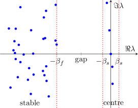
Figure 8: schematic picture of the complex plane of eigenvalues $\lambda_{m}$ (blue dots) forming two separate sets characterised by bounding parameters $\beta_{s}$ and $\beta_{f}$ of the ‘slow’ centre modes and fast stable modes, respectively.

As indicated in fig. 8 (and also fig. 9) we suppose that there are no eigenvalues with significantly positive real-part as then the linear dynamics would predict cell mode(s) with rapid exponential growth. Such ‘exploding’ modes ruin the useful of the equilibrium as a base from which to form a model. Hence we restrict attention to equilibria $\mathbb{E}$ whose spectrum has no eigenvalues with significantly positive real-part.

A rational multi-continuum model is formed by identifying a significant gap in the spectrum of cell-eigenvalues, such as that shown in fig. 8, that holds for all ${\text{\boldmath$X$}}\in{\mathbb{X}}$. In a physical application one aims to resolve macroscale time variations longer than some minimum timescale of interest $t_{s}$: in such a case one seeks a spectral gap with bounds $\beta_{s}<1/t_{s}<\beta_{f}$ (preferably $\beta_{s}\ll 1/t_{s}\ll\beta_{f}$). Identifying such a gap identifies $M$ centre cell-eigenvalues, as in fig. 8, and for convenience suppose we have indexed the eigenvalues so that these are $\lambda_{0},\ldots,\lambda_{M-1}$. Commonly there is one or two conserved cell modes (cell-eigenvalues zero) and all other eigenvalues have negative real-part, whence we may choose to identify $\beta_{s}=0$, and the argument here then leads to the common homogenised models. But if appropriate for the physical scenarios of interest, then one may alternatively choose to include more sub-cell modes in the modelling as we allow here. The corresponding $M$ cell-eigenfunctions $v_{0},\ldots,v_{M-1}$ are $M$-microscale modes that form the basis of an $M$-D subspace ${\mathbb{M}}_{\text{\boldmath$X$}}$ of ${\mathbb{H}}_{\Theta\times{\mathbb{Z}}}$ that is invariant to the linearised cell-dynamics eq. 5.6. All the other cell-modes $v_{m}$, for $m\geq M$, called stable modes, decay faster than $\operatorname{e}^{-\beta_{f}t}$. Hence, within the linearised dynamics the invariant subspace ${\mathbb{M}}_{\text{\boldmath$X$}}$ of the centre modes is exponentially quickly emergent on the chosen macroscale times $t_{s}$ of interest. Since the eigenvalue bounds hold for all ${\text{\boldmath$X$}}\in{\mathbb{X}}$, the union ${\mathbb{M}}:=\cup_{{\text{\boldmath$X$}}\in{\mathbb{X}}}{\mathbb{M}}_{\text{\boldmath$X$}}$ is an emergent global centre subspace for the collection of cell-problems over the physical domain $\mathbb{X}$. Hence $\mathbb{M}$ forms a centre subspace for the embedding pde system eq. 5.4 on $\mathbb{X}$.

In linear problems with homogeneous macroscale the ‘significant’ spectral gap may be small (e.g., section 6): one may choose a sharp distinction between the so-called centre and stable modes. The reason is that in linear, macroscale-homogeneous, problems the macroscale modes do not interact and hence do not ‘fillin’ the gap. But in problems with either nonlinear or macroscale-inhomogeneous effects (e.g., section 4.5), that we encompass here, the macroscale modes and/or variations interact to generate effects ‘within’ the gap. At high enough order these effects ‘cross’ the gap and cause troublesome small divisors, divisors that limit the order of approximation and the validity of the modelling. To avoid such small divisors one needs a gap big enough for the desired order of approximation.

The nonlinear theory of invariant manifolds for non-autonomous systems , subject to various caveats, asserts that under perturbation by nonlinearity and macroscale spatial modulation ($\text{\boldmath$\nabla$}_{\!\!{\text{\boldmath$\cal\mathchoice{\scriptstyle X}{\scriptstyle X}{\scriptscriptstyle X}{\scriptscriptstyle X}$}}}\neq 0$) the qualitative nature of this linear picture is preserved throughout $\mathbb{X}$ and $\mathbb{E}$. The theoretical support is summarised in the following sections 5.2.2 and 5.2.2.

Proposition 8 (Forward Theory).

Under sections 5 and 5.2.1, and cell-eigenvalues as in fig. 8, and when the cell-operator $\mathfrak{L}$ generates a strongly continuous semigroup, then theorems apply, such as those of Haragus & Iooss (2011) [Ch. 2], Aulbach & Wanner (2000), and Potzsche & Rasmussen (2006), to underpin the application of the spatially slowly varying analysis and results of Roberts (2015a), Bunder & Roberts (2021) to autonomous cases of the embedding system (5.4). Further, if $\mathfrak{L}$ is also bounded, then the extant theorems apply to non-autonomous cases of (5.4). Briefly, the results for the nonlinear embedding system (5.4) are the following.

1. There exists an $M$-mode centre manifold $\mathcal{M}$ in some neighbourhood of the equilibria $\mathbb{E}$.

2. All solutions in the neighbourhood of $\mathbb{E}$ are exponentially quickly attracted to solutions on $\mathcal{M}$ (approximately like $\operatorname{e}^{-\beta_{f}t}$).

3. If an approximation to $\mathcal{M}$ and the evolution thereon (the homogenisation (5.2)) satisfies (5.4) to a residual of order $N+1$ in spatial gradients, nonlinearity, and $\gamma$, and provided $N$ is constrained by the smoothness of ${\mathcal{L}},{\text{\boldmath$f$}},g$ and for nonlinear systems by the spectral gap $N+1<\beta_{f}/\beta_{s}$, then the approximations have errors of the same order $N+1$.

The three examples of sections 3, 4 and 6 all have self-adjoint linear operators for $\mathfrak{L}$ that generate the required strongly continuous semigroup. Since they are also autonomous, the above properties hold for the constructed approximations to their $M$-mode, $M$-continuum, homogenisations. Further, the example of section 6 is coded on a microscale lattice, has its cell-problem in a finite dimensional space, so $\mathfrak{L}$ is bounded, and consequently the above cited extant theory would also rigorously apply to time-dependent variations in the system. However, there are also many physical systems that do not satisfy the required preconditions for section 5.2.2 but do satisfy the less stringent preconditions of the following backward proposition.

Proposition 9 (alternate Backward Theory).

Under sections 5 and 5.2.1, and cell-eigenvalues as in fig. 8, and when ${\mathbb{H}}^{N}_{\mathbb{D}}$ is a graded Frechet space and $\mathfrak{L}$ is a continuous linear operator on ${\mathbb{H}}^{N}_{\mathbb{D}}$ in the sense of Hochs & Roberts (2019), then the theory therein underpins the application of the spatially slowly varying analysis and results of Roberts (2015a), Bunder & Roberts (2021) to the embedding system (5.4). Briefly, the results are the following:

1. there exists a constructable smooth system close to the embedding system (5.4), close to within errors of order $N+1$, an order constrained as in section 5.2.2;

2. which in a finite domain of state space containing $\mathbb{E}$ exactly possesses the constructed $M$-mode centre manifold homogenisation (5.2); and

3. where the centre manifold homogenisation is exponentially quickly emergent (approximately like $\operatorname{e}^{-\beta_{f}t}$).

In these two propositions, the statements of order $N+1$ errors and residuals justify the iterative construction algorithm described in the examples of sections 3, 4 and 6 and as implemented in the computer algebra code of appendices A, B and C.

In their review, Fish et al. (2021) [p.774] commented that in “providing a link between fine and coarse scales … the undertaking becomes challenging for heterogeneous systems, particularly for describing large deformation and failure of materials, which often involve history-dependent mechanisms.” Here we establish a framework and systematic construction whose proven supporting theory, such as these two propositions, encompasses nonlinear out-of-equilibrium modelling. Moreover, the approach often avoids the need for history-dependent mechanisms through a systematic approach to the extra kinematic variables of a multi-continuum micromorphic model.

5.2.3 Wave-like systems

Typical wave-like systems, like the elasticity homogenisation of section 6, have modal eigenvalues which are nearly pure-imaginary as illustrated schematically in fig. 9.

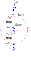
Figure 9: schematic complex plane of cell-eigenvalues $\mu+\operatorname{i}\omega$ (blue discs) in the case of wave-like dynamics when within each cell there are slow modes among fast oscillations. For small real-part $\mu$: either $\lambda_{m}=\mu_{m}+\operatorname{i}\omega_{m}$ when $\alpha=1$; or alternatively $\pm\sqrt{\lambda_{m}}=\mu_{m}+\operatorname{i}\omega_{m}$ when $\alpha=2$. The cell-eigenvalues form two separate sets characterised by bounding parameters $\beta_{s}$ and $\beta_{f}$ of the slow and fast modes, respectively.

Two usual scenarios occur: firstly, first-order systems ($\alpha=1$) are dominantly wave-like when the cell-eigenvalues are themselves all nearly pure-imaginary; and secondly, fig. 9 typically arises in the case of second-order wave systems ($\alpha=2$). In the second-order case, the eigenvalues $\lambda_{m}$ of the cell-problem eq. 5.7 give rise to two linearly independent solutions of the modal ode eq. 5.8b, namely $a_{m}(t)=A_{m}\operatorname{e}^{(\mu_{m}+\operatorname{i}\omega_{m})t}+B_{m}\operatorname{e}^{-(\mu_{m}+\operatorname{i}\omega_{m})t}$ for $\mu_{m}+\operatorname{i}\omega_{m}:=\sqrt{\lambda_{m}}$. Commonly, for $\alpha=2$, the cell-eigenvalues $\lambda_{m}$ are all (nearly) real and negative and then dynamics corresponding to fig. 9 arises for the mode solutions of (5.8b).

In these scenarios, the usual physical argument is that it is the relatively few cell-eigenvalues with small frequency $\omega_{m}$ that determine the long-time macroscale evolution. If so, then a rational multi-continuum model is formed by identifying a significant gap in the frequencies, such as that shown in fig. 9. Physically, one would usually be aiming to resolve macroscale time variations longer than some minimum timescale of interest $t_{s}$, and so seek a gap with bounds $\beta_{s}<1/t_{s}<\beta_{f}$. Identifying such a frequency gap identifies $M$ slow cell-eigenvalues, as in fig. 9, and for convenience suppose these eigenvalues correspond to $\lambda_{0},\ldots,\lambda_{M-1}$. But if appropriate for the physical application, then one may choose to include more sub-cell modes into the modelling as we allow here. The corresponding $M$ cell-eigenfunctions $v_{0},\ldots,v_{M-1}$ are $M$-microscale modes that form the basis of an $M$-D subspace ${\mathbb{M}}_{\text{\boldmath$X$}}$ of ${\mathbb{H}}_{\Theta\times{\mathbb{Z}}}$. The subspace ${\mathbb{M}}_{\text{\boldmath$X$}}$ is invariant for the linearisation of the cell-dynamics (5.6). Because the other cell-modes $v_{M},v_{M+1},\ldots$, all oscillate faster than $\operatorname{e}^{\pm\operatorname{i}\beta_{f}t}$, within the linearised dynamics the invariant subspace ${\mathbb{M}}_{\text{\boldmath$X$}}$, called a slow subspace, is expected to act as a guiding centre for the nearby dynamics of the cell problem (5.6). Since the eigenvalue bounds hold for all ${\text{\boldmath$X$}}\in{\mathbb{X}}$, the union ${\mathbb{M}}:=\cup_{{\text{\boldmath$X$}}\in{\mathbb{X}}}{\mathbb{M}}_{\text{\boldmath$X$}}$ is a global slow subspace for the collection of cell-problems over the physical domain $\mathbb{X}$. We expect $\mathbb{M}$ to be a guiding centre for the embedding pde system eq. 5.4 (e.g., van Kampen 1985, §11).

For linear systems eq. 5.4 the idea of a useful ‘guiding-centre’ slow subspace is usually sound (because of the simplicity of linear superposition of solutions).

However, for nonlinear systems eq. 5.4 a corresponding ‘guiding-centre’ slow invariant manifold is very delicate. Sijbrand (1985) established some criteria for the existence of some subcentre manifolds. But there is a long running controversy in geophysics about the non-existence of slow manifolds. Perhaps the most useful rigorous result is the following corresponding version of the backwards theory section 5.2.2 with some simple changes.

Proposition 10 (slow manifold).

Under sections 5 and 5.2.1, and cell-eigenvalues as in fig. 9, and when ${\mathbb{H}}^{N}_{\mathbb{D}}$ is a graded Frechet space and $\mathfrak{L}$ is a continuous linear operator on ${\mathbb{H}}^{N}_{\mathbb{D}}$ in the sense of Hochs & Roberts (2019), then the theory therein underpins the application of the spatially slowly varying analysis and results of Roberts (2015a), Bunder & Roberts (2021) to the embedding system (5.4). Briefly:

1. there exists a constructable smooth system close to the embedding system (5.4), close to within errors of order $N+1$, an order constrained as in section 5.2.2; and

2. which in a finite domain of state space containing $\mathbb{E}$ exactly possesses the constructed $M$-mode slow manifold homogenisation (5.2).

Moreover, a “guiding centre” is not the only justification for an $M$-mode, $M$-continuum model. Another justification for a slow manifold model is that it may be physically observable due to physical effects not encoded in the mathematics or computation. For example, one such physical mechanism is weak viscoelastic effects that damp out fast elastic waves. Another physical mechanism is that the fast waves may radiate out of the spatial domain $\mathbb{X}$ of interest to leave the slow subspace within $\mathbb{X}$: for example, sound may radiate energy from a vibrating beam; and in the atmosphere fast inertial waves propagate up into the upper atmosphere and break there leaving the bulk of the atmosphere in a quasi-geostrophic slow manifold.

Two further scenarios within this case may be invoked. The first scenario is when the perturbation $\gamma g$ forces the system near some ‘fast’ natural frequency of the cell problem, and when the forcing overcomes (weak) dissipation or radiation out of $\mathbb{X}$ of the corresponding ‘fast’ cell modes, then those fast modes may be needed in a macroscale model (e.g., Touze & Amabili 2006, Touzé & Vizzaccaro 2021). Two significant macroscale features are: firstly, the modulation of the fast mode; and secondly, the potential for nonlinear wave-wave resonance of the fast mode to drive mean ‘flow’ in the slow modes: an example is the large scale Stokes drift driven by relatively small scale ocean surface waves. However, existence and smoothness of such a model for nonlinear systems is highly problematic due to the likely plethora of nonlinear wave-wave (near) resonances with other cell-modes.

A second further scenario is either when the initial conditions are that of a near uniform small-wavelength wave, or when a localised physical initial condition together with wave dispersion combine to cause a near uniform small-wavelength in the spatial domain of interest. Then one wishes to focus purely on the one fast mode of the particular small wavelength mode, under the convenient but questionable assumption that other modes remain small. Here one would construct an invariant manifold describing the large-scale modulation of the wave from a linear base of the one mode, and via embedding the system in the ensemble of all phase-shifts of the wave (Roberts 2015a, §2.5). Generally, the resulting models are variants of the so-called nonlinear Schrödinger pde. The existence and smoothness of such a model is highly problematic due to potential nonlinear (near) resonances, but again backwards theory could assert there is a system close to that specified which exactly possesses the constructed invariant manifold. When the initial conditions possess multiple identifiable waves, then like the quasi-periodic cases herein, embedding the system in the ensemble of all phase-shifts independently should systematically lead to a model expressed in interacting nonlinear Schrödinger pdes.

5.2.4 Fractional differential evolution

In this case let the time differential operator $\partial_{t}^{\alpha}$ for real fractional $\alpha\in(0,2)\mathchar 8507\relax{}\alpha\neq 1$, be interpreted in the Caputo sense and implicitly from initial time $t=0$. Let’s reconsider the general solution eq. 5.8 for the linearised cell-problem eq. 5.6. From the general solution (5.9) derived in appendix D, the general solution to the $m$th-mode fractional differential equation (fde) eq. 5.8b, $\partial_{t}^{\alpha}a_{m}=\lambda_{m}a_{m}$ , is, in terms of parameter $\mu_{m}:=(-\lambda_{m})^{1/\alpha}$,

$$a_{m}(t)=C_{m0}\operatorname{e}_{\alpha}^{(0)}(\mu_{m}t)+\begin{cases}0,&0<\alpha<1\,,\\ C_{m1}\operatorname{e}_{\alpha}^{(-1)}(\mu_{m}t),&1<\alpha<2\,.\end{cases}$$ (5.9)

The free constants $C_{m0},C_{m1}$ happen to be proportional to the derivatives at time zero: $C_{mk}\propto a_{m}^{(k)}(0^{+})$. The functions $\operatorname{e}_{\alpha}^{(0)}(t):=E_{\alpha,1}(-t^{\alpha})$ and $\operatorname{e}_{\alpha}^{(-1)}(t):=tE_{\alpha,2}(-t^{\alpha})$ (appendix D) in terms of the Mittag–Leffler function $E_{\alpha,\beta}(z):=\sum_{k=0}^{\infty}\frac{z^{k}}{\Gamma(\alpha k+\beta)}$ (e.g., Gorenflo & Mainardi 1997, (A.1)).

Arguably, the most important aspect of the general solution (5.9) is its behaviour for large time in the most common case of real negative eigenvalues $\lambda_{m}$. In this case $\mu_{m}=(-\lambda_{m})^{1/\alpha}$ is real and positive and we need only consider the general solution for real positive arguments to $\operatorname{e}_{\alpha}^{(k)}$. Since $E_{\alpha,\beta}(z)\sim(-z)^{-1}/\Gamma(\beta-\alpha)$ as $|z|\to\infty$ with $|\arg(-z)|<\pi(1-\alpha/2)$, appendix D derives that $\operatorname{e}_{\alpha}^{(k)}$ generically decay algebraically to zero:

$$\operatorname{e}_{\alpha}^{(0)}(t)\sim\frac{t^{-\alpha}}{\Gamma(1-\alpha)}\,, \operatorname{e}_{\alpha}^{(-1)}(t)\sim\frac{t^{1-\alpha}}{\Gamma(2-\alpha)}\,, \text{as }t\to+\infty\,.$$ (5.10)

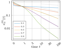
Figure 10: For the fde (5.8b), plot the general solution (5.9) component $\operatorname{e}_{\alpha}^{(0)}(t)$ for five $\alpha\in(0,1)$ (as in legend). The time axis is quasi-log via an asinh scaling of the axis, and so clearly shows the long-time algebraic decay of this component in the general solution. The dotted lines are the large time asymptotics (5.10).

fig. 10 plots the numerically computed solution component $\operatorname{e}_{\alpha}^{(0)}(t)$ for various $0<\alpha<1$ with the large-time approximations (5.10). The log-log nature of the plot clearly exhibits the long-time algebraic decay of this component of the general solution eq. 5.9, with the decay and the approach to the asymptotes very slow for small $\alpha$. For the larger case of $\alpha=0.9$, $\operatorname{e}_{\alpha}^{(0)}(t)$ exhibits exponential-like decay for small time, $t<5$—characteristic of the exponential decay for the ode case of $\alpha=1$—before morphing to algebraic decay for larger times, $t>10$ .

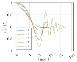
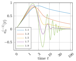
Figure 11: For the fde (5.8b), plots the two general solution (5.9) components for five $\alpha\in(1,2)$ (see legend): (left) $\operatorname{e}_{\alpha}^{(0)}(t)$; (right) $\operatorname{e}_{\alpha}^{(-1)}(t)$. The time axis is quasi-log via an asinh scaling of the axis.

For the higher range $1<\alpha<2$ , fig. 11 plots the two solution components $\operatorname{e}_{\alpha}^{(0)}(t)$ and $\operatorname{e}_{\alpha}^{(-1)}(t)$ . These components oscillate some number of times—the number of oscillations increase as $\alpha\to 2$ (the wave case)—before eventually morphing into the large time algebraic decay of the asymptotic (5.10).

Now let’s address what the above means for modelling and/or homogenisation of general systems (5.1). The clearest case is for linear autonomous systems (5.1) and when the cell eigen-problem (5.7) has a robust spectrum, such as obtained from a self-adjoint cell-operator $\mathfrak{L}$. Then the modal fdes (5.8b) are robust under perturbations by macroscale spatial gradients. Consequently, under such perturbations we expect each mode to still evolve roughly like $(-\lambda_{m}t)^{-\alpha-1+\hat{\alpha}}$ for large time, where $\hat{\alpha}:=\lceil\alpha\rceil={}$nearest integer${}\geq\alpha$, and provided $|\arg(-\lambda_{m})|\leq\vartheta_{\max}<\pi(1-\alpha/2)$ for some angle bound $\vartheta_{\max}$. Because of the eigenvalue factor $\lambda_{m}$, the modes with large $|\lambda_{m}|$ decay the quickest, albeit with the same exponent. The result is that we reasonably expect that the large time evolution is dominated by the modes with small $|\lambda_{m}|$. Then, as in the exponential case of section 5.2.2, we may reasonably construct and use a multi-modal, multi-continuum, homogenisation based upon choosing the $M$-modes with smallest $|\lambda_{m}|$.

The above argument reasonably justifies homogenisations such as (LABEL:Epde2,EEhcegManifold2,EEhcegManifold3) for general fractional $\alpha$.

However, nonlinearities and non-autonomous forcing complicates the situation. There is some extant theory of invariant manifolds for fractional differential systems (e.g., Cong et al. 2016, Ma & Li 2015), but none appears suitable to invoke for general systems (5.1). I conjecture that adapting proposed backwards theory Roberts (2022), Hochs & Roberts (2019) would provide the most accessible route for supporting invariant manifold homogenisation of nonlinear non-autonomous fde systems. However, it remains to be established whether or not a given fde system is generally ‘close’ to a diffeomorphism of a constructible fde system which is in the separated canonical form.

5.2.5 Improving spatial resolution

sections 5.2.2, 5.2.3 and 5.2.4 focussed upon the scenario when one choose multi-modal multi-continua homogenisations based upon selecting those modes with the longest lifetime. But there is significant interest in scenarios where the prime motivation is to better resolve spatial structures. For two examples: Alavi et al. (2023) [p.2164] comment that “Enriched continuum theories are required in such situations to capture the effect of spatially rapid fluctuations at the mesoscopic and macroscopic levels”; and Somnic & Jo (2022) [p.8] wrote “Classical continuum theory is not suitable when … high strain gradients are observed in the domain”. Hence this section discusses possibilities for choosing invariant manifold modes based upon the criterion of improving the spatial resolution irrespective of the time resolution.

Often the two criteria, spatial resolution and time resolution, are essentially equivalent. In that common case the previous discussions apply. This equivalence is generally the case for nonlinear systems because nonlinearity typically has mode interactions which spread the dynamical energy among all modes, and so all modes are generally excited. It is only in the special circumstance when the nonlinear system and the initial conditions preserve some symmetry that space and time resolutions are not necessarily equivalent, For example, in the nonlinear Burgers’ pde $u_{t}=-uu_{x}+u_{xx}$ odd functions are preserved, so that if the initial conditions are odd, then cosine modes need not be included in a model, only sines.

However, in linear systems (most of sections 3, 4 and 6) symmetries are more likely to be preserved. For example, in the multi-modal multi-continua modelling of shear dispersion along a channel Watt & Roberts (1995) found even modes across the channel interacted with the leading mean mode, but the odd modes did not. Consequently the two-mode bi-continua model based upon the leading two even modes has much improved spatial resolution , when compared to that of the leading order model, but no improvement of the temporal resolution because the two-even-mode model neglects the gravest odd-mode (which has the slowest decay rate). Quantitive estimates of the spatial resolution may be made for linear systems, section 3.2.2 for example, by constructing to 20th order or more in $\partial_{x}$, taking the Fourier transform which converts macroscale spatial derivatives to multiplication by the macroscale wavenumber $k$, that is, $\partial_{x}\equiv\operatorname{i}k$ . Then a Domb–Sykes plot (Domb & Sykes 1957, Hunter 1987, e.g.) or Mercer–Roberts plot (Mercer & Roberts 1990, Appendix) for series’ in the wavenumber $k$ predict the convergence limiting singularity in the complex $k$-plane, and hence the radius of convergence, say $k_{*}$. The minimum resolved wavelength by the model is then deduced to be $2\pi/k_{*}$.

One way to view an invariant manifold for linear systems is as a perturbation from the cell-problem (5.6) in small macroscale wavenumber $k$. A crucial characteristic of the modelling are the eigenvalues $\lambda(k)$ as a perturbative function of the wavenumber $k$. Let’s explore fascinating aspects of such a multi-mode, multi-continuum, homogenisation via the mathematical structure of perturbative eigenvalue problems (e.g., Bender & Orszag 1981, §7.5).

The crucial property of eigenproblems for a given $n\times n$ matrix that is a function of a parameter $k$ is that its eigenvalue function $\lambda(k)$ generally forms a single $n$-sheeted (Riemann) surface in complex $k$ (e.g., Bender & Orszag 1981, p.350). Such an $n$-sheeted surface possesses various branch points at complex $k$ that are necessary to connect the sheets together into a unified whole. Although, in some cases, often due to symmetries, the $n$-sheeted surface partitions into several disjoint sheeted surfaces. These properties also generalises to many pde operators of interest in applications.

The branch points in the Riemann sheets are singularities that limit the convergence of the perturbative expansion for $\lambda(k)$ in wavenumber $k$, and hence limit the spatial resolution of the macroscale homogenisation. For example, the tri-continuum high-order homogenisation of section 3.2.2 shows the eigenvalue sheet of the homogenisation, for small heterogeneity $a$, has pole singularities at real wavenumbers $k=\pm 3/2$, pole singularities that limit the resolution of the homogenisation in physical space. But the question is: which branch-points become limiting?

Using the developed rigorous framework and systematic procedure we may construct multi-modal multi-continua homogenisations to any chosen order. For linear systems, such an $M$-mode, $M$-continua homogenisation constructs a homogenisation whose eigenvalues $\lambda$ form an $M$-sheeted Riemann surface as an analytic function, say $\lambda^{M}(k)$, of wavenumber $k$ in the complex $k$-plane. The original system also has a many-sheeted analytic eigenvalue function $\lambda(k)$. The $M$-mode homogenisation approximates $\lambda(k)$ by analysing effects and interactions of the $M$ chosen modes of the cell-problem—modes chosen from the eigenvalue spectrum at zero wavenumber (section 5.2.1). The systematic construction guarantees that the perturbation series of $\lambda^{M}(k)$ is identical with that of the $M$ chosen Riemann sheets of the original $\lambda(k)$. Consequently, we expect an $M$-mode homogenisation to encompass smoothly all branch-point singularities in the original $\lambda(k)$ that arise through interactions among the chosen $M$-modes (whether physical singularities at real $k$, or unphysical at complex valued $k$). Branch-point singularities in $\lambda(k)$ that occur, physically or not, due to interactions between the $M$-chosen modes and all the other unchosen modes cannot be captured in the $M$-mode homogenisation, and so it is these singularities that generally limit the radius of convergence of the $M$-continuum homogenisation. It is this limit in wavenumber $k$ that then translates to a limit on the spatial macroscales accurately resolvable in a chosen $M$-mode, $M$-continuum homogenisation.

Consequently, to obtain the best macroscale spatial resolution in a multi-mode multi-continua homogenisation, without considering temporal resolution, one needs to select the $M$-modes that interact and form the nearest branch-points of the eigenvalue $\lambda(k)$ Riemann surface. However, such selection is usually difficult because commonly the near branch-point singularities are at unphysical complex-valued wavenumbers for no known physical reason. Unless there are known physical symmetries, the best practical general guide to improve macroscale spatial resolution appears to be to select those modes with the longest time scale, as discussed in sections 5.2.2, 5.2.3 and 5.2.4.

5.3 Construct a chosen invariant manifold multi-continuum homogenisation

The construction of multi-continuum homogenisation in multiple large spatial dimensions relies on theory proven by Bunder & Roberts (2021), which in turn rests on general theory by Aulbach & Wanner (2000), Potzsche & Rasmussen (2006), Hochs & Roberts (2019). One of the crucial theoretical results is that if a derived approximation satisfies the embedding pde eq. 5.4 to a residual of $\mathcal{O}\mathchoice{\big{(}\partial_{\text{\boldmath$\cal\mathchoice{\scriptstyle X}{\scriptstyle X}{\scriptscriptstyle X}{\scriptscriptstyle X}$}}^{N+1}\big{)}}{\big{(}\partial_{\text{\boldmath$\cal\mathchoice{\scriptstyle X}{\scriptstyle X}{\scriptscriptstyle X}{\scriptscriptstyle X}$}}^{N+1}\big{)}}{(\partial_{\text{\boldmath$\cal\mathchoice{\scriptstyle X}{\scriptstyle X}{\scriptscriptstyle X}{\scriptscriptstyle X}$}}^{N+1})}{(\partial_{\text{\boldmath$\cal\mathchoice{\scriptstyle X}{\scriptstyle X}{\scriptscriptstyle X}{\scriptscriptstyle X}$}}^{N+1})}$, then the corresponding homogenisation is correct to an error $\mathcal{O}\mathchoice{\big{(}\partial_{\text{\boldmath$\cal\mathchoice{\scriptstyle X}{\scriptstyle X}{\scriptscriptstyle X}{\scriptscriptstyle X}$}}^{N+1}\big{)}}{\big{(}\partial_{\text{\boldmath$\cal\mathchoice{\scriptstyle X}{\scriptstyle X}{\scriptscriptstyle X}{\scriptscriptstyle X}$}}^{N+1}\big{)}}{(\partial_{\text{\boldmath$\cal\mathchoice{\scriptstyle X}{\scriptstyle X}{\scriptscriptstyle X}{\scriptscriptstyle X}$}}^{N+1})}{(\partial_{\text{\boldmath$\cal\mathchoice{\scriptstyle X}{\scriptstyle X}{\scriptscriptstyle X}{\scriptscriptstyle X}$}}^{N+1})}$ (Bunder & Roberts 2021, §3). This direct connection between residual and error follows on from earlier theory by Potzsche & Rasmussen (2006) on approximating inertial manifolds. In multi-D space, practical procedures to derive approximations to any chosen order of residual are in this section generalised from those of section 2.2.3 for 1-D space and from earlier developments (Roberts 2015b, Part III).

For linear problems, the following may apply for a wide variety of time evolution operators $\partial_{t}^{\alpha}$. However, to encompass nonlinear problems this section addresses the case of first-order time derivatives, $\alpha=1$. For nonlinear systems with second-order time derivatives ($\alpha=2$), introduce ‘velocity’ variables to rewrite the system as a larger system of first-order.

The general procedure is especially suitable for computer algebra (appendix C) as applied for example to the homogenisation of 2-D heterogeneous elasticity (section 6). For $M$ selected modes (section 5.2), define the vector of local amplitudes ${\text{\boldmath$U$}}(t,{\text{\boldmath$\cal\mathchoice{\scriptstyle X}{\scriptstyle X}{\scriptscriptstyle X}{\scriptscriptstyle X}$}}):=(U_{0},\ldots,U_{M-1})$. We seek an invariant manifold of the embedding pde eq. 5.4 in the form ${\mathfrak{u}}=v({\text{\boldmath$U$}},t,{\text{\boldmath$\cal\mathchoice{\scriptstyle X}{\scriptstyle X}{\scriptscriptstyle X}{\scriptscriptstyle X}$}},{\text{\boldmath$\theta$}})$ such that $\partial_{t}^{\alpha}{\text{\boldmath$U$}}=G({\text{\boldmath$U$}},t,{\text{\boldmath$\cal\mathchoice{\scriptstyle X}{\scriptstyle X}{\scriptscriptstyle X}{\scriptscriptstyle X}$}})$ where the right-hand side dependence upon $U$ implicitly involves its general gradients ${\text{\boldmath$U$}}_{{{\cal\mathchoice{\scriptstyle X}{\scriptstyle X}{\scriptscriptstyle X}{\scriptscriptstyle X}}}_{i}}\mathchar 8507\relax{}{\text{\boldmath$U$}}_{{{\cal\mathchoice{\scriptstyle X}{\scriptstyle X}{\scriptscriptstyle X}{\scriptscriptstyle X}}}_{i}{{\cal\mathchoice{\scriptstyle X}{\scriptstyle X}{\scriptscriptstyle X}{\scriptscriptstyle X}}}_{j}}\mathchar 8507\relax{}\ldots$, and the explicit $(t,{\text{\boldmath$\cal\mathchoice{\scriptstyle X}{\scriptstyle X}{\scriptscriptstyle X}{\scriptscriptstyle X}$}})$ dependence are the slow, macroscale, variations arising from macroscale functional graduations in the problem. For any given approximations $\tilde{v},\tilde{G}$ to $v,G$, compute the residual of the embedding pde eq. 5.4, call it $\operatorname{Res}(\tilde{v},\tilde{G})$. Compute corrections $v^{\prime},G^{\prime}$ to the approximations $\tilde{v},\tilde{G}$ by solving a variant of the cell problem (5.6), linearised and forced by the residual, called the homological equation,

$${\mathfrak{L}}v^{\prime}-\sum_{m=0}^{M-1}\mathchoice{\frac{\partial v^{\prime}}{\partial U_{m}}}{{\partial v^{\prime}}/{\partial U_{m}}}{{\partial v^{\prime}}/{\partial U_{m}}}{{\partial v^{\prime}}/{\partial U_{m}}}(\lambda_{m}U_{m}+\zeta_{m}U_{m+1})-\sum_{m=0}^{M-1}v_{m}G^{\prime}_{m}=\operatorname{Res}(\tilde{v},\tilde{G}).$$ (5.11)

As in section 2.2.3, the factors $(\mathchoice{\frac{\partial v^{\prime}}{\partial U_{m}}}{{\partial v^{\prime}}/{\partial U_{m}}}{{\partial v^{\prime}}/{\partial U_{m}}}{{\partial v^{\prime}}/{\partial U_{m}}})U_{n}$ have to be interpreted in the Calculus of Variations sense such that here it represents $v^{\prime}_{U_{m}}U_{n}+\sum_{i}v^{\prime}_{U_{m{{\cal\mathchoice{\scriptstyle X}{\scriptstyle X}{\scriptscriptstyle X}{\scriptscriptstyle X}}}_{i}}}U_{n{{\cal\mathchoice{\scriptstyle X}{\scriptstyle X}{\scriptscriptstyle X}{\scriptscriptstyle X}}}_{i}}+\sum_{i,j}v^{\prime}_{U_{m{{\cal\mathchoice{\scriptstyle X}{\scriptstyle X}{\scriptscriptstyle X}{\scriptscriptstyle X}}}_{i}{{\cal\mathchoice{\scriptstyle X}{\scriptstyle X}{\scriptscriptstyle X}{\scriptscriptstyle X}}}_{j}}}U_{n{{\cal\mathchoice{\scriptstyle X}{\scriptstyle X}{\scriptscriptstyle X}{\scriptscriptstyle X}}}_{i}{{\cal\mathchoice{\scriptstyle X}{\scriptstyle X}{\scriptscriptstyle X}{\scriptscriptstyle X}}}_{j}}+\cdots$ where these subscript-derivatives of $v^{\prime}$ are done with respect to the subscript symbol Roberts (1988). Recall that $\zeta_{m}$ arises with generalised eigenmodes (section 5.2.1). Differences in (5.11) from the usually used cell-problems arise in this systematic invariant manifold framework through accounting for the physical out-of-equilibrium effects. After solving (5.11) for $v^{\prime},G^{\prime}$, then update the approximations $\tilde{v},\tilde{G}$, and iterate until the residual is of the order of the desired error.

Two practical simplifications are often feasible for solving the homological equation (5.11). Firstly, neglect the term in $\zeta_{m}$ arising from generalised eigenmodes. This neglect increases the number of required iterations by no more than a factor equal to the multiplicity of the eigenvalues. Secondly, when constructing nonlinear models to errors of order $p$ in nonlinearity, provided the spectral gap $(\beta_{s},\beta_{f})$ (see figs. 8 and 9) is big enough so that the ratio $\beta_{f}/\beta_{s}>p$ then one can neglect the term in $\lambda_{m}$ as well. Thus, in practice one often determines updates by solving the simpler common homological equation

$${\mathfrak{L}}v^{\prime}-\sum_{m=0}^{M-1}v_{m}G^{\prime}_{m}=\operatorname{Res}(\tilde{v},\tilde{G}).$$ (5.12)

The iterative updates are then not exact (unless $\beta_{s}=0$), but the residual generally improves each iteration. One terminates the iteration when the coefficients in the residual are all smaller than some small numerical threshold such as $10^{-7}$. The elasticity homogenisation code of appendix C generally invokes both of these simplifications, and so solves (5.12) for updates.

6 Example in 2D elasticity homogenisation

This section applies the approach of section 5 to rigorously construct and support a second-order in time, tri-continuum, three-mode, homogenisation of 2D elasticity for an example heterogeneous Young’s modulus.

We adopt simple robust microscale equations for the heterogeneous 2-D elasticity. On the staggered microscale $xy$-grid of fig. 12, of spacing $\delta x$ and $\delta y$, define the displacements: $\color[rgb]{0,0,1}\blacktriangleright$, horizontal $u_{ij}(t)$; $\color[rgb]{1,0,0}\blacktriangle$, vertical $v_{ij}(t)$.

Figure 12: a small part of the microscale grid, of spacing $\delta x$ and $\delta y$, used to code 2-D elasticity. The grid is staggered on the microscale: $\color[rgb]{0,0,1}\blacktriangleright$, horizontal displacements and velocities; $\color[rgb]{1,0,0}\blacktriangle$, vertical displacements and velocities; $\color[rgb]{0,0.7,0}\circledcirc$, $\color[rgb]{0,0.7,0}\otimes$, components of strain and stress tensor (6.1).

The adopted microgrid elasticity uses centred finite differences, $\delta_{i}$ and $\delta_{j}$, to compute stresses at the shown microscale grid-points (fig. 12):

$$\text{$\color[rgb]{0,0.7,0}\otimes$}\quad\sigma_{ij}^{xy}:=\mu_{ij}\big{[}\delta_{i}v_{ij}/\delta x+\delta_{j}u_{ij}/\delta y\big{]};$$ (6.1a)

$$\text{$\color[rgb]{0,0.7,0}\circledcirc$}\quad\sigma_{ij}^{xx}:=(\lambda_{ij}+2\mu_{ij}){\delta_{i}u_{ij}}/{\delta x}+\lambda_{ij}{\delta_{j}v_{ij}}/{\delta y}\,;$$ (6.1b)

$$\text{$\color[rgb]{0,0.7,0}\circledcirc$}\quad\sigma_{ij}^{yy}:=\lambda_{ij}{\delta_{i}u_{ij}}/{\delta x}+(\lambda_{ij}+2\mu_{ij}){\delta_{j}v_{ij}}/{\delta y}\,,$$ (6.1c)

where $\lambda_{ij},\mu_{ij}$ denote the heterogeneous Lamé parameters. Then centred finite differences compute the following (non-dimensional) acceleration odes

$$\text{$\color[rgb]{0,0,1}\blacktriangleright$}\quad\partial_{t}^{2}u_{ij}={\delta_{i}\sigma_{ij}^{xx}}/{\delta x}+{\delta_{j}\sigma_{ij}^{xy}}/{\delta y}\,,$$ (6.2a)

$$\text{$\color[rgb]{1,0,0}\blacktriangle$}\quad\partial_{t}^{2}v_{ij}={\delta_{i}\sigma_{ij}^{xy}}/{\delta x}+{\delta_{j}\sigma_{ij}^{yy}}/{\delta y}\,.$$ (6.2b)

The Lamé parameters which appear in the stresses (6.1) are defined as

$$\lambda_{ij}:=\frac{\nu_{ij}E_{ij}}{(1+\nu_{ij})(1-2\nu_{ij})},\quad\mu_{ij}:=\frac{E_{ij}}{2(1+\nu_{ij})},$$ (6.3)

in terms of Young’s modulus $E_{ij}$ and Poisson ratio $\nu_{ij}$.

6.1 Example cell problem

Suppose the microscale heterogeneity is reflected in the Lamé parameters $\lambda_{ij}$ and $\mu_{ij}$ being $n_{x}$-periodic in $i$ and $n_{y}$-periodic in $j$. That is, the material is $\ell_{x}:=n_{x}\delta x$ periodic in the $x$-direction and $\ell_{y}:=n_{y}\delta y$ periodic in the $y$-direction.

We choose to non-dimensionlise on the microscale cell size, choosing the length scale so that each cell is $1$-periodic in $x,y$.

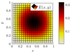
Figure 13: example of one period, one cell, of the 2-D microscale heterogeneity in the Young’s modulus $E=\big{[}0.01+|\sin(\pi x)\sin(\pi y)|\big{]}/\pi$. The non-dimensionalised microscale periods are $\ell_{x}=\ell_{y}=1$.

fig. 13 plots one such non-dimensional microscale cell of the example Young’s modulus used herein for the case reported here with $n_{x}=n_{y}=10$. The material is made up of these cells repeating indefinitely in the $xy$-plane. This microscale heterogeneity is similar to the §§3–5 example of Sarhil et al. (2024) (diagrams phase-shifted in each cell). The homogenisation model then describes the evolution of elastic waves which have wavelengths significantly larger than one; that is, in this non-dimensionalisation the macroscale wavenumbers are those significantly less than $2\pi$.

The general basic cell-problem eq. 5.6 is here to solve the heterogeneous system eqs. 6.1 and 6.2 on a cell with periodic boundary conditions as justified by section 6.2. But we obtain a preliminary physical understanding of general cell solutions by exploring the eigenvalues and eigenvectors of the cell eigenproblem (5.7) corresponding to the physical eqs. 6.1 and 6.2.

For the particular example of fig. 13, with microgrid $n_{x}=n_{y}=10$ in each cell, appendix C computes the $128\times 128$ Jacobian matrix $J$ of the right-hand side of the elasticity equations eq. 6.2, and then computes its eigenvalues and eigenvectors. The smallest five eigenvalues are $\lambda_{0}=\lambda_{1}=0\mathchar 8507\relax{}\lambda_{2}=-0.6431\mathchar 8507\relax{}\lambda_{3}=-1.2653\mathchar 8507\relax{}\lambda_{4}=-1.2886\mathchar 8507\relax{}\ldots$ . fig. 14 plots the displacement fields of the eigenvectors corresponding to the three smallest eigenvalues.

Figure 14: for microscale heterogeneity of fig. 13, the eigenvectors $v_{m}$ of the three slowest modes. Shown are the displacement vectors of the modes: two modes with $\lambda_{0}=\lambda_{1}=0$ are rigid body translations; the third with $\lambda_{2}\approx-0.64$ is a microscale sub-cell rotation—the slowest sub-cell mode. The next two eigenvalues are $\lambda_{3}\approx-1.27$ and $\lambda_{4}\approx-1.29$.

To form a macroscale model to be valid all times-scales longer than some threshold, in this problem with second-order derivatives in time, we must resolve all waves with corresponding period longer than the threshold, that is, with frequencies smaller than some threshold. In this non-dimensional example, the frequencies of the waves, $\omega_{m}=\sqrt{-\lambda_{m}}$ , corresponding to the computed spectral modes (fig. 14) are $\omega_{0}=\omega_{1}=0\mathchar 8507\relax{}\omega_{2}=0.8019\mathchar 8507\relax{}\omega_{3}=1.1248\mathchar 8507\relax{}\omega_{4}=1.1352\mathchar 8507\relax{}\ldots$ .

• The usual homogenisation model is based upon averaging over a cell, and these averages are usually done with a constant weight function. Such constant weights implicitly correspond to the two sub-cell uniform displacement eigenvectors of fig. 14.

  In the multi-continuum framework proposed and developed herein, we arrive at the same basis as the usual homogenisation, but by a different rationale (section 5.2.3). The rationale is to choose to resolve all dynamics with a timescale longer than some threshold, say we choose a threshold approximately $5$. Then we base our modelling on all sub-cell modes with frequencies smaller than $1/5=0.2$ (roughly). Here the two ‘rigid body’ cell-modes of fig. 14 corresponding to $\omega_{0}=\omega_{1}=0$ are the only modes with frequency $\omega_{m}<0.2$. Hence we would choose a bi-continuum two-mode model. In such a macroscale model, these two sub-cell modes are modulated over the macroscale of many cells. The homogenisation describes such macroscale modulation.

• However, observe that here the third frequency $\omega_{2}\approx 0.8$ is separated by a gap from the higher frequencies $\omega_{3},\omega_{4},\ldots\geq 1.1$ (albeit only a small gap). Hence, if we choose to want to resolve dynamics on a timescale longer than the smaller threshold of $1.0$ say, then we should choose a homogenisation based upon the three sub-cell modes of smallest frequency. The third mode, plotted in fig. 14, corresponds to rotations of the ‘hard’ core in the centre of each cell (fig. 13). In the macroscale modelling, this third mode represents the relatively slow vibration of such sub-cell rotations and how they interact and evolve over a large spatial domain.

  This three-mode tri-continuum homogenisation is the example choice that we develop here, and the result is a rigorous homogenisation for the macroscale wave dynamics.

• We could choose more ‘slowest’ modes to form a multi-continuum homogenisation with more modes characterising the dynamics of more microscale physics.

6.2 Phase-shift embedding of the 2D heterogeneity

As in previous sections, a multi-continuum homogenisation is rigorously achieved via embedding the physical system in the ensemble of all phase-shifts of the heterogeneity. The embedding of (LABEL:EEstress,EEaccel) is done by considering horizontal displacement field ${\mathfrak{u}}_{ijkl}(t)$ on a 4-D ‘spatial’ lattice in $xy\theta\phi$-space, and similarly for the other fields $\mathfrak{v},\sigma^{xx},\sigma^{xy},\sigma^{yy}$. For simplicity, let the sub-cell lattice spacings $\delta\theta=\delta x$ and $\delta\phi=\delta y$ . Then the spatial domain for the 4-D lattice is ${\mathbb{R}}^{2}\times[0,\ell_{x})\times[0,\ell_{y})$, with all fields $\ell_{x},\ell_{y}$-periodic in $\theta,\phi$ respectively. In terms of the shift operator $E_{i}$ defined so that $E_{i}^{r}{\mathfrak{u}}_{ijkl}:={\mathfrak{u}}_{i+r,jkl}$ and similarly for $j,k,l$, define the centred difference operator

$${\bar{\delta}}_{pq}:=E^{\frac{1}{2}}_{p}E^{\frac{1}{2}}_{q}-E^{-\frac{1}{2}}_{p}E^{-\frac{1}{2}}_{q}\,,\quad\text{for }p,q\in\{i,j,k,l\},$$ (6.4)

which is a centred difference along diagonals in the $ijkl$-lattice. Then consider the following system that embeds eqs. 6.1 and 6.2:

$$\text{$\color[rgb]{0,0.7,0}\otimes$}\quad\sigma_{ijkl}^{xy}:=\mu_{kl}\big{[}{\bar{\delta}}_{jl}{\mathfrak{u}}_{ijkl}/\delta y+{\bar{\delta}}_{ik}\mathfrak{v}_{ijkl}/\delta x\big{]};$$ (6.5a)

$$\text{$\color[rgb]{0,0.7,0}\circledcirc$}\quad\sigma_{ijkl}^{xx}:=(\lambda_{kl}+2\mu_{kl}){{\bar{\delta}}_{ik}{\mathfrak{u}}_{ijkl}}/{\delta x}+\lambda_{kl}{{\bar{\delta}}_{jl}\mathfrak{v}_{ijkl}}/{\delta y}\,;$$ (6.5b)

$$\text{$\color[rgb]{0,0.7,0}\circledcirc$}\quad\sigma_{ijkl}^{yy}:=\lambda_{kl}{{\bar{\delta}}_{ik}{\mathfrak{u}}_{ijkl}}/{\delta x}+(\lambda_{kl}+2\mu_{kl}){{\bar{\delta}}_{jl}\mathfrak{v}_{ijkl}}/{\delta y}\,;$$ (6.5c)

$$\text{$\color[rgb]{0,0,1}\blacktriangleright$}\quad\partial_{t}^{2}{\mathfrak{u}}_{ijkl}={{\bar{\delta}}_{ik}\sigma_{ijkl}^{xx}}/{\delta x}+{{\bar{\delta}}_{jl}\sigma_{ijkl}^{xy}}/{\delta y}\,;$$ (6.5d)

$$\text{$\color[rgb]{1,0,0}\blacktriangle$}\quad\partial_{t}^{2}\mathfrak{v}_{ijkl}={{\bar{\delta}}_{ik}\sigma_{ijkl}^{xy}}/{\delta x}+{{\bar{\delta}}_{jl}\sigma_{ijkl}^{yy}}/{\delta y}\,.$$ (6.5e)

By the form of the embedding eq. 6.5 every solution ${\mathfrak{u}}_{ijkl}(t),\mathfrak{v}_{ijkl}(t)$ to eq. 6.5 gives rise to solutions of the original physical system eqs. 6.1 and 6.2, for every phase-shift of the elasticity parameters. To see this, for every $k^{\prime},l^{\prime}$ define $u^{\prime}_{ij}:={\mathfrak{u}}_{ij,i+k^{\prime},j+l^{\prime}}$ and similarly for the other fields. Then eq. 6.5, satisfied by ${\mathfrak{u}}_{ijkl}(t),\mathfrak{v}_{ijkl}(t)$, reduces to the original eqs. 6.1 and 6.2 for $u^{\prime}_{ij}$ with Lamé parameters $\lambda_{ij},\mu_{i,j}$ replaced by their phase shifts $\lambda_{i+k^{\prime},j+l^{\prime}}\mathchar 8507\relax{}\mu_{i+k^{\prime},j+l^{\prime}}$. In particular, for $k^{\prime}=l^{\prime}=0$ this defined $u^{\prime}_{ij}$, with corresponding other fields, satisfies the original eqs. 6.1 and 6.2.

Similarly, an ensemble of all solutions to the ensemble of phase-shifted problems eqs. 6.1 and 6.2 forms a solution to the embedding eq. 6.5. That is, the embedding system eq. 6.5, homogeneous in $x,y$, is equivalent to the ensemble of phase-shifts of the given heterogeneous system eqs. 6.1 and 6.2.

6.3 Basis of invariant manifolds

The invariant manifold, multi-continuum, micromorphic, framework wraps around whatever microscale code a user supplies—here it is the embedded microscale system (6.5). The 4-D lattice system (6.5) is not a pde, nonetheless the same framework eq. 5.6 of section 5.2.1 applies. The reason is that the operators and functions in the general form eq. 5.6 may be microscale-nonlocal in space Roberts (2021). Indeed, extant forward theory of invariant manifolds is easier to apply to such spatially discrete systems as, crucially, the difference operators are bounded, whereas the usual alternative of spatial derivatives are troublesome because derivatives are unbounded operators.

In the practical construction of invariant manifold models (appendix C), the spatial differences may be written in terms of shift operators when convenient (as in (6.5)), or equivalent differential operators when that is convenient.

For macroscale modelling of homogenised dynamics, the valid scenarios are that variations in $x,y$ are slow in some useful sense. The basis of the modelling is the case where there are effectively no variations in $x,y$, hence the microscale shifts $E_{i}{\mathfrak{u}}_{ijkl}\approx{\mathfrak{u}}_{ijkl}$ and similarly for all fields, that is, $E_{i},E_{j}\mapsto 1$ . In this base case, the centred difference operators ${\bar{\delta}}_{ik}\mapsto\delta_{k}$ and ${\bar{\delta}}_{jl}\mapsto\delta_{l}$. Consequently, in this base case, at each and every cross section, parametrised by $x,y$ or equivalently indexed by $i,j$ which I omit for brevity, the embedding system (6.5) reduces to the cell-problem

$$\text{$\color[rgb]{0,0.7,0}\otimes$}\quad\sigma_{kl}^{xy}:=\mu_{kl}\big{[}\delta_{k}\mathfrak{v}_{kl}/\delta x+\delta_{l}{\mathfrak{u}}_{kl}/\delta y\big{]};$$ (6.6a)

$$\text{$\color[rgb]{0,0.7,0}\circledcirc$}\quad\sigma_{kl}^{xx}:=(\lambda_{kl}+2\mu_{kl}){\delta_{k}{\mathfrak{u}}_{kl}}/{\delta x}+\lambda_{kl}{\delta_{l}\mathfrak{v}_{kl}}/{\delta y}\,;$$ (6.6b)

$$\text{$\color[rgb]{0,0.7,0}\circledcirc$}\quad\sigma_{kl}^{yy}:=\lambda_{kl}{\delta_{k}{\mathfrak{u}}_{kl}}/{\delta x}+(\lambda_{kl}+2\mu_{kl}){\delta_{l}\mathfrak{v}_{kl}}/{\delta y}\,;$$ (6.6c)

$$\text{$\color[rgb]{0,0,1}\blacktriangleright$}\quad\partial_{t}^{2}{\mathfrak{u}}_{kl}={\delta_{k}\sigma_{kl}^{xx}}/{\delta x}+{\delta_{l}\sigma_{kl}^{xy}}/{\delta y}\,;$$ (6.6d)

$$\text{$\color[rgb]{1,0,0}\blacktriangle$}\quad\partial_{t}^{2}\mathfrak{v}_{kl}={\delta_{k}\sigma_{kl}^{xy}}/{\delta x}+{\delta_{l}\sigma_{kl}^{yy}}/{\delta y}\,.$$ (6.6e)

All fields are to be $n_{x},n_{y}$-periodic in $k,l$, respectively. section 6.1 discusses this cell problem. In summary, we know a general solution of eq. 6.6 is a linear combination of modes with frequencies $\omega_{0}\leq\omega_{1}\leq\omega_{2}\leq\cdots$ . For a homogenised model we choose to focus on the dynamics of the longest time-scales, that is the dynamics with the smallest frequencies. Here we make the multi-continuum choice of focussing upon the three modes of lowest frequency. As plotted in fig. 14, here these are two simple translation modes and one sub-cell rotational mode. The corresponding tri-continuum homogenisation is constructed as the invariant manifold of eq. 6.5 that is a regular perturbation from this base, a regular perturbation that accounts for large length-scale modulation across the cells in the $x,y$ variables.

6.4 Construct multi-continuum homogenisations

The computer algebra of appendix C constructs multi-modal, multi-continuum homogenisations for this example of 2-D elasticity. One chooses and sets the desired number of modes $M$, and the desired order of error in macroscale gradients $N$. We discuss three cases all constructed by the one code.

6.4.1 Classic 2-D homogenisation

Here base the homogenisation upon the two zero frequencies $\omega_{1}=\omega_{2}=0$ of the two eigenvalues $\lambda_{0}=\lambda_{1}=0$. One correspondingly sets the choice $M=2$ in the construction code of appendix C. The two amplitudes, order-parameters, macroscale variables $U_{0},U_{1}$ are here defined to be the average over a cell of the $x,y$-direction displacements, respectively. These variables are not defined like this because cell-averaging is assumed in the modelling because here there is no such assumption. Instead, we choose $U_{0},U_{1}$ to measure cell-averages because the physics of macroscale conservation laws are often best expressed via unweighted spatial integrals, and so the effects of such conservation laws are best seen with macroscale amplitudes which are themselves unweighted integrals/sums over the material cells.

With $M=2$ modes, appendix C constructs a slow invariant manifold here to be $({\mathfrak{u}},\mathfrak{v})=v_{0}(\theta,\phi)U_{0}(t,x,y)+v_{1}(\theta,\phi)U_{1}(t,x,y)+\cdots$ in terms of the two leading eigenvectors $v_{0},v_{1}$ plotted in fig. 14, and where the ellipsis represents some computed corrections in gradients of $U_{0},U_{1}$ which for simplicity are not recorded here. As in section 5.1, such an invariant manifold of the phase-shifted embedding problems leads to the spatial displacement fields of the original problem as $(u,v)=v_{0}(x,y)U_{0}(t,x,y)+v_{1}(x,y)U_{1}(t,x,y)+\cdots$ . The evolution of the amplitudes $U_{0},U_{1}$ then give the homogenisation: to three decimal places it is

$$\mathchoice{\frac{\partial^{2}U_{0}}{\partial t^{2}}}{{\partial^{2}U_{0}}/{\partial t^{2}}}{{\partial^{2}U_{0}}/{\partial t^{2}}}{{\partial^{2}U_{0}}/{\partial t^{2}}} =0.144\mathchoice{\frac{\partial^{2}U_{0}}{\partial x^{2}}}{{\partial^{2}U_{0}}/{\partial x^{2}}}{{\partial^{2}U_{0}}/{\partial x^{2}}}{{\partial^{2}U_{0}}/{\partial x^{2}}}+0.020\mathchoice{\frac{\partial^{2}U_{0}}{\partial y^{2}}}{{\partial^{2}U_{0}}/{\partial y^{2}}}{{\partial^{2}U_{0}}/{\partial y^{2}}}{{\partial^{2}U_{0}}/{\partial y^{2}}}+0.092\mathchoice{\frac{\partial^{2}U_{1}}{\partial x\partial y}}{{\partial^{2}U_{1}}/{\partial x\partial y}}{{\partial^{2}U_{1}}/{\partial x\partial y}}{{\partial^{2}U_{1}}/{\partial x\partial y}}+\mathcal{O}\mathchoice{\big{(}\partial_{x}^{3}+\partial_{y}^{3}\big{)}}{\big{(}\partial_{x}^{3}+\partial_{y}^{3}\big{)}}{(\partial_{x}^{3}+\partial_{y}^{3})}{(\partial_{x}^{3}+\partial_{y}^{3})},$$ (6.7a)

$$\mathchoice{\frac{\partial^{2}U_{1}}{\partial t^{2}}}{{\partial^{2}U_{1}}/{\partial t^{2}}}{{\partial^{2}U_{1}}/{\partial t^{2}}}{{\partial^{2}U_{1}}/{\partial t^{2}}} =0.020\mathchoice{\frac{\partial^{2}U_{1}}{\partial x^{2}}}{{\partial^{2}U_{1}}/{\partial x^{2}}}{{\partial^{2}U_{1}}/{\partial x^{2}}}{{\partial^{2}U_{1}}/{\partial x^{2}}}+0.144\mathchoice{\frac{\partial^{2}U_{1}}{\partial y^{2}}}{{\partial^{2}U_{1}}/{\partial y^{2}}}{{\partial^{2}U_{1}}/{\partial y^{2}}}{{\partial^{2}U_{1}}/{\partial y^{2}}}+0.092\mathchoice{\frac{\partial^{2}U_{0}}{\partial x\partial y}}{{\partial^{2}U_{0}}/{\partial x\partial y}}{{\partial^{2}U_{0}}/{\partial x\partial y}}{{\partial^{2}U_{0}}/{\partial x\partial y}}+\mathcal{O}\mathchoice{\big{(}\partial_{x}^{3}+\partial_{y}^{3}\big{)}}{\big{(}\partial_{x}^{3}+\partial_{y}^{3}\big{)}}{(\partial_{x}^{3}+\partial_{y}^{3})}{(\partial_{x}^{3}+\partial_{y}^{3})}.$$ (6.7b)

The symmetry of the heterogeneous cells in the $x,y$-directions (e.g., fig. 13) results in the symmetry in coefficients apparent in the homogenisation eq. 6.7. However, the coupled macroscale wave-pdes eq. 6.7 are anisotropic due to the square cells distinguishing the various directions. This anisotropic effective material is evident when we write eq. 6.7 in stress-divergence form:

$$\partial_{t}^{2}(U_{0},U_{1})\approx\text{\boldmath$\nabla$}^{T}\bar{\sigma}\,,\quad\text{for } \bar{\sigma}^{xx}=(\bar{\lambda}_{1}+2\bar{\mu})U_{0x}+\bar{\lambda}_{2}U_{1y}\,,$$

$$\qquad\bar{\sigma}^{xy}=\bar{\mu}(U_{1x}+U_{0y}), \bar{\sigma}^{yy}=\bar{\lambda}_{2}U_{0x}+(\bar{\lambda}_{1}+2\bar{\mu})U_{1y}\,,$$

for effective material constants $\bar{\mu}=0.020\mathchar 8507\relax{}\bar{\lambda}_{1}=0.105\mathchar 8507\relax{}\bar{\lambda}_{2}=0.072$ . That $\bar{\lambda}_{1}\neq\bar{\lambda}_{2}$ reflects the anisotropy of the square cells.

Our dynamical systems approach empowers us to improve such a basic homogenisation by accounting for more sub-cell physics. The next sections 6.4.2 and 6.4.3 describe two different analytic ways to do so.

Quantitatively estimate errors

The asymptotic errors $\mathcal{O}\mathchoice{\big{(}\partial_{x}^{3}+\partial_{y}^{3}\big{)}}{\big{(}\partial_{x}^{3}+\partial_{y}^{3}\big{)}}{(\partial_{x}^{3}+\partial_{y}^{3})}{(\partial_{x}^{3}+\partial_{y}^{3})}$ in pdes eq. 6.7, as also for the errors in eqs. 6.8 and 6.9, could be quantitatively estimated. Roberts & Bunder (2017) developed a general mathematical theory for reduced-order multiscale modelling and homogenisation in multiple spatial dimensions, and their expression (52) is an explicit novel general formula for the remainder error that applies to eq. 6.7. However, the expression is sufficiently complicated that we leave this aspect for further research.

6.4.2 Higher-order homogenisation

It is straightforward in this framework to proceed to higher-order in macroscale spatial derivatives—a more rigorous route to the second-gradient homogenisation heuristics of Forest & Trinh (2011) [§2]. Such higher-orders account for more physical interactions in the sub-cell dynamics and how these affect the evolution over the macroscale. Physically, higher-order wave pdes accurately predict the dispersion in the macroscale waves.

For example, appendix C readily constructs the fourth-order model, here reported to two significant digits, and neglecting terms with numerically small coefficients${}<0.001$:

$$\mathchoice{\frac{\partial^{2}U_{0}}{\partial t^{2}}}{{\partial^{2}U_{0}}/{\partial t^{2}}}{{\partial^{2}U_{0}}/{\partial t^{2}}}{{\partial^{2}U_{0}}/{\partial t^{2}}} =0.144\mathchoice{\frac{\partial^{2}U_{0}}{\partial x^{2}}}{{\partial^{2}U_{0}}/{\partial x^{2}}}{{\partial^{2}U_{0}}/{\partial x^{2}}}{{\partial^{2}U_{0}}/{\partial x^{2}}}+0.020\mathchoice{\frac{\partial^{2}U_{0}}{\partial y^{2}}}{{\partial^{2}U_{0}}/{\partial y^{2}}}{{\partial^{2}U_{0}}/{\partial y^{2}}}{{\partial^{2}U_{0}}/{\partial y^{2}}}+0.092\mathchoice{\frac{\partial^{2}U_{1}}{\partial x\partial y}}{{\partial^{2}U_{1}}/{\partial x\partial y}}{{\partial^{2}U_{1}}/{\partial x\partial y}}{{\partial^{2}U_{1}}/{\partial x\partial y}}$$

$$\quad{}+0.0037\mathchoice{\frac{\partial^{4}U_{0}}{\partial x^{4}}}{{\partial^{4}U_{0}}/{\partial x^{4}}}{{\partial^{4}U_{0}}/{\partial x^{4}}}{{\partial^{4}U_{0}}/{\partial x^{4}}}+0.0042\frac{\partial^{4}U_{0}}{\partial x^{2}\partial y^{2}}+0.0042\frac{\partial^{4}U_{1}}{\partial x\partial y^{3}}+\mathcal{O}\mathchoice{\big{(}\partial_{x}^{5}+\partial_{y}^{5}\big{)}}{\big{(}\partial_{x}^{5}+\partial_{y}^{5}\big{)}}{(\partial_{x}^{5}+\partial_{y}^{5})}{(\partial_{x}^{5}+\partial_{y}^{5})}$$ (6.8a)

$$\mathchoice{\frac{\partial^{2}U_{1}}{\partial t^{2}}}{{\partial^{2}U_{1}}/{\partial t^{2}}}{{\partial^{2}U_{1}}/{\partial t^{2}}}{{\partial^{2}U_{1}}/{\partial t^{2}}} =0.020\mathchoice{\frac{\partial^{2}U_{1}}{\partial x^{2}}}{{\partial^{2}U_{1}}/{\partial x^{2}}}{{\partial^{2}U_{1}}/{\partial x^{2}}}{{\partial^{2}U_{1}}/{\partial x^{2}}}+0.144\mathchoice{\frac{\partial^{2}U_{1}}{\partial y^{2}}}{{\partial^{2}U_{1}}/{\partial y^{2}}}{{\partial^{2}U_{1}}/{\partial y^{2}}}{{\partial^{2}U_{1}}/{\partial y^{2}}}+0.092\mathchoice{\frac{\partial^{2}U_{0}}{\partial x\partial y}}{{\partial^{2}U_{0}}/{\partial x\partial y}}{{\partial^{2}U_{0}}/{\partial x\partial y}}{{\partial^{2}U_{0}}/{\partial x\partial y}}$$

$$\quad{}+0.0037\mathchoice{\frac{\partial^{4}U_{1}}{\partial y^{4}}}{{\partial^{4}U_{1}}/{\partial y^{4}}}{{\partial^{4}U_{1}}/{\partial y^{4}}}{{\partial^{4}U_{1}}/{\partial y^{4}}}+0.0042\frac{\partial^{4}U_{1}}{\partial x^{2}\partial y^{2}}+0.0042\frac{\partial^{4}U_{0}}{\partial x^{3}\partial y}+\mathcal{O}\mathchoice{\big{(}\partial_{x}^{5}+\partial_{y}^{5}\big{)}}{\big{(}\partial_{x}^{5}+\partial_{y}^{5}\big{)}}{(\partial_{x}^{5}+\partial_{y}^{5})}{(\partial_{x}^{5}+\partial_{y}^{5})}$$ (6.8b)

The fourth-order derivative terms on the second lines in eqs. 6.8a and 6.8b characterise the physics of macroscale wave dispersion in the homogenised model of this heterogeneous material.

6.4.3 Tri-continuum homogenised model

The alternative way to account for more physical interactions in the sub-cell dynamics is to retain more sub-cell modes to form a multi-continuum model. For this example, we choose to retain the gravest three modes.

Here the three modes correspond to eigenvalues $\lambda_{0}=\lambda_{1}=0$ and $\lambda_{2}=-0.3132$, separated from all the other eigenvalues headed by $\lambda_{3}=-0.5601$. fig. 14 plots the physical structure of the three eigenmodes corresponding to these three gravest eigenvalues. The three eigenmodes are two of displacement in $x,y$-directions, and a sub-cell mode representing rotation of the ‘hard’-centre of each cell. Importantly, these modes are not assumptions we enforce onto the physics, instead these are modes that the sub-cell physics informs us are the appropriate sub-cell structures.

With $M=3$, appendix C constructs a slow invariant manifold here to be $({\mathfrak{u}},\mathfrak{v})=v_{0}(\theta,\phi)U_{0}(t,x,y)+v_{1}(\theta,\phi)U_{1}(t,x,y)+v_{2}(\theta,\phi)U_{2}(t,x,y)+\cdots$ in terms of the three leading eigenvectors $v_{0},v_{1},v_{2}$ plotted in fig. 14, and where the ellipsis represents some computed corrections in gradients of $U_{0},U_{1},U_{2}$ which for simplicity are not recorded here. To two significant digits, and neglecting terms with numerically small coefficients${}<0.001$, the correspondingly constructed three-mode, tri-continuum, second-order homogenised evolution is governed by the following pdes:

$$\mathchoice{\frac{\partial^{2}U_{0}}{\partial t^{2}}}{{\partial^{2}U_{0}}/{\partial t^{2}}}{{\partial^{2}U_{0}}/{\partial t^{2}}}{{\partial^{2}U_{0}}/{\partial t^{2}}} =0.144\mathchoice{\frac{\partial^{2}U_{0}}{\partial x^{2}}}{{\partial^{2}U_{0}}/{\partial x^{2}}}{{\partial^{2}U_{0}}/{\partial x^{2}}}{{\partial^{2}U_{0}}/{\partial x^{2}}}+0.020\mathchoice{\frac{\partial^{2}U_{0}}{\partial y^{2}}}{{\partial^{2}U_{0}}/{\partial y^{2}}}{{\partial^{2}U_{0}}/{\partial y^{2}}}{{\partial^{2}U_{0}}/{\partial y^{2}}}+0.092\mathchoice{\frac{\partial^{2}U_{1}}{\partial x\partial y}}{{\partial^{2}U_{1}}/{\partial x\partial y}}{{\partial^{2}U_{1}}/{\partial x\partial y}}{{\partial^{2}U_{1}}/{\partial x\partial y}}$$

$$\quad{}+0.0021\mathchoice{\frac{\partial^{2}U_{2}}{\partial x^{2}}}{{\partial^{2}U_{2}}/{\partial x^{2}}}{{\partial^{2}U_{2}}/{\partial x^{2}}}{{\partial^{2}U_{2}}/{\partial x^{2}}}-0.0024\mathchoice{\frac{\partial^{2}U_{2}}{\partial x\partial y}}{{\partial^{2}U_{2}}/{\partial x\partial y}}{{\partial^{2}U_{2}}/{\partial x\partial y}}{{\partial^{2}U_{2}}/{\partial x\partial y}}+\mathcal{O}\mathchoice{\big{(}\partial_{x}^{3}+\partial_{y}^{3}\big{)}}{\big{(}\partial_{x}^{3}+\partial_{y}^{3}\big{)}}{(\partial_{x}^{3}+\partial_{y}^{3})}{(\partial_{x}^{3}+\partial_{y}^{3})},$$ (6.9a)

$$\mathchoice{\frac{\partial^{2}U_{1}}{\partial t^{2}}}{{\partial^{2}U_{1}}/{\partial t^{2}}}{{\partial^{2}U_{1}}/{\partial t^{2}}}{{\partial^{2}U_{1}}/{\partial t^{2}}} =0.020\mathchoice{\frac{\partial^{2}U_{1}}{\partial x^{2}}}{{\partial^{2}U_{1}}/{\partial x^{2}}}{{\partial^{2}U_{1}}/{\partial x^{2}}}{{\partial^{2}U_{1}}/{\partial x^{2}}}+0.144\mathchoice{\frac{\partial^{2}U_{1}}{\partial y^{2}}}{{\partial^{2}U_{1}}/{\partial y^{2}}}{{\partial^{2}U_{1}}/{\partial y^{2}}}{{\partial^{2}U_{1}}/{\partial y^{2}}}+0.092\mathchoice{\frac{\partial^{2}U_{0}}{\partial x\partial y}}{{\partial^{2}U_{0}}/{\partial x\partial y}}{{\partial^{2}U_{0}}/{\partial x\partial y}}{{\partial^{2}U_{0}}/{\partial x\partial y}}$$

$$\quad{}+0.0021\mathchoice{\frac{\partial^{2}U_{2}}{\partial y^{2}}}{{\partial^{2}U_{2}}/{\partial y^{2}}}{{\partial^{2}U_{2}}/{\partial y^{2}}}{{\partial^{2}U_{2}}/{\partial y^{2}}}-0.0024\mathchoice{\frac{\partial^{2}U_{2}}{\partial x\partial y}}{{\partial^{2}U_{2}}/{\partial x\partial y}}{{\partial^{2}U_{2}}/{\partial x\partial y}}{{\partial^{2}U_{2}}/{\partial x\partial y}}+\mathcal{O}\mathchoice{\big{(}\partial_{x}^{3}+\partial_{y}^{3}\big{)}}{\big{(}\partial_{x}^{3}+\partial_{y}^{3}\big{)}}{(\partial_{x}^{3}+\partial_{y}^{3})}{(\partial_{x}^{3}+\partial_{y}^{3})},$$ (6.9b)

$$\mathchoice{\frac{\partial^{2}U_{2}}{\partial t^{2}}}{{\partial^{2}U_{2}}/{\partial t^{2}}}{{\partial^{2}U_{2}}/{\partial t^{2}}}{{\partial^{2}U_{2}}/{\partial t^{2}}} =-0.643\,U_{2}+0.0032\left(\mathchoice{\frac{\partial^{2}U_{0}}{\partial x^{2}}}{{\partial^{2}U_{0}}/{\partial x^{2}}}{{\partial^{2}U_{0}}/{\partial x^{2}}}{{\partial^{2}U_{0}}/{\partial x^{2}}}+\mathchoice{\frac{\partial^{2}U_{1}}{\partial y^{2}}}{{\partial^{2}U_{1}}/{\partial y^{2}}}{{\partial^{2}U_{1}}/{\partial y^{2}}}{{\partial^{2}U_{1}}/{\partial y^{2}}}\right)-0.0023\mathchoice{\frac{\partial^{2}(U_{0}+U_{1})}{\partial x\partial y}}{{\partial^{2}(U_{0}+U_{1})}/{\partial x\partial y}}{{\partial^{2}(U_{0}+U_{1})}/{\partial x\partial y}}{{\partial^{2}(U_{0}+U_{1})}/{\partial x\partial y}}$$

$$\quad{}-0.031\left(\mathchoice{\frac{\partial^{2}U_{2}}{\partial x^{2}}}{{\partial^{2}U_{2}}/{\partial x^{2}}}{{\partial^{2}U_{2}}/{\partial x^{2}}}{{\partial^{2}U_{2}}/{\partial x^{2}}}+\mathchoice{\frac{\partial^{2}U_{2}}{\partial y^{2}}}{{\partial^{2}U_{2}}/{\partial y^{2}}}{{\partial^{2}U_{2}}/{\partial y^{2}}}{{\partial^{2}U_{2}}/{\partial y^{2}}}\right)+\mathcal{O}\mathchoice{\big{(}\partial_{x}^{3}+\partial_{y}^{3}\big{)}}{\big{(}\partial_{x}^{3}+\partial_{y}^{3}\big{)}}{(\partial_{x}^{3}+\partial_{y}^{3})}{(\partial_{x}^{3}+\partial_{y}^{3})}.$$ (6.9c)

The above is a mathematically and physically rigorous tri-continuum model for the homogenised dynamics.

As well as resolving shorter time scales than eqs. 6.7 and 6.8, this three-mode tri-continuum homogenisation contributes to the wave dispersion resolved by the fourth-order model eq. 6.8. Use a quasi-adiabatic, quasi-static, approximation to the rotational mode eq. 6.9c, that $0\approx-0.64\,U_{2}+0.0032(U_{0xx}+U_{1yy})-0.0023(U_{0xy}+U_{1xy})$, to thence deduce the sub-cell rotational amplitude $U_{2}\approx+0.0049(U_{0xx}+U_{1yy})-0.0035(U_{0xy}+U_{1xy})$, in terms of the local curvatures of the macroscale mean displacements $U_{0},U_{1}$. Substituting this into eqs. 6.9a and 6.9b leads to fourth-order terms in the form of eq. 6.8. This contribution does not complete the fourth-order terms in eq. 6.8 because, to be consistent, the pdes eqs. 6.9a and 6.9b should also have their fourth-order terms constructed as in section 6.4.2. Physically, that this quasi-adiabatic approximation doe not generate any second-order effects in the displacements thus indicates that here there is a relatively weak interaction from sub-cell rotation back into the two principal displacement modes. The significance of this tri-continuum homogenisation is that it is valid on shorter timescales than the bi-continuum eqs. 6.7 and 6.8, and potentially on shorter length-scales.

7 Conclusion

This article develops a novel, systematic, rigorous and practical approach of creating multi-continuum, micromorphic, macroscale homogenisations of microscale heterogeneity in mechanics. sections 2, 3 and 4 develops the basics of the approach in 1-D space, whereas sections 5 and 6 addresses the complexities of general nonlinear systems in multi-D space underpinned by nonlinear dynamical systems theory.

An outstanding issue for multi-continua homogenisation is to decide on a suitable set of microscale structures. Here the proposed rationale (sections 2.2.1, 5.2.2 and 5.2.3) is to choose to retain modes slower than a chosen threshold—a threshold selected according to the time-scales required for the intended application. An alternative is to chose modes according to the required space-scales of the application (section 5.2.5). In many cases these two rationale are more-or-less equivalent. But sometimes, due to physical or geometric symmetries, the two rationale are different enough to justify a different set of modes for each scenario. The systematic approach developed here simplifies considerably much of the previous difficulty in choosing an appropriate model for a given microstructure.

The approach encompasses the homogenisation of nonlinear systems because it uses nonlinear dynamical systems theory. sections 3.3 and 4.5 discuss two examples.

section 4.5 illustrates two important aspects in modelling or homogenising nonlinear systems: the nature of the time evolution operator $\partial_{t}^{\alpha}$ significantly affects the homogenisation through significant changes in the algebra; and one requires a bigger spectral gap than that needed for linear systems.

The theory and results are not limited to the scale separation that the macro:macro scale ratios $\ell/L\to 0$ (sections 2 and 5). The theory and results apply at finite scale separation of real physics and engineering applications (e.g., section 6). Indeed our systematic dynamical systems framework, coupled with high-order computer algebra, may predict a sharp quantitative limit to the spatial resolution of an homogenisation (e.g., section 3.2.2).

section 4.3 verifies that our sound approach to modelling is transitive: the slow manifold homogenisation of a two-mode bi-continuum homogenisation of some physical system is the same as the slow manifold homogenisation of the physical system.

A further advantage of this nonlinear dynamical systems approach to homogenisation is that the associated theory and methods provides a sound rationale for correctly modelling initial conditions and boundary conditions for the homogenisation. The issue of initial conditions and boundary conditions is trivialised by the mathematical scale separation limit “$\ell/L\to 0$”, but is nontrivial at the finite scale separation of real applications. Methodology to construct the correct initial conditions for a reduced order models are based upon solving a dual problem Roberts (2000, 1989). These methods then generalise to potentially provide correct boundary conditions for the homogenisation variables Roberts (1992), as explored for some elasticity examples Roberts (1993), Chen et al. (2018). Future research is needed to develop these techniques to encompass the scenarios addressed in this article, and thus to complete the homogenisation task.

The projection of initial conditions will also inform a user of how to project forcing and uncertainty into an homogenisation (e.g., Roberts 2015b, §12.4).

Acknowledgements

I thank colleagues Judy Bunder, Pavel Bedrikovetsky, Yannis Kevrekidis, and Thien Tran-Duc for their encouragement, and Arthur Norman and colleagues who maintain and develop the computer algebra software Reduce. The Australian Research Council Discovery Project grant DP220103156 helped support this research.

Appendix A Computer algebra construction

This Reduce-algebra code constructs any chosen multi-continuum, micromorphic, invariant manifold homogenisation of heterogeneous diffusion (2.1) discussed by section 3. Define main parameters:

15mm:=3;     % modes M in the multi-continuum model, must be odd16theCase:=1;% selects error O(d/dx^N,a^P) from following {N,P}17cases:={ {3,3},{5,5},{3,21},{21,4},{3,31},{31,4} }$Non-dimensionalise the problem so the heterogeneity is $2\pi$-periodic—a variety of nonlinear trigonometric dependence is possible, but here code (3.1). The ‘strength’ of the heterogeneity must be parametrised by variable $a$. Throughout, let q denote $\theta$.

25kappa:=1/(1+a*cos(q));Optionally, introduce heterogeneous nonlinearity (LABEL:EhHetNon,egkappaeta) and set order of nonlinear error: here $\mathcal{O}\mathchoice{\big{(}\gamma^{2}\big{)}}{\big{(}\gamma^{2}\big{)}}{(\gamma^{2})}{(\gamma^{2})}$ would resolve quadratic terms.

32let gamma^2=>0;33eta:=c1*cos(q)+c2*sin(2*q);34if gamma neq 0 then factor gamma;

Example high-order computation times are the following ($\gamma=0$): case 3, {3,21}, uses 23 iterations in 20 secs; case 5, {3,31}, uses 33 iterations in 155 secs; case 4, {21,4}, uses 24 iterations in 2 secs; case 6, {31,4}, uses 34 iterations in 3 secs. That is, it terminates in $N+P-1$ iterations.

Extract the orders of error from the case.

46ordd:=part(cases,theCase,1); % order error in d/dx47orda:=part(cases,theCase,2); % order error in heterogeneity aImprove formatting of written output:

51on div; off allfac; on revpri;52factor d,df,uu;

Write approximations to the slow manifold homogenisation of the embedding pde (2.4), such as (LABEL:E1d3Mman,EEhetnonIM), in terms of ‘modal’ fields $U_{i}(t,x)$, denoted by uu(i), that evolves according to $\mathchoice{\frac{\partial U_{i}}{\partial t}}{{\partial U_{i}}/{\partial t}}{{\partial U_{i}}/{\partial t}}{{\partial U_{i}}/{\partial t}}=\verb|dudt(i)|$ for whatever approximation dudt(i) contains.

62array dudt(mm-1);63operator uu;  depend uu,x,t;64let { df(uu(~i),t)=>dudt(i)65    , df(uu(~i),t,x)=>df(dudt(i),x)66    , df(uu(~i),t,x,2)=>df(dudt(i),x,2)67    };

A.1 Iteration systematically constructs multi-modal model

We iteratively construct the improved homogenizations (LABEL:EE3Mevol,eqimphpde,EEhetnonIM). Recall that parameters ordd and orda specify the orders of error.

80write "81Second, Iteratively Construct82-----------------------------";83maxit:=99;

Expand diffusivity $\kappa$ as Taylor series in heterogeneity parameter $a$.

89if sub(a=0,kappa) neq 190then rederr("kappa for a=0 must be scaled to one");91kappa:=taylor(kappa,a,0,orda);92kappa:=trigsimp( taylortostandard(kappa) ,combine)$

Start the iteration from the base multi-modal approximation for the field and its evolution, given the eigenmodes $v_{m}(\theta)$ are $1\mathchar 8507\relax{}\sin\theta\mathchar 8507\relax{}\cos\theta\mathchar 8507\relax{}\sin 2\theta\mathchar 8507\relax{}\ldots$ . Store the corresponding eigenvalues $\lambda_{m}$ of the modes in array lams.

104u:=(for k:=0:mm-1 sum uu(k)105    *(if evenp(k) then cos(k/2*q) else sin((k+1)/2*q)));106array lams(mm);107for k:=0:mm-1 do lams(k) :=108    -(if evenp(k) then k/2 else (k+1)/2 )^2;109for k:=0:mm-1 do write dudt(k) := lams(k)*uu(k);Iteratively seek solution to the specified orders of errors.

113for it:=1:maxit do begin write "114**** ITERATION ",it;

Progressively truncate the order of the order parameter so that we control the residuals better: the bounds in these if-statement are the aimed for ultimate order of errors.

121  if it<ordd then let d^(it+1)=>0;122  if it<orda then let a^(it+1)=>0;

Compute the pde residual via the flux, optionally including heterogeneous nonlinear advection.

128  flux:=-kappa*(d*df(u,x)+df(u,q));129  if gamma neq 0 then flux:=flux+gamma*eta*u^2/2;130  pde:=df(u,t)+d*df(flux,x)+df(flux,q);131  pde:=trigsimp(pde,combine);Trace print either the residual expression or its length.

135  if length(pde)<20 then write pde:=pde136  else write lengthpde:=length(pde);

Update the evolution via the solvability conditions over $\theta$, simultaneously removing the ‘resonant’ terms from the right-hand side of the homological equation eq. 5.11.

144  rhs:=pde+( gd:=-(pde where {sin(~a)=>0,cos(~a)=>0}) );145  dudt(0):=dudt(0)+gd;146  for k:=1:mm-1 do begin147    vk:=(if evenp(k) then cos(k/2*q) else sin((k+1)/2*q));148    dudt(k):=dudt(k)+( gd:=-coeffn(rhs,vk,1) );149    rhs:=rhs+gd*vk;150  end;For solving for corrections to the invariant manifold field from the residual we first need an operator homolog to account for all factors of amplitude $U_{k}$ in the homological equation eq. 5.11. Define these once only in the first iteration.

158if it=1 then begin159    operator homolog; linear homolog;160    depend q,qu;  depend uu,qu;161    let { homolog(~~a*uu(~m)^~~p,qu,~l)162            => uu(m)^p*homolog(a,qu,l+p*lams(m))163        , homolog(~~a*df(uu(~m),x)^~~p,qu,~l)164            => df(uu(m),x)^p*homolog(a,qu,l+p*lams(m))165        , homolog(~~a*df(uu(~m),x,~n)^~~p,qu,~l)166            => df(uu(m),x,n)^p*homolog(a,qu,l+p*lams(m))167        };Also setup these intq transformations to solve the components of the homological equation eq. 5.11.

172    intq:={ homolog(sin(~~n*q),qu,~lam)=>sin(n*q)/(lam+n^2)173          , homolog(cos(~~n*q),qu,~lam)=>cos(n*q)/(lam+n^2)174          };175end;%if itWith the above solvable right-hand side, now update the multi-continuum, multi-modal, invariant manifold field.

180  rhs:=homolog(rhs,qu,0);181  u:=u-(rhs where intq);

Finish the loop when the residual of the pde is zero to the specified order of error,

187  if pde=0 then write "Success: ",it:=it+100000;188end;%for it189showtime;190if pde neq 0 then rederr("Iteration Failed to Converge");

A.2 Post-process

Post-process writes out the multi-continuum, multi-modal, evolution, and the corresponding invariant manifold, to one order lower, if not too long.

202uLow:=(u*a*d)/a/d$203if length(uLow)<20 then write uLow:=uLow;204for i:=0:mm-1 do write "dU",i,"/dt = ",dudt(i);

Optional high-order in heterogeneity

Optionally output selected coefficients for power series analysis.

211if orda>10 then begin212    c0:=coeffn(dudt(0),df(uu(0),x,2),1)/d^2$213    c1:=coeffn(dudt(1),uu(1),1)$214    c2:=coeffn(dudt(2),uu(2),1)$215    on rounded;216    out "cas1dCs.m";217    write "218    cs0 = ",coeff(c0,a),"219    cs1 = ",coeff(c1,a),"220    cs2 = ",coeff(c2,a),"221    for i=1:3, figure(i)222    figname=[’Figs/’ mfilename num2str(i)]223    clf, set(gca,’position’,[.2 .2 .54 .54])224    switch i225    case 1, radiusConverge(cs0)226    case 2, radiusConverge(cs1)227    case 3, radiusConverge(cs2)228    end229    exportgraphics(gcf,[figname ’.pdf’] ,’ContentType’,’vector’)230    matlab2tikz([figname ’.tex’]...231    ,’showInfo’,false,’showWarnings’,false,’parseStrings’,false ...232    ,’extraCode’,[’\tikzsetnextfilename{’ figname ’}’] ...233    ,’extraAxisOptions’,’max space between ticks={50}’ )234    end%for235    "$236    shut "cas1dCs.m";237    off rounded;238end;%if orda

Optional high-order spatial structure

Optionally apply discovered operator that simplifies evolution of most $a^{2},a^{3}$ terms. Define $\verb|dinv|:=(1+4/9\partial_{x}^{2})^{-1}$.

246if ordd>10 and orda=4 then begin247    write "Multiply a^2,a^3 by operator  D = 1+4/9*df(,x,x)";248    procedure dop(f); f+4/9*d^2*df(f,x,2);249    operator dinv; linear dinv;250    for i:=0:mm-1 do write "dU",i,"/dt = ", coeffn(dudt(i),a,0)251        +a*coeffn(dudt(i),a,1)252        +a^2*dinv(dop(coeffn(dudt(i),a,2)),x)253        +a^3*dinv(dop(coeffn(dudt(i),a,3)),x);254end;%if orda

Computer algebra fin.

259end;

Appendix B Computer algebra construction of high contrast example

This Reduce-algebra code constructs any chosen multi-continuum, micromorphic, invariant manifold homogenisation of the high-contrast example of (2.1) discussed by section 4. Write approximations, such as (LABEL:EEhcegManifold3,EEhcNons), to the slow manifold homogenisation of the embedding pde (2.4) in terms of ‘modal’ macro-scale fields $U_{i}(t,x)$, denoted by uu(i), that evolves according to $\mathchoice{\frac{\partial^{\alpha}U_{i}}{\partial t^{\alpha}}}{{\partial^{\alpha}U_{i}}/{\partial t^{\alpha}}}{{\partial^{\alpha}U_{i}}/{\partial t^{\alpha}}}{{\partial^{\alpha}U_{i}}/{\partial t^{\alpha}}}=\verb|dudt(i)|$ for whatever dudt(i) happens to be constructed, and for either $\alpha=1$ for diffusive case or $\alpha=2$ for wave case.

In principle, for linear systems and whenever the time evolution operator $\partial_{t}^{\alpha}$ commutes with spatial derivatives, then the construction is also valid and gives the dynamic homogenisation $\partial_{t}^{\alpha}{U_{i}}=\verb|dudt(i)|$.

Set the desired derivative parameter $\alpha$, the required dimensionality $M$ of the invariant manifold multi-modal multi-continuum model, and the order of error in spatial gradients, $\verb|ordd|=N+1$ . Optionally include nonlinear advection $-\gamma uu_{x}$, section 4.5, by setting appropriate truncation in gamma.

36alpha:=1;37mm:=2;38ordd:=5;39let gamma=>0;The series approximations are only computed approximately, so set a desired relative error for the numerical coefficients. And use zeroSmall to eliminate negligible terms.

46relTolerance:=1e-8;

The macroscale amplitudes, order parameters, depend upon time (depending upon $\alpha$) and space.

52array dudt(mm-1);53operator uu;  depend uu,x,t;54if alpha=155then let { df(uu(~i),t)=>dudt(i)56    , df(uu(~i),t,x)=>df(dudt(i),x)57    , df(uu(~i),t,x,~n)=>df(dudt(i),x,n)58    }59else let { df(uu(~i),t,2)=>dudt(i)60    , df(uu(~i),t,2,x)=>df(dudt(i),x)61    , df(uu(~i),t,2,x,~n)=>df(dudt(i),x,n)62    };

Improve printed output, and use numerical, floating-point, coefficients.

68on div; off allfac; on revpri;69on rounded; print_precision 4$70factor d,df,uu;71in "zeroSmall.txt"$72tolerance:=relTolerance$

B.1 Parametrise a non-dimensional case

For simplicity, non-dimensionalise space and time so that $\kappa_{1}=1$ and microscale periodicity is $\ell=2\pi$. Choose a layer that is say 6% of the microscale so there are a reasonable nine sub-microscale points across the layer.

83ell:=2*pi;84eta:=0.06*ell; % width of thin layer85chi:=1;        % strength of insulation86kappa0:=eta/chi/ell; % relative to kappa1=1Choose to discretise the $\theta$-structure across a cell in terms of values at $n$ equi-spaced points, use q to denote $\theta$. Set the microscale grid on the interval $[-\ell/2,+\ell/2]=[-\pi,\pi]$, and periodic:

93n:=128;94procedure q(j); ((j-1/2)/n-1/2)*ell;95dq:=q(2)-q(1);Define a procedure to write out the parameters as a comment: used to label various output files.

100procedure writeTheCase; write "%"101    ," alpha=",alpha ,", Nmodes=",mm ,", n=",n102    ,", ell=",ell ,", eta/ell=",eta/ell ,", chi=",chi;Set some elementary matrices, and then define the discrete operator of heterogeneous interaction across a cell.

107matrix zeros(n,1),ones(n,1),Id(n,n),ee(n,n);108for j:=1:n do ones(j,1):=1; % vector of ones109for j:=1:n do Id(j,j):=1;   % identity matrixMatrix to shift vector up, circularly: $Eu_{j}:=u_{j+1}$; and $E^{T}=E^{-1}$ is shift vector down, $E^{T}u_{j}:=u_{j-1}$.

115for j:=1:n do ee(j,if j<n then j+1 else 1):=1;Set the cell coefficient matrix, and compute its norm (max column sum of abs). The matrix

$${\mathcal{K}}:=\begin{bmatrix}-\kappa_{1/2}-\kappa_{3/2}&\kappa_{3/2}&\cdots&\kappa_{1/2}\\ \kappa_{3/2}&-\kappa_{3/2}-\kappa_{5/2}&\cdots&0\\ 0&\ddots&\ddots&\vdots\\ \kappa_{1/2}&\cdots&\kappa_{n-1/2}&-\kappa_{n-1/2}-\kappa_{1/2}\end{bmatrix}$$

where $\kappa_{j-1/2}$ is the diffusivity/elasticity at $\theta_{j-1/2}=\theta_{j}-\operatorname{d}\!\theta/2$. So diagonal of matrix emkapep is the coefficients ‘shifted’ down a half, that is $E^{-1/2}\kappa E^{1/2}$. Set the heterogeneous matrix accordingly, ${\mathcal{K}}:=\delta\kappa\delta/\operatorname{d}\!\theta^{2}$.

134matrix kk(n,n),emkapep(n,n);135for j:=1:n do emkapep(j,j) :=136    (if abs(cos(q(j-1/2)/2)*2)<eta/2 then kappa0 else 1);137kk := (ee-Id)*emkapep*(Id-tp ee)/dq^2$138normkk := max(for i:=1:n collect (for j:=1:n sum abs(kk(i,j))));

B.2 Spectrum of cell problem

Find the gravest eigenvalues and eigenvectors. The first is the constant eigenvector corresponding to zero eigenvalue. All eigenvectors are found as unit vectors, and then normalised to have unit mean-square in the integral norm.

149write "Finding leading eigenvalues and eigenvectors";150array evecs(mm),evals(mm);151evecs(0):=ones$152evals(0):=0;The $k$th eigenvector and eigenvalue are found by numerical iteration, starting from approximations that assume a thin low-diffusive layer is around $\theta=\pm\ell/2=\pm\pi$.

159matrix evec(n,1);160for k:=1:mm do beginInitialise rough approximate eigenvectors.

164    for j:=1:n do evec(j,1):=165        (if evenp(k) then cos(k/2*q(j)) else sin(k/2*q(j)));This iteration should quadratically converge to an eigenvalue-eigenvector pair, and should not miss any grave modes.

171    for it:=1:9 do begin172        if it>1 then evec:=1/(kk-eval*Id)*evec; % update eigenvector173        evec:=evec/sqrt(part(tp evec*evec,1,0)); % normalise eigenvector174        eval:=(tp evec)*kk*evec; % update eigenvalue175        res:=(kk-eval*Id)*evec; % check residual176        write normres:=for j:=1:n sum abs(res(j,1));177        if normres<1e-8*normkk178        then write "success: ",it:=it+1000;179    end;%for it180    if normres>1e-8*normkk then rederr("failed eigenvalue iteration");181    evecs(k):=evec*sqrt(2*pi/dq); % normalise so mean-square is one182    write evals(k):=eval(1,1);183    for l:=k step -1 until 1 do % sort ensures eigenvalues decrease184        if evals(l)>evals(l-1) then begin185            tmp:=evals(l); evals(l):=evals(l-1); evals(l-1):=tmp;186            tmp:=evecs(l); evecs(l):=evecs(l-1); evecs(l-1):=tmp;187        end;%if188end;%for k

Optionally plot the eigenvectors. Also check that the pattern of signs in the eigenvectors is as expected.

194array xv(mm);195for k:=0:mm do xv(k):=196    for j:=1:n collect {q(j),part(evecs(k),j,0)};197%if mm=1 then plot(xv(0),xv(1));198%if mm=2 then plot(xv(0),xv(1),xv(2));199%if mm=3 then plot(xv(0),xv(1),xv(2),xv(3));200for k:=1:mm do begin201    v:=evecs(k);202    write signs := for j:=3:n-1 sum203        abs(sign(v(j,1))-sign(v(j-1,1)))/2;204    if signs neq k then rederr("wrong pattern of signs");205end;%for kOutput pgfplots commands to subsequently draw the eigenvectors in LaTeX via pgfplots.

210out "hcegEvecs.tex";211writeTheCase();212write"\begin{tikzpicture}213\makeatletter\let\gob\@gobble\makeatother214\begin{axis}[no marks,215    xlabel={microscale $\theta$},ylabel={eigenvector},216    legend pos=south east,legend style={font=\tiny}]";217for k:=0:mm do begin218    write "\addplot+[",if k=mm then "dashed" else ""219        ,"] plot coordinates {";220    foreach qu in xv(k) do write221        "    (",part(qu,1),",",part(qu,2),")\gob"$222    write "};223    \addlegendentry{$",evals(k),"$}"$224end;%for k225write "\end{axis}226\end{tikzpicture}";227shut "hcegEvecs.tex";

B.3 Form inverse for homological updates

Corrections to the approximate invariant manifold shape and evolution are done by simplified the homological equation (5.12), a physics-informed linear system (e.g., Roberts 2015b, §5.3). The following inverse would be ‘wrong’ for multi-mode updates involving non-zero eigenvalues in the manifold, but as part of an adiabatic iteration it is good enough upon more iterations.

241matrix llinv(n+mm,n+mm),rhs0(n+mm,1);242for i:=1:n do for j:=1:n do llinv(i,j):=kk(i,j);243for i:=1:mm do begin244    v:=evecs(i-1);245    for j:=1:n do llinv(n+i,j):=-v(j,1);246    for j:=1:n do llinv(j,n+i):=-v(j,1);247end;248llinv:=1/llinv$249write "Formed Linv OK";250off roundbf; write "--- RoundBF turned off";

B.4 Iteration systematically constructs multi-modal model

Second, we iteratively construct the improved homogenizations (4.4), (4.5), (4.6) and (4.9).

263write "264Iteratively Construct265---------------------";266maxit:=99;

Start the iteration from the trivial approximation for the field and its evolution.

273u:=for n:=0:mm-1 sum uu(n)*evecs(n)$274for n:=0:mm-1 do write dudt(n):=evals(n)*uu(n);Seek solution to the specified orders of errors (via the instant evaluation property of the for loop index).

279for it:=ordd:ordd do let d^it=>0;280for it:=1:maxit do begin

Compute the pde residual via the flux, trace printing the length of the residual expression. The embedding pde eq. 2.4 is discretised across the cell, but retaining algebraic $x,t$-dependence, in terms of mean $\mu$ and difference $\delta$ operators, as

$$\text{flux }F :=-\kappa\left(\mu\mathchoice{\frac{\partial{\mathfrak{u}}}{\partial x}}{{\partial{\mathfrak{u}}}/{\partial x}}{{\partial{\mathfrak{u}}}/{\partial x}}{{\partial{\mathfrak{u}}}/{\partial x}}+\frac{\delta{\mathfrak{u}}}{\operatorname{d}\!\theta}\right), :=\mathchoice{\frac{\partial{\mathfrak{u}}}{\partial t}}{{\partial{\mathfrak{u}}}/{\partial t}}{{\partial{\mathfrak{u}}}/{\partial t}}{{\partial{\mathfrak{u}}}/{\partial t}}+\mu\mathchoice{\frac{\partial F}{\partial x}}{{\partial F}/{\partial x}}{{\partial F}/{\partial x}}{{\partial F}/{\partial x}}+\frac{\delta F}{\operatorname{d}\!\theta}\,,$$ residual

for micro-grid spacing $\operatorname{d}\!\theta:=2\pi/n$ . Here compute $E^{-1/2}F$, and write out the overall size of the coefficients on the residual.

298    emflux:=-emkapep*((Id+tp ee)/2*d*df(u,x)+(Id-tp ee)*u/dq);299    pde:=df(u,t,alpha)+(Id+ee)/2*d*df(emflux,x)+(ee-Id)*emflux/dq;Optionally add in example nonlinearity (when not gamma=>0).

304    for j:=1:n do pde(j,1):=pde(j,1)+gamma*u(j,1)*(d*df(u(j,1),x)305        +(u(mod(j,n)+1,1)-u(mod(j-2,n)+1,1))/(2*dq) );Compute a norm of the residual, assuming the magnitude of coefficients in derivative $\partial_{x}^{m}$ typically grows like $R^{m}$ for factor $R\approx 2$ or $3$, so the norm is weighted accordingly. Make the convergence test relative to the maximum norm found to date during the iteration.

314    rr := part({2,3,2,2,2},mm);% extend set for more modes315    maxnorm := (if it=1 then 1 else max(maxnorm,normpde));316    tmp := (pde where { df(uu(~n),x,~m)=>uu(n)/rr^m317            , df(uu(~n),x)=>uu(n), gamma=>1 } );318    tmp := (tmp where uu(~n)=>uu^n);319    write "Iteration ",it,",  ",320    normpde:=max(abs( for j:=1:n join (321        foreach l in coeff(tmp(j,1),uu) join322            coeff(l,d) ) ));

Update the manifold and evolution quasi-adiabatically, zeroing coefficients smaller than tolerance.

328    for j:=1:n do rhs0(j,1):=pde(j,1);329    for j:=1:mm do rhs0(n+j,1):=0;330    ugd:=llinv*rhs0;331    for j:=1:n do u(j,1):=u(j,1)+ugd(j,1);332    u:=zeroSmall(u);333    for j:=1:mm do334        dudt(j-1):=zeroSmall(dudt(j-1)+ugd(n+j,1));

Finish the loop when the residuals of the pde are zero to the specified error tolerance,

340    if normpde<relTolerance*maxnorm %pde=zeros341    then write "Success: ",it:=it+100000;342end;%for it343showtime;344if normpde>relTolerance*maxnorm %pde neq zeros345then rederr("Iteration Failed to Converge");

B.5 Post-process

Post-process writes out the multi-continuum, multi-modal, evolution,

356for i:=0:mm-1 do write "U",i357    ,if alpha=1 then "_t = " else "_tt= " ,dudt(i);Also write out the instructions to draw LaTeX graphs of the spatial structure of the invariant manifold, up to coefficients of the second order.

363nd:=2$364array xs(nd); xs(0):=""$ xs(1):="x"$ xs(2):="xx"$365operator slct1; linear slct1;366let { slct1(1,~a)=>0367    , slct1(~b,~a)=>1 when b neq 1368    };369out "hcegManifold.tex";370writeTheCase();371write"\begin{tabular}{@{}c@{}c@{}}";372for k:=0:mm-1 do begin373    uk:=map(slct1(~a,uu(k)),u);374    write if evenp(k+mm-1) then "& "375    else if k>0 then "\\ " else ""376    ,"\begin{tikzpicture}377    \makeatletter\let\gob\@gobble\makeatother378    \begin{axis}[no marks,small379        ,xlabel={microscale $\theta$}380        ,ylabel={component in $u(\theta)$}381        ,legend pos=south west382        ,legend style={font=\footnotesize}]";383    for l:=0:nd do begin384        ukl:=map(coeffn(~a,d,l),uk);385        write "\addplot+[] plot coordinates {";386        for j:=1:n do write387            "    (",q(j),",",ukl(j,1),")\gob"$388        write "};389        \addlegendentry{$U_{",k,xs(l),"}$}"$390    end;%for l391    write "\end{axis}392    \end{tikzpicture}";393end;%for k394write"\end{tabular}";395shut "hcegManifold.tex";

Finish of script.

400end;% script

Appendix C Computer algebra constructs 2-D elastic homogenisation

This Reduce-algebra code constructs any chosen multi-continuum, micromorphic, invariant manifold homogenisation of the 2-D heterogeneous elasticity example of (LABEL:EEstress,EEaccel) discussed by section 6. Specify the number of macroscale multi-continuum modes $M$, and the microscale cell size $n_{x}\times n_{y}$.

17mm:=3;18nx:=ny:=10;Parameter ordd sets the order of the error residual, and maxit the maximum number of iterations.

23ordd:=3;24maxit:=99;Turn on rounded to get numerical coefficients, and only report two significant digits.

29on rounded;  print_precision 2$Coefficients smaller than the following tolerance are set to zero. This enables the simple-minded iteration to terminate, but gives a small numerical error in coefficients.

36tolerance:=1e-7;

Improve printed output:

42on div; off allfac; on revpri;43factor d;Load function zeroSmall that zeros all numbers smaller than the set tolerance. Only works with roundbf off.

49in "zeroSmall.txt"$

Let the heterogeneity be $1$-periodic in both $x,y$, and the same periodicity of say 20 in the sub-cell lattice. These lattices are half-spaced in $x,y$ and so double size—provides for staggered micro-grid.

58dx:=1/nx;  dy:=1/ny;59matrix xx(2*nx,2*ny),yy(2*nx,2*ny),ones(2*nx,2*ny);60for i:=1:2*nx do for j:=1:2*ny do xx(i,j):=(i-0.5)*dx/2;61for i:=1:2*nx do for j:=1:2*ny do yy(i,j):=(j-0.5)*dy/2;62for i:=1:2*nx do for j:=1:2*ny do ones(i,j):=1;63zeros:=0*ones$Define sets of staggered grid indices: horizontal $u$ is in evens$\times$evens, whereas vertical $v$ is in odd$\times$odds.

69odds:= for i:=1 step 2 until 2*nx collect i;70evns:= for i:=2 step 2 until 2*nx collect i;

Define heterogeneity

Define the heterogeneity in terms of Young’s modulus and Poisson parameter. Recall $2\sin A\sin B=\cos(A-B)-\cos(A+B)$. The following sub-cell heterogeneity, for $n_{x}=10$, leads to a eigenvalue gap ratio $1.8$ which is enough for linear problems.

80ee := 1/(2*pi)*(map(cos,(xx-yy)*pi)-map(cos,(xx+yy)*pi))$81write ee := ee+0.01/pi*ones;82write nu:=0.4*ones+0*xx+0*yy;83harmonicMeanE:=(4*nx*ny)84    /(for i:=1:2*nx sum for j:=1:2*ny sum 1/ee(i,j));Compute corresponding Lame parameters.

88matrix lla(2*nx,2*ny),lmu(2*nx,2*ny);89for i:=1:2*nx do for j:=1:2*ny do begin90    lla(i,j):=nu(i,j)*ee(i,j)/(1+nu(i,j))/(1-2*nu(i,j));91    lmu(i,j):=ee(i,j)/2/(1+nu(i,j)); end;Account for the cell-periodicity of indices, assumes $n_{x}=n_{y}$

96procedure c(i); mod(i-1,2*nx)+1;

C.1 Compute the cell operator

Then the cell operator returns matrix of residuals of pdes on the (odd,odd) and (even,even) lattice points of the matrix, zero otherwise. Take 1 s for nx=6 and 4 s for nx=8.

106matrixproc rescell(uv); begin107  scalar pde; pde:=0*uv;  % local variable108  % stress xy in (even,odd) points109  foreach i in evns do for each j in odds do110    uv(i,j):=lmu(i,j)*( (uv(c(i+1),j)-uv(c(i-1),j))/dx111                       +(uv(i,c(j+1))-uv(i,c(j-1)))/dy );112  % stress xx in (odd,even) points113  foreach i in odds do for each j in evns do114    uv(i,j):=(lla(i,j)+2*lmu(i,j))*(uv(c(i+1),j)-uv(c(i-1),j))/dx115                         +lla(i,j)*(uv(i,c(j+1))-uv(i,c(j-1)))/dy;116  % horizontal u in (even,even) points117  foreach i in evns do for each j in evns do118    pde(i,j):= (uv(c(i+1),j)-uv(c(i-1),j))/dx119              +(uv(i,c(j+1))-uv(i,c(j-1)))/dy ;120  % stress yy in (odd,even) points, overwrites xx121  foreach i in odds do for each j in evns do122    uv(i,j):=         lla(i,j)*(uv(c(i+1),j)-uv(c(i-1),j))/dx123        +(lla(i,j)+2*lmu(i,j))*(uv(i,c(j+1))-uv(i,c(j-1)))/dy;124  % vertical v in (odd,odd) points125  foreach i in odds do for each j in odds do126    pde(i,j):= (uv(c(i+1),j)-uv(c(i-1),j))/dx127              +(uv(i,c(j+1))-uv(i,c(j-1)))/dy ;128  return pde;129end;%matrixproc rescell

C.2 Finds eigenmodes via cell Jacobian and SVD

The displacements $u,v$ fit into half of a $2n_{x}\times 2n_{y}$ matrix, so the vector of displacements would be of length $2n_{x}n_{y}$, and the Jacobian is $2n_{x}n_{y}$-square. For $n_{x}=n_{y}=6$ takes 2.4 s to compute the svd for nx=6, 20 s for nx=8.

140write "Forming Jacobian";141matrix jac(2*nx*ny,2*nx*ny);142l:=0$143foreach li in odds do foreach lj in odds do144for lo:=0:1 do begin145    l:=l+1; %compute lth column of Jacobian146    uv:=zeros; uv(li+lo,lj+lo):=1;147    lop:=rescell(uv);148    k:=0; % store in (k,l) elements149    foreach ki in odds do foreach kj in odds do150        for ko:=0:1 do jac(k:=k+1,l):=lop(ki+ko,kj+ko);151end;%for li,lj,lo152jacSym:=max(abs( jac-tp jac ));153if zeroSmall(jacSym)neq 0 then154    rederr("Jacobian is not symmetric");155showtime;

Use the svd to get eigenvalues and eigenvectors of the symmetric Jacobian.

161load_package linalg;162Write "Computing SVD of Jacobian (aka eigenvalues)";163usv:=svd(jac)$164uvc:=part(usv,1)$165ss:=part(usv,2)$166showtime;Normalise all eigenvectors to have max-abs value equal one.

170for l:=1:2*nx*ny do begin171    tmp := max abs(for k:=1:2*nx*ny collect uvc(k,l));172    for k:=1:2*nx*ny do uvc(k,l):=uvc(k,l)/tmp;173end;%for l

Find the smallest $M+1$ singular values (assuming the first is not one of the smallest): here, eigenvalues are the negative of these.

180array ls(mm+1);181for m:=1:mm+1 do ls(m):=1;182procedure ssmin(l,m);183    if ss(l,l)<ss(ls(m),ls(m)) then <<184        for q:=mm+1 step -1 until m+1 do ls(q):=ls(q-1);185        ls(m):=l; >>186    else if m<mm+1 then ssmin(l,m+1);187for l:=2:2*nx*ny do ssmin(l,1);188lss := for m:=1:mm+1 collect ls(m); % trace print189smallest := for m:=1:mm+1 collect ss(ls(m),ls(m)); % trace printOverride the two zero singular values and their vectors as we know these are equivalent to neutral horizontal and vertical displacements.

195l1:=ls(1)$ l2:=ls(2)$196ss(l1,l1):=ss(l2,l2):=0$197for l:=1:nx*ny do begin198    uvc(2*l,l1):=1; uvc(2*l-1,l1):=0;199    uvc(2*l,l2):=0; uvc(2*l-1,l2):=1;200end;%for lForm gravest $M$ eigenvectors and eigenvalues into arrays of spatial matrices.

205clear evc;206array evl(mm),evc(mm);207for m:=1:mm do begin208    write evl(m-1):=-ss(ls(m),ls(m));209    ev:=zeros;210    k:=0; % store in (k,l) elements211    foreach ki in odds do foreach kj in odds do212      for ko:=0:1 do ev(ki+ko,kj+ko):=uvc(k:=k+1,ls(m));213    evc(m-1):=ev;214end;%for m

Write approximations to the slow manifold model of the embedding pde (5.4) in terms of ‘modal’ fields $U_{i}(t,x,y)$, denoted by uu(i), that evolves according to $\mathchoice{\frac{\partial^{2}U_{i}}{\partial t^{2}}}{{\partial^{2}U_{i}}/{\partial t^{2}}}{{\partial^{2}U_{i}}/{\partial t^{2}}}{{\partial^{2}U_{i}}/{\partial t^{2}}}=\verb|dudtt(i)|$ for whatever dudtt(i) happens to be.

224array dudtt(mm);225operator uu;  depend uu,x,y,t;226let { df(uu(~i),t,2)=>dudtt(i)227    , df(uu(~i),t,2,x)=>df(dudtt(i),x)228    , df(uu(~i),t,2,y)=>df(dudtt(i),y)229    , df(uu(~i),t,2,x,~p)=>df(dudtt(i),x,p)230    , df(uu(~i),t,2,y,~p)=>df(dudtt(i),y,p)231    };

C.3 Iteration systematically constructs multi-modal model

Let’s iteratively construct the standard, higher-order, and/or multi-continuum homogenizations (6.7), (6.8) and (6.9). For $M=3$ modes and $n_{x}=6$ takes about 1 s per iteration.

245write "246Iteratively Construct247---------------------";

Define spatial shift operators of eq. 6.4 in terms of derivatives in $x,y$. From the operator identity that $E=\exp(h\partial_{x})$ (e.g., Natl Physical Lab 1961, p.65), and using d to count the number of derivatives. Let $E_{x},E_{y}$ denote forward half-shifts, and $F_{x},F_{y}$ denote backward half-shifts.

257operator ex,fx,ey,fy;258let { ex(~f)=>f+for n:=1:ordd-1 sum d^n*df(f,x,n)*(+dx/2)^n/factorial(n)259    , fx(~f)=>f+for n:=1:ordd-1 sum d^n*df(f,x,n)*(-dx/2)^n/factorial(n)260    , ey(~f)=>f+for n:=1:ordd-1 sum d^n*df(f,y,n)*(+dy/2)^n/factorial(n)261    , fy(~f)=>f+for n:=1:ordd-1 sum d^n*df(f,y,n)*(-dy/2)^n/factorial(n)262    };

Form the extended matrix to use to solve for updates.

267write "Finding LU-decomposition for updates";268matrix zerom(mm,mm);269tmp := get_columns(uvc,for m:=1:mm collect ls(m))$270zz := matrix_augment(foreach z in tmp collect z)$ %weird work-around271jaczz := matrix_augment( jac,zz )$272zz := matrix_augment( (tp zz),zerom )$273jaczz:=matrix_stack(jaczz,zz)$Perform LU decomposition

277in_tex "lu_decomp.tex"$278in_tex "lu_backsub.tex"$279lu:=lu_decomp(jaczz)$280showtime;If it got turned on, need to turn off roundbf in order for zeroSmall to work its magic.

285off roundbf;

Start the iteration from the base invariant subspace approximation for the field and its evolution.

292uv:=for m:=0:mm-1 sum evc(m)*uu(m)$293for m:=0:mm-1 do dudtt(m):=evl(m)*uu(m);Seek solution to the specified orders of errors.

297for it:=ordd:ordd do let d^it=>0;298for it:=1:maxit do begin write "299**** ITERATION ",it;

Zero the stress entries in uv before computing time derivatives:

305foreach i in evns do foreach j in odds do uv(i,j):=0;306foreach i in odds do foreach j in evns do uv(i,j):=0;Compute the residual of the embedding equations eq. 6.5, via the stresses:

311  pde:=-df(uv,t,t);312  % stress xy in (even,odd) points313  foreach i in evns do for each j in odds do314    uv(i,j):=lmu(i,j)*( (ex uv(c(i+1),j) -fx uv(c(i-1),j))/dx315                       +(ey uv(i,c(j+1)) -fy uv(i,c(j-1)))/dy );316  % stress xx in (odd,even) points317  foreach i in odds do for each j in evns do318    uv(i,j):=(lla(i,j)+2*lmu(i,j))*(ex uv(c(i+1),j) -fx uv(c(i-1),j))/dx319                         +lla(i,j)*(ey uv(i,c(j+1)) -fy uv(i,c(j-1)))/dy;320  % horizontal u in (even,even) points321  foreach i in evns do for each j in evns do322    pde(i,j):=pde(i,j)323        +(ex uv(c(i+1),j) -fx uv(c(i-1),j))/dx324        +(ey uv(i,c(j+1)) -fy uv(i,c(j-1)))/dy ;325  pde:=pde;326  % stress yy in (odd,even) points, overwrites xx327  foreach i in odds do for each j in evns do328    uv(i,j):=         lla(i,j)*(ex uv(c(i+1),j) -fx uv(c(i-1),j))/dx329        +(lla(i,j)+2*lmu(i,j))*(ey uv(i,c(j+1)) -fy uv(i,c(j-1)))/dy;330  % vertical v in (odd,odd) points331  foreach i in odds do for each j in odds do332    pde(i,j):= pde(i,j)333        +(ex uv(c(i+1),j) -fx uv(c(i-1),j))/dx334        +(ey uv(i,c(j+1)) -fy uv(i,c(j-1)))/dy ;Trace print the length of the residual.

338  pde:=zeroSmall(pde);339  if length(pde(1,1))<10 then write pde11:=pde(1,1);340  write maxlengthpde:=max( map(length,pde) );On the first iteration check the invariant subspace.

344if it=1 then if sub(d=0,pde) neq zeros then345    rederr("Invariant subspace not satisfied");

To compute update, form residual into column vector, then apply pre-computed LU factorisation.

351matrix res(2*nx*ny+mm,1);%sets to zero352k:=0;353foreach ki in odds do foreach kj in odds do354    for ko:=0:1 do res(k:=k+1,1):=pde(ki+ko,kj+ko);355upd:=lu_backsub(lu,res);Unpack update into corrections

359k:=0;360foreach ki in odds do foreach kj in odds do361    for ko:=0:1 do uv(ki+ko,kj+ko):=uv(ki+ko,kj+ko)-upd(k:=k+1,1);362for m:=0:mm-1 do dudtt(m):=dudtt(m)+upd(k:=k+1,1);

Finish the loop when the residuals of the pde are zero to the specified error,

369  showtime;370  if pde=zeros then write "Success: ",it:=it+100000;371end;%for it372if pde neq zeros then rederr("Iteration Failed to Converge");

C.4 Post-process

Check amplitudes of at least the mean displacement modes (more robust would be to check these inside the loop, and update accordinglyl).

383print_precision 3$384meanu:= zeroSmall( (foreach i in evns sum385                    foreach j in evns sum uv(i,j))/nx/ny );386meanv:= zeroSmall( (foreach i in odds sum387                    foreach j in odds sum uv(i,j))/nx/ny );388if meanu neq uu(0) then rederr("U0 amplitude not preserved");389if meanv neq uu(1) then rederr("U1 amplitude not preserved");

Report effective material constants of the second-order derivative terms when have chosen two-mode bi-continuum.

395if mm=2 then begin396    write mu_h:=coeffn(dudtt(0),df(uu(0),y,2),1);397    write lambda_2:=coeffn(dudtt(0),df(uu(1),x,y),1)-mu_h;398    write lambda_1:=coeffn(dudtt(0),df(uu(0),x,2),1)-2*mu_h;399    write errors:={ mu_h-coeffn(dudtt(1),df(uu(1),x,2),1)400        , lambda_2-coeffn(dudtt(1),df(uu(0),x,y),1)+mu_h401        , lambda_1-coeffn(dudtt(1),df(uu(1),y,2),1)+2*mu_h};402end;%if mm

Neglect any small coefficients (e.g., less than 0.001), and print out the evolution pdes, to up to two decimal places.

409tolerance:=0.001;410for m:=0:mm-1 do write dudtt(m):=zeroSmall( dudtt(m) );411uv:=map(zeroSmall,uv)$

Print out the terms grouped by order.

416array ord(ordd);417for p:=0:ordd-1 do write418    ord(p):=for m:=0:mm-1 collect coeffn(dudtt(m),d,p);

Finish of the script.

423end;424rederr("Post script: should not occur");

Appendix D General solution of modal fractional differential equation

To fillin details for section 5.2.4, this appendix seeks a general solution $u(t)$ of the fractional differential equation (fde)

$$\partial_{t}^{\alpha}u(t)=\lambda u(t)+q(t),$$ (D.1)

for parameter $\lambda$ that is typically real and negative, and where $q(t)$ is some given forcing. In terms of functions to be defined next, we show a general solution is of the form

$$u(t):=\sum_{k=0}^{\hat{\alpha}}c_{k}\mu^{-k}\operatorname{e}_{\alpha}^{(-k)}(\mu t)-\mu^{1-\alpha}\operatorname{e}_{\alpha}^{(1)}(\mu t)\star q(t),\quad\text{for }\mu:=(-\lambda)^{1/\alpha}.$$ (D.2)

The free constants $c_{k}$ may be identified as the initial values $c_{k}=u^{(k)}(0^{+})$. Useful large time asymptotics, from (D.7) and for negative real $\lambda$, are

$$\operatorname{e}_{\alpha}^{(0)}(t)\sim\frac{t^{-\alpha}}{\Gamma(1-\alpha)}\,, \operatorname{e}_{\alpha}^{(-1)}(t)\sim\frac{t^{1-\alpha}}{\Gamma(2-\alpha)}\,, \operatorname{e}_{\alpha}^{(1)}(t)\sim\frac{t^{-1-\alpha}}{\Gamma(-\alpha)}\,.$$ (D.3)

fig. 10 plots the solution component $\operatorname{e}_{\alpha}^{(0)}(t)$ for various $0<\alpha<1$ with their large-time approximations. Further, for various $1<\alpha<2$, fig. 11 plots the two solution components $\operatorname{e}_{\alpha}^{(0)}(t)$ and $\operatorname{e}_{\alpha}^{(-1)}(t)$ .

The following adapts and generalises some of the report by Gorenflo & Mainardi (1997), cited by the acronym gm.

We define $\partial_{t}^{\alpha}$ in the Caputo sense (gm, (1.17)). First define the fractional integral operator as the following convolution (gm, (1.2)): for every $\alpha>0$

$${\mathcal{J}}^{\alpha}f(t):=\frac{1}{\Gamma(\alpha)}t^{\alpha-1}\star f(t):=\frac{1}{\Gamma(\alpha)}\int_{0}^{t}(t-\tau)^{\alpha-1}\star f(\tau)\operatorname{d}\!\tau\,.$$ (D.4)

Secondly for non-integer $\alpha$, and defining the integer $\hat{\alpha}:=\lceil\alpha\rceil$, the fractional derivative in fde (D.1) is

$$\partial_{t}^{\alpha}u(t):={\mathcal{J}}^{\hat{\alpha}-\alpha}u^{(\hat{\alpha})}(t),$$ (D.5)

Then solutions (D.2) of the fde (D.1) are expressed in terms of the function $\operatorname{e}_{\alpha}^{(0)}(t):=E_{\alpha,1}(-t^{\alpha})$ (gm, (3.11)), where in turn we define the Mittag–Leffler function $E_{\alpha,\beta}(z):=\sum_{k=0}^{\infty}\frac{z^{k}}{\Gamma(\alpha k+\beta)}$ (gm, (A.1)). Special cases are $E_{0,1}=1/(1-z)$, $E_{1/2,1}=\operatorname{e}^{z^{2}}\operatorname{erfc}(-z)$, $E_{1,1}=\operatorname{e}^{z}$, $E_{2,1}=\cosh\sqrt{z}$. Various relations and derivatives are useful (gm, (A.8)–(A.10)), such as

$$\mathchoice{\frac{d}{dz}}{{d}/{dz}}{{d}/{dz}}{{d}/{dz}}E_{\alpha,\beta}(z)=\frac{1}{\alpha z}\left[E_{\alpha,\beta-1}(z)-(\beta-1)E_{\alpha,\beta}(z)\right].$$ (D.6)

Two asymptotic expansions may be of interest (gm, (A.22)–(A.23); and Haubold et al. (2011), (6.10)–(6.11)): for $0<\alpha<2$ and as $|z|\to\infty$,

$$E_{\alpha,\beta}(z) \sim-\sum_{k=1}^{\infty}\frac{z^{-k}}{\Gamma(\beta-\alpha k)}+\begin{cases}\tfrac{1}{\alpha}z^{(1-\beta)/\alpha}\exp(z^{1/\alpha}),&|\arg z|<\alpha\pi/2\,,\\ 0\,,&|\arg(-z)|<\alpha\pi/2\,.\end{cases}$$ (D.7)

For integer $k>0$, define $\operatorname{e}_{\alpha}^{(k)}(t)$ to be the $k$th derivative of $\operatorname{e}_{\alpha}^{(0)}(t)$, and $\operatorname{e}_{\alpha}^{(-k)}(t)$ to be the $k$th integral from zero of $\operatorname{e}_{\alpha}^{(0)}(t)$, that is, $\operatorname{e}_{\alpha}^{(-k)}(t):=1\star\operatorname{e}_{\alpha}^{(-k+1)}(t)=\int_{0}^{t}\operatorname{e}_{\alpha}^{(-k+1)}(\tau)\operatorname{d}\!\tau$ . For examples of each, and using (D.6): $\operatorname{e}_{\alpha}^{(1)}(t)=\frac{1}{t}E_{\alpha,0}(-t^{\alpha})$; and $\operatorname{e}_{\alpha}^{(-1)}(t)=tE_{\alpha,2}(-t^{\alpha})$ (e.g., differentiate the right-hand side).

Lemma 11.

The fractional differential equation (D.1) has general solution (D.2).

Proof.

We show that solutions (D.2) satisfy the fde (D.1). Take Laplace transform, $\operatorname{L}\left\{\cdot\right\}$, of (D.2), and since $\operatorname{L}\left\{f(at)\right\}=\tfrac{1}{a}\tilde{f}(s/a)$,

$$\tilde{u}(s)=\sum_{k=0}^{\hat{\alpha}}c_{k}\mu^{-k}\frac{1}{\mu}\operatorname{L}\left\{\operatorname{e}_{\alpha}^{(-k)}\right\}(s/\mu)-\mu^{1-\alpha}\frac{1}{\mu}\operatorname{L}\left\{\operatorname{e}_{\alpha}^{(1)}\right\}(s/\mu)\tilde{q}(s).$$ (D.8a)

Now $\tilde{}\operatorname{e}_{\alpha}^{(0)}(t)=\frac{s^{\alpha-1}}{s^{\alpha}+1}$ (gm, (3.11)). Hence by the integration rule, for integer $k>0$, $\operatorname{L}\left\{\operatorname{e}_{\alpha}^{(-k)}(t)\right\}=\frac{s^{\alpha-k-1}}{s^{\alpha}+1}$, and by the differentiation rule $\operatorname{L}\left\{\operatorname{e}_{\alpha}^{(1)}(t)\right\}=s\tilde{}\operatorname{e}_{\alpha}^{(0)}-\operatorname{e}_{\alpha}^{(0)}(0^{+})=s\frac{s^{\alpha-1}}{s^{\alpha}+1}-1=-\frac{1}{s^{\alpha}+1}$ (gm, (3.14)). Hence the transform (D.8a) becomes

$$\tilde{u}(s) =\sum_{k=0}^{\hat{\alpha}}c_{k}\mu^{-k-1}\frac{(s/\mu)^{\alpha-k-1}}{(s/\mu)^{\alpha}+1}+\mu^{-\alpha}\frac{1}{(s/\mu)^{\alpha}+1}\tilde{q}(s)$$

$$=\sum_{k=0}^{\hat{\alpha}}c_{k}\frac{s^{\alpha-k-1}}{s^{\alpha}+\mu^{\alpha}}+\frac{1}{s^{\alpha}+\mu^{\alpha}}\tilde{q}(s)$$

$$=\sum_{k=0}^{\hat{\alpha}}c_{k}\frac{s^{\alpha-k-1}}{s^{\alpha}-\lambda}+\frac{1}{s^{\alpha}-\lambda}\tilde{q}(s).$$ (D.8b)

Multiplying by $1-\lambda/s^{\alpha}=(s^{\alpha}-\lambda)/s^{\alpha}$ gives

$$(1-\lambda/s^{\alpha})\tilde{u}(s)=\sum_{k=0}^{\hat{\alpha}}c_{k}\frac{1}{s^{k+1}}+\frac{1}{s^{\alpha}}\tilde{q}(s),$$

that is, $$\tilde{u}(s)-\sum_{k=0}^{\hat{\alpha}}c_{k}\frac{1}{s^{k+1}}=\lambda\frac{1}{s^{\alpha}}\tilde{u}(s)+\frac{1}{s^{\alpha}}\tilde{q}(s).$$ (D.8c)

Take the inverse Laplace transform:

$$u(t)-\sum_{k=0}^{\hat{\alpha}}c_{k}\frac{t^{k}}{k!}=\lambda\frac{t^{\alpha-1}}{\Gamma(\alpha)}\star u(t)+\frac{t^{\alpha-1}}{\Gamma(\alpha)}\star q(t)=\lambda{\mathcal{J}}^{\alpha}u(t)+{\mathcal{J}}^{\alpha}q(t).$$ (D.8d)

Since $\partial_{t}^{\alpha}u={\mathcal{J}}^{-\alpha}\left[u(t)-\sum_{k=0}^{\hat{\alpha}}u^{(k)}(0^{+})\frac{t^{k}}{k!}\right]$ (gm, (1.20)), identifying $c_{k}=u^{(k)}(0^{+})$, and applying the operator ${\mathcal{J}}^{-\alpha}$ to (D.8d) immediately gives that the $u(t)$ of (D.2) satisfies the fde (D.1), as required. ∎

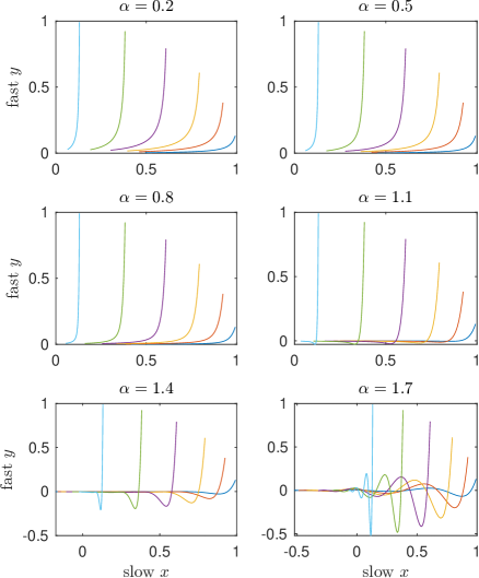
Figure 15: elementary emergence of a slow subspace. Plot six representative trajectories of the ‘multiscale’ fde system in $(x(t),y(t))$: $\partial_{t}^{\alpha}x=-0.03\,x$ and $\partial_{t}^{\alpha}y=-y$. The six subplots are for six different $\alpha\in(0,2)$. The trajectories show, especially for $\alpha\approx 1$, that solutions of the system reasonably quickly reach a neighbourhood of the $x$-axis, the slow subspace $y=0$.

References

- (1)
- Alavi et al. (2023) Alavi, S. E., Ganghoffer, J. F., Reda, H. & Sadighi, M. (2023), ‘Hierarchy of generalized continua issued from micromorphic medium constructed by homogenization’, Continuum Mechanics and Thermodynamics 35(6), 2163–2192.
- Anthoine (2010) Anthoine, A. (2010), ‘Second-order homogenisation of functionally graded materials’, International Journal of Solids and Structures 47(11), 1477–1489.
- Arneodo et al. (1985) Arneodo, A., Coullet, P. H., Spiegel, E. A. & Tresser, C. (1985), ‘Asymptotic chaos’, Physica D 14, 327–347.
- Aulbach & Wanner (2000) Aulbach, B. & Wanner, T. (2000), ‘The Hartman–Grobman theorem for Caratheodory-type differential equations in Banach spaces’, Nonlinear Analysis 40, 91–104.
-
Bates et al. (1998)
Bates, P. W., Lu, K. & Zeng, C. (1998), Existence and persistence of invariant manifolds
for semiflows in Banach space, Vol. 135 of Memoirs Amer. Math. Soc.,
Amer. Math. Soc.
http://books.google.com.au/books?hl=en&lr=&id=mvUHNtSNaaIC&oi=fnd&pg=PA1&dq=related:ctpLfDZOLS4J:scholar.google.com/&ots=3TYgcQ_Jk0&sig=gn6D1qQcsyq51ScDe2LX0HtFWGo#v=onepage&q&f=false - Bažant & Jirásek (2002) Bažant, Z. P. & Jirásek, M. (2002), ‘Nonlocal Integral Formulations of Plasticity and Damage: Survey of Progress’, Journal of Engineering Mechanics 128(11), 1119–1149.
- Bender & Orszag (1981) Bender, C. M. & Orszag, S. A. (1981), Advanced mathematical methods for scientists and engineers: Asymptotic methods and perturbation theory, McGraw–Hill.
- Bokhove & Shepherd (1996) Bokhove, O. & Shepherd, T. G. (1996), ‘On the Hamiltonian balanced dynamics and the slowest invariant manifold’, J. Atmos Sci 53(2), 276–297.
-
Boyd (1995)
Boyd, J. P. (1995), ‘Eight definitions of the
slow manifold: seiches, pseudoseiches and exponential smallness’, Dynamics of Atmospheres and Oceans 22(1–2), 49–75.
http://www.sciencedirect.com/science/article/B6VCR-3YCMH9H-B/2/1a3f0392189659c07097640f3a502dfc - Brenner & Koumoutsakos (2021) Brenner, M. P. & Koumoutsakos, P. (2021), ‘Editorial: Machine Learning and Physical Review Fluids: An Editorial Perspective’, Physical Review Fluids 6(7), 070001.
- Bunder & Roberts (2021) Bunder, J. E. & Roberts, A. J. (2021), ‘Nonlinear emergent macroscale PDEs, with error bound, for nonlinear microscale systems’, Springer Nature Applied Sciences 3(703), 1–28.
-
Carr (1981)
Carr, J. (1981), Applications of centre
manifold theory, Vol. 35 of Applied Math. Sci., Springer–Verlag.
http://books.google.com.au/books?id=93BdN7btysoC - Chekroun et al. (2015) Chekroun, M. D., Liu, H. & Wang, S. (2015), Approximation of Stochastic Invariant Manifolds: Stochastic manifolds for nonlinear SPDEs I, Springer Briefs in Mathematics, Springer, Cham.
-
Chen et al. (2018)
Chen, C., Roberts, A. J. & Bunder, J. E. (2018), ‘Boundary conditions for macroscale waves in an
elastic system with microscale heterogeneity’, IMA Journal of Applied
Mathematics 83(3), 1–33.
http://arxiv.org/abs/1603.06686 - Chen et al. (2024) Chen, D., Gao, K., Yang, J. & Kitipornchai, S. (2024), An introduction to functionally graded porous materials and composite structures, Woodhead Publishing, chapter 1, pp. 3–15.
- Chen et al. (2023) Chen, Y., Hou, T. Y. & Wang, Y. (2023), ‘Exponentially convergent multiscale methods for 2d high frequency heterogeneous helmholtz equations’, Multiscale Modeling & Simulation 21(3), 849–883.
- Chernatynskiy et al. (2013) Chernatynskiy, A., Phillpot, S. R. & LeSar, R. (2013), ‘Uncertainty quantification in multiscale simulation of materials: A prospective’, Annual Review of Materials Research 43(1), 157–182.
- Combescure (2022) Combescure, C. (2022), ‘Selecting Generalized Continuum Theories for Nonlinear Periodic Solids Based on the Instabilities of the Underlying Microstructure’, Journal of Elasticity .
- Cong et al. (2016) Cong, N. D., Doan, T. S., Siegmund, S. & Tuan, H. T. (2016), ‘On stable manifolds for fractional differential equations in high-dimensional spaces’, Nonlinear Dynamics 86(3), 1885–1894.
- Cornaggia & Guzina (2020) Cornaggia, R. & Guzina, B. B. (2020), ‘Second-order homogenization of boundary and transmission conditions for one-dimensional waves in periodic media’, International Journal of Solids and Structures 188–9, 88–102.
- Craster (2015) Craster, R. V. (2015), Dynamic homogenization, in V. V. Mityushev & M. Ruzhansky, eds, ‘Analytic Methods in Interdisciplinary Applications’, Vol. 116 of Springer Proceedings in Mathematics and Statistics, Springer, pp. 41–50.
- Cross & Hohenberg (1993) Cross, M. C. & Hohenberg, P. C. (1993), ‘Pattern formation outside of equilibrium’, Rev. Mod. Phys. 65(3), 851–1112.
- Domb & Sykes (1957) Domb, C. & Sykes, M. F. (1957), ‘On the susceptibility of a ferromagnetic above the Curie point’, Proc. Roy. Soc. Lond. A 240, 214–228.
- Efendiev & Leung (2023) Efendiev, Y. & Leung, W. T. (2023), ‘Multicontinuum homogenization and its relation to nonlocal multicontinuum theories’, Journal of Computational Physics 474(111761), 1–20.
-
Fateman (2003)
Fateman, R. (2003), ‘Comparing the speed of
programs for sparse polynomial multiplication’, ACM SIGSAM Bulletin
37(1), 4–15.
http://www.cs.berkeley.edu/~fateman/papers/fastmult.pdf - Fish et al. (2021) Fish, J., Wagner, G. J. & Keten, S. (2021), ‘Mesoscopic and multiscale modelling in materials’, Nature Materials 20(6), 774–786.
- Forest & Trinh (2011) Forest, S. & Trinh, D. K. (2011), ‘Generalized continua and non-homogeneous boundary conditions in homogenisation methods’, ZAMM—Journal of Applied Mathematics and Mechanics / Zeitschrift für Angewandte Mathematik und Mechanik 91(2), 90–109.
- Frank et al. (2020) Frank, M., Drikakis, D. & Charissis, V. (2020), ‘Machine-learning methods for computational science and engineering’, Computation 8(15), 1–35.
- Golub & van Loan (2013) Golub, G. H. & van Loan, C. F. (2013), Matrix computations, 4th edition edn, John Hopkins University Press.
- Gorenflo & Mainardi (1997) Gorenflo, R. & Mainardi, F. (1997), Fractional calulus: Integral and differential equations of fractional order, in ‘Fractals and Fractional Calculus in Continuum Mechanics’, Vol. 378 of International Centre for Mechanical Sciences, Springer, Vienna.
- Guo et al. (2024) Guo, T., Kouznetsova, V. G., Geers, M. G. D., Veroy, K. & Rokoš, O. (2024), Reduced-order modeling for second-order computational homogenization with applications to geometrically parameterized elastomeric metamaterials, Technical report, arXiv.org.
- Haragus & Iooss (2011) Haragus, M. & Iooss, G. (2011), Local Bifurcations, Center Manifolds, and Normal Forms in Infinite-Dimensional Dynamical Systems, Springer.
- Haubold et al. (2011) Haubold, H. J., Mathai, A. M. & Saxena, R. K. (2011), ‘Mittag-Leffler Functions and Their Applications’, Journal of Applied Mathematics 2011(e298628), 1–51.
- Hii & El Said (2022) Hii, A. K. W. & El Said, B. (2022), ‘A kinematically consistent second-order computational homogenisation framework for thick shell models’, Computer Methods in Applied Mechanics and Engineering 398, 115136.
- Hochs & Roberts (2019) Hochs, P. & Roberts, A. J. (2019), ‘Normal forms and invariant manifolds for nonlinear, non-autonomous PDEs, viewed as ODEs in infinite dimensions’, J. Differential Equations 267(12), 7263–7312.
- Hunter (1987) Hunter, C. (1987), ‘Oscillations in the coefficients of power series’, SIAM J. Appl Math 47, 483–497.
- Jiang et al. (2024) Jiang, K., Li, S. & Zhang, P. (2024), ‘Numerical Methods and Analysis of Computing Quasiperiodic Systems’, SIAM Journal on Numerical Analysis 62(1), 353–375.
- Jiang & Zhang (2014) Jiang, K. & Zhang, P. (2014), ‘Numerical methods for quasicrystals’, Journal of Computational Physics 256, 428–440.
- Leung (2024) Leung, W. T. (2024), Some convergence analysis for multicontinuum homogenization, Technical report, arXiv.org.
- Lorenz (1986) Lorenz, E. N. (1986), ‘On the existence of a slow manifold’, J. Atmos. Sci. 43, 1547–1557.
- Lorenz (1992) Lorenz, E. N. (1992), ‘The slow manifold—what is it?’, Journal of the Atmospheric Sciences 49(24), 2449–2451.
- Lorenz & Krishnamurthy (1987) Lorenz, E. N. & Krishnamurthy, V. (1987), ‘On the non-existence of a slow manifold’, J. Atmos. Sci. 44, 2940–2950.
- Ma & Li (2015) Ma, L. & Li, C. (2015), ‘Center manifold of fractional dynamical system’, Journal of Computational and Nonlinear Dynamics posted 23 July.
-
MacKenzie (2005)
MacKenzie, T. (2005), Create accurate
numerical models of complex spatio-temporal dynamical systems with holistic
discretisation, PhD thesis, University of Southern Queensland.
https://research.usq.edu.au/download/9b26ce2d7d0bd72849b0e3b792cdd4ca16e7991f103845e89e61fa532c9484fe/22666361/Mackenzie_2005_whole.pdf - Martin et al. (2022) Martin, A., Opreni, A., Vizzaccaro, A., Debeurre, M., Salles, L., Frangi, A., Thomas, O. & Touze, C. (2022), Reduced order modeling of geometrically nonlinear rotating structures using the direct parametrisation of invariant manifolds, Technical report, https://hal.archives-ouvertes.fr/hal-03886793.
- Mercer et al. (2015) Mercer, B. S., Mandadapu, K. K. & Papadopoulos, P. (2015), ‘Novel formulations of microscopic boundary-value problems in continuous multiscale finite element methods’, Computer Methods in Applied Mechanics and Engineering 286, 268–292.
- Mercer & Roberts (1990) Mercer, G. N. & Roberts, A. J. (1990), ‘A centre manifold description of contaminant dispersion in channels with varying flow properties’, SIAM J. Appl. Math. 50, 1547–1565.
- Mercer & Roberts (1994) Mercer, G. N. & Roberts, A. J. (1994), ‘A complete model of shear dispersion in pipes’, Jap. J. Indust. Appl. Math. 11, 499–521.
- Muncaster (1983a) Muncaster, R. G. (1983a), ‘Invariant manifolds in mechanics i: The general construction of coarse theories from fine theories’, Arch. Rat. Mech. Anal. 84, 353–373.
- Muncaster (1983b) Muncaster, R. G. (1983b), ‘Invariant manifolds in mechanics ii: Zero-dimensional elastic bodies with directors’, Arch. Rat. Mech. Anal. 84, 375–392.
- Natl Physical Lab (1961) Natl Physical Lab (1961), Modern Computing Methods, Vol. 16 of Notes on Applied Science, 2nd edition edn, Her Majesty’s Stationery Office, London.
- Potzsche & Rasmussen (2006) Potzsche, C. & Rasmussen, M. (2006), ‘Taylor approximation of integral manifolds’, Journal of Dynamics and Differential Equations 18, 427–460.
- Prizzi & Rybakowski (2003) Prizzi, M. & Rybakowski, K. P. (2003), ‘On inertial manifolds for reaction-diffusion equations on genuinely high-dimensional thin domains’, Studia Mathematica 154(3), 253–275.
- Rizzi et al. (2021) Rizzi, G., Hütter, G., Madeo, A. & Neff, P. (2021), ‘Analytical solutions of the simple shear problem for micromorphic models and other generalized continua’, Archive of Applied Mechanics 91(5), 2237–2254.
- Roberts (1988) Roberts, A. J. (1988), ‘The application of centre manifold theory to the evolution of systems which vary slowly in space’, J. Austral. Math. Soc. B 29, 480–500.
- Roberts (1989) Roberts, A. J. (1989), ‘Appropriate initial conditions for asymptotic descriptions of the long term evolution of dynamical systems’, J. Austral. Math. Soc. B 31, 48–75.
- Roberts (1992) Roberts, A. J. (1992), ‘Boundary conditions for approximate differential equations’, J. Austral. Math. Soc. B 34, 54–80.
- Roberts (1993) Roberts, A. J. (1993), ‘The invariant manifold of beam deformations. part 1: the simple circular rod’, J. Elas. 30, 1–54.
- Roberts (1996) Roberts, A. J. (1996), ‘Low-dimensional models of thin film fluid dynamics’, Phys. Letts. A 212, 63–72.
- Roberts (1997) Roberts, A. J. (1997), ‘Low-dimensional modelling of dynamics via computer algebra’, Computer Phys. Comm. 100, 215–230.
- Roberts (2000) Roberts, A. J. (2000), ‘Computer algebra derives correct initial conditions for low-dimensional dynamical models’, Computer Phys. Comm. 126(3), 187–206.
- Roberts (2015a) Roberts, A. J. (2015a), ‘Macroscale, slowly varying, models emerge from the microscale dynamics in long thin domains’, IMA Journal of Applied Mathematics 80(5), 1492–1518.
-
Roberts (2015b)
Roberts, A. J. (2015b), Model
emergent dynamics in complex systems, SIAM, Philadelphia.
https://epubs.siam.org/doi/10.1137/1.9781611973563 - Roberts (2021) Roberts, A. J. (2021), Rigorous modelling of nonlocal interactions determines a macroscale advection-diffusion PDE, in D. R. Wood, J. d. Gier, C. E. Praeger & T. Tao, eds, ‘2019-20 MATRIX Annals’, MATRIX Book Series, Springer International Publishing, pp. 423–437.
- Roberts (2022) Roberts, A. J. (2022), Backwards theory supports modelling via invariant manifolds for non-autonomous dynamical systems, Technical report, [http://arxiv.org/abs/1804.06998].
- Roberts (2024) Roberts, A. J. (2024), ‘Embed in ensemble to rigorously and accurately homogenise quasi-periodic multi-scale heterogeneous material’, ANZIAM Journal accepted 08-Mar-2024.
-
Roberts & Bunder (2017)
Roberts, A. J. & Bunder, J. E. (2017), ‘Slowly varying, macroscale models emerge from
microscale dynamics over multiscale domains’, IMA Journal of Applied
Mathematics 82, 971–1012.
http://arxiv.org/abs/1612.02079 - Roberts & Li (2006) Roberts, A. J. & Li, Z. (2006), ‘An accurate and comprehensive model of thin fluid flows with inertia on curved substrates’, J. Fluid Mech. 553, 33–73.
- Roberts et al. (2014) Roberts, A. J., MacKenzie, T. & Bunder, J. (2014), ‘A dynamical systems approach to simulating macroscale spatial dynamics in multiple dimensions’, J. Engineering Mathematics 86(1), 175–207.
- Roberts & Strunin (2004) Roberts, A. J. & Strunin, D. V. (2004), ‘Two-zone model of shear dispersion in a channel using centre manifolds’, Quart. J. Mech. Appl. Math. 57, 363–378.
- Rokoš et al. (2019) Rokoš, O., Ameen, M. M., Peerlings, R. H. J. & Geers, M. G. D. (2019), ‘Micromorphic computational homogenization for mechanical metamaterials with patterning fluctuation fields’, Journal of the Mechanics and Physics of Solids 123, 119–137.
-
Rosencrans (1997)
Rosencrans, S. (1997), ‘Taylor dispersion in
curved channels’, SIAM J. Appl. Math. 57, 1216–1241.
http://www.jstor.org/stable/2951850 - Sanderse et al. (2024) Sanderse, B., Stinis, P., Maulik, R. & Ahmed, S. E. (2024), Scientific machine learning for closure models in multiscale problems: a review, Technical report, arXiv.org.
- Sarhil et al. (2024) Sarhil, M., Scheunemann, L., Lewintan, P., Schröder, J. & Neff, P. (2024), A computational approach to identify the material parameters of the relaxed micromorphic model, Technical report, arXiv.org.
- Siettos & Russo (2021) Siettos, C. & Russo, L. (2021), ‘A numerical method for the approximation of stable and unstable manifolds of microscopic simulators’, Numerical Algorithms .
- Sijbrand (1985) Sijbrand, J. (1985), ‘Properties of center manifolds’, Trans. Amer. Math. Soc. 289(2), 431–469.
- Somnic & Jo (2022) Somnic, J. & Jo, B. W. (2022), ‘Status and challenges in homogenization methods for lattice materials’, Materials 15(2), 605.
- Suslov & Roberts (1999) Suslov, S. A. & Roberts, A. J. (1999), ‘Advection-dispersion in symmetric field-flow fractionation channels’, J. Math. Chem. 26, 27–46.
- Suslov & Roberts (2000) Suslov, S. A. & Roberts, A. J. (2000), ‘Modelling of sample dynamics in rectangular asymmetrical flow field-flow fractionation channels’, Analytical Chemistry 72(18), 4331–4345.
- Touze & Amabili (2006) Touze, C. & Amabili, M. (2006), ‘Nonlinear normal modes for damped geometrically nonlinear systems: Application to reduced-order modelling of harmonically forced structures’, J. Sound & Vibration 298(4–5), 958–981.
- Touzé & Vizzaccaro (2021) Touzé, C. & Vizzaccaro, A. (2021), ‘Model order reduction methods for geometrically nonlinear structures: a review of nonlinear techniques’, Nonlinear Dynamics 105(2), 1141–1190.
- van Kampen (1985) van Kampen, N. G. (1985), ‘Elimination of fast variables’, Physics Reports 124, 69–160.
- Vanneste & Yavneh (2004) Vanneste, J. & Yavneh, I. (2004), ‘Exponentially small inertia-gravity waves and the breakdown of quasigeostrophic balance’, J. Atmos. Sci. 61, 211–223.
- Wanga et al. (2024) Wanga, F., Wang, Y., Leung, W. T. & Xu, Z. (2024), Learning-based multi-continuum model for multiscale flow problems, Technical report, arXiv.org.
- Watt & Roberts (1995) Watt, S. D. & Roberts, A. J. (1995), ‘The accurate dynamic modelling of contaminant dispersion in channels’, SIAM J. Appl. Math. 55(4), 1016–1038.