\tikzfeynmanset

warn luatex=false \tikzfeynmanset with arrow/.style = decoration= markings, mark=at position 0.5 with \arrow[xshift=0.4mm]Stealth[black,width=1mm,length=1.3mm] , postaction=decorate \tikzfeynmanset yourboson/.style= decorate, decoration= snake, mirror, amplitude=0.6mm, segment length=2.16mm, pre, pre length=0pt, post, post length=0pt institutetext: Department of Physics, Baylor University, One Bear Place #97316, Waco, TX 76798-7316

EFT at JADE: a case study

Jonathan S. Wilson Jon_Wilson2@baylor.edu
Abstract

As we use the standard model effective field theory to search for signs of new physics beyond the reach of the LHC, we often wonder what we may learn from the effective field theory, and what it would look like to make a discovery via effective field theory. This article presents a case study that provides some answers to these questions. We apply the low-energy effective field theory to ${\mathit{{{\mathit{{e}{}_{\mspace{-3.0mu}\scriptstyle{}}^{\mspace{-1.0mu}\scriptstyle{}}}}}{}_{\mspace{-3.0mu}\scriptstyle{}}^{\mspace{-1.0mu}\scriptstyle{+}}}}{\mathit{{{\mathit{{e}{}_{\mspace{-3.0mu}\scriptstyle{}}^{\mspace{-1.0mu}\scriptstyle{}}}}}{}_{\mspace{-3.0mu}\scriptstyle{}}^{\mspace{-1.0mu}\scriptstyle{-}}}}\to{\mathit{{{\mathit{{\upmu}{}_{\mspace{-3.0mu}\scriptstyle{}}^{\mspace{-1.0mu}\scriptstyle{}}}}}{}_{\mspace{-3.0mu}\scriptstyle{}}^{\mspace{-1.0mu}\scriptstyle{+}}}}{\mathit{{{\mathit{{\upmu}{}_{\mspace{-3.0mu}\scriptstyle{}}^{\mspace{-1.0mu}\scriptstyle{}}}}}{}_{\mspace{-3.0mu}\scriptstyle{}}^{\mspace{-1.0mu}\scriptstyle{-}}}}$ data below the $\mathit{{Z}{}_{\mspace{-3.0mu}\scriptstyle{}}^{\mspace{-1.0mu}\scriptstyle{}}}$ boson mass from the JADE experiment at DESY. The low-energy effective field theory allows the observation of physics beyond QED in the JADE data and furthermore, by matching the Wilson coefficients to the electroweak theory, a rough measurement of the masses of the $\mathit{{W}{}_{\mspace{-3.0mu}\scriptstyle{}}^{\mspace{-1.0mu}\scriptstyle{}}}$ and $\mathit{{Z}{}_{\mspace{-3.0mu}\scriptstyle{}}^{\mspace{-1.0mu}\scriptstyle{}}}$ bosons is possible. This rough measurement would have been sufficient to guide the construction of colliders such as the super proton-antiproton synchrotron or the large electron-positron collider, and so we anticipate that a discovery of new physics via effective field theory at the LHC would be similarly sufficient to guide the construction of future colliders.

1 Introduction

The LHC today boasts a robust program searching for signs of physics beyond the standard model (SM) using the SM effective field theory (SMEFT) Ethier:2021bye . The question of what an observation of new physics via SMEFT would teach us is often raised, and the response is generally that, without more targeted data analysis and probably a higher-energy experiment, we will not be able to learn anything about the new physics beyond its existence, not even the energy scale of the new physics.

We have performed a case study that challenges this assumption. By examining data from below the $\mathit{{Z}{}_{\mspace{-3.0mu}\scriptstyle{}}^{\mspace{-1.0mu}\scriptstyle{}}}$ boson mass using the low-energy effective field theory (LEFT) and matching the LEFT Wilson coefficients to the electroweak theory, we show that substantial knowledge about the energy scale of new physics can be obtained.

This case study uses ${\mathit{{{\mathit{{e}{}_{\mspace{-3.0mu}\scriptstyle{}}^{\mspace{-1.0mu}\scriptstyle{}}}}}{}_{\mspace{-3.0mu}\scriptstyle{}}^{\mspace{-1.0mu}\scriptstyle{+}}}}{\mathit{{{\mathit{{e}{}_{\mspace{-3.0mu}\scriptstyle{}}^{\mspace{-1.0mu}\scriptstyle{}}}}}{}_{\mspace{-3.0mu}\scriptstyle{}}^{\mspace{-1.0mu}\scriptstyle{-}}}}\to{\mathit{{{\mathit{{\upmu}{}_{\mspace{-3.0mu}\scriptstyle{}}^{\mspace{-1.0mu}\scriptstyle{}}}}}{}_{\mspace{-3.0mu}\scriptstyle{}}^{\mspace{-1.0mu}\scriptstyle{+}}}}{\mathit{{{\mathit{{\upmu}{}_{\mspace{-3.0mu}\scriptstyle{}}^{\mspace{-1.0mu}\scriptstyle{}}}}}{}_{\mspace{-3.0mu}\scriptstyle{}}^{\mspace{-1.0mu}\scriptstyle{-}}}}$ data from the JADE experiment at DESY, and ignores all of the other data relevant to electroweak effects that was available at the time. It is therefore a counter-historical case study but it more closely mimics a hypothetical future in which indications of physics beyond the SM have been observed at the LHC via SMEFT measurements.

We describe the JADE data in section 2, the LEFT and its predictions in section 3, the fit to the JADE data to measure the LEFT Wilson coefficients in section 4, the matching of the LEFT Wilson coefficients to the electroweak theory predictions in section 5, and the measurement of the masses of the $\mathit{{W}{}_{\mspace{-3.0mu}\scriptstyle{}}^{\mspace{-1.0mu}\scriptstyle{}}}$ and $\mathit{{Z}{}_{\mspace{-3.0mu}\scriptstyle{}}^{\mspace{-1.0mu}\scriptstyle{}}}$ bosons in section 6.

2 Data

The JADE (JApan, Deutschland, and England) experiment at the PETRA particle accelerator at DESY was a general-purpose particle detector NAROSKA198767 . It recorded $e^{+}e^{-}$ collisions from 1979 to 1986, with center-of-mass energies ranging from 12 to $46.6\text{\,}\mathrm{GeV}$.

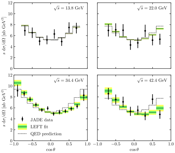
JADE measures the differential cross section for electron-positron annihilation at a pair of muons as a function of the angle, in the center-of-mass frame, between the incoming electron and outgoing muon momenta JADE_mu_AFB . This measurement is performed at four center-of-mass energies: 13.8, 22.0, 34.4, and $42.4\text{\,}\mathrm{GeV}$. A forward-backward asymmetry is observed, which increases with center-of-mass energy and is consistent with the predictions of the electroweak theory.

The differential cross section, multiplied by the Mandelstam variable $s$ and divided by the bin width, is measured in several bins of $\cos\theta$, as shown in tables 1 and 2 as well as figure 2 of ref. JADE_mu_AFB . The binning depends on the center-of-mass energy at which the measurement is performed.

Bin Bin width $w$ $\left(s/w\right)\left(\mathrm{d}\sigma/\mathrm{d}\cos\theta\right)$ [$\mathrm{nb}\text{\,}{\mathrm{GeV}}^{2}$]
$13.8\text{\,}\mathrm{GeV}$ $22.0\text{\,}\mathrm{GeV}$ $42.4\text{\,}\mathrm{GeV}$
$(-0.8,-0.6)$ 0.2 $6.91\pm 0.93$ $6.95\pm 1.11$ $8.58\pm 1.06$
$(-0.6,-0.4)$ 0.2 $6.53\pm 0.95$ $7.06\pm 1.17$ $7.53\pm 0.90$
$(-0.4,-0.2)$ 0.2 $5.00\pm 0.76$ $6.99\pm 1.11$ $7.10\pm 0.94$
$(-0.2,\phantom{-}0.0)$ 0.2 $5.23\pm 0.80$ $4.29\pm 0.88$ $5.37\pm 0.83$
$(\phantom{-}0.0,\phantom{-}0.2)$ 0.2 $6.30\pm 0.85$ $4.68\pm 0.95$ $5.57\pm 0.83$
$(\phantom{-}0.2,\phantom{-}0.4)$ 0.2 $4.92\pm 0.79$ $6.87\pm 1.12$ $4.54\pm 0.78$
$(\phantom{-}0.4,\phantom{-}0.6)$ 0.2 $7.49\pm 0.94$ $5.17\pm 0.94$ $7.57\pm 0.91$
$(\phantom{-}0.6,\phantom{-}0.8)$ 0.2 $7.37\pm 0.96$ $5.34\pm 0.99$ $4.81\pm 0.79$
Table 1: The JADE measurement of the differential cross section $\left(s/w\right)\left(\mathrm{d}\sigma/\mathrm{d}\cos\theta\right)$, where $w$ is the bin width, in several bins at center-of-mass energies of 13.8, 22.0, and $42.4\text{\,}\mathrm{GeV}$.
Bin Bin width $w$ $\left(s/w\right)\left(\mathrm{d}\sigma/\mathrm{d}\cos\theta\right)$ [$\mathrm{nb}\text{\,}{\mathrm{GeV}}^{2}$]
$(-1.00,-0.80)$ 0.20 $9.15\pm 1.10$
$(-0.80,-0.64)$ 0.16 $8.56\pm 0.47$
$(-0.64,-0.48)$ 0.16 $7.57\pm 0.45$
$(-0.48,-0.32)$ 0.16 $6.58\pm 0.38$
$(-0.32,-0.16)$ 0.16 $5.62\pm 0.33$
$(-0.16,\phantom{-}0.00)$ 0.16 $5.93\pm 0.37$
$(\phantom{-}0.00,\phantom{-}0.16)$ 0.16 $4.91\pm 0.36$
$(\phantom{-}0.16,\phantom{-}0.32)$ 0.16 $5.24\pm 0.41$
$(\phantom{-}0.32,\phantom{-}0.48)$ 0.16 $5.40\pm 0.36$
$(\phantom{-}0.48,\phantom{-}0.64)$ 0.16 $5.84\pm 0.39$
$(\phantom{-}0.64,\phantom{-}0.80)$ 0.16 $6.30\pm 0.40$
$(\phantom{-}0.80,\phantom{-}1.00)$ 0.20 $8.30\pm 1.04$
Table 2: The JADE measurement of the differential cross section $\left(s/w\right)\left(\mathrm{d}\sigma/\mathrm{d}\cos\theta\right)$, where $w$ is the bin width, in several bins at a center-of-mass energy of $34.4\text{\,}\mathrm{GeV}$.

3 The low-energy effective field theory

The low-energy effective field theory (LEFT) LEFT describes physics below the electroweak scale. The $\mathit{{W}{}_{\mspace{-3.0mu}\scriptstyle{}}^{\mspace{-1.0mu}\scriptstyle{}}}$, $\mathit{{Z}{}_{\mspace{-3.0mu}\scriptstyle{}}^{\mspace{-1.0mu}\scriptstyle{}}}$, and Higgs bosons and the top quark are integrated out of the SMEFT to obtain the LEFT. In the most general flavor assumptions, this produces a total of 6083 operators, including dimensions 3, 5, and 6 and allowing CP violation. If we restrict ourselves to only operators that affect ${\mathit{{{\mathit{{e}{}_{\mspace{-3.0mu}\scriptstyle{}}^{\mspace{-1.0mu}\scriptstyle{}}}}}{}_{\mspace{-3.0mu}\scriptstyle{}}^{\mspace{-1.0mu}\scriptstyle{+}}}}{\mathit{{{\mathit{{e}{}_{\mspace{-3.0mu}\scriptstyle{}}^{\mspace{-1.0mu}\scriptstyle{}}}}}{}_{\mspace{-3.0mu}\scriptstyle{}}^{\mspace{-1.0mu}\scriptstyle{-}}}}\to{\mathit{{{\mathit{{\upmu}{}_{\mspace{-3.0mu}\scriptstyle{}}^{\mspace{-1.0mu}\scriptstyle{}}}}}{}_{\mspace{-3.0mu}\scriptstyle{}}^{\mspace{-1.0mu}\scriptstyle{+}}}}{\mathit{{{\mathit{{\upmu}{}_{\mspace{-3.0mu}\scriptstyle{}}^{\mspace{-1.0mu}\scriptstyle{}}}}}{}_{\mspace{-3.0mu}\scriptstyle{}}^{\mspace{-1.0mu}\scriptstyle{-}}}}$ at tree level and do not produce CP violation, there are 14 operators, which are listed in table 3. Further restricting to only those operators that have nonzero Wilson coefficients in the SM leaves only 4 contributions, all at dimension 6: $C^{V,LL}_{\begin{subarray}{c}ee\\ {\mathit{{e}{}_{\mspace{-3.0mu}\scriptstyle{}}^{\mspace{-1.0mu}\scriptstyle{}}}}{\mathit{{e}{}_{\mspace{-3.0mu}\scriptstyle{}}^{\mspace{-1.0mu}\scriptstyle{}}}}{\mathit{{\upmu}{}_{\mspace{-3.0mu}\scriptstyle{}}^{\mspace{-1.0mu}\scriptstyle{}}}}{\mathit{{\upmu}{}_{\mspace{-3.0mu}\scriptstyle{}}^{\mspace{-1.0mu}\scriptstyle{}}}}\end{subarray}}$, $C^{V,RR}_{\begin{subarray}{c}ee\\ {\mathit{{e}{}_{\mspace{-3.0mu}\scriptstyle{}}^{\mspace{-1.0mu}\scriptstyle{}}}}{\mathit{{e}{}_{\mspace{-3.0mu}\scriptstyle{}}^{\mspace{-1.0mu}\scriptstyle{}}}}{\mathit{{\upmu}{}_{\mspace{-3.0mu}\scriptstyle{}}^{\mspace{-1.0mu}\scriptstyle{}}}}{\mathit{{\upmu}{}_{\mspace{-3.0mu}\scriptstyle{}}^{\mspace{-1.0mu}\scriptstyle{}}}}\end{subarray}}$, $C^{V,LR}_{\begin{subarray}{c}ee\\ {\mathit{{e}{}_{\mspace{-3.0mu}\scriptstyle{}}^{\mspace{-1.0mu}\scriptstyle{}}}}{\mathit{{e}{}_{\mspace{-3.0mu}\scriptstyle{}}^{\mspace{-1.0mu}\scriptstyle{}}}}{\mathit{{\upmu}{}_{\mspace{-3.0mu}\scriptstyle{}}^{\mspace{-1.0mu}\scriptstyle{}}}}{\mathit{{\upmu}{}_{\mspace{-3.0mu}\scriptstyle{}}^{\mspace{-1.0mu}\scriptstyle{}}}}\end{subarray}}$, and $C^{V,LR}_{\begin{subarray}{c}ee\\ {\mathit{{\upmu}{}_{\mspace{-3.0mu}\scriptstyle{}}^{\mspace{-1.0mu}\scriptstyle{}}}}{\mathit{{\upmu}{}_{\mspace{-3.0mu}\scriptstyle{}}^{\mspace{-1.0mu}\scriptstyle{}}}}{\mathit{{e}{}_{\mspace{-3.0mu}\scriptstyle{}}^{\mspace{-1.0mu}\scriptstyle{}}}}{\mathit{{e}{}_{\mspace{-3.0mu}\scriptstyle{}}^{\mspace{-1.0mu}\scriptstyle{}}}}\end{subarray}}$, which we will write as $C^{LL}$, $C^{RR}$, $C^{LR}$, and $C^{RL}$, respectively, for the sake of brevity.

Wilson coefficient Flavor indices Operator definition Nonzero in SM
$C_{\begin{subarray}{c}{\mathit{{e}{}_{\mspace{-3.0mu}\scriptstyle{}}^{\mspace{-1.0mu}\scriptstyle{}}}}{\mathit{{\upgamma}{}_{\mspace{-3.0mu}\scriptstyle{}}^{\mspace{-1.0mu}\scriptstyle{}}}}\\ pr\end{subarray}}$ $pr={\mathit{{e}{}_{\mspace{-3.0mu}\scriptstyle{}}^{\mspace{-1.0mu}\scriptstyle{}}}}{\mathit{{e}{}_{\mspace{-3.0mu}\scriptstyle{}}^{\mspace{-1.0mu}\scriptstyle{}}}}$ $\overline{{\mathit{{e}{}_{\mspace{-3.0mu}\scriptstyle{}}^{\mspace{-1.0mu}\scriptstyle{}}}}}_{Lp}\sigma^{\mu\nu}{\mathit{{e}{}_{\mspace{-3.0mu}\scriptstyle{}}^{\mspace{-1.0mu}\scriptstyle{}}}}_{Rr}F_{\mu\nu}$
$C_{\begin{subarray}{c}{\mathit{{e}{}_{\mspace{-3.0mu}\scriptstyle{}}^{\mspace{-1.0mu}\scriptstyle{}}}}{\mathit{{\upgamma}{}_{\mspace{-3.0mu}\scriptstyle{}}^{\mspace{-1.0mu}\scriptstyle{}}}}\\ pr\end{subarray}}$ $pr={\mathit{{\upmu}{}_{\mspace{-3.0mu}\scriptstyle{}}^{\mspace{-1.0mu}\scriptstyle{}}}}{\mathit{{\upmu}{}_{\mspace{-3.0mu}\scriptstyle{}}^{\mspace{-1.0mu}\scriptstyle{}}}}$ $\overline{{\mathit{{e}{}_{\mspace{-3.0mu}\scriptstyle{}}^{\mspace{-1.0mu}\scriptstyle{}}}}}_{Lp}\sigma^{\mu\nu}{\mathit{{e}{}_{\mspace{-3.0mu}\scriptstyle{}}^{\mspace{-1.0mu}\scriptstyle{}}}}_{Rr}F_{\mu\nu}$
$C_{\begin{subarray}{c}{\mathit{{e}{}_{\mspace{-3.0mu}\scriptstyle{}}^{\mspace{-1.0mu}\scriptstyle{}}}}{\mathit{{\upgamma}{}_{\mspace{-3.0mu}\scriptstyle{}}^{\mspace{-1.0mu}\scriptstyle{}}}}\\ pr\end{subarray}}$ $pr={\mathit{{e}{}_{\mspace{-3.0mu}\scriptstyle{}}^{\mspace{-1.0mu}\scriptstyle{}}}}{\mathit{{\upmu}{}_{\mspace{-3.0mu}\scriptstyle{}}^{\mspace{-1.0mu}\scriptstyle{}}}}$ $\overline{{\mathit{{e}{}_{\mspace{-3.0mu}\scriptstyle{}}^{\mspace{-1.0mu}\scriptstyle{}}}}}_{Lp}\sigma^{\mu\nu}{\mathit{{e}{}_{\mspace{-3.0mu}\scriptstyle{}}^{\mspace{-1.0mu}\scriptstyle{}}}}_{Rr}F_{\mu\nu}$
$C_{\begin{subarray}{c}{\mathit{{e}{}_{\mspace{-3.0mu}\scriptstyle{}}^{\mspace{-1.0mu}\scriptstyle{}}}}{\mathit{{\upgamma}{}_{\mspace{-3.0mu}\scriptstyle{}}^{\mspace{-1.0mu}\scriptstyle{}}}}\\ pr\end{subarray}}$ $pr={\mathit{{\upmu}{}_{\mspace{-3.0mu}\scriptstyle{}}^{\mspace{-1.0mu}\scriptstyle{}}}}{\mathit{{e}{}_{\mspace{-3.0mu}\scriptstyle{}}^{\mspace{-1.0mu}\scriptstyle{}}}}$ $\overline{{\mathit{{e}{}_{\mspace{-3.0mu}\scriptstyle{}}^{\mspace{-1.0mu}\scriptstyle{}}}}}_{Lp}\sigma^{\mu\nu}{\mathit{{e}{}_{\mspace{-3.0mu}\scriptstyle{}}^{\mspace{-1.0mu}\scriptstyle{}}}}_{Rr}F_{\mu\nu}$
$C^{V,LL}_{\begin{subarray}{c}{\mathit{{e}{}_{\mspace{-3.0mu}\scriptstyle{}}^{\mspace{-1.0mu}\scriptstyle{}}}}{\mathit{{e}{}_{\mspace{-3.0mu}\scriptstyle{}}^{\mspace{-1.0mu}\scriptstyle{}}}}\\ prst\end{subarray}}$ $prst={\mathit{{e}{}_{\mspace{-3.0mu}\scriptstyle{}}^{\mspace{-1.0mu}\scriptstyle{}}}}{\mathit{{e}{}_{\mspace{-3.0mu}\scriptstyle{}}^{\mspace{-1.0mu}\scriptstyle{}}}}{\mathit{{\upmu}{}_{\mspace{-3.0mu}\scriptstyle{}}^{\mspace{-1.0mu}\scriptstyle{}}}}{\mathit{{\upmu}{}_{\mspace{-3.0mu}\scriptstyle{}}^{\mspace{-1.0mu}\scriptstyle{}}}}$ $\left(\overline{{\mathit{{e}{}_{\mspace{-3.0mu}\scriptstyle{}}^{\mspace{-1.0mu}\scriptstyle{}}}}}_{Lp}\gamma^{\mu}{\mathit{{e}{}_{\mspace{-3.0mu}\scriptstyle{}}^{\mspace{-1.0mu}\scriptstyle{}}}}_{Lr}\right)\left(\overline{{\mathit{{e}{}_{\mspace{-3.0mu}\scriptstyle{}}^{\mspace{-1.0mu}\scriptstyle{}}}}}_{Ls}\gamma_{\mu}{\mathit{{e}{}_{\mspace{-3.0mu}\scriptstyle{}}^{\mspace{-1.0mu}\scriptstyle{}}}}_{Lt}\right)$ *
$C^{V,LL}_{\begin{subarray}{c}{\mathit{{e}{}_{\mspace{-3.0mu}\scriptstyle{}}^{\mspace{-1.0mu}\scriptstyle{}}}}{\mathit{{e}{}_{\mspace{-3.0mu}\scriptstyle{}}^{\mspace{-1.0mu}\scriptstyle{}}}}\\ prst\end{subarray}}$ $prst={\mathit{{e}{}_{\mspace{-3.0mu}\scriptstyle{}}^{\mspace{-1.0mu}\scriptstyle{}}}}{\mathit{{\upmu}{}_{\mspace{-3.0mu}\scriptstyle{}}^{\mspace{-1.0mu}\scriptstyle{}}}}{\mathit{{\upmu}{}_{\mspace{-3.0mu}\scriptstyle{}}^{\mspace{-1.0mu}\scriptstyle{}}}}{\mathit{{e}{}_{\mspace{-3.0mu}\scriptstyle{}}^{\mspace{-1.0mu}\scriptstyle{}}}}$ $\left(\overline{{\mathit{{e}{}_{\mspace{-3.0mu}\scriptstyle{}}^{\mspace{-1.0mu}\scriptstyle{}}}}}_{Lp}\gamma^{\mu}{\mathit{{e}{}_{\mspace{-3.0mu}\scriptstyle{}}^{\mspace{-1.0mu}\scriptstyle{}}}}_{Lr}\right)\left(\overline{{\mathit{{e}{}_{\mspace{-3.0mu}\scriptstyle{}}^{\mspace{-1.0mu}\scriptstyle{}}}}}_{Ls}\gamma_{\mu}{\mathit{{e}{}_{\mspace{-3.0mu}\scriptstyle{}}^{\mspace{-1.0mu}\scriptstyle{}}}}_{Lt}\right)$
$C^{V,RR}_{\begin{subarray}{c}{\mathit{{e}{}_{\mspace{-3.0mu}\scriptstyle{}}^{\mspace{-1.0mu}\scriptstyle{}}}}{\mathit{{e}{}_{\mspace{-3.0mu}\scriptstyle{}}^{\mspace{-1.0mu}\scriptstyle{}}}}\\ prst\end{subarray}}$ $prst={\mathit{{e}{}_{\mspace{-3.0mu}\scriptstyle{}}^{\mspace{-1.0mu}\scriptstyle{}}}}{\mathit{{e}{}_{\mspace{-3.0mu}\scriptstyle{}}^{\mspace{-1.0mu}\scriptstyle{}}}}{\mathit{{\upmu}{}_{\mspace{-3.0mu}\scriptstyle{}}^{\mspace{-1.0mu}\scriptstyle{}}}}{\mathit{{\upmu}{}_{\mspace{-3.0mu}\scriptstyle{}}^{\mspace{-1.0mu}\scriptstyle{}}}}$ $\left(\overline{{\mathit{{e}{}_{\mspace{-3.0mu}\scriptstyle{}}^{\mspace{-1.0mu}\scriptstyle{}}}}}_{Rp}\gamma^{\mu}{\mathit{{e}{}_{\mspace{-3.0mu}\scriptstyle{}}^{\mspace{-1.0mu}\scriptstyle{}}}}_{Rr}\right)\left(\overline{{\mathit{{e}{}_{\mspace{-3.0mu}\scriptstyle{}}^{\mspace{-1.0mu}\scriptstyle{}}}}}_{Rs}\gamma_{\mu}{\mathit{{e}{}_{\mspace{-3.0mu}\scriptstyle{}}^{\mspace{-1.0mu}\scriptstyle{}}}}_{Rt}\right)$ *
$C^{V,RR}_{\begin{subarray}{c}{\mathit{{e}{}_{\mspace{-3.0mu}\scriptstyle{}}^{\mspace{-1.0mu}\scriptstyle{}}}}{\mathit{{e}{}_{\mspace{-3.0mu}\scriptstyle{}}^{\mspace{-1.0mu}\scriptstyle{}}}}\\ prst\end{subarray}}$ $prst={\mathit{{e}{}_{\mspace{-3.0mu}\scriptstyle{}}^{\mspace{-1.0mu}\scriptstyle{}}}}{\mathit{{\upmu}{}_{\mspace{-3.0mu}\scriptstyle{}}^{\mspace{-1.0mu}\scriptstyle{}}}}{\mathit{{\upmu}{}_{\mspace{-3.0mu}\scriptstyle{}}^{\mspace{-1.0mu}\scriptstyle{}}}}{\mathit{{e}{}_{\mspace{-3.0mu}\scriptstyle{}}^{\mspace{-1.0mu}\scriptstyle{}}}}$ $\left(\overline{{\mathit{{e}{}_{\mspace{-3.0mu}\scriptstyle{}}^{\mspace{-1.0mu}\scriptstyle{}}}}}_{Rp}\gamma^{\mu}{\mathit{{e}{}_{\mspace{-3.0mu}\scriptstyle{}}^{\mspace{-1.0mu}\scriptstyle{}}}}_{Rr}\right)\left(\overline{{\mathit{{e}{}_{\mspace{-3.0mu}\scriptstyle{}}^{\mspace{-1.0mu}\scriptstyle{}}}}}_{Rs}\gamma_{\mu}{\mathit{{e}{}_{\mspace{-3.0mu}\scriptstyle{}}^{\mspace{-1.0mu}\scriptstyle{}}}}_{Rt}\right)$
$C^{V,LR}_{\begin{subarray}{c}{\mathit{{e}{}_{\mspace{-3.0mu}\scriptstyle{}}^{\mspace{-1.0mu}\scriptstyle{}}}}{\mathit{{e}{}_{\mspace{-3.0mu}\scriptstyle{}}^{\mspace{-1.0mu}\scriptstyle{}}}}\\ prst\end{subarray}}$ $prst={\mathit{{e}{}_{\mspace{-3.0mu}\scriptstyle{}}^{\mspace{-1.0mu}\scriptstyle{}}}}{\mathit{{e}{}_{\mspace{-3.0mu}\scriptstyle{}}^{\mspace{-1.0mu}\scriptstyle{}}}}{\mathit{{\upmu}{}_{\mspace{-3.0mu}\scriptstyle{}}^{\mspace{-1.0mu}\scriptstyle{}}}}{\mathit{{\upmu}{}_{\mspace{-3.0mu}\scriptstyle{}}^{\mspace{-1.0mu}\scriptstyle{}}}}$ $\left(\overline{{\mathit{{e}{}_{\mspace{-3.0mu}\scriptstyle{}}^{\mspace{-1.0mu}\scriptstyle{}}}}}_{Lp}\gamma^{\mu}{\mathit{{e}{}_{\mspace{-3.0mu}\scriptstyle{}}^{\mspace{-1.0mu}\scriptstyle{}}}}_{Lr}\right)\left(\overline{{\mathit{{e}{}_{\mspace{-3.0mu}\scriptstyle{}}^{\mspace{-1.0mu}\scriptstyle{}}}}}_{Rs}\gamma_{\mu}{\mathit{{e}{}_{\mspace{-3.0mu}\scriptstyle{}}^{\mspace{-1.0mu}\scriptstyle{}}}}_{Rt}\right)$ *
$C^{V,LR}_{\begin{subarray}{c}{\mathit{{e}{}_{\mspace{-3.0mu}\scriptstyle{}}^{\mspace{-1.0mu}\scriptstyle{}}}}{\mathit{{e}{}_{\mspace{-3.0mu}\scriptstyle{}}^{\mspace{-1.0mu}\scriptstyle{}}}}\\ prst\end{subarray}}$ $prst={\mathit{{\upmu}{}_{\mspace{-3.0mu}\scriptstyle{}}^{\mspace{-1.0mu}\scriptstyle{}}}}{\mathit{{\upmu}{}_{\mspace{-3.0mu}\scriptstyle{}}^{\mspace{-1.0mu}\scriptstyle{}}}}{\mathit{{e}{}_{\mspace{-3.0mu}\scriptstyle{}}^{\mspace{-1.0mu}\scriptstyle{}}}}{\mathit{{e}{}_{\mspace{-3.0mu}\scriptstyle{}}^{\mspace{-1.0mu}\scriptstyle{}}}}$ $\left(\overline{{\mathit{{e}{}_{\mspace{-3.0mu}\scriptstyle{}}^{\mspace{-1.0mu}\scriptstyle{}}}}}_{Lp}\gamma^{\mu}{\mathit{{e}{}_{\mspace{-3.0mu}\scriptstyle{}}^{\mspace{-1.0mu}\scriptstyle{}}}}_{Lr}\right)\left(\overline{{\mathit{{e}{}_{\mspace{-3.0mu}\scriptstyle{}}^{\mspace{-1.0mu}\scriptstyle{}}}}}_{Rs}\gamma_{\mu}{\mathit{{e}{}_{\mspace{-3.0mu}\scriptstyle{}}^{\mspace{-1.0mu}\scriptstyle{}}}}_{Rt}\right)$ *
$C^{V,LR}_{\begin{subarray}{c}{\mathit{{e}{}_{\mspace{-3.0mu}\scriptstyle{}}^{\mspace{-1.0mu}\scriptstyle{}}}}{\mathit{{e}{}_{\mspace{-3.0mu}\scriptstyle{}}^{\mspace{-1.0mu}\scriptstyle{}}}}\\ prst\end{subarray}}$ $prst={\mathit{{e}{}_{\mspace{-3.0mu}\scriptstyle{}}^{\mspace{-1.0mu}\scriptstyle{}}}}{\mathit{{\upmu}{}_{\mspace{-3.0mu}\scriptstyle{}}^{\mspace{-1.0mu}\scriptstyle{}}}}{\mathit{{\upmu}{}_{\mspace{-3.0mu}\scriptstyle{}}^{\mspace{-1.0mu}\scriptstyle{}}}}{\mathit{{e}{}_{\mspace{-3.0mu}\scriptstyle{}}^{\mspace{-1.0mu}\scriptstyle{}}}}$ $\left(\overline{{\mathit{{e}{}_{\mspace{-3.0mu}\scriptstyle{}}^{\mspace{-1.0mu}\scriptstyle{}}}}}_{Lp}\gamma^{\mu}{\mathit{{e}{}_{\mspace{-3.0mu}\scriptstyle{}}^{\mspace{-1.0mu}\scriptstyle{}}}}_{Lr}\right)\left(\overline{{\mathit{{e}{}_{\mspace{-3.0mu}\scriptstyle{}}^{\mspace{-1.0mu}\scriptstyle{}}}}}_{Rs}\gamma_{\mu}{\mathit{{e}{}_{\mspace{-3.0mu}\scriptstyle{}}^{\mspace{-1.0mu}\scriptstyle{}}}}_{Rt}\right)$
$C^{V,LR}_{\begin{subarray}{c}{\mathit{{e}{}_{\mspace{-3.0mu}\scriptstyle{}}^{\mspace{-1.0mu}\scriptstyle{}}}}{\mathit{{e}{}_{\mspace{-3.0mu}\scriptstyle{}}^{\mspace{-1.0mu}\scriptstyle{}}}}\\ prst\end{subarray}}$ $prst={\mathit{{\upmu}{}_{\mspace{-3.0mu}\scriptstyle{}}^{\mspace{-1.0mu}\scriptstyle{}}}}{\mathit{{e}{}_{\mspace{-3.0mu}\scriptstyle{}}^{\mspace{-1.0mu}\scriptstyle{}}}}{\mathit{{e}{}_{\mspace{-3.0mu}\scriptstyle{}}^{\mspace{-1.0mu}\scriptstyle{}}}}{\mathit{{\upmu}{}_{\mspace{-3.0mu}\scriptstyle{}}^{\mspace{-1.0mu}\scriptstyle{}}}}$ $\left(\overline{{\mathit{{e}{}_{\mspace{-3.0mu}\scriptstyle{}}^{\mspace{-1.0mu}\scriptstyle{}}}}}_{Lp}\gamma^{\mu}{\mathit{{e}{}_{\mspace{-3.0mu}\scriptstyle{}}^{\mspace{-1.0mu}\scriptstyle{}}}}_{Lr}\right)\left(\overline{{\mathit{{e}{}_{\mspace{-3.0mu}\scriptstyle{}}^{\mspace{-1.0mu}\scriptstyle{}}}}}_{Rs}\gamma_{\mu}{\mathit{{e}{}_{\mspace{-3.0mu}\scriptstyle{}}^{\mspace{-1.0mu}\scriptstyle{}}}}_{Rt}\right)$
$C^{S,RR}_{\begin{subarray}{c}{\mathit{{e}{}_{\mspace{-3.0mu}\scriptstyle{}}^{\mspace{-1.0mu}\scriptstyle{}}}}{\mathit{{e}{}_{\mspace{-3.0mu}\scriptstyle{}}^{\mspace{-1.0mu}\scriptstyle{}}}}\\ prst\end{subarray}}$ $prst={\mathit{{e}{}_{\mspace{-3.0mu}\scriptstyle{}}^{\mspace{-1.0mu}\scriptstyle{}}}}{\mathit{{e}{}_{\mspace{-3.0mu}\scriptstyle{}}^{\mspace{-1.0mu}\scriptstyle{}}}}{\mathit{{\upmu}{}_{\mspace{-3.0mu}\scriptstyle{}}^{\mspace{-1.0mu}\scriptstyle{}}}}{\mathit{{\upmu}{}_{\mspace{-3.0mu}\scriptstyle{}}^{\mspace{-1.0mu}\scriptstyle{}}}}$ $\left(\overline{{\mathit{{e}{}_{\mspace{-3.0mu}\scriptstyle{}}^{\mspace{-1.0mu}\scriptstyle{}}}}}_{Lp}{\mathit{{e}{}_{\mspace{-3.0mu}\scriptstyle{}}^{\mspace{-1.0mu}\scriptstyle{}}}}_{Rr}\right)\left(\overline{{\mathit{{e}{}_{\mspace{-3.0mu}\scriptstyle{}}^{\mspace{-1.0mu}\scriptstyle{}}}}}_{Ls}{\mathit{{e}{}_{\mspace{-3.0mu}\scriptstyle{}}^{\mspace{-1.0mu}\scriptstyle{}}}}_{Rt}\right)$
$C^{S,RR}_{\begin{subarray}{c}{\mathit{{e}{}_{\mspace{-3.0mu}\scriptstyle{}}^{\mspace{-1.0mu}\scriptstyle{}}}}{\mathit{{e}{}_{\mspace{-3.0mu}\scriptstyle{}}^{\mspace{-1.0mu}\scriptstyle{}}}}\\ prst\end{subarray}}$ $prst={\mathit{{e}{}_{\mspace{-3.0mu}\scriptstyle{}}^{\mspace{-1.0mu}\scriptstyle{}}}}{\mathit{{\upmu}{}_{\mspace{-3.0mu}\scriptstyle{}}^{\mspace{-1.0mu}\scriptstyle{}}}}{\mathit{{\upmu}{}_{\mspace{-3.0mu}\scriptstyle{}}^{\mspace{-1.0mu}\scriptstyle{}}}}{\mathit{{e}{}_{\mspace{-3.0mu}\scriptstyle{}}^{\mspace{-1.0mu}\scriptstyle{}}}}$ $\left(\overline{{\mathit{{e}{}_{\mspace{-3.0mu}\scriptstyle{}}^{\mspace{-1.0mu}\scriptstyle{}}}}}_{Lp}{\mathit{{e}{}_{\mspace{-3.0mu}\scriptstyle{}}^{\mspace{-1.0mu}\scriptstyle{}}}}_{Rr}\right)\left(\overline{{\mathit{{e}{}_{\mspace{-3.0mu}\scriptstyle{}}^{\mspace{-1.0mu}\scriptstyle{}}}}}_{Ls}{\mathit{{e}{}_{\mspace{-3.0mu}\scriptstyle{}}^{\mspace{-1.0mu}\scriptstyle{}}}}_{Rt}\right)$
Table 3: The 14 LEFT operators that can affect ${\mathit{{{\mathit{{e}{}_{\mspace{-3.0mu}\scriptstyle{}}^{\mspace{-1.0mu}\scriptstyle{}}}}}{}_{\mspace{-3.0mu}\scriptstyle{}}^{\mspace{-1.0mu}\scriptstyle{+}}}}{\mathit{{{\mathit{{e}{}_{\mspace{-3.0mu}\scriptstyle{}}^{\mspace{-1.0mu}\scriptstyle{}}}}}{}_{\mspace{-3.0mu}\scriptstyle{}}^{\mspace{-1.0mu}\scriptstyle{-}}}}\to{\mathit{{{\mathit{{\upmu}{}_{\mspace{-3.0mu}\scriptstyle{}}^{\mspace{-1.0mu}\scriptstyle{}}}}}{}_{\mspace{-3.0mu}\scriptstyle{}}^{\mspace{-1.0mu}\scriptstyle{+}}}}{\mathit{{{\mathit{{\upmu}{}_{\mspace{-3.0mu}\scriptstyle{}}^{\mspace{-1.0mu}\scriptstyle{}}}}}{}_{\mspace{-3.0mu}\scriptstyle{}}^{\mspace{-1.0mu}\scriptstyle{-}}}}$ at tree-level. The 4 operators that have nonzero Wilson coefficients in the SM are marked with an asterisk in the right column.

These operators, along with QED, produce the five Feynman diagrams shown in figure 1. In the limit of massless fermions, calculating the differential cross section from QED alone produces

$$\frac{\mathrm{d}\sigma}{\mathrm{d}\cos\theta}=\frac{\pi\alpha^{2}}{2s}\left(1+\cos^{2}\theta\right),$$

and the inclusion of the LEFT diagrams produces, at leading order in LEFT,

$\displaystyle\begin{split}\frac{\mathrm{d}\sigma}{\mathrm{d}\cos\theta}=&\left[\frac{\alpha}{16}\frac{1}{\Lambda^{2}}\Re\left(C^{LL}+C^{RR}+C^{LR}+C^{RL}\right)+\frac{\pi\alpha^{2}}{2s}\right]\left(1+\cos^{2}\theta\right)\\ &+\left[\frac{\alpha}{16}\frac{1}{\Lambda^{2}}\Re\left(C^{LL}+C^{RR}-C^{LR}-C^{RL}\right)\right]2\cos\theta,\end{split}$ (1)

where $\alpha$ is the fine-structure constant and $\Lambda$ is the scale of new physics described by the LEFT. Only the linear combinations $\Re\left(C^{LL}+C^{RR}\right)$ and $\Re\left(C^{LR}+C^{RL}\right)$ affect the differential cross section.

{feynman}\vertex$\mathit{{{\mathit{{e}{}_{\mspace{-3.0mu}\scriptstyle{}}^{\mspace{-1.0mu}\scriptstyle{}}}}}{}_{\mspace{-3.0mu}\scriptstyle{L}}^{\mspace{-1.0mu}\scriptstyle{-}}}$\vertex$\mathit{{{\mathit{{e}{}_{\mspace{-3.0mu}\scriptstyle{}}^{\mspace{-1.0mu}\scriptstyle{}}}}}{}_{\mspace{-3.0mu}\scriptstyle{L}}^{\mspace{-1.0mu}\scriptstyle{+}}}$\vertex\vertex$\mathit{{{\mathit{{\upmu}{}_{\mspace{-3.0mu}\scriptstyle{}}^{\mspace{-1.0mu}\scriptstyle{}}}}}{}_{\mspace{-3.0mu}\scriptstyle{L}}^{\mspace{-1.0mu}\scriptstyle{-}}}$\vertex$\mathit{{{\mathit{{\upmu}{}_{\mspace{-3.0mu}\scriptstyle{}}^{\mspace{-1.0mu}\scriptstyle{}}}}}{}_{\mspace{-3.0mu}\scriptstyle{L}}^{\mspace{-1.0mu}\scriptstyle{+}}}$\diagram$C^{LL}$
{feynman}\vertex$\mathit{{{\mathit{{e}{}_{\mspace{-3.0mu}\scriptstyle{}}^{\mspace{-1.0mu}\scriptstyle{}}}}}{}_{\mspace{-3.0mu}\scriptstyle{R}}^{\mspace{-1.0mu}\scriptstyle{-}}}$\vertex$\mathit{{{\mathit{{e}{}_{\mspace{-3.0mu}\scriptstyle{}}^{\mspace{-1.0mu}\scriptstyle{}}}}}{}_{\mspace{-3.0mu}\scriptstyle{R}}^{\mspace{-1.0mu}\scriptstyle{+}}}$\vertex\vertex$\mathit{{{\mathit{{\upmu}{}_{\mspace{-3.0mu}\scriptstyle{}}^{\mspace{-1.0mu}\scriptstyle{}}}}}{}_{\mspace{-3.0mu}\scriptstyle{R}}^{\mspace{-1.0mu}\scriptstyle{-}}}$\vertex$\mathit{{{\mathit{{\upmu}{}_{\mspace{-3.0mu}\scriptstyle{}}^{\mspace{-1.0mu}\scriptstyle{}}}}}{}_{\mspace{-3.0mu}\scriptstyle{R}}^{\mspace{-1.0mu}\scriptstyle{+}}}$\diagram$C^{RR}$
{feynman}\vertex$\mathit{{{\mathit{{e}{}_{\mspace{-3.0mu}\scriptstyle{}}^{\mspace{-1.0mu}\scriptstyle{}}}}}{}_{\mspace{-3.0mu}\scriptstyle{L}}^{\mspace{-1.0mu}\scriptstyle{-}}}$\vertex$\mathit{{{\mathit{{e}{}_{\mspace{-3.0mu}\scriptstyle{}}^{\mspace{-1.0mu}\scriptstyle{}}}}}{}_{\mspace{-3.0mu}\scriptstyle{L}}^{\mspace{-1.0mu}\scriptstyle{+}}}$\vertex\vertex$\mathit{{{\mathit{{\upmu}{}_{\mspace{-3.0mu}\scriptstyle{}}^{\mspace{-1.0mu}\scriptstyle{}}}}}{}_{\mspace{-3.0mu}\scriptstyle{R}}^{\mspace{-1.0mu}\scriptstyle{-}}}$\vertex$\mathit{{{\mathit{{\upmu}{}_{\mspace{-3.0mu}\scriptstyle{}}^{\mspace{-1.0mu}\scriptstyle{}}}}}{}_{\mspace{-3.0mu}\scriptstyle{R}}^{\mspace{-1.0mu}\scriptstyle{+}}}$\diagram$C^{LR}$
{feynman}\vertex$\mathit{{{\mathit{{e}{}_{\mspace{-3.0mu}\scriptstyle{}}^{\mspace{-1.0mu}\scriptstyle{}}}}}{}_{\mspace{-3.0mu}\scriptstyle{R}}^{\mspace{-1.0mu}\scriptstyle{-}}}$\vertex$\mathit{{{\mathit{{e}{}_{\mspace{-3.0mu}\scriptstyle{}}^{\mspace{-1.0mu}\scriptstyle{}}}}}{}_{\mspace{-3.0mu}\scriptstyle{R}}^{\mspace{-1.0mu}\scriptstyle{+}}}$\vertex\vertex$\mathit{{{\mathit{{\upmu}{}_{\mspace{-3.0mu}\scriptstyle{}}^{\mspace{-1.0mu}\scriptstyle{}}}}}{}_{\mspace{-3.0mu}\scriptstyle{L}}^{\mspace{-1.0mu}\scriptstyle{-}}}$\vertex$\mathit{{{\mathit{{\upmu}{}_{\mspace{-3.0mu}\scriptstyle{}}^{\mspace{-1.0mu}\scriptstyle{}}}}}{}_{\mspace{-3.0mu}\scriptstyle{L}}^{\mspace{-1.0mu}\scriptstyle{+}}}$\diagram$C^{RL}$
{feynman}\vertex$\mathit{{{\mathit{{e}{}_{\mspace{-3.0mu}\scriptstyle{}}^{\mspace{-1.0mu}\scriptstyle{}}}}}{}_{\mspace{-3.0mu}\scriptstyle{}}^{\mspace{-1.0mu}\scriptstyle{-}}}$\vertex$\mathit{{{\mathit{{e}{}_{\mspace{-3.0mu}\scriptstyle{}}^{\mspace{-1.0mu}\scriptstyle{}}}}}{}_{\mspace{-3.0mu}\scriptstyle{}}^{\mspace{-1.0mu}\scriptstyle{+}}}$\vertex\vertex\vertex$\mathit{{{\mathit{{\upmu}{}_{\mspace{-3.0mu}\scriptstyle{}}^{\mspace{-1.0mu}\scriptstyle{}}}}}{}_{\mspace{-3.0mu}\scriptstyle{}}^{\mspace{-1.0mu}\scriptstyle{-}}}$\vertex$\mathit{{{\mathit{{\upmu}{}_{\mspace{-3.0mu}\scriptstyle{}}^{\mspace{-1.0mu}\scriptstyle{}}}}}{}_{\mspace{-3.0mu}\scriptstyle{}}^{\mspace{-1.0mu}\scriptstyle{+}}}$\diagram$\mathit{{\upgamma}{}_{\mspace{-3.0mu}\scriptstyle{}}^{\mspace{-1.0mu}\scriptstyle{}}}$
Figure 1: The five tree-level Feynman diagrams resulting from the LEFT operators under consideration and from QED.

4 LEFT fit results

To measure the LEFT Wilson coefficients, we perform a Bayesian analysis. We integrate eq. (1) over each bin, multiply by $s$, and divide by the width of the bin,

$$\sigma^{\text{exp.}}_{i}\left(C^{LL}+C^{RR},C^{LR}+C^{RL}\right)=\int_{D_{i}}^{U_{i}}\mathrm{d}\cos\theta\frac{s}{U_{i}-D_{i}}\frac{\mathrm{d}\sigma}{\mathrm{d}\cos\theta},$$

where $\sigma^{\text{exp.}}_{i}$ is the predicted measurement in the $i$th bin, and $D_{i}$ and $U_{i}$ are respectively the lower and upper edges of the $i$th bin as shown in tables 1 and 2. We compare the measurement to the prediction using a Gaussian likelihood,

$$\mathcal{L}\left(C^{LL}+C^{RR},C^{LR}+C^{RL}\right)=\prod_{i}\frac{1}{(\Delta\sigma^{\text{obs.}}_{i})\sqrt{2\pi}}e^{-\frac{1}{2}\left(\frac{\sigma^{\text{exp.}}_{i}-\sigma^{\text{obs.}}_{i}}{\Delta\sigma^{\text{obs.}}_{i}}\right)^{2}},$$

where $\sigma^{\text{obs.}}_{i}$ and $\Delta\sigma^{\text{obs.}}_{i}$ are respectively the measured cross section and its uncertainty in the $i$th bin. For the parameters $C^{LL}+C^{RR}$ and $C^{LR}+C^{RL}$, we use flat prior probability distributions.

Using the pymc software package pymc5 , we draw samples from the posterior probability distribution. 
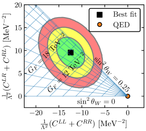
From these samples, we construct the 68, 95, and 99.7% highest-posterior-density credible intervals, which are shown in figure 2. We also compare the LEFT fit results and the predictions of QED alone to the JADE data, as shown in figure 3.

Refer to caption
Figure 2: Posterior probability density for the LEFT Wilson coefficients. The green, yellow, and red regions contain 68, 95, and 99.7% of the posterior probability, respectively. The black square shows the location of the maximum posterior probability density. The red dot shows the values of the LEFT Wilson coefficients predicted by QED alone. QED alone is very strongly disfavored.
Refer to caption
Figure 3: The JADE data (dots with error bars), compared to the prediction from QED alone (dashed line) and to the predictions resulting from the fit to the LEFT (solid line, with 68 and 95% credible intervals shown in green and yellow, respectively). The JADE data is inconsistent with QED alone, especially at higher center-of-mass energies, but it is consistent with the LEFT predictions.

The prediction of QED alone, without any electroweak contributions, predicts that the LEFT Wilson coefficients are all zero. Figure 2 shows that QED alone is very strongly disfavored. In other words, from this JADE data, we have “discovered” physics beyond QED.

This is the situation in which we hope to find ourselves when measuring SMEFT Wilson coefficients at the LHC, that we measure some Wilson coefficients and strongly disfavor the SM. The central question that is addressed by this case study is what happens next, and what this measurement can tell us about the new physics that we have observed.

5 Matching to the electroweak theory

In the event that some Wilson coefficient measurement strongly disfavors the SM, one would look for models of physics beyond the SM, and ask what Wilson coefficients those models would predict as a function of the model parameters. The effective field theory formalism allows many models to be directly compared to the data without requiring a dedicated measurement for each model.

In the case of the JADE data, the obvious model to consider is the electroweak theory Glashow:1961tr ; Weinberg:1967tq ; Salam:1968rm . At tree level, the electroweak theory adds one Feynman diagram, which contains a $\mathit{{Z}{}_{\mspace{-3.0mu}\scriptstyle{}}^{\mspace{-1.0mu}\scriptstyle{}}}$ boson in the $s$ channel, as shown in figure 4. We can calculate the differential cross section of the electroweak theory in the limit of massless fermions and a zero-width $\mathit{{Z}{}_{\mspace{-3.0mu}\scriptstyle{}}^{\mspace{-1.0mu}\scriptstyle{}}}$ boson,

$\displaystyle\begin{split}\frac{\mathrm{d}\sigma}{\mathrm{d}\cos\theta}=&\frac{\pi\alpha^{2}}{2s}\left(1+\cos^{2}\theta\right)\\ &+\frac{s}{\pi}\left(\frac{G_{F}M_{\mathit{{Z}{}_{\mspace{-3.0mu}\scriptstyle{}}^{\mspace{-1.0mu}\scriptstyle{}}}}^{2}}{s-M_{\mathit{{Z}{}_{\mspace{-3.0mu}\scriptstyle{}}^{\mspace{-1.0mu}\scriptstyle{}}}}^{2}}\right)^{2}\left[\left(g_{V}^{2}+g_{A}^{2}\right)^{2}\left(1+\cos^{2}\theta\right)+8g_{V}^{2}g_{A}^{2}\cos\theta\right]\\ &+\sqrt{2}\alpha\frac{G_{F}M_{\mathit{{Z}{}_{\mspace{-3.0mu}\scriptstyle{}}^{\mspace{-1.0mu}\scriptstyle{}}}}^{2}}{s-M_{\mathit{{Z}{}_{\mspace{-3.0mu}\scriptstyle{}}^{\mspace{-1.0mu}\scriptstyle{}}}}^{2}}\left[g_{V}^{2}\left(1+\cos^{2}\theta\right)+2g_{A}^{2}\cos\theta\right],\end{split}$ (2)

where $G_{F}$ is Fermi’s constant, $M_{\mathit{{Z}{}_{\mspace{-3.0mu}\scriptstyle{}}^{\mspace{-1.0mu}\scriptstyle{}}}}$ is the mass of the $\mathit{{Z}{}_{\mspace{-3.0mu}\scriptstyle{}}^{\mspace{-1.0mu}\scriptstyle{}}}$ boson, $g_{V}=\sin^{2}\theta_{W}-1/4$ and $g_{A}=-1/4$ are the vector and axial-vector couplings of the $\mathit{{Z}{}_{\mspace{-3.0mu}\scriptstyle{}}^{\mspace{-1.0mu}\scriptstyle{}}}$ boson to the electron and muon, and $\theta_{W}$ is the weak mixing angle. Comparing eqs. 1 and 2, or better yet comparing the LEFT and electroweak calculations at the matrix-element level, we can obtain the electroweak predictions for the LEFT Wilson coefficients,

$\displaystyle\frac{1}{\Lambda^{2}}\Re\left(C^{LL}+C^{RR}\right)$ $\displaystyle=-8\sqrt{2}G_{F}(g_{V}^{2}+g_{A}^{2})$
$\displaystyle\frac{1}{\Lambda^{2}}\Re\left(C^{LR}+C^{RL}\right)$ $\displaystyle=-8\sqrt{2}G_{F}(g_{V}^{2}-g_{A}^{2}).$
{feynman}\vertex$\mathit{{{\mathit{{e}{}_{\mspace{-3.0mu}\scriptstyle{}}^{\mspace{-1.0mu}\scriptstyle{}}}}}{}_{\mspace{-3.0mu}\scriptstyle{}}^{\mspace{-1.0mu}\scriptstyle{-}}}$\vertex$\mathit{{{\mathit{{e}{}_{\mspace{-3.0mu}\scriptstyle{}}^{\mspace{-1.0mu}\scriptstyle{}}}}}{}_{\mspace{-3.0mu}\scriptstyle{}}^{\mspace{-1.0mu}\scriptstyle{+}}}$\vertex\vertex\vertex$\mathit{{{\mathit{{\upmu}{}_{\mspace{-3.0mu}\scriptstyle{}}^{\mspace{-1.0mu}\scriptstyle{}}}}}{}_{\mspace{-3.0mu}\scriptstyle{}}^{\mspace{-1.0mu}\scriptstyle{-}}}$\vertex$\mathit{{{\mathit{{\upmu}{}_{\mspace{-3.0mu}\scriptstyle{}}^{\mspace{-1.0mu}\scriptstyle{}}}}}{}_{\mspace{-3.0mu}\scriptstyle{}}^{\mspace{-1.0mu}\scriptstyle{+}}}$\diagram$\mathit{{Z}{}_{\mspace{-3.0mu}\scriptstyle{}}^{\mspace{-1.0mu}\scriptstyle{}}}$
Figure 4: The tree-level $\mathit{{Z}{}_{\mspace{-3.0mu}\scriptstyle{}}^{\mspace{-1.0mu}\scriptstyle{}}}$ boson exchange Feynman diagram from the electroweak theory.

6 Extracting the weak boson masses

Now that we have predictions for the LEFT Wilson coefficients as functions of the parameters of the electroweak theory, we can reformulate the posterior probability density for the LEFT Wilson coefficients as a posterior probability density for the electroweak parameters $G_{F}$ and $\sin^{2}\theta_{W}$ or, equivalently, $M_{\mathit{{W}{}_{\mspace{-3.0mu}\scriptstyle{}}^{\mspace{-1.0mu}\scriptstyle{}}}}$ and $M_{\mathit{{Z}{}_{\mspace{-3.0mu}\scriptstyle{}}^{\mspace{-1.0mu}\scriptstyle{}}}}$.

In figure 5, we overlay lines of constant $G_{F}$ and lines of constant $\sin^{2}\theta_{W}$ on the posterior probability density of figure 2. As $G_{F}$ approaches 0, we recover the QED-only prediction. At $\sin^{2}\theta_{W}=0$, $C^{LR}+C^{RL}=0$, and as $\sin^{2}\theta_{W}$ approaches 0.25, we have $C^{LL}+C^{RR}=-(C^{LR}+C^{RL})$. As $\sin^{2}\theta_{W}$ continues to increase beyond 0.25, we move back downwards in figure 5, so that the line for $\sin^{2}\theta_{W}=0.5$ lies on top of the line for $\sin^{2}\theta_{W}=0$. This implies that the portion of the posterior probability density that lies above and to the right of the line for $\sin^{2}\theta_{W}=0.25$ is forbidden, and the rest of the space is double-covered.

Refer to caption
Figure 5: Posterior probability density for the LEFT Wilson coefficients, with contours of constant $G_{F}$ and contours of constant $\sin^{2}\theta_{W}$ overlaid.

When extracting the electroweak parameters, we remove the forbidden portion of the posterior probability density, and re-scale the remaining region to a total posterior probability of 1. To handle the double cover, we exploit our knowledge that $\sin^{2}\theta_{W}$ is less than 0.25, and so restrict ourselves to only considering that portion of the electroweak parameter space.

With this understanding, along with the relationship between $M_{\mathit{{W}{}_{\mspace{-3.0mu}\scriptstyle{}}^{\mspace{-1.0mu}\scriptstyle{}}}}$, $M_{\mathit{{Z}{}_{\mspace{-3.0mu}\scriptstyle{}}^{\mspace{-1.0mu}\scriptstyle{}}}}$ and $G_{F}$, $\sin^{2}\theta_{W}$,

$\displaystyle M_{\mathit{{W}{}_{\mspace{-3.0mu}\scriptstyle{}}^{\mspace{-1.0mu}\scriptstyle{}}}}^{2}$ $\displaystyle=\frac{\pi\alpha}{\sqrt{2}G_{F}\sin^{2}\theta_{W}}$
$\displaystyle M_{\mathit{{Z}{}_{\mspace{-3.0mu}\scriptstyle{}}^{\mspace{-1.0mu}\scriptstyle{}}}}^{2}$ $\displaystyle=\frac{\pi\alpha}{\sqrt{2}G_{F}\left(1-\sin^{2}\theta_{W}\right)\sin^{2}\theta_{W}},$

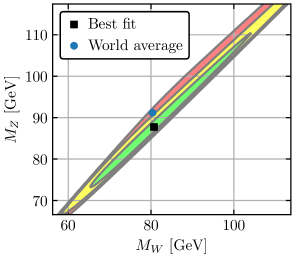
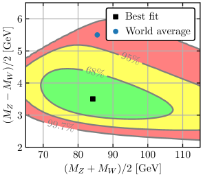
we extract the posterior probability density for $M_{\mathit{{W}{}_{\mspace{-3.0mu}\scriptstyle{}}^{\mspace{-1.0mu}\scriptstyle{}}}}$ and $M_{\mathit{{Z}{}_{\mspace{-3.0mu}\scriptstyle{}}^{\mspace{-1.0mu}\scriptstyle{}}}}$, which is shown in figure 6 along with the posterior probability density for $(M_{\mathit{{W}{}_{\mspace{-3.0mu}\scriptstyle{}}^{\mspace{-1.0mu}\scriptstyle{}}}}-M_{\mathit{{Z}{}_{\mspace{-3.0mu}\scriptstyle{}}^{\mspace{-1.0mu}\scriptstyle{}}}})/2$ and $(M_{\mathit{{W}{}_{\mspace{-3.0mu}\scriptstyle{}}^{\mspace{-1.0mu}\scriptstyle{}}}}+M_{\mathit{{Z}{}_{\mspace{-3.0mu}\scriptstyle{}}^{\mspace{-1.0mu}\scriptstyle{}}}})/2$. The JADE data, considered through the lens of the LEFT, provides a measurement of the $\mathit{{W}{}_{\mspace{-3.0mu}\scriptstyle{}}^{\mspace{-1.0mu}\scriptstyle{}}}$ and $\mathit{{Z}{}_{\mspace{-3.0mu}\scriptstyle{}}^{\mspace{-1.0mu}\scriptstyle{}}}$ boson masses that is remarkably accurate, albeit with large uncertainties. The average of the $\mathit{{W}{}_{\mspace{-3.0mu}\scriptstyle{}}^{\mspace{-1.0mu}\scriptstyle{}}}$ and $\mathit{{Z}{}_{\mspace{-3.0mu}\scriptstyle{}}^{\mspace{-1.0mu}\scriptstyle{}}}$ boson masses is extremely close to the world average although their difference disagrees with the world average at a level of more than 2 standard deviations.

Refer to caption
Refer to caption
Figure 6: The measured masses of the $\mathit{{W}{}_{\mspace{-3.0mu}\scriptstyle{}}^{\mspace{-1.0mu}\scriptstyle{}}}$ and $\mathit{{Z}{}_{\mspace{-3.0mu}\scriptstyle{}}^{\mspace{-1.0mu}\scriptstyle{}}}$ bosons along with 68, 95, and 99.7% credible regions, shown in green, yellow, and red, respectively. The black square shows the maximum posterior density, and the blue dot shows the current world average. The left plot shows the $\mathit{{W}{}_{\mspace{-3.0mu}\scriptstyle{}}^{\mspace{-1.0mu}\scriptstyle{}}}$ and $\mathit{{Z}{}_{\mspace{-3.0mu}\scriptstyle{}}^{\mspace{-1.0mu}\scriptstyle{}}}$ boson masses, while the right plot shows the average of the $\mathit{{W}{}_{\mspace{-3.0mu}\scriptstyle{}}^{\mspace{-1.0mu}\scriptstyle{}}}$ and $\mathit{{Z}{}_{\mspace{-3.0mu}\scriptstyle{}}^{\mspace{-1.0mu}\scriptstyle{}}}$ boson masses and half the difference between their masses. This measurement disagrees with the world average at a level of more than 2 standard deviations.

There are many possible reasons for this discrepancy, including but not limited to neglected higher order corrections in the QED, electroweak, and LEFT calculations, neglected renormalization group running of the fine-structure constant, neglected correlations in the uncertainties in the JADE data, and neglected higher-dimension LEFT operators. Given these known deficiencies, it is remarkable how well we are able to determine the masses of the weak bosons from only this one data set seen through the lens of effective field theory.

This measurement of the $\mathit{{W}{}_{\mspace{-3.0mu}\scriptstyle{}}^{\mspace{-1.0mu}\scriptstyle{}}}$ and $\mathit{{Z}{}_{\mspace{-3.0mu}\scriptstyle{}}^{\mspace{-1.0mu}\scriptstyle{}}}$ boson masses would have been sufficient to guide the construction of then-future colliders such as the super proton-antiproton synchrotron, which discovered the $\mathit{{W}{}_{\mspace{-3.0mu}\scriptstyle{}}^{\mspace{-1.0mu}\scriptstyle{}}}$ and $\mathit{{Z}{}_{\mspace{-3.0mu}\scriptstyle{}}^{\mspace{-1.0mu}\scriptstyle{}}}$ bosons UA1:1983crd ; UA1:1983mne ; UA2:1983mlz ; UA2:1983tsx , and the large electron-positron collider, which measured the properties of the $\mathit{{Z}{}_{\mspace{-3.0mu}\scriptstyle{}}^{\mspace{-1.0mu}\scriptstyle{}}}$ boson in unsurpassed detail ALEPH:2005ab . Accordingly, we anticipate that, given an observation of SMEFT Wilson coefficients in significant tension with the SM at the LHC, matching to UV-complete models will permit sufficient understanding of the parameters of those models to guide the construction of future colliders such as ILC, CLiC, FCC-ee, FCC-hh, CEPC, or a muon collider.

7 Conclusion

The low-energy effective field theory provides an adequate description of the JADE ${\mathit{{{\mathit{{e}{}_{\mspace{-3.0mu}\scriptstyle{}}^{\mspace{-1.0mu}\scriptstyle{}}}}}{}_{\mspace{-3.0mu}\scriptstyle{}}^{\mspace{-1.0mu}\scriptstyle{+}}}}{\mathit{{{\mathit{{e}{}_{\mspace{-3.0mu}\scriptstyle{}}^{\mspace{-1.0mu}\scriptstyle{}}}}}{}_{\mspace{-3.0mu}\scriptstyle{}}^{\mspace{-1.0mu}\scriptstyle{-}}}}\to{\mathit{{{\mathit{{\upmu}{}_{\mspace{-3.0mu}\scriptstyle{}}^{\mspace{-1.0mu}\scriptstyle{}}}}}{}_{\mspace{-3.0mu}\scriptstyle{}}^{\mspace{-1.0mu}\scriptstyle{+}}}}{\mathit{{{\mathit{{\upmu}{}_{\mspace{-3.0mu}\scriptstyle{}}^{\mspace{-1.0mu}\scriptstyle{}}}}}{}_{\mspace{-3.0mu}\scriptstyle{}}^{\mspace{-1.0mu}\scriptstyle{-}}}}$ data below the $\mathit{{Z}{}_{\mspace{-3.0mu}\scriptstyle{}}^{\mspace{-1.0mu}\scriptstyle{}}}$ boson mass. It permits the observation of physics beyond QED with a high level of significance, more than 5 standard deviations. Furthermore, by matching the measured Wilson coefficients of the low-energy effective field theory to the electroweak theory, we can obtain a rough measurement of the masses of the $\mathit{{W}{}_{\mspace{-3.0mu}\scriptstyle{}}^{\mspace{-1.0mu}\scriptstyle{}}}$ and $\mathit{{Z}{}_{\mspace{-3.0mu}\scriptstyle{}}^{\mspace{-1.0mu}\scriptstyle{}}}$ bosons. This measurement would have been sufficient, even in the absence of other data, to guide the construction of the super proton-antiproton synchrotron and the large electron-positron collider.

Accordingly, as we search for signs of physics beyond the standard model using the standard model effective field theory, we anticipate that a discovery will provide sufficient information, by matching to one or more UV-complete models, to guide the construction of future colliders such as ILC, CLiC, FCC-ee, FCC-hh, CEPC, or a muon collider. This case study demonstrates both the limitations and the power of effective field theory as a tool to discover and characterize new physics, and provides hope and guidance to the effective field theory efforts at the LHC and beyond.

Acknowledgements.
We would like to thank Jennet Dickinson and Michael Peskin for helpful discussions and suggestions. This work was supported by DOE grant DE-SC0007861.

References

  • (1) SMEFiT collaboration, Combined SMEFT interpretation of Higgs, diboson, and top quark data from the LHC, JHEP 11 (2021) 089 [2105.00006].
  • (2) B. Naroska, e+e- physics with the jade detector at petra, Physics Reports 148 (1987) 67.
  • (3) JADE collaboration, New Results on $e^{+}e^{-}\to\mu^{+}\mu^{-}$ From the Jade Detector at PETRA, Z. Phys. C 26 (1985) 507.
  • (4) E.E. Jenkins, A.V. Manohar and P. Stoffer, Low-Energy Effective Field Theory below the Electroweak Scale: Operators and Matching, JHEP 03 (2018) 016 [1709.04486].
  • (5) T. Wiecki, R. Vieira, J. Salvatier, M. Kochurov, A. Patil, M. Osthege et al., pymc-devs/pymc: v5.16.1, June, 2024. 10.5281/zenodo.12544153.
  • (6) S.L. Glashow, Partial Symmetries of Weak Interactions, Nucl. Phys. 22 (1961) 579.
  • (7) S. Weinberg, A Model of Leptons, Phys. Rev. Lett. 19 (1967) 1264.
  • (8) A. Salam, Weak and Electromagnetic Interactions, Conf. Proc. C 680519 (1968) 367.
  • (9) UA1 collaboration, Experimental Observation of Isolated Large Transverse Energy Electrons with Associated Missing Energy at $\sqrt{s}=540$ GeV, Phys. Lett. B 122 (1983) 103.
  • (10) UA1 collaboration, Experimental Observation of Lepton Pairs of Invariant Mass Around 95-GeV/c**2 at the CERN SPS Collider, Phys. Lett. B 126 (1983) 398.
  • (11) UA2 collaboration, Evidence for $Z^{0}\to e^{+}e^{-}$ at the CERN $\bar{p}p$ Collider, Phys. Lett. B 129 (1983) 130.
  • (12) UA2 collaboration, Observation of Single Isolated Electrons of High Transverse Momentum in Events with Missing Transverse Energy at the CERN anti-p p Collider, Phys. Lett. B 122 (1983) 476.
  • (13) ALEPH, DELPHI, L3, OPAL, SLD, LEP Electroweak Working Group, SLD Electroweak Group, SLD Heavy Flavour Group collaboration, Precision electroweak measurements on the $Z$ resonance, Phys. Rept. 427 (2006) 257 [hep-ex/0509008].