Dark energy evolution from quantum gravity

Abstract

If an ultraviolet fixed point renders quantum gravity renormalizable, the effective potential for a singlet scalar field – the cosmon – can be computed according to the corresponding scaling solution of the renormalization group equations. We associate the largest intrinsic mass scale generated by the flow away from the fixed point with the scale of present dark energy density. This results in a highly predictive scenario for the evolution of dynamical dark energy. It solves the cosmological constant problem dynamically, and may be called ”quantum gravity quintessence”. A first setting without quantum scale symmetry violation in the neutrino sector could explain the present amount of dark energy, but fails for the constraints on its time evolution. In contrast, a logarithmic scale symmetry violation in the beyond standard model sector responsible for the neutrino masses induces a non-vanishing cosmon-neutrino coupling in the Einstein frame. This yields a cosmology similar to growing neutrino quintessence, which could be compatible with present observation. The small number of unknown parameters turns the scaling solution for quantum gravity into a fundamental explanation of dynamical dark energy which can be falsified.

Already in the first paper on dynamical dark energy or quintessence [1] quantum scale symmetry [2] has played a central role. In quantum gravity the fate of quantum scale symmetry is closely related to the presence of an ultraviolet fixed point of the renormalization group equation, which may be asymptotically safe [3, 4] or asymptotically free [5, 6, 7, 8]. For a world living exactly on the fixed point quantum scale symmetry is typically an exact symmetry. In contrast, for a crossover between two fixed points, or in case of a flow away from the ultraviolet fixed point due to a relevant parameter, an intrinsic mass scale yields an explicit breaking of quantum scale symmetry or dilatation symmetry. This intrinsic mass scale can be viewed as dimensional transmutation of running couplings, somewhat similar to the confinement scale in quantum chromodynamics. The largest intrinsic mass scale sets the overall scale of the model and has no directly observable meaning. Only dimensionless ratios, as particle masses or field values in units of this mass scale, are observable. In quantum gravity the largest intrinsic mass scale is often associated with the Planck mass. There is no need for this, however, since a dynamical Planck mass may be given by the value of a scalar field rather than being an intrinsic scale. We propose to associate the largest intrinsic mass scale with a much smaller scale, typically of the order of a few meV – a scale characteristic for the masses of neutrinos and the present dark energy density. This simple assumption leads to a highly predictive setting for dynamical dark energy [9, 10] that we call ”quantum gravity quintessence”.

The basic reason for predictivity is the observation that for momentum scales or field values much larger than the intrinsic scale the latter becomes negligible. In this case all properties can be computed from the scaling solution of the renormalization flow. Scaling solutions are particular solutions of systems of non-linear differential equations. Their existence imposes severe constraints which encode properties that may not be recognized by too simple ”naturalness arguments” for the role of quantum fluctuations. The renormalization group equations or flow equations deal already with the quantum effective action which includes all effects of quantum fluctuations. The flow equations, and therefore their particular scaling solutions, are due to quantum effects.

In functional renormalization the dimensionless couplings are not only functions of a renormalization scale $k$. They are also functions of the cosmon field $\chi$. For example, the dimensionless effective potential of the cosmon $u=V(\chi,k)/k^{4}$ depends, in general, both on $k$ and on $\chi$. For a scaling solution $u$ is only a function of the dimensionless ratio $\chi/k$. Once this function is computed, all cosmon self-interactions, quartic, sextic and so on, are given. Similarly, the coefficient of the curvature scalar $F$ (effective squared Planck mass) defines a dimensionless ratio $f=F/k^{2}$. For the scaling solution $f$ is only a function of $\chi/k$. The same holds for the coefficient of the kinetic term of the cosmon $K$. If $u$, $f$ and $K$ can be computed, the cosmological field equations derived by variation of this quantum effective action lead to typical models of ”variable gravity” [11].

Already the first computations of models of a singlet scalar field coupled to the metric (”dilaton quantum gravity”) have revealed a simple behavior for large $\chi/k$ [12, 13]. The function $f$ increases quadratically with $\chi$, $f\sim\chi^{2}/k^{2}$, such that $F=\xi\chi^{2}$. The dimensionless coupling $\xi$ is the non-minimal coupling of the scalar field to gravity. It is found not to vanish. On the other hand, for the scaling solution the potential settles to a constant for large $\chi$, $u(\chi/k)\to u_{\infty}$, $V=u_{\infty}k^{4}$. The scaling solution describes a crossover from an ultraviolet fixed point for $\chi/k\to 0$ to an infrared fixed point for $\chi/k\to\infty$. For a scaling solution describing a crossover the intrinsic scale is set by $k$. The intrinsic scale has a dominant effect for the scalar potential $V\sim k^{4}$, while for the coefficient of the curvature scalar it remains subdominant, $F\sim\xi\chi^{2}+f_{\infty}k^{2}$.

The present cosmological epoch is very close to the infrared fixed point, since the ratio $\chi/k$ has grown to huge values $\sim 10^{30}$ during the long history of the universe. This has crucial consequences for predictivity. First, the effects of the metric fluctuations are tiny, being suppressed by powers of $k^{2}/\chi^{2}$. (An exception is the contribution to a constant term in the scalar effective potential.) Second, for momenta or field values much larger than the neutrino mass the intrinsic scale $k$ becomes negligible. In this momentum range one obtains the scale invariant standard model [1, 14, 15], with all mass scales (e.g. Fermi scale, confinement scale) proportional to $\chi$. This proportionality is a simple consequence of quantum scale symmetry which becomes exact for $k\to 0$. The particles and couplings of the standard model are well known, such that the renormalization group equations can be computed without additional unknown parameters. The functional flow equations coincide with the ones from perturbation theory.

A loophole for predictivity arises from possible beyond standard model (BSM) physics. Even though the BSM sector may not involve additional light particles, it manifests itself through the masses of neutrinos. They are due to dimension five operators which involve a heavy scale where the symmetry B-L is spontaneously broken. We explore here two cases. For the first, the neutrino masses are exactly proportional to $\chi$. In this case the model is very predictive for cosmology. The field equations for the cosmon admit solutions for which the present amount of dark energy can be obtained. This is already rather remarkable since no small dimensionless parameter is present, and the tiny ratio $V/F^{2}\sim 10^{-120}$ arises from the dynamical increase of $\chi/k$ over the history of the universe. The detailed equation of state is not compatible with observation, however.

For our second case we consider the possibility that quantum scale symmetry violation in the BSM-sector induces an additional dependence of neutrino masses on $\chi/k$. This dependence will become computable only once a given BSM-sector is assumed. At the present stage, we parameterize the logarithmic running in the BSM-sector by a single free parameter, such that the model still remains highly predictive. The outcome is a model close to growing neutrino quintessence [16, 17] which may well be compatible with present observation.

Cosmon potential from quantum gravity

Quantum gravity computations of the flowing effective action by use of functional flow equations typically yield for a range of fields relevant for our purpose the quantum effective action according to the scaling solution,

$$\Gamma_{k}=\int_{x}\sqrt{g^{\prime}}\left\{-\frac{\xi}{2}\chi^{2}R^{\prime}+u(\chi)k^{4}+\frac{1}{2}K(\chi)\partial^{\mu}\chi\partial_{\mu}\chi\right\}\ .$$ (1)

The central point for predictivity is the computation of $u(\chi)$ according to the scaling solution of quantum gravity. For $K(\chi)/\xi$ computations with a similar reliability are not available at the present stage.

For the computation of observational consequences it is most suitable to work in the Einstein frame with a fixed (reduced) Planck mass $M=2.436\cdot 10^{18}\,\text{GeV}$. The field equations follow then from a quantum effective action

$$\Gamma=\int_{x}\sqrt{g}\left\{-\frac{M^{2}}{2}R+U_{E}(\varphi)+\frac{1}{2}Z\partial^{\mu}\varphi\partial_{\mu}\varphi\right\}\ .$$ (2)

Here the “wave function renormalization” or “kinetial” $Z$ is, in general, a function of $\varphi$. The Weyl transformation to the Einstein frame results in

$$U_{E}(\varphi)=\frac{u(\chi)k^{4}M^{4}}{\xi^{2}\chi^{4}}\ ,$$ (3)

with scalar field $\chi$ and $\varphi$ related by

$$\varphi=4M\ln\left(\frac{\chi}{k}\right)\ .$$ (4)

For constant $\xi$ one has

$$Z(\varphi)=\frac{1}{16}\left(\frac{K(\chi)}{\xi}+6\right)\ .$$ (5)

Given the lack of a reliable quantum gravity computation at the present stage we take here a constant $Z$ as one of the parameters of our model.

If $u(\chi)$ reaches for asymptotically large $\chi$ a constant $u_{\infty}$ and $\xi$ is constant, the potential $U_{E}(\varphi)$ decreases exponentially,

$$U_{E}=\frac{u_{\infty}M^{4}}{\xi^{2}}\exp\left(-\frac{\varphi}{M}\right)\ .$$ (6)

This amounts to a possible dynamical solution of the cosmological constant problem [1] for cosmologies where $\varphi$ diverges in the infinite future. At present, $\varphi/M$ is large but finite, resulting in very small $U_{E}$ as needed for an explanation of the present value of the dark energy density.

The functional flow equation for the dimensionless potential $u=V(\chi)/k^{4}$ describes its dependence on the renormalization scale $k$, which is given by an infrared cutoff such that in a Euclidean setting only fluctuations with squared momentum $q^{2}$ larger than $k^{2}$ are included,

$$k\partial_{k}u=-4u+2\tilde{\rho}\partial_{\tilde{\rho}}u+4c_{U}\ .$$ (7)

This flow equation holds at fixed $\tilde{\rho}=\chi^{2}/(2k^{2})$. The term $-4u$ reflects the denominator in the ratio $u=V/k^{4}$, the term $-2\tilde{\rho}\partial_{\tilde{\rho}}$ results from the transition of the flow at fixed $\chi$ to fixed $\tilde{\rho}$, and the last term $c_{U}$ describes the effect of fluctuations on the $k$-dependence of $V(\chi)$. One finds [18, 19]

$$c_{U}=\frac{1}{128\pi^{2}}\big{(}\bar{N}_{S}(\tilde{\rho})+2\bar{N}_{V}(\tilde{\rho})-2\bar{N}_{F}(\tilde{\rho})+\bar{N}_{g}(\tilde{\rho})\big{)}\ ,$$ (8)

with $\bar{N}_{S}$, $\bar{N}_{V}$, and $\bar{N}_{F}$ the effective numbers of scalars, gauge bosons and Weyl-fermions, which depend on $\tilde{\rho}$ through $\tilde{\rho}$-dependent particle masses. (For computations of the flow of the scalar potential within various approximations and truncations see refs. [20, 21, 22, 23, 24, 25, 26].) The contributions from non-gravitational fluctuations (matter fluctuations) are the standard result for functional flow equations [27, 28], which are well tested in a large variety of applications [29]. They include one-loop perturbation theory. In a version of gauge invariant flow equations [30] the contribution from metric fluctuations can be approximated [31] by

$$\bar{N}_{g}=\frac{5}{1-v}+\frac{1}{1-v/4}-4\ ,\quad v=\frac{u}{\xi\tilde{\rho}}\ .$$ (9)

For the large values of $\tilde{\rho}$ relevant here $v$ is tiny, resulting in constant $\bar{N}_{g}=2$, corresponding to the two massless graviton degrees of freedom.

In the flow equation (8) the contributions of bosons are positive, while the contributions of fermions are negative. This reflects the well known signs of the fluctuation contributions to the cosmological constant – the scalar potential can be seen as a field-dependent cosmological constant. These different signs will play an important role for the present note since they are responsible for a negative potential $U_{E}(\varphi)$ in a certain range of $\varphi$.

The effective particle numbers $\bar{N}$ involve threshold functions which account for the decoupling of heavy particles once their squared mass $m^{2}$ is larger than the cutoff $k^{2}$. Details of the threshold functions depend on the precise form of the cutoff. For the Litim cutoff [32] or the simplified flow equation [33] one has for the fermions

$$\bar{N}_{F}=\sum_{f}\big{(}1+\tilde{m}_{f}^{2}\big{)}^{-1}\ ,\quad\tilde{m}_{f}^{2}=\frac{m_{f}^{2}(\tilde{\rho})}{k^{2}}\ .$$ (10)

Here the sum over $f$ runs over all Weyl- (or equivalently Majorana-) fermions with mass $m_{f}$. The fermion masses depend on the scalar field $\chi$ and we write

$$m_{f}=h_{f}\chi\ ,\quad\tilde{m}_{f}^{2}(\tilde{\rho})=2h_{f}^{2}(\tilde{\rho})\tilde{\rho}\ ,$$ (11)

with the effective Yukawa couplings $h_{f}$. Exact quantum scale symmetry implies constant $h_{f}$. For example, the effective Yukawa coupling $h_{e}$ for the electron is of the form $h_{e}=y_{e}\varphi_{0}(\chi)/\chi$, with vacuum expectation value of the Higgs doublet $\varphi_{0}(\chi)$ proportional to $\chi$ and $y_{e}$ the Yukawa coupling to the Higgs doublet. The electroweak gauge hierarchy requires a tiny value of $\varphi_{0}/\chi$, implying a very small effective Yukawa coupling $h_{e}$. From the measured ratio of electron mass $m_{e}$ to Planck mass $M$ one infers

$$h_{e}=\frac{\sqrt{\xi}m_{e}}{M}\ .$$ (12)

In order to compute the relevant value of $\tilde{m}^{2}$ for a given stage of the cosmological evolution we need the relevant value of $\tilde{\rho}$. The units of $k$ are arbitrary. We choose units which identify the present value of the potential with the present observed dark energy density, which obtains for a present Hubble parameter $h=0.7$ and dark energy fraction $\Omega_{h,0}=0.7$ as

$$u(t_{0})k^{4}=U_{E}(t_{0})=(2.229\cdot 10^{-3}\,\text{eV})^{4}\ .$$ (13)

For realistic cosmology with $U_{E}(t_{0})/M^{4}\approx 10^{-120}$ the present value of $\chi/k$ must be very large according to $M^{2}=\xi\chi^{2}(t_{0})$,

$$U_{E}(t_{0})=\frac{u(t_{0})M^{4}}{\xi^{2}}\exp\left(-\frac{\varphi(t_{0})}{M}\right)=\frac{u(t_{0})M^{4}}{4\xi^{2}}\tilde{\rho}(t_{0})^{-2}\ .$$ (14)

With $u(t_{0})$ a few times $(128\pi^{2})^{-1}$, see below, this amounts to a very large present value of $\tilde{\rho}$ somewhere around $\tilde{\rho}(t_{0})\approx 10^{58}$. This large value will be related later to the increase of $\tilde{\rho}(t)$ over a huge time period in Planck units – it is a consequence of the huge age of our universe.

We may evaluate the present value of the dimensionless neutrino mass $\tilde{m}_{\nu}$,

$$\tilde{m}_{\nu}^{2}(t_{0})=\sqrt{u(t_{0})}\left(\frac{m_{\nu}}{2.229\cdot 10^{-3}\,\text{eV}}\right)^{2}\ .$$ (15)

This leads to the interesting conclusion that the present epoch of cosmology coincides roughly with the epoch when the neutrino fluctuations decouple from the flow of the effective potential. It may therefore not be surprising that close to the present epoch important qualitative changes can occur in the evolution of dynamical dark energy. On the other hand, in the present epoch electrons and all other charged fermions have already decoupled from the flow.

For the boson fluctuations only the photon, the cosmon and the graviton contribute to the flow of the potential in the range of $\tilde{\rho}$ relevant for the present cosmological epoch. Photons are massless, resulting in $\bar{N}_{V}=1$. For the cosmon fluctuations the mass term is given by the second derivative of the effective potential with respect to $\chi$,

$$\bar{N}_{S}=\frac{1}{1+u^{\prime}+2\tilde{\rho}u^{\prime\prime}}\ ,$$ (16)

where primes denote derivatives with respect to $\tilde{\rho}$, $u^{\prime}=\partial_{\tilde{\rho}}u$. This completes the flow generator $c_{U}$ for the range of $\tilde{\rho}$ relevant for cosmology close to the present epoch. For earlier epochs $\tilde{\rho}(t)$ is smaller than $\tilde{\rho}(t_{0})$. Electron fluctuations matter for a range of $\tilde{\rho}$ smaller than $h_{e}^{-2}$. For even much smaller $\tilde{\rho}$ one has to include fluctuation contributions from muons and pions, and so on.

The differential equation (7) admits a scaling solution for $k\partial_{k}u=0$. It is given by a solution of the non-linear differential equation

$$\tilde{\rho}\partial_{\tilde{\rho}}u=2(u-c_{U})\ .$$ (17)

The solution of this non-linear differential equation has to exist for the whole range $0\leq\tilde{\rho}<\infty$. Combined with a similar equation for $f(\tilde{\rho})$ this imposes severe constraints, such that the only scaling solutions found have constant $u$ for $\tilde{\rho}\to\infty$. With boundary condition $u(\tilde{\rho}\to\infty)=u_{\infty}$ the scaling solution reads [10]

$$u=\frac{5}{128\pi^{2}}-\frac{1}{64\pi^{2}}\sum_{f}t_{u}\big{(}\tilde{m}_{f}^{2}\big{)}\ ,$$ (18)

with integrated threshold function,

$$t_{u}(x)=1-2x-2x^{2}\ln\left(\frac{x}{1+x}\right)\ ,$$ (19)

describing the decoupling for large $x$, i.e. $t_{u}(x\gg 1)=2/(3x)$. In the range of $\tilde{\rho}$ relevant for present cosmology only the neutrinos contribute effectively in the sum over fermions. For the cosmon contribution we employ

$$u^{\prime} =-\frac{1}{64\pi^{2}}\sum_{f}\partial_{\tilde{\rho}}t_{u}\big{(}\tilde{m}_{f}^{2}\big{)}$$ (20)

$$=\frac{1}{32\pi^{2}}\sum_{f}\left(\frac{1}{\tilde{\rho}}+\partial_{\tilde{\rho}}\ln h_{f}^{2}\right)\left(\frac{1}{1+\tilde{m}_{f}^{2}}-t_{u}\big{(}\tilde{m}_{f}^{2}\big{)}\right)\ ,$$

and infer that the scalar mass is tiny in the relevant range of $\tilde{\rho}$, $\bar{N}_{S}=1$. The factor $5$ in eq. (18) simply counts the number of massless bosonic degrees of freedom. (We have neglected in the flow equation mixing effects between metric- and scalar fluctuations [34]. They do not alter the conclusion $\bar{N}_{g}+\bar{N}_{S}=3$ for the relevant range of large $\tilde{\rho}$. The scaling solution for $u$ should be seen together with a scaling solution for the dimensionless coefficient of the curvature scalar $f$. The solution $f=2\xi\tilde{\rho}$ for large $\tilde{\rho}$ is already incorporated in our ansatz (1). In particular, there is no combined scaling solution for $u$ and $f$ which is compatible with $u(\tilde{\rho}\to\infty)\sim\tilde{\rho}^{2}$.)

The scaling solution (18) can be translated to the potential in the Einstein frame (3)

$$U_{E}=\frac{u(\varphi)M^{4}}{\xi^{2}}\exp\left(-\frac{\varphi}{M}\right)=U_{0}\frac{u(\varphi)}{u_{\infty}}\exp\left(-\frac{\varphi-\bar{\varphi}}{M}\right)\ ,$$ (21)

with $u_{\infty}=5/(128\pi^{2})\approx 0.004$. Here $U_{0}$ is a free constant that specifies the definition of $\bar{\varphi}$ and will be chosen as $U_{0}=(2.229\cdot 10^{-3}\,\text{eV})^{4}$. The constant $\bar{\varphi}$ accounts for the dominant part of $\varphi(t_{0})$ and absorbs $\xi$,

$$\frac{\bar{\varphi}}{M}=\ln\left(\frac{u_{\infty}M^{4}}{\xi^{2}U_{0}}\right)\ .$$ (22)

The present value $\varphi(t_{0})$ is given by

$$\frac{\varphi(t_{0})-\bar{\varphi}}{M}=\ln\left(\frac{u\big{(}\varphi(t_{0})\big{)}}{u_{\infty}}\right)-\ln\left(\frac{U_{E}(t_{0})}{U_{0}}\right)\ ,$$ (23)

where a realistic cosmology requires $0<u\big{(}\varphi(t_{0})\big{)}<u_{\infty}$. For $U_{E}(t_{0})=U_{0}$ this implies $\varphi(t_{0})<\bar{\varphi}$.

Besides the overall exponential factor the $\varphi$-dependence of $U_{E}(\varphi)$ is governed by

$$\frac{u(\varphi)}{u_{\infty}}=1-\frac{2}{5}\sum_{f}t_{u}\big{(}\tilde{m}_{f}^{2}(\varphi)\big{)}\ ,$$ (24)

with ($2\tilde{\rho}=\exp(\varphi/2M)$)

$$\tilde{m}_{f}^{2}(\varphi)=h_{f}^{2}(\varphi)\exp\left(\frac{\varphi}{2M}\right)=c_{f}(\varphi)\exp\left(\frac{\varphi-\bar{\varphi}}{2M}\right)\ .$$ (25)

The function

$$c_{f}(\varphi)=\frac{h_{f}^{2}(\varphi)}{h_{f}^{2}\big{(}\varphi(t_{0})\big{)}}\frac{m_{f}^{2}(t_{0})\sqrt{u_{\infty}}}{\sqrt{U_{0}}}\ ,$$ (26)

becomes a constant if the Yukawa coupling $h_{f}$ does not depend on $\tilde{\rho}$,

$$c_{f,0}=\left(\frac{m_{f}(t_{0})}{9\cdot 10^{-3}\,\text{eV}}\right)^{2}\ .$$ (27)

We first concentrate on the case of constant $h_{f}$ and discuss a possible $\varphi$-dependence in the second part.

As $\varphi$ decreases the fermion masses get smaller. For small enough $\varphi$ this leads to a negative value of $u(\varphi)$, and therefore to a negative potential $U_{E}(\varphi)$. This negative region sets in once the largest neutrino mass term $\tilde{m}_{\nu}^{2}(\varphi)$ is small enough. For the range of $\varphi$ for which $\tilde{m}_{e}^{2}\gg 1$, $\tilde{m}_{\nu}^{2}\ll 1$ one has $\bar{N}_{f}=3$ and therefore $u(\varphi)=-1/(128\pi^{2})$. The value of $\hat{\varphi}$ where the potential switches from negative to positive values depends on the generation structure of the neutrino masses. For degenerate neutrino masses it is given by $t_{u}\big{(}\tilde{m}_{\nu}^{2}(\hat{\varphi})\big{)}=5/6$ or $\tilde{m}_{\nu}^{2}\approx 1/12$. For hierarchical neutrino masses, $\tilde{m}_{1}^{2}~{},\tilde{m}_{2}^{2}\ll\tilde{m}_{3}^{2}$, $m_{3}=0.06\,\text{eV}$, the switch of sign occurs for $t_{u}\big{(}\tilde{m}_{3}^{2}\big{)}=1/2$. For hierarchical neutrino masses we plot the potential $U_{E}(\varphi)$ for the scaling solution and constant Yukawa couplings in fig. 1.

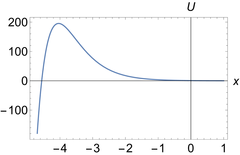
Fig. 1: Cosmon potential in the Einstein frame for the scaling solution with hierarchical neutrino masses. We plot $U_{E}/U_{0}$ as a function of $x=(\varphi-\bar{\varphi})/(2M)$.

Units of $U_{E}$ are given by $U_{0}$, and $x=(\varphi-\bar{\varphi})/(2M)=\ln\tilde{\rho}-c_{\rho}$. The maximum of the potential occurs for values rather close to the present dark energy density. For degenerate neutrino masses the potential maximum occurs for smaller $x$ and is higher.

For a given set of neutrino masses the potential $U_{E}$ for the scaling solution with constant Yukawa couplings is a parameter free function of the field variable $(\varphi-\bar{\varphi})/M$. It only depends on the masses of neutrinos. In addition, the dynamics depends on the kinetial $Z$. (We could use a canonical scalar field $\sigma$. This would lead to a one-parameter family of potentials $V(\sigma)=U_{E}\big{(}\varphi(\sigma)\big{)}$, with $\varphi-\bar{\varphi}=\sigma/\sqrt{Z}$.) In the Einstein frame the fermion masses are constant in case of field-independent Yukawa couplings.

Early cosmology for the scaling potential

For constant particle masses the evolution of the energy density of particles (radiation plus matter) follows the standard conservation laws. For a homogeneous isotropic universe the cosmological field equations read, with $t$ cosmic time, $a(t)$ the scale factor and $H(t)=\partial_{t}\ln a$ the Hubble parameter,

$$(\partial_{t}^{2}+3H\partial_{t})\varphi =-\frac{1}{Z}\frac{\partial U_{E}}{\partial\varphi}\ ,$$

$$\partial_{t}\rho_{E} =-nH\rho_{E}\ ,$$ (28)

with

$$H^{2}=\frac{1}{3M^{2}}\left[U_{E}+\frac{Z}{2}(\partial_{t}\varphi)^{2}+\rho_{E}\right]\ ,$$ (29)

and $\rho_{E}$ the energy density of matter and radiation in the Einstein frame (without the contribution of the cosmon). One has $n=4$ for radiation domination, $n=3$ for matter domination, and more generally $n$ is a smooth function of particle masses and temperature interpolating between the limits.

We are interested in solutions of these field equations for a recent cosmological epoch for which $\rho_{E}$ is dominated by non-relativistic matter, $n=3$. For this purpose we need for some suitable time $t_{\text{in}}$ the initial values $\varphi(t_{\text{in}})$, $\partial_{t}\varphi(t_{\text{in}})$ and $\rho_{E}(t_{\text{in}})$. We choose $\varphi(t_{\text{in}})$ in a range where neutrinos are the only fermions contributing to the flow equation for the cosmon potential. For establishing a range of reasonable values for $\varphi(t_{\text{in}})$ and $\partial_{t}\varphi(t_{\text{in}})$ we need to understand the qualitative features of the cosmological evolution of the scalar field prior to $t_{\text{in}}$. For realistic cosmologies the contributions of the scalar potential and kinetic energies will be very small at $t_{\text{in}}$, such that the dominant cosmology near $t_{\text{in}}$ is matter dominated with $\rho_{E}(t_{\text{in}})=3M^{2}$ $H^{2}(t_{\text{in}})=4M^{2}/(3t_{\text{in}}^{2})$.

The outcome of the investigation of early cosmology is rather simple. It establishes that for a suitable range of $Z$ the initial value $\varphi(t_{\text{in}})$ is large enough such that $x$ is on the right of the maximum in fig. 1. This amounts to a type of ”thawing dark energy” [1, 35] for which $\varphi$ remains constant for a long period in the radiation and matter dominated epochs. The gradient of the potential induces a change of $\varphi$ only recently. We next present some details leading to this conclusion.

While we focus in this note on late cosmology, our model actually covers the whole history of the universe. For small $\tilde{\rho}$ the scaling solution for $u$ may involve particles beyond the standard model, as for grand unified theories. The overall features are rather independent of the precise particle content. An early inflationary epoch requires positive $U_{E}$ for a range of small $\chi$. For the scaling solution of the flow equations the effects of additional bosons beyond the standard model have to turn $c_{U}$ positive, c.f. eq. (8). This is typically the case for grand unified models, see ref. [10] for a detailed discussion of the inflationary epoch. It is followed by an epoch of kination [1], for which the energy density of the universe is dominated by the kinetic energy of the scalar field. Neglecting $\rho_{E}$ and $U_{E}$ the solution of eq. (28) reads

$$H=\frac{1}{3t}\ ,\quad\frac{\varphi}{M}=\sqrt{\frac{2}{3Z}}\ln\left(\frac{t}{t_{\text{kin}}}\right)+\frac{\varphi_{\text{kin}}}{M}\ ,$$ (30)

where the kination epoch starts at $t_{\text{kin}}$ with a value $\varphi(t_{\text{kin}})=\varphi_{\text{kin}}$. For this epoch one has

$$H^{-2}\exp\left(-\frac{\varphi}{M}\right)\sim t^{2-\sqrt{\frac{2}{3Z}}}\ .$$ (31)

This factor governs the relative importance of the potential $U_{E}$. In particular, for $Z<1/6$ the potential becomes more and more negligible during the epoch of kination. In contrast, during kination the energy density in radiation or matter decreases slower than the scalar kinetic energy density,

$$\rho_{E}\sim t^{-\frac{n}{3}}\ ,$$ (32)

and will finally overwhelm the latter. If the potential remains negligible the epoch of kination ends once $\rho_{E}$ starts to dominate. For the radiation and matter dominated epochs the kinetic and potential energy of the scalar field make only a small contribution to $H^{2}$, such that the overall cosmology follows the standard picture. As long as $U_{E}$ can be neglected the approximate solution becomes

$$H=\frac{2}{nt}\ ,\quad\dot{\varphi}=c_{n}t^{-\frac{6}{n}}\ ,\quad\varphi=\frac{c_{n}n}{n-6}t^{\frac{n-6}{n}}+\varphi_{r}\ ,$$ (33)

and the relative importance of the scalar kinetic energy decreases

$$H^{-2}\dot{\varphi}^{2}\sim t^{\frac{2(n-6)}{n}}\ .$$ (34)

The scalar field almost stops its evolution, such that the ratio of potential to kinetic energy of the scalar field increases.

As long as the gradient of the potential can be neglected the overall picture of the evolution of the scalar field is rather simple. During the kination epoch $\varphi$ increases logarithmically until it almost settles at $\varphi_{r}$ at some time $\bar{t}_{r}$ after the onset of radiation domination. If $\varphi_{r}$ is sufficiently below the value $\varphi_{\text{max}}$ where $U_{E}$ has its maximum, the value of the scalar field will start to decrease once the term $\partial U_{E}/\partial\varphi>0$ becomes important. On the other hand, for $\varphi_{r}>\varphi_{\text{max}}$ the scalar field increases and the potential $U_{E}$ remains positive for all $t>\bar{t}_{r}$. A positive present value of $U_{E}$ is needed for any realistic cosmology. A viable solution is therefore $\varphi_{r}>\varphi_{\text{max}}$.

The value $\varphi_{r}$ is determined by the value of the scalar field at the end of inflation and the duration of the kination epoch. During kination the scalar field changes by

$$\frac{\Delta\varphi}{M} =\sqrt{\frac{2}{3Z}}\ln\left(\frac{t_{r}}{t_{\text{kin}}}\right)=\sqrt{\frac{2}{3Z}}\ln\left(\frac{H_{\text{kin}}}{H_{r}}\right)$$

$$=\sqrt{\frac{8}{3Z}}\ln\left[\left(\frac{\rho_{\text{kin}}}{\rho_{r}}\right)^{1/4}\right]\ .$$ (35)

This change has to be large enough such that $\varphi_{r}>\varphi_{\text{max}}$. On the other hand, for very large $\varphi_{r}/M$ the cosmon contribution to the energy density remains very small even at the present epoch. In this case the model cannot account for dark energy. These constraints limit the allowed range for $Z$.

The measured amplitude of the primordial fluctuations yields information about the value $\varphi$ at the time of decoupling of the primordial density fluctuations,

$$3.56\cdot 10^{-8}r=\frac{u(\varphi_{d})}{\xi^{2}}\exp\left(-\frac{\varphi_{d}}{M}\right)\ ,$$ (36)

with $r\lesssim 0.05$ the tensor to scalar ratio. Parameterizing the kinetic energy at the beginning of kination, $\rho_{\text{kin}}=(Z/2)(\partial_{t}\varphi(t_{\text{in}}))^{2}$, in terms of the potential energy at decoupling,

$$\rho_{\text{kin}}=\frac{\bar{u}_{\text{kin}}}{\xi^{2}}\exp\left(-\frac{\varphi_{d}}{M}\right)M^{4}\ ,$$ (37)

one obtains

$$\frac{\varphi_{r}}{M} =\left(1-\frac{1}{\sqrt{6Z}}\right)\ln 10^{9}+\sqrt{\frac{8}{3Z}}\ln\big{(}2.4\cdot 10^{18}\big{)}$$

$$\quad-\sqrt{\frac{8}{3Z}}\ln\left(\frac{\rho_{r}^{1/4}}{1\,\text{GeV}}\right)+\tilde{\Delta}_{\text{trans}}\ .$$ (38)

Here $\tilde{\Delta}_{\text{trans}}$ accounts for details at the end of inflation and reads in our parameterization, for $r=1/36$,

$$\tilde{\Delta}_{\text{trans}}=\ln\left(\frac{u_{d}}{\xi^{2}}\right)+\frac{1}{\sqrt{6Z}}\ln\left(\frac{\bar{u}_{\text{kin}}}{\xi^{2}}\right)\ .$$ (39)

Up to smaller quantitative details the value $\varphi_{r}$ where the scalar field settles after the beginning of radiation domination depends on the two parameters $Z$ and $\rho_{r}^{1/4}/1\,\text{GeV}$.

We may roughly estimate the value of $\varphi_{r}$ needed for a realistic cosmology by associating $U_{E}(\varphi_{r})$ with the present dark energy density $U_{0}=\big{(}2.229\cdot 10^{-3}\,\text{eV}\big{)}^{4}$,

$$\frac{u_{\infty}}{\xi^{2}}\exp\left(-\frac{\varphi_{r}}{M}\right)M^{4}=U_{0}\ .$$ (40)

This yields, up to shifts of the order of a few,

$$\frac{\varphi_{r}}{M}=277=21+\frac{61}{\sqrt{Z}}-\sqrt{\frac{8}{3Z}}\ln\left(\frac{\varphi_{r}^{1/4}}{1\,\text{GeV}}\right)\ .$$ (41)

For $\rho_{r}^{1/4}=10^{6}\,\text{GeV}$ ($1\,\text{GeV}$) one finds typical values $Z=0.022$ ($0.057$). We emphasize that no particular fine tuning of $Z$ is needed for realistic cosmology. A change of a factor $10^{4}$ in $U_{E}(\rho_{r})$ corresponds to an additive change of $\varphi/M$ by $9.2$ or a relative change $\Delta Z/Z$ of around $0.4\sqrt{Z}$. The values of $Z$ found obey $Z<1/6$, such that the potential remains indeed negligible during kination.

Dynamical dark energy

We next consider the evolution of the cosmon field in late cosmology, when the gradient of the potential starts to play a role. It is convenient to employ variables

$$y =\ln a\ ,\ \ \partial_{t}=H\partial_{y}\ ,\ \ x=\frac{1}{2M}(\varphi-\bar{\varphi})=\ln\tilde{\rho}-c_{\rho}\ ,$$

$$\Omega_{V} =\frac{U_{E}}{3M^{2}H^{2}}=\frac{U_{0}}{3M^{2}H^{2}}\frac{u(x)}{u_{\infty}}\exp(-2x)\ ,$$

$$\Omega_{K} =\frac{Z(\partial_{t}\varphi)^{2}}{6M^{2}H^{2}}=\frac{2Z}{3}\big{(}\partial_{y}x\big{)}^{2}\ ,\quad\Omega_{E}=\frac{\rho_{E}}{3M^{2}H^{2}}\ ,$$

$$\Omega_{E} +\Omega_{V}+\Omega_{K}=1\ ,\quad\Omega_{h}=\Omega_{V}+\Omega_{K}\ ,$$ (42)

for which the scalar field equation reads

$$\left[\partial_{y}^{2}+\big{(}3+\partial_{y}\ln H\big{)}\partial_{y}\right]x=\frac{3}{2Z}\left(1-\frac{1}{2}\partial_{x}\ln u\right)\Omega_{V}\ .$$ (43)

Taking a $y$-derivative of the equation for $H^{2}$ yields

$$\partial_{y}\ln H =-\left(\frac{n}{2}\Omega_{E}+2Z\big{(}\partial_{y}x\big{)}^{2}\right)$$

$$=-\frac{1}{2}\big{[}n(1-\Omega_{V})+(6-n)\Omega_{K}\big{]}\ .$$ (44)

We therefore have two field equations (43), (44) for the functions $x(y)$ and

$$g(y)=\ln\left(\frac{H}{H_{0}}\right)\ ,$$ (45)

with

$$\Omega_{V}=\frac{U_{0}}{3M^{2}H_{0}^{2}}\frac{u(x)}{u_{\infty}}\exp\big{\{}-2(g+x)\big{\}}\ .$$ (46)

Note that $U_{0}$ and $H_{0}$ are not parameters of the model. They only define the convention which fixes the additive constants in the definition of the variables $x$ and $g$. We choose $H_{0}^{2}$ such that $U_{0}/(3M^{2}H_{0}^{2})=0.7$.

For a realistic cosmology we have to require that the cosmon energy density $\rho_{h}=U_{E}+(Z/2)(\partial_{t}\varphi)^{2}$ remains positive for all time. The monotonic decrease of $\rho_{h}$ implies that negative $\rho_{h}$ cannot turn positive again. The evolution of $\Omega_{h}$ obeys

$$\partial_{y}\Omega_{h}=-\partial_{y}\Omega_{E}\, =\Omega_{E}\big{(}n\Omega_{V}-(6-n)\Omega_{K}\big{)}$$

$$=\Omega_{E}\big{(}n(1-\Omega_{E})-6\Omega_{K}\big{)}\ .$$ (47)

The equation of state of the cosmon dark energy is defined by

$$w_{h}=\frac{\Omega_{K}-\Omega_{V}}{\Omega_{K}+\Omega_{V}}=-1+\frac{2\Omega_{K}}{\Omega_{h}}\ .$$ (48)

The condition for realistic cosmology requires for all $t$ the relation $\Omega_{K}+\Omega_{V}>0$ and therefore $w_{h}>-1$. For all epochs with $U_{E}<0$, $\Omega_{V}<0$ one has $w_{h}>1$. We can write eq. (47) in terms of $w_{h}$ as

$$\partial_{y}\Omega_{h}=(1-\Omega_{h})\Omega_{h}\big{(}n-3(1+w_{h})\big{)}\ .$$ (49)

The condition for realistic cosmology is equivalent to finite $w_{h}$ for all time.

For the scaling solution one has $\partial_{x}\ln u=2-2c_{U}/u$, or

$$\big{[}\partial_{y}^{2}+(3+\partial_{y}g)\partial_{y}\big{]}x=\frac{U_{0}c_{U}(x)}{2ZM^{2}H_{0}^{2}u_{\infty}}\exp\big{\{}-2(g+x)\big{\}}\ .$$ (50)

Particular solutions with a static field occur for $x(y)=x_{\text{max}}$, with $c_{U}(x_{\text{max}})=0$ corresponding to the maximum of $U_{E}(\varphi)$. For the Hubble parameter one has in this case the standard solution with a cosmological constant

$$\lambda_{\text{max}}=\frac{U_{0}u(x_{\text{max}})}{u_{\infty}}\exp(-2x_{\text{max}})\ ,$$ (51)

namely

$$\bar{g}(y)=\frac{1}{2}\ln\left(\frac{\lambda_{\text{max}}+\rho_{E,0}\exp(-ny)}{3M^{2}H_{0}^{2}}\right)\ ,$$ (52)

which corresponds to $3M^{2}H^{2}=\rho_{E}+\lambda_{\text{max}}$. This particular ”cosmological constant solution” requires tuning of parameters or initial conditions such that $\varphi_{r}=\varphi_{\text{max}}$. It is not compatible with observation since the value $U_{E}(\varphi_{\text{max}})$ is larger than observed.

We have solved the system of evolution equations numerically choosing hierarchical neutrino masses $m_{\nu}=(0.0005,\,0.008,\,0.058)\,\text{eV}$ and $Z=0.022$. The maximum of $U_{E}$ occurs for $x_{\text{max}}\approx-4.042199$. We take at $y_{\text{in}}=\ln\left(\frac{1}{500}\right)$ the initial values $\partial_{y}x(y_{\text{in}})=0$, $g(y_{\text{in}})=9.28777$. If we start with $x(y_{\text{in}})$ slightly above $x_{\text{max}}$ the scalar field has changed only little at $y=0$. Thus dark energy is dominated by the cosmon potential and one finds for a typical example the present values for dark energy $\Omega_{h}(0)=0.922$ and $w_{h}(0)=-0.983$. The value of $\Omega_{h}(0)$ is too high as compared to the observed value $\Omega_{h}(0)\approx 0.7$. This is due to the fact that $U_{E}(x_{\text{max}})$ is larger than $U_{0}$. Increasing further $x(y_{\text{in}})$, the present scalar kinetic energy and $w_{h}$ increase, resulting for example in $w_{h}(0)=-0.822$, $\Omega_{h}(0)=0.92$. We plot for this case the evolution of $\Omega_{h}$, $\Omega_{K}$ and $\Omega_{E}$ in fig. 2. In the future for $y>0$ a scaling solution [1, 36] with constant $\Omega_{h}=3Z$ and $w_{h}=0$ will be reached.

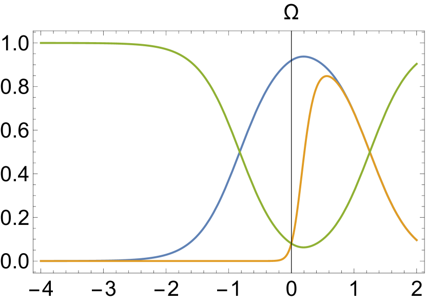
Fig. 2: Evolution of energy fractions as functions of $y=ln(a)$, for $Z=0.022$. Matter dominates early cosmology, with $\Omega_{E}$ (green curve) close to one. For $y>-2$ the dark energy fraction $\Omega_{h}$ (blue curve) starts to increase. At present ($y=0$) it is dominated by the potential, as visible from the small $\Omega_{K}$ (orange curve).

As one further increases $x(y_{\text{in}})$ slightly, dark energy becomes important earlier, and also the decrease of $\Omega_{h}$ and increase of $\Omega_{K}$ begin at smaller $y$. One can tune $x(y_{\text{in}})$ in order to obtain a given $\Omega_{h}(0)$. For $x(y_{\text{in}})=-4.04219658$ the evolution is shown for $\Omega_{h}$, $\Omega_{K}$ and $\Omega_{E}$ in fig. 3. The present dark energy fraction $\Omega_{h}(0)=0.7$ would be consistent with observation. At $y=0$ the dark energy (blue curve) is dominated by the cosmon kinetic energy (orange curve), resulting in an equation of state $w_{h}(0)\approx 1$. This is not compatible with observation. The present value of the Hubble parameter obtains from $y(0)=0.0022$ very close to $H_{0}$.

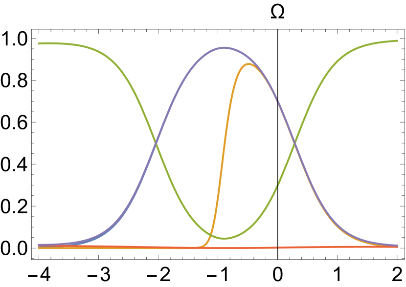
Fig. 3: Evolution of energy fractions as function of $y=\ln a$ for $Z=0.022$. The color coding is the same as for Fig. 2. The present dark energy fraction is $\Omega_{h}=0.7$, with equation of state $w_{h}(0)$ close to one. The dynamics is similar to Fig. 2, but shifted in $y$.

We draw three main conclusions from this investigation. First, for the scaling solution of quantum gravity with constant neutrino masses in the Einstein frame the overall features of cosmology look qualitatively similar to a typical universe with thawing dark energy, provided $Z$ is in a suitable range. Second, the precise values of $\Omega_{h}(0)$ and $w_{h}(0)$ conflict with observation. Third, with our given assumptions the scaling solution of quantum gravity is predictive. Besides the neutrino masses and $Z$ there is no free parameter available which could influence the outcome. For larger neutrino masses and somewhat different $Z$ the incompatibility with observation does not change.

There are several ways how the cosmology corresponding to the scaling solution of quantum gravity can be modified. First, the scaling solution may be more complex than the one following from our simple truncation or assumptions. For the scaling solution the kinetial $K$ is a function of the dimensionless scale invariant scalar field $\tilde{\chi}=\chi/k$. The dependence of $K(\tilde{\rho})$ on $\tilde{\rho}$ may deviate from our truncation of constant $K$. In turn, this entails a non-trivial dependence of $Z(\varphi)$ on $\varphi$. We keep here $Z$ fixed and focus rather on the possibility that the scaling form of the effective neutrino Yukawa couplings $h_{\nu}(\tilde{\rho})$ depends on $\tilde{\rho}$ non-trivially. We will see that this can lead to growing neutrino quintessence [16, 17].

Second, the solution of the flow equation may deviate from the scaling solution. This implies the presence of relevant parameters and intrinsic mass scales associated to them. The largest intrinsic mass scale may be denoted by $\bar{k}$. As a consequence, the scaling solution holds to a good approximation for $k\gg\bar{k}$, while substantial deviations from the scaling solution occur for $k\leq\bar{k}$. The maximal intrinsic mass scale is a free parameter which sets the overall scale. We take it in the vicinity of $2\cdot 10^{-3}\,\text{eV}$. The effective squared Planck mass will then be dominated by $M^{2}\approx\xi\chi^{2}$, with only a tiny correction $\sim\bar{k}^{2}$. For the scaling potential $U=uk^{4}$ one expects more substantial modifications, for example by an additional constant $\bar{k}^{4}$. A discussion of this possibility is postponed to future work.

Scale symmetry violation in the neutrino sector

Let us consider the possibility that the effective neutrino Yukawa coupling $h_{\nu}(\tilde{\rho})$ shows a non-trivial dependence on $\tilde{\rho}$. The masses of the left-handed neutrinos of the standard model of particle physics arise from non-renormalizable couplings, which are sensitive to some “beyond standard model” (BSM) sector. A non-trivial $\tilde{\rho}$-dependence of the scaling solution in the BSM-sector, besides the proportionality of mass scales to $\chi$ according to quantum scale symmetry, can result in non-trivial $h_{\nu}(\tilde{\rho})$. Thus $\partial_{\tilde{\rho}}h_{\nu}(\tilde{\rho})\neq 0$ indicates a violation of quantum scale symmetry for the scaling solution in the BSM-sector.

If the characteristic $\chi$-dependent mass scales in the BSM-sector are much larger than the Fermi scale (expectation value of the Higgs doublet $\varphi_{0}\sim\chi$), the neutrino masses are small as compared to the electron mass due to some “seesaw mechanism” or “cascade mechanism”. They are suppressed either by the mass of a “right-handed” or “sterile” neutrino [37, 38, 39], or by the mass of a scalar triplet [40, 41]. If one of these masses is not exactly proportional to $\chi$, the quantum scale symmetry in the BSM-sector is violated. We make here the simplified assumption that this scale symmetry violation is common to all three neutrino masses and parameterize

$$m_{\nu}=b_{\nu}\frac{\varphi_{0}^{2}(\chi)}{m_{\text{B}-\text{L}}(\chi)}=\frac{b_{\nu}\varepsilon\chi^{2}}{g_{\text{B}-\text{L}}(\chi)\chi}\ ,$$ (53)

with constant $b_{\nu}$. Here $\varphi_{0}$ is the doublet expectation value, $\varphi_{0}^{2}=\varepsilon\chi^{2}$, and $m_{\text{B}-\text{L}}(\chi)=g_{\text{B}-\text{L}}(\chi)\chi$ is the heavy mass scale associated to $\text{B}-\text{L}$-violating effects in the BSM-sector. The effective coupling $g_{\text{B}-\text{L}}(\chi)$ incorporates the details of the mass-generation. For the scaling solution one has

$$h_{\nu}(\tilde{\rho})=\frac{b_{\nu}\varepsilon}{g_{\text{B}-\text{L}}(\tilde{\rho})}\ ,$$ (54)

such that a non-trivial $\tilde{\rho}$-dependence arises from the non-trivial $\tilde{\rho}$-dependence of $g_{\text{B}-\text{L}}(\tilde{\rho})$.

Typically, $g_{\text{B}-\text{L}}$ is some dimensionless combination of couplings, as the Yukawa coupling of the right-handed neutrinos, or quartic scalar couplings which determine the mass of the heavy triplet, a cubic coupling between the triplet and two doublets, or various expectation values. For a scaling solution which has not yet settled at some quantum scale invariant limit one could expect some logarithmic dependence on $\chi/k$, which we parameterize in the range of interest for $\tilde{\rho}$ by

$$g_{\text{B}-\text{L}}(\tilde{\rho})=\bar{g}_{\text{B}-\text{L}}-c_{\text{B}-\text{L}}\ln\left(\frac{\chi}{k}\right)\ .$$ (55)

(This parameterization is not supposed to be valid for $\tilde{\rho}\to 0$ or in a range where $g_{\text{B}-\text{L}}(\tilde{\rho})$ would vanish.) Translating to $\varphi$ yields

$$h_{\nu}(\varphi)=\frac{4b_{\nu}\varepsilon M}{4\bar{g}_{\text{B}-\text{L}}M-c_{\text{B}-\text{L}}\varphi}\ .$$ (56)

We consider positive $c_{\text{B}-\text{L}}$ and $g_{\text{B}-\text{L}}$ such that the neutrino masses in the Einstein frame increase with increasing $\varphi$.

The $\varphi$-dependence of the neutrino masses in the Einstein frame induces an effective coupling between the cosmon and neutrinos [16, 36],

$$\beta=-\frac{\partial\ln m_{\nu}}{\partial\varphi}M=-\frac{M}{\varphi_{c}-\varphi}=-\frac{1}{2(x_{c}-x)}\ ,$$ (57)

with

$$\frac{\varphi_{c}}{M}=\frac{4\bar{g}_{\text{B}-\text{L}}}{c_{\text{B}-\text{L}}}\ ,\quad x_{c}=\frac{\varphi_{c}-\bar{\varphi}}{2M}\ .$$ (58)

For a slow running, $c_{\text{B}-\text{L}}\ll\bar{g}_{\text{B}-\text{L}}$, the unknown parameter $\varphi_{c}/M$ may be in the range of the present value of $\varphi/M$, i.e. $\varphi_{c}$ close to $\bar{\varphi}$. In the limit $c_{\text{B}-\text{L}}\to 0$, $x_{c}\to\infty$ one has $\beta\to 0$ and recovers the case of the field-independent Yukawa coupling discussed previously. The cosmon-neutrino coupling has been employed in several models of dynamical dark energy with mass-varying neutrinos [42, 43, 44, 45, 46, 47, 48, 49].

The individual neutrino masses obey

$$m_{\nu}(\varphi)=\frac{\mu_{\nu}(\varphi_{c}-\varphi_{0})}{\varphi_{c}-\varphi}=\frac{\mu_{\nu}(x_{c}-x_{0})}{x_{c}-x}\ .$$ (59)

If we take for $\varphi_{0}$ the present value of $\varphi$, and correspondingly for $x_{0}$, the free parameters $\mu_{\nu}$ correspond to the present neutrino masses. In principle, one can choose $x_{0}$ arbitrarily. The free parameters in the neutrino sector are then $x_{c}$ and the three constant masses $\mu_{\nu}$, which together with $x_{0}$ define the neutrino masses for a given value of $\varphi$. In other words, $x_{c}$ is the only additional free parameter for this scenario. With $h_{\nu}(\varphi)=m_{\nu}(\varphi)\sqrt{\xi}/M$ one obtains for the scaling potential (18)

$$\tilde{m}_{\nu}^{2}(x)=\sqrt{\frac{u_{\infty}\mu_{\nu}^{4}}{U_{0}}}\left(\frac{x_{c}-x_{0}}{x_{c}-x}\right)^{2}\exp(x)\ .$$ (60)

A non-vanishing cosmon-neutrino coupling $\beta$ has several effects on the cosmology of the scaling solution. First, the evolution equation of the cosmon contains an additional term proportional to the trace of the energy-momentum tensor of the neutrinos

$$Z\big{(}\partial_{t}^{2}+3H\partial_{t}\big{)}\varphi=-\frac{\partial U_{E}}{\partial\varphi}+\frac{\beta}{M}(\rho_{\nu}-3p_{\nu})\ .$$ (61)

Second, the energy-momentum tensor of the neutrinos is not conserved, according to [50, 16],

$$\partial_{t}\rho_{\nu}+3H(\rho_{\nu}+p_{\nu})=-\frac{\beta}{M}(\rho_{\nu}-3p_{\nu})\partial_{t}\varphi\ .$$ (62)

Energy is exchanged between the neutrino- and cosmon-sector and only the combined energy momentum tensor for the scalar field and neutrinos is covariantly conserved,

$$\partial_{t}(\rho_{\nu}+\rho_{h})=-3H\big{(}\rho_{\nu}+p_{\nu}+Z(\partial_{t}\varphi)^{2}\big{)}\ .$$ (63)

Third, a variable neutrino mass influences the time when neutrinos get non-relativistic, i.e. when the neutrino pressure $p_{\nu}$ differs substantially from $\rho_{\nu}/3$. For negative $\beta$ and increasing neutrino masses neutrinos become non-relativistic later as compared to the case of constant neutrino masses. Only for non-relativistic neutrinos the modifications in eqs. (61), (62) matter.

Fourth, the scaling solution for the cosmon potential is modified since $\tilde{m}_{f}^{2}(\varphi)$ involves an additional factor

$$\frac{h_{\nu}^{2}(\varphi)}{h_{\nu}^{2}(\varphi_{0})} =\left(\frac{4\bar{g}_{\text{B}-\text{L}}M-c_{\text{B}-\text{L}}\varphi_{0}}{4\bar{g}_{\text{B}-\text{L}}M-c_{\text{B}-\text{L}}\varphi(t)}\right)^{2}$$

$$=\left(\frac{\varphi_{c}-\varphi_{0}}{\varphi_{c}-\varphi(t)}\right)^{2}=\left(\frac{x_{c}-x_{0}}{x_{c}-x}\right)^{2}\ .$$ (64)

This shifts the maximum of the potential, which now occurs for

$$\sum_{\nu}\left\{\frac{1}{1+\tilde{m}_{\nu}^{2}}-4\beta\left(\frac{1}{1+\tilde{m}_{\nu}^{2}}-t_{u}(\tilde{m}_{\nu}^{2})\right)\right\}=\frac{5}{2}\ .$$ (65)

With $(1+\tilde{m}_{\nu}^{2})^{-1}>t_{u}(\tilde{m}_{\nu}^{2})$, a negative value of $\beta$ shifts the potential maximum towards larger $\varphi$ or $x$. For $x_{c}=0.22$, $x_{0}=0.08$, $\bar{\mu}_{\nu}=0.422\,\text{eV}$ we plot the effective cosmon potential in fig. 4.

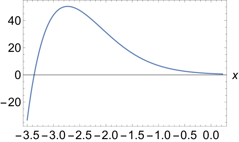
Fig. 4: Cosmon potential for running neutrino Yukawa coupling. We plot $U_{E}/U_{0}$ as function of $x=(\varphi-\bar{\varphi})/(2M)$ for the parameters $x_{c}=0.22$, $x_{0}=0.08$, $\bar{\mu}_{\nu}=\sum_{\nu}\mu_{\nu}/3=0.422\,\text{eV}$.

As compared to Fig. 1 the potential maximum is shifted to larger $x$ and its height is lower. For smaller $\mu_{\nu}$ these effects are enhanced. Fifth, the additional cosmon-mediated attractive force between neutrinos accelerates the growth of fluctuations in the neutrino-sector. In our approximation all these effects are governed by a single new parameter $x_{c}$, which determines the function $\beta(x)$ according to eq. (57).

Growing neutrino quintessence

For cosmology we have to take the effects of the neutrino fluid into account, with

$$\Omega_{\nu}=\frac{\rho_{\nu}}{3M^{2}H^{2}}\ ,\quad\Omega_{m}+\Omega_{V}+\Omega_{K}+\Omega_{\nu}+\Omega_{\gamma}=1\ .$$ (66)

Here $\Omega_{m}$ and $\Omega_{\gamma}$ are the fractions of matter and photons, corresponding to the energy densities with the usual scaling behavior $\rho_{m}\sim a^{-3}$, $\rho_{\gamma}\sim a^{-4}$. For the evolution of $\rho_{\nu}$ or $\Omega_{\nu}$ we need the effective equation of state in the neutrino-sector $w_{\nu}=p_{\nu}/\rho_{\nu}$. In addition to eq. (62) or (63) we will use

$$\rho_{\nu}-3p_{\nu}=\bar{m}_{\nu}n_{\nu}\ ,$$ (67)

with total number density of neutrinos $n_{\nu}\sim a^{-3}$, and average neutrino mass $\bar{m}_{\nu}$,

$$\bar{m}_{\nu}=\frac{1}{3}\sum_{\nu}m_{\nu}\ .$$ (68)

In early cosmology the neutrino masses are negligible, $w_{\nu}=1/3$, and $\rho_{\nu}\sim T_{\nu}^{4}$ is given by the effective neutrino temperature $T_{\nu}$. For the present epoch of cosmology $p_{\nu}$ is of the same order as the energy density of photons and therefore negligible, $w_{\nu}\approx 0$.

For the present cosmological epoch we may combine the cosmon and neutrino energy density into a common effective dark energy density $\rho_{d}$,

$$\rho_{d}=\rho_{\nu}+\rho_{h}=\rho_{\nu}+U_{E}+\frac{Z}{2}\big{(}\partial_{t}\varphi\big{)}^{2}\ .$$ (69)

Neglecting $p_{\nu}$ one has for late cosmology, with $\bar{\mu}_{\nu}=\frac{1}{3}\sum_{\nu}\mu_{\nu}$,

$$\partial_{t}\rho_{d} =-3H\left[\frac{\bar{\mu}_{\nu}n_{\nu}(\varphi_{c}-\varphi_{0})}{\varphi_{c}-\varphi}+Z\big{(}\partial_{t}\varphi\big{)}^{2}\right]$$

$$=-3(1+w_{d})H\rho_{d}\ .$$ (70)

The equation of state for this combined effective dark energy $w_{d}$ obeys for non-relativistic neutrinos

$$w_{d} =\frac{T-U_{E}}{T+U_{E}+\rho_{\nu}}\ ,\quad T=\frac{Z}{2}\big{(}\partial_{t}\varphi\big{)}^{2}\ ,$$

$$\rho_{\nu} =\frac{\varphi_{c}-\varphi_{0}}{\varphi_{c}-\varphi}\bar{\mu}_{\nu}n_{\nu}\ .$$ (71)

It is restricted by $w_{d}>-1$, coming close to $(-1)$ if $T$ and $\rho_{\nu}$ are small as compared to $U_{E}$.

For a numerical solution we employ the field equation

$$\partial_{y}^{2}x+(3+\partial_{y}g)\partial_{y}x$$

$$=\frac{3}{2Z}\left[\left(1-\frac{1}{2}\partial_{x}\ln u\right)\Omega_{V}-\frac{\Omega_{\nu}(1-3w_{\nu})}{2(x_{c}-x)}\right]\ ,$$ (72)

where we insert

$$\partial_{y}g=-\frac{3}{2}\big{(}1+w_{\nu}\Omega_{\nu}+\Omega_{K}-\Omega_{V}\big{)}-\frac{1}{2}\Omega_{\gamma}\ .$$ (73)

Here $\Omega_{V}$ and $\Omega_{K}$ are given by eqs. (46) and (42), respectively. The factor $1-3w_{\nu}$ suppresses the effects of the cosmon-neutrino coupling as long as the neutrinos are relativistic. Using $n_{\nu}\sim a^{-3}$ we employ

$$\Omega_{\nu}(1-3w_{\nu}) =\frac{\bar{m}_{\nu}n_{\nu}}{3M^{2}H^{2}}$$

$$=\frac{\bar{\mu}_{\nu}B}{3M^{2}H_{0}^{2}}\exp\big{\{}-(3y+2g)\big{\}}\frac{x_{c}-x_{0}}{x_{c}-x}\ ,$$

with

$$B=n_{\nu}(y_{\text{in}})\exp(3y_{\text{in}})=\frac{4c_{\nu}}{11}T_{\gamma,0}^{3}\ ,$$ (74)

where $T_{\gamma,0}=2.348\cdot 10^{-4}\,\text{eV}$ is the present photon temperature and $c_{\nu}\approx 0.548$, see below. The evolution of the neutrino fraction obeys

$$\partial_{y}\Omega_{\nu}=-\Omega_{\nu}\left[4+2\partial_{y}g-\left(1+\frac{\partial_{y}x}{x_{c}-x}\right)\big{(}1-3w_{\nu}\big{)}\right]\ .$$ (75)

A rather robust numerical approach follows directly the evolution of $\rho_{m}$, $\rho_{\gamma}$ and $\rho_{\nu}$ in addition to the scalar field $x$ given by eq. (Growing neutrino quintessence). This yields the evolution of the critical energy density $3M^{2}H^{2}=\rho_{m}+\rho_{\gamma}+\rho_{\nu}+\rho_{h}$ and therefore of $g(y)$.

We need to determine the initial conditions, which we choose typically at $a_{\text{in}}=1/3000$ near matter-radiation equality. The initial neutrino number density $n_{\nu}(y_{\text{in}})$ is given by ($\zeta(3)=1.202$)

$$n_{\nu}(y_{\text{in}})=c_{\nu}T_{\nu}^{3}(y_{\text{in}})\ ,\quad c_{\nu}=\frac{9\zeta(3)}{2\pi^{2}}=0.548\ .$$ (76)

Here the neutrino temperature $T_{\nu}$ is related to the photon temperature $T_{\gamma}$

$$T_{\nu}=\left(\frac{4}{11}\right)^{\frac{1}{3}}T_{\gamma}=\left(\frac{4}{11}\right)^{\frac{1}{3}}T_{\gamma,0}\exp(-y)\ .$$ (77)

This yields eq. (74) and implies for the scalar evolution equation

$$\Omega_{\nu}(1-3w_{\nu})=D\frac{\bar{\mu}_{\nu}(x_{c}-x_{0})}{1\,\text{eV}}\frac{\exp\big{(}-(3y+2g)\big{)}}{(x_{c}-x)}\ ,$$ (78)

with

$$D=\frac{4c_{\nu}T_{\gamma,0}^{3}(1\,\text{eV})}{33M^{2}H_{0}^{2}}=0.0657\ .$$ (79)

In turn, we can use

$$w_{\nu}\Omega_{\nu}=\frac{1}{3}\Omega_{\nu}-\frac{1}{3}\big{(}1-3w_{\nu}\big{)}\Omega_{\nu}\ .$$ (80)

For the photon fraction we employ

$$\Omega_{\gamma}=\frac{\pi^{2}T_{\gamma,0}^{4}}{45M^{2}H_{0}^{2}}\exp\big{(}(-(4y+2g)\big{)}\ .$$ (81)

For the initial value of $g(y_{\text{in}})$ we need the contribution of photons and neutrinos to the energy density at $y_{\text{in}}$, as determined for an early epoch where neutrino masses are negligible by

$$\Omega_{r}(a)=\Omega_{\gamma}(a)+\Omega_{\nu}(a)=\frac{a_{\text{eq}}}{a+a_{\text{eq}}}\ ,$$ (82)

with matter-radiation equality at $a_{\text{eq}}=1/3390$. For $y_{\text{in}}=\ln(1/3000)$ this yields the total radiation fraction $\Omega_{r}(y_{\text{in}})=0.47$. The initial value for $g$ is given by

$$g(y_{\text{in}})= \,-\frac{3y_{\text{in}}}{2}+\frac{1}{2}\ln\big{(}1-\Omega_{d,0}\big{)}$$

$$-\frac{1}{2}\ln\big{(}1-\Omega_{r}(y_{\text{in}})-\Omega_{h}(y_{\text{in}})\big{)}\ ,$$ (83)

Here $\Omega_{d,0}$ is the present total dark energy fraction which sums the cosmon potential and kinetic energy, as well as the energy density of neutrinos. For $\Omega_{d,0}=0.7$ this amounts to $g(y_{\text{in}})=11.708$. The value of $g(y_{\text{in}})$ has to be adapted to match the outcome of $\Omega_{d,0}$.

For the initial value of $\Omega_{\nu}$ we use that the neutrino masses are negligible in early cosmology such that

$$\frac{\Omega_{\nu}}{\Omega_{\gamma}}=c_{\nu\gamma}=\frac{21}{8}\left(\frac{4}{11}\right)^{\frac{4}{3}}\ ,\quad\Omega_{\nu}=\frac{c_{\nu\gamma}}{1+c_{\nu\gamma}}\Omega_{r}\ ,$$ (84)

and

$$\Omega_{\nu}(y)=\frac{c_{\nu\gamma}a_{\text{eq}}}{(1+c_{\nu\gamma})(e^{y}+a_{\text{eq}})}\ .$$ (85)

For $y_{\text{in}}=\ln(1/3000)$ one finds the initial value $\Omega_{\nu}(y_{\text{in}})=0.19$.

The evolution equation (Growing neutrino quintessence) for $g$ implies that $\rho_{m}$, as defined by $\Omega_{m}=1-(\Omega_{h}+\Omega_{\nu}+\Omega_{\gamma})$, scales $\sim a^{-3}$. For numerical robustness we rather implement directly this relation by

$$\rho_{m}(y)=\rho_{m,0}\exp(-3y)\ ,$$ (86)

with $\rho_{m,0}$ determined from the scale factor at radiation-matter equality as

$$\rho_{m,0}=(1+c_{\nu\gamma})\rho_{\gamma,0}a_{\text{eq}}^{-1}\ ,\quad\rho_{\gamma,0}=\frac{\pi^{2}}{15}T_{\gamma,0}^{4}.$$ (87)

For the epoch when the neutrino masses are negligible this yields an approximate expression for $g(y)$,

$$g(y)=\frac{1}{2}\bigg{[} \ln\big{(}\rho_{m,0}e^{-3y}+\rho_{\gamma,0}(1+c_{\nu\gamma})e^{-4y}+\rho_{h}\big{)}$$

$$- \ln\big{(}3M^{2}H_{0}^{2}\big{)}\bigg{]}\ .$$ (88)

We actually use this expression for the determination of $g(y_{\text{in}})$, which yields results very close to eq. (81). Extending the discussion to the energy density of a free gas of massive neutrinos, one obtains an explicit equation for $g$ in terms of $y$, $x(y)$ and $\partial_{y}x(y)$,

$$\exp(2g)\left(1-\frac{2Z}{3}(\partial_{y}x)^{2}\right)=\big{(}3M^{2}H_{0}^{2}\big{)}^{-1}$$

$$\times\Big{[}\rho_{\gamma,0}\big{(}e^{-4y}+(1+c_{\nu\gamma})e^{-3y}a_{\text{eq}}^{-1}\big{)}+\rho_{\nu}+U_{E}\Big{]}\ .$$ (89)

For a numerical solution of the system of differential equations we treat $x(y_{\text{in}})$ as a free parameter, set by the evolution of the scalar field prior to $y_{\text{in}}$. We find that the evolution is rather independent of the initial condition for $\partial_{y}x(y_{\text{in}})$. After a rather short initial period $\partial_{y}x$ settles at a scaling behavior. We take $(\partial_{y}x)(y_{\text{in}})=0$ as second initial condition. The initial conditions for $g(y_{\text{in}})$ and $\Omega_{\nu}(y_{\text{in}})$ are fixed by eqs. (Growing neutrino quintessence) (85).

A typical numerical solution for $Z=0.022$, $x_{c}=0.22$, $\bar{\mu}_{\nu}=0.422\,\text{eV}$, $x_{0}=0.08$ and initial value $x(y_{\text{in}})=-2.78$ shows the onset of an oscillatory behavior once the neutrinos get non-relativistic. Asymptotically for large $y$ the universe turns to a dark energy dominated universe. The present epoch at $y=0$ is situated in a transition epoch. In fig. 5 we display the evolution of the dimensionless scalar field $x$ as a function of $y=\ln a$.

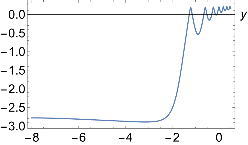
Fig. 5: Evolution of the dimensionless scalar field $x=(\varphi-\bar{\varphi})/(2M)$ as function of $y=\ln a$. Parameters are $Z=0.022$, $x_{c}=0.22$, with neutrino masses determined by $\bar{\mu}_{\nu}=0.422\,\text{eV}$, $x_{0}=0.08$. For $x(y_{\text{in}})=-2.78$ at $y_{\text{in}}=-\ln(3000)$ the cosmon neutrino coupling is small initially and induces a slow decrease of $x$. As the universe expands the relative importance of the potential gradient increases, reversing the evolution of $x$ towards a rapid increase near $y=-2$. Subsequently, the scalar field follows an oscillatory approach towards $x_{c}$.

The neutrino-induced force $\sim\beta$ first drives $x$ slowly towards smaller values. The values of $x$ shown in the figure correspond to the tail of the scalar potential at the right of the maximum in fig. 4. At some moment the gradient of the potential overtakes and $x$ is pushed to larger values again. The competition between the neutrino-induced and gradient force, which have opposite sign, results in an oscillatory behavior. For $y$ increasing to the future ($y>0$) the scalar field essentially approaches a constant. The scalar potential $U_{E}(x)$ therefore becomes almost constant, which can be identified with an effective cosmological constant.

This overall behavior is reflected in the evolution of the different energy densities or corresponding energy fractions $\Omega_{m}$, $\Omega_{d}$, $\Omega_{h}$, $\Omega_{K}$ and $\Omega_{\nu}$ shown in fig. 6.

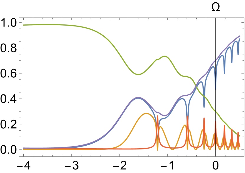
Fig. 6: Evolution of energy fractions for $Z=0.022$, $x_{c}=0.22$, $x(y_{\text{in}})=-2.78$, $y_{\text{in}}=-\ln(3000)$. All parameters are the same as for Fig. 5. For the range $y\approx-4$ the universe is dominated by matter, with $\Omega_{m}$ (green curve) close to one. For $y\approx-2$ the cosmon potential starts to matter, leading to an increase of $\Omega_{h}$ (blue curve). In this epoch the scalar kinetic energy $\Omega_{K}$ (orange curve) and the neutrino energy $\Omega_{\nu}$ (red curve) are small, such that the combined dark energy fraction $\Omega_{d}$ (violet curve) almost coincides with $\Omega_{h}$. Subsequently, the rapid increase of $x$ leads to an increase of $\Omega_{K}$. Whenever $x$ comes close to $x_{c}$ the neutrino fraction $\Omega_{\nu}$ shows spikes due to the enhanced neutrino masses. These spikes in $\Omega_{\nu}$ are accompanied by drops in $\Omega_{h}$, while $\Omega_{d}$ shows a relatively smooth increase, with present value $\Omega_{d}(0)=0.7$.

In early cosmology matter and radiation dominate. For the range $y\approx-4$ shown in the figure the universe is matter dominated with $\Omega_{m}$ (green) close to one. Around $y\approx-2.5$ the cosmon potential starts to play a role, inducing an increase of $\Omega_{V}$. As long as the field value changes slowly – its direction being reversed near $y=-3$ – the kinetic energy fraction $\Omega_{K}$ (orange) remains small, such that $\Omega_{h}\approx\Omega_{V}$. Also the neutrino energy fraction $\Omega_{\nu}$ (red) is small, such that the curves for $\Omega_{h}$ (blue) and $\Omega_{d}$ (violet) almost coincide. Subsequently, after $y=-2$ the potential gradient induces a rapid increase of $x$. This is the moment when dark energy ”thaws”, as visible in the increase of the kinetic energy fraction $\Omega_{K}$ (orange). The thawing is stopped, however, once $x$ approaches $x_{c}$. The strong cosmon-neutrino coupling $\beta$ counteracts the further increase of $x$ and reverses the sign of $\partial_{y}x$ (sharp drop in $\Omega_{K}$, orange). The cosmon field decreases again, until the potential gradient takes over. The oscillations of $x$ are visible in the oscillations of $\Omega_{h}$ (blue). The sharp drops in $\Omega_{h}$ are partly compensated by sharp peaks in $\Omega_{\nu}$ which occur whenever $x$ is close to $x_{c}$. While $\Omega_{h}$ and $\Omega_{\nu}$ oscillate strongly due to the oscillating scalar field $x$, the combined dark energy fraction $\Omega_{d}$ is a more smooth function. After a first drop around $y=-1$ it increases monotonically, still showing small oscillations. For the parameters chosen $\Omega_{d}$ reaches a value $\Omega_{d}(0)=0.7$. In summary, the thawing is not smooth as for $\beta=0$. The increase of $\Omega_{d}$, and the corresponding decrease of $\Omega_{m}$, show structures which clearly distinguish the evolution from a cosmological constant. In particular, the drop of $\Omega_{d}$ near $y=-1$ could be an observable signature for this setting.

In fig. 7 we show the equation of state for the scalar field energy density $w_{h}$, as well as the effective equation of state $w_{d}$ for the combined neutrino-cosmon fluid.

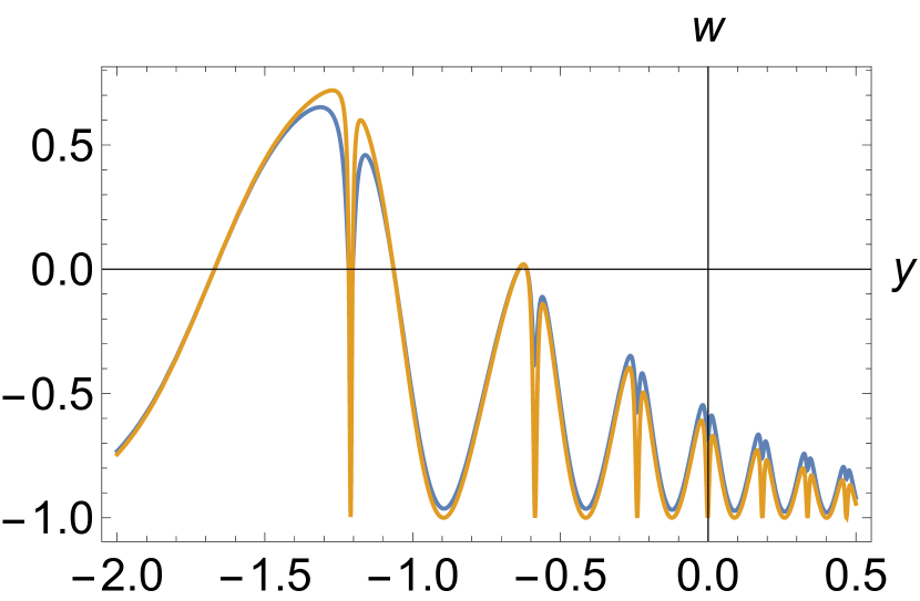
Fig. 7: Equation of state of scalar field dark energy (orange) and combined neutrino + scalar dark energy (blue) as function of $y=\ln a$. Parameters are the same as for Figs. 5.

For the scalar field $w_{h}$ starts in early cosmology close to $w_{h}=-1$, corresponding to the dominance of the potential. Near $y=-1.5$ it turns to a positive value, indicating the dominance of kinetic energy over potential energy. Subsequently, the equation of state decreases in an oscillating way towards $w_{h}=-1$. We show both the equation of state of the scalar field dark energy $w_{h}$ (orange) and the equation of state for the combined dark energy $w_{d}$ (blue). The presence of $\rho_{\nu}$ in the denominator of eq. (Growing neutrino quintessence) reduces somewhat the peaks of the oscillations. For the parameters chosen one has at present $w_{h}(0)=-0.98$ and $w_{d}(0)=-0.68$. The oscillatory behavior of the equation of state is a characteristic signature for our setting. A given observation will presumably not resolve it fully, but rather result in some type of averaging. The equation of state depends on the neutrino masses. For smaller $\bar{\mu}_{\nu}$ it typically gets closer to $w_{d}=-1$.

The evolution of the average neutrino mass is displayed in fig. 8.

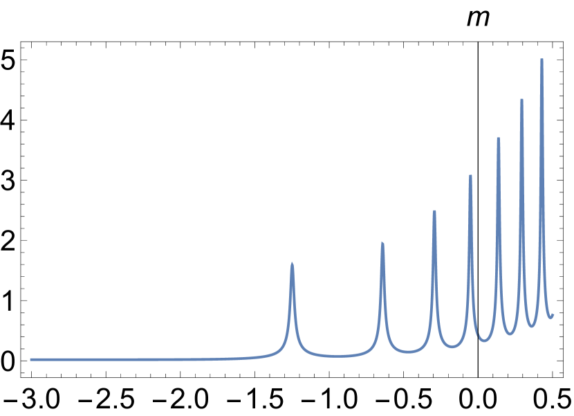
Fig. 8: Evolution of average neutrino mass $\bar{m}_{\nu}$ in units of  eV as function of $y=\ln a$. The precise location of the peaks depends on the parameters and initial conditions, given here by the ones of Fig. 5.

We observe the tendency of growing neutrino masses as $x$ approaches $x_{c}$. The evolution of the neutrino masses is strongly oscillating, with rather sharp peaks at the turning points for the evolution of the scalar field near $x_{c}$. The present average neutrino mass for our particular set of parameters and initial conditions is $\bar{m}_{\nu}=0.428\,\text{eV}$. The precise value is highly sensitive to the details in view of the strong oscillations. The relatively large value of the present neutrino mass is not in contradiction with cosmological observations. During structure formation the neutrino masses have been much smaller. For example, one has $\bar{m}_{\nu}(y=-3)=0.019\,\text{eV}$.

Despite the oscillatory behavior the evolution of the Hubble parameter is rather smooth. We display $h$ as a function of $y$ in fig. 9.

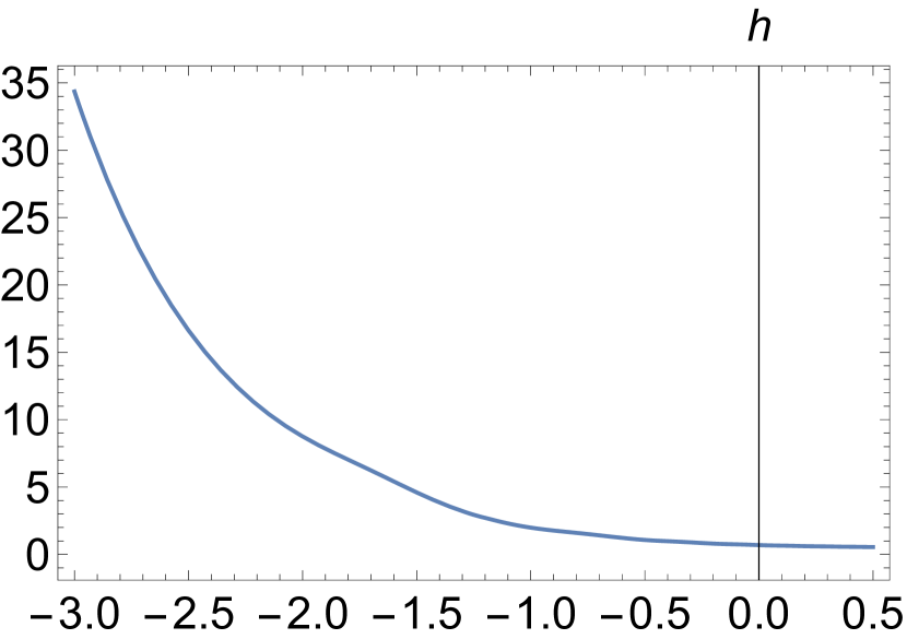
Fig. 9: Evolution of the dimensionless Hubble parameter $h$ as function of $y=\ln a$. Parameters and initial conditions are the same as for Fig. 5.

For our parameters and initial conditions the present value is found $h(0)=0.69$. For other settings $h(0)$ may come out larger than $0.7$.

From the overall oscillating picture it is evident that the detailed value of observables today depend sensitively on the value of $x_{c}$ and the initial value $x(t_{\text{in}})$, as given by the parameter $Z$ for a given inflationary cosmology and subsequent entropy production and heating. In the plane $(x_{c},x(t_{\text{in}}))$ one finds a line for which the present combined dark energy fraction $\Omega_{d}$ amounts to $0.7$. The present distribution of this combined dark energy on the cosmon potential, cosmon kinetic energy and neutrino energy density is parameter-dependent. This is seen by the fast oscillations between these components, and reflected in the oscillating equation of state. Furthermore, the oscillations depend strongly on the assumed neutrino masses as encoded in $\bar{\mu}$ and $x_{0}$. For smaller $\bar{\mu}$ the oscillations get faster, which renders a precise numerical solution more delicate. For smaller neutrino masses the present fraction of neutrino energy density and kinetic cosmon energy become smaller. The evolution of the potential energy gets smoother in recent cosmology, and the equation of state becomes even closer to $w_{d}=-1$.

We have chosen $x(y_{\text{in}})$ in a range where the effect of the cosmon-neutrino coupling $\beta$ is not large. The situation changes if the increase of $x$ during the early kination epoch drives $x$ to values close to $x_{c}$. Then the cosmon-neutrino coupling $\beta$ may become important earlier, changing the detailed dynamics. We recall here that our approximations for $\beta$ are not supposed to hold for $x$ very close to $x_{c}$ or larger than $x_{c}$.

A detailed search in parameter space will be necessary in order to find out if there exists a parameter region for which the model is compatible with all present observations, possibly overcoming the tensions in the cosmological constant model. This investigation is not the purpose of the present note. Furthermore, we should mention that in growing neutrino quintessence the neutrino fluctuations grow non-linear in a recent cosmological epoch. The neutrinos form very large lumps, which may render the cosmic neutrino background observable by large scale inhomogeneities in the gravitational potential. Rather large backreaction effects are possible. Also the locally observed Hubble parameter may deviate from its cosmological average, with possible implications for the Hubble tension. For small neutrino masses these effects are suppressed by the small neutrino fraction $\Omega_{\nu}$. Nevertheless, they could play a certain role for a detailed quantitative analysis. We refer to refs [51, 52, 53, 54, 55, 56, 57] for a detailed discussion of these issues.

Conclusions

In this note we have investigated the consequences of the scaling solution for quantum gravity for the evolution of dynamical dark energy. Our main assumption is that the largest intrinsic mass scale produced by running dimensionless couplings is of the order of a few meV, rather than the Planck scale as often assumed. This leads to models of variable gravity and a scale symmetric standard model. The scaling solution of quantum gravity predicts a very light scalar field – the cosmon – as the pseudo Goldstone boson of spontaneously broken quantum scale symmetry. For suitable parameters, i.e. an appropriate range for $Z$, the evolution of the cosmon field induces dynamical dark energy. This is a striking prediction. It will be crucial to find out if the required value of $Z$ is compatible with the scaling solution for the scalar kinetic term.

The second central outcome states that the scaling solution of quantum gravity is highly predictive for cosmology. This is due to the fact that the particles of the standard model and their interactions are well known, such that the flow equations contain essentially no free parameters for the relevant values of the cosmon field. Without a violation of quantum scale symmetry in the beyond standard model sector the time evolution of dynamical dark energy is not compatible with the precise cosmological constraints. In contrast, the simple assumption of a slow logarithmic running in the beyond standard model sector leads to models of growing neutrino quintessence. The rich and interesting phenomenology of these models may well be compatible with observation. For further progress in this direction one needs to identify which type of fluctuations lead to a scale violation in the beyond standard model sector.

We have focused in this note on exact scaling solutions of quantum gravity according to fundamental scale invariance [58]. It is remarkable that this very restrictive setting may lead to a cosmology compatible with observation. Relevant parameters for the flow away from the scaling solution could induce a small number of additional parameters for the cosmon potential, which will need to be investigated.

Our discussion of late dynamical dark energy has to be combined with an investigation of the inflationary epoch. Inflation is also predicted by the scaling solution of quantum gravity. The details of the inflationary epoch will depend, however, on unknown particles with high masses, as for grand unified models. For a given particle content the scaling solution of quantum gravity is very predictive for inflation as well. It seems conceivable that the kinetial of the cosmon, as reflected by $Z$, stops to evolve for large $\chi$ once the metric fluctuations and heavy particles have decoupled. The value of $Z$ may then depend again on assumptions for unknown particles, whose fluctuations determine its value for small $\chi$.

It is often believed that quantum gravity effects only affect very early cosmology. In contrast, our findings reveal that quantum gravity can also be very predictive for late cosmology. The severe constraints on the existence of scaling solutions for all values of the cosmon field fix the scaling solution for the cosmon potential. This potential is a key ingredient for the dynamics of dark energy. It can no longer be assumed ad hoc for phenomenological purposes, but rather becomes a calculable quantity. We hope that a large and fruitful research field emerges from this combination of cosmology with quantum gravity.

References

- Wetterich [1988a] C. Wetterich, Cosmology and the fate of dilatation symmetry, Nuclear Physics B 302, 668–696 (1988a), arXiv:1711.03844 .
- Wetterich [2019] C. Wetterich, Quantum scale symmetry (2019), arXiv:1901.04741 [hep-th] .
- Weinberg [1980] S. Weinberg, Ultraviolet divergences in quantum theories of gravitation, in General Relativity: an Einstein Centenary Survey (Cambridge University Press, 1980) p. 790.
- Reuter [1998] M. Reuter, Nonperturbative evolution equation for quantum gravity, Phys. Rev. D 57, 971 (1998), arXiv:hep-th/9605030 [hep-th] .
- Stelle [1977] K. S. Stelle, Renormalization of higher-derivative quantum gravity, Phys. Rev. D 16, 953 (1977).
- Fradkin and Tseytlin [1982] E. S. Fradkin and A. A. Tseytlin, Renormalizable asymptotically free quantum theory of gravity, Nucl. Phys. B 201, 469 (1982).
- Avramidy and Barvinsky [1985] I. G. Avramidy and A. O. Barvinsky, Asymptotic freedom in higher-derivative quantum gravity, Phys. Lett. B 159, 269 (1985).
- Sen et al. [2022] S. Sen, C. Wetterich, and M. Yamada, Asymptotic freedom and safety in quantum gravity, JHEP 03, 130, arXiv:2111.04696 [hep-th] .
- Wetterich [2022] C. Wetterich, The Quantum Gravity Connection between Inflation and Quintessence, Galaxies 10, 50 (2022), arXiv:2201.12213 [astro-ph.CO] .
- Wetterich [2023] C. Wetterich, Quantum gravity and scale symmetry in cosmology (2023), arXiv:2211.03596 [gr-qc] .
- Wetterich [2014] C. Wetterich, Variable gravity universe, Phys. Rev. D 89, 024005 (2014), arXiv:1308.1019 [astro-ph.CO] .
- Henz et al. [2017] T. Henz, J. Pawlowski, and C. Wetterich, Scaling solutions for dilaton quantum gravity, Physics Letters B 769, 105 (2017), arXiv:1605.01858 .
- Henz et al. [2013] T. Henz, J. Pawlowski, A. Rodigast, and C. Wetterich, Dilaton quantum gravity, Physics Letters B 727, 298–302 (2013), arXiv:1304.7743 .
- Shaposhnikov and Zenhäusern [2009a] M. Shaposhnikov and D. Zenhäusern, Scale invariance, unimodular gravity and dark energy, Physics Letters B 671, 187–192 (2009a), arXiv:0809.3395 [hep-th] .
- Shaposhnikov and Zenhäusern [2009b] M. Shaposhnikov and D. Zenhäusern, Quantum scale invariance, cosmological constant and hierarchy problem, Physics Letters B 671, 162 (2009b), arXiv:0809.3406 [hep-th] .
- Wetterich [2007] C. Wetterich, Growing neutrinos and cosmological selection, Physics Letters B 655, 201–208 (2007), arXiv:0706.4427 [hep-ph] .
- Amendola et al. [2008] L. Amendola, M. Baldi, and C. Wetterich, Quintessence cosmologies with a growing matter component, Physical Review D 78 (2008), arXiv:0706.3064 [astro-ph] .
- Pawlowski et al. [2019] J. M. Pawlowski, M. Reichert, C. Wetterich, and M. Yamada, Higgs scalar potential in asymptotically safe quantum gravity, Physical Review D 99 (2019), arXiv:1811.11706 [hep-th] .
- Wetterich [2020] C. Wetterich, Effective scalar potential in asymptotically safe quantum gravity, Universe 7, 45 (2020), arXiv:1911.06100 [hep-th] .
- Dou and Percacci [1998] D. Dou and R. Percacci, The running gravitational couplings, Classical and Quantum Gravity 15, 3449–3468 (1998), arXiv:hep-th/9707239 .
- Narain and Percacci [2010] G. Narain and R. Percacci, Renormalization group flow in scalar-tensor theories: I, Classical and Quantum Gravity 27, 075001 (2010), arXiv:0911.0386 [hep-th] .
- Percacci and Vacca [2015] R. Percacci and G. P. Vacca, Search of scaling solutions in scalar–tensor gravity, The European Physical Journal C 75 (2015), arXiv:1501.00888 [hep-th] .
- Donà et al. [2016] P. Donà, A. Eichhorn, P. Labus, and R. Percacci, Asymptotic safety in an interacting system of gravity and scalar matter, Physical Review D 93 (2016), arXiv:1512.01589 [hep-th] .
- Eichhorn et al. [2018] A. Eichhorn, Y. Hamada, J. Lumma, and M. Yamada, Quantum gravity fluctuations flatten the planck-scale higgs potential, Physical Review D 97 (2018), arXiv:1712.00319 [hep-th] .
- Eichhorn and Pauly [2021] A. Eichhorn and M. Pauly, Constraining power of asymptotic safety for scalar fields, Physical Review D 103 (2021), arXiv:2009.13543 [hep-th] .
- Laporte et al. [2021] C. Laporte, A. D. Pereira, F. Saueressig, and J. Wang, Scalar-tensor theories within asymptotic safety, Journal of High Energy Physics 2021 (2021), arXiv:2110.09566 [hep-th] .
- Wetterich [1993] C. Wetterich, Exact evolution equation for the effective potential, Physics Letters B 301, 90–94 (1993), arXiv:1710.05815 [hep-th] .
- Reuter and Wetterich [1994] M. Reuter and C. Wetterich, Effective average action for gauge theories and exact evolution equations, Nucl. Phys. B 417, 181 (1994).
- Dupuis et al. [2021] N. Dupuis, L. Canet, A. Eichhorn, W. Metzner, J. Pawlowski, M. Tissier, and N. Wschebor, The nonperturbative functional renormalization group and its applications, Physics Reports 910, 1–114 (2021), arXiv:2006.04853 [cond-mat.stat-mech] .
- Wetterich [2018] C. Wetterich, Gauge invariant flow equation, Nuclear Physics B 931, 262 (2018), arXiv:1607.02989 [hep-th] .
- Wetterich [2017] C. Wetterich, Graviton fluctuations erase the cosmological constant, Physics Letters B 773, 6–19 (2017), arXiv:1704.08040 [gr-qc] .
- Litim [2001] D. F. Litim, Optimized renormalization group flows, Physical Review D 64 (2001), arXiv:hep-th/0103195 .
- Wetterich [2024] C. Wetterich, Simplified functional flow equation (2024), arXiv:2403.17523 [hep-th] .
- Wetterich and Yamada [2019] C. Wetterich and M. Yamada, Variable planck mass from the gauge invariant flow equation, Physical Review D 100 (2019), arXiv:1906.01721 [hep-th] .
- Linder [2007] E. V. Linder, The dynamics of quintessence, the quintessence of dynamics, General Relativity and Gravitation 40, 329–356 (2007), arXiv:0704.2064 [astro-ph] .
- Wetterich [1994] C. Wetterich, The cosmon model for an asymptotically vanishing time-dependent cosmological “constant” (1994), arXiv:hep-th/9408025 .
- Minkowski [1977] P. Minkowski, → at a rate of one out of 109 muon decays?, Physics Letters B 67, 421 (1977).
- Yanagida [1979] T. Yanagida, Horizontal gauge symmetry and masses of neutrinos, Conf. Proc. C 7902131, 95 (1979).
- Gell-Mann et al. [1979] M. Gell-Mann, P. Ramond, and R. Slansky, Complex Spinors and Unified Theories, Conf. Proc. C 790927, 315 (1979), arXiv:1306.4669 [hep-th] .
- Magg and Wetterich [1980] M. Magg and C. Wetterich, Neutrino mass problem and gauge hierarchy, Physics Letters B 94, 61 (1980).
- Lazarides et al. [1981] G. Lazarides, Q. Shafi, and C. Wetterich, Proton lifetime and fermion masses in an so(10) model, Nuclear Physics B 181, 287 (1981).
- Gu et al. [2003] P. Gu, X. Wang, and X. Zhang, Dark energy and neutrino mass limits from baryogenesis, Phys. Rev. D 68, 087301 (2003), arXiv:hep-ph/0307148 .
- Fardon et al. [2004] R. Fardon, A. E. Nelson, and N. Weiner, Dark energy from mass varying neutrinos, Journal of Cosmology and Astroparticle Physics 2004 (10), 005–005, arXiv:astro-ph/0309800 .
- Bi et al. [2005] X.-J. Bi, B. Feng, H. Li, and X. Zhang, Cosmological evolution of interacting dark energy models with mass varying neutrinos, Physical Review D 72 (2005), arXiv:hep-ph/0412002 .
- Brookfield et al. [2005] A. W. Brookfield, C. van de Bruck, D. F. Mota, and D. Tocchini-Valentini, Cosmology of mass-varying neutrinos driven by quintessence: Theory and observations (2005), arXiv:astro-ph/0512367 .
- Brookfield et al. [2006] A. W. Brookfield, C. van de Bruck, D. F. Mota, and D. Tocchini-Valentini, Cosmology with massive neutrinos coupled to dark energy, Phys. Rev. Lett. 96, 061301 (2006), arXiv:astro-ph/0503349 .
- Afshordi et al. [2005] N. Afshordi, M. Zaldarriaga, and K. Kohri, Instability of dark energy with mass-varying neutrinos, Phys. Rev. D 72, 065024 (2005), arXiv:astro-ph/0506663 .
- Bjælde et al. [2008] O. E. Bjælde, A. W. Brookfield, C. van de Bruck, S. Hannestad, D. F. Mota, L. Schrempp, and D. Tocchini-Valentini, Neutrino dark energy—revisiting the stability issue, Journal of Cosmology and Astroparticle Physics 2008 (01), 026, arXiv:0705.2018 [astro-ph] .
- Ichiki and Keum [2008] K. Ichiki and Y.-Y. Keum, Primordial neutrinos, cosmological perturbations in interacting dark-energy model: Cmb and lss, Journal of Cosmology and Astroparticle Physics 2008 (06), 005, arXiv:0705.2134 [astro-ph] .
- Wetterich [1988b] C. Wetterich, Cosmologies with variable Newton’s “constant”, Nuclear Physics B 302, 645 (1988b).
- Mota et al. [2008] D. Mota, V. Pettorino, G. Robbers, and C. Wetterich, Neutrino clustering in growing neutrino quintessence, Physics Letters B 663, 160–164 (2008), arXiv:0802.1515 [astro-ph] .
- Wintergerst et al. [2010] N. Wintergerst, V. Pettorino, D. F. Mota, and C. Wetterich, Very large scale structures in growing neutrino quintessence, Physical Review D 81 (2010), arXiv:0910.4985 [astro-ph.CO] .
- Pettorino et al. [2010] V. Pettorino, N. Wintergerst, L. Amendola, and C. Wetterich, Neutrino lumps and the cosmic microwave background, Physical Review D 82 (2010), arXiv:1009.2461 [astro-ph.CO] .
- Baldi et al. [2011] M. Baldi, V. Pettorino, L. Amendola, and C. Wetterich, Oscillating non-linear large-scale structures in growing neutrino quintessence: Oscillating structures and growing neutrinos, Monthly Notices of the Royal Astronomical Society 418, 214–229 (2011), arXiv:1106.2161 [astro-ph.CO] .
- Ayaita et al. [2012] Y. Ayaita, M. Weber, and C. Wetterich, Structure formation and backreaction in growing neutrino quintessence, Physical Review D 85 (2012), arXiv:1112.4762 [astro-ph.CO] .
- Ayaita et al. [2016] Y. Ayaita, M. Baldi, F. Führer, E. Puchwein, and C. Wetterich, Nonlinear growing neutrino cosmology, Physical Review D 93 (2016), arXiv:1407.8414 [astro-ph.CO] .
- Casas et al. [2016] S. Casas, V. Pettorino, and C. Wetterich, Dynamics of neutrino lumps in growing neutrino quintessence, Physical Review D 94 (2016), arXiv:1608.02358 [astro-ph.CO] .
- Wetterich [2021] C. Wetterich, Fundamental Scale Invariance, Nuclear Physics B 964, 115326 (2021), arXiv:2007.08805 [hep-th] .