Analysis of Iterative Deblurring:
No Explicit Noise

Abstract.

Iterative deblurring, notably the Richardson-Lucy algorithm with and without regularization, is analyzed in the context of nuclear and high-energy physics applications. In these applications, probability distributions may be discretized into a few bins, measurement statistics can be high, and instrument performance can be well understood. In such circumstances, it is essential to understand the deblurring first without any explicit noise considerations. We employ singular value decomposition for the blurring matrix in a low-count pixel system. A strong blurring may yield a null space for the blurring matrix. Yet, a nonnegativity constraint for images built into the deblurring may help restore null-space content in a high-contrast image with zero or low intensity for a sufficient number of pixels. For low-contrast images, the control over null-space content may be gained through regularization. When the regularization is applied, the blurred image is, in practice, restored to an image that is still blurred but less than the starting one.

Sinethemba Neliswa Mamba${}^{{\href sinethemba.mamba@aims.ac.rw}1}$ and Paweł Danielewicz ${}^{{\href danielew@msu.edu}*1,2}$

¹African Institute for Mathematical Sciences, Kigali, Rwanda

(Communicated by Handling Editor)

1. Introduction

Blurring is common in image acquisition, making the images less sharp and clear. When the blurring process is understood, it may be possible to remove, fully or partially, the blurring effects or to deblur the images. Here, we will analyze what a standard iterative deblurring methodology can and cannot do, with an eye on deblurring to improve quantitative results of particle yield measurements in nuclear and high-energy physics. In the latter areas, the deblurring gained attention relatively recently [2, 13, 3, 9, 14]. The measurement statistics can be higher than in many optical applications, making no-nominal-noise analysis relevant. At the same time, the number of bins in these areas, equivalent to pixels, can be modest.

A convenient framework in which the deblurring can be understood is that of the Singular Value Decomposition (SVD) for the blurring matrix, already used in the past in the literature [5, 10, 15]. With some advantages that the Richardson-Lucy (RL) [11, 8] and related iterative methods [6, 4, 3] have over other iterative methods for the restoration of brightness [1, 12, 7], we will concentrate here on the RL method. One novel aspect of our work will examine the contrast’s impact on the objects imaged in the deblurring process. Further, we will actively seek the cases for which the deblurring fails, try to understand the failures, and predict when these may occur. Small or vanishing eigenvalues from SVD will play a role there. In the present work, we will concentrate on the deblurring when no explicit noise appears in the problem, which already has some complexity. In future work, we shall consider practicalities around the noise in the problem, for which the present work will provide a base.

This paper is organized as follows. Section 2 discusses general blurring concepts and formulates a schematic model for explorations. We decompose the blurring matrix using SVD. Section 3 describes selected deblurring methods, including the RL and Landweber (LW) algorithms, and illustrates their practical operation. Section 4 explores the limits of the RL deblurring with and without regularization. We conclude in Section 5.

2. Blurring Matrices and Their Singular Value Decomposition

The blurring relation can be stated in the form of the equation [8]

$$\mathbf{g}=T\mathbf{F}\,.$$ (1)

Here, $\mathbf{g}\in\mathbb{R}^{n}$ is the vector of values for the blurred image, $T\in\mathbb{R}^{n\times n}$ is the blurring matrix or transfer matrix and $\mathbf{F}\in\mathbb{R}^{n}$ is the vector for the blur-free image. Probability conservation for the blurring matrix implies that the sum of all the elements of each column (index $i$) is precisely equal to 1:

$$\sum_{j=0}^{n-1}T_{ji}=1\,.$$

Without practical loss of generality, we shall consider that the indices pertain to locations in one dimension, representing pixels or other distribution bins. We shall adopt cyclic boundary conditions within that space, where the vector and matrix indices are computed modulo $n$. To fix the attention, we shall consider a couple of exemplary blurring (or point-spreading) functions, three- and five-bin, out of which we shall consider the five-bin one most often:

Three-bin

$$T_{ji}=\begin{cases}\begin{array}[]{cl}0.550\,,&\text{for }j=i\,,\\ 0.225\,,&\text{for }j=(i\pm 1)\mod n\,,\\ 0\,,&\text{otherwise.}\\ \end{array}\end{cases}$$ (2)

Five-bin

$$T_{ji}=\begin{cases}\begin{array}[]{cl}0.250\,,&\text{for }j=i\,,\\ 0.250\,,&\text{for }j=(i\pm 1)\mod n\,,\\ 0.125\,,&\text{for }j=(i\pm 2)\mod n\,,\\ 0\,,&\text{otherwise.}\\ \end{array}\end{cases}$$ (3)

In the grayscale convention, the pixel brightness values span the interval [0,1], with 1 representing white and 0 representing black. In deblurring, it is important not to end up with values outside of that interval, as lacking physical sense. We illustrate the three- and five-bin blurring functions in Fig. 1(a) and Fig. 2(a), respectively, where we show the action of these functions on an original image where only pixel 5 has a value of 1, and other have 0. The overall size of the space is $n=12$.

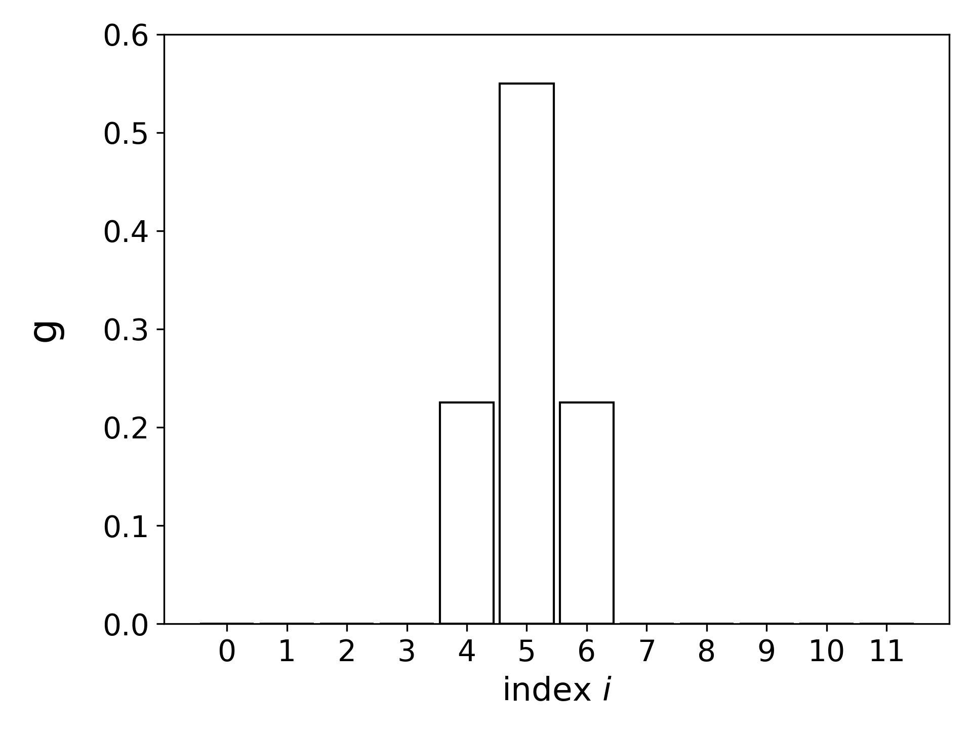
(a)

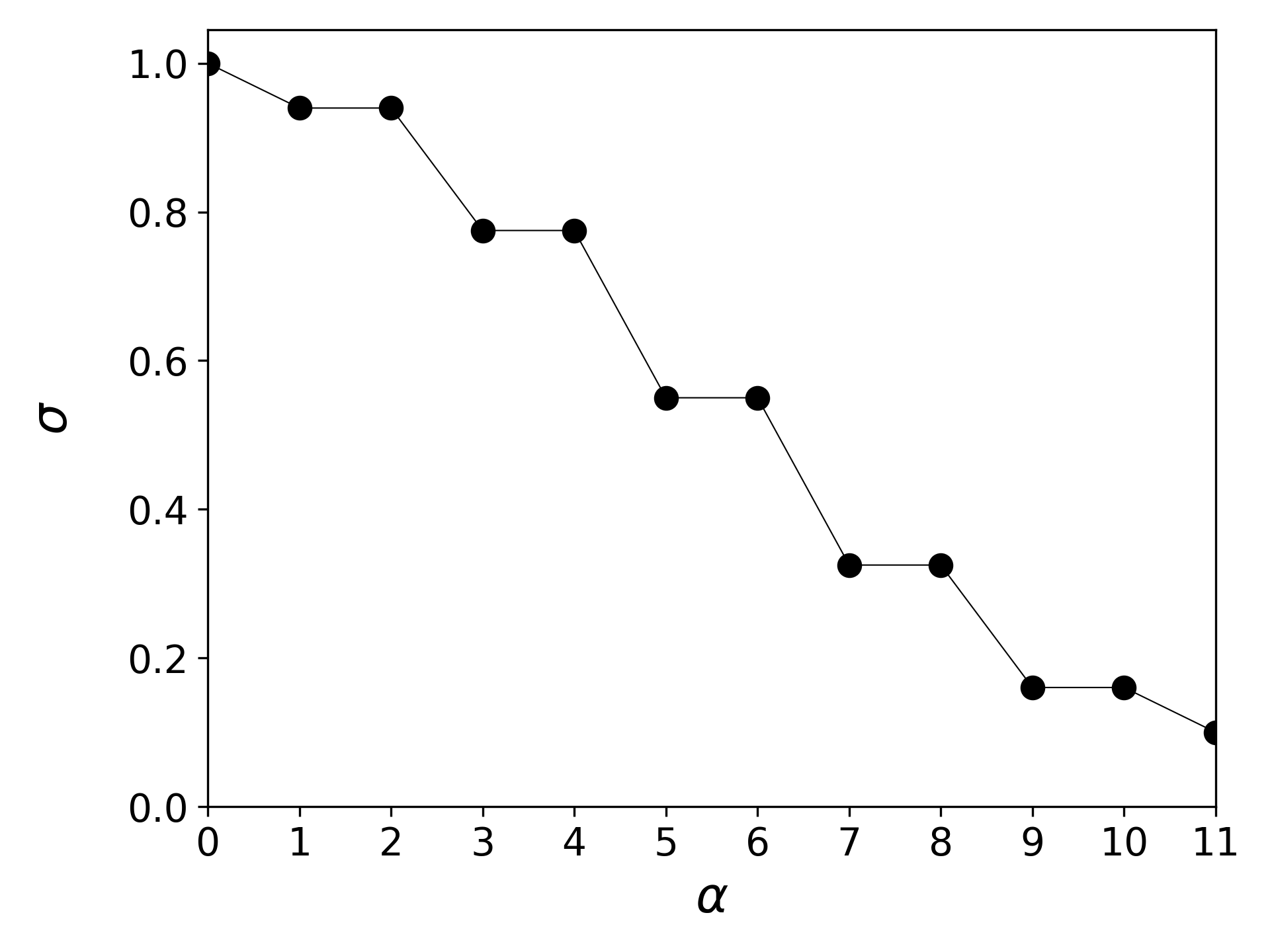
(b)

Figure 1. Illustration of the three-bin blurring function. (a) Image from blurring an original with pixel 5 at 1 and other at 0, for $n=12$. (b) Singular values of the blurring function, ordered by their magnitude. Lines join the values to guide the eye.

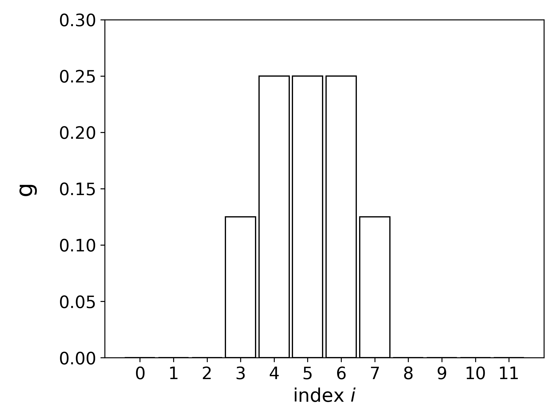
(a)

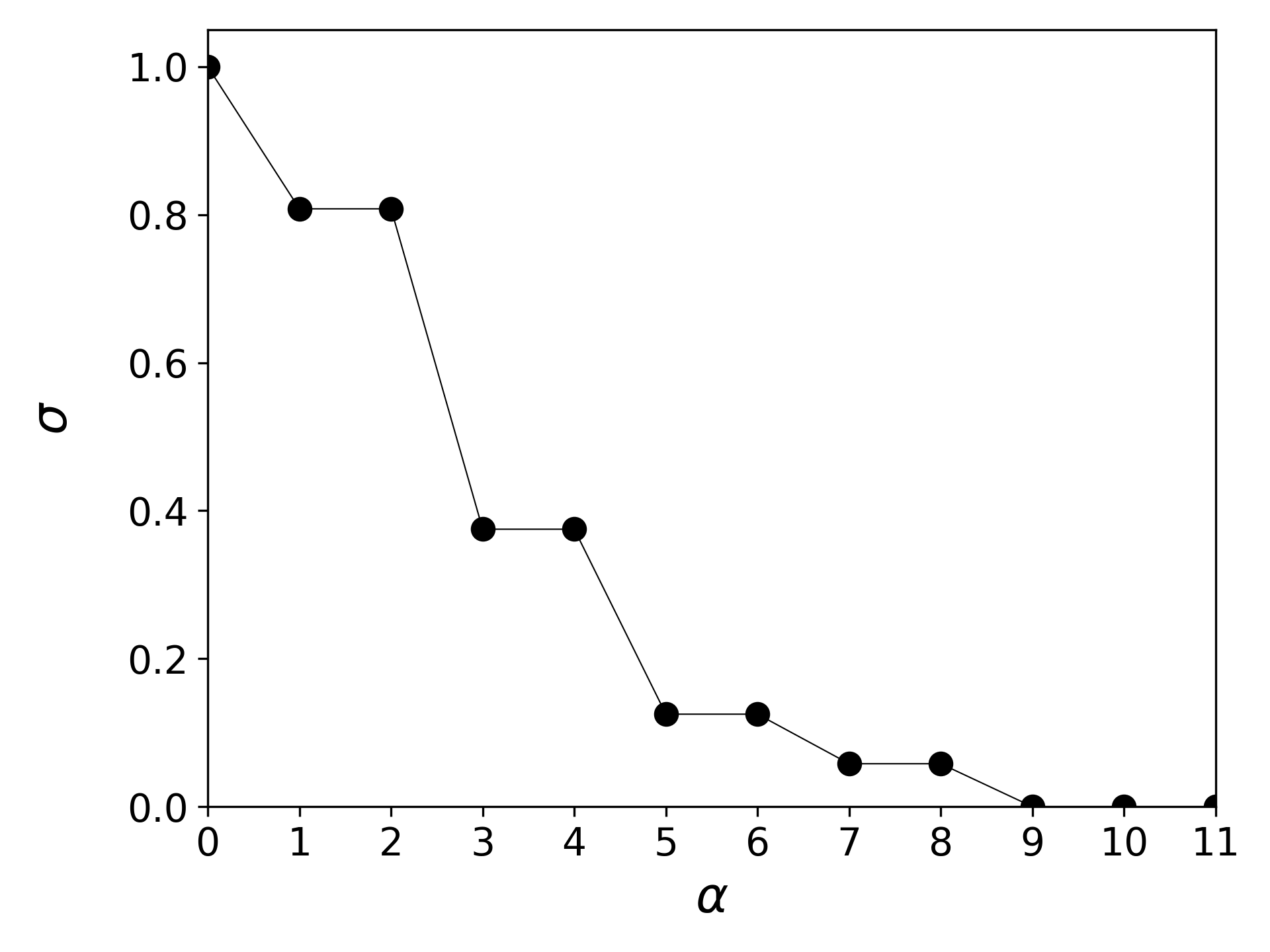
(b)

Figure 2. Illustration of the five-bin blurring function. (a) Image from blurring an original with pixel 5 at 1 and other at 0, for $n=12$. (b) Singular values of the blurring function, ordered by their magnitude. Lines join the values to guide the eye.

Upon applying the transposed blurring matrix to both sides of Eq. (1), we find the norm equation

$$T^{\top}\mathbf{g}=T^{\top}T\,\mathbf{F}\equiv M\mathbf{F}\,.$$ (4)

If we apply SVD to $T$, we get

$$T=\sum_{\alpha=0}^{n-1}\sigma_{\alpha}\,\mathbf{u}_{\alpha}\,\mathbf{v}_{\alpha}^{\top}\,,$$ (5)

where $\mathbf{u}$ and $\mathbf{v}$ are, respectively, the separately orthonormal left and right singular vectors, and we adopt the convention of the singular values $\sigma$ to be nonnegative and ordered in nonincreasing order. Then for the positive definite matrix $M$ we arrive at the following spectral decomposition

$$M=T^{\top}\,T=\sum_{\alpha,\beta}\sigma_{\alpha}\,\sigma_{\beta}\,\mathbf{v}_{\alpha}\,\mathbf{u}_{\alpha}^{\top}\,\mathbf{u}_{\beta}\,\mathbf{v}_{\beta}^{\top}=\sum_{\alpha}\sigma_{\alpha}^{2}\,\mathbf{v}_{\alpha}\,\mathbf{v}_{\alpha}^{\top}\,.$$ (6)

Generally, for original and deblurred images, we shall employ a decomposition in terms of the right singular vectors of the blurring matrix and for the blurred images - in terms of the left:

$$\begin{cases}\mathbf{F}=\sum_{\alpha}F_{\alpha}\,\mathbf{v}_{\alpha}\,,\\ \mathbf{g}=\sum_{\alpha}g_{\alpha}\,\mathbf{u}_{\alpha}\,.\end{cases}$$ (7)

With (1), we then find

$$\mathbf{g}=T\mathbf{F}=\sum_{\alpha}\sigma_{\alpha}\,F_{\alpha}\,\mathbf{u}_{\alpha}\,,$$ (8)

or $g_{\alpha}=\sigma_{\alpha}\,F_{\alpha}$.

The three- and five-bin blurring matrices, Eqs. (2) and (3), which we use here as examples, have some peculiar features. These features may often be encountered in practice, possibly as approximate rather than exact. Thus, these blurring matrices are symmetric, meaning their singular vectors are matrix eigenvectors. Further, with the matrix elements of $T$ depending only on the absolute difference of indices, that dependence extends to the corresponding $M$ matrices. This implies two types of invariance for the matrices $T$ and $M$, impacting the singular vectors. One is the invariance under a shift of matrix indices by some integer. With this, a singular vector, corresponding to some singular value, remains a singular vector, corresponding to the same singular value, after a shift in its indices by an integer. The second invariance is under a reflection of the indices around any chosen index. With this, a singular vector, corresponding to some singular value, remains a singular vector, corresponding to the same singular value, after a reflection of its indices around any chosen index. With these two symmetries, any singular value is at least doubly degenerate unless the corresponding singular vector transforms onto itself, up to a factor of -1, under these transformations.

The spectra of singular values for the two exemplary blurring matrices are shown in Figs. 1(b) and 2(b), and the singular vectors for the five-bin function are shown in Fig. 3. Double degeneracy is seen for most of the singular values. For Fig. 3, we choose the corresponding pairs of singular vectors in the degenerate subspaces so that some symmetry behind the degeneracies is evident, either a reflection or translational one, or both. In each of the spectra, in Figs. 1(b) and 2(b), a nondegenerate singular value of 1 is seen. This value corresponds to the vector that is constant across the pixels. Under blurring, this vector transforms into itself. Also, this vector is invariant under the symmetries. The spectrum of singular values falls off faster for the five- than for the three-bin function, demonstrating a more significant deterioration of the information under the blurring with a broader function. In Fig. 3, it is evident that a faster variation of the vectors over pixels is generally associated with lower singular values. The singular vector with the most rapid variation, alternating between the same positive and negative values from one pixel to another, is invariant under the symmetries. It is the other one that may be nondegenerate. Also, under blurring, it transforms into itself, up to a factor, because it is uniquely alternating and reflection-symmetric about every pixel, which will be preserved by any blurring that depends only on the difference of indices. With a broadening of the blurring function, this vector will likely be the first to be nullified. In Fig. 1(b), the singular value for that vector, with index 11, approaches zero, and the vector is nullified when the blurring matrix evolves into $T_{jj}=0.5$ and $T_{ji}=0.25$, for $j=(i\pm 1)\mod 12$. In Fig. 2(b), the maximally alternating vector is accompanied in the null space by two more vectors, cf., panels (a) and (f) in Fig. 3.

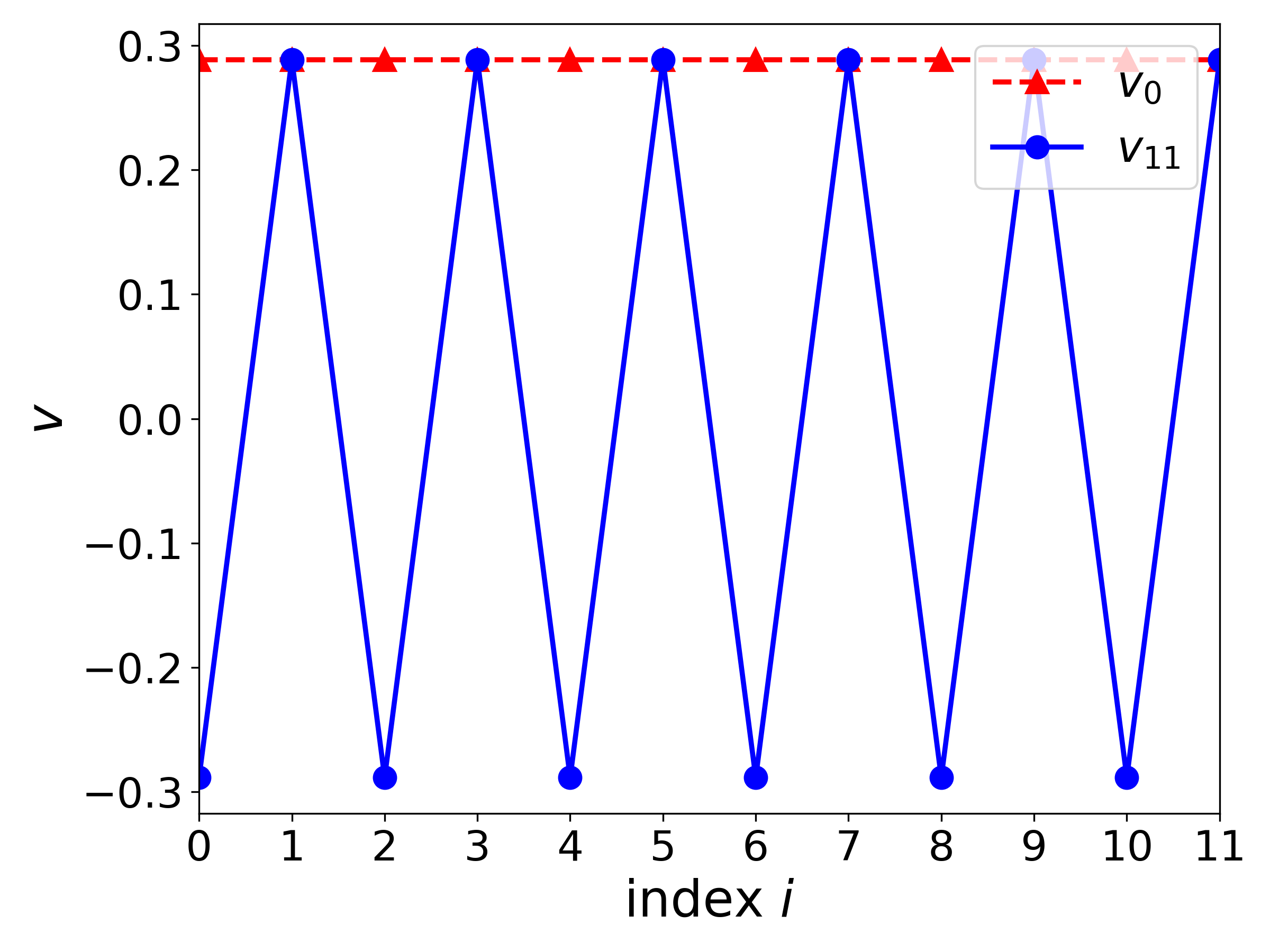
(a)

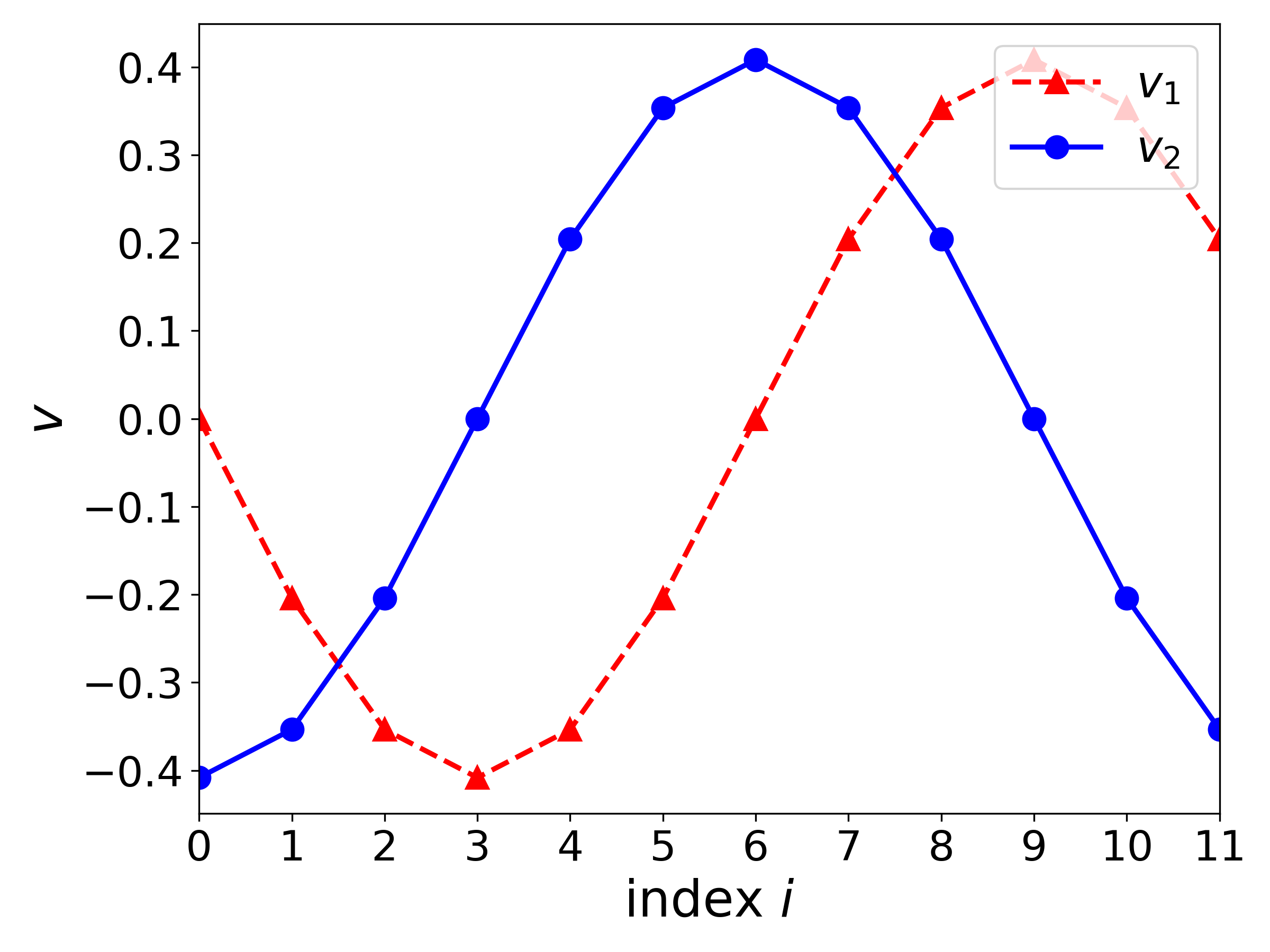
(b)

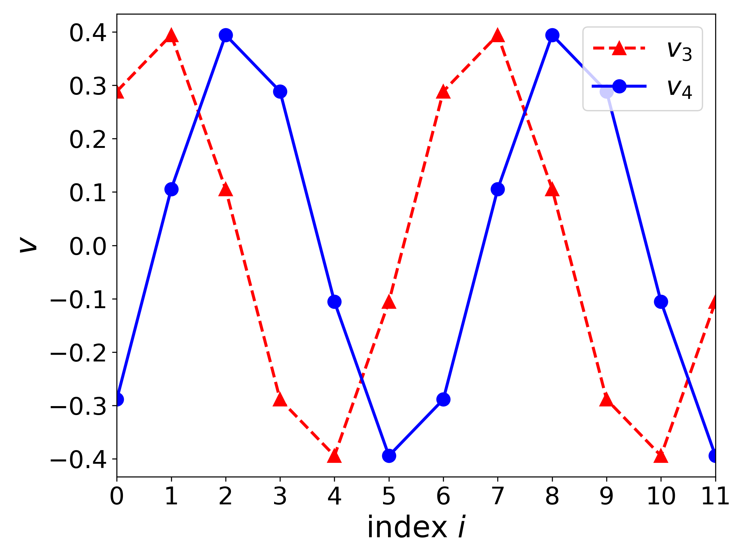
(c)

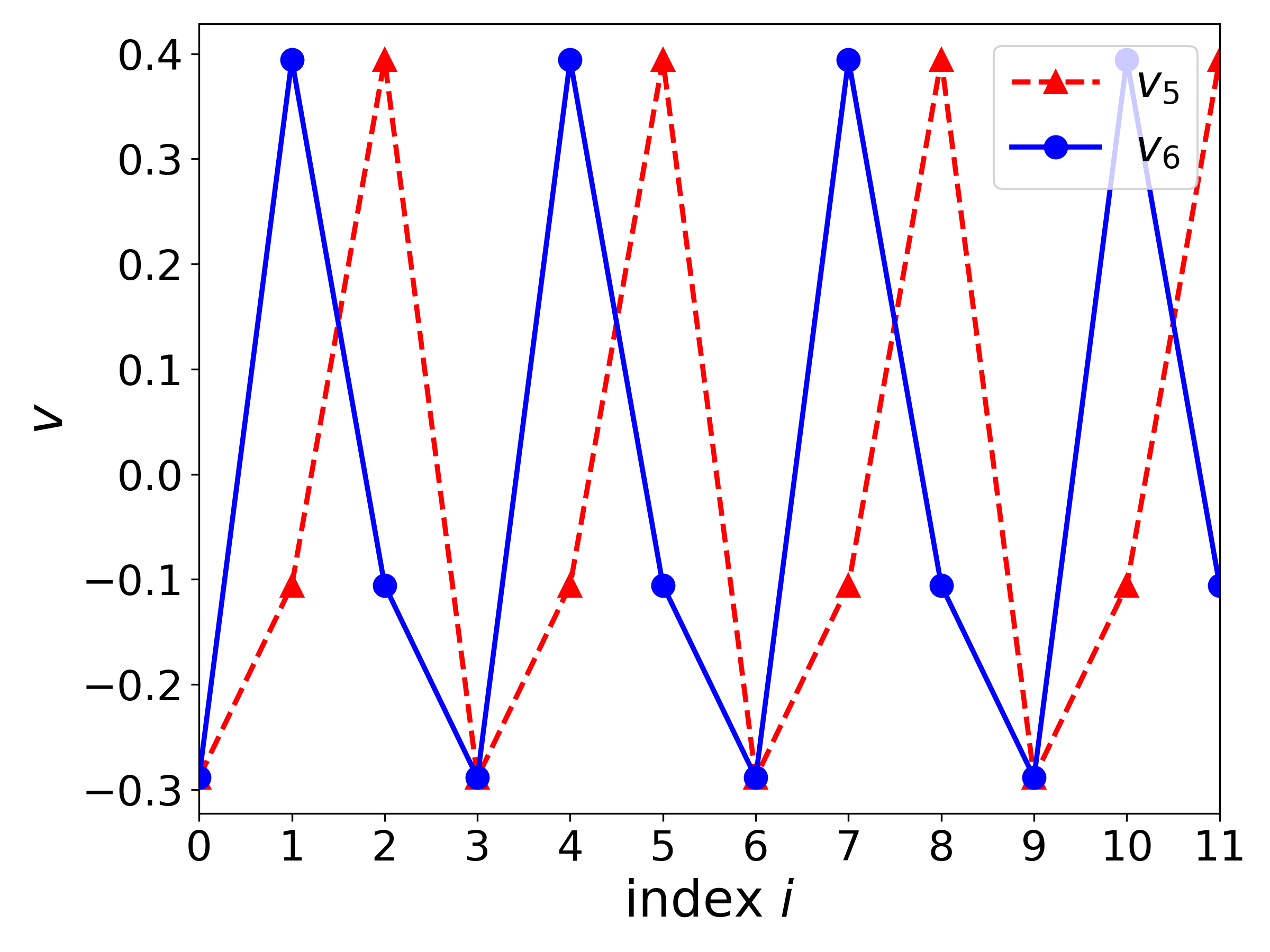
(d)

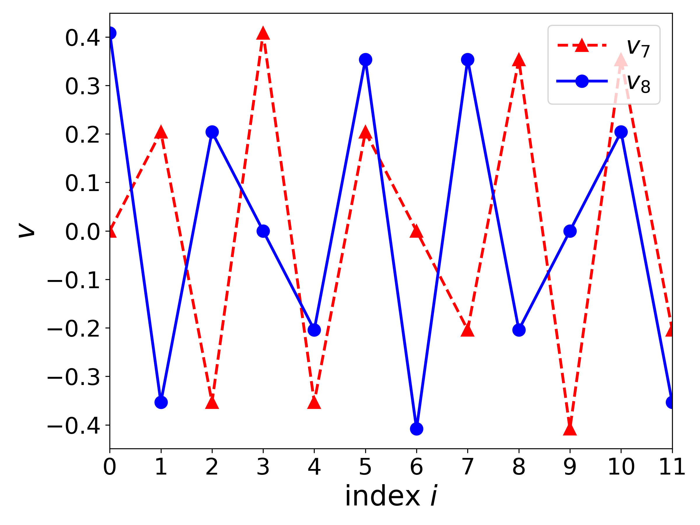
(e)

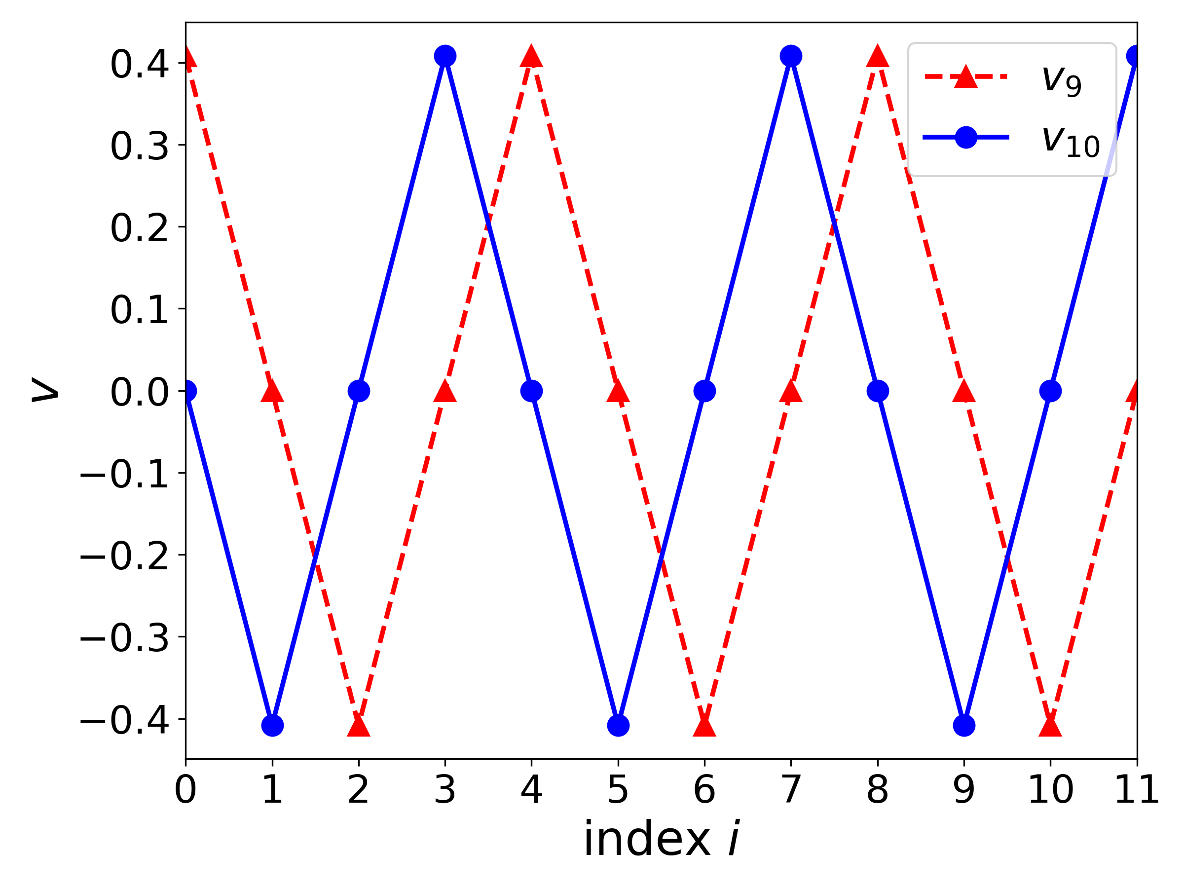
(f)

Figure 3. Singular vectors for the five-bin blurring function. Within degenerate spaces, pairs of vectors are chosen to transform onto the other or itself under reflection and/or translation. Panel (a) shows the two unique vectors that transform onto themselves under the transformations.

3. Deblurring Methods

We next turn to deblurring. We illustrate the deblurring in Fig. 4(a). We take a $\delta$ distribution where only one bin gets intensity 1, and the others get 0. We blur the original image with the 5-bin function (3) and deblur the outcome with the RL method [11, 8], of which the details will be discussed. The blurred and restored images are shown in Fig. 4(a) together with the original. The eye cannot distinguish the RL-restored and original images, thus represented with one set of graphics. In addition, intensity values for the images are shown in Table 1, and within a precision nearing that of the machine we employ, they cannot be distinguished. This may be perceived as astounding, as the singular vectors with the fastest bin-to-bin variation span the null space for the blurring matrix, and they most certainly contribute to the SVD of the $\delta$ distribution.

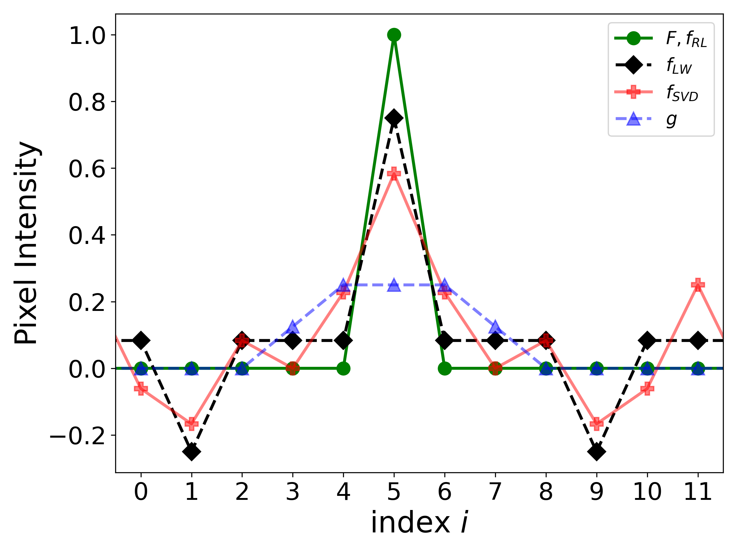
(a)

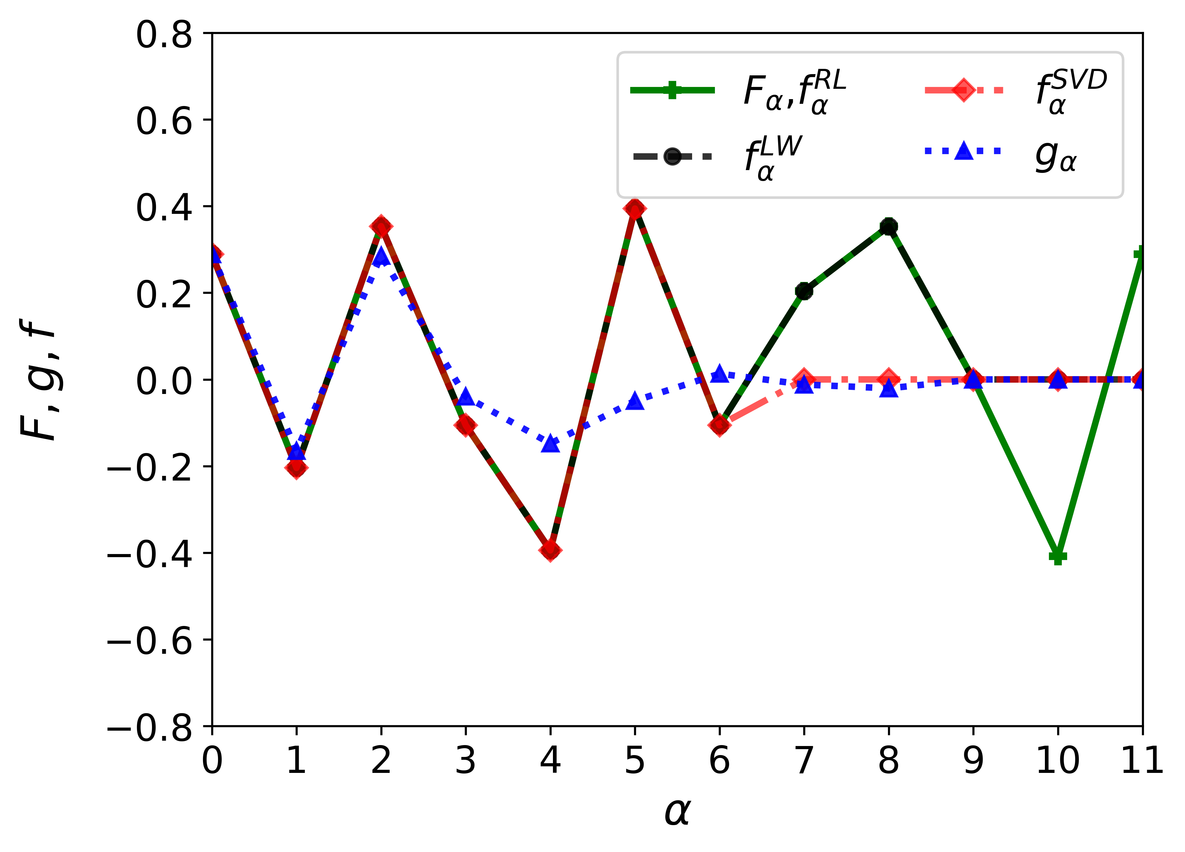
(b)

Figure 4. Deblurring test with a single pixel with index 5 at the intensity 1 and all other pixels at the intensity of 0. (a) The original image $F$ (circles), image $g$ (triangles) from blurring $F$ with the 5-pixel blurring function, and the restored images $f$ from different deblurring methods are displayed. As the image restored following the RL method is not distinguishable by the eye from the original, the circles represent that image, too. The image restored using the LW method is represented by diamonds. Finally, the image that was restored with SVD, where the operational space was reduced ($m=6$ in Eqs. (21) and (22)) compared to LW, is represented by circles. The symbols corresponding to each case are connected with lines. (b) Coefficients of decomposition in the basis of singular vectors vs singular value index for the original and blurred images and images restored with the RL and LW methods.

$i$	$F_{i}$	$g_{i}$	$f_{i}^{RL}$	$f_{i}^{LW}$	$f_{i}^{SVD}$
0	0	0.000	0.000	0.083	-0.061
1	0	0.000	0.000	-0.250	-0.167
2	0	0.000	0.000	0.083	0.083
3	0	0.125	0.000	0.083	0.000
4	0	0.250	0.000	0.083	0.228
5	1	0.250	1.000	0.750	0.583
6	0	0.250	0.000	0.083	0.228
7	0	0.125	0.000	0.083	0.000
8	0	0.000	0.000	0.083	0.083
9	0	0.000	0.000	-0.250	-0.167
10	0	0.000	0.000	0.083	-0.061
11	0	0.000	0.000	0.083	0.250

Table 1. Bin intensities in deblurring the $\delta$-distribution centered at index 5, illustrated in Fig. 4(a). From left to right, the columns represent the bin index ($i$), and then the intensity for the original image ($F_{i}$), for the 5-bin blurred image ($g_{i}$), and the image restored with three different methods: RL ($f_{i}^{RL}$), LW ($f_{i}^{LW}$) and SVD ($f_{i}^{SVD}$).

In the following, we review exemplary deblurring methods within the context of their potential utility in quantitative research analyses. After this section, we shall examine under what circumstances the deblurring can yield faithful results, such as in the example above, and we shall seek conditions and manner under which the deblurring can fail. The iterative methods aim to restore a blurred image to its original form by iteratively improving the estimate of the blur-free image. These methods take as input some initial guess of the blur-free image, the blurring matrix, and a criterion for the number of iterations to be carried out. The typical initial guesses are the uniform image or the blurred image. As the blur-free image is to improve with each iteration, naively, a more accurate output is to be obtained with more iterations - in practice, this may not be the case.

We use below $k$ as an iteration index while discussing the iterative methods.

3.1. Richardson-Lucy method, classical and regularized

The classical RL algorithm iteratively upgrades the restored image $f$, given the blurred image $g$, according to [11, 8, 3]

$$f_{i}^{(k+1)}=A_{i}^{(k)}\,f_{i}^{(k)}\,.$$ (9)

Here, the amplification factor $A_{i}$ for the $i$’th pixel intensity is

$$A_{i}^{(k)}=\frac{1}{q_{i}}\sum_{j}T_{ji}\frac{g_{j}}{g_{j}^{(k)}}\,,$$ (10)

$i,j,m=0,1,2,\ldots,n-1$, $g_{j}^{(k)}=\sum_{m}T_{jm}f_{m}^{(k)}$ is the blurred-image prediction for the restored image $f^{(k)}$ at the $k$’th step of restoration, $T$ is the before introduced point spread function or blurring matrix, and $q_{i}=\sum_{j}T_{ji}$ serves the normalization. The normalization factors for the introduced blurring-function examples are unity, $q_{i}\equiv 1$.

The regularized RL algorithm modifies the iteration equation to

$$f_{i}^{(k+1)}=A_{i}^{(k)}\,I^{k}_{i}\,f_{i}^{(k)}\quad i,j,m=0,1,2,\ldots,n-1\,,$$ (11)

where the regularization factor is [4, 3]

$$\begin{split}I^{(k)}_{i}&=\frac{1}{1-\Lambda\operatorname{div}\left(\frac{\nabla f_{i}^{(k)}}{|\nabla f_{i}^{(k)}|}\right)}\\ &=\begin{cases}\frac{1}{1-\Lambda}\,,&\text{ if }f^{(k)}_{i}<f^{(k)}_{[(i-1)\,\mathrm{mod}\,n],\,[(i+1)\,\mathrm{mod}\,n]}\,,\\ \frac{1}{1+\Lambda}\,,&\text{ if }f^{(k)}_{i}>f^{(k)}_{[(i-1)\,\mathrm{mod}\,n],\,[(i+1)\mathrm{mod}\,n]}\,,\\ 1\,,&\text{ }\text{ otherwise }\,.\end{cases}\end{split}$$ (12)

for $i=0,1,2,\ldots,n-1$. Here, the r.h.s. is the one-dimensional version [3] of the center expression [4] in which $\nabla$ is the gradient and $|\nabla f_{i}^{(k)}|$ is $\ell_{1}$-norm; $\Lambda$ is a small positive regularization coefficient. The role of the regularization factor is the suppression of uncontrolled rise, during iterations, of contributions to the restored image from the fastest varying singular vectors corresponding to vanishing or minimal singular values. The typical signature of such an uncontrolled rise is developing a bin-to-bin sea-saw pattern in the restored image. As SVD might not be applied in parallel to the RL-restoration and the direct connection of the regularization factor $I$ to SVD is not obvious, it is common to make $\Lambda$ small enough that no pathological signs in the restored image appear.

The restoration of the $\delta$-distribution of Fig. 4(a) with the RL method, from the blurred image there, with or without regularization, yields a result that is not distinguishable by eye from the original, so they share the graphical representation in the figure. The numerical values for the restoration are provided in Table 1. Another test to which we subject the deblurring methods is presented in Fig. 5. The original image $F$ is a ramp with pixels 5-8 at intensity 1 and other pixels at intensity 0. The blurring, yielding $g$, is performed with the 5-bin blurring function. The results of RL deblurring, without or with regularization, are not distinguishable by eye from the original, but so are the results of deblurring with other methods that we will discuss next. The numerical values from the ramp tests can be found in Table 2.

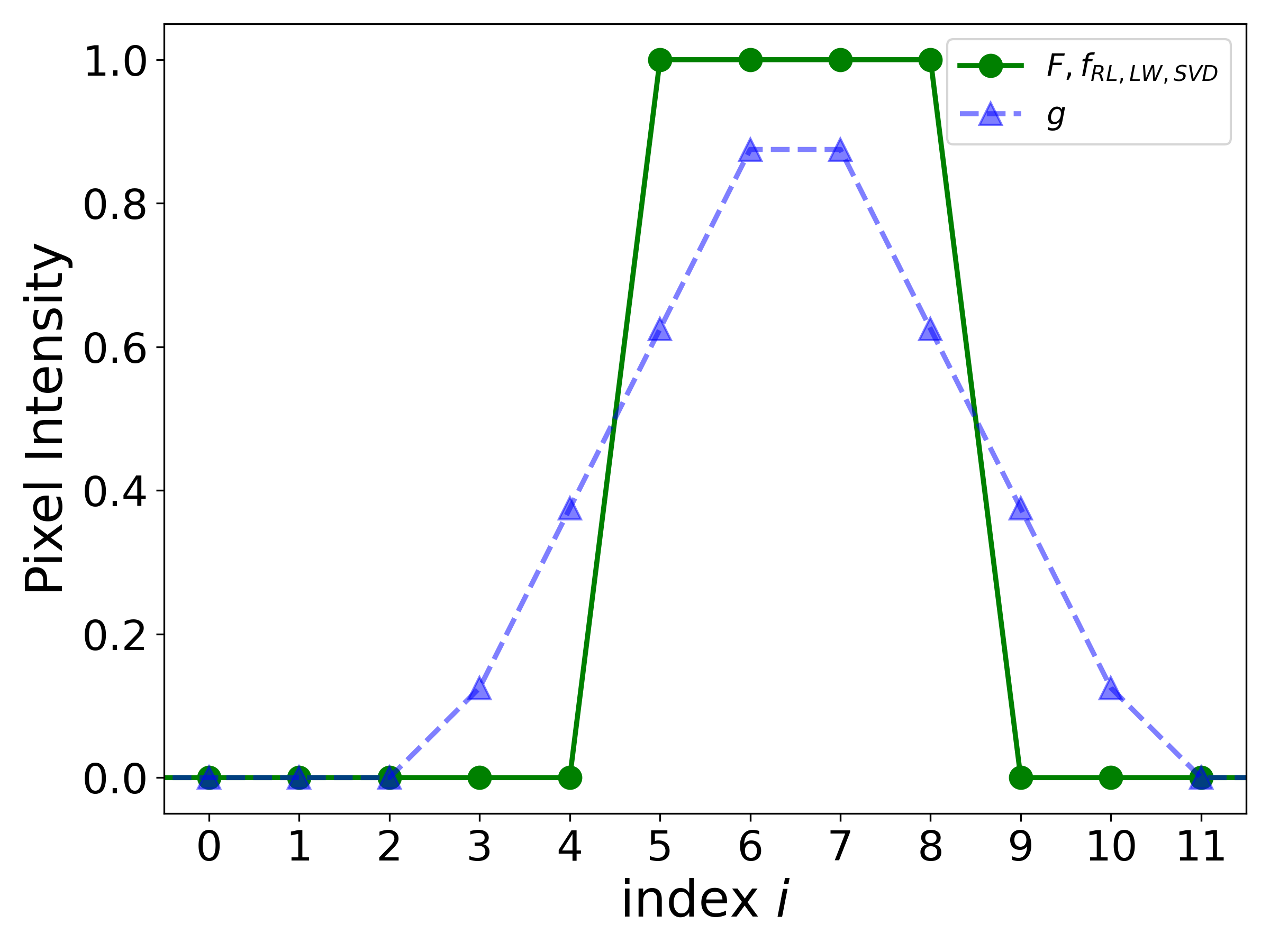
Figure 5. Deblurring test with a 4-pixel ramp. In the original image, the intensity is 1 for the pixels 5-8 and 0 for the others. The operational space for SVD is here the full row space of $T$.

$i$	$F_{i}$	$g_{i}$	$f_{i}^{RL}$	$f_{i}^{LW}$	$f_{i}^{SVD}$
0	0	0.000	0.000	0.000	0.000
1	0	0.000	0.000	0.000	0.000
2	0	0.000	0.000	0.000	0.000
3	0	0.125	0.000	0.000	0.000
4	0	0.375	0.000	0.000	0.000
5	1	0.625	1.000	1.000	1.000
6	1	0.875	1.000	1.000	1.000
7	1	0.875	1.000	1.000	1.000
8	1	0.625	1.000	1.000	1.000
9	0	0.375	0.000	0.000	0.000
10	0	0.125	0.000	0.000	0.000
11	0	0.000	0.000	0.000	0.000

Table 2. The numerical values from the 4-pixel ramp deblurring test, with the RL, SVD, and LW methods, illustrated in Fig. 5.

3.2. Landweber Method

The Landweber (LW) method [7] can be viewed as the steepest-descent method for minimizing the square deviation between the brightness distribution for the generated and blurred images,

$$\left\|\mathbf{g}-T\mathbf{f}\right\|^{2}_{2}\,.$$ (13)

Iterative adjustments in $\mathbf{f}$ take the form

$$\mathbf{f}^{(k+1)}=\mathbf{f}^{(k)}+\beta T^{T}(\mathbf{g}-T\mathbf{f}^{(k)})\,,$$ (14)

where $0<\beta<2/\|T^{T}T\|$ for convergence. With the $T$ multiplication in (14), it is apparent that the iterations do not change the null-space content in $f$. The null-space content may be suppressed completely in $f$ by replacing the minimized quantity (13) with

$$\left\|\mathbf{g}-T\mathbf{f}\right\|^{2}_{2}+\epsilon\left\|\mathbf{f}\right\|^{2}_{2}\,,$$ (15)

where $0<\epsilon\ll(\sigma_{\alpha})_{min}^{2}$ and $(\sigma_{\alpha})_{min}$ is the smallest singular value of which the contribution to $f$ should not be disturbed. The iterations are then modified to

$$\mathbf{f}^{(k+1)}=(1-\beta\epsilon)\mathbf{f}^{(k)}+\beta T^{T}(\mathbf{g}-T\mathbf{f}^{(k)})\,.$$ (16)

The results from the deblurring of the blurred $\delta$-distribution with the LW method are provided in Fig. 4 and Table 1. The corresponding results from processing the 4-pixel ramp are provided in Fig. 5 and Table 2. While the LW method struggles to restore the $\delta$ distribution, yielding, in particular, negative intensity values, it faithfully restores the 4-pixel ramp. This may be surprising, and we will return to this issue later in this Section.

3.3. Deblurring Using Singular Value Decomposition

The deblurring can be further carried out by employing SVD explicitly. In general, the SVD deblurring [5, 15, 10] seeks the best approximation to the blurred image in a reduced subspace of singular vectors, which in particular should exclude the null space for $T$, minimizing the square deviation

$$\left\|\mathbf{g}-T_{m}\mathbf{f}\right\|^{2}_{2}\,,$$ (17)

where

$$T_{m}=\sum_{\alpha=0}^{m-1}\sigma_{\alpha}\,\mathbf{u}_{\alpha}\,\mathbf{v}_{\alpha}^{\top}\,,$$ (18)

and $m\leq n$. The minimization of (17) is equivalent to the minimization of the square deviation within the reduced subspace only

$$\left\|\mathbf{g}_{m}-T_{m}\mathbf{f}\right\|^{2}_{2}\,,$$ (19)

where

$$\mathbf{g}_{m}=\sum_{\alpha=0}^{m-1}g_{\alpha}\,\mathbf{u}_{\alpha}\,,$$ (20)

with the minimum reached for

$$f_{\alpha}=\frac{g_{\alpha}}{\sigma_{\alpha}}\,,\hskip 20.00003pt\text{for}\hskip 5.0pt\alpha<m\,.$$ (21)

Outside of the considered subspace, the expansion coefficients for $\mathbf{f}$ are set to zero,

$$f_{\alpha}=0\,,\hskip 20.00003pt\text{for}\hskip 5.0ptm\leq\alpha<n\,.$$ (22)

In the tests of this Section, the SVD method yields the same results as LW when its operational space is maximal, i.e., identical to the row space of the blurring matrix $T$. Regarding the 4-pixel ramp test with results in Fig. 5 and Table 2, we keep the operational space for SVD maximal. However, in the $\delta$-function test with results in Fig. 4 and Table 1, we reduce the operational space for SVD to $m=6$, see Fig. 3 for the corresponding singular vectors. With the reduction, the quality of the restoration significantly deteriorates. The location and strength of negative intensities in the restored image are similar for $m=8$ (identical to LW within precision) and $m=6$, cf. Eqs. (21) and (22).

3.4. Methods’ Assessment

We call the original images, such as in Figs. 4(a) and 5, where a substantial fraction of the pixels has an intensity zero or low compared to the maximal, as having high contrast. When such images are moderately blurred, the deblurring methods with the nonnegativity constraint for intensity built into the deblurring process, such as RL, generally perform far better than methods that lack the constraint, such as LW or SVD, see the case of the $\delta$-distribution of Fig. 4(a). In this case, the two latter methods yield negative intensity values in the restored images. Amazingly, while the $\delta$-distribution contains contributions from the $v_{10}$ and $v_{11}$ vectors in the null space, the nonnegativity constraint allows the RL method to restore their contributions faithfully despite their singular values being zero, see Fig. 4(b). Without the nonnegativity constraint, the content of the null space, in the case of LW, or excluded space, in the case of SVD, stays at zero.

One puzzling outcome of the tests so far is that the LW method and the SVD method, when its excluded space is identical to the null space, perform as well as RL in restoring the 4-pixel ramp in Fig. 5, even though they struggle with the $\delta$-distribution. The mystery is solved when looking at the null-space singular vectors in Fig. 3 and the original ramp in Fig. 5: a ramp with an even number of pixels at the same intensity lacks any null-space contribution for our blurring function of Eq. (3). When the ramp’s extension is changed to an odd number of pixels or the ramp is sloped, the LW and SVD methods can develop negative intensity values for the restored image, just like in the case of the $\delta$ distribution.

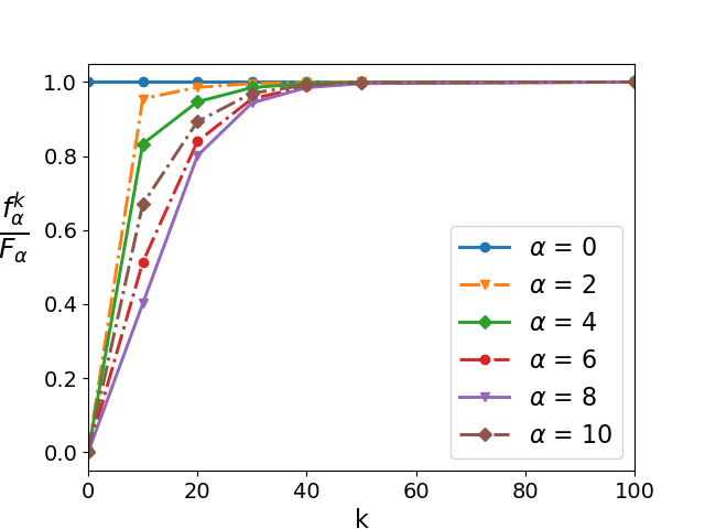
(a)

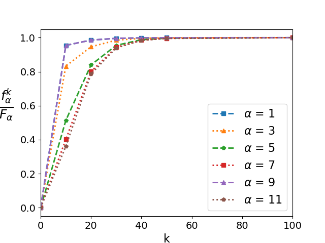
(b)

Figure 6. Restored-image expansion coefficients in singular vectors, as a function of the RL iteration step $k$, normalized to the coefficients for the original $\delta$-distribution image, for even-index (a) and odd-index (b) singular vectors.

Given the benefits of the built-in nonnegativity constraint, we will further exclusively rely on the RL deblurring method. Other methods may perform similarly when supplemented with this type of constraint. In employing the RL method, the iteration progress is sometimes used as a tool. Figure 6 shows how the expansion coefficients in singular vectors for the restored image behave as a function of the RL iteration step. Here, the original image is the $\delta$-distribution, and the starting image is the uniform distribution. One can observe that the higher the index of the singular vector, the generally slower the approach of the coefficient to its asymptotic value. This can be understood in terms of the weakening impact of expansion coefficients on the amplification factors (10) when the singular value decreases, as

$$\frac{\text{d}A_{i}^{(k)}}{\text{d}f_{\alpha}^{(k)}}\propto\sigma_{\alpha}\,,$$ (23)

for $g_{i}>0$. Null-space and low singular-value coefficients will be impacted by the positivity constraint and/or regularization, and in Fig. 6, we can see their pace of approach to the asymptotic values to be lumped.

4. Exploring the limits of deblurring

In the context of the deblurring applications in quantitative research in nuclear and particle physics, it is important to understand when and how the deblurring can falsify the results. We have observed the role that positive definiteness could play in restoring the null-space contributions to a distribution. However, intuitively, one could expect the positive definiteness to play a little role when the original distribution is uniformly far from zero on the general distribution’s variation scale. Below, we will compare the performance of the classic RL method in those different situations. In cases when there is no positive definiteness that one can fall on, the regularization can help improve the performance of a deblurring method. However, the regularization must be a compromise with some adverse effects, too, as may be evident from Eq. (15).

4.1. High vs Low Contrast

For high-contrast original images, such as in Fig. 4(a) and 5, we have observed that the deblurring with the nonnegativity constraint can restore the null-space components from the blurred images. Notably, for the nonnegativity constraint to be impactful, the number of pixels at low intensity compared to the rest must be comparable to the dimension of the null space. We now confront that situation to one for low-contrast original images where the intensity for most pixels varies within a small range relative to the maximal intensity.

An exemplary low-contrast case of a $\delta$-function superimposed on a high uniform background is illustrated in Fig. 7(a). When the classical RL method is applied to the blurred image, the method fails, on the scale of the $\delta$-function norm, in a similar manner as the methods without the nonnegativity constraint in the high-contrast case of Fig. 4(a). Again, we start the RL iterations in this illustration with a uniform image. Though the nonnegativity is there for the RL method, it does not impact restoration when the background is sufficiently elevated. Fig. 7(b) complements the results of (a) with coefficients of decomposition in the basis of singular vectors, demonstrating that the coefficients for the null space are not restored for the classical RL method, unlike in Fig. 4(b). For impactful constraints, we turn to the regularized RL method, where restoration is modified compared to the classical method depending on the differences in the intensity of adjacent pixels, suppressing local extrema. With a low $\Lambda=0.0001$, the original image is satisfactorily restored in Fig. 7(a).

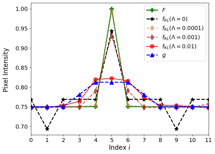
(a)

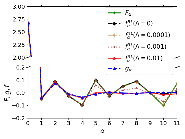
(b)

Figure 7. Deblurring test with a single pixel with index 5 at intensity elevated by 0.25 over a high uniform background at 0.75. (a) Crosses represent the original image $F$ and triangles - the image $g$ from blurring $F$ with the 5-pixel blurring function. Moreover, the restored images $f$ from different versions of the RL method are displayed. Circles represent the image restored using the classical RL method. Diamonds, wide and slim, and stars represent the images restored with the regularized RL method at, respectively, $\Lambda=0.001$, 0.001, and 0.01. The symbols corresponding to each case are connected with lines. (b) Coefficients of decomposition in the basis of singular vectors for the cases in (a) vs singular-value index.

Additional examples of restoration of images at different contrast levels are shown in Fig. 8.

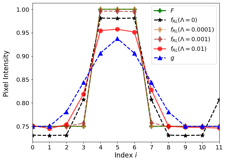
(a)

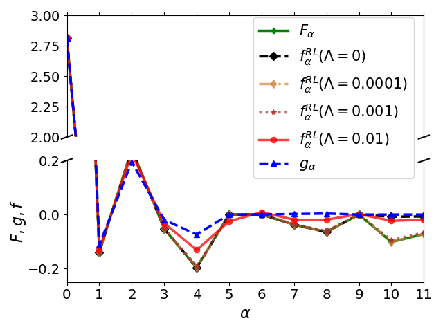
(b)

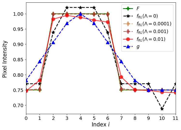
(c)

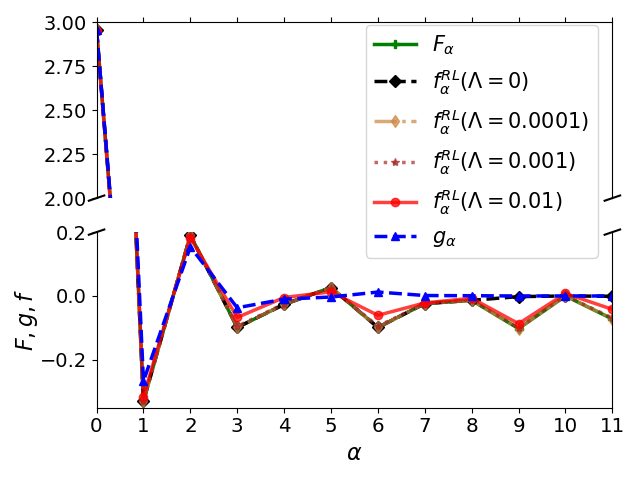
(d)

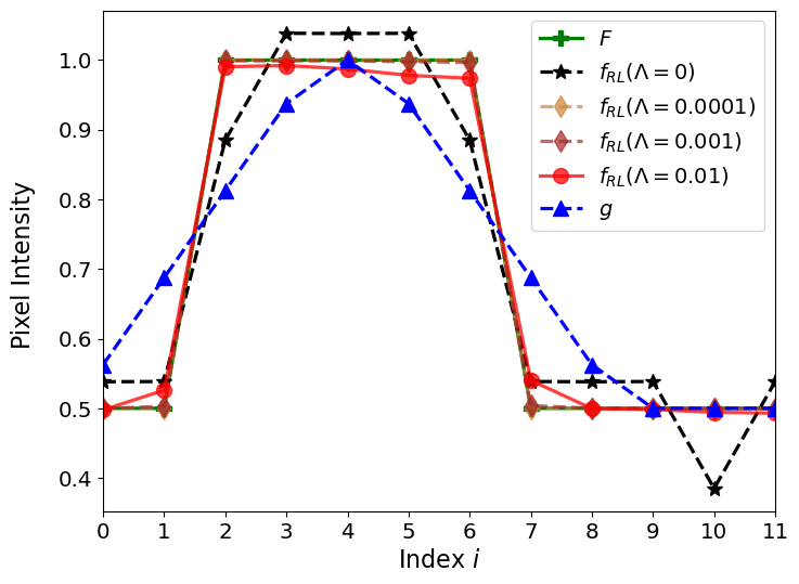
(e)

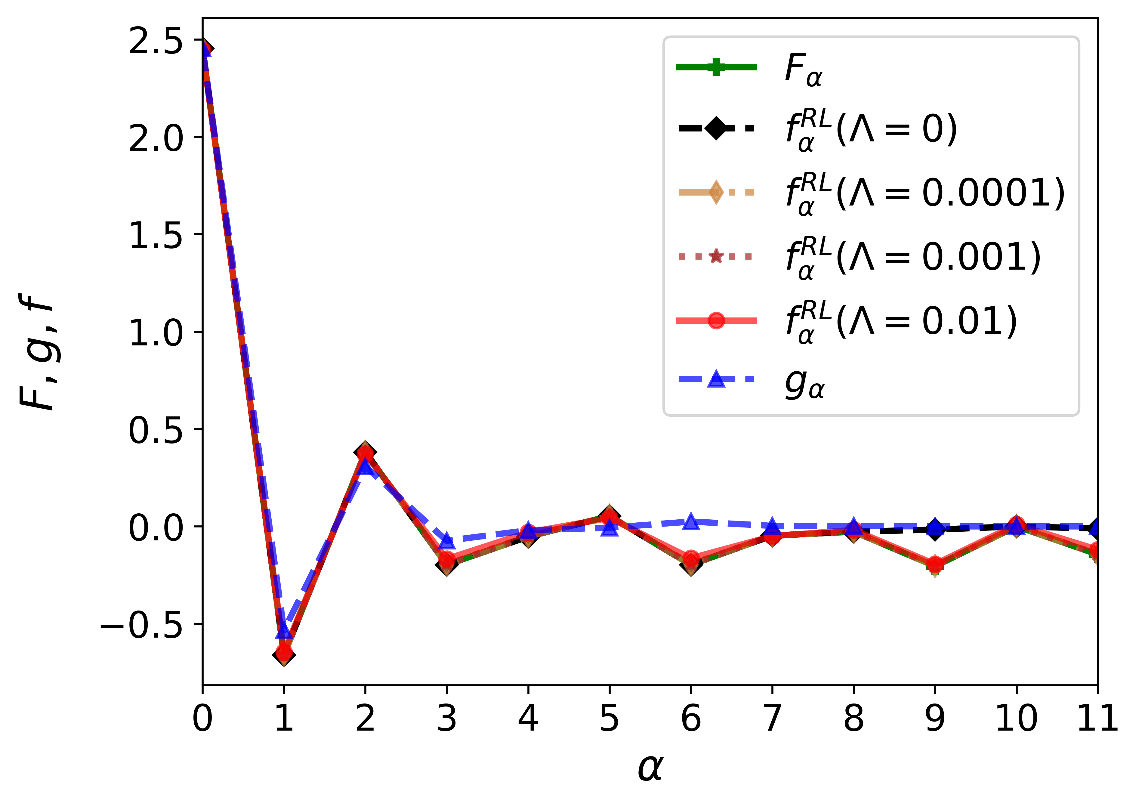
(f)

Figure 8. Deblurring tests such as in Fig. 7 for other exemplary low-contrast images, with matching information for each of these presented in panels (a) and (b), (c) and (d), and (e) and (f), respectively.

4.2. Impact of Initialization

For a low-contrast original image $F$, it is possible to add a significant null-space component to that image, without violating intensity nonnegativity. When such a combination is fed to the classical RL method as the starting guess $f^{(0)}$, mathematically, the restoration iterations will never suppress the added spurious null-space component, yielding that starting guess as the fully restored image $f$. Even added components out of low-singular-value vectors may be only slowly modified in iterations.

To get around excessive spurious null-space or low-singular value admixtures to the restored image, it helps to start the classical RL iterations with an image that lacks such components, such as the uniform image. In Fig. 9, we show what happens within the classical RL restoration when the restoration of a low-contrast image is started with a significant null-space component in the first guess for the image instead of the uniform guess. The null-space component’s strength persists for $\Lambda=0$ at significant strength in the limit of many restoration steps. Notably, the null-space components are not likely to adjust to the values for the original image in the absence of an impact of the nonnegativity constraint, no matter how the iterations are started, including with the uniform image. In Figs. 7 and 8, we can see that classical restorations of low-contrast images started with uniform guesses, tend to underestimate the magnitude of the null-space components in the restored images. In particular, the panels (a) and (b) in Fig. 8 are analogous to Fig. 9 but differ importantly in initialization. As may be seen in Figs. 7, 8, and 9, the null-space components get under some control after the regularization is switched on.

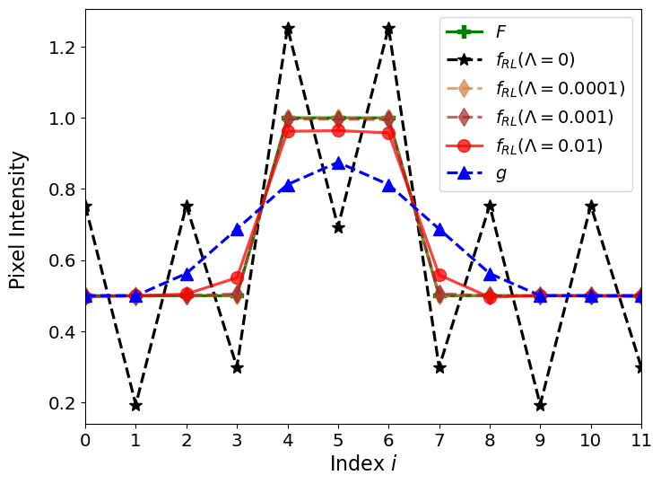
(a)

(b)

Figure 9. Sensitivity of an RL restoration to null-space content at iteration start and to the regularization strength. The RL iterations here are started with the original image with an $\alpha=11$ component added. The classical RL method ($\Lambda=0$) leaves the null-space content intact. An RL method with regularization ($\Lambda>0$) suppresses the superimposed spurious null-space content, but excessive regularization strength, such as for $\Lambda=0.01$, can chip off the null-space content in the restored image compared to the original.

4.3. Impact of Regularization

In examining the cases of restoration of interesting original images with few significant intensity jumps in Figs. 7 and 8, we can see that the regularization can dramatically improve image restoration. The particular regularization of Eqs. (11) and (12) biases against multiple pronounced extrema and, with that, suppresses significant spurious null-space contributions that could be added to the restored low-contrast image for the classical RL method.

While a modest regularization within the RL method can help restore the null-space content of the original image, an excessive regularization can act to suppress not only that content but also contributions from singular vectors corresponding to low nonzero singular values. This is illustrated in Figs. 7 and 8, which include results from RL restorations with progressively strengthening regularization. We can see that with the progressing strength of regularization, the features of the restored images begin to evolve away from the original image toward the blurred image. In a sense, the regularization needed for low-contrast images amounts to trading stronger blurring for weaker.

5. Summary

We have examined the iterative RL deblurring method and partially other methods in the context of the utility of deblurring in nuclear and high-energy physics. We disregarded explicit noise in the images for the time. SVD of the blurring matrix is an essential tool in understanding both the blurring and deblurring processes. For decreasing singular values, the singular vectors generally exhibit faster variation with pixel position. Symmetries of the blurring matrix generally give rise to symmetries of the singular vectors and may make the left- and right-hand vectors coincide. Blurring strength may be characterized by the falloff of singular values with a singular-vector index. A strong enough blurring can give rise to a null space in the SVD. A model one-dimensional system of 12 pixels with a periodic boundary condition has served to illustrate our points. For high-contrast images, where the number of pixels at zero or near-zero intensity, compared to maximal in the image, is comparable to the null-space dimension, the nonnegativity constraint built into a deblurring can help restore the null-space content in the processed image. For lower-contrast images, a regularization acting against multiple extrema in the restored image helps control the null-space content. However, a too-strong regularization may start affecting the restored image like the blurring one tries to correct.

Received xxxx 20xx; revised xxxx 20xx; early access xxxx 20xx.

References

- [1] J. Biemond, R.L. Lagendijk and R.M. Mersereau “Iterative methods for image deblurring” Conference Name: Proceedings of the IEEE In Proc. IEEE 78.5, 1990, pp. 856–883 DOI: 10.1109/5.53403
- [2] G. D’Agostini “A multidimensional unfolding method based on Bayes’ theorem” In Nucl. Instrum. Methods Phys. Res. A 362.2, 1995, pp. 487–498 DOI: 10.1016/0168-9002(95)00274-X
- [3] Pawel Danielewicz and Mizuki Kurata-Nishimura “Deblurring for nuclei: 3D characteristics of heavy-ion collisions” Publisher: American Physical Society In Phys. Rev. C 105.3, 2022, pp. 034608 DOI: 10.1103/PhysRevC.105.034608
- [4] Nicolas Dey et al. “Richardson–Lucy algorithm with total variation regularization for 3D confocal microscope deconvolution” _eprint: https://analyticalsciencejournals.onlinelibrary.wiley.com/doi/pdf/10.1002/jemt.20294 In Microsc. Res. Tech. 69.4, 2006, pp. 260–266 DOI: https://doi.org/10.1002/jemt.20294
- [5] Per Christian Hansen, James G. Nagy and Dianne P. O’Leary “Deblurring Images”, Fundamentals of Algorithms Society for IndustrialApplied Mathematics, 2006 URL: https://epubs.siam.org/doi/book/10.1137/1.9780898718874
- [6] M.. Khan “Iterative Methods of Richardson-Lucy-Type for Image Deblurring” In NMTMA 6.1, 2013, pp. 262–275 DOI: 10.4208/nmtma.2013.mssvm14
- [7] L. Landweber “An Iteration Formula for Fredholm Integral Equations of the First Kind” Publisher: Johns Hopkins University Press In Am. J. Math. 73.3, 1951, pp. 615–624 DOI: 10.2307/2372313
- [8] L.. Lucy “An iterative technique for the rectification of observed distributions” In Astron. J. 79, 1974, pp. 745 DOI: 10.1086/111605
- [9] Pierre Nzabahimana et al. “Deconvoluting experimental decay energy spectra: The 26O case” Publisher: American Physical Society In Phys. Rev. C 107.6, 2023, pp. 064315 DOI: 10.1103/PhysRevC.107.064315
- [10] Lothar Reichel “Introduction to Numerical Computing I. Lecture Notes”, 2013 URL: https://www.math.kent.edu/~reichel/courses/intr.num.comp.1/syllabus.html
- [11] William Hadley Richardson “Bayesian-Based Iterative Method of Image Restoration” Publisher: Optical Society of America In J. Opt. Soc. Am., JOSA 62.1, 1972, pp. 55–59 DOI: 10.1364/JOSA.62.000055
- [12] Fagun Vankawala, Amit Ganatra and Amit Patel “A Survey on Different Image Deblurring Techniques” Publisher: Foundation of Computer Science (FCS) In Int. J. Comput. Appl. 116.13, 2015, pp. 15–18 URL: https://www.ijcaonline.org/archives/volume116/number13/20396-2697
- [13] J. Vargas, J. Benlliure and M. Caamaño “Unfolding the response of a zero-degree magnetic spectrometer from measurements of the resonance” In Nucl. Instrum. Methods Phys. Res. A 707, 2013, pp. 16–25 DOI: 10.1016/j.nima.2012.12.087
- [14] JunHuai Xu et al. “Reconstruction of Bremsstrahlung -rays Spectrum in Heavy Ion Reactions with Richardson-Lucy Algorithm” arXiv, 2024 DOI: 10.48550/arXiv.2405.06711
- [15] Christian D. Zuninga “Singular Value Decomposition for Imaging Applications” SPIE, 2021 URL: https://spie.org/Publications/Book/2611523