Error Inhibiting Methods for Finite Elements

Abstract

Finite Difference methods (FD) are one of the oldest and simplest methods for solving partial differential equations (PDE). Block Finite Difference methods (BFD) are FD methods in which the domain is divided into blocks, or cells, containing two or more grid points, with a different scheme used for each grid point, unlike the standard FD method.

It was shown in [5] and [6] that BFD schemes might be one to three orders more accurate than their truncation errors. Due to these schemes’ ability to inhibit the accumulation of truncation errors, these methods were called Error Inhibiting Schemes (EIS).

This manuscript shows that our BFD schemes can be viewed as a particular type of Discontinuous Galerkin (DG) method. Then, we prove the BFD scheme’s stability using the standard DG procedure while using a Fourier-like analysis to establish its optimal convergence rate.

We present numerical examples in one and two dimensions to demonstrate the efficacy of these schemes.

1 Introduction

This manuscript is concerned with numerical solutions to the Heat equation:

$$\dfrac{\partial u({{\bf x}},t)}{\partial t} = \nabla^{2}u({{\bf x}},t)\;,\qquad x\in\Omega\subset{\mathbb{R}}^{d}\mbox{ , }t\geq 0$$

$$u({{\bf x}},t=0) = f({{\bf x}})$$ (1)

Let $Q$ be the discretization of the Laplacian over some discrete, $N$-dimension subspace $\cal{S}$. This subspace could be grid points, as in the case of the Finite Difference (FD), or some finite-dimension function space, as in the Finite elements (FE) or the Discontinuous Galerkin (DG) method. We assume that $Q$ is semibounded in the sense that there exists a $H$-norm and a constant $\alpha$ such that

$${\left(Qv,v\right)}_{H}+{\left(v,Qv\right)}_{H}\leq 2\alpha{\parallel v\parallel}^{2}_{H}$$ (2)

We define the local truncation error of $Q$, $\mathbf{T_{e}}$, by

$$\left(\mathbf{T_{e}}\right):=P(\nabla^{2}w(x))-(Q\mathbf{w})$$ (3)

where $w({{\bf x}})$ is a smooth function and $\mathbf{w}$ is the projection of $w(x)$ onto the grid. $P$ is the projection operator onto the subspace $\cal{S}$.
It is assumed that $Q$ is consistent in the sense that

$$\lim_{N\to\infty}{\|\mathbf{T_{e}}\|}_{H}=0$$ (4)

Under these conditions, the Lax-Richtmyer equivalence theorem [10] assures that the semi-discrete approximation,

$$\dfrac{\partial{{\bf v}}(t)}{\partial t} = Q{{\bf v}}(t)\;,\qquad t\geq 0$$

$${{\bf v}}(t=0) = {{\bf f}}({{\bf x}})$$ (5)

converges. Furthermore, this theorem assures that the error, which is defined as

$$E=P(u)-{{\bf v}}$$ (6)

satisfies

$$\left\|E(t)\right\|_{H}\leq K(t)\max_{\tau\in[0,t]}\left\|\mathbf{T_{e}}(\tau)\right\|_{H}$$ (7)

where $K(\tau)<\text{Const}$ for all ${\tau\in[0,t]}$, that is, the error is, at most, of the same order as the truncation error. For most methods, the error is of the same order as the truncation error.

The research published in [5] and [6] introduced the Block Finite Difference methods (BFD). BFD are FD methods in which the domain is divided into blocks, or cells, containing two or more grid points, with a different scheme used for each grid point, unlike the standard FD method. It was also shown that for the Heat equation, the BFD schemes might be one or two orders more accurate than their truncation errors. It was also demonstrated that a convergence rate of three orders higher can be achieved using a post-processing filter. Due to these schemes’ ability to inhibit the accumulation of truncation errors, these methods were called Error Inhibiting Schemes (EIS).

In this manuscript, we prove that the BFD is a particular type of $p=1$, nodal-based DG scheme. This relationship allows us to establish the stability of this method using the standard approach utilized for DG techniques for both periodic and Dirichlet boundary conditions. Furthermore, we have developed this method to solve the two- and three-dimensional Heat equations.

This paper is constructed as follows. In Section 2, we present the BFD scheme and prove this BFD scheme is a nodal-based DG method. The stability of this DG method has been proven. This method is then generalized for the Dirichlet boundary conditions and multi-dimensional Heat equation. In A, we analyze the BFD scheme in the eigenvectors space, find the optimal free parameter, and highlight the benefits of using the post-processing filters. B presents the post-processing filters and their implementations.

2 Block Finite Difference schemes

In this section, we present a BFD scheme for the Heat equation with periodic boundary conditions defined as follows:

$$\left\{\begin{array}[]{ll}\dfrac{\partial u}{\partial t}=\dfrac{\partial^{2}}{\partial x^{2}}u+F(x,t)\mbox{ , }x\in\left(0,2\pi\right)\mbox{ , }t\geq 0\\ \\ u(x,0)=f(x)\\ \end{array}\right.$$ (8)

The one-dimensional scheme was presented in [6]. In this manuscript, we give a different proof of stability based on the observation that this BFD scheme is also a particular type of DG method. Later, we will use this observation to derive a multidimensional scheme.

2.1 Description of Two Points Block, 5th order scheme

Let us consider the following grid:

$$\;x_{j-1/4}=x_{j}-h/4\;,\;x_{j+1/4}=x_{j}+h/4\;,\;h=2\pi/N,\;j=1,...,N$$ (9)

where

$$x_{j}=h(j-1)+\frac{h}{2}$$ (10)

Altogether there are $2N$ points on the grid, with a distance of $h/2$ between them. Unlike the standard FD grid, the boundary points do not coincide with any grid nodes.

We consider the following approximation:

$$\frac{d^{2}}{dx^{2}}u_{j-1/4} \approx \frac{1}{12(h/2)^{2}}\left[\left(-u_{j-\frac{5}{4}}+16u_{j-\frac{3}{4}}-30u_{j-\frac{1}{4}}+16u_{j+\frac{1}{4}}-u_{j+\frac{3}{4}}\right)+\right.$$

$$\left.c\left(u_{j-\frac{5}{4}}-5u_{j-\frac{3}{4}}+10u_{j-\frac{1}{4}}-10u_{j+\frac{1}{4}}+5u_{j+\frac{3}{4}}-u_{j+\frac{5}{4}}\right)\right]$$

$$\frac{d^{2}}{dx^{2}}u_{j+1/4} \approx \frac{1}{12(h/2)^{2}}\left[\left(-u_{j-\frac{3}{4}}+16u_{j-\frac{1}{4}}-30u_{j+\frac{1}{4}}+16u_{j+\frac{3}{4}}-u_{j+\frac{5}{4}}\right)+\right.$$

$$\left.c\left(-u_{j-\frac{5}{4}}+5u_{j-\frac{3}{4}}-10u_{j-\frac{1}{4}}+10u_{j+\frac{1}{4}}-5u_{j+\frac{3}{4}}+u_{j+\frac{5}{4}}\right)\right]$$

or, equivalently:

$${{\bf u}}_{xx} \approx \frac{1}{12(h/2)^{2}}\left[\left(\begin{array}[]{ccccccccc}\ddots&\ddots&\ddots&\ddots&\ddots&&&\\ &-1&16&{\bf-30}&16&-1&&\\ &&-1&16&{\bf-30}&16&-1&\\ &&&\ddots&\ddots&\ddots&\ddots&\ddots\\ \end{array}\right)\right.$$ (16)

$$+ c\left.\left(\begin{array}[]{ccccccccc}\ddots&\ddots&\ddots&\ddots&\ddots&\ddots&&\\ &1&-5&{\bf 10}&-10&5&-1&\\ &-1&5&-10&{\bf 10}&-5&1&\\ &&\ddots&\ddots&\ddots&\ddots&\ddots&\ddots\\ \end{array}\right)\right]{{\bf u}}\;=\;Q{{\bf u}}$$ (21)

This is a third-order approximation. It was derived using Taylor expansion, with the consistency constraint ${{\bf 1}}^{T}Q={{\bf 0}}$, where ${{\bf 1}}$ and 0 are column vector with entries 1 and 0 respectively. This consistency constraint is the numerical equivalence to $\int_{0}^{2\pi}u_{xx}dx=0$, for $2\pi$ periodic functions.

2.2 Equivalency between the BFD and the DG Methods

In this section, we establish the equivalency between the BFD scheme, presented in (2.1) and (16), and a particular type of DG method. The properties of the BFD were proven using a Fourier-like analysis in [5] and [6]. The equivalency enables us to use the standard DG analysis to prove the method’s stability as well. It also enables us to derive high-dimensional efficient DG methods.

2.2.1 The DG Scheme

Discontinuous Galerkin methods (DG) are a class of finite element methods using discontinuous basis functions [17], usually chosen as piecewise polynomials. Consider the following Heat problem,

$$\left\{\begin{array}[]{ll}\dfrac{\partial u}{\partial t}=\dfrac{\partial^{2}}{\partial x^{2}}u\mbox{ , }x\in\left(0,2\pi\right)\mbox{ , }t\geq 0\\ \\ u(x,0)=f(x)\\ \end{array}\right.$$ (22)

We assume the following mesh to cover the computational domain $[0,2\pi]$, consisting of cells

$I_{j}=\left[x_{j-{1/2}},x_{j+{1/2}}\right]$ for $j=1,...,N$, where

$0=x_{1/2}<x_{3/2}<...<x_{N+1/2}=2\pi.$

The center of each cell is located at $x_{j}=\frac{1}{2}\left(x_{j-{1/2}}+x_{j+{1/2}}\right)$ and the size of each cell is $\Delta x_{j}=x_{j+{1/2}}-x_{j-{1/2}}$. A uniform mesh is considered here, hence $h=\Delta x=\frac{2\pi}{N}$.

After multiplying the two sides of the equation by a test function, $v(x)$, and integrating by parts over each cell $I_{j}$, we get the following weak formulation of the problem:

$$\left.\begin{array}[]{ll}\int_{I_{j}}u_{t}vdx+\int_{I_{j}}u_{x}v_{x}dx-u_{x}(x_{j+1/2},t)v(x_{j+1/2})+u_{x}(x_{j-1/2},t)v(x_{j-1/2})=0\end{array}\right.$$ (23)

The next step of the method is to replace the functions $u$ and $v$ at each cell by piecewise polynomials of degree at most $k$. We still denote $u$ and $v$ for the approximated functions to simplify the notation.
Since both functions are now discontinuous at all points $x_{j\pm 1/2}$, there is a need to introduce a value for $u_{x}(x_{j\pm 1/2},t)$ and $v(x_{j\pm 1/2},t)$. We replace the boundary terms $u_{x}(x_{j\pm 1/2},t)$ by single-valued fluxes $\hat{u}_{j\pm 1/2}=\hat{u}((u_{x})_{j\pm 1/2}^{-},(u_{x})_{j\pm 1/2}^{+})$ and replace the test function $v$ at the boundaries by its values taken inside the cell. $\hat{u}_{j\pm 1/2}$ are called numerical fluxes. Here, unlike the hyperbolic case, there is no preferred flux direction. Therefore, we choose a central flux:

$$\left.\begin{array}[]{ll}\hat{u}_{x,j+\frac{1}{2}}=\frac{1}{2}\left[(u_{x})^{-}_{j+\frac{1}{2}}+(u_{x})^{+}_{j+\frac{1}{2}}\right]\\ \hat{u}_{x,j-\frac{1}{2}}=\frac{1}{2}\left[(u_{x})^{-}_{j-\frac{1}{2}}+(u_{x})^{+}_{j-\frac{1}{2}}\right]\end{array}\right.$$ (24)

The corresponding DG scheme is

$$\left.\begin{array}[]{ll}\int_{I_{j}}u_{t}vdx+\int_{I_{j}}u_{x}v_{x}dx-\\ \hskip 15.00002pt\frac{1}{2}\left[(u_{x})^{-}_{j+\frac{1}{2}}+(u_{x})^{+}_{j+\frac{1}{2}}\right]v^{-}(x_{j+1/2})+\frac{1}{2}\left[(u_{x})^{-}_{j-\frac{1}{2}}+(u_{x})^{+}_{j-\frac{1}{2}}\right]v^{+}(x_{j-1/2})=0\end{array}\right.$$ (25)

Unfortunately, this scheme is unstable [17]. In order to make it so, it is necessary to add penalty terms to inter-element boundaries, namely the Baumann-Oden penalty terms (see [4] for more details). We note here that another possible modification can be made to achieve stability (see [17]).

The DG scheme is then defined as follows:

Find $u\in V_{\Delta x}$ (where $V_{\Delta x}=\{v:$ $v$ is a polynomial of degree at most $k$ for $x\in I_{j},j=1,...,N\}$) such that for all $v\in V_{\Delta x}$,

$$\left.\begin{array}[]{ll}\int_{I_{j}}u_{t}vdx+\int_{I_{j}}u_{x}v_{x}dx-\hat{u}_{x}(x_{j+1/2},t)v^{-}(x_{j+1/2})+\hat{u}_{x}(x_{j-1/2},t)v^{+}(x_{j-1/2})\\ \hskip 30.00005pt\underbrace{-\frac{1}{2}v_{x}^{-}(x_{j+1/2})\left[u^{+}_{j+1/2}-u^{-}_{j+1/2}\right]-\frac{1}{2}v_{x}^{+}(x_{j-1/2})\left[u^{+}_{j-1/2}-u^{-}_{j-1/2}\right]}_{\text{Baumann-Oden penalty term}}=0\end{array}\right.$$ (26)

Following [17], we now look at the nodal presentation of the scheme; namely, we express the functions $u(x,t)$ and $v(x)$ at the nodes $(x_{j\pm 1/4})$. When a linear element basis is used on an equidistant grid, $\varphi_{j-1/4}$ and $\varphi_{j+1/4}$, $u$ and $v$ have the form

$$u = u_{j-1/4}\varphi_{j-1/4}+u_{j+1/4}\varphi_{j+1/4}$$

$$v = v_{j-1/4}\varphi_{j-1/4}+v_{j+1/4}\varphi_{j+1/4}$$ (27)

where

$$\left.\begin{array}[]{ll}\varphi_{j-1/4}=-\frac{2}{h}(x-x_{j+\frac{1}{4}})\\ \varphi_{j+1/4}=\frac{2}{h}(x-x_{j-\frac{1}{4}})\\ \end{array}\right.$$ (28)

are the Lagrange interpolating polynomials. Then,

$$\left.\begin{array}[]{ll}(u)^{+}_{j+1/2}=u_{j+3/4}\varphi_{j+3/4}(x_{j+1/2})+u_{j+5/4}\varphi_{j+5/4}(x_{j+1/2})\\ (u)^{-}_{j+1/2}=u_{j-1/4}\varphi_{j-1/4}(x_{j+1/2})+u_{j+1/4}\varphi_{j+1/4}(x_{j+1/2})\\ (u)^{+}_{j-1/2}=u_{j-1/4}\varphi_{j-1/4}(x_{j-1/2})+u_{j+1/4}\varphi_{j+1/4}(x_{j-1/2})\\ (u)^{-}_{j-1/2}=u_{j-5/4}\varphi_{j-5/4}(x_{j-1/2})+u_{j-3/4}\varphi_{j-3/4}(x_{j-1/2})\\ \end{array}\right.$$

Collecting the coefficients of $v_{j-1/4}$ and $v_{j+1/4}$ yields the equation for $u_{j-1/4}$ and $u_{j+1/4}$

$$\left.\begin{array}[]{ll}\begin{bmatrix}u_{j-1/4}\\ u_{j+1/4}\\ \end{bmatrix}_{t}&=\left(A\begin{bmatrix}u_{j-5/4}\\ u_{j-3/4}\\ \end{bmatrix}+B\begin{bmatrix}u_{j-1/4}\\ u_{j+1/4}\\ \end{bmatrix}+C\begin{bmatrix}u_{j+3/4}\\ u_{j+5/4}\\ \end{bmatrix}\right)\end{array}\right.$$ (29)

where

$$A = \frac{1}{4h^{2}}\begin{bmatrix}7&-1\\ 1&-7\\ \end{bmatrix}$$

$$B = \frac{1}{2h^{2}}\begin{bmatrix}-12&12\\ 12&-12\\ \end{bmatrix}$$ (30)

$$C = \frac{1}{4h^{2}}\begin{bmatrix}-7&1\\ -1&7\\ \end{bmatrix}$$

This scheme has been proven to be consistent, stable, and of $k$ order accuracy for even $k$ and $k+1$ for odd $k$ ([17] [3]).

Clearly, we can write the BFD scheme as defined in Section 2.1 in a similar form by assembling the matrices $A$, $B$, and $C$ as follows:

$$A = \frac{1}{3h^{2}}\begin{bmatrix}-1+c&16-5c\\ -c&-1+5c\\ \end{bmatrix}$$

$$B = \frac{1}{3h^{2}}\begin{bmatrix}-30+10c&16-10c\\ 16-10c&-30+10c\\ \end{bmatrix}$$ (31)

$$C = \frac{1}{3h^{2}}\begin{bmatrix}-1+5c&-c\\ 16-5c&-1+c\\ \end{bmatrix}$$

Hence, our goal is to find the problem’s corresponding weak formulation, including the Baumann-Oden and other penalty terms, as well as numerical fluxes, such that our BFD scheme can be viewed as a form of DG scheme.

As done in [17], we choose a linear element basis (2.2.1) for the test and trial functions. By replacing in Eq. (26) the fluxes and standard Baumann-Oden penalties by fluxes and all the possible penalties with general coefficients, we obtain the following scheme:

$$\left.\begin{array}[]{ll}\int\limits_{x_{j-1/2}}^{x_{j+1/2}}\left[(u_{j-1/4})_{t}\varphi_{j-1/4}+(u_{j+1/4})_{t}\varphi_{j+1/4}\right]v(x)dx=\\ \hskip 20.00003pt-\int\limits_{x_{j-1/2}}^{x_{j+1/2}}\left[u_{j-1/4}(\varphi_{j-1/4})_{x}+u_{j+1/4}(\varphi_{j+1/4})_{x}\right]v_{x}(x)dx\;+\\ \hskip 40.00006pt\hat{u}_{x,j+1/2}v^{-}(x_{j+1/2})-\hat{u}_{x,j-1/2}v^{+}(x_{j-1/2})\;+\\ \\ \Bigg{(}\dfrac{C_{1}}{h}\bigg{(}(u)^{+}_{j+1/2}-(u)^{-}_{j+1/2}\bigg{)}+{C}_{2}\bigg{(}(u_{x})^{+}_{j+1/2}-(u_{x})^{-}_{j+1/2}\bigg{)}\Bigg{)}v^{-}_{j+1/2}\ \;-\\ \\ \Bigg{(}\dfrac{D_{1}}{h}\bigg{(}(u)^{+}_{j-1/2}-(u)^{-}_{j-1/2}\bigg{)}+{D}_{2}\bigg{(}(u_{x})^{+}_{j-1/2}-(u_{x})^{-}_{j-1/2}\bigg{)}\Bigg{)}v^{+}_{j-1/2}\;+\\ \\ \Bigg{(}E_{1}\bigg{(}(u)^{+}_{j+1/2}-(u)^{-}_{j+1/2}\bigg{)}+hE_{2}\bigg{(}(u_{x})^{+}_{j+1/2}-(u_{x})^{-}_{j+1/2}\bigg{)}\Bigg{)}(v_{x})_{j+1/2}^{-}\;-\\ \\ \Bigg{(}F_{1}\bigg{(}(u)^{+}_{j-1/2}-(u)^{-}_{j-1/2}\bigg{)}+hF_{2}\bigg{(}(u_{x})^{+}_{j-1/2}-(u_{x})^{-}_{j-1/2}\bigg{)}\Bigg{)}(v_{x})_{j-1/2}^{+}\\ \end{array}\right.$$ (32)

where the following general fluxes were defined by

$$\left.\begin{array}[]{ll}\hat{u}_{x,j+1/2}=\alpha(u_{x})^{-}_{j+1/2}+\left(1-\alpha\right)(u_{x})^{+}_{j+1/2}\\ \\ \hat{u}_{x,j-1/2}=\beta(u_{x})^{-}_{j-1/2}+\left(1-\beta\right)(u_{x})^{+}_{j-1/2}\\ \end{array}\right.$$ (33)

for some $\alpha,\beta\in\mathbb{R}$. The design of the above scheme is based on the minimal requirement that for a smooth derivable solution, all penalties should cancel each other. By comparing the coefficients of $u_{j-5/4},...,u_{j+5/4}$ to the BFD scheme we obtain:

$$\left.\begin{array}[]{llllll}C_{1}=\frac{7}{3},&&C_{2}=\alpha-\frac{1}{2},\\ \\ D_{1}=\frac{7}{3},&&D_{2}=\beta-\frac{1}{2},\\ \\ E_{1}=-\frac{1}{18}(8c+5),&&E_{2}=-\frac{1}{18}(c+1),\\ \\ F_{1}=\frac{1}{18}(8c+5),&&F_{2}=-\frac{1}{18}(c+1)\par\end{array}\right.$$ (34)

This leaves us with two remaining unknowns to be identified, namely $\alpha$ and $\beta$. In order to determine those, we use the stability tool developed in [15] to prove the stability of FE methods. First, we define the following operator:

Definition 1 (The Operator ${\Theta}_{j-1/2}$).

The following operator includes the net contribution viewed as the difference between penalties from each side of the left border of the cell $I_{j}$, the numerical flux applied to the same node at node $x_{j-1/2}$, and the contribution from the integration over both cells when we set $v=u$.

$$\left.\begin{array}[]{ll}{\Theta}_{j-1/2}=\bigg{(}\alpha(u_{x})^{-}_{j-1/2}+\left(1-\alpha\right)(u_{x})^{+}_{j-1/2}\bigg{)}u^{-}(x_{j-1/2})\\ \\ -\bigg{(}\beta(u_{x})^{-}_{j-1/2}+\left(1-\beta\right)(u_{x})^{+}_{j-1/2}\bigg{)}u^{+}(x_{j-1/2})\\ \\ +\Bigg{(}\dfrac{C_{1}}{h}\bigg{(}(u)^{+}_{j-1/2}-(u)^{-}_{j-1/2}\bigg{)}+{C}_{2}\bigg{(}(u_{x})^{+}_{j-1/2}-(u_{x})^{-}_{j-1/2}\bigg{)}\Bigg{)}u^{-}_{j-1/2}\\ \\ -\Bigg{(}\dfrac{D_{1}}{h}\bigg{(}(u)^{+}_{j-1/2}-(u)^{-}_{j-1/2}\bigg{)}+{D}_{2}\bigg{(}(u_{x})^{+}_{j-1/2}-(u_{x})^{-}_{j-1/2}\bigg{)}\Bigg{)}u^{+}_{j-1/2}\\ \\ +\Bigg{(}E_{1}\bigg{(}(u)^{+}_{j-1/2}-(u)^{-}_{j-1/2}\bigg{)}+hE_{2}\bigg{(}(u_{x})^{+}_{j-1/2}-(u_{x})^{-}_{j-1/2}\bigg{)}\Bigg{)}(u_{x})_{j-1/2}^{-}\\ \\ -\Bigg{(}F_{1}\bigg{(}(u)^{+}_{j-1/2}-(u)^{-}_{j-1/2}\bigg{)}+hF_{2}\bigg{(}(u_{x})^{+}_{j-1/2}-(u_{x})^{-}_{j-1/2}\bigg{)}\Bigg{)}(u_{x})_{j-1/2}^{+}\\ \\ -\dfrac{1}{2}\int_{I_{j-1}}(u_{x})^{2}_{j-1}dx-\dfrac{1}{2}\int_{I_{j}}(u_{x})^{2}_{j}dx\end{array}\right.$$

The condition that the quadratic form ${\Theta}_{j-1/2}$ is non-positive definite is sufficient for stability.

The operator $\Theta_{j-1/2}$ may be written in the following form :

$$\left.\begin{array}[]{ll}{\Theta}_{j-1/2}=\sum_{k,l=1}^{4}a_{k,l}x_{k}x_{l}\end{array}\right.$$

where

$$\left.\begin{array}[]{ll}\mathbf{x}=\begin{pmatrix}u_{j-5/4}\\ u_{j-3/4}\\ u_{j-1/4}\\ u_{j+1/4}\end{pmatrix}\end{array}\right.$$

The matrix for the associated symmetric bilinear form

$${\Theta}_{j-1/2}=\mathbf{x}^{T}M\mathbf{x}$$

is

$$M=\frac{1}{12h}\left[\scalebox{1.0}{\mbox{$\displaystyle\begin{array}[]{cccccccc}8c-19&\frac{1}{3}(71-40c)&8c-5&\frac{1}{3}(1-8c)\\ \\ \frac{1}{3}(71-40c)&\frac{1}{3}(56c-169)&\frac{1}{3}(113-40c)&8c-5\\ \\ 8c-5&\frac{1}{3}(113-40c)&\frac{1}{3}(56c-169)&\frac{1}{3}(71-40c)\\ \\ \frac{1}{3}(1-8c)&8c-5&\frac{1}{3}(71-40c)&8c-19\\ \\ \end{array}$}}\right]$$

We note here that $M$ does not depend either on $\alpha$ or $\beta$; hence those are free parameters.

$M$ is a singular matrix, since $\Theta_{j-1/2}(u)=0$ for any constant function $u$.

After checking the rows and columns’ linear dependency, the fourth row and columns depend on the other rows and columns, respectively.

Therefore, it is sufficient to ensure the non-positiveness of the truncated matrix $M^{\prime}$:

$$M^{\prime}=\frac{1}{12h}\left[\scalebox{1.0}{\mbox{$\displaystyle\begin{array}[]{cccccccc}8c-19&\frac{1}{3}(71-40c)&8c-5\\ \\ \frac{1}{3}(71-40c)&\frac{1}{3}(56c-169)&\frac{1}{3}(113-40c)\\ \\ 8c-5&\frac{1}{3}(113-40c)&\frac{1}{3}(56c-169)\\ \end{array}$}}\right]$$

Using Sylvester’s law of inertia [16], stating that the number of eigenvalues of each sign is an invariant of the associated quadratic form, we use a congruence relation with $M^{\prime}$, thus obtaining an invertible matrix $S$ such that $D=SM^{\prime}S^{T}$, where $D$ is a diagonal matrix. Equivalently:

$$D=\frac{1}{12h}\left[\scalebox{0.8}{\mbox{$\displaystyle\begin{array}[]{cccccccc}8c-19&0&0\\ \\ 0&\frac{1}{9}(-16)(8c-19)(2c(8c+49)-287)&0\\ \\ 0&0&\begin{array}[]{l}\frac{16384}{243}(19-8c)^{4}(2c-7)(2c(2c+7)-35)\cdot\\ \hskip 20.00003pt(2c(8c+49)-287)\end{array}\\ \end{array}$}}\right]$$

whose diagonal elements are non-positive for all $-1\leq c\leq 1$, as required.

In the previous section, we proved that our Two Points Block 5th order scheme can be viewed as a type of DG scheme. We also showed that the stability of this scheme can be proven using the tools developed for DG methods.

In the following section, we generalize the principles developed above for a scheme approximating non-periodic problems.

2.3 Generalization to non periodic boundary conditions

Consider the following Heat Initial Boundary Value Problem with Dirichlet boundary conditions:

$$\left\{\begin{array}[]{ll}\dfrac{\partial u}{\partial t}=\dfrac{\partial^{2}}{\partial x^{2}}u+F(x,t)\mbox{ , }x\in\left(0,\pi\right)\mbox{ , }t\geq 0\\ \\ u(x,t=0)=f(x)\\ u(0,t)=g_{0}(t)\\ u(\pi,t)=g_{\pi}(t)\end{array}\right.$$ (35)

2.3.1 Adapting the BFD scheme to non-periodic boundary conditions of Dirichlet type

As the problem (35) contains boundary conditions, an adaptation from our fifth-order BFD scheme with periodic conditions is required. As shown in [6], the scheme can be applied on the interval $\left(0,\pi\right)$, then an anti-symmetric reflection is performed onto the interval $\left(0,2\pi\right)$.

In order to get an approximation scheme for the end points of the interval $[0,\pi]$, we perform an extrapolation to the two additional ghost points needed, $x_{\frac{1}{4}}=-\frac{h}{4}$, $x_{-\frac{1}{4}}=-\frac{3h}{4}$ at the left boundary and $x_{(N+1)-\frac{1}{4}}=\pi+\frac{h}{4}$, $x_{(N+1)+\frac{1}{4}}=\pi+\frac{3h}{4}$ at the right one. As for the internal points for $2\leq j\leq N-1$, the scheme remains the same.

The extrapolations, using Taylor’s expansions, are:

$$\left.\begin{array}[]{ll}u_{-\frac{1}{4}}=-u_{1+\frac{1}{4}}+2g_{0}+u_{xx}\left(0,t\right)\left(\frac{3h}{4}\right)^{2}+\frac{1}{12}u_{xxxx}\left(0,t\right)\left(\frac{3h}{4}\right)^{4}+O(h^{6})\\ u_{\frac{1}{4}}=-u_{1-\frac{1}{4}}+2g_{0}+u_{xx}\left(0,t\right)\left(\frac{h}{4}\right)^{2}+\frac{1}{12}u_{xxxx}\left(0,t\right)\left(\frac{h}{4}\right)^{4}+O(h^{6})\\ \end{array}\right.$$ (36)

and

$$\left.\begin{array}[]{ll}u_{(N+1)-\frac{1}{4}}=-u_{N+\frac{1}{4}}+2g_{\pi}+u_{xx}\left(\pi,t\right)\left(\frac{h}{4}\right)^{2}+\frac{1}{12}u_{xxxx}\left(\pi,t\right)\left(\frac{h}{4}\right)^{4}+O(h^{6})\\ u_{(N+1)+\frac{1}{4}}=-u_{N-\frac{1}{4}}+2g_{\pi}+u_{xx}\left(\pi,t\right)\left(\frac{3h}{4}\right)^{2}+\frac{1}{12}u_{xxxx}\left(\pi,t\right)\left(\frac{3h}{4}\right)^{4}+O(h^{6})\\ \end{array}\right.$$ (37)

where $u_{xx}(0,t)$,$u_{xxxx}(0,t)$,$u_{xx}(\pi,t)$,$u_{xxxx}(\pi,t)$ can be computed from the PDE.

$$\left.\begin{array}[]{ll}u_{xx}(0,t)=u_{t}(0,t)-F(0,t)\\ u_{xx}(\pi,t)=u_{t}(\pi,t)-F(\pi,t)\\ u_{xxxx}(0,t)=u_{tt}(0,t)-F_{t}(0,t)-F_{xx}(0,t)\\ u_{xxxx}(\pi,t)=u_{tt}(\pi,t)-F_{t}(\pi,t)-F_{xx}(\pi,t)\\ \end{array}\right.$$ (38)

Since $u$ satisfies the prescribed boundary conditions $u(0,t)=g_{0}(t)$ and $u(\pi,t)=g_{\pi}(t)$, the time derivatives can be computed analytically or numerically.

The schemes at the nodes $x_{1-1/4}$ and $x_{1+1/4}$ become:

$$\frac{d^{2}}{dx^{2}}u_{1-\frac{1}{4}}\approx\frac{1}{12(h/2)^{2}}\left[\left(30-8c\right)g_{0}+\left(7+4c\right)\left(\frac{h}{4}\right)^{2}u_{xx}(0,t)+\right.$$

$$\hskip 20.00003pt\frac{\left(-65+76c\right)}{12}\left(\frac{h}{4}\right)^{4}u_{xxxx}(0,t)+\left(-46u_{1-\frac{1}{4}}+17u_{1+\frac{1}{4}}-u_{1+\frac{3}{4}}\right)+$$

$$\hskip 30.00005pt\left.c\left(15u_{1-\frac{1}{4}}-11u_{1+\frac{1}{4}}+5u_{1+\frac{3}{4}}-u_{1+\frac{5}{4}}\right)\right]$$ (39)

$$\frac{d^{2}}{dx^{2}}u_{1+\frac{1}{4}}\approx\frac{1}{12(h/2)^{2}}\left[\left(-2+8c\right)g_{0}+\left(-1-4c\right)\left(\frac{h}{4}\right)^{2}u_{xx}(0,t)+\right.$$

$$\hskip 20.00003pt\frac{\left(-1-76c\right)}{12}\left(\frac{h}{4}\right)^{4}u_{xxxx}(0,t)+\left(17u_{1-\frac{1}{4}}-30u_{1+\frac{1}{4}}+16u_{1+\frac{3}{4}}-u_{1+\frac{5}{4}}\right)+$$

$$\hskip 30.00005pt\left.c\left(-15u_{1-\frac{1}{4}}+11u_{1+\frac{1}{4}}-5u_{1+\frac{3}{4}}+u_{1+\frac{5}{4}}\right)\right]$$ (40)

Similarly, the schemes at the nodes $x_{N-1/4}$ and $x_{N+1/4}$ are

$$\frac{d^{2}}{dx^{2}}u_{N-\frac{1}{4}}\approx\frac{1}{12(h/2)^{2}}\left[\left(-2+8c\right)g_{\pi}+\left(-1-4c\right)\left(\frac{h}{4}\right)^{2}u_{xx}(\pi,t)+\right.$$

$$\hskip 20.00003pt\frac{\left(-1-76c\right)}{12}\left(\frac{h}{4}\right)^{4}u_{xxxx}(\pi,t)+\left(-u_{N-\frac{5}{4}}+16u_{N-\frac{3}{4}}-30u_{N-\frac{1}{4}}+17u_{N+\frac{1}{4}}\right)+$$

$$\hskip 30.00005pt\left.c\left(u_{N-\frac{5}{4}}-5u_{N-\frac{3}{4}}+11u_{N-\frac{1}{4}}-15u_{N+\frac{1}{4}}\right)\right]$$ (41)

$$\frac{d^{2}}{dx^{2}}u_{N+\frac{1}{4}}\approx\frac{1}{12(h/2)^{2}}\left[\left(30-8c\right)g_{\pi}+\left(7+4c\right)\left(\frac{h}{4}\right)^{2}u_{xx}(\pi,t)+\right.$$

$$\hskip 20.00003pt\frac{\left(-65+76c\right)}{12}\left(\frac{h}{4}\right)^{4}u_{xxxx}(\pi,t)+\left(-u_{N-\frac{3}{4}}+17u_{N-\frac{1}{4}}-46u_{N+\frac{1}{4}}\right)+$$

$$\hskip 30.00005pt\left.c\left(-u_{N-\frac{5}{4}}+5u_{N-\frac{3}{4}}-11u_{N-\frac{1}{4}}+15u_{N+\frac{1}{4}}\right)\right]$$ (42)

where $u_{xx}(0,t),u_{xxxx}(0,t),u_{xx}(\pi,t),u_{xxxx}(\pi,t)$ are computed by (38).

The truncation errors at the boundaries are as follows:

$$T_{e}\left(x_{1-\frac{1}{4}}\right)=-\frac{2359}{4423680}h^{4}u^{(6)}+c\left[-\frac{h^{3}}{96}u^{(5)}-\frac{3061}{1105920}h^{4}u^{(6)}\right]+O(h^{5})=O(h^{3})\\$$

$$T_{e}\left(x_{1+\frac{1}{4}}\right)=-\frac{3071}{4423680}h^{4}u^{(6)}+c\left[\frac{h^{3}}{96}u^{(5)}-\frac{2699}{1105920}h^{4}u^{(6)}\right]+O(h^{5})=O(h^{3})\\$$

$$T_{e}\left(x_{N-\frac{1}{4}}\right)=-\frac{3071}{4423680}h^{4}u^{(6)}+c\left[-\frac{h^{3}}{96}u^{(5)}-\frac{2699}{1105920}h^{4}u^{(6)}\right]+O(h^{5})=O(h^{3})\\$$

$$T_{e}\left({}_{N+\frac{1}{4}}\right)=-\frac{2359}{4423680}h^{4}u^{(6)}+c\left[\frac{h^{3}}{96}u^{(5)}-\frac{3061}{1105920}h^{4}u^{(6)}\right]+O(h^{5})=O(h^{3})\\$$

2.3.2 Equivalence of the BFD and DG schemes

Again, stability is proven using the equivalence between our modified BFD scheme and a specific non-standard DG scheme.
Now, like in the case of periodic BC, our goal is to find the corresponding weak formulation of the problem, including the Baumann-Oden and possibly other penalty terms as well as numerical fluxes, so that our BFD scheme can be viewed as a form of DG scheme.

In the first cell of the grid $[0,h]$, the scheme can be written as:

$$\left.\begin{array}[]{ll}\begin{bmatrix}u_{1-1/4}\\ u_{1+1/4}\\ \end{bmatrix}_{t}&=\left(B\begin{bmatrix}u_{1-1/4}\\ u_{1+1/4}\\ \end{bmatrix}+C\begin{bmatrix}u_{1+3/4}\\ u_{1+5/4}\\ \end{bmatrix}\right)\end{array}\right.$$ (43)

where:

$$\left.\begin{array}[]{ll}B=\frac{1}{3h^{2}}\begin{bmatrix}-46+15c&17-11c\\ 17-15c&-30+11c\\ \end{bmatrix}\mbox{ and }C=\frac{1}{3h^{2}}\begin{bmatrix}-1+5c&-c\\ 16-5c&-1+c\\ \end{bmatrix}\par\end{array}\right.$$ (44)

The general scheme would be of the form:

$$\left.\begin{array}[]{ll}\int\limits_{x_{1-1/2}}^{x_{1+1/2}}\left[(u_{1-1/4})_{t}\varphi_{1-1/4}+(u_{1+1/4})_{t}\varphi_{1+1/4}\right]v(x)dx\;=\\ \hskip 20.00003pt-\int\limits_{x_{1-1/2}}^{x_{1+1/2}}\left[u_{1-1/4}(\varphi_{1-1/4})_{x}+u_{1+1/4}(\varphi_{1+1/4})_{x}\right]v_{x}(x)dx\;+\\ \\ \hskip 40.00006pt\hat{u}_{x,1+1/2}v^{-}(x_{1+1/2})-\hat{u}_{x,1-1/2}v^{+}(x_{1-1/2})\;+\\ \\ \hskip 20.00003pt\Bigg{(}\dfrac{C_{1}}{h}\left((u)^{+}_{1+1/2}-(u)^{-}_{1+1/2}\right)+{C}_{2}\left((u_{x})^{+}_{1+1/2}-(u_{x})^{-}_{1+1/2}\right)\Bigg{)}v^{-}_{1+1/2}\;-\\ \\ \hskip 20.00003pt\Bigg{(}\dfrac{D_{1}}{h}(u)^{+}_{1-1/2}+{D}_{2}(u_{x})^{+}_{1-1/2}\Bigg{)}v^{+}_{1-1/2}\;+\\ \\ \hskip 20.00003pt\Bigg{(}E_{1}\left((u)^{+}_{1+1/2}-(u)^{-}_{1+1/2}\right)+h{E}_{2}\left((u_{x})^{+}_{1+1/2}-(u_{x})^{-}_{1+1/2}\right)\Bigg{)}(v_{x})_{1+1/2}^{-}\;-\\ \\ \hskip 20.00003pt\Bigg{(}F_{1}(u)^{+}_{1-1/2}+hF_{2}(u_{x})^{+}_{1-1/2}\Bigg{)}(v_{x})_{1-1/2}^{+}\end{array}\right.$$

where the general form of the fluxes are

$$\left.\begin{array}[]{ll}\hat{u}_{x,1+1/2}=\alpha(u_{x})^{-}_{1+1/2}+\left(1-\alpha\right)(u_{x})^{+}_{1+1/2}\\ \\ \hat{u}_{x,1-1/2}=\beta(u_{x})^{-}_{1-1/2}+\left(1-\beta\right)(u_{x})^{+}_{1-1/2}\\ \end{array}\right.$$ (45)

and $\alpha=1$. $\beta=0$ since the cell $I_{0}=\left[x_{-{1/2}},x_{{1/2}}\right]$ does not exist.
Replacing $v(x)$ by $\varphi_{1+1/4}$ and then $\varphi_{1-1/4}$ and comparing with Eq.(44), we obtain a system of eight equations for eight unknowns. The solution to these equations is:

$$\left.\begin{array}[]{llllll}C_{1}=\frac{7}{3},&&C_{2}=\frac{1}{2},\\ \\ D_{1}=\frac{14}{3},&&D_{2}=0,\\ \\ E_{1}=-\frac{1}{18}(8c+5),&&E_{2}=-\frac{1}{18}(c+1),\\ \\ F_{1}=\frac{1}{9}(8c+5),&&F_{2}=0.\\ \end{array}\right.$$ (46)

As for the second cell, the scheme is unchanged, but the stability is impacted by the scheme on the left side of the cell boundary at $x=h$.

The boundary operator ${\Theta}_{3/2}$ related to $x_{3/2}=h$ can be adapted in the following way.

$$\left.\begin{array}[]{ll}{\Theta}_{3/2}=\bigg{(}(u_{x})^{-}_{3/2}\bigg{)}u^{-}(x_{3/2})\\ -\bigg{(}\beta(u_{x})^{-}_{j-1/2}+\left(1-\beta\right)(u_{x})^{+}_{j-1/2}\bigg{)}u^{+}(x_{3/2})\\ \\ +\bigg{(}-\dfrac{C_{1}}{h}(u)^{-}_{3/2}-{C}_{2}(u_{x})^{-}_{3/2}\bigg{)}u^{-}_{3/2}\\ \\ -\Bigg{(}\dfrac{D_{1}}{h}\bigg{(}(u)^{+}_{3/2}-(u)^{-}_{3/2}\bigg{)}+{D}_{2}\bigg{(}(u_{x})^{+}_{3/2}-(u_{x})^{-}_{3/2}+\bigg{)}\Bigg{)}u^{+}_{3/2}\\ \\ +\bigg{(}-E_{1}(u)^{-}_{3/2}-hE_{2}(u_{x})^{-}_{3/2}\bigg{)}(u_{x})_{3/2}^{-}\\ \\ -\Bigg{(}F_{1}\bigg{(}(u)^{+}_{3/2}-(u)^{-}_{3/2}\bigg{)}+hF_{2}\bigg{(}(u_{x})^{+}_{3/2}-(u_{x})^{-}_{3/2}\bigg{)}\Bigg{)}(u_{x})_{3/2}^{+}\\ \\ -\dfrac{1}{2}\int_{I_{1}}(u_{x})^{2}_{1}dx-\dfrac{1}{2}\int_{I_{2}}(u_{x})^{2}_{2}dx\end{array}\right.$$

where

$$\left.\begin{array}[]{llllll}C_{1}=\frac{7}{3},&&C_{2}=\frac{1}{2},\\ \\ D_{1}=\frac{7}{3},&&D_{2}=-\frac{1}{2}+\beta,\\ \\ E_{1}=-\frac{1}{18}(8c+5),&&E_{2}=-\frac{1}{18}(c+1),\\ \\ F_{1}=\frac{1}{18}(8c+5),&&F_{2}=-\frac{1}{18}(c+1).\\ \end{array}\right.$$ (47)

A sufficient condition for the stability is that ${\Theta}_{3/2}$ is non-positive definite.

The operator $\Theta_{3/2}$ may be written in the following form :

$$\left.\begin{array}[]{ll}{\Theta}_{3/2}=\sum_{k,l=1}^{4}a_{k,l}x_{k}x_{l}\end{array}\right.$$

where

$$\left.\begin{array}[]{ll}\mathbf{x}=\begin{pmatrix}u_{3/4}\\ u_{5/4}\\ u_{7/4}\\ u_{9/4}\end{pmatrix}\end{array}\right.$$

The matrix for the associated symmetric bilinear form is

$${\Theta}_{3/2}=\mathbf{x}^{T}M\mathbf{x}$$

is

$$M=\frac{1}{36h}\left[\scalebox{1.0}{\mbox{$\displaystyle\begin{array}[]{cccccccc}3(8c-19)&71-40c&-\frac{1}{2}(7-8c)&\frac{1}{2}(1-8c)\\ \\ 71-40c&56c-169&\frac{1}{2}(113-40c)&\frac{1}{2}(40c-23)\\ \\ \frac{1}{2}(8c-7)&\frac{1}{2}(113-40c)&56c-169&71-40c\\ \\ \frac{1}{2}(1-8c)&\frac{1}{2}(40c-23)&71-40c&3(8c-19)\\ \\ \end{array}$}}\right]$$

It can be verified that for all values of $c$ between $-1$ and $1$, the eigenvalues of $36h*M$ are non-positive.

2.3.3 Numerical Results

Numerical results demonstrate our theory on stability and order of convergence (see Fig. 1). We used the approximation (2.3.1) to solve the heat problem (35) on the interval $[0,1]$ where the nonhomogeneous term, $F(x,t)$, and the initial condition were chosen such that the exact solution is $u(x,t)=\exp(\cos(x-t))$. The scheme was run with $N=24,36,48,60,72$. Sixth Order Explicit Runge-Kutta was used for time integration. This example shows that although this scheme has a third-order truncation error, this is a fourth-order scheme and fifth-order for the case of $c=-4/13$. A below shows that, in this case, an extra order can be achieved by using a post-processing filter. The right graph in Fig. 1 verifies this analysis.

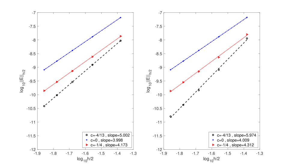
Figure 1: Error and Convergence plots, $\log_{10}\|{{\bf E}}\|$ vs. $\log_{10}h$ for 1D Heat Problem - Dirichlet boundary conditions. Left: without Post-Processing; right: with Post-Processing.

2.4 Conclusion

We combined the advantages of viewing our BFD scheme first as a FE type and secondly as a FD type. This allowed us to provide a proof of stability in an easy manner based on the standard tools developed for DG methods, and then the optimal rate of convergence was proved through the tools developed for BFD methods.

2.5 Generalization to Two Dimensions

The generalization to two dimensions is fairly straightforward, as the two-dimensional scheme is constructed as a tensor product of the one-dimensional scheme presented in the previous subsection.

Let us first consider the following problem with periodic boundary conditions:

$$\left\{\begin{array}[]{ll}\dfrac{\partial u}{\partial t}(x,y,t)=\dfrac{\partial^{2}}{\partial x^{2}}u(x,y,t)+\dfrac{\partial^{2}}{\partial y^{2}}u(x,y,t)+F(x,y,t)\mbox{ , }\\ \hskip 150.00023pt(x,y)\in\left(0,2\pi\right)\times\left(0,2\pi\right)\mbox{ , }t\geq 0\\ u(x,y,t=0)=f(x,y)\end{array}\right.$$ (48)

2.5.1 Proof of Optimal Convergence

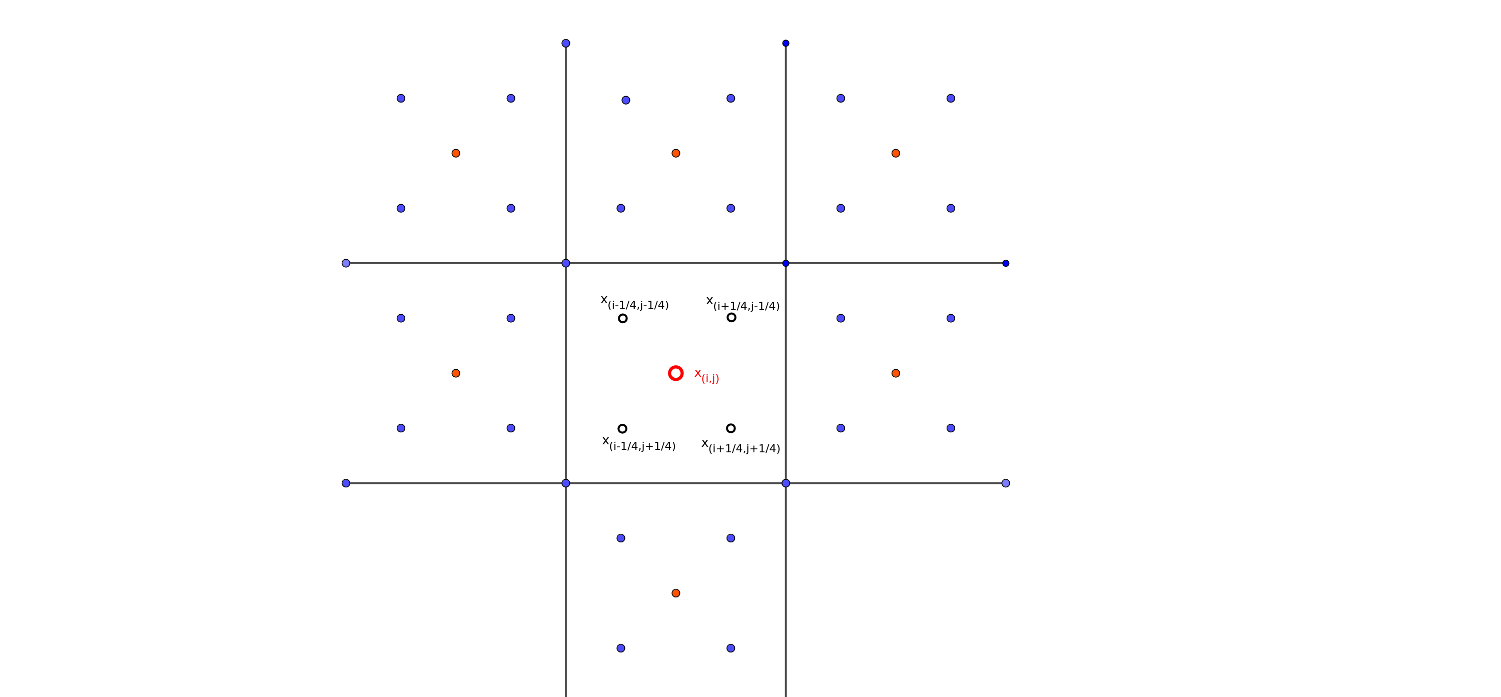
Figure 2: Grid in 2 Dimensions - Illustration

Let us present the two-dimensional 5th order approximation of four-point block. We consider the following grid: In each cell whose center is located in $x_{(i,j)}$, we define four nodes as illustrated in Fig. 2:

$${{\bf x}}_{(i-{1/4},j-{1/4})} = {{\bf x}}_{(i,j)}+\left(-\frac{h}{4},-\frac{h}{4}\right)$$

$${{\bf x}}_{(i+1/4,j+1/4)} = {{\bf x}}_{(i,j)}+\left(\frac{h}{4},\frac{h}{4}\right)$$

$${{\bf x}}_{(i+1/4,j-1/4)} = {{\bf x}}_{(i,j)}+\left(\frac{h}{4},-\frac{h}{4}\right)$$

$${{\bf x}}_{(i-1/4,j+1/4)} = {{\bf x}}_{(i,j)}+\left(-\frac{h}{4},\frac{h}{4}\right)$$ (49)

$$\qquad h=2\pi/N,\;i,j=1,...,N$$

where

$${{\bf x}}_{(i,j)}=\left(h(i-1)+\frac{h}{2},h(j-1)+\frac{h}{2}\right)$$

Altogether there are $4N^{2}$ points on the grid, with a distance of $h/2$ between them when located at the same $x$ or $y$ coordinate.

2.5.2 Proof of Stability

The generalization to higher dimensions is done seamlessly. Indeed, the operator ${\Theta}_{j-1/2}$, as defined in the previous section for one dimension only, can be defined for two or more dimensions. In two dimensions, it is a linear combination of the contributions from each side of the cell and the average of two integrals of one dimension, in the $x$ and $y$ direction, respectively.

Similarly to the one-dimensional case, we may define all $\Theta$ operators in the x and y-directions respectively.

In two dimensions, $\Theta$ is an integral over the edge of the cell. In a rectangular cell, four of those exist (see Fig. 3). Since our approximation space is a tensor product of polynomials degree up to $k$, these integrals can be calculated using a convex combination of values of $u$ at the cell boundaries. In our case, $k=1$, and the linear combination is the average.

Hence, stability in the one-dimensional case implies stability in higher space dimensions.

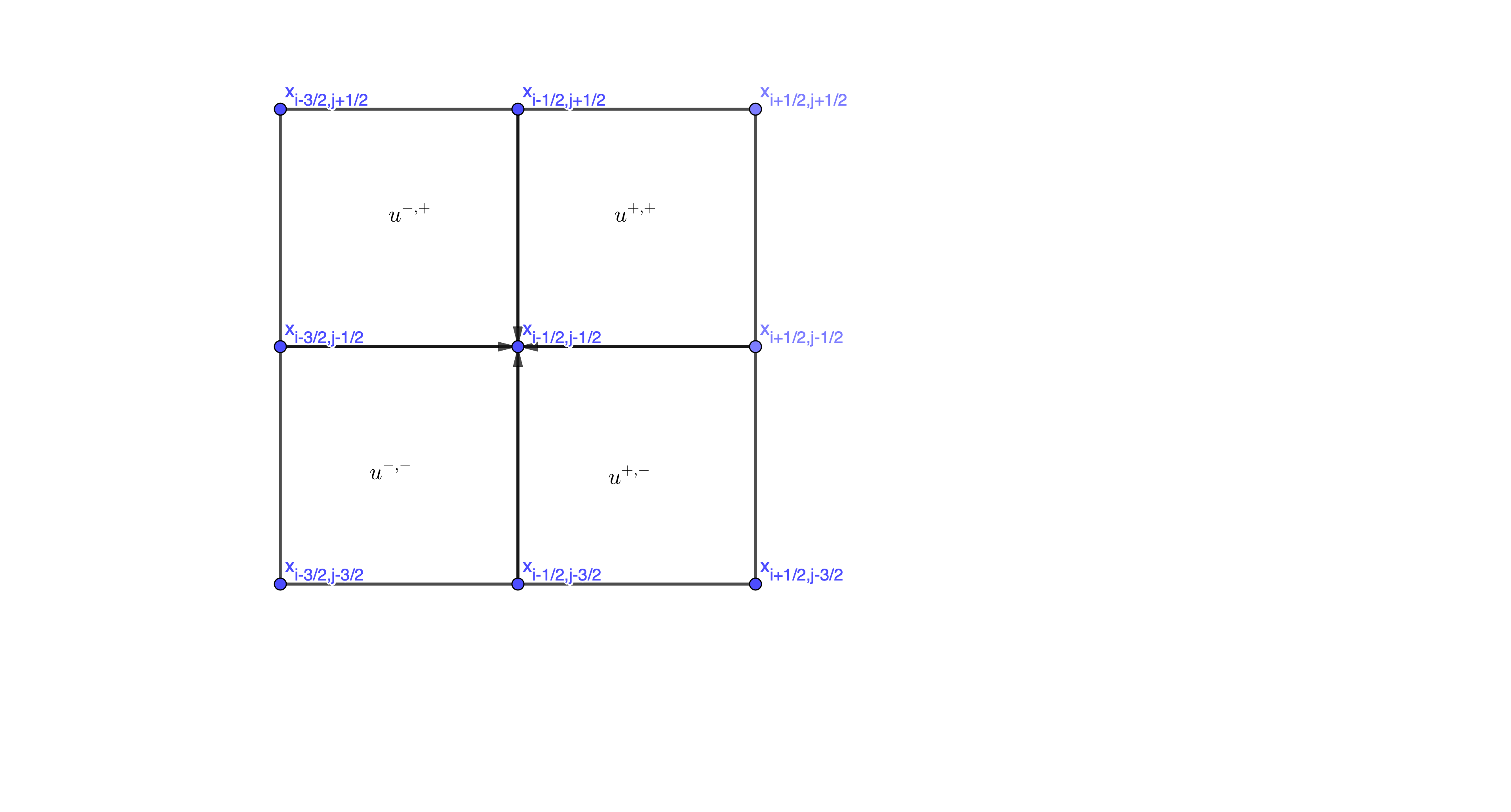
Figure 3: Illustration of the dependence on node ${{\bf x}}_{i-1/2,j-1/2}$ from neighbouring nodes in 2D

2.5.3 Numerical Results

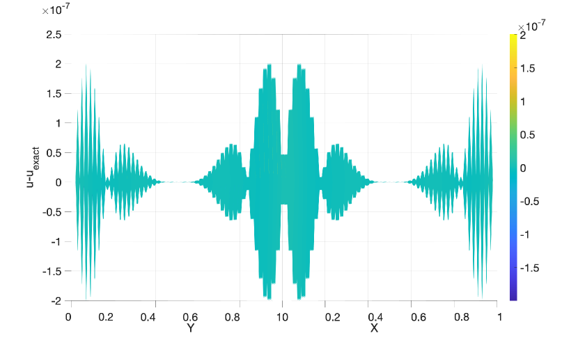
Figure 4: 2D Heat Problem - Two Points Block, BFD scheme - Periodic BC - Error at Final Time $T=1$ - $N=50$ - No post-processing

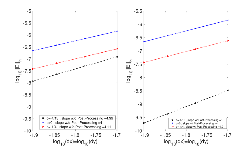
Figure 5: 2D Heat Problem - Two Points Block, BFD scheme, Convergence plots, $\log_{10}\|{{\bf E}}\|$ vs. $\log_{10}h$ - Periodic BC - Left: no post-processing; right: Spectral post-processing

Numerical results demonstrate our theory on stability and order of convergence (see Fig. 4). The scheme was run for $u(x,y,t)=\exp(\cos(2\pi(x+y-t)))$ on the interval $[0,1]\times[0,1]$ and $N=50,60,70,80$ with a 6th order explicit Runge-Kutta time propagator and Final Time $T=1$. In order to clarify the error properties in 2D, the figure pictures the observation at $z=0$ and far from $x=y=0$. In Fig. 5, the convergence plots appear with $c=-4/13,0,-1/4$, and the optimal convergence rate, a fifth order without a with post-processing and a sixth order with one is reached for $c=-4/13$.

2.5.4 Non-Periodic Boundary Conditions

Let us first consider the following two-dimensional Heat Problem with non-periodic boundary conditions:

$$\left\{\begin{array}[]{ll}\dfrac{\partial u}{\partial t}(x,y,t)=\dfrac{\partial^{2}}{\partial x^{2}}u(x,y,t)+\dfrac{\partial^{2}}{\partial y^{2}}u(x,y,t)+F(x,y,t)\mbox{ , }\\ \hskip 150.00023pt(x,y)\in\left(0,\pi\right)\times\left(0,\pi\right)\mbox{ , }t\geq 0\\ u(t=0)=f(x,y)\\ u(0,y,t)=g_{0}(y,t)\\ u(\pi,y,t)=g_{\pi}(y,t)\\ u(x,0,t)=h_{0}(x,t)\\ u(x,\pi,t)=h_{\pi}(x,t)\end{array}\right.$$ (50)

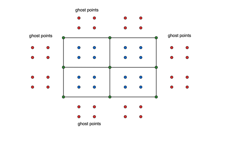
Figure 6: Grid and Ghost Points in 2D - Illustration

In order to get an approximation scheme for the boundary points of the rectangle $[0,\pi]\times[0,\pi]$, we perform an extrapolation for the additional ghost points needed as illustrated in Fig. 6.

In the x-axis direction: ${{\bf x}}_{(\frac{1}{4},j)}=(-\frac{h}{4},y_{j})$, ${{\bf x}}_{(-\frac{1}{4},j)}=(-\frac{3h}{4},y_{j})$ on one end

and ${{\bf x}}_{((N+1)-\frac{1}{4},j)}=(\pi+\frac{h}{4},y_{j})$, ${{\bf x}}_{((N+1)+\frac{1}{4},j)}=(\pi+\frac{3h}{4},y_{j})$ on the other end.

As for the internal points ${{\bf x}}_{i,j}$, $1\leq i,j\leq N$, the scheme remains the same.

It follows that:

$$\left.\begin{array}[]{ll}u_{(-\frac{1}{4},j)}=-u_{(1+\frac{1}{4},j)}+2g_{0}(y_{j},t)+u_{xx}\left(0,y_{j},t\right)\left(\frac{3h}{4}\right)^{2}+\\ \hskip 50.00008pt\frac{1}{12}u_{xxxx}\left(0,y_{j},t\right)\left(\frac{3h}{4}\right)^{4}+O(h^{6})\\ u_{(\frac{1}{4},j)}=-u_{(1-\frac{1}{4},j)}+2g_{0}(y_{j},t)+u_{xx}\left(0,y_{j},t\right)\left(\frac{h}{4}\right)^{2}+\\ \hskip 50.00008pt\frac{1}{12}u_{xxxx}\left(0,y_{j},t\right)\left(\frac{h}{4}\right)^{4}+O(h^{6})\\ \end{array}\right.$$ (51)

Similarly:

$$\left.\begin{array}[]{ll}u_{((N+1)-\frac{1}{4},j)}=-u_{(N+\frac{1}{4},j)}+2g_{\pi}(y_{j},t)+u_{xx}\left(\pi,y_{j},t\right)\left(\frac{h}{4}\right)^{2}+\\ \hskip 50.00008pt\frac{1}{12}u_{xxxx}\left(\pi,y_{j},t\right)\left(\frac{h}{4}\right)^{4}+O(h^{6})\\ u_{((N+1)+\frac{1}{4},j)}=-u_{(N-\frac{1}{4},j)}+2g_{\pi}(y_{j},t)+u_{xx}\left(\pi,y_{j},t\right)\left(\frac{3h}{4}\right)^{2}+\\ \hskip 50.00008pt\frac{1}{12}u_{xxxx}\left(\pi,y_{j},t\right)\left(\frac{3h}{4}\right)^{4}+O(h^{6})\\ \end{array}\right.$$ (52)

where $u_{xx}(0,y_{i},t)$,$u_{xxxx}(0,t)$,$u_{xx}(\pi,y_{i},t)$,$u_{xxxx}(\pi,y_{i},t)$ can be directly computed from the PDE:

$$\left.\begin{array}[]{ll}u_{xx}(0,y,t)=u_{t}(0,y,t)-u_{yy}(0,y,t)-F(0,y,t)\\ u_{xx}(\pi,y,t)=u_{t}(\pi,y,t)-u_{yy}(\pi,y,t)-F(\pi,y,t)\\ u_{xxxx}(0,y,t)=u_{tt}(0,y,t)-2u_{tyy}(0,y,t)-F_{t}(0,y,t)+\\ \hskip 80.00012ptu_{yyyy}(0,y,t)+F_{yy}(0,y,t)-F_{xx}(0,y,t)\\ u_{xxxx}(\pi,y,t)=u_{tt}(\pi,y,t)-2u_{tyy}(\pi,y,t)-F_{t}(\pi,y,t)+\\ \hskip 80.00012ptu_{yyyy}(\pi,y,t)+F_{yy}(\pi,y,t)-F_{xx}(0,y,t)\\ \end{array}\right.$$ (53)

In the $y$-axis direction, the extrapolations are analogous.

2.5.5 Numerical Results

Figure 7: 2D Heat Problem - Two Points Block, BFD scheme - Dirichlet BC - Error at Final Time $T=1$ - $N=72$ - No post-processing

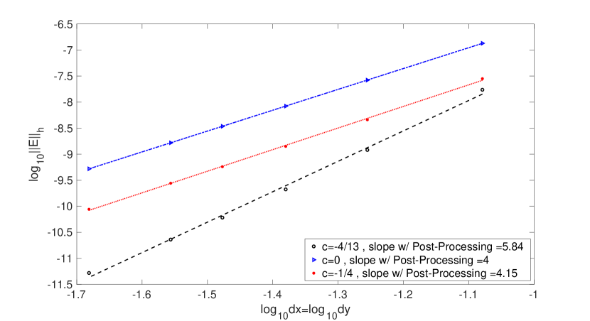
Figure 8: 2D Heat Problem - Two Points Block, BFD scheme, Convergence plots, $\log_{10}\|{{\bf E}}\|$ vs. $\log_{10}h$ - Dirichlet BC -post-processing filter

Numerical results demonstrate our theory on stability and order of convergence (see Fig. 7). The scheme was run for an exact solution $u(x,y,t)=\exp(\cos(x+y-t))$ on the interval $[0,1]\times[0,1]$ and $N=24,36,48,60,72,96$ with a sixth order explicit Runge-Kutta time propagator and Final Time $T=1$. In order to clarify the error properties in 2D, the figure pictures the view from an observer at $z=0$ and far from $x=y=0$.

The convergence plots present for $c=0,-1/4,-4/13$ BFD schemes, are presented in Fig. 8. The same optimal convergence rate is reached for $c=-4/13$, resulting in a sixth-order convergence rate with a post-processing filter. The scheme was run for an exact solution $u(x,y,t)=\exp(\cos(x+y-t))$ on the interval $[0,1]\times[0,1]$ and $N=24,36,48,60,72,96$ with a sixth-order explicit Runge-Kutta time propagator and Final Time $T=1$.

2.6 Generalization to Three Dimensions

In this section, we present a brief description of the three-dimensional BFS/GD scheme.

Consider the Heat equation with periodic boundary conditions:

$$\left\{\begin{array}[]{ll}\dfrac{\partial u}{\partial t}(x,y,zt)=\nabla^{2}u(x,y,z,t))+F(x,y,t)\mbox{ , }\\ \hskip 100.00015pt{{\bf x}}=(x,y,z)\in\left(0,2\pi\right)\times\left(0,2\pi\right)\times\left(0,2\pi\right)\mbox{ , }t\geq 0\\ u(x,y,z,t=0)=f(x,y,z)\end{array}\right.$$ (54)

The domain is divided into cells, $I_{(j,k,l)}$, where

$$I_{(j,k,l)}=\left\{{{\bf x}}:\left|x-x_{(j,k,l)}\right|,\left|y-y_{(j,k,l)}\right|,\left|z-z_{(j,k,l)}\right|\leq\frac{h}{2}\right\}$$ (55)

and

$${{\bf x}}_{(j,k,l)}=\left(x_{(j,k,l)},y_{(j,k,l)},z_{(j,k,l)}\right)=\left(h(j-1)+\frac{h}{2},h(k-1)+\frac{h}{2},h(l-1)+\frac{h}{2}\right)$$ (56)

The grid points, at each cell, are

$${{\bf x}}_{(j\pm 1/4,k\pm 1/4,l\pm 1/4)}={{\bf x}}_{(j,k,l)}+\left(\pm 1,\pm 1,\pm 1\right)\frac{h}{4}$$ (57)

Altogether, there are eight grid points at each cell.

These nodes form a rectangular grid aligned with the axes. The one-dimensional BFD scheme, (16), is used for each line parallel to the $x$, $y$, and $z$. This three-dimensional scheme is stable since the operator $\Theta$ at each face of the cells $I_{(j,k,l)}$ is a convex combination of the non-positive one-dimensional $\Theta$. Thus, it is non-positive as well.

For the non-periodic boundary conditions, as for the two-dimensional case, to approximate the values at the boundary points of the cube $[0,\pi]\times[0,\pi]\times[0,\pi]$, we perform an extrapolation to obtain the additional ghost points. The formulation for these extrapolations and the proofs are similar to the one- and two-dimensional cases.

3 Future Work

The schemes we constructed and analyzed in this manuscript are defined in rectangular domains. Our project’s next stage is to derive block finite difference schemes to solve the heat equation in two and three-dimensional, complicated geometries.

We also intend to derive block finite difference schemes to solve the advection equation and hyperbolic systems.

4 Acknowledgement

This research was supported by Binational (US-Israel) Science Foundation grant No. 2016197.

Appendix A Pseudo-Fourier Analysis - Eigenvalues and Eigenvectors

This section will use tools developed in [5] and [6]. The goal of the procedure is to find a value of the parameter $c$ that appears in the BFD scheme (2.1), leading to the optimal convergence rate of this scheme.
We will perform a Fourier-like analysis for this purpose. In [7], a straightforward Fourier analysis was performed using different equations with periodic boundary conditions. Here, the analysis of the error structure basis is a linear combination of eigenvectors, hence covering the case where the matrix $Q$ is not diagonalizable using standard discrete Fourier transform. The analysis still requires periodic boundary conditions and a uniform mesh.

We first split the Fourier spectrum into low and high frequencies as follows: Let $\omega\in\{-N/2,\ldots,N/2$} being an integer and :

$$\nu\,=\,\left\{\begin{array}[]{lcl}\omega-N,&\omega>0\\ \omega+N,&\omega\leq 0\end{array}\right.$$ (58)

Then,

$$\text{for }\omega\geq 0: e^{i\nu x_{j-1/4}}=-ie^{i\omega x_{j-1/4}}\;\;{\rm and}\;\;e^{i\nu x_{j+1/4}}=ie^{i\omega x_{j+1/4}}$$ (59)

$$\text{for }\omega<0: e^{i\nu x_{j-1/4}}=ie^{i\omega x_{j-1/4}}\;\;{\rm and}\;\;e^{i\nu x_{j+1/4}}=-ie^{i\omega x_{j+1/4}}$$

We now present thae analysis for $\omega\geq 0$. The analysis for $\omega<0$ is similar.

We denote the vectors ${\rm e}^{i\omega\bm{x}}$ and ${\rm e}^{i\nu\bm{x}}$ by:

$${\rm e}^{i\omega\bm{x}}=\left(\begin{array}[]{c}\vdots\\ {\rm e}^{i\omega x_{j-{1/4}}}\\ {\rm e}^{i\omega x_{j+1/4}}\\ \vdots\end{array}\right)\mbox{, }{\rm e}^{i\nu\bm{x}}=\left(\begin{array}[]{c}\vdots\\ {\rm e}^{i\nu x_{j-{1/4}}}\\ {\rm e}^{i\nu x_{j+1/4}}\\ \vdots\end{array}\right)$$ (60)

We look for eigenvectors in the form of:

$$\psi_{k}(\omega)={\alpha_{k}}\frac{{\rm e}^{i\omega\bm{x}}}{\sqrt{2\pi}}+{\beta_{k}}\frac{{\rm e}^{i\nu\bm{x}}}{\sqrt{2\pi}}$$ (61)

where, for normalization, it is required that $|\alpha_{k}|^{2}+|\beta_{k}|^{2}=1$, $k=1,2$.

We note here that each component of the linear combination ${\rm e}^{i\omega\bm{x}}$ and ${\rm e}^{i\nu\bm{x}}$ is not an eigenvector in the classical sense, since only the linear combination verifies the initial condition.

However:

$$Q{\rm e}^{i\omega\bm{x}}={\rm diag}({\mu}_{1},{\mu}_{2},...,{\mu}_{1},{\mu}_{2}){\rm e}^{i\omega\bm{x}}$$ (62)

$$Q{\rm e}^{i\nu\bm{x}}={\rm diag}({\sigma}_{1},{\sigma}_{2},...,{\sigma}_{1},{\sigma}_{2}){\rm e}^{i\nu\bm{x}}$$ (63)

where:

$$\mu_{1} = \frac{8}{3h^{2}}\left[-{\sin^{2}\left(\frac{h\omega}{4}\right)\left(7-\cos\left(\frac{h\omega}{2}\right)\right)}-4\,i\,c\,e^{\frac{ihw}{4}}\sin^{5}\left(\frac{hw}{4}\right)\right]$$

$$\mu_{2} = \frac{8}{3h^{2}}\left[-{\sin^{2}\left(\frac{h\omega}{4}\right)\left(7-\cos\left(\frac{h\omega}{2}\right)\right)}+4\,i\,c\,e^{-\frac{ihw}{4}}\sin^{5}\left(\frac{hw}{4}\right)\right]$$

$$\sigma_{1} = \frac{8}{3h^{2}}\left[{-\cos^{2}\left(\frac{h\omega}{4}\right)\left(7+\cos\left(\frac{h\omega}{2}\right)\right)}+4\ c\,e^{\frac{ihw}{4}}\cos^{5}\left(\frac{hw}{4}\right)\right]$$

$$\sigma_{2} = \frac{8}{3h^{2}}\left[{-\cos^{2}\left(\frac{h\omega}{4}\right)\left(7+\cos\left(\frac{h\omega}{2}\right)\right)}+4\ c\,e^{-\frac{ihw}{4}}\cos^{5}\left(\frac{hw}{4}\right)\right]$$

In order to find the coefficients ${\alpha}_{k}$ and ${\beta}_{k}$ along with the eigenvalues (symbols) $\hat{Q}_{k}$ for $\omega>0$, we consider some node $x_{j}$. Then we solve the following system of equations:

$$\left.\begin{array}[]{ll}{\mu}_{1}\frac{\alpha_{k}}{\sqrt{2\pi}}{\rm e}^{i\omega{x_{j-\frac{1}{4}}}}+{\sigma}_{1}\frac{\beta_{k}}{\sqrt{2\pi}}{\rm e}^{i\nu{x_{j-\frac{1}{4}}}}={\hat{Q}}_{k}\left(\frac{\alpha_{k}}{\sqrt{2\pi}}{\rm e}^{i\omega{x_{j-\frac{1}{4}}}}+\frac{\beta_{k}}{\sqrt{2\pi}}{\rm e}^{i\nu{x_{j-\frac{1}{4}}}}\right)\\ {\mu}_{2}\frac{\alpha_{k}}{\sqrt{2\pi}}{\rm e}^{i\omega{x_{j+\frac{1}{4}}}}+{\sigma}_{2}\frac{\beta_{k}}{\sqrt{2\pi}}{\rm e}^{i\nu{x_{j+\frac{1}{4}}}}={\hat{Q}}_{k}\left(\frac{\alpha_{k}}{\sqrt{2\pi}}{\rm e}^{i\omega{x_{j+\frac{1}{4}}}}+\frac{\beta_{k}}{\sqrt{2\pi}}{\rm e}^{i\nu{x_{j+\frac{1}{4}}}}\right)\end{array}\right.$$ (65)

We denote $r_{k}=i\dfrac{{\beta}_{k}}{{\alpha}_{k}}$ and use Eq. (59) to obtain a simpler system:

$$\left.\begin{array}[]{ll}{\mu}_{1}-{\sigma}_{1}r_{k}={\hat{Q}}_{k}\left(1-r_{k}\right)\\ {\mu}_{2}+{\sigma}_{2}r_{k}={\hat{Q}}_{k}\left(1+r_{k}\right)\\ \end{array}\right.$$ (66)

Consequently, the expressions for $r_{k}$ and the eigenvalues (symbols) $\hat{Q}_{k}$ are:

$$\left.\begin{array}[]{ll}r_{1}=\dfrac{\Omega+\Delta}{16c\sin\left(\frac{h\omega}{4}\right)\cos^{5}\left(\frac{h\omega}{4}\right)}i\\ \\ r_{2}=\dfrac{\Omega-\Delta}{16c\sin\left(\frac{h\omega}{4}\right)\cos^{5}\left(\frac{h\omega}{4}\right)}i\\ \\ \end{array}\right.$$ (67)

where

$$\Omega = -\cos\left(\frac{h\omega}{2}\right)\Big{(}16-\Big{(}7+\cos\left(h\omega\right)\Big{)}c\Big{)}$$ (68)

and

$$\Delta = \sqrt{\Omega^{2}+4c^{2}\sin^{6}\left(\frac{h\omega}{2}\right)}$$ (69)

The symbols $\hat{Q}_{1}(\omega)$ and $\hat{Q}_{2}(\omega)$ are:

$$\left.\begin{array}[]{ll}\hat{Q}_{1}(\omega)=\dfrac{2}{3h^{2}}\Big{(}-\Big{(}15+\cos(h\omega)\Big{)}+\Big{(}5+3\cos(h\omega)\Big{)}c+\Delta\Big{)}\mbox{, }\\ \\ \hat{Q}_{2}(\omega)=\dfrac{2}{3h^{2}}\Big{(}-\Big{(}15+\cos(h\omega)\Big{)}+\Big{(}5+3\cos(h\omega)\Big{)}c+\Delta\Big{)}\\ \end{array}\right.$$ (70)

Using the normalization condition $|\alpha_{k}|^{2}+|\beta_{k}|^{2}=1$, $k=1,2$, we choose the coefficients ${\alpha}_{k},{\beta}_{k}$ to be:

$$\alpha_{1}=\dfrac{1}{\sqrt{1+{|r_{1}|}^{2}}}\mbox{, }\beta_{1}=-i\dfrac{r_{1}}{\sqrt{1+{|r_{1}|}^{2}}}\\$$ (71)

$$\alpha_{2}=i\dfrac{r_{2}/|r_{2}|}{\sqrt{1+{|r_{2}|}^{2}}}\mbox{, }\beta_{2}=\dfrac{|r_{2}|}{\sqrt{1+{|r_{2}|}^{2}}}$$ (72)

It is important to note here that all eigenvalues $\hat{Q}_{1}$ and $\hat{Q}_{2}$ are real and non-positive for all $\omega$ and $|c|\leq 1$. Therefore, the scheme is Von-Neumann stable. Additionally, since a complete set of eigenvectors exists, we conclude that the scheme is stable.

For $\omega h\ll 1$ the eigenvalues are:

$$\hat{Q}_{1}(\omega)=-\omega^{2}+\dfrac{(4+13c)\omega^{6}{h}^{4}}{2880(2-c)}-\dfrac{(4+38c+c^{2})\omega^{8}h^{6}}{64512(2-c)^{2}}+O(h^{8})\\$$ (73)

and

$$\hat{Q}_{2}(\omega)=-\dfrac{32(2-c)}{3h^{2}}+\dfrac{(5-6c)\omega^{2}}{3}-\dfrac{(1-3c)\omega^{4}h^{2}}{18}+O(h^{4})$$ (74)

Since $\hat{Q}_{2}(\omega)=O(1/h^{2})$ is negative, it immediately decays. Therefore ,we can neglect the $\psi_{2}$ terms.

If the initial condition is $u(x,t=0)={\rm e}^{i\omega x}/\sqrt{2\pi}$, i.e.

$${{\bf v}}_{j-\frac{1}{4}}(0)={\rm e}^{i\omega x_{j-\frac{1}{4}}}/\sqrt{2\pi}\;,{{\bf v}}_{j+\frac{1}{4}}(0)={\rm e}^{i\omega x_{j+\frac{1}{4}}}/\sqrt{2\pi}\;\;;\;\;\;\;\omega^{2}h\ll 1$$ (75)

Then

$$\left.\begin{array}[]{ll}{{{\bf v}}}_{j-\frac{1}{4}}(t)=\left({\rm e}^{-\omega^{2}t}\left[1+\dfrac{(4+13c){\omega}^{6}{h}^{4}}{2880(2-c)}t\right]+O(h^{6})\right)\dfrac{{\rm e}^{i\omega x_{j-\frac{1}{4}}}}{\sqrt{2\pi}}+\\ \\ \hskip 80.00012pt\left(\dfrac{c\,{\rm e}^{-\omega^{2}t}({\omega h})^{5}}{1024(2-c)}+O(h^{6})\right)\dfrac{{\rm e}^{i\nu x_{j-\frac{1}{4}}}}{\sqrt{2\pi}}\end{array}\right.$$ (76)

The same expression holds for $x_{j+1/4}$. The scheme is of fourth-order in general. However, if $c=-4/13$, then it becomes fifth-order. Furthermore, upon closer inspection of equation (76), it appears that the error term’s leading coefficient is of high frequency for the $c=-4/13$ case. This suggests that applying a post-processing filter can remove this high-frequency error, resulting in a sixth-order convergence rate.

Appendix B Post-processing

The analysis presented in A demonstrates that when the initial condition is $u(x,t=0)=\exp(i\omega x)$ and $\omega h\ll 1$, the numerical solution at time $t_{n}$ can be calculated using equation (76). This scheme is of fourth-order, but selecting $c=-4/13$ eliminates the leading term in error, resulting in a fifth-order convergence rate. We now observe that the fifth-order term is of high frequency; therefore, it can be filtered in a post-processing stage to get a sixth-order scheme. This section describes the construction of these post-processing filters.

B.1 Post-Processing applied to Heat problem with Periodic Boundary Conditions

The analysis in A showed that the sixth-order convergence rate could be recovered by choosing $c=-4/13$ and filtering the high-frequency Fourier modes (larger than $N/2$ in absolute value) at a post-processing stage.

Thus, for the one-dimensional problem, the post-processing filtering is done as follows:

1. Computing the discrete Fourier transform (DFT) of the numerical solution at the final time, ${{\bf v}}^{n}$.

2. Zeroing the coefficients of the high-frequency modes.

3. Computing the inverse discrete Fourier transform.

In the two-dimensional case, this procedure is performed for every row and column.

B.2 Post-Processing for Non-periodic boundary conditions of Dirichlet type

We look for a one-step procedure leading to an increased order of accuracy. Unlike the case of periodic boundary conditions, the filter presented above cannot be used. Hence, a different technique shall be applied. Those filters were derived from a class of filters specifically applied to DG methods in the case of hyperbolic problems (see [13], [9], [2]), and compared with the standard Savitzky-Golay Filter [14].

B.2.1 Filter Description

This section is dedicated to the description of the three filters that were used, starting with the standard filter Savitzky-Golay Filter [14].

Savitzky-Golay Filter

Since their introduction more than half a century ago, Savitzky–Golay (SG) filters have been popular in many fields of data processing. They use a method of data smoothing based on local least-squares polynomial approximation. SG filters are usually applied to equidistant data points and are based on fitting a polynomial of a given degree $n$ to the data in a (usually symmetric) neighborhood $k-m...k+m$ of each data point $k$. This range contains $2m+1$ data points. Each data point is replaced by the value of the fit polynomial at this point $k$. As this process is a linear filter and takes a limited number of points as the input, SG smoothing belongs to the class of Finite Impulse Response (FIR) filters. Therefore, it can be implemented as a convolution with a suitable kernel.

The filter was used as a benchmark for our custom filter, with the parameters $n=6,m=5$, using Matlab©[12] sgolayfilt tool.
We note here that $m$ is limited to odd values in order to conserve the symmetry of the interpolation. Asymmetric filters can be designed, but their efficiency does not increase [11].

Numerical results will show that this filter is efficient from the error reduction aspect, but does not affect the order of accuracy of the BFD scheme.

In the next paragraph, we try and design filters based on a different kernel.

First Interpolation Filter

For every set of the 12 consecutive grid points, we perform an interpolation procedure of the approximated solution valued at those grid nodes to obtain a sixth-order interpolation polynomial (for the optimal $c=-4/13$ case).

We then compute the related approximation for the set of points and proceed to the next set of 12 nodes. This is in contrast with the SG filter, where each node is approximated by a different polynomial.

Since the post-processed error is still somewhat oscillatory, a second version of an interpolation filter is designed in the following paragraph.

Second Interpolation Filter

This time, the first six points from the left are interpolated as before. Then, the filtered values of each set of two points are taken as the six-order interpolation based on these two points, five points from the left and five from the right. The last six points are computed similarly to the first six. There is a significant improvement in the Final Time error, as illustrated in Fig. 9. A seventh order of convergence is reached.

B.2.2 Post-Processing Numerical Results

We employed the approximation (2.3.1)-(2.3.1) to find the solution to the heat problem (35) on the interval $[0,1]$. We chose $F(x,t)$ and the initial condition in such a way that the exact solution is $u(x,t)=\exp(\cos(x-t))$. The scheme was executed for various values of $N$, specifically $N=24,36,48,72,84$. We used a sixth-order explicit Runge-Kutta method for time integration, with a small time step, and a Final Time of $T=1$.

(a) Error plots at Final Time $T=1$ with $N=18$ (36 grid points)

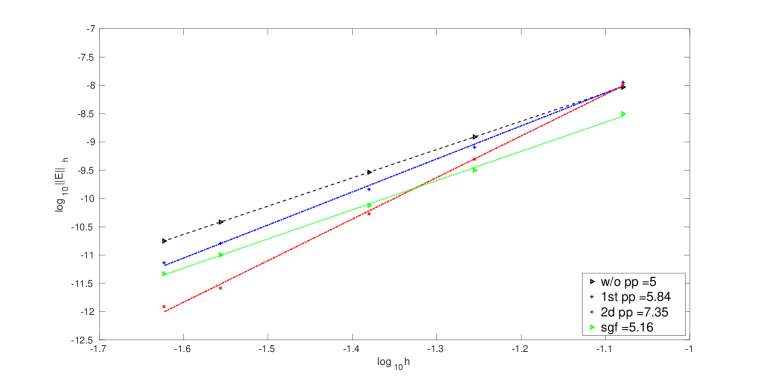
(b) Convergence plots with no post-processing, First and Second Interpolation filters, SG Filter.

Figure 9: 1D Heat Problem - Two Points Block, BFD scheme - Dirichlet BC - $c=-4/13$.

The standard SG filter effectively reduces the error but does not affect the order of convergence. Our customized filters are less efficient as far as the error reduction for small $N$, but increase the rate of convergence to seven instead of five, as illustrated in Fig. 9.
We note here that further improvements on the issue of filters are left for future research.

References

• [1] Generalized Window Method. https://ccrma.stanford.edu/~jos/sasp/Generalized_Window_Method.html.
• [2] C.-W. Shu B. Cockburn, M. Luskin and E. Süli. Enhanced accuracy by post-processing for finite element methods for hyperbolic equations. Mathematics of Computation, (72):577–606, 2003.
• [3] I. Babuska, C.E. Baumann, and J.T. Oden. A discontinuous hp finite element method for diffusion problems: 1-d analysis. Computers & Mathematics with Applications, 37(9):103 – 122, 1999.
• [4] SC. E. Baumann and J. T. Oden. A discontinuous hp finite element method for convection-diffusion problems. Comput. Methods Appl. Mech. Engrg., (175):311–341, 1999.
• [5] Adi Ditkowski. High order finite difference schemes for the heat equation whose convergence rates are higher than their truncation errors. In Spectral and High Order Methods for Partial Differential Equations ICOSAHOM 2014, pages 167–178. Springer, 2015.
• [6] Adi Ditkowski and Paz Fink Shustin. Error inhibiting schemes for initial boundary value heat equation. 2020. https://arxiv.org/abs/2010.00476.
• [7] Wei Guo, Xinghui Zhong, and Jing-Mei Qiu. Superconvergence of discontinuous galerkin and local discontinuous galerkin methods: Eigen-structure analysis based on fourier approach. Journal of Computational Physics, 235:458–485, 2013.
• [8] Bertil Gustafsson, Heinz-Otto Kreiss, and Joseph Oliger. Time dependent problems and difference methods, volume 24. John Wiley & Sons, 1995.
• [9] C.-W. Shu J. Ryan and H. Atkins. Extension of a post processing technique for the discontinuous galerkin method for hyperbolic equations with application to an aeroacoustic problem. J. Sci. Comput., (26(3)):821–843, 2005.
• [10] Peter D Lax and Robert D Richtmyer. Survey of the stability of linear finite difference equations. Communications on pure and applied mathematics, 9(2):267–293, 1956.
• [11] J. Luo, K. Ying, and L. Bai. Savitzky–golay smoothing and differentiation filter for even number data. Signal Processing, 85:1429–1434, 2005.
• [12] MATLAB. version 9.11.0 (R2021b). The MathWorks Inc., Natick, Massachusetts, 2021.
• [13] J. K. Ryan. Exploiting superconvergence through smoothness-increasing accuracy-conserving (siac) filtering. In Spectral and High Order Methods for Partial Differential Equations ICOSAHOM 2014, pages 87–102. Springer International Publishing, 2015.
• [14] A. Savitzky and M. J. E. Golay. Smoothing and differentiation of data by simplified least squares procedures. Analytical Chemistry, 36(8):1627–1639, 1964.
• [15] Chi-Wang Shu. Discontinuous galerkin methods: general approach and stability. Numerical solutions of partial differential equations, 201, 2009.
• [16] James J. Sylvester. A demonstration of the theorem that every homogeneous quadratic polynomial is reducible by real orthogonal substitutions to the form of a sum of positive and negative squares. Philosophical Magazine Series, 4(23):138–142, 1852.
• [17] Mengping Zhang and Chi-Wang Shu. An analysis of three different formulations of the discontinuous galerkin method for diffusion equations. Mathematical Models and Methods in Applied Sciences, 13(03):395–413, 2003.