Dual-Domain Deep D-bar Method for Solving Electrical Impedance Tomography

Abstract

The regularized D-bar method is one of the most prominent methods for solving Electrical Impedance Tomography (EIT) problems due to its efficiency and simplicity. It provides a direct approach by applying low-pass filtering to the scattering data in the non-linear Fourier domain, thereby yielding a smoothed conductivity approximation. However, D-bar images often present low contrast and low resolution due to the absence of accurate high-frequency information and ill-posedness of the problem. In this paper, we proposed a dual-domain neural network architecture to retrieve high-contrast D-bar image sequences from low-contrast D-bar images. To further accentuate the spatial features of the conductivity distribution, the widely adopted U-net has been tailored for conductivity image calibration from the predicted D-bar image sequences. We call such a hybrid approach by Dual-Domain Deep D-bar method due to the consideration of both scattering data and image information. Compared to the single-scale structure, our proposed multi-scale structure exhibits superior capabilities in reducing artifacts and refining conductivity approximation. Additionally, solving discrete D-bar systems using the GMRES algorithm entails significant computational complexity, which is extremely time-consuming on CPU-based devices. To remedy this, we designed a surrogate GPU-based Richardson iterative method to accelerate the data enhancement process by D-bar. Numerical results are presented for simulated EIT data from the KIT4 and ACT4 systems to demonstrate notable improvements in absolute EIT imaging quality when compared to existing methodologies.

Keywords Electrical impedance tomography  $\cdot$ D-bar regularization  $\cdot$ Multi-scale method  $\cdot$ Scattering transformation

1 Introduction

1.1 Problem Setting

Electrical Impedance Tomography (EIT) stands as a remarkable imaging technique that has garnered significant attention within the intersection of mathematics, artificial intelligence, and medical technology. This non-invasive method harnesses the principles of electrical conductivity to unveil the inner workings of objects and organisms, which has been used in fields like non-destructive medical monitoring [1], industrial detection [2] and geophysics [3]. Specifically, EIT involves the application of distinct voltage patterns through electrodes placed on the object’s surface, and the subsequent measurement of resulting current distributions. The ultimate objective is to unveil the internal conductivity distribution of the subject under examination [4].

The mathematical model for the Electric Impedance Tomography (EIT) problem is formulated as the well-known Calderón inverse problem. In our context, we direct our attention to a positive conductivity function $\sigma(z)\in L^{\infty}$ defined on a bounded domain $\Omega$ in $\mathrm{R}^{n}$ with a continuous boundary $\partial{\Omega}$ in $\mathrm{R}^{n-1}$, where $\sigma(z)$ is assumed to be one near the $\partial{\Omega}$ so that it can be naturally extended to the entire space $\mathrm{R}^{n}$. In the specific case of a continuous Dirichlet boundary condition, we suppose that $2N+1$ linearly independent voltage patterns $\{f_{k}\}^{N}_{k=-N}$ are applied to $\partial{\Omega}$, the ensuing electric potential field $u_{k}(z)$ satisfies the following second-order elliptical PDEs

$$\begin{array}[]{cc}\nabla\cdot[\sigma(z)\nabla u_{k}(z)]=0,&\quad z\in\Omega,\\ u_{k}(z)=f_{k}(z),&\quad z\in\partial\Omega.\end{array}$$ (1)

where this set of $2N+1$ equations share a common isotropic conductivity denoted as $\sigma(z)$, a strictly positive function. These equations yield a collection of Cauchy data pairs $\{f_{k},\sigma\frac{\partial u_{k}}{\partial n}|_{\partial\Omega}\}^{N}_{k=-N}$ which plays a crucial role in enabling the retrieval of $\sigma(z)$ within the domain $\Omega$. Generally speaking, the Dirichlet to Neumann (DtN) map, intricately linked to the EIT equation, is defined by

$$\Lambda_{\sigma}:\left.\left.u\right|_{\partial\Omega}\in H^{1/2}(\partial\Omega)\longrightarrow\sigma\frac{\partial u}{\partial n}\right|_{\partial\Omega}\in\widetilde{H}^{-1/2}(\partial\Omega).$$ (2)

Theoretically, according to Nachman’s 1996 global uniqueness proof [5], once the complete knowledge of the DtN map $\Lambda_{\sigma}$ is available, the conductivity distribution $\sigma(z)\in L^{\infty}(\Omega)$ can be uniquely determined. However, in practice, the EIT reconstruction problem is a non-linear inverse problem with severe ill-posedness. This implies that the underlying parameter distribution is highly sensitive to measurement noise and modeling errors [4]. As a result, there exists a significant gap between the ideal theoretical scenario and real-world applications, where only a finite-dimensional matrix approximation of the DtN map, contaminated with noise, can be obtained. Given the inherent ill-posedness of the problem, it becomes crucial to incorporate prior knowledge about the underlying parameter distribution to regularize the conductivity structure and achieve improved reconstruction results.

1.2 Related work

Various traditional numerical algorithms have been developed to tackle the inherent ill-posed nature of the problem. These methods can be broadly classified into two categories: iterative optimization techniques and direct reconstruction approaches. Optimization-based methods typically involve minimizing a data discrepancy term, which quantifies the mismatch between predicted data and actual boundary measurements. These approaches necessitate the use of numerically stable solvers for the forward model with high precision, as well as various regularization techniques [6, 7, 8]. From an optimization standpoint, achieving a satisfactory reconstruction relies not only on a proper initial condition but also on robust optimization strategies, such as regularized Newton-type optimization methods [9, 10], level-set based shape optimization methods [11, 12], subspace-based optimization methods [13, 14], and particle swarm optimization methods [15]. It is worth noting that one of the primary limitations of iterative methods lies in their computational demands and susceptibility to measurement noise and modeling errors [16]. In contrast, non-iterative methods directly reconstruct the conductivity from measurement data, offering advantages in terms of speed and efficiency when compared to the iterative methods. Examples of these direct methods encompass the factorization method [17, 18], the direct sampling method [19], the enclosure method [20], and the D-bar method [4, 21, 22], which often boast elegant mathematical foundations.

In addition to the classical algorithms in EIT, there has been a surge of interest in leveraging supervised learning techniques to address the challenges associated with EIT reconstruction. One main class among these aims to harness the property of the non-linear inverse problem itself and further integrate the learning techniques into the well-established direct methods. Building upon linear perturbative analysis of the EIT forward problem, Fan et al. [23] introduced a compact neural network architecture based on BCR-net [24] to explore the numerically low-rank property of the forward and inverse maps. Guo et al. [25] combined the direct sampling method (DSM) [19] and deep learning techniques to achieve high-quality reconstruction with the ability to incorporate multiple Cauchy data pairs. Hamilton et al. [26, 27] explored the use of deep learning as a post-processing step for regularized D-bar reconstructions, offering the promise of improved real-time reconstruction. Another important class refers to the deep unrolling techniques for solving linear inverse problems, which could be further tailored for non-linear cases. In [28], deep unrolling networks was utilized in computational EIT, where the learned half-quadratic splitting (HQSNet) algorithm was proposed for incorporating physics into learning-based EIT imaging. Besides, Wei et al. [16] also introduced a novel approach by integrating the bases-expansion subspace optimization method (SOM) into a deep learning scheme, effectively creating an iterative-based inversion method that yielded promising results for challenging inclusions. These hybrid deep learning frameworks, which amalgamate the strengths of model-driven and data-driven approaches, have gathered significant attention in the field. However, it’s important to note that the performance of these supervised learning methods heavily relies on their generalization abilities, which may pose challenges when extensive training data is not readily available in practical applications. To circumvent these limitations, researchers have also investigated unsupervised learning approaches based on the physics-informed neural network (PINN) paradigm [29, 30] and the deep image prior (DIP) [22]. These efforts highlight the pursuit of more robust EIT reconstruction techniques that draw from both physics principles and machine learning capabilities.

Figure 1: From an insightful viewpoint, the D-bar regularization method belongs to direct reconstruction approaches for EIT.

1.3 Main Contributions

Among various algorithms, the regularized D-bar method based on the non-linear Fourier transform has emerged as a successful approach for direct EIT reconstruction, owing to its computational effectiveness and high robustness to noise (as illustrated in Fig.1). Motivated by its capability to partition the non-linear frequency domain into stable and unstable parts [4], we introduce a dual-domain learning approach designed for EIT image reconstruction. The main idea is to enhance the scattering data in the frequency domain at varying resolutions and calibrate D-bar images in the image domain with two multi-scale neural networks. In particular, the original low-contrast D-bar image is first enhanced by the images generated from the corresponding ground truth at varying radii $R$ in the scatter transform domain. Secondly, the D-bar image sequence enhanced at the frequency domain is further calibrated through a modified U-net architecture to produce the ultimate high-quality EIT reconstruction. It features the following primary aspects:

• Computational efficiency. Different from the conventional optimization-based methods and unrolling learning approaches for inverse problem reconstruction, this method avoids multiple forward and backward equations solving, which allows for fast training and reconstruction.

• Multi-scale structure. The high-contrast D-bar images are enhanced in the frequency domain for different increased truncation radii. At each resolution level, the combined U-net architecture is tailored to utilize each of them for guided learning in the image domain.

• D-bar method acceleration. Due to the numerical hurdles for solving the scattering transformation and the D-bar integral equations, two remedies for executing on GPU hardware are introduced to further improve the D-bar reconstruction speed.

Numerical experiments show notable reconstruction quality improvements across the KIT4 and ACT4 datasets, compared to the other methods, including both conventional approaches and learning-based D-bar method [26]. These results indicate that the proposed strategy could effectively combine the advantages of both the DL-based methods and the direct methods to achieve high-quality and fast EIT reconstruction.

The remainder of the paper is organized as follows. In Section 2, we will provide a concise overview of the regularized D-bar method. Building upon the principles of the D-bar method, Section 3 will introduce our proposed dual-domain deep D-bar method to resolve the high-contrast D-bar image sequence, followed by an image domain calibration module for ultimate EIT prediction. Subsequently, Section 4 to Section 6 will present comprehensive details of our experiments, numerical results, and ablation studies. Finally, in Section 7, we will summarize our findings and draw conclusions based on the study.

2 Regularized D-bar Method

For the conductivity distribution $\sigma(z)$ in the considered region $\Omega$, we denote the complex variable $z=x+iy$ located in $\Omega$. The original EIT equation is defined as

$$\nabla\cdot(\sigma\nabla u(z))=0.$$ (3)

The traditional regularized D-bar method involves evaluating the so-called Complex Geometrical Optics (CGO) solutions $\psi_{k}(z)$ on the boundary for different scattering variables $k$ and integrating them along the boundary $\partial\Omega$ to obtain the scattering data $\mathbf{t}(k)$. More specifically, the change of variables $\tilde{u}=\sigma^{-\frac{1}{2}}u$ and $q(z)=\Delta\sqrt{\sigma(z)}/\sigma(z)$ yields the equivalent Schrodinger equation

$$(-\Delta+q(z))\tilde{u}(z)=0.$$ (4)

Then, evaluating the boundary value of CGO solutions $\psi_{k}(z):=\psi(z,k)$ requires solving the boundary integral equation

$$\left.\psi(\cdot,k)\right|_{\partial\Omega}=\left.e^{ikz}\right|_{\partial\Omega}-\delta_{k}*\left(\Lambda_{\sigma}-\Lambda_{1}\right)\psi(\cdot,k),$$ (5)

where $\delta_{k}$ is the Faddeev Green’s function for the Laplacian $\Delta$ at each $k$. The associated scattering transformation $\mathbf{t}(k)$ could be obtained from the boundary DtoN mapping $\Lambda_{\sigma}$ by

$$\mathbf{t}(k)=\int_{\Omega}q(z)e^{i\bar{k}\bar{z}}\psi(z,k)dz=\int_{\partial\Omega}e^{i\bar{k}\bar{z}}\left(\Lambda_{\sigma}-\Lambda_{1}\right)\psi(\cdot,k)ds,$$ (6)

where the second equality is derived using Alessandrini’s identity [5]. However, the presence of measurement errors $\delta$ in the DtoN mapping and the exponential terms $e^{i\bar{k}\bar{z}}$ involved in the computation of the scattering transformation result in numerical instability at high $|k|$. Denote the perturbed scattering data computed from the noisy DtoN mapping $\Lambda^{\delta}_{\sigma}$ by

$$\mathbf{t}^{\text{exp}}(k)=\int_{\partial\Omega}e^{i\bar{k}\bar{z}}\left(\Lambda^{\delta}_{\sigma}-\Lambda_{1}\right)\psi(\cdot,k)ds.$$ (7)

In practice, we need to apply a low-pass filter with radius $R$ to the computed $\mathbf{t}^{\text{exp}}(k)$ to prevent the occurrence of numerical explosions in the computation of

$$\mathbf{t}^{\text{exp}}_{R}(k):=\mathbf{t}^{\text{exp}}_{|k|<R}(k).$$

Following this, the so-called regularized D-bar method originates from the solution of the following integral equation for each $z\in\Omega$

$$m_{R}(z,k)=1+\frac{1}{(2\pi)^{2}}\int_{|k^{\prime}|<R}\frac{\mathbf{t}^{\text{exp}}_{R}\left(k^{\prime}\right)}{\left(k-k^{\prime}\right)\bar{k}^{\prime}}e_{-z}\left(k^{\prime}\right)\overline{m_{R}\left(z,k^{\prime}\right)}dk^{\prime},$$ (8)

where $e_{z}(k)=e^{i(kz+\bar{k}\bar{z})}$. Finally, the regularized conductivity distribution is given by

$$\sigma_{R}(z)=m_{R}(z,0)^{2}.$$ (9)

Since the maximal truncation threshold $R^{\delta}$ is intricately linked to the noise level $\delta$ of the perturbed boundary measurement $\Lambda^{\delta}_{\sigma}$, the higher noise level will lead to lower-contrast D-bar reconstructions. Aiming to improve the reconstruction quality, the technique introduced in [26, 27] serves as a spatial domain post-processing method. In this approach, the neural network with a U-net [31] architecture is directly applied to the regularized D-bar reconstruction $\sigma_{R^{\delta}}(z)$. They employed a well-established U-net $f_{\Theta}(\cdot)$ to model the relationship between the regularized D-bar reconstruction $\sigma_{R^{\delta}}(z)$ and the ground truth $\sigma(z)$ by minimizing the $L_{2}$ loss function

$$\mathcal{L}(\Theta):=\sum\limits_{i=1}^{N}\|f_{\Theta}(\sigma^{(i)}_{R^{\delta}})-\sigma^{(i)}\|^{2}_{2}.$$ (10)

Note that selecting the truncation radius ${R^{\delta}}$ for the input data $\sigma_{R^{\delta}}(z)$ holds immense significance in determining the generalization ability of this post-processing model. An ill-suited choice of $R^{\delta}$ results in deceptive artifacts or highly blurred D-bar reconstructions, thereby undermining the generalization ability of the learning-based approach. To tackle this challenge, we have proposed a so-called dual-domain deep D-bar method, which will be thoroughly investigated in the next section.

3 Dual-Domain Deep D-bar Method

The conventional regularized D-bar algorithm tends to produce unsatisfactory reconstructions with blurred artifacts. This is primarily because it predominantly preserves low-frequency information, while the high-frequency data is significantly impacted by the amplified noise. Therefore, a critical issue is how to retrieve high-frequency information that is lacking due to low-pass filtering. To address this, we propose a hybrid learning approach structured in two stages: the frequency enhancement stage and the image calibration stage (as illustrated in Fig.2).

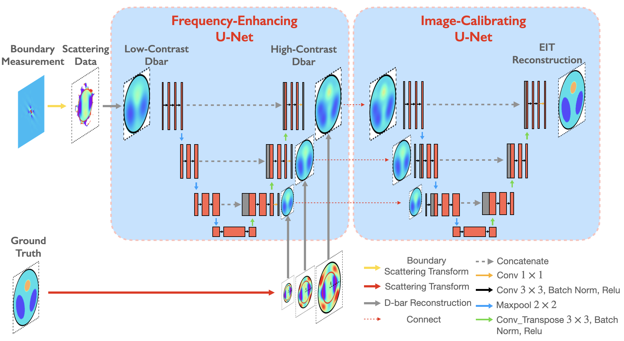
Figure 2: Our learning-based approach comprises two essential components: the frequency-enhancing U-net and the image-calibrating U-net. The frequency-enhancing U-net focuses on accentuating the contrast of the low-pass D-bar reconstructions by integrating high-frequency scattering information derived from ground truth data. Subsequently, the image-calibrating U-net leverages the prediction of the high-contrast D-bar image sequence at each level to generate the ultimate EIT reconstruction.

• Stage 1: Frequency Learning for Data Enhancement

  In the first stage, we consider utilizing the approximated high-frequency information obtained from the ground truth to enhance the low-contrast D-bar images. The target high-contrast D-bar images $\sigma_{R}(z)$ with increased truncation radius $R$ are generated by leveraging the scattering transformation (6) and the D-bar equation (13). From a numerical perspective, both the non-linear scattering transformation and the D-bar integral equations lack analytical closed-form solutions, necessitating the use of iterative algorithms for their solutions. However, its primary drawback is the requirement of point-wise execution for each $k$ and $z$, leading to time-consuming computations. To provide more clarity for the corresponding two remedies, we first utilize the asymptotic approximation $\mathbf{\tilde{t}}(k)$ to the complete scattering equation

  $$\mathbf{t}(k)\approx\mathbf{\tilde{t}}(k):=\int_{\Omega}q(z)e^{i(\bar{k}\bar{z}+kz)}dz,$$ (11)

  due to the asymptotic behavior of the CGO solution $\psi(z,k)\rightarrow e^{ikz}$ as $|k|\rightarrow\infty$. Eq.(11) can be computed parallelly for different $k$ without the need for solving numerical CGO solutions in advance. Subsequently, we define the truncated scattering data $\mathbf{t}_{R}(k)$ with the increased cutoff radius $R$ as follows:

  $$\mathbf{t}_{R}(k)=\begin{cases}\mathbf{t}^{\text{exp}}_{R^{\delta}}(k),&\text{ }|k|\leq R^{\delta}\\ \mathbf{\tilde{t}}(k),&\text{ }R^{\delta}<|k|\leq R\\ 0.&\text{ }|k|>R\end{cases}$$ (12)

  The second remedy is to accelerate the evaluation of the D-bar integral equations

  $$m_{R}(z,k)=1+\frac{1}{(2\pi)^{2}}\int_{|k^{\prime}|<R}\frac{\mathbf{t}_{R}\left(k^{\prime}\right)}{\left(k-k^{\prime}\right)\bar{k}^{\prime}}e^{-i(kz+\bar{k}\bar{z})}\overline{m_{R}\left(z,k^{\prime}\right)}dk^{\prime}$$ (13)

  using the surrogate GPU-based Richardson iterative method detailed in Subsection 4.3, and it finally yields the target frequency-enhanced images $\{\sigma^{(i)}_{R}\}_{i=1}^{N}\in\mathrm{R}^{W\times H}$. By concatenating the high-contrast D-bar approximations for $R\in\{R_{1},\cdots,R_{S}\}$, commonly selected as an arithmetic sequence, we can construct target frequency-enhanced image sequences denoted as $\{[\sigma^{(i)}_{R_{1}},\cdots,\sigma^{(i)}_{R_{S}}]\}_{i=1}^{N}\in\mathrm{R}^{S\times W\times H}$ for guided training.

• Stage 2: Image Domain Calibration for High-Quality Reconstruction

  Given the training pairs $\{(\sigma^{(i)}_{R^{\delta}},\sigma^{(i)})\}_{i=1}^{N}$ and the generated high-contrast D-bar image sequences $\{[\sigma^{(i)}_{R_{1}},\cdots,\sigma^{(i)}_{R_{S}}]\}_{i=1}^{N}$, we introduce a novel hybrid U-net-based network architecture. This architecture features two sequentially connected modified U-nets, each with a unique role in the EIT prediction process (see Fig.2). The first network $\mathbf{F}_{\Theta_{1}}(\cdot)$ is meticulously designed to predict the frequency-enhanced D-bar images, which aims to incorporate essential high-frequency information. For simplicity, we denote

  $$\mathbf{F}_{\Theta_{1}}(\sigma):=[\mathbf{F}^{(1)}_{\Theta_{1}}(\sigma),\cdots,\mathbf{F}^{(S)}_{\Theta_{1}}(\sigma)],$$

  where $\mathbf{F}^{(j)}_{\Theta_{1}}(\sigma)\in\mathrm{R}^{[W/2^{j-1}]\times[H/2^{j-1}]}$ represents the $j$-th downsampled output by adding a sub-branch to the commonly used U-net at the $j$-th level (see the left blue part of Fig.2). The second U-net $\mathbf{P}_{\Theta_{2}}(\cdot)$ plays a pivotal role in calibrating the predicted frequency-enhanced D-bar images. It unifies the information of D-bar images over varying resolutions, ultimately providing the predicted EIT reconstruction. Similarly, we have

  $$\mathbf{P}_{\Theta_{2}}(\mathbf{F}_{\Theta_{1}}(\sigma)):=\mathbf{P}_{\Theta_{2}}([\mathbf{F}^{(1)}_{\Theta_{1}}(\sigma),\cdots,\mathbf{F}^{(S)}_{\Theta_{1}}(\sigma)])\in\mathrm{R}^{H\times W},$$

  where $\mathbf{F}^{(j)}_{\Theta_{1}}(\sigma)$ is fed into the image-calibrating network at the $j$-th level by concatenating a sub-branch to the $j$-th level of the commonly used U-net (see the right blue part of Fig.2).

Specifically, we define the hybrid network as a composition of the frequency-enhancing network $\mathbf{F}_{\Theta_{1}}(\cdot)$ and the image-calibrating network $\mathbf{P}_{\Theta_{2}}(\cdot)$ with the combined supervised empirical loss:

$$\mathcal{L}(\Theta_{1},\Theta_{2}):=\alpha\sum\limits_{i=1}^{N}\sum\limits_{j=1}^{S}\|\mathbf{F}^{(j)}_{\Theta_{1}}(\sigma^{(i)}_{R^{\delta}})-\mathbf{D}^{j-1}(\sigma^{(i)}_{R_{j}})\|^{2}_{2}+\sum\limits_{i=1}^{N}\|\mathbf{P}_{\Theta_{2}}(\mathbf{F}_{\Theta_{1}}(\sigma^{(i)}_{R^{\delta}}))-\sigma^{(i)}\|^{2}_{2}$$ (14)

where $\mathbf{D}$ refers to the downsampling operator, and $\alpha$ is a constant weight for balancing two distinct loss terms (we find $\alpha=1$ performs well across our two datasets). It is noteworthy that our experiments reveal the superior generalization performance of the combined U-nets compared to a single U-net trained on data pairs only involving low-pass D-bar images and ground truths. To be specific, this approach excels in approximating conductivity values more precisely, effectively mitigating misleading artifacts in predictions, as indicated in Section 5. Thus, we think this hybrid framework could alleviate the complexity of this learning problem, which leverages the ground truth for the retrieval of high-frequency scattering information.

4 Numerical Implementations

In this section, we present our numerical implementations for the proposed hybrid learning scheme for the EIT reconstruction problem. Besides, the numerical implementation for the regularized D-bar method is provided in the book [4] (See Matlab code for computational resources). Note that we only utilize parts of synthetic conductivity phantoms generation, the simulated noisy Neumann-to-Dirichlet matrix $\mathbf{L}_{\sigma}^{\delta}$ and the computation of the truncated scattering data $\mathbf{t}^{\text{exp}}_{R^{\delta}}(k)$ in the non-linear frequency domain.

4.1 The Discrete Dirichlet-to-Neumann Map $\Lambda^{\delta}_{\sigma}$ Simulation

Trigonometric current patterns are considered to be applied on electrodes attached on the boundary, and the resulting voltages are solved for each electrode where the finite element method (FEM) is used for numerically computing EIT equations. Specifically, we firstly compute the Neumann-to-Dirichlet map $\mathcal{R}_{\sigma}$ using the sinusoidal basis functions:

$$\varphi_{n}(\theta)=\begin{cases}\frac{1}{\sqrt{\pi}}\sin(n\theta)&\text{ if }n<0\\ \frac{1}{\sqrt{\pi}}\cos(n\theta)&\text{ if }n>0\end{cases}$$ (15)

where $\varphi_{n}$ with $-N\leq n\leq N,n\neq 0$. The matrix representation $\mathbf{R}_{\sigma}=[\mathbf{R}_{\sigma}]_{2N\times 2N}$ for the NtoD map $\mathcal{R}_{\sigma}$ can be approximated by

$$(\mathbf{R}_{\sigma})_{m,n}=\langle\mathcal{R}_{\sigma}\varphi_{n},\varphi_{m}\rangle:=\int_{0}^{2\pi}(\mathcal{R}_{\sigma}\varphi_{n})(\theta)\varphi_{m}(\theta)d\theta$$ (16)

where $\mathcal{R}_{\sigma}\varphi_{n}=\left.u_{n}\right|_{\partial\Omega}$ with $\nabla\cdot\sigma\nabla u_{n}=0$ in $\Omega$, and the Neumann boundary condition $\left.\sigma\left(\frac{\partial u_{n}}{\partial\nu}\right)\right|_{\partial\Omega}=\phi_{n}$ on $\partial\Omega$. Further consider the boundary voltage data with additionally added relative Gaussian noise $\mathcal{N}_{n}$, which is the same as in [32]. In other words,

$$\mathcal{R}_{\sigma}^{\delta}\varphi_{n}=\mathcal{R}_{\sigma}\varphi_{n}+\delta\mathcal{N}_{n}\left\|\mathcal{R}_{\sigma}\varphi_{n}\right\|_{L^{\infty}}$$ (17)

where $\delta$ denotes the noise level of the simulated data, and $\mathcal{N}_{-N},...,\mathcal{N}_{N}$ are $2N$ independent noise samples from the standard Gaussian distribution. Finally, the noisy DtN matrix $\mathbf{L}_{\sigma}^{\delta}$ for approximating the DtN mapping $\Lambda^{\delta}_{\sigma}$ could be generated by inverting $\mathbf{R}_{\sigma}$ and adding a zero column and row to the middle of it as described in [4].

In this paper, totally $N=16$ different voltage patterns were applied to the boundary $\partial{\Omega}$ and the simulated noise levels $\delta=0,0.001,0.0075$ were considered for the noisy measurement matrices $[\mathbf{L}_{\sigma}^{\delta}]_{33\times 33}$. Then the corresponding truncated radius $R^{\delta}$ was individually set to be $6,5,4$ to guarantee the numerical stability in the $k$-space.

4.2 Evaluation of the Scattering Transformation and the D-bar Equations

The computational points for $\mathbf{t}^{\text{exp}}_{R^{\delta}}(k)$ and $\mathbf{t}_{[R^{\delta},R]}(k)$ were generated on $k$-vectors of $h=0.2$ equidistant points in the circle $|k|\leq{R^{\delta}}$ and the annulus ${R^{\delta}}<|k|<{R}$, respectively. The computation of the $\mathbf{t}^{\text{exp}}_{R^{\delta}}(k)$ was obtained from the numerical CGO solutions to $\psi(\cdot,k)$ in (5), which is referred to Chapter 15 of [4] for more implementation details. Furthermore, a $z$-grid of $269\times 269$ equidistributed $k$-points of the square $[-s,s)\times[-s,s)$ with $s=2.1$ was generated to discretize $q(z)$. To avoid singularities, the potential $q(z)$ was evaluated from the discontinuous conductivities $\sigma(z)$ with a slight Gaussian smoothing.

Meanwhile, the D-bar reconstruction requires the computational grids generated on a $k$-grid of $2^{l}\times 2^{l}$ equidistant points of the square $[-sR,sR)\times[-sR,sR)$ with $l=9$ and $s=2.1$, namely a $k$-grid discretization of size $512\times 512$. To be specific, for noisy measurements $\Lambda_{\sigma}^{\delta}$ the truncated radius $R^{\delta}$ will be used for the initial low-pass filtered reconstruction $\sigma_{R^{\delta}}$. Here, the scattering values defined in $|k|\leq{R^{\delta}}$ could be obtained by interpolation using the pre-computed $\mathbf{t}^{\text{exp}}_{R^{\delta}}(k)$ vectors while other points of $[-sR^{\delta},sR^{\delta})\times[-sR^{\delta},sR^{\delta})$ were padded with zeros. But for the high-pass frequency enhanced D-bar reconstruction $\sigma_{R}$ with the increased scattering radius $R$, the truncation radius $R$ was uniformly chosen to be $6,7,8$ numerically, which was selected to be an equidistant sequence. The lacked scattering data for ${R^{\delta}}<|k|<{R}$ was estimated through bilinear interpolation using the computed $\mathbf{t}_{[R^{\delta},R]}(k)$ vectors, and then the D-bar equations were solved based on the discretization of $[-sR,sR)\times[-sR,sR)$.

4.3 Parallel Computation for Solving the D-bar Equations

We mentioned that performing the inverse scattering transformation $\mathbf{t}^{-1}(z)$ is equivalent to solving the D-bar integral equation (13), which can be discretized into a complex-valued linear system parameterized by each $z$. Here, we turn to a classical matrix-free iterative technique, namely the Richardson iterative method, to solve the D-bar equations instead of the GMRES algorithm used in [4]. Specifically, the linear systems of the D-bar integral equations could be summarized as

$$[\mathbf{I}-\mathbf{A}(z,{\mathbf{t}_{R}})]\mathbf{m}_{R}(z,k)=\mathbb{1},$$ (18)

where $\mathbb{1}$ refers to the all-ones vector with the same size as $\mathbf{m}_{R}(z,k)\in R^{2^{2l+1}}$ and $\mathbf{A}(z,{\mathbf{t}_{R}})$ is the reduced linear operator which explicitly depends on the point $z$ and the scattering data $\mathbf{t}_{R}$. Rather than using the full matrix representation, the matrix-vector product of $\mathbf{A}(z,{\mathbf{t}_{R}})\mathbf{m}_{R}(z,k)$ could be efficiently evaluated via Fast Fourier Transform [4]. Therefore, we consider the following iterative scheme

$$\mathbf{m}^{(n+1)}_{R}=\mathbb{1}+\mathbf{A}\mathbf{m}^{(n)}_{R}$$ (19)

with initial guess $\mathbf{m}^{(0)}_{R}=\mathbb{1}$ for solving the numerical D-bar equations. Technically speaking, solving such D-bar equations for discrete $z$-grids could be extremely accelerated by GPU-based parallel computation, which is much faster than the original implementation in [4] using the GMRES algorithm on the CPU device. Here, we choose the maximal iteration number $N=5$ in the numerical implementations.

5 Numerical Results & Discussion

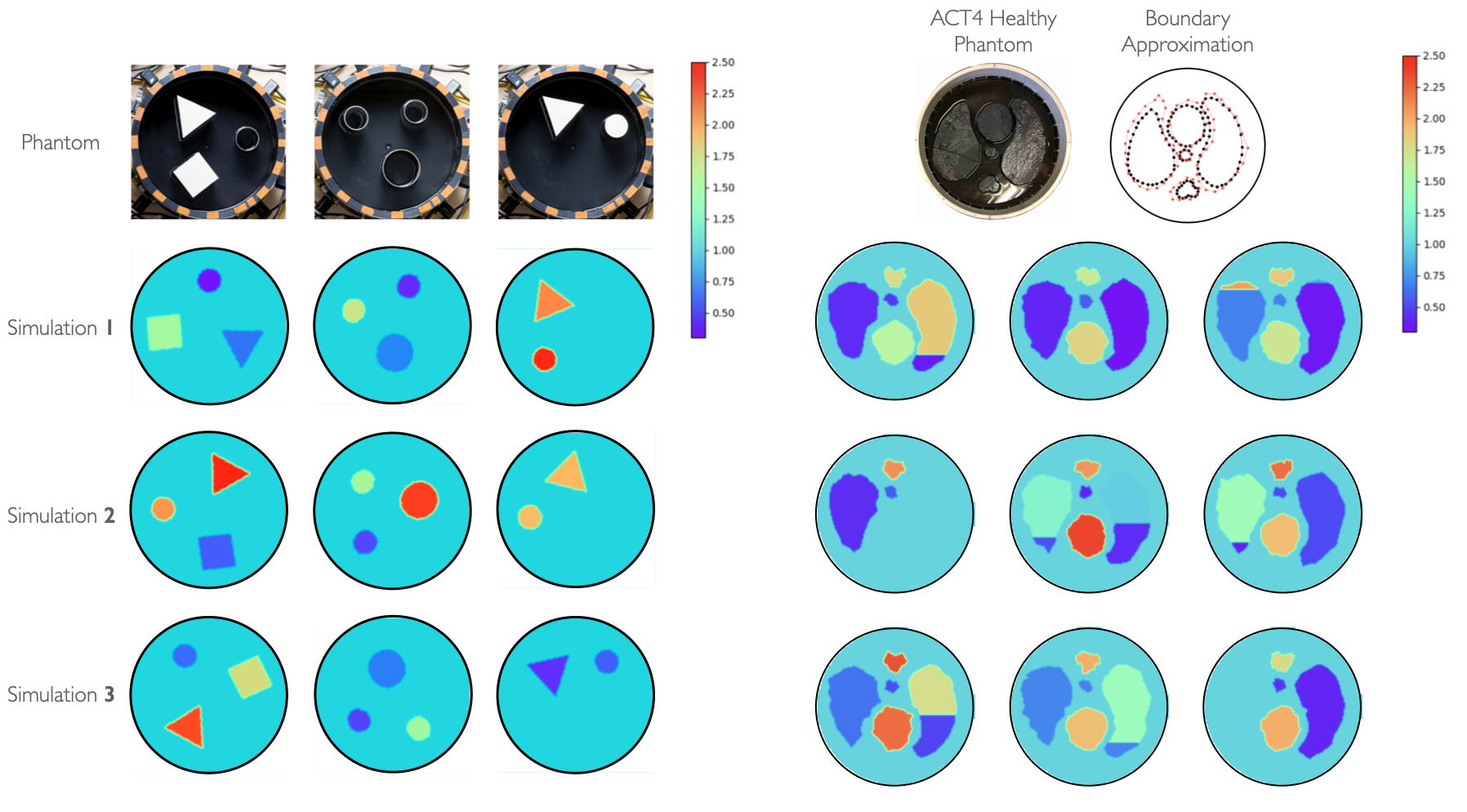
Figure 3: Several illustrative examples in KIT4 and ACT4 datasets

5.1 Data simulation for KIT4 and ACT4 datasets

The KIT4 dataset is a collection of simulated phantoms consisting of several discontinuous inclusions with some regular shapes. We first create randomly selected anomaly shapes and locations in the interior. The inclusions were not allowed to superimpose and then each one was assigned with an equal probability to be ’conductive’ or ’resistive’ for the background. Specifically, the values of the ’conductive’ parts and the ’resistive’ parts were sampled from the uniform distributions $[1.5,2.5]$ and $[0.3,0.7]$, respectively. The background’s value was always set to be $1$ which could be naturally extended to the outside of the circle. A total of $3280$ training samples and $820$ validation samples were simulated for each noise level $\delta$, and pairs of the truncated low-pass scattering data $\mathbf{t}^{\text{exp}}_{R^{\delta}}(k)$ and the ground truth $\sigma(z)$ were collected for training the neural network.

Meanwhile, the ACT4 dataset was created similarly to [26]. Using the ‘HLSA Healthy’ image shown in Fig.3 left top, we first manually extracted approximate organ boundaries and added a random Gaussian perturbation to the boundary points’ locations. Such simulated boundary shapes will not vary too greatly. Next, some organ injuries were also simulated by dividing both lungs into two portions with random-selected horizontal lines. Whether such injuries took place or not was determined by a given probability ($50\%$ chance). Besides, we randomly generate conductivity values in each of the above-divided portions from the uniform distribution $[0.3,2.5]$. Here, we simulated a total of 3200 samples for training and another 800 samples for validation. More simulations could be generated for better generalization ability but it was not considered in the scope of this study. See Fig.3 for both illustrative samples of the KIT4 dataset and the ACT4 dataset.

5.2 Reconstruction Results

We examine the reconstruction results of the proposed method on simulated testing data. The testing cases we explore are collected similarly, ensuring consistency with the distribution of the training data.

Fig.4 and Fig.5 illustrate our algorithm’s workflow for the KIT4 and ACT4 datasets. Each column of these figures depicts the processed images, starting with the corresponding ground truth $\sigma(z)$ and culminating in the final network prediction $\tilde{\sigma}(z)$ for each sample. Notably, the second and third images in both figures showcase the low-pass D-bar reconstructions $\sigma_{R^{\delta}}(z)$ and the enhanced D-bar prediction $\sigma_{R}(z)$ with high contrast, respectively. Our method consistently delivers gradual improvements in visual quality throughout the reconstruction process. Impressively, the U-net architecture reliably predicts the $\sigma_{R_{j}}(z)$ sequence, demonstrating a significantly lower validation loss compared to the direct prediction of the ground truth. This might be attributed to the high similarity between the D-bar solutions $\sigma_{R^{\delta}}(z)$ and $\sigma_{R}(z)$.

Furthermore, the image-calibrating U-net plays a crucial role as a module for post-processing, enabling the generation of reconstructions with distinct boundaries for isolated inclusions. In contrast to conventional approaches that post-process low-contrast D-bar reconstructions, it utilizes the predicted high-contrast D-bar sequence as input at each resolution level. Compared to the Deep D-bar method introduced in [26], the numerical experiments reveal that our trained module exhibits reduced susceptibility to over- or under-estimation of conductivity values within separate regions. Moreover, it effectively mitigates misleading artifacts that could potentially compromise the accuracy of the final reconstruction. Numerical results demonstrate the significance of our hybrid multi-scale structure with substantial improvements as depicted in Fig.4 and Fig.5, as well as in the overall quantitative results discussed in the next subsection.

	Sample 1	Sample 2	Sample 3	Sample 4	Sample 5	Sample 6	Sample 7

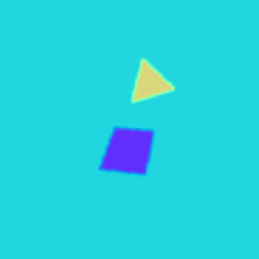
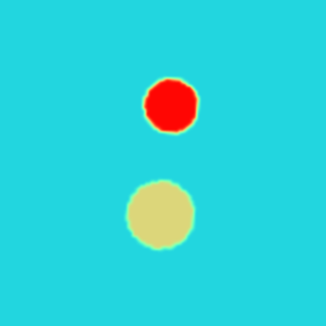
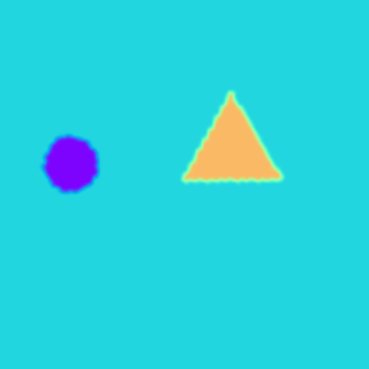
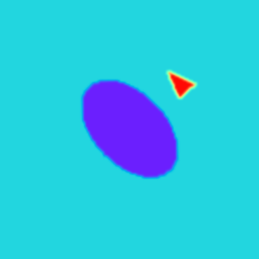
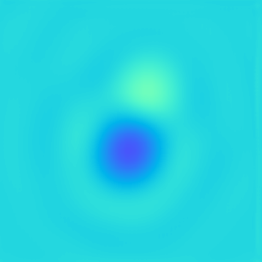
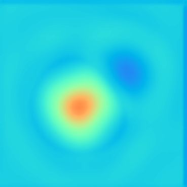
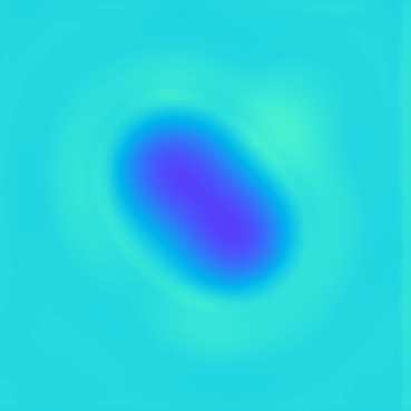
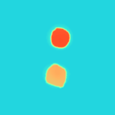
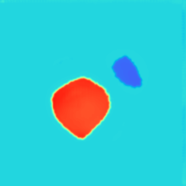
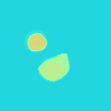
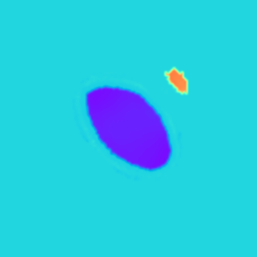
Figure 4: The figure depicts the predicted images during the reconstruction process of the proposed framework for KIT4 dataset.

	Sample 1	Sample 2	Sample 3	Sample 4	Sample 5	Sample 6	Sample 7

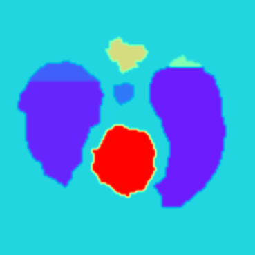
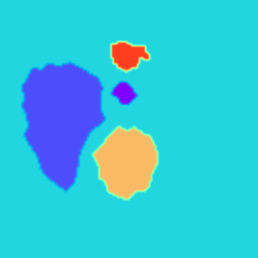
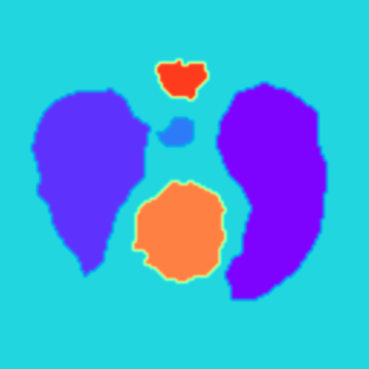
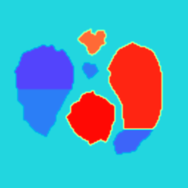
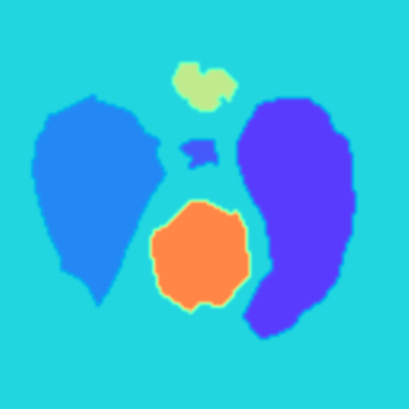
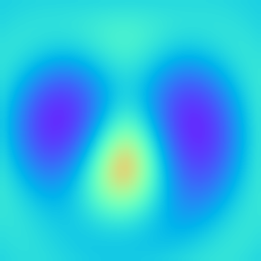
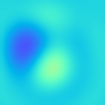
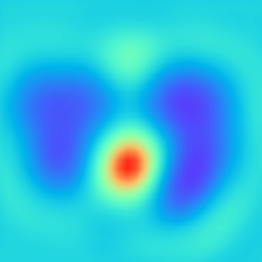
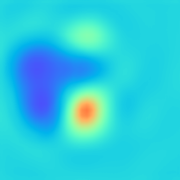
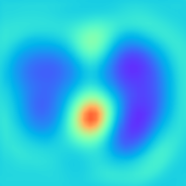
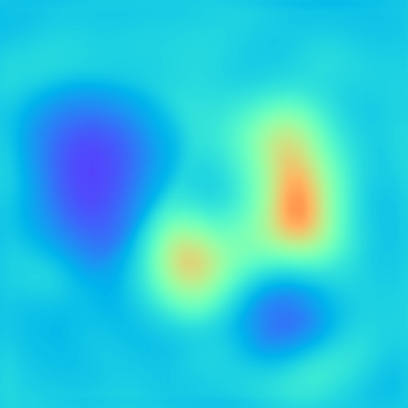
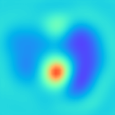
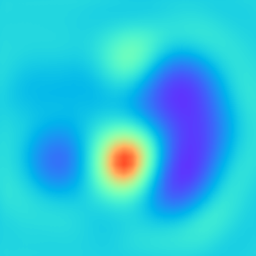
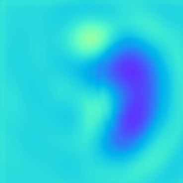
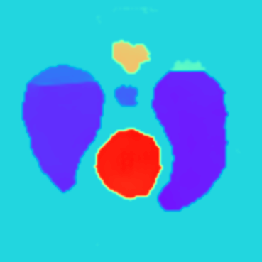
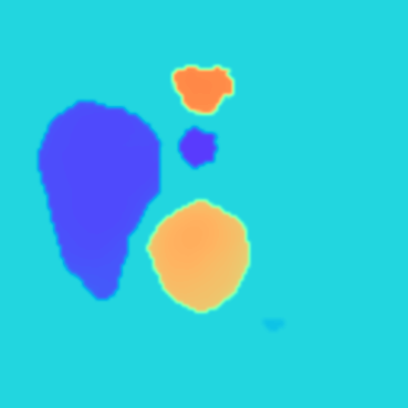
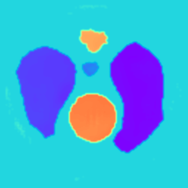
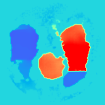
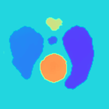
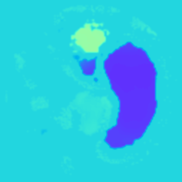
Figure 5: The figure depicts the predicted images during the reconstruction process of the proposed framework for ACT4 dataset.

5.3 Comparison Results

In this research, we choose three commonly used metrics including PSNR (Peak Signal-to-Noise Ratio), SSIM (Structural Similarity Indices), and RMSE (Relative Mean Square Error) for quality assessment. The higher values of both PSNR and SSIM and the lower RMSE indicate more satisfactory reconstruction results. Besides, our proposed method will be compared with three supervised learning-based methods: (1) CNN [33] (2) Deep D-bar [26] (3) TSDL [34] and two non-learning methods: (1) NOSER [35] (2) D-bar [4].

Fig.6 and Fig.7 shows a visual comparison of numerical results for KIT4 and ACT4 datasets. It can be seen that our deep learning method noticeably outperformed two non-learning methods: NOSER and D-bar methods. The NOSER algorithm [35] is an iterative-based optimization method for minimizing the PDE-based boundary misfit. Such a method typically suffers from high computational complexity because it requires computing the Jacobian of the measurement change to the conductivity change repetitively. However, the evaluation of the hybrid U-nets in our method is highly computationally efficient on GPUs, and the D-bar reconstruction could be also significantly accelerated as introduced in Subsection 4.3. Hence, our method is expected to be real-time capable of EIT reconstruction.

Compared to other supervised-based learning methods, the proposed method also shows much superior performance both visually and quantitatively. The CNN-based learning method in [33] directly approximated the mapping from measurements $\mathbf{L}_{\sigma}^{\delta}$ to corresponding ground truths $\sigma(z)$. But this direct-mapping-based neural network seemed to have poor generalization ability and only the negative parts could be reconstructed in the fifth column of Fig.6 and Fig.7. The TSDL method in [34] owns a trainable pre-reconstruction stage and a post-processing stage. Its first stage back-projects the measurements to the image space and then the CNN is used for improving the pre-reconstructed images. The ACT4 experiment in the fourth column of Fig.7 demonstrates the effectiveness of the method for reconstructing such organs’ phantoms, but the method is prone to produce lots of unexpected artifacts in the KIT4 experiment in Fig.6. It could be seen that our proposed method not only significantly reduces the misleading artifacts and keeps the sharp division for each isolated inclusion but also works well for both the shape reconstruction and the conductivity estimation.

	Ground truth	NOSER[35]	Dbar[4]	CNN-based [36]	TSDL[34]	Deep-Dbar[26]	Ours

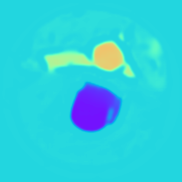
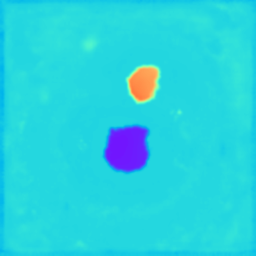
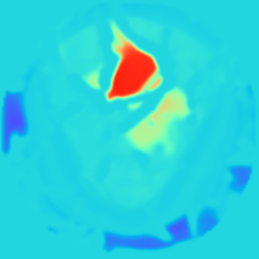
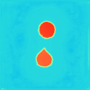
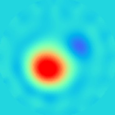
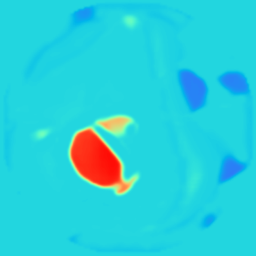
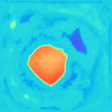
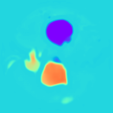
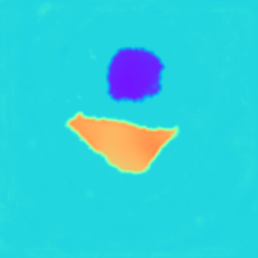
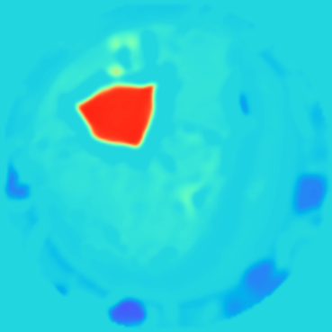
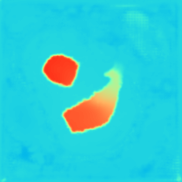
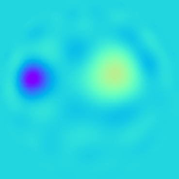
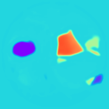
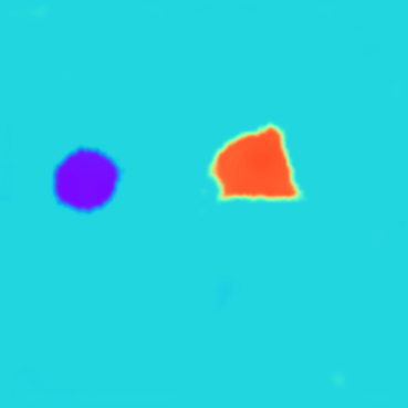
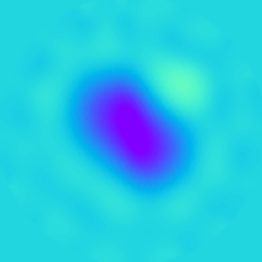
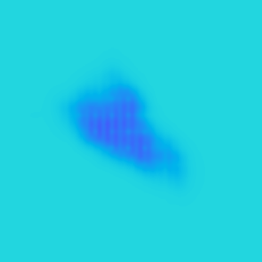
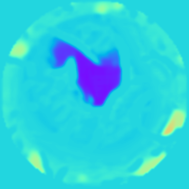
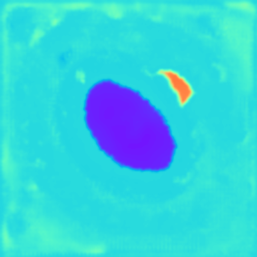
Figure 6: Each row depicts the corresponding ground truth and reconstruction results produced by comparison methods and ours for each KIT4 samples.

	Ground truth	NOSER[35]	D-bar[4]	CNN-based [36]	TSDL[34]	Deep D-bar[26]	Ours

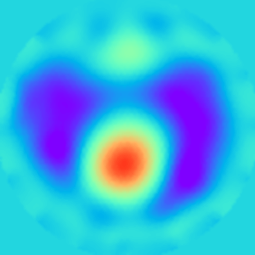
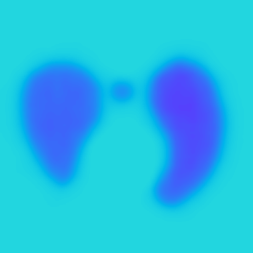
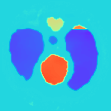
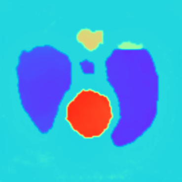
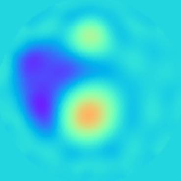
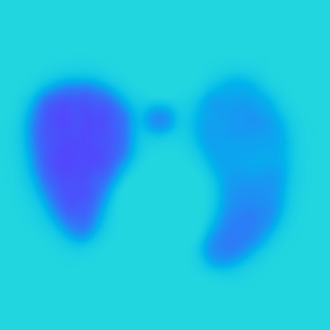
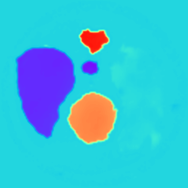
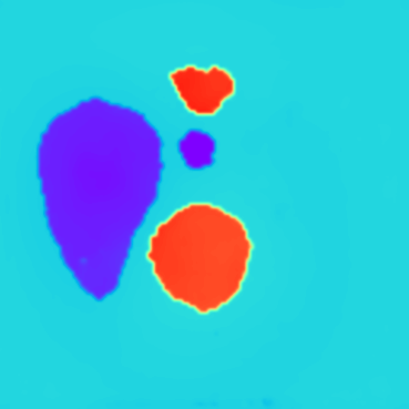
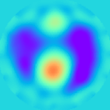
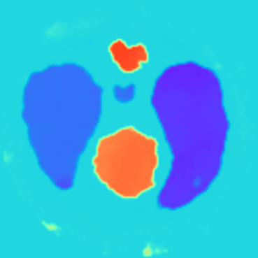
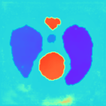
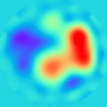
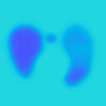
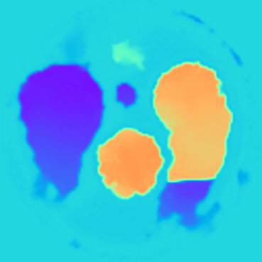
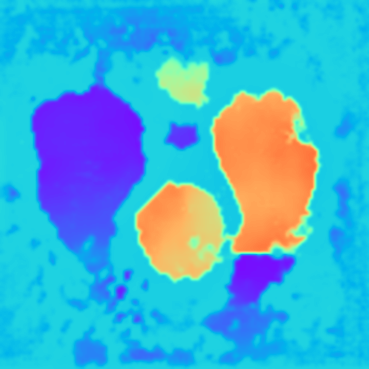
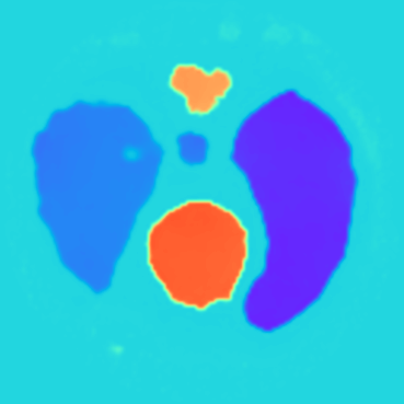
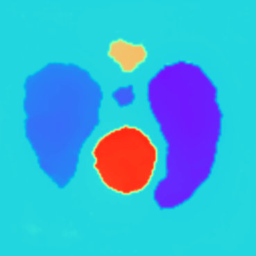
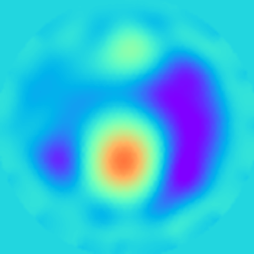
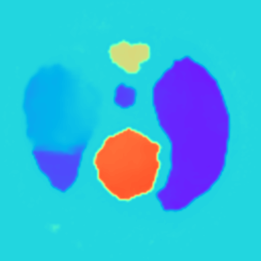
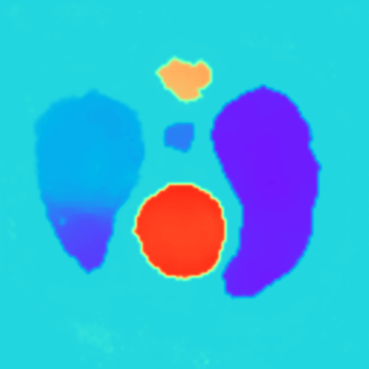
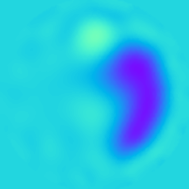
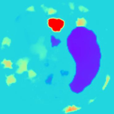
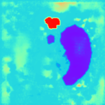
Figure 7: Each row depicts the corresponding ground truth and reconstruction results produced by comparison methods and ours for each ACT4 samples.

datasets	Metrics	Noise Levels	NOSER	D-bar	CNN	TSDL	Deep D-bar	Ours
KIT4	PSNR$\uparrow$	$0.75\%$	24.33	21.04	20.21	23.68	24.75	25.60
		$0.1\%$	26.70	24.22	22.41	24.56	25.78	27.67
		$0\%$	27.15	25.65	23.16	26.12	26.97	28.89
	SSIM$\uparrow$	$0.75\%$	0.8165	0.7692	0.8025	0.8419	0.8855	0.9235
		$0.1\%$	0.8396	0.7703	0.8065	0.8742	0.9134	0.9341
		$0\%$	0.8714	0.8020	0.8109	0.8902	0.9176	0.9455
	RMSE$\downarrow$	$0.75\%$	0.1136	0.1521	0.2018	0.1742	0.1213	0.1096
		$0.1\%$	0.0868	0.1376	0.1998	0.1446	0.1021	0.0812
		$0\%$	0.0740	0.1143	0.1832	0.1321	0.0988	0.0694
ACT4	PSNR$\uparrow$	$0.75\%$	22.44	19.19	17.33	23.24	22.62	23.63
		$0.1\%$	23.12	20.90	18.02	24.68	23.57	25.04
		$0\%$	24.46	22.89	18.41	25.34	24.43	26.61
	SSIM$\uparrow$	$0.75\%$	0.6877	0.6556	0.7533	0.8291	0.7949	0.8172
		$0.1\%$	0.7212	0.6754	0.7643	0.8457	0.8214	0.8521
		$0\%$	0.7315	0.6851	0.7706	0.8720	0.8326	0.8657
	RMSE$\downarrow$	$0.75\%$	0.1588	0.2382	0.2909	0.1468	0.1578	0.1445
		$0.1\%$	0.1321	0.2106	0.2743	0.1280	0.1499	0.1223
		$0\%$	0.1286	0.2047	0.2757	0.1193	0.1282	0.1049

Table 1: Quantitative comparison for KIT4 and ACT4 datasets to PSNR, SSIM and RMSE metrics

5.4 Computational Efficiency

Another key motivation is that we hope the proposed method could share the advantages of the direct methods in terms of computational efficiency. To provide a comprehensive comparison, see Table 2 for the comparison of different methods on training/testing time.

	NOSER [35]	D-bar [4]	TSDL [34]	Deep D-bar [26]	Ours
Training Time	—	—	40min	40min	1h
Testing Time	305.02s	54.86s	10.47s	3.95s	4.43s

Table 2: Comparison of training/testing time for different methods

The NOSER algorithm requires solving the non-linear PDE systems and the linear adjoint equations recursively for different boundary conditions, therefore its computational demand is typically higher than other direct methods. TSDL follows the difference imaging strategy which also needs the computation of the Jacobian and large matrix inversion. The D-bar method resorts to solving D-bar integral equations instead of PDEs. Here, the original D-bar method uses the CPU-based GMRES iterative algorithm for solving D-bar equations, while the Deep D-bar method and the proposed method will use the GPU-based Richardson iterative algorithm to obtain real-time D-bar reconstructions.

Here, all non-linear PDE solvers are executed on the Intel-Xeon-Platinum-8358P CPU, while the training and inference processes of deep learning part and GPU-based Richardson D-bar solvers are performed on NVIDIA-A100 GPU.

6 Ablation Study

The ablation study is aimed to evaluate the numerical performance gain brought by introducing the multi-scale structure. Here, the multi-scale structure means that the frequency-enhancing U-net predicts a sequence of high-contrast D-bar images for different truncation radii, while the U-net with the single-scale structure only predicts one high-contrast D-bar image for a fixed truncation radius in the non-linear scattering domain. The whole experiment is conducted on the ACT4 dataset with three simulated noise levels $\delta=0\%,0.1\%,0.75\%$, we consider the truncation radii $R^{\delta}=4,5,6$ for each noise level, respectively. It can be seen from Table 3 that the proposed method for various measurement noise levels has uniformly lower reconstruction errors compared to the single-scale structure, which demonstrates the effectiveness of the introduced multi-scale structure for predicting frequency-enhanced D-bar sequences.

Noise Levels		$\delta=0.75\%$		$\delta=0.1\%$		$\delta=0\%$
		Multi-scale	Single-scale	Multi-scale	Single-scale	Multi-scale	Single-scale
Metrics	PSNR $\uparrow$	23.63	22.94	25.04	23.78	26.61	24.80
	SSIM $\uparrow$	0.8172	0.7839	0.8521	0.8235	0.8657	0.8481
	RMSE $\downarrow$	0.1445	0.1543	0.1223	0.1355	0.1049	0.1291

Table 3: Comparison of the reconstruction quality for different U-net structures

7 Conclusions

To overcome the limitation of the regularized D-bar method, we introduce a novel approach that combines a multi-scale neural network architecture with the widely adopted U-net framework. This innovative combination allows us to retrieve D-bar image sequences, progressively enhancing conductivity contrast from low to high resolutions. Our results demonstrate the superiority of the multi-scale structure over other approaches, in effectively reducing artifacts and refining the quality of conductivity approximations.

Furthermore, we recognize the computational complexity associated with solving discrete D-bar systems using the GMRES algorithm, particularly on CPU-based devices. To address this issue, we develop a GPU-based Richardson iterative method, significantly accelerating the D-bar reconstruction process. Through extensive numerical experiments, conducted on simulated EIT data from the KIT4 and ACT4 systems, we have showcased substantial improvements in absolute EIT imaging quality compared to existing methodologies. These findings underscore the potential of our proposed approach in advancing the field of EIT, offering more accurate and high-quality conductivity reconstructions.

References

- [1] Andy Adler and David Holder. Electrical impedance tomography: methods, history and applications. CRC Press, 2021.
- [2] Trevor A York. Status of electrical tomography in industrial applications. Journal of Electronic imaging, 10(3):608–619, 2001.
- [3] A Abubakar, TM Habashy, M Li, and J Liu. Inversion algorithms for large-scale geophysical electromagnetic measurements. Inverse Problems, 25(12):123012, 2009.
- [4] Jennifer L Mueller and Samuli Siltanen. Linear and nonlinear inverse problems with practical applications. SIAM, 2012.
- [5] Adrian I Nachman. Global uniqueness for a two-dimensional inverse boundary value problem. Annals of Mathematicmas, pages 71–96, 1996.
- [6] Zhou Zhou, Gustavo Sato dos Santos, Thomas Dowrick, James Avery, Zhaolin Sun, Hui Xu, and David S Holder. Comparison of total variation algorithms for electrical impedance tomography. Physiological measurement, 36(6):1193, 2015.
- [7] Bangti Jin, Yifeng Xu, and Jun Zou. A convergent adaptive finite element method for electrical impedance tomography. IMA Journal of Numerical Analysis, 37(3):1520–1550, 2017.
- [8] Bangti Jin, Taufiquar Khan, and Peter Maass. A reconstruction algorithm for electrical impedance tomography based on sparsity regularization. International Journal for Numerical Methods in Engineering, 89(3):337–353, 2012.
- [9] Md Rabiul Islam and Md Adnan Kiber. Electrical impedance tomography imaging using gauss-newton algorithm. In 2014 International Conference on Informatics, Electronics & Vision (ICIEV), pages 1–4. IEEE, 2014.
- [10] Rick Hao Tan and Carlos Rossa. Electrical impedance tomography using differential evolution integrated with a modified newton raphson algorithm. In 2020 IEEE International Conference on Systems, Man, and Cybernetics (SMC), pages 2528–2534. IEEE, 2020.
- [11] Tony F Chan and Xue-Cheng Tai. Level set and total variation regularization for elliptic inverse problems with discontinuous coefficients. Journal of Computational Physics, 193(1):40–66, 2004.
- [12] Eric T Chung, Tony F Chan, and Xue-Cheng Tai. Electrical impedance tomography using level set representation and total variational regularization. Journal of computational physics, 205(1):357–372, 2005.
- [13] X-D Chen. Subspace-based optimization method in electric impedance tomography. Journal of Electromagnetic Waves and Applications, 23(11-12):1397–1406, 2009.
- [14] Zhun Wei, Rui Chen, Hongkai Zhao, and Xudong Chen. Two fft subspace-based optimization methods for electrical impedance tomography. Progress In Electromagnetics Research, 157:111–120, 2016.
- [15] P Wang, JS Lin, and M Wang. An image reconstruction algorithm for electrical capacitance tomography based on simulated annealing particle swarm optimization. Journal of applied research and technology, 13(2):197–204, 2015.
- [16] Zhun Wei, Dong Liu, and Xudong Chen. Dominant-current deep learning scheme for electrical impedance tomography. IEEE Transactions on Biomedical Engineering, 66(9):2546–2555, 2019.
- [17] Andreas Kirsch and Natalia Grinberg. The factorization method for inverse problems, volume 36. OUP Oxford, 2007.
- [18] Isaac Harris. Regularization of the factorization method with applications to inverse scattering. arXiv preprint arXiv:2202.13411, 2022.
- [19] Yat Tin Chow, Kazufumi Ito, and Jun Zou. A direct sampling method for electrical impedance tomography. Inverse Problems, 30(9):095003, 2014.
- [20] Masaru Ikehata. Reconstruction of the support function for inclusion from boundary measurements. Journal of Inverse and Ill-Posed Problems, 8(4):367–378, 2000.
- [21] David Isaacson, Jennifer L Mueller, Jonathan C Newell, and Samuli Siltanen. Reconstructions of chest phantoms by the d-bar method for electrical impedance tomography. IEEE Transactions on medical imaging, 23(7):821–828, 2004.
- [22] Dong Liu, Junwu Wang, Qianxue Shan, Danny Smyl, Jiansong Deng, and Jiangfeng Du. Deepeit: deep image prior enabled electrical impedance tomography. IEEE Transactions on Pattern Analysis and Machine Intelligence, 2023.
- [23] Yuwei Fan and Lexing Ying. Solving electrical impedance tomography with deep learning. Journal of Computational Physics, 404:109119, 2020.
- [24] Yuwei Fan, Cindy Orozco Bohorquez, and Lexing Ying. Bcr-net: A neural network based on the nonstandard wavelet form. Journal of Computational Physics, 384:1–15, 2019.
- [25] Ruchi Guo and Jiahua Jiang. Construct deep neural networks based on direct sampling methods for solving electrical impedance tomography. SIAM Journal on Scientific Computing, 43(3):B678–B711, 2021.
- [26] Sarah Jane Hamilton and Andreas Hauptmann. Deep d-bar: Real-time electrical impedance tomography imaging with deep neural networks. IEEE transactions on medical imaging, 37(10):2367–2377, 2018.
- [27] Sarah J Hamilton, Asko Hänninen, Andreas Hauptmann, and Ville Kolehmainen. Beltrami-net: domain-independent deep d-bar learning for absolute imaging with electrical impedance tomography (a-eit). Physiological measurement, 40(7):074002, 2019.
- [28] Guixian Xu, Huihui Wang, and Qingping Zhou. Enhancing electrical impedance tomography reconstruction using learned half-quadratic splitting networks with anderson acceleration. arXiv preprint arXiv:2304.14491, 2023.
- [29] Maziar Raissi, Paris Perdikaris, and George E Karniadakis. Physics-informed neural networks: A deep learning framework for solving forward and inverse problems involving nonlinear partial differential equations. Journal of Computational physics, 378:686–707, 2019.
- [30] Leah Bar and Nir Sochen. Unsupervised deep learning algorithm for pde-based forward and inverse problems. arXiv preprint arXiv:1904.05417, 2019.
- [31] Olaf Ronneberger, Philipp Fischer, and Thomas Brox. U-net: Convolutional networks for biomedical image segmentation. In Medical Image Computing and Computer-Assisted Intervention–MICCAI 2015: 18th International Conference, Munich, Germany, October 5-9, 2015, Proceedings, Part III 18, pages 234–241. Springer, 2015.
- [32] Sarah J Hamilton, Juan Manuel Reyes, Samuli Siltanen, and Xiaoqun Zhang. A hybrid segmentation and d-bar method for electrical impedance tomography. SIAM Journal on Imaging Sciences, 9(2):770–793, 2016.
- [33] Delin Hu, Keming Lu, and Yunjie Yang. Image reconstruction for electrical impedance tomography based on spatial invariant feature maps and convolutional neural network. In 2019 IEEE International Conference on Imaging Systems and Techniques (IST), pages 1–6. IEEE, 2019.
- [34] Shangjie Ren, Kai Sun, Chao Tan, and Feng Dong. A two-stage deep learning method for robust shape reconstruction with electrical impedance tomography. IEEE Transactions on Instrumentation and Measurement, 69(7):4887–4897, 2019.
- [35] Margaret Cheney, David Isaacson, and Jonathan C. Newell. Electrical impedance tomography. SIAM Review, 41(1):85–101, 1999.
- [36] Akarsh Pokkunuru, Amirmohmmad Rooshenas, Thilo Strauss, Anuj Abhishek, and Taufiquar Khan. Improved training of physics-informed neural networks using energy-based priors: a study on electrical impedance tomography. In International Conference on Learning Representations, 2023.