Anole: Adapting Diverse Compressed Models for Cross-scene Prediction on Mobile Devices

Abstract

Emerging Artificial Intelligence of Things (AIoT) applications desire online prediction using deep neural network (DNN) models on mobile devices. However, due to the movement of devices, unfamiliar test samples constantly appear, significantly affecting the prediction accuracy of a pre-trained DNN. In addition, unstable network connection calls for local model inference. In this paper, we propose a light-weight scheme, called Anole, to cope with the local DNN model inference on mobile devices. The core idea of Anole is to first establish an army of compact DNN models, and then adaptively select the model fitting the current test sample best for online inference. The key is to automatically identify model-friendly scenes for training scene-specific DNN models. To this end, we design a weakly-supervised scene representation learning algorithm by combining both human heuristics and feature similarity in separating scenes. Moreover, we further train a model classifier to predict the best-fit scene-specific DNN model for each test sample. We implement Anole on different types of mobile devices and conduct extensive trace-driven and real-world experiments based on unmanned aerial vehicles (UAVs). The results demonstrate that Anole outwits the method of using a versatile large DNN in terms of prediction accuracy (4.5% higher), response time (33.1% faster) and power consumption (45.1% lower).

I Introduction

Motivation. Last decade has witnessed the booming development of Artificial Intelligence of Things (AIoT), an emerging computing paradigm that marries artificial intelligence (AI) and Internet of Things (IoT) technologies to enable independent decision-making at each component level of the interconnected system. In many AIoT scenarios, deep neural network (DNN) model inference (i.e., prediction) tasks are required to execute on mobile devices, referred to as the online mobile inference (OMI) problem, with stringent accuracy and latency requirements. For example, unmanned aerial vehicles (UAVs) need to constantly detect surrounding objects in real time [1]; a dash cam mounted on a vehicle needs to perform continuous image object detection [2]; robots in smart factories need to detect objects in production lines in real time, and interact with human workers and other robots [3].

To address the OMI problem, however, is demanding for two reasons as follows. First, given that mobile devices constantly experience scene changes while moving (e.g., due to various lighting conditions, weather conditions, and viewing angles), the output of DNNs should remain reliable and accurate. Training a statistical learning DNN on a given dataset, as in normal deep learning paradigm, becomes difficult to guarantee the robustness, interpretability and correctness of the output of the statistical learning models when data samples are out-of-distribution (OOD) [4]. Second, the response time for model inference should satisfy a rigid delay budget to support real-time interactions with these devices. As mobile devices are resource-constrained in terms of computation, storage and energy, they cannot handle large DNNs. Though it would be beneficial to offload a part of or even entire inference tasks to a remote cloud, unstable communication between mobile devices and the cloud may lead to unpredictable delay.

In the literature, much effort has been made to improve DNN model inference accuracy on mobile devices but in static scenarios. One main branch aims to develop DNNs specially designed for mobile devices [5, 6, 7, 8] or to compress (e.g., via model pruning and quantization) existing DNNs to match the computing capability of a mobile device [9, 10]. Such schemes ensure real-time model inference at the expense of compromised accuracy, especially when dealing with OOD data samples. Another branch is to divide DNNs and perform collaborative inference on both edge devices and the cloud [11, 12, 13], or to transmit compressed sensory data to the cloud for data recovery and model inference [14, 15]. These approaches need coordination with the cloud for each inference, leading to unpredictable inference delays when the communication link is unstable or disconnected. As a result, to the best of our knowledge, there is no successful solution to the OMI problem yet.

Our approach. We propose Anole, which enables online model inference on mobile devices in dynamic scenes. We have the insight that a compressed DNN targeted for a particular scene (i.e., data distribution) can achieve comparable inference accuracy provided by a fully-fledged large DNN. The core idea of Anole is to first establish a colony of compressed scene-specific DNNs, and then adaptively select the model best suiting the current test sample for online inference. To this end, it is essential to identify scenes from the perspective of DNN models. We design a weakly-supervised scene representation learning scheme by combining both human heuristics and feature similarity in separating scenes. After that, for each identified scene, an individual compressed DNN model can be trained. Furthermore, we train a model classifier to predict the best-fit compressed DNN models for use during online inference. As a result, compelling prediction accuracy can be achieved on mobile devices by actively recruiting most capable compressed models, without any intervention with the cloud.

Challenges and contributions. The Anole design faces three main challenges. First, how to obtain model-friendly scenes and train scene-specific DNNs from public datasets is unclear, as the distribution that a DNN model can characterize is implicit. One naive way is to use semantic attributes (e.g., time, location, weather and light conditions) of data to define scenes of similar data samples. However, as shown in our empirical study, DNNs trained on such scenes cannot reach satisfactory prediction accuracy even on their respective training scenes. To tackle this challenge, we design a scene representation learning algorithm that combines semantic similarity and feature similarity of data to filter out scenes. Specifically, human heuristic is first used to define scenes of similar semantic attribute values, referred to as semantic scenes. Then, a scene representation model, denoted as $\mathcal{M}_{scene}$, is trained using the indices of semantic scenes as labels. After that, we can obtain embeddings of all data samples extracted with $\mathcal{M}_{scene}$ and believe such embeddings can well characterize semantic information. Therefore, by conducting multi-granularity clustering on these embeddings, we can obtain clusters of data samples with similar semantic information in feature space, referred to as model-friendly scenes. Finally, a compressed DNN can be trained on each model-friendly scene, constituting a model repository for use.

Second, given a test sample, how to determine the best-fit models or whether such models even exist in the model repository is hard to tell. To deal with this challenge, we train a model classifier, denoted as $\mathcal{M}_{decision}$, to predict the best model for use. Specifically, for each model-friendly scene, we select those data samples in the scene that can be accurately predicted by the corresponding DNN and use the index of the DNN as the label to train $\mathcal{M}_{decision}$. Instead of testing all data samples, we use Thompson sampling to establish balanced training sets at a low computational cost. With a well-trained $\mathcal{M}_{decision}$, the most suitable compressed models can be predicted and the prediction confidence can be used to indicate whether such models exist.

Last, how to deploy those pre-trained compressed DNNs on mobile devices with constrained memory is non-trivial. We have the observation that the utility of models follows a power-law distribution over all test videos. This implies that it is feasible to cache a small number of most frequently used compressed models and take a least frequently used (LFU) model replacement strategy.

We implement Anole on three typical mobile devices, i.e., Jetson Nano, Jetson TX2 NX and a laptop, with each equipped with a CPU/MCU and an entry-level GPU, to conduct the image object detection task on moving vehicles. Specifically, we train the $\mathcal{M}_{scene}$ based on Resnet18 [16], a pack of 19 compressed DNNs based on YOLOv3-tiny [17], and the $\mathcal{M}_{decision}$ based on Resnet18 accordingly, using three driving video datasets collected from multiple cities in different counties. We conduct extensive trace-driven and real-world experiments using UAVs. Results demonstrate that Anole is lightweight and agile to switch best models with low latencies of 61.0 ms, 13.9 ms, and 52.0 ms on Jetson Nano, Jetson TX2 NX, and the laptop, respectively. In cross-scene (i.e., seen but fast-changing scenes) setting, Anole can achieve a high F1 prediction accuracy of 56.4% whereas the F1 score of a general large DNN model and a general compact DNN are 50.7% and 45.9%, respectively. In hard new-scene (i.e., unseen scenes) setting, Anole can maintain a high F1 score of 48.7% whereas the F1 score of the general large DNN and the general compact DNN drops to 46.6% and 41.1%, respectively.

We highlight the main contributions made in this paper as follows: 1) A new solution to the OMI problem by recruiting a pack of compact but specialized models on resource-constrained mobile devices, without any intervention with the cloud during online model inference; 2) A scene partition method that effectively facilitates the training of specialized models by leveraging both semantic and feature similarity of the data; 3) We have implemented Anole on typical mobile devices and conducted extensive trace-driven and real-world experiments, the results of which demonstrate the efficacy of Anole.

II Problem Definition

II-A System Model

We consider three types of entities in the system:

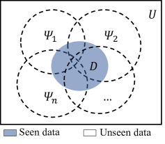
Figure 1: Illustration of the online mobile inference problem, where data distributions characterized by statistical models (depicted as dashed disks) are implicit and not easy to understand.

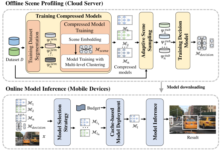
Figure 2: System architecture of Anole, which consists of the offline scene profiling on cloud servers and the online model inference on mobile devices. Communication between both parts is carried out offline.

• Mobile devices: Mobile devices have constrained computational power and a limited amount of memory but are affordable for running and storing compressed DNNs. Such devices may be moving while performing online inference tasks at the same time. They are battery-powered, desiring lightweight operations. In addition, they can communicate with a cloud server via an unstable wireless network connection for offline model training and downloading.

• Cloud server: A cloud server has sufficient computational power and storage for offline model training. During online inference, the cloud server is not involved.

• Complex environment: We consider practical environments where background objects and light conditions have distinct spatial and temporal distributions. When mobile devices move in such a complex environment, they constantly experience fast scene changes.

II-B Problem Formulation

Given the set of all available labeled data, denoted as $D$, a compressed DNN model, denoted as $\mathcal{M}_{i}$, can be trained on a particular dataset, denoted as $\Gamma_{i}$, which is a subset of $D$, i.e., $\Gamma_{i}\subseteq D$ for $i\in\mathbb{N}$. For instance, $\Gamma_{i}$ can be established based on some semantic attributes of data. Assume that a set of $n$ models $\{\mathcal{M}_{1},\mathcal{M}_{2},\cdots,\mathcal{M}_{n}\}$ have been pre-trained on respective training datasets $\{\Gamma_{1},\Gamma_{2},\cdots,\Gamma_{n}\}$ and the implicit data distributions that those models can characterize are $\{\Psi_{1},\Psi_{2},\cdots,\Psi_{n}\}$, respectively, which means that if a data sample $x\in\Psi_{i}$ for $i\in[1,n]$, model $\mathcal{M}_{i}$ guarantees to output accurate prediction for $x$. We have the following proposition:

Proposition 1.

Though $\mathcal{M}_{i}$ is trained on $\Gamma_{i}$, not all data samples in $\Gamma_{i}$ necessarily belong to $\Psi_{i}$, i.e., $\Gamma_{i}\not\subset\Psi_{i}$.

As illustrated in Figure 1, given $D$, we can train such a set of $n$ models $M=\{\mathcal{M}_{1},\mathcal{M}_{2},\cdots,\mathcal{M}_{n}\}$ so that $D\subset\bigcup_{i=1}^{n}\Psi_{i}$. As in mobile settings, any data sample $x\in U$ can be encountered where $U$ is the universal set of all possible data, the online mobile inference problem is to identify an optimal subset of $M$, denoted as $M^{*}$, that maximize the prediction accuracy for $x$. The problem can be discussed in the following three cases of different difficulties: 1) $x\in D$: in this case, $M^{*}$ is known since $x$ is seen before, i.e., $M^{*}=\{\mathcal{M}_{i}:x\in\Psi_{i},i\in[1,n]\}$; 2) $x\notin D$ and $x\in\bigcup_{i=1}^{n}\Psi_{i}$: in this case, $x$ is not seen before and $M^{*}=\{\mathcal{M}_{i}:x\in\Psi_{i},i\in[1,n]\}$ exists but how to find the $M^{*}$ is hard; 3) $x\in U-\bigcup_{i=1}^{n}\Psi_{i}$: in this case, as $x$ is not seen before and $M^{*}$ does not exist regarding existing $M$, how to make best-effort online prediction for $x$ is challenging. A remedy for this case is to train new models to deal with $x$ and the like in the future.

The main difficulty of the online mobile inference problem lies in how to determine whether an unseen $x$ belongs to $\Psi_{i}$ for $i\in[1,n]$. According to Proposition 1, simply comparing the similarity of semantic attributes between $x$ and $\Gamma_{i}$ for $i\in[1,n]$ would not work. Another concern is how to achieve the best-effort inference accuracy within a specific latency budget even if $M^{*}$ does not exist.

III Overview of Anole

The design of Anole is motivated by an observation that though any single compressed model generally has a lower prediction accuracy than the big model, there exists a compressed model that can achieve comparable accuracy as the big model for each specific scene. As illustrated in Figure 2, Anole consists of two parts, i.e., offline scene profiling and online model inference.

Offline Scene Profiling (OSP). OSP is deployed on cloud servers for offline scene partitioning and scene-specific model training, which integrates three components as follows:

1) Training Compressed Models (TCM): Given the available labelled dataset $D$, TCM first divides $D$ into appropriate training datasets and train a scene representation model $\mathcal{M}_{scene}$ and a pack of $n$ compressed models $M=\{\mathcal{M}_{1},\mathcal{M}_{2},\cdots,\mathcal{M}_{n}\}$;

2) Adaptive Scene Sampling (ASS): As $\{\Psi_{1},\Psi_{2},\cdots,\Psi_{n}\}$ are implicit, ASS is to adaptively sample $\{\Psi_{1},\Psi_{2},\cdots,\Psi_{n}\}$ based on Thompson sampling from all available dataset $D$ to obtain balanced subsets of $\{\Psi_{1},\Psi_{2},\cdots,\Psi_{n}\}$ in $D$, denoted as $\{\Psi_{1}^{sub},\Psi_{2}^{sub},\cdots,\Psi_{n}^{sub}\}$, which can be used as labels for decision model training;

3) Training Decision Model (TDM): An end-to-end decision model $\mathcal{M}_{decision}$ is trained using $\{\Psi_{1}^{sub},\Psi_{2}^{sub},\cdots,\Psi_{n}^{sub}\}$, which can be used to select suitable compressed models for testing samples.

Online Model Inference (OMI). OMI is deployed on mobile devices for online model inference. Before online inference, pre-trained $\{\mathcal{M}_{1},\mathcal{M}_{2},\cdots,\mathcal{M}_{n}\}$ and $\mathcal{M}_{decision}$ need to be downloaded. The core idea of OMI is to compare testing data samples with $\{\Psi_{1},\Psi_{2},\cdots,\Psi_{n}\}$ in feature space and select the most suitable compressed models for model inference. To this end, OMI integrates two components:

1) Model Selection Strategy (MSS): During online inference, test sample, denoted as $x_{test}$, will be fed to the $\mathcal{M}_{decision}$, which predicts the suitability probability of $\mathcal{M}_{i}$ for all $i\in[1,n]$ with respect to $x_{test}$. These probabilities are used for ranking models.

2) Cache-based Model Deployment (CMD): Given the model ranking, CMD identifies the model with the highest suitability probability in the model cache, denoted as $\mathcal{M}_{test}$, for online inference. If the model with the highest suitability probability is missed, CMD takes the LFU strategy to update models in the cache.

3) Model Inference (MI): $\mathcal{M}_{test}$ is applied to $x_{test}$ for conducting local prediction.

IV Offline Scene Profiling

IV-A Training Compressed Models

IV-A1 Training Dataset Segmentation

We first define semantic scenes based on semantic attributes of data. It is non-trivial, however, to manually define appropriate scenes as semantic attributes have different dimensions and different granularities. For example, for driving images, “urban” and “daytime” are spatial and temporal attributes, respectively, in different dimensions; “urban” and “street” are spatial attributes but in different granularities. Scenes defined with fine-grained attributes would have insufficient number of samples to train a model whereas scenes defined with coarse-grained attributes would lose the diversity of models. Specifically, we heuristically select fine-grained attributes in each orthogonal dimension to separate data samples into $m$ scenes, denoted as $\{\Gamma_{1}^{sem},\Gamma_{2}^{sem},\cdots,\Gamma_{m}^{sem}\}$. For instance, as for driving images, we define semantic scenes according to 120 combinations of attributes in three dimensions, i.e., {clear, overcast, rainy, snowy, foggy} in weather, {highway, urban, residential, parking lot, tunnel, gas station, bridge, toll booth} in location and {daytime, dawn/dusk, night} in time.

IV-A2 Compressed Model Training

We employ a training strategy, integrating both semantic similarity and feature similarity of data samples to train diverse compressed models, which consists of the following two steps, as described in Algorithm 1.

Input: Semantic-defined scenes $\Gamma_{i}^{sem}$ for $i\in[1,m]$, preset number $n$ of compressed models to be trained, threshold $\delta$ at which the model performance meets the required criteria.

Output: Compressed models specific for scenes $M^{rep}=\{\mathcal{M}_{1},\mathcal{M}_{2},\cdots,\mathcal{M}_{n}\}$.

// Scene embedding.

1 Train the scene embedding model $\mathcal{M}_{scene}$ with the supervision of semantic information defined in $\Gamma_{i}^{sem}$ for $i\in[1,m]$;

2 for each $\Gamma_{i}^{sem}$ do

3       $H_{i}\leftarrow\mathcal{M}_{scene}(\Gamma_{i}^{sem})$;

4      

// Model training with multi-level clustering.

5 Compressed model repository $M^{rep}\leftarrow\{\}$, clustering number $k\leftarrow 2$;

6 while $|M^{rep}|<n$ do

7       Cluster on $\{H_{1},H_{2},\cdots,H_{m}\}$ with clustering number $k$;

8       Train $k$ compressed models $\mathcal{M}^{k}_{j}$ for $j\in[1,k]$;

9       for each $\mathcal{M}^{k}_{j}$ do

10             $p_{j}\leftarrow$ evaluation performance of $\mathcal{M}^{k}_{j}$ on its vaildation set;

11             if $p_{j}>\delta$ then

12                   $\mathcal{M}_{|M^{rep}|+1}\leftarrow\mathcal{M}^{k}_{j}$;

13                   $M^{rep}$.append($\mathcal{M}_{|M^{rep}|+1}$);

14                  

15            

16      $k\leftarrow k+1$;

17      

return $M^{rep}=\{\mathcal{M}_{1},\mathcal{M}_{2},\cdots,\mathcal{M}_{n}\}$

Algorithm 1 Compressed Model Training Algorithm

Scene Embedding. Given semantic scenes $\{\Gamma_{1}^{sem},\Gamma_{2}^{sem},\cdots,\Gamma_{m}^{sem}\}$, we train a scene classifier, denoted as $\mathcal{M}_{scene}$, using samples in each $\Gamma_{i}$ and the index of the scene as label. For each scene dataset $\Gamma_{i}$ for $i\in[1,m]$, the hidden features on the last layer of $\mathcal{M}_{scene}$, denoted as $H_{i}$, are used as the embeddings of $\Gamma_{i}$.

Model Training with Multi-level Clustering. Instead of training compressed models directly from $\Gamma_{i}$ for $i\in[1,m]$, we further consider the feature similarity of data samples by clustering embeddings in all $H_{i}$ and train compressed models on obtained clusters. Specifically, to obtain clusters with different levels of similarity, we conduct multiple $k$-means [18] clustering with $k$ varying from 2 over embeddings in all $H_{i}$ for $i\in[1,m]$. For each $k$, all embeddings can be divided into $k$ clusters, denoted as $H^{k}_{j}$ for $j\in[1,k]$. We train a compressed model, denoted as $\mathcal{M}^{k}_{j}$, on each clustered scene corresponding to $H^{k}_{j}$ for $j\in[1,k]$ and validate its performance. If the performance of $\mathcal{M}^{k}_{j}$ exceeds a threshold $\delta$, $\mathcal{M}^{k}_{j}$ is added to the compressed model repository. This procedure repeats until a set of $n$ compressed models $\{\mathcal{M}_{1},\mathcal{M}_{2},\cdots,\mathcal{M}_{n}\}$ are derived, where $n$ denotes a preset number for compressed models to be trained.

IV-B Adaptive Scene Sampling

To obtain $\{\Psi_{1}^{sub},\Psi_{2}^{sub},\cdots,\Psi_{n}^{sub}\}$, a straightforward idea is to randomly pick a number of samples $X$ from $D$ and test $\mathcal{M}_{i}$ for $i\in[1,n]$. If a $\mathcal{M}_{i}$ can achieve satisfactory prediction accuracy on sample $x\in X$, $x$ belongs to $\Psi_{i}^{sub}$. As $\{\Psi_{1},\Psi_{2},\cdots,\Psi_{n}\}$ may be biased in $D$, such random sampling algorithm also generates unbalanced $\{\Psi_{1}^{sub},\Psi_{2}^{sub},\cdots,\Psi_{n}^{sub}\}$. To solve the unbalanced sampling problem, however, is not intuitive, because of Proposition 1. Proposition 1 holds that we can not know a sample belongs to which distribution from all the distributions those models can characterize (i.e., $\{\Psi_{1},\Psi_{2},\cdots,\Psi_{n}\}$) without high computational cost experiments. In order to obtain a balanced $\{\Psi_{1}^{sub},\Psi_{2}^{sub},\cdots,\Psi_{n}^{sub}\}$ at a low computation cost, we design an adaptive sampling algorithm based on Thompson sampling [19].

Specifically, in the $k$-th sampling round for $k\in\mathbb{N}$, we first examine if the training set $\Gamma_{i}$ of $\mathcal{M}_{i}$ for $i\in[1,n]$ has been well sampled by checking

$$|S_{i}|>\frac{\log(1-\theta^{\frac{1}{|\Gamma_{i}|}})}{\log(1-\frac{1}{|\Gamma_{i}|})},$$

where $S_{i}$ is the set of samples sampled from $\Gamma_{i}$; $\theta$ is the confidence of being well sampled; and $|\cdot|$ is the number of elements in a set.

Then, for each training set $\Gamma_{i}$ that has not been well sampled, we estimate a sampling probability $p_{i}^{k}$ based on a Beta distribution $Beta(\alpha_{i}^{k-1},\beta_{i}^{k-1})$, where $\alpha_{i}^{k-1}$ and $\beta_{i}^{k-1}$ are the two parameters of the Beta distribution of $\Gamma_{i}$, updated in the previous round. As a result, the training set $\Gamma_{k}$ with the highest sampling probability will be sampled.

Finally, all $Beta(\alpha_{i}^{k},\beta_{i}^{k})$ will be updated as follow:

$$Beta(\alpha_{i}^{k},\beta_{i}^{k})=\begin{cases}Beta(\alpha_{i}^{k-1}+1,\beta_{i}^{k-1}),&\text{if $\Gamma_{i}$ is sampled;}\\ Beta(\alpha_{i}^{k-1},\beta_{i}^{k-1}+1),&\text{otherwise.}\end{cases}$$

This procedure repeats until a specific number of $\kappa$ samples are collected. Figure 3 shows the normalized $|S_{i}|$ for all the $\mathcal{M}_{i}$ for $i\in[1,n]$ where $n=16$, using the random sampling algorithm and our adaptive sampling algorithm, respectively. It can be seen that our adaptive sampling algorithm can effectively mitigate the unbalanced sampling problem.

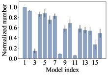
(a) Random sampling

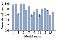
(b) Adaptive sampling

Figure 3: (a) An example of compressed models being unevenly sampled with random sampling; (b) our adaptive sampling algorithm can mitigate the unbalanced sampling problem.

IV-C Training Decision Model

Given the sampling results $\{\Psi_{1}^{sub},\Psi_{2}^{sub},\cdots,\Psi_{n}^{sub}\}$, we train an end-to-end decision model $\mathcal{M}_{decision}$ to effectively represent and distinguish $\{\Psi_{1}^{sub},\Psi_{2}^{sub},\cdots,\Psi_{n}^{sub}\}$ by employing a parameter-frozen scene representation network $\mathcal{M}_{scene}$ and neural-network-based classifier.

Specifically, we use $\mathcal{M}_{scene}$ as a backbone neural network to obtain scene representation, denoted as $h^{s}_{i}$, for every data sample $x_{i}\in\Psi_{i}^{sub},i\in[1,n]$. In this way, $h^{s}_{i}$ will retain the scene-related information. The model decision here can be formulated as a multi-class classification problem. The label of $x$ for decision model training is a vector, referred to as a model allocation vector $v^{x}=\{v_{i}^{x},i\in[1,n]\}$, where the $i$-th element $v_{i}^{x}$, denotes whether $x\in\Psi_{i}^{sub}$. The cross entropy loss function [20] is used for training the decision model. Note that during the training of decision model $\mathcal{M}_{decision}$, the parameter of $\mathcal{M}_{scene}$ is frozen to improve training efficiency and enhance the generalization of $\mathcal{M}_{decision}$ [21].

V Online Model Inference

V-A Model Selection Strategy

Given the set of pretrained models $\{\mathcal{M}_{1},\mathcal{M}_{2},\cdots,\mathcal{M}_{n}\}$ and decision model $\mathcal{M}_{decision}$ downloaded from a cloud server, a mobile device needs to select most suitable compressed models for online inference. Specifically, it utilizes $\mathcal{M}_{decision}$ to output the model allocation vector $v^{x}$ for a testing sample $x$, i.e., $v^{x}=\mathcal{M}_{decision}(x)$, where the $i$-th element $v_{i}$ indicates the suitability probability that model $\mathcal{M}_{i}$ is suitable for $x$. Therefore, we can rank all compressed models according to their suitability probablities for $x$ using $v^{x}$. It should be noted that for the uncertainty of scenario duration, model selection should be conducted on every testing sample, taking into account the fast-changing data distributions in the perspective of compressed models.

V-B Cache-based Model Deployment

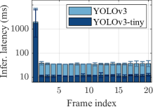
(a) Average inference latency

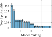
(b) Utility of compressed models

Figure 4: (a) Average latency of model inference on consecutive frames over all test clips; (b) the probability of being the top one model, following a long-tailed distribution.

With the model allocation vector $v^{x}=\mathcal{M}_{decision}(x)$, compressed models can be dynamically ranked. Due to the restricted amount of memory on a mobile device, not all models may be pre-loaded into memory. To deal with this issue, we investigate the best-effort model deployment strategy.

We examine the inference latency of detecting objects on five driving video clips, using two DNN models of different size, i.e., YOLOv3 (237MB) and YOLOv3-tiny (33.8MB), on a Nvidia Jetson TX2 NX (ARM A57 CPU, Nvidia Pascal GPU with 4GB memory, 32GB flash). Figure 4(a) plots the average inference latency of the first twenty frames over all clips. For both models, a huge delay occurs when processing the first frame. This is mainly attributed to the I/O operation for model loading and other initialization required by the deep learning framework such as Pytorch. Therefore, it is preferred to preload as many models as possible.

Given a limited video memory budget, it is tricky to pre-load best models in memory. We examine the utility of 19 YOLOv3-tiny compressed models obtained according to the algorithm stated in $\S$IV-A (see $\S$VI-A2 for more details) when conducting object detection on the five driving video clips. Figure 4(b) depicts the ratio of being the top one model over all clips for all compressed models. It can be seen that the probability of being the best model follows a power-law distribution. This observation suggests that high-level inference performance can be sustained by deploying only a small number of supreme models. Inspired by this observation, we adopt a Least Frequently Used (LFU) strategy [22] to update models in GPU memory. In the occasion of a model miss, the model with the highest suitability probability in GPU memroy will be used for inference.

VI Evaluation

VI-A Methodology

VI-A1 Datasets

We evaluate Anole on a typical mobile inference task, i.e., vehicle detection on driving videos (VD), based on the following datasets and real-world experiments.

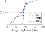
(a) CDF of image brightness

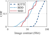
(b) CDF of image contrast

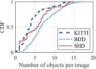
(c) CDF of the number of objects

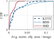
(d) CDF of the ratio of object area

Figure 5: The dataset of 64 randomly selected driving video clips demonstrates a large diversity in terms of image light conditions and foreground object distributions.

• KITTI [23]: comprises 389 stereo and optical flow image pairs, stereo visual odometry sequences of 39.2 km length, and more than 200k 3D object annotations captured in cluttered scenarios (up to 15 cars and 30 pedestrians are visible per image). For online object detection, KITTI consists of 21 training sequences and 29 test sequences.

• BDD100k [24]: contains over 100k video clips regarding ten autonomous driving tasks. Clips of 720p and 30fps were collected from more than 50 thousand rides in New York city and San Francisco Bay Area, USA. Each clip lasts for 40 seconds and is associated with semantic attributes such as the scene type (e.g., city, streets, residential areas, and highways), weather condition and the time of the day.

• SHD: contains 100 driving video clips of one minute recorded in March 2022 with a 1080p dashcam in Shanghai city, China. Clips were collected from ten typical scenarios, including highway, typical surface roads, and tunnels, at different time in the day. LabelImg [25] is employed to label objects in all images.

We random select 10 video clips from KITTI, 44 clips from BDD100k, and 10 clips from SHD, forming a dataset of 64 video clips containing 16,145 image samples in various scenarios. Figure 5 shows the cumulative distribution functions (CDFs) about foreground objects and illumination condition over all frames in the dataset, demonstrating diverse driving scenarios. We partition these 64 clips into seen (i.e., involved in model training) and unseen (i.e., not used in model training) categories with a ratio of 9:1. For each seen clip, we further divide frames into training, validation, and testing image sets with a ratio of 6:2:2.

VI-A2 Implementation

TABLE I: Anole is implemented on three different types of mobile devices with distinct hardware configurations.

Platform	CPU	GPU	GPU Memory	Flash/Disk
Jetson Nano	ARM A57	Maxwell	2GB	32GB
Jetson TX2 NX	ARM A57	Pascal	4GB	32GB
Laptop	i7-10750H	RTX 2070	8GB	1TB

We implement the offline scene profiling on a server equipped with 128GB RAM and 4 Nvidia 2080 Ti GPUs, running a Linux distribution. We implement online model inference on three typical mobile devices, i.e., a Nvidia Jetson Nano, a Nvidia Jetson TX2 NX and a Windows laptop. Pytorch is employed as the inference engine and TensorRT [26] is used for the run-time acceleration on both Jetson devices, running a Linux distribution. OpenCV is compiled on CPU for balancing the usage of CPU and GPU. The hardware configurations are shown in Table I. ResNet18 [16] and a MLP of two layers are used to train the $\mathcal{M}_{scene}$ and the $\mathcal{M}_{decision}$, respectively. Compressed models for object detection are fine-tuned on YOLOv3-tiny [17] pre-trained on the COCO [27] dataset. Details of all deployed models are listed in Table II. Compressed models are trained with Algorithm 1. A total of 19 compressed models are trained to provide compressed models for inference in all possible scenes.

TABLE II: Details of deployed models, where FLOPS of the deep model YOLOv3 is $10\times$ bigger than YOLOv3-tiny and Resnet18.

Model	Role	FLOPS	Weights
YOLOv3-tiny	Compress model	5.56 Bn	34 MB
Resnet18	$\mathcal{M}_{scene}$	4.69 Bn	44 MB
MLP	$\mathcal{M}_{decision}$	3.6 M	935 KB
YOLOv3	Deep model	65.86 Bn	237 MB

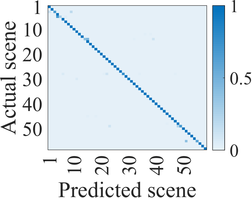
(a) $\mathcal{M}_{scene}$

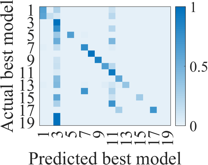
(b) $\mathcal{M}_{decision}$

Figure 6: Confusion matrices of scene profiling models, showing high accuracy for scene encoding and model decision, respectively.

VI-A3 Candidate Methods

We compare Anole with the following candidate methods:

• Single Deep Model (SDM) [17]: One single deep model is trained with all training samples for online inference, i.e., a fully-fledged YOLOv3 is trained.

• Single Shallow Model (SSM) [28]: One single compressed model is trained with all training samples for online inference, i.e., a YOLOv3-tiny is trained.

• Clustering-based Domain Generalization (CDG) [29]: Compressed models are trained on domains defined by clustering training data samples in the feature space. During online prediction, the compressed model trained on the cluster which has the closest mean compared with the feature of the test sample is selected for use.

• Dataset-based Multiple Models (DMM): One separate compressed model is trained on each training dataset, i.e., the KITTI, BDD100k, and SHD datasets. During online prediction, the compressed model corresponding to the same dataset as the test sample is selected for use.

VI-A4 Metrics

We evaluate the performance of all candidate methods with respect to inference accuracy and latency. Specifically, we use F1 score, defined as $\text{F1}=\frac{2\cdot p\cdot r}{p+r}$, where $p$ and $r$ denote the precision and recall of detection, respectively. We consider the end-to-end delay, i.e., the time duration from receiving a test sample to obtaining the corresponding inference result.

VI-B Effect of Scene Profiling Models

VI-B1 Scene Encoder $\mathcal{M}_{scene}$

We first test $\mathcal{M}_{scene}$ on classifying scenes on the validation set of seen scenes. Scenes are defined based on the multi-level clustering results. Figure 6(a) shows the scene classification confusion matrix of scene encoder $\mathcal{M}_{scene}$ on the validation set. It can be seen that $\mathcal{M}_{scene}$ works well among almost all scenes. There also exist some exceptional scenes that are confusing to $\mathcal{M}_{scene}$. We merge similar scenes in the feature space before training compressed models.

VI-B2 Decision Model $\mathcal{M}_{decision}$

We evaluate the ability of $\mathcal{M}_{decision}$ in selecting the top-one model on the validation set of seen data. Figure 6(b) show the confusion matrix of the $\mathcal{M}_{decision}$ models predicting best models versus true best models. It can be seen that $\mathcal{M}_{decision}$ have basic model selection ability. This is because the decision of model selection is based on the well-trained $\mathcal{M}_{scene}$, with one scene corresponding to a group of suitable models. We can also see that $\mathcal{M}_{decision}$ may make mistakes on some models,. This is because the top one model may not be significantly better than other models.

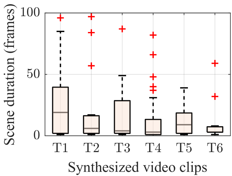
(a) Scene duration distributions on synthesized video clips

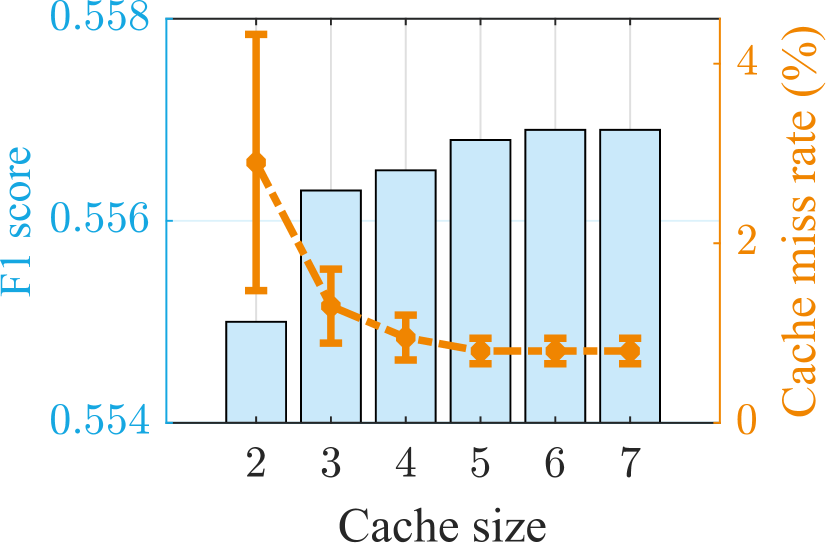
(b) Cache miss rate and F1 score obtained with varying cache size

Figure 7: (a) Boxplot of scene duration, measured as the number of frames without model switching; (b) cache miss rate and F1 score as functions of varying cache sizes.

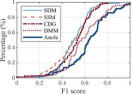
(a) KITTI

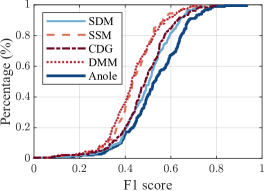
(b) BDD100k

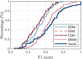
(c) SHD

Figure 8: CDFs of F1 score of all candidate methods on each source dataset, demonstrating the advantage of Anole over candidate methods, including the versatile large SDM. Note that the more the line leans towards the bottom right corner, the better the performance.

VI-C Effect of Cache-based Model Update Strategy

To effectively evaluate the effect of our cache-based model update strategy, we synthesize six fast-changing video clips, denoted as T1-T6. Specifically, for each synthesized video clip, we randomly select 5 clips from the 64 clips in the dataset. For each selected clip, we randomly cut a video segment of 100 frames (from the testing set for a seen clip) and then splice all video segments, resulting a synthesized video clip of 500 frames. We then conduct model inference using Anole on T1-T6.

VI-C1 Scene Duration

Figure 7(a) plots the boxplot of scene duration measured as the number of frames without model switching on all six synthesized video clips. It can be seen that scenes change rapidly in the perspective of $\mathcal{M}_{decision}$, with over 80% of scenes lasting fewer than 40 frames and the mean scene duration less than 20 frames.

VI-C2 Cache Miss Rate

Figure 7(b) depicts the cache miss rate and the F1 score as functions of cache size in the unit of compressed model size. It can be seen that a cache capable of loading up to 5 models can sustain a low cache miss rate and a stable inference accuracy. This observation aligns with the observation of the long-tail model utility distribution as shown in Figure 4(b). It is also observed that the inference accuracy remains satisfactory even for a cache size of 2 models, demonstrating the feasibility of Anole on devices with extremely limited GPU memory.

VI-D Cross-scene Experiments

In this experiment, we investigate the performance of all candidate methods cross fast-changing scenes, using samples in the test set of seen data. To show the instantaneous performance changes, F1 score is calculated every ten frames.

VI-D1 Performance Comparison

Figure 8 plots the CDFs of F1 score of all candidate methods on each test set of seen data selected from KITTI, BDD100k and SHD, respectively. For both tasks, Anole outwits other methods in terms of accuracy. Moreover, other methods exhibit inconsistent performance across different datasets. For example, DMM gains good performance on the KITTI and SHD datasets, while SDM only performs well on the BDD100K dataset. This discrepancy arises because DMM fits simpler datasets whereas SDM is biased towards BDD100k due to the overwhelming number of training samples.

VI-D2 Effect of Data Segmentation and Model Adaptation

It is a common practice to train an individual model on each datasets (i.e., DMM) or to segment a dataset according to feature similarity and train respective models (i.e., CDG). It can be seen that DMM performs similarly to Anole for simple training datasets such as the KITTI and the SHD datasets, but DMM performs poorly on large and complex datasets like BDD100k. In contrast, CDG trains and selects models on similar data samples. However, the inference accuracy of CDG is not as good as that of Anole over all test sets for both tasks. This demonstrates Proposition 1, which states that a model trained on a scene may not always perform well on that scene. In contrast, Anole employs a decision model to learn the appropriate scenes and determines which model is most suitable for online prediction, resulting in stable performance. Furthermore, although deep-model-based method SDM is generally assumed to have better performance, we surprisingly find that Anole outwits SDM on all test sets. This implies that training a single large DNN model for cross-scene inference is more difficult than training and choosing from a set of specialized compressed models.

VI-E New-scene Experiments

TABLE III: Inference accuracy of all candidate methods obtained on unseen data. The best results are indicated in bold while the second-best results are marked in blue.

[]

Method	KITTI	BDD100k				SHD	Mean
	St., Da.	Ur., Ni.	Ur., Da.	Hi., Du.	St., Ni.	Tu., Ni.
SDM1	0.437	0.531	0.477	0.476	0.468	0.409	0.466
SSM	0.387	0.514	0.335	0.404	0.454	0.370	0.411
CDG	0.459	0.537	0.453	0.410	0.440	0.401	0.450
DMM	0.407	0.482	0.382	0.388	0.384	0.374	0.403
Anole	0.506	0.590	0.453	0.440	0.461	0.470	0.487

• SDM uses a deep model, resulting in higher latency, larger memory usage (Table IV), and higher power consumption (Figure 11).

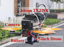
(a) Implementation of Anole on Jetson TX2 NX deployed on a UAV.

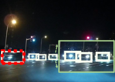
(b) Results in a typical night scenario.

Figure 9: (a) Implementation of Anole on a Jetson TX2 NX connected with a 1080p HD camera; (b) Visualization of vehicles detected in a night scenario.

In this experiment, we examine the performance of all candidate methods in new scenes, using unseen data. Particularly, six unseen video clips include one clip from KITTI with attributes of {Street, Day}, four scenes from BDD100k with attributes of {Urban, Night}, {Urban, Day}, {Highway, Dusk}, and {Street, Night}, and one scene from SHD with attributes of {Tunnel, Night}. Table III list the accuracy results. It can be seen that though SDM with a much larger model size is expected to excel other shallow-model-based methods on unseen scenes, Anole demonstrates supreme generalization ability and even outperforms SDM on all unseen data. As for unseen scenes from BDD100k, Anole can still achieve high accuracy comparable to that of SDM.

VI-F Real-world Experiments

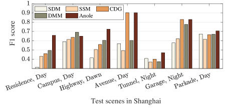
Figure 10: F1 score of all methods on test scenes in Shanghai, where Anole exceeds other methods with a latency of less than 20 ms on Jetson TX2 NX.

As depicted in Figure 9(a), we implement all methods on the Nvidia Jetson TX2 NX connected with a 1080p HD camera to conduct real-world experiments in Shanghai city. Well-trained compressed models and the decision model are downloaded to the Jetson device. We conduct real-world experiments in seven driving scenarios with different road conditions and different time in a day. LabelImg [25] is used to label all recorded frames as the ground truth for offline analysis. Figure 10 plots the F1 score of all methods. Anole outperforms all other candidate methods in all test scenarios. We visualize the car detection results of Anole (white solid frames) and SDM (red dashed frames) in a typical night driving scenario in Figure 9(b). The inference results obtained using SDM frequently contain errors, especially false negative errors as shown in the enlarged subgraph.

VI-G Inference Latency

TABLE IV: Inference latency and memory consumption on mobile devices.

	Latency (ms)			GPU Memory (MB)
	Nano	TX2 NX	Laptop	Loading model	Execution
$\mathcal{M}_{scene}$ + $\mathcal{M}_{decision}$	23.2	3.1	20.8	44	584
YOLOv3	313.8	42.9	62.2	240$\times n$1	1,730
YOLOv3-tiny	37.8	10.8	32.2	40$\times n$	1,120

• $n$ denotes the number of compressed models to load.

We evaluate the inference latency of the decision model $\mathcal{M}_{decision}$ and compressed models on different mobile devices. The results are shown in Table IV. The results reveal that YOLOv3-tiny exhibits significantly lower latency when compared to deep YOLOv3, which is generally deemed unsuitable for deployment on devices. For instance, the latency of YOLOv3-tiny on Jetson Nano is 87.9% lower than that of YOLOv3. This highlights the substantial potential for accelerating inference using shallow models. It is also evident that $\mathcal{M}_{decision}$ can be executed in real-time on embedded mobile devices such as Jetson Nano, with a latency as low as 23.2 ms, making it suitable for online inference applications.

VI-H Memory and Power Consumptions

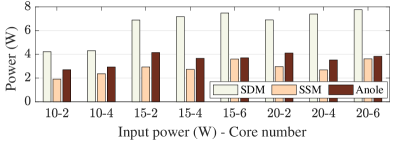
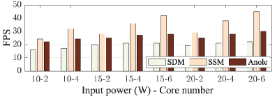
Figure 11: Power consumption and inference speed of different methods in various power modes.

We investigate the memory consumption of different models from the following two aspects, i.e., loading model only, and the memory consumption during inference with a batch size of 1. Table IV demonstrates that memory consumption for loading model is significantly lower than that during inference, owing to the presence of hidden parameters during inference. We also examine the impact of different power configurations adopted by Jetson TX2 NX to the performance of Anole. The power consumption and inference speed of Anole and baselines under different power modes are shown in Figure 11, respectively. Anole achieves a 45.1% reduction in power consumption compared with SDM and a inference speed of over 30 FPS with an input power of 20W running 6 cores.

VII Related Work

VII-A DNN Prediction on Mobile Devices

To perform DNN inference on mobile devices, new DNNs are specially designed [5, 6, 7, 8] or existing DNNs are compressed to match the computing capability of a mobile device [9, 10]. First, model structure can be optimized to reduce complexity [30, 5, 6]. Second, quantization precision can be reduced to minimize computational cost, e.g., use integers instead of floating-point numbers [31, 32]. Third, the neural network model can also be accelerated by pruning, i.e., deleting some neurons in the neural network [9, 10, 33]. Scene information is also utilized for model compression on edge/mobile devices [34, 35, 36, 37]. Finally, model distillation can distill the knowledge of large models into small models [7, 8]. Such schemes ensure real-time model inference at the expense of compromised accuracy.

Another direction is to divide DNNs and perform collaborative inference on both edge devices and the cloud [11, 12, 38, 39, 40, 41], or to transmit compressed sensory data to the cloud for data recovery and model inference [14, 15]. Neurosurgeon [12] partitions the computation of each DNN inference task in a layer granularity. CLIO [42] addresses the instability of network conditions and optimizes inference under different network states. These approaches need coordination with the cloud for each inference, leading to unpredictable inference delays when the communication link is unstable or disconnected. However, they prove inadequate for cross-scene mobile inference scenarios where even deep models are unable to cope.

VII-B Cross-scene DNN Prediction

Data-driven machine learning models face challenges in maintaining robust inference performance when dealing with cross-scene inference [43]. One natural approach for scene partitioning is to partition the scene based on prior knowledge or historical samples. First, based on prior knowledge, a similarity graph is constructed to cluster similar domains together [44]. However, obtaining such prior knowledge based on domain expertise can be challenging. Second, the original data or their extracted features can be utilized for more automated scene partitioning [45]. However, these methods may result in the loss of critical information in complex systems [29]. Cross-scene DNN prediction can also be enhanced given a golden model in the cloud for online sample labelling [46, 47]. However, the existence of a perfect or golden model is not always feasible.

VII-C Mixture of Experts

In recent years, we have witnessed the success of Mixture of Experts (MoE) [48, 49], especially in efficient training of large language models (LLM). MoE employs multiple experts for model training, each for one domain. Then, a gate network will be used to determine the correspondence between samples and experts. Though inspired by MoE, Anole differs from MoE in the following 2 aspects. First, experts in MoE are diversified by constraints of losses, but they themselves cannot be related to the scene. In fact, the main purpose of MoE is to expand the number of model parameters, rather than to customize and select scene-specific models. Second, MoE is just a model architecture, and models based on MoE architecture still need to deploy the entire model during deployment. Therefore, MoE-based models often require a significant amount of memory, which is unacceptable for mobile agents like UAVs. In contrast, Anole employs multiple compressed models for online model inference, each designed for one scene. Only a few compressed models are needed to be deployed during online inference. Therefore, Anole is more suitable for mobile devices only with limited resources.

VIII Conclusion

In this paper, we have proposed Anole, an online model inference scheme on mobile devices. Anole employs a rich set of compressed models trained on a wide variety of human-defined scenes and offline learns the implicit mode-defined scenes characterized by these compressed models via a decision model. Moreover, the most suitable compressed models can be dynamically identified according to the current testing samples and used for online model inference. As a result, Anole can deal with unseen samples, mitigating the impact of OOD problem to the reliable inference of statistical models. Anole is lightweight and does not need network connection during online inference. It can be easily implemented on various mobile devices at a low cost. Extensive experiment results demonstrate that Anole can achieve the best inference accuracy at a low latency.

References

- [1] K. Wang, X. Fu, Y. Huang, C. Cao, G. Shi, and Z.-J. Zha, “Generalized uav object detection via frequency domain disentanglement,” in Proceedings of the IEEE/CVF Conference on Computer Vision and Pattern Recognition, 2023, pp. 1064–1073.
- [2] Y. Zhou, Y. He, H. Zhu, C. Wang, H. Li, and Q. Jiang, “Monoef: Extrinsic parameter free monocular 3d object detection,” IEEE Transactions on Pattern Analysis and Machine Intelligence, vol. 44, no. 12, pp. 10 114–10 128, 2021.
- [3] Z. Zheng, J. Pu, L. Liu, D. Wang, X. Mei, S. Zhang, and Q. Dai, “Contextual anomaly detection in solder paste inspection with multi-task learning,” ACM Transactions on Intelligent Systems and Technology, vol. 11, no. 6, pp. 1–17, 2020.
- [4] Q. Chen, Z. Zheng, C. Hu, D. Wang, and F. Liu, “On-edge multi-task transfer learning: Model and practice with data-driven task allocation,” IEEE Transactions on Parallel and Distributed Systems, vol. 31, no. 6, pp. 1357–1371, 2019.
- [5] A. G. Howard, M. Zhu, B. Chen, D. Kalenichenko, W. Wang, T. Weyand, M. Andreetto, and H. Adam, “Mobilenets: Efficient convolutional neural networks for mobile vision applications,” arXiv preprint arXiv:1704.04861, 2017.
- [6] X. Zhang, X. Zhou, M. Lin, and J. Sun, “Shufflenet: An extremely efficient convolutional neural network for mobile devices,” in Proceedings of IEEE/CVF CVPR, 2018.
- [7] V. Sanh, L. Debut, J. Chaumond, and T. Wolf, “Distilbert, a distilled version of bert: smaller, faster, cheaper and lighter,” arXiv preprint arXiv:1910.01108, 2019.
- [8] X. Jiao, Y. Yin, L. Shang, X. Jiang, X. Chen, L. Li, F. Wang, and Q. Liu, “Tinybert: Distilling bert for natural language understanding,” arXiv preprint arXiv:1909.10351, 2019.
- [9] S. Han, J. Pool, J. Tran, and W. J. Dally, “Learning both weights and connections for efficient neural networks,” arXiv preprint arXiv:1506.02626, 2015.
- [10] Y. Wang, X. Zhang, L. Xie, J. Zhou, H. Su, B. Zhang, and X. Hu, “Pruning from scratch,” in Proceedings of AAAI, vol. 34, no. 07, 2020, pp. 12 273–12 280.
- [11] C. Hu, W. Bao, D. Wang, and F. Liu, “Dynamic adaptive dnn surgery for inference acceleration on the edge,” in Proceedings of IEEE INFOCOM, 2019.
- [12] Y. Kang, J. Hauswald, C. Gao, A. Rovinski, T. Mudge, J. Mars, and L. Tang, “Neurosurgeon: Collaborative intelligence between the cloud and mobile edge,” ACM SIGARCH Computer Architecture News, vol. 45, no. 1, pp. 615–629, 2017.
- [13] Y. Fang et al., “Teamnet: A collaborative inference framework on the edge,” in Proceedings of IEEE ICDCS, 2019, pp. 1487–1496.
- [14] L. Liu, H. Li, and M. Gruteser, “Edge assisted real-time object detection for mobile augmented reality,” in Proceedings of ACM MobiCom, 2019.
- [15] W. Zhang, Z. He, L. Liu, Z. Jia, and et al., “Elf: accelerate high-resolution mobile deep vision with content-aware parallel offloading,” in Proceedings of ACM MobiCom, 2021.
- [16] K. He, X. Zhang, S. Ren, and J. Sun, “Deep residual learning for image recognition,” in Proceedings of IEEE/CVF CVPR, 2016.
- [17] P. Adarsh, P. Rathi, and M. Kumar, “Yolo v3-tiny: Object detection and recognition using one stage improved model,” in Proceedings of IEEE ICACCS, 2020.
- [18] S. Lloyd, “Least squares quantization in pcm,” IEEE transactions on information theory, vol. 28, no. 2, pp. 129–137, 1982.
- [19] O. Chapelle and L. Li, “An empirical evaluation of thompson sampling,” in Proceedings of NIPS. Red Hook, NY, USA: Curran Associates Inc., 2011, p. 2249–2257.
- [20] P.-T. De Boer, D. P. Kroese, S. Mannor, and R. Y. Rubinstein, “A tutorial on the cross-entropy method,” Annals of operations research, vol. 134, no. 1, pp. 19–67, 2005.
- [21] Z. Li, K. Ren, X. Jiang, B. Li, H. Zhang, and D. Li, “Domain generalization using pretrained models without fine-tuning,” arXiv preprint arXiv:2203.04600, 2022.
- [22] A. Silberschatz, P. B. Galvin, and G. Gagne, Operating System Concepts, 10th ed. John Wiley & Sons, 2018.
- [23] A. Geiger, P. Lenz, and R. Urtasun, “Are we ready for autonomous driving? the kitti vision benchmark suite,” in Proceedings of IEEE/CVF CVPR, 2012.
- [24] F. Yu, H. Chen, X. Wang, W. Xian, Y. Chen, F. Liu, V. Madhavan, and T. Darrell, “Bdd100k: A diverse driving dataset for heterogeneous multitask learning,” in Proceedings of IEEE/CVF CVPR, June 2020.
- [25] D. Tzutalin, “Labelimg,” GitHub repository, vol. 6, 2015.
- [26] H. Vanholder, “Efficient inference with tensorrt,” in GPU Technology Conference, vol. 1, 2016, p. 2.
- [27] T.-Y. Lin, M. Maire, S. Belongie, J. Hays, P. Perona, D. Ramanan, P. Dollár, and C. L. Zitnick, “Microsoft coco: Common objects in context,” in Proceedings of ECCV, 2014.
- [28] J. Redmon and A. Farhadi, “Yolov3: An incremental improvement,” arXiv preprint arXiv:1804.02767, 2018.
- [29] Z. Zheng, Y. Wang, Q. Dai, H. Zheng, and D. Wang, “Metadata-driven task relation discovery for multi-task learning.” in Proceedings of IJCAI, 2019.
- [30] H. Chen, Y. Wang, C. Xu, B. Shi, C. Xu, Q. Tian, and C. Xu, “Addernet: Do we really need multiplications in deep learning?” in Proceedings of IEEE/CVF CVPR, 2020, pp. 1468–1477.
- [31] X. Jiang, H. Wang, Y. Chen, Z. Wu, L. Wang, B. Zou, Y. Yang, Z. Cui, Y. Cai, T. Yu, C. Lv, and Z. Wu, “Mnn: A universal and efficient inference engine,” in Proceedings of MLSys, 2020.
- [32] E. Elsen, M. Dukhan, T. Gale, and K. Simonyan, “Fast sparse convnets,” in Proceedings of IEEE/CVF CVPR, 2020, pp. 14 629–14 638.
- [33] Z. Liu, M. Sun, and Z. et al, “Rethinking the value of network pruning,” in Proceedings of ICLR, 2019.
- [34] B. Feng, Y. Wang, G. Li, Y. Xie, and Y. Ding, “Palleon: A runtime system for efficient video processing toward dynamic class skew,” in Proceedings of USENIX ATC, 2021.
- [35] R. Xu, J. Lee, P. Wang, S. Bagchi, Y. Li, and S. Chaterji, “Litereconfig: cost and content aware reconfiguration of video object detection systems for mobile gpus,” in Proceedings of EurSys, 2022.
- [36] Y. Wang, W. Wang, D. Liu, X. Jin, J. Jiang, and K. Chen, “Enabling edge-cloud video analytics for robotics applications,” IEEE Transactions on Cloud Computing, 2022.
- [37] S. Jiang, Z. Lin, Y. Li, Y. Shu, and Y. Liu, “Flexible high-resolution object detection on edge devices with tunable latency,” in Proceedings of ACM MobiCom, 2021.
- [38] A. Banitalebi-Dehkordi, N. Vedula, J. Pei, F. Xia, L. Wang, and Y. Zhang, “Auto-split: a general framework of collaborative edge-cloud ai,” in Proceedings of ACM SIGKDD, 2021.
- [39] Z. Zheng, Y. Li, H. Song, L. Wang, and F. Xia, “Towards edge-cloud collaborative machine learning: A quality-aware task partition framework,” in Proceedings of ACM CIKM, 2022.
- [40] S. Laskaridis, S. I. Venieris, M. Almeida, I. Leontiadis, and N. D. Lane, “Spinn: synergistic progressive inference of neural networks over device and cloud,” in Proceedings of ACM MobiCom, 2020.
- [41] P. Guo, B. Hu, and W. Hu, “Mistify: Automating dnn model porting for on-device inference at the edge,” in Proceedings of USENIX NSDI, 2021.
- [42] J. Huang, C. Samplawski, D. Ganesan, B. Marlin, and H. Kwon, “Clio: Enabling automatic compilation of deep learning pipelines across iot and cloud,” in Proceedings of ACM MobiCom, 2020.
- [43] S. Zhai, Z. Tang, P. Nurmi, and et al., “Rise: Robust wireless sensing using probabilistic and statistical assessments,” in Proceedings of ACM MobiCom, 2021.
- [44] L. Han, Y. Zhang, G. Song, and K. Xie, “Encoding tree sparsity in multi-task learning: A probabilistic framework,” in Proceedings of AAAI, 2014.
- [45] W. Lu, J. Wang, X. Sun, and et al., “Out-of-distribution representation learning for time series classification,” in Proceedings of ICLR, 2023.
- [46] M. Khani, G. Ananthanarayanan, K. Hsieh, J. Jiang, R. Netravali, Y. Shu, M. Alizadeh, and V. Bahl, “Recl: Responsive resource-efficient continuous learning for video analytics,” in Proceedings of USENIX NSDI, 2023.
- [47] R. Bhardwaj, Z. Xia, G. Ananthanarayanan, and et al., “Ekya: Continuous learning of video analytics models on edge compute servers,” in Proceedings of USENIX NSDI, 2022.
- [48] R. A. Jacobs, M. I. Jordan, S. J. Nowlan, and G. E. Hinton, “Adaptive mixtures of local experts,” Neural computation, vol. 3, no. 1, pp. 79–87, 1991.
- [49] N. Shazeer, A. Mirhoseini, K. Maziarz, A. Davis, Q. Le, G. Hinton, and J. Dean, “Outrageously large neural networks: The sparsely-gated mixture-of-experts layer,” in Proceedings of ICLR, 2016.