$L^{p}$-convergence of Kantorovich-type Max-Min Neural Network Operators

Abstract.

In this work, we study the Kantorovich variant of max-min neural network operators, in which the operator kernel is defined in terms of sigmoidal functions. Our main aim is to demonstrate the $L^{p}$-convergence of these nonlinear operators for $1\leq p<\infty$, which makes it possible to obtain approximation results for functions that are not necessarily continuous. In addition, we will derive quantitative estimates for the rate of approximation in the $L^{p}$-norm. We will provide some explicit examples, studying the approximation of discontinuous functions with the max-min operator, and varying additionally the underlying sigmoidal function of the kernel. Further, we numerically compare the $L^{p}$-approximation error with the respective error of the Kantorovich variants of other popular neural network operators. As a final application, we show that the Kantorovich variant has advantages compared to the sampling variant of the max-min operator and Kantorovich variant of the max-product operator when it comes to approximate noisy functions as for instance biomedical ECG signals.

1. Introduction

Neural network operators have been widely studied in approximation theory [1, 2, 3, 4, 5, 6, 7, 14, 17, 18, 19, 20, 21, 22, 28, 29, 30]. Although originally mainly linear neural network operators have been considered [1, 3, 4, 5, 14, 17, 18, 19, 31, 41], nonlinear versions of these operators have recently begun to attract the attention of several research groups [6, 7, 16, 20, 21, 22, 23, 26].

Bede et al., changing the algebraic structure of summation and multiplication, constructed pseudo-linear operators, which are in fact nonlinear [11]. Further, pseudo-linear versions of Shepard operators were investigated, and it was shown that these operators could outperform the classical ones, both, in the rate of approximation, as well as in computational complexity [11, 12]. These results were the starting point of several further research on this topic and, as far as today, a lot of studies have been conducted on pseudo-linear operators [8, 9, 10, 32, 33, 34, 35, 36, 37, 38, 39, 40, 44].

Costarelli and Spigler in [17] studied positive linear neural network operators activated by sigmoidal functions which, for sufficiently large $n\in\mathbb{N}$, are given in the form

$$F_{n}\left(f;x\right):=\dfrac{\sum\limits_{k=\left\lceil na\right\rceil}^{\left\lfloor nb\right\rfloor}f\left(\frac{k}{n}\right)\phi_{\sigma}\left(nx-k\right)}{\sum\limits_{d=\left\lceil na\right\rceil}^{\left\lfloor nb\right\rfloor}\phi_{\sigma}\left(nx-d\right)}\text{ \ \ (}x\in\left[a,b\right]\text{)},$$ (1.1)

where $\phi_{\sigma}$ is a suitable linear combination of sigmoidal activation functions $\sigma:\mathbb{R}\rightarrow\mathbb{R}$ and $f:\left[a,b\right]\rightarrow\mathbb{R}$ is a bounded function. In the definition above, $\left\lfloor\cdot\right\rfloor$ and $\left\lceil\cdot\right\rceil$ denote the floor and the ceiling function for a given number. Subsequently, Costarelli and Vinti in [20] constructed the (nonlinear) max-product operators

$$F_{n}^{\left(M\right)}\left(f;x\right):=\dfrac{\bigvee\limits_{k=\left\lceil na\right\rceil}^{\left\lfloor nb\right\rfloor}f\left(\frac{k}{n}\right)\phi_{\sigma}\left(nx-k\right)}{\bigvee\limits_{d=\left\lceil na\right\rceil}^{\left\lfloor nb\right\rfloor}\phi_{\sigma}\left(nx-d\right)}\text{ \ \ (}x\in\left[a,b\right]\text{)},$$ (1.2)

with $\bigvee\nolimits_{k=1}^{n}a_{k}:=\max\nolimits_{k=1,\cdots,n}a_{k}$, and derived a uniform approximation theorem.

Later, in [19, 21], Costarelli and his colleagues investigated also the Kantorovich form of the operators in (1.1) and (1.2). Furthermore, in [7], the (nonlinear) max-min case of these operators was examined and it was shown that compared to the positive linear neural network operators in (1.1) the max-min approximation provides better results in some cases. It is noteworthy to mention that the max-min case, in which the product is substituted by the minimum, has not been studied very profoundly so far compared to other neural network operators. We also note that the max-min operators are neither linear, nor homogeneous.

The aim of this article is to analyze the Kantorovich form of the max-min neural network operators and to obtain a convergence theorem for $L^{p}$-spaces. This allows to consider such operators also for the approximation of discontinuous functions. While the max-min variant of Kantorovich operators has already been considered in a previous article [37], to the best of our knowledge, this is the first study of the convergence of the max-min operators in $L^{p}$ spaces. Furthermore, we also aim to obtain refined estimates for the rates of approximation of these operators. The last part of the article includes some applications to better illustrate the understanding of the topic and to see in which scenarios the max-min Kantorovich form has advantages compared to max-product Kantorovich variant and max-min sampling variant of the operator.

2. Max-min neural network operators

Let $f:\left[a,b\right]\rightarrow\left[0,1\right]$ be a given function. Then, for $x\in\left[a,b\right]$, the max-min neural network operator is defined as (see [7]):

$$F_{n}^{\left(m\right)}\left(f;x\right):=\bigvee\limits_{k=\left\lceil na\right\rceil}^{\left\lfloor nb\right\rfloor}f\left(\frac{k}{n}\right)\wedge\dfrac{\phi_{\sigma}\left(nx-k\right)}{\bigvee\limits_{d=\left\lceil na\right\rceil}^{\left\lfloor nb\right\rfloor}\phi_{\sigma}\left(nx-d\right)},$$ (2.1)

where $a\wedge b$ denotes $\min\left\{a,b\right\}$. Before introducing the Kantorovich type max-min neural network operators, we need some additional definitions and assumptions.

For a given function $\sigma:\mathbb{R}\rightarrow\mathbb{R}$, we say that $\sigma$ is a sigmoidal function if $\lim_{x\rightarrow-\infty}\sigma\left(x\right)=0$ and $\lim_{x\rightarrow\infty}\sigma\left(x\right)=1.$ For the rest of the paper, we assume that $\sigma$ is a nondecreasing sigmoidal function. We also assume that $\sigma\left(3\right)>\sigma\left(1\right)$, which is only a minor restriction that prevents some technical issues.

Beside the above definitions, the following conditions are needed.

1. $\sigma\left(x\right)-1/2$ is an odd function on the real line,

2. $\sigma\in C^{2}\left(\mathbb{R}\right)$ is concave for all $x\in\mathbb{R}_{0}^{+},$

3. $\sigma\left(x\right)=O(\left|x\right|^{-(1+\alpha)})$ as $x\rightarrow-\infty$ for some $\alpha>0.$

For the rest of this paper, we use the “$\alpha$” symbol exclusively in connection to the condition specified in $\left(\Sigma 3\right)$. The kernel $\phi_{\sigma}$ (also called “centered bell shaped function” in [27]) in the definition of the neural network operator is given by

$$\phi_{\sigma}\left(x\right):=\frac{1}{2}\left(\sigma\left(x+1\right)-\sigma\left(x-1\right)\right)\text{ \ for all }x\in\mathbb{R}\text{.}$$

We note that, by definition, the kernel $\phi_{\sigma}$ is not necessarily compactly supported.

From the definitions and assumption above, it is possible to obtain the following properties of $\phi_{\sigma}$ (see[17]).

Lemma 2.1.

1. $\phi_{\sigma}\left(x\right)\geq 0$ for all $x\in\mathbb{R}$ and $\phi_{\sigma}\left(2\right)>0$,

2. $\lim_{x\rightarrow\pm\infty}\phi_{\sigma}\left(x\right)=0$,

3. $\phi_{\sigma}$ is nondecreasing if $x<0$ and nonincreasing if $x\geq 0$ (therefore $\phi_{\sigma}\left(0\right)\geq\phi_{\sigma}\left(x\right)$ for all $x\in\mathbb{R)},$

4. $\phi_{\sigma}\left(x\right)=O(\left|x\right|^{-\left(1+\alpha\right)})$ as $x\rightarrow\pm\infty$ where $\alpha$ refers to the decay rate in $\left(\Sigma 3\right),$ i.e., there exist $M,L>0$ such that $\phi_{\sigma}\left(x\right)\leq M\left|x\right|^{-\left(1+\alpha\right)}$ if $\left|x\right|>L.$

5. $\phi_{\sigma}\left(x\right)$ is an even function.

6. For all $x\in\mathbb{R},$ $\sum\limits_{k\in\mathbb{Z}}\phi_{\sigma}\left(x-k\right)=1.$

Note that from $(3)$ and $(6)$ of Lemma 2.1, it is not hard to see that $\phi_{\sigma}\in L^{1}\left(\mathbb{R}\right)$ (see also Remark 1 in [21]). Furthermore, by the definition of $\sigma$ and $\phi_{\sigma}$, we have $\phi_{\sigma}\left(x\right)\leq 1/2$ for all $x\in\mathbb{R}$.

Remark 2.1.

We note that, as in [17, 20], the condition $\left(\Sigma 2\right)$ is only used to prove Lemma 2.1 $(3)$ above. Thus, the reader can infer that our theory is also valid for non-smooth sigmoidal functions, which satisfy the property $(3)$ in Lemma 2.1 instead of the condition $\left(\Sigma 2\right)$.

The following lemma is required for the well-definiteness of the Kantorovich type operator given in (3.1).

Lemma 2.2.

(see [20])

1. For a given $x\in\mathbb{R}$,

   $$\bigvee\limits_{k\in\mathbb{Z}}\phi_{\sigma}\left(nx-k\right)\geq\phi_{\sigma}\left(2\right)>0$$

   holds for all $n\in\mathbb{N},$

2. Let the interval $\left[a,b\right]$ be given. Then for each $x\in\left[a,b\right]$

   $$\bigvee\limits_{k=\left\lceil na\right\rceil}^{\left\lfloor nb\right\rfloor-1}\phi_{\sigma}\left(nx-k\right)\geq\phi_{\sigma}\left(2\right)>0$$

   for sufficiently large $n\in\mathbb{N}$.

If the index set has infinite elements, then “$\vee$” corresponds to the supremum.

Lemma 2.3.

(see [20]) For every $\delta>0,$ we get

$$\bigvee\limits_{\overset{k\in\mathbb{Z}}{\left|x-k\right|>n\delta}}\phi_{\sigma}\left(x-k\right)=O\left(n^{-\left(1+\alpha\right)}\right)\text{ as }n\rightarrow\infty$$

uniformly in $x\in\mathbb{R}$.

We further state some well-known properties of the $\max$ and $\min$ operations.

Lemma 2.4.

(see [10]) If $\bigvee\limits_{k\in\mathbb{Z}}a_{k}<\infty$ or $\bigvee\limits_{k\in\mathbb{Z}}b_{k}<\infty$, then there holds

$$\left|\bigvee\limits_{k\in\mathbb{Z}}a_{k}-\bigvee\limits_{k\in\mathbb{Z}}b_{k}\right|\leq\bigvee\limits_{k\in\mathbb{Z}}\left|a_{k}-b_{k}\right|.$$

Lemma 2.5.

(see [11]) For all $x,y,z\in\left[0,1\right],$ there holds

$$\left|x\wedge y-x\wedge z\right|\leq x\wedge\left|y-z\right|\text{,}$$

where $a\wedge b$ denotes the $\min\left\{a,b\right\}$.

Lemma 2.6.

(see [11]) For any $a_{k}\geq 0$ and $p\geq 0,$ we have

$$\biggl{(}\bigvee\limits_{k\in\mathbb{Z}}a_{k}\biggl{)}^{p}=\bigvee\limits_{k\in\mathbb{Z}}a_{k}^{p}$$

and

$$\biggl{(}\bigwedge\limits_{k\in\mathbb{Z}}a_{k}\biggl{)}^{p}=\bigwedge\limits_{k\in\mathbb{Z}}a_{k}^{p}.$$

3. Kantorovich type max-min neural network operators

Now, instead of $f\left(\frac{k}{n}\right)$ in (2.1), taking the average value of $f$ on $\left[\frac{k}{n},\frac{k+1}{n}\right]$, we construct the Kantorovich type max-min neural network operator as follows

$$K_{n}^{\left(m\right)}\left(f;x\right):=\bigvee\limits_{k=\left\lceil na\right\rceil}^{\left\lfloor nb\right\rfloor-1}n\int\limits_{\frac{k}{n}}^{\frac{k+1}{n}}f\left(u\right)du\wedge\dfrac{\phi_{\sigma}\left(nx-k\right)}{\bigvee\limits_{d=\left\lceil na\right\rceil}^{\left\lfloor nb\right\rfloor-1}\phi_{\sigma}\left(nx-d\right)}\text{ \ \ (}x\in\left[a,b\right]\text{)},$$ (3.1)

where $f:\left[a,b\right]\rightarrow\left[0,1\right]$ is measurable and $n\in\mathbb{N}$ is sufficiently large such that $\left\lceil na\right\rceil\leq\left\lfloor nb\right\rfloor$. Lemma 2.2 guarantees that the denominator in the operator is different from zero. Therefore,

$$K_{n}^{\left(m\right)}\left(f;x\right) \leq\bigvee\limits_{k=\left\lceil na\right\rceil}^{\left\lfloor nb\right\rfloor-1}1\wedge\dfrac{\phi_{\sigma}\left(nx-k\right)}{\bigvee\limits_{d=\left\lceil na\right\rceil}^{\left\lfloor nb\right\rfloor-1}\phi_{\sigma}\left(nx-d\right)}$$

$$=\bigvee\limits_{k=\left\lceil na\right\rceil}^{\left\lfloor nb\right\rfloor-1}\dfrac{\phi_{\sigma}\left(nx-k\right)}{\bigvee\limits_{d=\left\lceil na\right\rceil}^{\left\lfloor nb\right\rfloor-1}\phi_{\sigma}\left(nx-d\right)}$$

$$=1<\infty,$$

that is, the Kantorovich type max-min operator is well-defined. Some important properties of the max-min neural network operator are given in the following lemma.

Lemma 3.1.

Let $f,g:\left[a,b\right]\rightarrow\left[0,1\right]$ be two measurable functions.

1. If $\sigma$ is continuous function on $\mathbb{R}$, then $K_{n}^{\left(m\right)}\left(f\right)$ is continuous on $\left[a,b\right]$,

2. If $f\left(x\right)\leq g\left(x\right)$ for all $x\in\left[a,b\right],$ then $K_{n}^{\left(m\right)}\left(f;x\right)\leq K_{n}^{\left(m\right)}\left(g;x\right)$ for all $x\in\left[a,b\right]$,

3. $K_{n}^{\left(m\right)}$ is sublinear, that is, $K_{n}^{\left(m\right)}\left(f+g;x\right)\leq K_{n}^{\left(m\right)}\left(f;x\right)+K_{n}^{\left(m\right)}\left(g;x\right)$ for all $x\in\left[a,b\right]$,

4. $\left|K_{n}^{\left(m\right)}\left(f;x\right)-K_{n}^{\left(m\right)}\left(g;x\right)\right|\leq K_{n}^{\left(m\right)}\left(\left|f-g\right|;x\right)$ for all $x\in\left[a,b\right]$.

The proof can be easily obtained from the definition of the operator and the lemmas above.

Remark 3.1.

Kantorovich type max-min neural network operators are not pseudo-linear in the max-min sense. Notice also that $K_{n}^{\left(m\right)}$ is not homogeneous, which means $K_{n}^{\left(m\right)}\left(cf\right)\neq cK_{n}^{\left(m\right)}\left(f\right)$ for some measurable functions $f$ and constants $c>0.$

For a fixed $\delta>0,$ $x\in\left[a,b\right]$ and $n\in\mathbb{N}$, we define $B_{\delta,n}\left(x\right)$ such that

$$B_{\delta,n}\left(x\right):=\left\{k=\left\lceil na\right\rceil,\left\lceil na\right\rceil+1,\ldots,\left\lfloor nb\right\rfloor-1:\left|x-\frac{k}{n}\right|>\delta\right\}\text{.}$$

Our approximation theorems now read as follows.

Theorem 3.2.

Let $f:\left[a,b\right]\rightarrow\left[0,1\right]$ be a measurable function. Then we have

$$\lim_{n\rightarrow\infty}K_{n}^{\left(m\right)}\left(f;x\right)=f\left(x\right)$$

at any continuity point $x\in\left[a,b\right]$ of $f.$ Furthermore, if $f\in C\left(\left[a,b\right],\left[0,1\right]\right),$ we get

$$\lim_{n\rightarrow\infty}\left\|K_{n}^{\left(m\right)}\left(f\right)-f\right\|_{\infty}=0.$$

Proof.

Let $x\in\left[a,b\right]$ be a continuity point of $f$. Adding and subtracting some suitable terms, by the triangle inequality we get

$$\left|K_{n}^{\left(m\right)}\left(f;x\right)-f\left(x\right)\right|$$

$$\leq\bigg{|}\bigvee\limits_{k=\left\lceil na\right\rceil}^{\left\lfloor nb\right\rfloor-1}n\int\limits_{\frac{k}{n}}^{\frac{k+1}{n}}f\left(u\right)du\wedge\dfrac{\phi_{\sigma}\left(nx-k\right)}{\bigvee\limits_{d=\left\lceil na\right\rceil}^{\left\lfloor nb\right\rfloor-1}\phi_{\sigma}\left(nx-d\right)}$$

$$-\bigvee\limits_{k=\left\lceil na\right\rceil}^{\left\lfloor nb\right\rfloor-1}n\int\limits_{\frac{k}{n}}^{\frac{k+1}{n}}f\left(x\right)du\wedge\dfrac{\phi_{\sigma}\left(nx-k\right)}{\bigvee\limits_{d=\left\lceil na\right\rceil}^{\left\lfloor nb\right\rfloor-1}\phi_{\sigma}\left(nx-d\right)}\bigg{|}$$

$$+\bigg{|}\bigvee\limits_{k=\left\lceil na\right\rceil}^{\left\lfloor nb\right\rfloor-1}n\int\limits_{\frac{k}{n}}^{\frac{k+1}{n}}f\left(x\right)du\wedge\dfrac{\phi_{\sigma}\left(nx-k\right)}{\bigvee\limits_{d=\left\lceil na\right\rceil}^{\left\lfloor nb\right\rfloor-1}\phi_{\sigma}\left(nx-d\right)}-f\left(x\right)\bigg{|}$$

where

$$\bigg{|}\bigvee\limits_{k=\left\lceil na\right\rceil}^{\left\lfloor nb\right\rfloor-1}n\int\limits_{\frac{k}{n}}^{\frac{k+1}{n}}f\left(x\right)du\wedge\dfrac{\phi_{\sigma}\left(nx-k\right)}{\bigvee\limits_{d=\left\lceil na\right\rceil}^{\left\lfloor nb\right\rfloor-1}\phi_{\sigma}\left(nx-d\right)}-f\left(x\right)\bigg{|}$$

$$=\bigg{|}\bigvee\limits_{k=\left\lceil na\right\rceil}^{\left\lfloor nb\right\rfloor-1}f\left(x\right)\wedge\dfrac{\phi_{\sigma}\left(nx-k\right)}{\bigvee\limits_{d=\left\lceil na\right\rceil}^{\left\lfloor nb\right\rfloor-1}\phi_{\sigma}\left(nx-d\right)}-f\left(x\right)\bigg{|}$$

$$=\bigg{|}f\left(x\right)\wedge\bigvee\limits_{k=\left\lceil na\right\rceil}^{\left\lfloor nb\right\rfloor-1}\dfrac{\phi_{\sigma}\left(nx-k\right)}{\bigvee\limits_{d=\left\lceil na\right\rceil}^{\left\lfloor nb\right\rfloor-1}\phi_{\sigma}\left(nx-d\right)}-f\left(x\right)\bigg{|}$$

$$=0.$$

Then from Lemma 2.4 and Lemma 2.5, we obtain

$$\left|K_{n}^{\left(m\right)}\left(f;x\right)-f\left(x\right)\right|$$

$$\leq\bigvee\limits_{k=\left\lceil na\right\rceil}^{\left\lfloor nb\right\rfloor-1}\bigg{|}n\int\limits_{\frac{k}{n}}^{\frac{k+1}{n}}f\left(u\right)du\wedge\dfrac{\phi_{\sigma}\left(nx-k\right)}{\bigvee\limits_{d=\left\lceil na\right\rceil}^{\left\lfloor nb\right\rfloor-1}\phi_{\sigma}\left(nx-d\right)}-n\int\limits_{\frac{k}{n}}^{\frac{k+1}{n}}f\left(x\right)du\wedge\dfrac{\phi_{\sigma}\left(nx-k\right)}{\bigvee\limits_{d=\left\lceil na\right\rceil}^{\left\lfloor nb\right\rfloor-1}\phi_{\sigma}\left(nx-d\right)}\bigg{|}$$

$$\leq\bigvee\limits_{k=\left\lceil na\right\rceil}^{\left\lfloor nb\right\rfloor-1}n\int\limits_{\frac{k}{n}}^{\frac{k+1}{n}}\left|f\left(u\right)-f\left(x\right)\right|du\wedge\dfrac{\phi_{\sigma}\left(nx-k\right)}{\bigvee\limits_{d=\left\lceil na\right\rceil}^{\left\lfloor nb\right\rfloor-1}\phi_{\sigma}\left(nx-d\right)}.$$ (3.2)

Since $f$ is continuous at the point $x,$ then for all $\varepsilon>0,$ there exists a $\delta=\delta\left(x,\varepsilon\right)>0$ such that

$$\left|f\left(y\right)-f\left(x\right)\right|<\varepsilon$$

whenever $y\in\left[x-\delta,x+\delta\right].$ Partitioning the maximum operation as follows

$$\left|K_{n}^{\left(m\right)}\left(f;x\right)-f\left(x\right)\right| \leq\bigvee\limits_{k\in B_{\frac{\delta}{2},n}\left(x\right)}n\int\limits_{\frac{k}{n}}^{\frac{k+1}{n}}\left|f\left(u\right)-f\left(x\right)\right|du\wedge\dfrac{\phi_{\sigma}\left(nx-k\right)}{\bigvee\limits_{d=\left\lceil na\right\rceil}^{\left\lfloor nb\right\rfloor-1}\phi_{\sigma}\left(nx-d\right)}$$

$$\bigvee\bigvee\limits_{k\notin B_{\frac{\delta}{2},n}\left(x\right)}n\int\limits_{\frac{k}{n}}^{\frac{k+1}{n}}\left|f\left(u\right)-f\left(x\right)\right|du\wedge\dfrac{\phi_{\sigma}\left(nx-k\right)}{\bigvee\limits_{d=\left\lceil na\right\rceil}^{\left\lfloor nb\right\rfloor-1}\phi_{\sigma}\left(nx-d\right)}$$

$$=:U_{1}\bigvee U_{2}\text{,}$$

(using the fact that $\left|u-x\right|\leq\left|u-\frac{k}{n}\right|+\left|\frac{k}{n}-x\right|\leq\frac{1}{n}+\frac{\delta}{2}\leq\delta$ for sufficiently large $n\in\mathbb{N}$ in $U_{2}$) we obtain

$$U_{2} <\bigvee\limits_{k\notin B_{\frac{\delta}{2},n}\left(x\right)}\varepsilon\wedge\dfrac{\phi_{\sigma}\left(nx-k\right)}{\bigvee\limits_{d=\left\lceil na\right\rceil}^{\left\lfloor nb\right\rfloor-1}\phi_{\sigma}\left(nx-d\right)}$$

$$\leq\varepsilon.$$

On the other hand, since $\left|f\right|\leq 1,$ from Lemma 2.3 we get

$$U_{1} \leq\bigvee\limits_{k\in B_{\frac{\delta}{2},n}\left(x\right)}1\wedge\dfrac{\phi_{\sigma}\left(nx-k\right)}{\bigvee\limits_{d=\left\lceil na\right\rceil}^{\left\lfloor nb\right\rfloor-1}\phi_{\sigma}\left(nx-d\right)}$$

$$\leq\bigvee\limits_{\left|nx-k\right|>n\frac{\delta}{2}}\dfrac{\phi_{\sigma}\left(nx-k\right)}{\phi_{\sigma}\left(2\right)}$$

$$\leq\frac{K}{\phi_{\sigma}\left(2\right)}\frac{1}{n^{1+\alpha}}$$

$$<\varepsilon.$$

for sufficiently large $n\in\mathbb{N}$, which gives the desired result.

For the second part of the theorem, if $f\in C\left(\left[a,b\right],\left[0,1\right]\right)$, then using a similar argumentation lines, and noting that $\delta=\delta\left(\varepsilon\right)\,$, one can easily complete the proof. ∎

Theorem 3.3.

Let $f\in C\left(\left[a,b\right],\left[0,1\right]\right).$ Then

$$\lim_{n\rightarrow\infty}\left\|K_{n}^{\left(m\right)}\left(f\right)-f\right\|_{p}=0,$$

where $\left\|\cdot\right\|_{p}$ denotes the $L^{p}$ norm on $\left[a,b\right]\$ for $1\leq p<\infty$.

Proof.

Since from the previous theorem

$$\left\|K_{n}^{\left(m\right)}\left(f\right)-f\right\|_{\infty}<\varepsilon$$

for sufficiently large $n\in\mathbb{N}$, then we get

$$\left\|K_{n}^{\left(m\right)}\left(f\right)-f\right\|_{p} =\biggl{(}\int\limits_{a}^{b}\left|K_{n}^{\left(m\right)}\left(f;x\right)-f\left(x\right)\right|^{p}dx\biggl{)}^{\frac{1}{p}}$$

$$\leq\left\|K_{n}^{\left(m\right)}\left(f\right)-f\right\|_{\infty}\left(b-a\right)^{1/p}$$

$$<\varepsilon\left(b-a\right)^{\frac{1}{p}}$$

for sufficiently large $n\in\mathbb{N}$, which completes the proof. ∎

Theorem 3.4.

Let $f\in L^{p}\left(\left[a,b\right],\left[0,1\right]\right)$ for $1\leq p<\infty$. Then we have

$$\lim_{n\rightarrow\infty}\left\|K_{n}^{\left(m\right)}\left(f\right)-f\right\|_{p}=0\text{.}$$

Proof.

Let $f\in L^{p}\left(\left[a,b\right],\left[0,1\right]\right)$ for $1\leq p<\infty.$ Since $C\left(\left[a,b\right],\left[0,1\right]\right)$ is dense in $L^{p}\left(\left[a,b\right],\left[0,1\right]\right),$ then for all $\varepsilon>0,$ there exists a $g\in C\left(\left[a,b\right],\left[0,1\right]\right)$ such that

$$\left\|f-g\right\|_{p}<\varepsilon.$$

Now, we know that

$$\left\|K_{n}^{\left(m\right)}\left(f\right)-f\right\|_{p} \leq\left\|K_{n}^{\left(m\right)}\left(f\right)-K_{n}^{\left(m\right)}\left(g\right)\right\|_{p}+\left\|K_{n}^{\left(m\right)}\left(g\right)-g\right\|_{p}+\left\|g-f\right\|_{p}$$ (3.3)

$$<\left\|K_{n}^{\left(m\right)}\left(f\right)-K_{n}^{\left(m\right)}\left(g\right)\right\|_{p}+\left\|K_{n}^{\left(m\right)}\left(g\right)-g\right\|_{p}+\varepsilon.$$

By Theorem 3.3, we have

$$\left\|K_{n}^{\left(m\right)}\left(g\right)-g\right\|_{p}<\varepsilon$$

for sufficiently large $n\in\mathbb{N}.$ On the other hand, from Lemma 3.1 (d), we know that

$$\left\|K_{n}^{\left(m\right)}\left(f\right)-K_{n}^{\left(m\right)}\left(g\right)\right\|_{p}$$

$$=\biggl{(}\int\limits_{a}^{b}\left|K_{n}^{\left(m\right)}\left(f;x\right)-K_{n}^{\left(m\right)}\left(g;x\right)\right|^{p}dx\biggl{)}^{\frac{1}{p}}$$

$$\leq\biggl{(}\int\limits_{a}^{b}\biggl{[}\bigvee\limits_{k=\left\lceil na\right\rceil}^{\left\lfloor nb\right\rfloor-1}n\int\limits_{\frac{k}{n}}^{\frac{k+1}{n}}\left|f\left(u\right)-g\left(u\right)\right|du\wedge\dfrac{\phi_{\sigma}\left(nx-k\right)}{\bigvee\limits_{d=\left\lceil na\right\rceil}^{\left\lfloor nb\right\rfloor-1}\phi_{\sigma}\left(nx-d\right)}\biggr{]}^{p}dx\biggl{)}^{\frac{1}{p}}$$

holds true. Further, from Lemma 2.6, we obtain

$$\left\|K_{n}^{\left(m\right)}\left(f\right)-K_{n}^{\left(m\right)}\left(g\right)\right\|_{p}$$

$$\leq\biggl{(}\int\limits_{a}^{b}\bigvee\limits_{k=\left\lceil na\right\rceil}^{\left\lfloor nb\right\rfloor-1}\biggl{(}n\int\limits_{\frac{k}{n}}^{\frac{k+1}{n}}\left|f\left(u\right)-g\left(u\right)\right|du\biggl{)}^{p}\wedge\biggl{(}\dfrac{\phi_{\sigma}\left(nx-k\right)}{\bigvee\limits_{d=\left\lceil na\right\rceil}^{\left\lfloor nb\right\rfloor-1}\phi_{\sigma}\left(nx-d\right)}\biggl{)}^{p}dx\biggl{)}^{\frac{1}{p}}.$$

Now, considering

$$\dfrac{\phi_{\sigma}\left(nx-k\right)}{\bigvee\limits_{d=\left\lceil na\right\rceil}^{\left\lfloor nb\right\rfloor-1}\phi_{\sigma}\left(nx-d\right)}\leq 1\text{,}$$

then by the convexity of $\left|\cdot\right|^{p}$ and Jensen’s inequality, we have

$$\left\|K_{n}^{\left(m\right)}\left(f\right)-K_{n}^{\left(m\right)}\left(g\right)\right\|_{p}$$

$$\leq\biggl{(}\int\limits_{a}^{b}\bigvee\limits_{k=\left\lceil na\right\rceil}^{\left\lfloor nb\right\rfloor-1}n\int\limits_{\frac{k}{n}}^{\frac{k+1}{n}}\left|f\left(u\right)-g\left(u\right)\right|^{p}du\wedge\dfrac{\phi_{\sigma}\left(nx-k\right)}{\bigvee\limits_{d=\left\lceil na\right\rceil}^{\left\lfloor nb\right\rfloor-1}\phi_{\sigma}\left(nx-d\right)}dx\biggl{)}^{\frac{1}{p}}$$

$$=\biggl{(}\int\limits_{a}^{b}n\bigvee\limits_{k=\left\lceil na\right\rceil}^{\left\lfloor nb\right\rfloor-1}\int\limits_{\frac{k}{n}}^{\frac{k+1}{n}}\left|f\left(u\right)-g\left(u\right)\right|^{p}du\wedge\dfrac{\phi_{\sigma}\left(nx-k\right)}{n\bigvee\limits_{d=\left\lceil na\right\rceil}^{\left\lfloor nb\right\rfloor-1}\phi_{\sigma}\left(nx-d\right)}dx\biggl{)}^{\frac{1}{p}}$$

$$\leq\biggl{(}\int\limits_{a}^{b}n\bigvee\limits_{k=\left\lceil na\right\rceil}^{\left\lfloor nb\right\rfloor-1}\int\limits_{\frac{k}{n}}^{\frac{k+1}{n}}\left|f\left(u\right)-g\left(u\right)\right|^{p}du\wedge\dfrac{\phi_{\sigma}\left(nx-k\right)}{\bigvee\limits_{d=\left\lceil na\right\rceil}^{\left\lfloor nb\right\rfloor-1}\phi_{\sigma}\left(nx-d\right)}dx\biggl{)}^{\frac{1}{p}}$$

$$\leq\biggl{(}\int\limits_{\mathbb{R}}n\bigvee\limits_{k=\left\lceil na\right\rceil}^{\left\lfloor nb\right\rfloor-1}\int\limits_{\frac{k}{n}}^{\frac{k+1}{n}}\left|f\left(u\right)-g\left(u\right)\right|^{p}du\wedge\dfrac{\phi_{\sigma}\left(nx-k\right)}{\phi_{\sigma}\left(2\right)}dx\biggl{)}^{\frac{1}{p}}.$$

After substituting $nx-k=y$, we see that

$$\left\|K_{n}^{\left(m\right)}\left(f\right)-K_{n}^{\left(m\right)}\left(g\right)\right\|_{p} \leq\biggl{(}\int\limits_{\mathbb{R}}\biggl{\{}\bigvee\limits_{k=\left\lceil na\right\rceil}^{\left\lfloor nb\right\rfloor-1}\int\limits_{\frac{k}{n}}^{\frac{k+1}{n}}\left|f\left(u\right)-g\left(u\right)\right|^{p}du\wedge\dfrac{\phi_{\sigma}\left(y\right)}{\phi_{\sigma}\left(2\right)}\biggl{\}}dy\biggl{)}^{\frac{1}{p}}$$

$$=\biggl{(}\int\limits_{\mathbb{R}}\biggl{\{}\dfrac{\phi_{\sigma}\left(y\right)}{\phi_{\sigma}\left(2\right)}\wedge\bigvee\limits_{k=\left\lceil na\right\rceil}^{\left\lfloor nb\right\rfloor-1}\int\limits_{\frac{k}{n}}^{\frac{k+1}{n}}\left|f\left(u\right)-g\left(u\right)\right|^{p}du\biggl{\}}dy\biggl{)}^{\frac{1}{p}}$$

$$\leq\biggl{(}\int\limits_{\mathbb{R}}\biggl{\{}\dfrac{\phi_{\sigma}\left(y\right)}{\phi_{\sigma}\left(2\right)}\wedge\sum\limits_{k=\left\lceil na\right\rceil}^{\left\lfloor nb\right\rfloor-1}\int\limits_{\frac{k}{n}}^{\frac{k+1}{n}}\left|f\left(u\right)-g\left(u\right)\right|^{p}du\biggl{\}}dy\biggl{)}^{\frac{1}{p}}$$

$$\leq\biggl{(}\int\limits_{\mathbb{R}}\dfrac{\phi_{\sigma}\left(y\right)}{\phi_{\sigma}\left(2\right)}\wedge\left\|f-g\right\|_{p}^{p}dy\biggl{)}^{\frac{1}{p}}.$$

Now, since $\phi_{\sigma}\in L^{1}\left(\mathbb{R}\right)$ and $\phi_{\sigma}\left(y\right)=O\left(\left|y\right|^{-\left(1+\alpha\right)}\right)$ for some $\alpha>0$, there exists $M,N>0$ (which are independent from each other) such that

$$\phi_{\sigma}\left(y\right)\leq\frac{M}{\left|y\right|^{1+\alpha}}$$

for $\left|y\right|\geq N.$ Assume that $\left\|f-g\right\|_{p}$ is sufficiently small such that

$$\tilde{N}:=\frac{1}{\left\|f-g\right\|_{p}^{\frac{p}{1+\alpha}}}\geq N,$$

then, by the following separation of the integral, we get

$$\left\|K_{n}^{\left(m\right)}\left(f\right)-K_{n}^{\left(m\right)}\left(g\right)\right\|_{p}$$

$$\leq\biggl{(}\int\limits_{\left|y\right|>\tilde{N}}\dfrac{\phi_{\sigma}\left(y\right)}{\phi_{\sigma}\left(2\right)}\wedge\left\|f-g\right\|_{p}^{p}dy+\int\limits_{\left|y\right|\leq\tilde{N}}\dfrac{\phi_{\sigma}\left(y\right)}{\phi_{\sigma}\left(2\right)}\wedge\left\|f-g\right\|_{p}^{p}dy\biggl{)}^{\frac{1}{p}}$$

$$\leq\biggl{(}\int\limits_{\left|y\right|>\tilde{N}}\dfrac{\phi_{\sigma}\left(y\right)}{\phi_{\sigma}\left(2\right)}dy+\int\limits_{\left|y\right|\leq\tilde{N}}\left\|f-g\right\|_{p}^{p}dy\biggl{)}^{\frac{1}{p}}$$

$$\leq\left(\frac{M}{\phi_{\sigma}\left(2\right)}\int\limits_{\left|y\right|>\tilde{N}}\frac{1}{\left|y\right|^{1+\alpha}}dy+2\tilde{N}\left\|f-g\right\|_{p}^{p}\right)^{\frac{1}{p}}.$$

Since $$\phi_{\sigma}$$ is even, we can conclude that

$$\left\|K_{n}^{\left(m\right)}\left(f\right)-K_{n}^{\left(m\right)}\left(g\right)\right\|_{p} \leq\left(\frac{2M}{\phi_{\sigma}\left(2\right)}\int\limits_{\tilde{N}}^{\infty}\frac{1}{y^{1+\alpha}}dy+\frac{2}{\left\|f-g\right\|_{p}^{\frac{p}{1+\alpha}}}\left\|f-g\right\|_{p}^{p}\right)^{\frac{1}{p}}$$

$$=\left(\frac{2M}{\alpha\phi_{\sigma}\left(2\right)}\left\|f-g\right\|_{p}^{\frac{\alpha p}{1+\alpha}}+2\left\|f-g\right\|_{p}^{p-\frac{p}{1+\alpha}}\right)^{\frac{1}{p}}$$

$$=\left(\left\{\frac{2M}{\alpha\phi_{\sigma}\left(2\right)}+2\right\}\left\|f-g\right\|_{p}^{\frac{\alpha p}{1+\alpha}}\right)^{\frac{1}{p}}$$

$$=\left\{\frac{2M}{\alpha\phi_{\sigma}\left(2\right)}+2\right\}^{\frac{1}{p}}\left\|f-g\right\|_{p}^{\frac{\alpha}{1+\alpha}}$$ (3.5)

$$<\left\{\frac{2M}{\alpha\phi_{\sigma}\left(2\right)}+2\right\}^{\frac{1}{p}}\varepsilon^{\frac{\alpha}{1+\alpha}}$$

holds. Therefore, by the arbitrariness of $\varepsilon$, the proof is complete. ∎

Remark 3.2.

Although we have shown the $L^{p}$-approximation only for functions $f\in L^{p}\left(\left[a,b\right],\left[0,1\right]\right)$, it is possible to extend the results for functions $f\in L^{p}\left(\left[a,b\right],\mathbb{R}\right)$ by extending the definition of the operator $K_{n}^{\left(m\right)}$ with respect to the range of the functions in $L^{p}\left(\left[a,b\right],\mathbb{R}\right)$ (see Remark 3.1 in [7], see also [38]).

4. Estimates for the Kantorovich type max-min neural network operators

Let $f:\left[a,b\right]\rightarrow\left[0,1\right]$ be given. Then for a $\delta>0,$ the modulus of continuity of $f$ on $\left[a,b\right]$ is defined by

$$\omega_{\left[a,b\right]}\left(f,\delta\right):=\sup_{\left|x-y\right|\leq\delta}\left\{\left|f\left(x\right)-f\left(y\right)\right|:x,y\in\left[a,b\right]\right\}\text{.}$$

We also need the definition of generalized absolute moment of order $\beta>0$, introduced in [20] such that for a given $\phi_{\sigma}$, it is defined as follows,

$$m_{\beta}\left(\phi_{\sigma}\right):=\sup_{x\in\mathbb{R}}\left\{\bigvee\limits_{k\in\mathbb{Z}}\phi_{\sigma}\left(x-k\right)\left|x-k\right|^{\beta}\right\}\text{.}$$

Lemma 4.1.

(see [20]) If $0<\beta\leq 1+\alpha$, then $m_{\beta}\left(\phi_{\sigma}\right)<\infty$.

Now, we investigate the rate of approximation for Theorem 3.2.

Theorem 4.2.

Let $f\in C\left(\left[a,b\right],\left[0,1\right]\right)$ and $\delta_{n}$ be a null sequence of positive real numbers being $\left(n\delta_{n}\right)^{-1}$ a null sequence. Then, we have

$$\left\|K_{n}^{\left(m\right)}\left(f\right)-f\right\|_{\infty}=\omega_{\left[a,b\right]}\left(f,n^{-1}\right)+\omega_{\left[a,b\right]}\left(f,\delta_{n}\right){\displaystyle\bigvee}\frac{m_{\left(1+\alpha\right)}\left(\phi_{\sigma}\right)}{\phi_{\sigma}\left(2\right)}\left(n\delta_{n}\right)^{-\left(1+\alpha\right)}\text{.}$$

Proof.

From (3.2), we  know that

$$\left|K_{n}^{\left(m\right)}\left(f;x\right)-f\left(x\right)\right|\leq\bigvee\limits_{k=\left\lceil na\right\rceil}^{\left\lfloor nb\right\rfloor-1}n\int\limits_{\frac{k}{n}}^{\frac{k+1}{n}}\left|f\left(u\right)-f\left(x\right)\right|du\wedge\dfrac{\phi_{\sigma}\left(nx-k\right)}{\bigvee\limits_{d=\left\lceil na\right\rceil}^{\left\lfloor nb\right\rfloor-1}\phi_{\sigma}\left(nx-d\right)}$$

holds. Since $\left|f\left(u\right)-f\left(x\right)\right|\leq\left|f\left(u\right)-f\left(\frac{k}{n}\right)\right|+\left|f\left(\frac{k}{n}\right)-f\left(x\right)\right|$ and $\left(a+b\right)\wedge c\leq a\wedge c+b\wedge c$ for all $a,b,c\geq 0$, the following inequality holds true

$$\left|K_{n}^{\left(m\right)}\left(f;x\right)-f\left(x\right)\right| \leq\bigvee\limits_{k=\left\lceil na\right\rceil}^{\left\lfloor nb\right\rfloor-1}n\int\limits_{\frac{k}{n}}^{\frac{k+1}{n}}\left|f\left(u\right)-f\left(\frac{k}{n}\right)\right|du\wedge\dfrac{\phi_{\sigma}\left(nx-k\right)}{\bigvee\limits_{d=\left\lceil na\right\rceil}^{\left\lfloor nb\right\rfloor-1}\phi_{\sigma}\left(nx-d\right)}$$

$$+\bigvee\limits_{k=\left\lceil na\right\rceil}^{\left\lfloor nb\right\rfloor-1}n\int\limits_{\frac{k}{n}}^{\frac{k+1}{n}}\left|f\left(\frac{k}{n}\right)-f\left(x\right)\right|du\wedge\dfrac{\phi_{\sigma}\left(nx-k\right)}{\bigvee\limits_{d=\left\lceil na\right\rceil}^{\left\lfloor nb\right\rfloor-1}\phi_{\sigma}\left(nx-d\right)}$$ (4.1)

$$=:I_{1}+I_{2}\text{,}$$

where the integral in $I_{2}$ does not depend on $u$ and hence

$$I_{2}=\bigvee\limits_{k=\left\lceil na\right\rceil}^{\left\lfloor nb\right\rfloor-1}\left|f\left(\frac{k}{n}\right)-f\left(x\right)\right|\wedge\dfrac{\phi_{\sigma}\left(nx-k\right)}{\bigvee\limits_{d=\left\lceil na\right\rceil}^{\left\lfloor nb\right\rfloor-1}\phi_{\sigma}\left(nx-d\right)}.$$

If we divide $I_{2}$ as given below

$$I_{2} =\bigvee\limits_{k\in B_{\delta_{n},n}\left(x\right)}\left|f\left(\frac{k}{n}\right)-f\left(x\right)\right|\wedge\dfrac{\phi_{\sigma}\left(nx-k\right)}{\bigvee\limits_{d=\left\lceil na\right\rceil}^{\left\lfloor nb\right\rfloor-1}\phi_{\sigma}\left(nx-d\right)}$$

$$\bigvee\bigvee\limits_{k\notin B_{\delta_{n},n}\left(x\right)}\left|f\left(\frac{k}{n}\right)-f\left(x\right)\right|\wedge\dfrac{\phi_{\sigma}\left(nx-k\right)}{\bigvee\limits_{d=\left\lceil na\right\rceil}^{\left\lfloor nb\right\rfloor-1}\phi_{\sigma}\left(nx-d\right)}$$

$$=:I_{2}^{1}{\textstyle\bigvee}I_{2}^{2}$$

then

$$I_{2}^{2} \leq\bigvee\limits_{k\notin B_{\delta_{n},n}\left(x\right)}\omega_{\left[a,b\right]}\left(f,\delta_{n}\right)\wedge\dfrac{\phi_{\sigma}\left(nx-k\right)}{\bigvee\limits_{d=\left\lceil na\right\rceil}^{\left\lfloor nb\right\rfloor-1}\phi_{\sigma}\left(nx-d\right)}$$

$$\leq\omega_{\left[a,b\right]}\left(f,\delta_{n}\right)$$

holds. In $I_{2}^{1}$ since $k\in B_{\delta_{n},n}\left(x\right),$ we get $\frac{\left|nx-k\right|^{1+\alpha}}{\left(n\delta_{n}\right)^{1+\alpha}}>1$ and therefore

$$I_{2}^{1} \leq\bigvee\limits_{k\in B_{\delta_{n},n}\left(x\right)}\left|f\left(\frac{k}{n}\right)-f\left(x\right)\right|\wedge\dfrac{\phi_{\sigma}\left(nx-k\right)}{\bigvee\limits_{d=\left\lceil na\right\rceil}^{\left\lfloor nb\right\rfloor-1}\phi_{\sigma}\left(nx-d\right)}$$

$$\leq\bigvee\limits_{k\in B_{\delta_{n},n}\left(x\right)}\dfrac{\phi_{\sigma}\left(nx-k\right)}{\phi_{\sigma}\left(2\right)}$$

$$\leq\bigvee\limits_{k\in B_{\delta_{n},n}\left(x\right)}\dfrac{\phi_{\sigma}\left(nx-k\right)}{\phi_{\sigma}\left(2\right)}\frac{\left|nx-k\right|^{1+\alpha}}{\left(n\delta_{n}\right)^{1+\alpha}}$$

$$\leq\frac{m_{\left(1+\alpha\right)}\left(\phi_{\sigma}\right)}{\phi_{\sigma}\left(2\right)}\frac{1}{\left(n\delta_{n}\right)^{1+\alpha}}$$

holds, where $m_{\left(1+\alpha\right)}\left(\phi_{\sigma}\right)$ is finite from Lemma 4.1. Now using the well known properties of modulus of continutiy in $I_{1}$, we obtain

$$I_{1} \leq\bigvee\limits_{k=\left\lceil na\right\rceil}^{\left\lfloor nb\right\rfloor-1}n\int\limits_{\frac{k}{n}}^{\frac{k+1}{n}}\omega_{\left[a,b\right]}\left(f,\left|u-\frac{k}{n}\right|\right)du\wedge\dfrac{\phi_{\sigma}\left(nx-k\right)}{\bigvee\limits_{d=\left\lceil na\right\rceil}^{\left\lfloor nb\right\rfloor-1}\phi_{\sigma}\left(nx-d\right)}$$

$$\leq\bigvee\limits_{k=\left\lceil na\right\rceil}^{\left\lfloor nb\right\rfloor-1}\omega_{\left[a,b\right]}\left(f,\frac{1}{n}\right)\wedge\dfrac{\phi_{\sigma}\left(nx-k\right)}{\bigvee\limits_{d=\left\lceil na\right\rceil}^{\left\lfloor nb\right\rfloor-1}\phi_{\sigma}\left(nx-d\right)}$$

$$=\omega_{\left[a,b\right]}\left(f,\frac{1}{n}\right)\text{,}$$

which completes the proof. ∎

In the above theory, if we consider the Hölder continuous functions of order $\beta$, that is, for a given $\beta\in(0,1],$ $Lip_{\left[a,b\right]}\left(\beta\right)$ is defined by

$$Lip_{\left[a,b\right]}\left(\beta\right) :=\{f\in C\left(\left[a,b\right],\left[0,1\right]\right):\exists K>0\text{ such that }\left|f\left(x\right)-f\left(y\right)\right|\leq K\left|x-y\right|^{\beta}$$

$$\left.\text{ \ \ \ \ \ for all~{}}x,y\in\left[a,b\right]\right\}\text{,}$$

then we get the following rate of approximation.

Corollary 4.3.

Let $f\in Lip_{\left[a,b\right]}\left(\beta\right)$. Then

$$\left\|K_{n}^{\left(m\right)}\left(f\right)-f\right\|_{\infty}=O\left(n^{-\frac{\left(1+\alpha\right)\beta}{1+\alpha+\beta}}\right)\text{ as }n\rightarrow\infty$$

holds.

Proof.

Since $f\in Lip_{\left[a,b\right]}\left(\beta\right)$, from (4.1) we can easily see that

$$\left|K_{n}^{\left(m\right)}\left(f;x\right)-f\left(x\right)\right| \leq\bigvee\limits_{k=\left\lceil na\right\rceil}^{\left\lfloor nb\right\rfloor-1}Kn\int\limits_{\frac{k}{n}}^{\frac{k+1}{n}}\left(u-\frac{k}{n}\right)^{\beta}du\wedge\dfrac{\phi_{\sigma}\left(nx-k\right)}{\bigvee\limits_{d=\left\lceil na\right\rceil}^{\left\lfloor nb\right\rfloor-1}\phi_{\sigma}\left(nx-d\right)}$$

$$+\bigvee\limits_{k=\left\lceil na\right\rceil}^{\left\lfloor nb\right\rfloor-1}Kn\int\limits_{\frac{k}{n}}^{\frac{k+1}{n}}\left|\frac{k}{n}-x\right|^{\beta}du\wedge\dfrac{\phi_{\sigma}\left(nx-k\right)}{\bigvee\limits_{d=\left\lceil na\right\rceil}^{\left\lfloor nb\right\rfloor-1}\phi_{\sigma}\left(nx-d\right)}$$

$$=:J_{1}+J_{2}$$

where

$$J_{1}=\frac{K}{\left(\beta+1\right)n^{\beta}}$$

for some $K>0$. Taking $\delta_{n}=\dfrac{1}{n^{\left(1+\alpha\right)/\left(1+\alpha+\beta\right)}}$, if we seperate the maximum operation in $J_{2}$ as follows,

$$J_{2} =\bigvee\limits_{k\in B_{\delta_{n},n}\left(x\right)}Kn\int\limits_{\frac{k}{n}}^{\frac{k+1}{n}}\left|\frac{k}{n}-x\right|^{\beta}du\wedge\dfrac{\phi_{\sigma}\left(nx-k\right)}{\bigvee\limits_{d=\left\lceil na\right\rceil}^{\left\lfloor nb\right\rfloor-1}\phi_{\sigma}\left(nx-d\right)}$$

$${\displaystyle\bigvee}\bigvee\limits_{k\notin B_{\delta_{n},n}\left(x\right)}Kn\int\limits_{\frac{k}{n}}^{\frac{k+1}{n}}\left|\frac{k}{n}-x\right|^{\beta}du\wedge\dfrac{\phi_{\sigma}\left(nx-k\right)}{\bigvee\limits_{d=\left\lceil na\right\rceil}^{\left\lfloor nb\right\rfloor-1}\phi_{\sigma}\left(nx-d\right)}$$

$$=:J_{2}^{1}{\textstyle\bigvee}J_{2}^{2}$$

then there holds

$$J_{2}^{1} \leq\bigvee\limits_{k\in B_{\delta_{n},n}\left(x\right)}\dfrac{\phi_{\sigma}\left(nx-k\right)}{\bigvee\limits_{d=\left\lceil na\right\rceil}^{\left\lfloor nb\right\rfloor-1}\phi_{\sigma}\left(nx-d\right)}$$ (4.2)

$$\leq\bigvee\limits_{k\in B_{\delta_{n},n}\left(x\right)}\dfrac{\phi_{\sigma}\left(nx-k\right)}{\phi_{\sigma}\left(2\right)}\frac{\left|nx-k\right|^{1+\alpha}}{\left(n\delta_{n}\right)^{1+\alpha}}$$

$$\leq\frac{m_{1+\alpha}\left(\phi_{\sigma}\right)}{\phi_{\sigma}\left(2\right)}\frac{1}{n^{\frac{\beta\left(1+\alpha\right)}{1+\alpha+\beta}}}\text{.}$$

On the other hand, since $k\notin B_{\delta_{n},n}\left(x\right)$ in $J_{2}^{2}$ we have

$$J_{2}^{2} \leq\bigvee\limits_{k\notin B_{\delta_{n},n}\left(x\right)}K\left(\delta_{n}\right)^{\beta}\wedge\dfrac{\phi_{\sigma}\left(nx-k\right)}{\bigvee\limits_{d=\left\lceil na\right\rceil}^{\left\lfloor nb\right\rfloor-1}\phi_{\sigma}\left(nx-d\right)}$$ (4.3)

$$\leq\frac{K}{n^{\frac{\beta\left(1+\alpha\right)}{1+\alpha+\beta}}}\text{.}$$

Finally, since

$$\frac{K}{\left(\beta+1\right)n^{\beta}}\leq\frac{1}{n^{\frac{\beta\left(1+\alpha\right)}{1+\alpha+\beta}}}$$ (4.4)

for sufficiently large $n\in\mathbb{N}$, from (4.2), (4.3) and (4.4) we conclude

$$\left\|K_{n}^{\left(m\right)}\left(f\right)-f\right\|_{\infty}=O\left(n^{-\frac{\left(1+\alpha\right)\beta}{1+\alpha+\beta}}\right)\text{ as }n\rightarrow\infty\text{.}$$

∎

In this part, inspired by [15, 24, 25], we provide quantitative estimates for Kantorovich type max-min neural network operators with the help of $K$-functionals introduced by Peetre in [43]. First we recall the definition of $K$-functionals, which is adapted to max-min case. For a given $f\in L^{p}\left(\left[a,b\right],\left[0,1\right]\right)$ $(1\leq p<\infty)$

$$\mathcal{K}\left(f,\delta\right)_{p}:=\inf_{g\in C^{1}\left(\left[a,b\right],\left[0,1\right]\right)}\left\{\left\|f-g\right\|_{p}^{\frac{\alpha}{\alpha+1}}+\delta\left\|g^{\prime}\right\|_{\infty}\right\}$$

where $\delta>0$. According to this definition, $\mathcal{K}\left(f,\delta\right)_{p}<\varepsilon$ $\left(\varepsilon>0\right)$ for sufficiently small $\delta>0$ means that $f$ can be approximated with an error $\left\|f-g\right\|_{p}<\varepsilon^{\frac{\alpha+1}{\alpha}},$ where $g\in C^{1}\left(\left[a,b\right],\left[0,1\right]\right)\subset L^{p}\left(\left[a,b\right],\left[0,1\right]\right)$ and whose derivative under supremum norm is not too large. $K$-functionals provide us some information about the smoothness and approximation properties of $f$, and may be considered as a modulus of smoothness in some situations in $L^{p}$ spaces. For the importance of $K$-functionals in approximation theory, we refer to [13].

Theorem 4.4.

Let $f\in L^{p}\left(\left[a,b\right],\left[0,1\right]\right)$ for $1\leq p<\infty$. Then we have

$$\left\|K_{n}^{\left(m\right)}\left(f\right)-f\right\|_{p}\leq A\mathcal{K}\left(f,Bn^{-\frac{1+\alpha}{2+\alpha}}\right)_{p}+\frac{m_{\left(1+\alpha\right)}\left(\phi_{\sigma}\right)\left(b-a\right)^{\frac{1}{p}}}{\phi_{\sigma}\left(2\right)}n^{-\frac{1+\alpha}{2+\alpha}}$$

where $A=\left[\left\{\frac{2M}{\alpha\phi_{\sigma}\left(2\right)}+2\right\}^{\frac{1}{p}}+\left(b-a\right)^{\frac{1}{p\left(1+\alpha\right)}}\right]$ and $B=\frac{\left(3/2\right)\left(b-a\right)^{\frac{1}{p}}}{A}$.

Proof.

Let $g\in C^{1}\left(\left[a,b\right],\left[0,1\right]\right)$ be given. We know from (3.3) and (3.5) that

$$\left\|K_{n}^{\left(m\right)}\left(f\right)-f\right\|_{p}$$

$$\leq\left\|K_{n}^{\left(m\right)}\left(f\right)-K_{n}^{\left(m\right)}\left(g\right)\right\|_{p}+\left\|K_{n}^{\left(m\right)}\left(g\right)-g\right\|_{p}+\left\|g-f\right\|_{p}$$

$$\leq\left(\left\{\frac{2M}{\alpha\phi_{\sigma}\left(2\right)}+2\right\}^{\frac{1}{p}}+\left\|f-g\right\|_{p}^{\frac{1}{1+\alpha}}\right)\left\|f-g\right\|_{p}^{\frac{\alpha}{1+\alpha}}+\left\|K_{n}^{\left(m\right)}\left(g\right)-g\right\|_{p}$$

$$\leq\left(\left\{\frac{2M}{\alpha\phi_{\sigma}\left(2\right)}+2\right\}^{\frac{1}{p}}+\left(b-a\right)^{\frac{1}{p\left(1+\alpha\right)}}\right)\left\|f-g\right\|_{p}^{\frac{\alpha}{1+\alpha}}+\left\|K_{n}^{\left(m\right)}\left(g\right)-g\right\|_{p}\text{.}$$

On the other hand, since $g\in C^{1}\left(\left[a,b\right],\left[0,1\right]\right)$

$$\left|K_{n}^{\left(m\right)}\left(g;x\right)-g\left(x\right)\right| \leq\bigvee\limits_{k=\left\lceil na\right\rceil}^{\left\lfloor nb\right\rfloor-1}n\int\limits_{\frac{k}{n}}^{\frac{k+1}{n}}\left|g\left(u\right)-g\left(x\right)\right|du\wedge\dfrac{\phi_{\sigma}\left(nx-k\right)}{\bigvee\limits_{d=\left\lceil na\right\rceil}^{\left\lfloor nb\right\rfloor-1}\phi_{\sigma}\left(nx-d\right)}$$

$$\leq\bigvee\limits_{k=\left\lceil na\right\rceil}^{\left\lfloor nb\right\rfloor-1}n\left\|g^{\prime}\right\|_{\infty}\int\limits_{\frac{k}{n}}^{\frac{k+1}{n}}\left|u-x\right|du\wedge\dfrac{\phi_{\sigma}\left(nx-k\right)}{\bigvee\limits_{d=\left\lceil na\right\rceil}^{\left\lfloor nb\right\rfloor-1}\phi_{\sigma}\left(nx-d\right)}$$

$$\leq\bigvee\limits_{k=\left\lceil na\right\rceil}^{\left\lfloor nb\right\rfloor-1}n\left\|g^{\prime}\right\|_{\infty}\int\limits_{\frac{k}{n}}^{\frac{k+1}{n}}\left(u-\frac{k}{n}\right)du\wedge\dfrac{\phi_{\sigma}\left(nx-k\right)}{\bigvee\limits_{d=\left\lceil na\right\rceil}^{\left\lfloor nb\right\rfloor-1}\phi_{\sigma}\left(nx-d\right)}$$

$$+\bigvee\limits_{k=\left\lceil na\right\rceil}^{\left\lfloor nb\right\rfloor-1}n\left\|g^{\prime}\right\|_{\infty}\int\limits_{\frac{k}{n}}^{\frac{k+1}{n}}\left|\frac{k}{n}-x\right|du\wedge\dfrac{\phi_{\sigma}\left(nx-k\right)}{\bigvee\limits_{d=\left\lceil na\right\rceil}^{\left\lfloor nb\right\rfloor-1}\phi_{\sigma}\left(nx-d\right)}$$

$$=:V_{1}+V_{2}$$

holds. Now evaluating the integral in $V_{1}$, we obtain that

$$V_{1} =\bigvee\limits_{k=\left\lceil na\right\rceil}^{\left\lfloor nb\right\rfloor-1}n\left\|g^{\prime}\right\|_{\infty}\int\limits_{\frac{k}{n}}^{\frac{k+1}{n}}\left(u-\frac{k}{n}\right)du\wedge\dfrac{\phi_{\sigma}\left(nx-k\right)}{\bigvee\limits_{d=\left\lceil na\right\rceil}^{\left\lfloor nb\right\rfloor-1}\phi_{\sigma}\left(nx-d\right)}$$

$$=\bigvee\limits_{k=\left\lceil na\right\rceil}^{\left\lfloor nb\right\rfloor-1}\frac{\left\|g^{\prime}\right\|_{\infty}}{2n}\wedge\dfrac{\phi_{\sigma}\left(nx-k\right)}{\bigvee\limits_{d=\left\lceil na\right\rceil}^{\left\lfloor nb\right\rfloor-1}\phi_{\sigma}\left(nx-d\right)}$$

$$=\frac{\left\|g^{\prime}\right\|_{\infty}}{2n}\leq\frac{\left\|g^{\prime}\right\|_{\infty}}{2n^{\frac{1+\alpha}{2+\alpha}}}\text{.}$$

It is obvious that

$$V_{2}\leq\bigvee\limits_{k=\left\lceil na\right\rceil}^{\left\lfloor nb\right\rfloor-1}\left\|g^{\prime}\right\|_{\infty}\left|\frac{k}{n}-x\right|\wedge\dfrac{\phi_{\sigma}\left(nx-k\right)}{\bigvee\limits_{d=\left\lceil na\right\rceil}^{\left\lfloor nb\right\rfloor-1}\phi_{\sigma}\left(nx-d\right)}\text{.}$$

Now from the seperation of maksimum operation as follows

$$V_{2} \leq\bigvee\limits_{k\in B_{\delta_{n},n}\left(x\right)}\left\|g^{\prime}\right\|_{\infty}\left|\frac{k}{n}-x\right|\wedge\dfrac{\phi_{\sigma}\left(nx-k\right)}{\bigvee\limits_{d=\left\lceil na\right\rceil}^{\left\lfloor nb\right\rfloor-1}\phi_{\sigma}\left(nx-d\right)}$$

$${\displaystyle\bigvee}\bigvee\limits_{k\notin B_{\delta_{n},n}\left(x\right)}\left\|g^{\prime}\right\|_{\infty}\left|\frac{k}{n}-x\right|\wedge\dfrac{\phi_{\sigma}\left(nx-k\right)}{\bigvee\limits_{d=\left\lceil na\right\rceil}^{\left\lfloor nb\right\rfloor-1}\phi_{\sigma}\left(nx-d\right)}$$

$$=:V_{2}^{1}{\displaystyle\bigvee}V_{2}^{2}$$

where $\delta_{n}=\frac{1}{n^{\frac{1+\alpha}{2+\alpha}}}$ we obtain

$$V_{2}^{2}\leq\frac{\left\|g^{\prime}\right\|_{\infty}}{n^{\frac{1+\alpha}{2+\alpha}}}\text{.}$$

In $V_{2}^{1}$, since $k\in B_{\delta_{n},n}\left(x\right)$,

$$V_{2}^{1} \leq\bigvee\limits_{k\in B_{\delta_{n},n}\left(x\right)}\dfrac{\phi_{\sigma}\left(nx-k\right)}{\phi_{\sigma}\left(2\right)}$$

$$\leq\bigvee\limits_{k\in B_{\delta_{n},n}\left(x\right)}\dfrac{\phi_{\sigma}\left(nx-k\right)}{\phi_{\sigma}\left(2\right)}\frac{\left|nx-k\right|^{1+\alpha}}{\left(n\delta_{n}\right)^{1+\alpha}}$$

$$\leq\frac{m_{\left(1+\alpha\right)}\left(\phi_{\sigma}\right)}{\phi_{\sigma}\left(2\right)}\frac{1}{n^{\frac{1+\alpha}{2+\alpha}}}$$

and therefore

$$V_{2} \leq\frac{\left\|g^{\prime}\right\|_{\infty}}{n^{\frac{1+\alpha}{2+\alpha}}}{\displaystyle\bigvee}\frac{m_{\left(1+\alpha\right)}\left(\phi_{\sigma}\right)}{\phi_{\sigma}\left(2\right)}\frac{1}{n^{\frac{1+\alpha}{2+\alpha}}}$$

$$\leq\frac{\left\|g^{\prime}\right\|_{\infty}}{n^{\frac{1+\alpha}{2+\alpha}}}+\frac{m_{\left(1+\alpha\right)}\left(\phi_{\sigma}\right)}{\phi_{\sigma}\left(2\right)}\frac{1}{n^{\frac{1+\alpha}{2+\alpha}}}$$

holds. Then we obtain

$$\left\|K_{n}^{\left(m\right)}\left(g\right)-g\right\|_{p}\leq\left(\frac{3}{2n^{\frac{1+\alpha}{2+\alpha}}}\left\|g^{\prime}\right\|_{\infty}+\frac{m_{\left(1+\alpha\right)}\left(\phi_{\sigma}\right)}{\phi_{\sigma}\left(2\right)}\frac{1}{n^{\frac{1+\alpha}{2+\alpha}}}\right)\left(b-a\right)^{\frac{1}{p}}$$

and hence

$$\left\|K_{n}^{\left(m\right)}\left(f\right)-f\right\|_{p} \leq\left(\left\{\frac{2M}{\alpha\phi_{\sigma}\left(2\right)}+2\right\}^{\frac{1}{p}}+\left(b-a\right)^{\frac{1}{p\left(1+\alpha\right)}}\right)\left\|f-g\right\|_{p}^{\frac{\alpha}{1+\alpha}}$$

$$+\frac{3\left(b-a\right)^{\frac{1}{p}}}{2}\frac{1}{n^{\frac{1+\alpha}{2+\alpha}}}\left\|g^{\prime}\right\|_{\infty}+\frac{m_{\left(1+\alpha\right)}\left(\phi_{\sigma}\right)\left(b-a\right)^{\frac{1}{p}}}{\phi_{\sigma}\left(2\right)}\frac{1}{n^{\frac{1+\alpha}{2+\alpha}}}$$

$$=A\mathcal{K}\left(f,B\frac{1}{n^{\frac{1+\alpha}{2+\alpha}}}\right)_{p}+\frac{m_{\left(1+\alpha\right)}\left(\phi_{\sigma}\right)\left(b-a\right)^{\frac{1}{p}}}{\phi_{\sigma}\left(2\right)}\frac{1}{n^{\frac{1+\alpha}{2+\alpha}}}$$

which completes the proof. ∎

Remark 4.1.

If the infimum of $g\in C^{1}\left(\left[a,b\right],\left[0,1\right]\right)$ is not a constant function in the above theorem, then we get

$$\left\|K_{n}^{\left(m\right)}\left(f\right)-f\right\|_{p}\leq A\mathcal{K}\left(f,Bn^{-\frac{1+\alpha}{2+\alpha}}\right)_{p}\text{,}$$

where $A$ is given above and $B=\left\{\left(\frac{1}{2}+1\vee\frac{m_{\left(1+\alpha\right)}\left(\phi_{\sigma}\right)}{\phi_{\sigma}\left(2\right)\left\|g^{\prime}\right\|_{\infty}}\right)\left(b-a\right)^{\frac{1}{p}}\right\}/A$.

5. Applications

We present now some well-known sigmoidal functions which satisfy the conditions of our theory and consider a few scenarios where the Kantorovich type max-min neural network operators can be applied. In particular, we study the influence of the sigmoidal function $\sigma$ and the parameter $n$ on the approximation of discontinuous functions and the effects of these operator when applied to noisy signals, for instance, in the case of noisy ECG signals. Furthermore, we compare the approximation error of this operator with those of other well-known neural-network operators as the max-product operators and the classical linear variants in the space $L^{1}\left(\left[0,1\right],\left[0,1\right]\right)$.

Sigmoidal functions. Regarding admissible sigmoidal functions, it is well-known that the logistic sigmoidal function ([1, 2, 5, 29])

$$\sigma_{l}:=\frac{1}{1+e^{-x}}\text{ \ \ }\left(x\in\mathbb{R}\right)$$

and the hyperbolic tangent function ([2, 3, 4])

$$\sigma_{h}:=\frac{1}{2}\left(\tanh x+1\right)\text{ \ \ }\left(x\in\mathbb{R}\right)$$

satisfy condition $\left(\Sigma 3\right)$ for all $\alpha>0.$ In view of Remark 2.1, also the ramp function ([30, 28])

$$\sigma_{R}:=\left\{\begin{array}[c]{ll}0,&\text{if }x<-1/2\\ x+1/2,&\text{if }-1/2\leq x\leq 1/2\\ 1,&\text{if }x>1/2\end{array}\right.\text{ \ \ }\left(x\in\mathbb{R}\right)$$

can be an example for a non-smooth sigmoidal function which satisfies $\left(\Sigma 3\right)$ for all $\alpha>0.$ We further introduce a non-continuous sigmoidal function $\sigma_{three}$ given by

$$\sigma_{three}:=\left\{\begin{array}[c]{ll}0,&\text{if }x<-1/2\\ 1/2,&\text{if }-1/2\leq x\leq 1/2\\ 1,&\text{if }x>1/2\end{array}\right.\text{ \ \ }\left(x\in\mathbb{R}\right)\text{ \ \cite[cite]{[\@@bibref{}{cost2}{}{}]}}$$

and a fifth variant $\sigma_{\gamma}$ ($0<\gamma\leq 1$) defined by

$$\sigma_{\gamma}:=\left\{\begin{array}[c]{ll}\dfrac{1}{\left|x\right|^{\gamma}+2},&\text{if }x<-2^{1/\gamma}\\ 2^{-\left(1/\gamma\right)-2}x+\left(1/2\right),&\text{if }-2^{1/\gamma}\leq x\leq 2^{1/\gamma}\\ \dfrac{x^{\gamma}+1}{x^{\gamma}+2},&\text{if }x>2^{1/\gamma}\end{array}\right.\text{ \ \ }\left(x\in\mathbb{R}\right)\text{ \ \cite[cite]{[\@@bibref{}{cost2}{}{}]}.}$$

Notice that $\sigma_{three}$ satisfies the property $\left(\Sigma 3\right)$ for all $\alpha>0$, while $\phi_{\sigma_{\gamma}}\left(x\right)=O(\left|x\right|^{-1-\gamma})$  (see [21]). Note also that the kernels $\phi_{\sigma_{l}}$, $\phi_{\sigma_{h}}$ and $\phi_{\sigma_{\gamma}}$ do not have compact support, whereas $\phi_{\sigma_{R}}$ and $\phi_{\sigma_{three}}$ are compactly supported.

As a particular test function for our experiments, we consider the discontinuous function $f:\left[0,1\right]\rightarrow\left[0,1\right]$ defined by

$$f\left(x\right):=\left\{\begin{array}[c]{ll}0.2,&\text{if }0\leq x\leq 0.2\\ 0.9,&\text{if }0.2<x\leq 0.5\\ 0.3,&\text{if }0.5<x\leq 0.8\\ 0.6,&\text{if }0.8<x\leq 1\end{array}\right.\text{.}$$

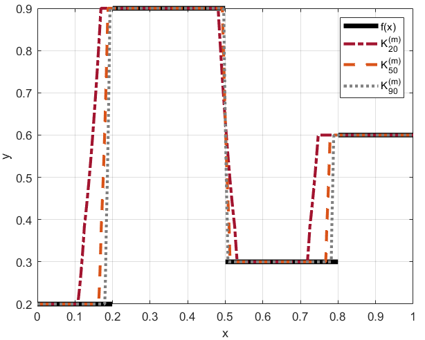
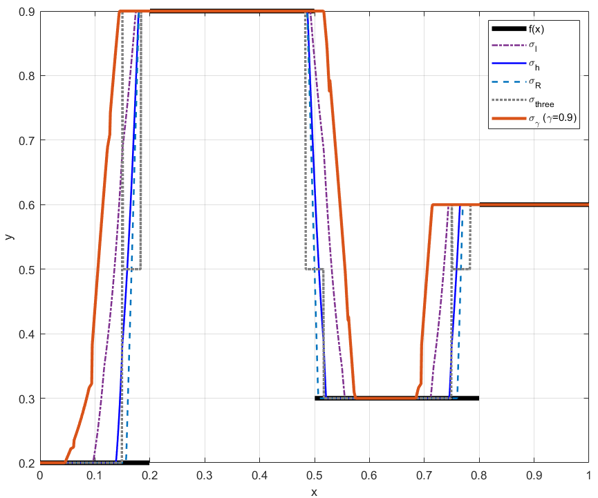
Figure 1. Left: Approximation quality of Kantorovich type max-min operator $K_{n}^{(m)}(f)$ for increasing sampling rate $n$. Right: Approximation of $f$ by $K_{30}^{(m)}(f)$ using different sigmoidal functions.

Choosing $\sigma=\sigma_{h}$, the approximation by the Kantorovich type max-min operator $K_{n}^{\left(m\right)}\left(f\right)$ is illustrated in Figure 1 (left) for increasing values of $n$. For the discontinuous function $f$ it gets visible that point-wise convergence at the discontinuity points can in general not be expected, but that $L^{p}$-convergence of $K_{n}^{\left(m\right)}\left(f\right)$ towards $f$ is available. This is confirmed theoretically by Theorem 3.4 and gets also apparent from the listed $L^{1}$-errors in Table 5. In order to give a broader picture about the approximation behavior of the different kernels to the reader, we compare also the five introduced sigmoidal functions ($\sigma_{l},\sigma_{h},\sigma_{R},\sigma_{three},\sigma_{\gamma}$) for the approximation of the same function $f$ taking $n=30$ sampling points. The respective result is visualized in Figure 1 (right).

Comparison with max-product and linear neural network operators. In a next step, we want to compare the Kantorovich type max-min operator with the Kantorovich variants of the max-product and the linear neural network operators that are given as

$$K_{n}^{\left(M\right)}\left(f;x\right):=\bigvee\limits_{k=\left\lceil na\right\rceil}^{\left\lfloor nb\right\rfloor-1}n\int\limits_{\frac{k}{n}}^{\frac{k+1}{n}}f\left(u\right)du\dfrac{\phi_{\sigma}\left(nx-k\right)}{\bigvee\limits_{d=\left\lceil na\right\rceil}^{\left\lfloor nb\right\rfloor-1}\phi_{\sigma}\left(nx-d\right)}\text{ \ \ (see \cite[cite]{[\@@bibref{}{cost25}{}{}]})}$$

and

$$K_{n}\left(f;x\right):=\sum\limits_{k=\left\lceil na\right\rceil}^{\left\lfloor nb\right\rfloor-1}n\int\limits_{\frac{k}{n}}^{\frac{k+1}{n}}f\left(u\right)du\dfrac{\phi_{\sigma}\left(nx-k\right)}{\sum\limits_{d=\left\lceil na\right\rceil}^{\left\lfloor nb\right\rfloor-1}\phi_{\sigma}\left(nx-d\right)}\text{ \ (see \cite[cite]{[\@@bibref{}{cost4}{}{}]})}$$

respectively. Taking these operators into account using the hyperbolic tangent sigmoidal function $\sigma=\sigma_{h}$, we get the approximation errors in the space $L^{1}\left(\left[0,1\right],\left[0,1\right]\right)$ listed in Table 5 and Figure 2 (left). It can be seen, that the Kantorovich variants of all three neural network operators behave very similarly in terms of the approximation error with the max-product variant having a slightly better performance than the max-min and the classical linear variant. On the other hand, if we compare the computational time of the operation, the max-min and max-product operators clearly outperform the classical operator for sampling numbers $n>660$ (see Figure 2 (right)).

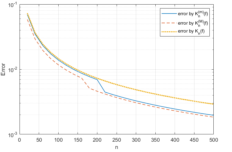
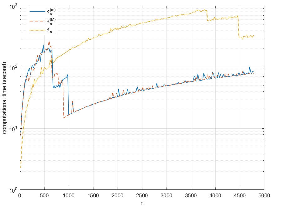
Figure 2. Left: errors for the approximation of the function $f$ in $L^{1}\left(\left[0,1\right],\left[0,1\right]\right)$ by $K_{n}^{(m)}(f),K_{n}^{(M)}(f)$ and $K_{n}(f)$. Right: Comparison of the computational times to calculate the functions $K_{n}^{(m)}(f)$, $K_{n}^{(M)}(f)$ and $K_{n}(f)$.

100.14570.13860.1171300.04850.04620.0390900.01620.01540.01301500.00970.00920.00785000.00290.00200.0018Table 5: Comparison of approximation errors of Kantorovich type neural network operators\overset{\text{{Table \ref{table1}: }Comparison of approximation errors of\ Kantorovich type neural network operators}\ }{\begin{tabular}[c]{cccc}\hline\cr\hline\cr$n$&$||K_{n}\left(f\right)-f||_{1}$&$||K_{n}^{\left(m\right)}\left(f\right)-f||_{1}$&$||K_{n}^{\left(M\right)}\left(f\right)-f||_{1}$\\ \hline\cr\hline\cr$10$&0.1457&0.1386&0.1171\\ \hline\cr$30$&0.0485&0.0462&0.0390\\ \hline\cr$90$&0.0162&0.0154&0.0130\\ \hline\cr$150$&0.0097&0.0092&0.0078\\ \hline\cr$500$&0.0029&0.0020&0.0018\\ \hline\cr\hline\cr\end{tabular}\ \ \ }

n‖-Kn(f)f‖1‖-Kn(m)(f)f‖1‖-Kn(M)(f)f‖1

Application to signal denoising and ECG signal filtering. We finally provide some applications of the Kantorovich type max-min operators to signal denoising. The incorporation of the Kantorovich information in the max-min operator can be interpreted as a pre-processing step of the actual max-min approximation in which a preliminary linear convolution filter is applied to the initial signal. In general, this preliminary filtering allows for an additional noise reduction and a smoothing of the signal.

To see the denoising benefits of the Kantorovich variant $K_{n}^{(m)}(f)$ compared to the classical sampling variant $F_{n}^{(m)}(f)$ of the neural network operator, we apply both variants to the discontinuous test function $f$ introduced above equipped with additional normally distributed Gaussian noise. Using $n=8000$ samples and a suitable scaled kernel $\phi_{\sigma_{l}}(0.1x)$ based on the logistic sigmoidal function $\sigma_{l}$, the corresponding results are illustrated in Figure 3. In order to approximate the local integrals of the noisy function and to calculate the Kantorovich information, we used a Riemann sum based on additional refined samples of the signal. With other quadrature rules as the trapezoidal rule, similar results were obtained. It is visible that the usage of the Kantorovich information of the signal instead of point evaluations leads to an improved denoising of the noisy signal.

Figure 3. Top row: original signal $f$ (left) and signal $f$ equipped with Gaussian noise (right). Bottom row: Kantorovich variant $K_{n}^{(m)}(f)$ (left) compared to the classical max-min variant $F_{n}^{(m)}(f)$ (right) of the max-min neural network operator applied to the noisy signal.

For another comparison between the operators $K_{n}^{(m)}$ and $K_{n}^{(M)}$, we apply both on an ECG signal describing $5$ heart beats (using $n=1600$ time samples) of patient 101 taken from the MIT-BIH Arrhythmia Database [42]. Here we use the mean value of two consecutive time samples to approximate the Kantorovich information and apply the operators $K_{n/2}^{(m)}$ and $K_{n/2}^{(M)}$ to the ECG signal with the kernel $\phi_{\sigma_{l}}(2x)$.

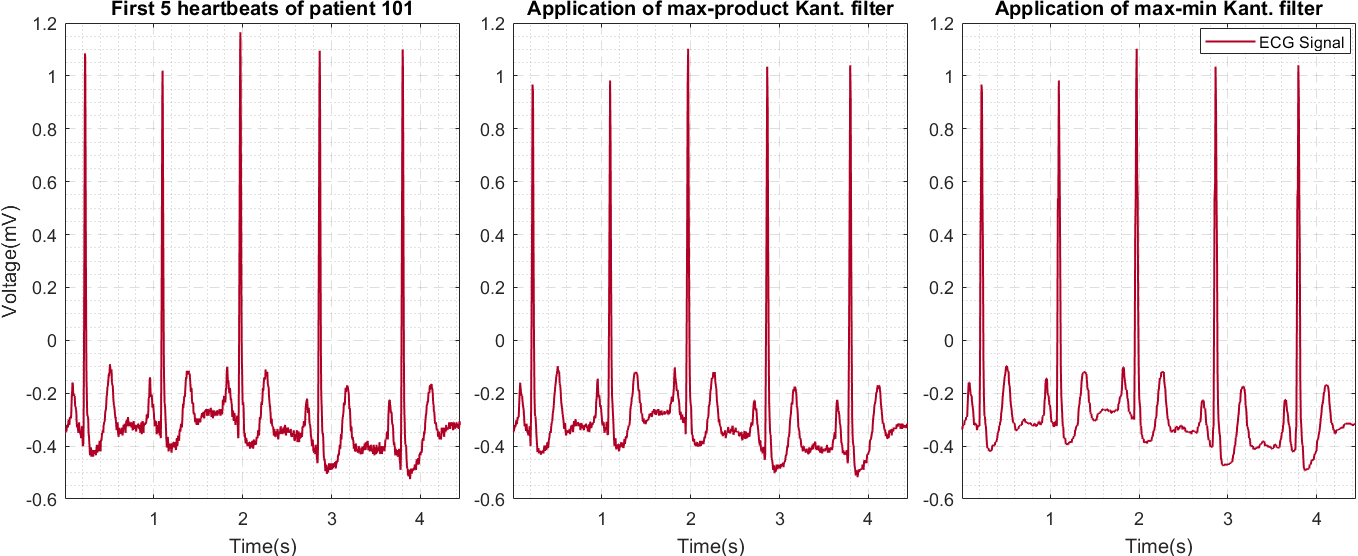
Figure 4. Comparison of the Kantorovich forms of the max-min and max-product Neural Network operators

Both operators provide denoised approximations of the ECG signal, the max-min Kantorovich variant having stronger smoothing effects, as shown in Figure 4.

6. Concluding Remarks

In this study, we investigated the Kantorovich variant of the max-min neural network operators, analysing its convergence and approximation properties in the $L^{p}$-spaces in more detail. In addition, we included some numerical examples to underpin the theoretical results and to outline possible practical applications of the operators for the denoising of biomedical signals. Our experiments demonstrate that max-min Kantorovich form of the network operators achieve superior results in denoising compared to their max-product counterparts. In the future, we aim to study the $N$-dimensional cases of these neural network operators, enabling us to analyze and process not only images but also higher-dimensional datasets.

7. Acknowledgements

The first author was funded by the Scientific and Technological Research Council of Türkiye (TÜBİTAK). The second and third author were funded by GNCS-IN$\delta$AM and the European Union - NextGenerationEU under the National Recovery and Resilience Plan (NRRP), Mission 4 Component 2 Investment 1.1 - Call PRIN 2022 No. 104 of February 2, 2022 of Italian Ministry of University and Research; Project 2022FHCNY3 (subject area: PE - Physical Sciences and Engineering) ”Computational mEthods for Medical Imaging (CEMI)”. We also thank the Italian Network on Approximation (RITA) and the topical group on “Approximation Theory and Applications” of the Italian Mathematical Union.

İsmail Aslan

Hacettepe University

Department of Mathematics,

Çankaya TR-06800, Ankara, Türkiye

E-mail: ismail-aslan@hacettepe.edu.tr

Stefano De Marchi

University of Padova

Department of Mathematics “Tullio Levi-Civita”,

Via Trieste 63, 35121 Padova, Italy

E-mail: stefano.demarchi@unipd.it

Wolfgang Erb

University of Padova

Department of Mathematics “Tullio Levi-Civita”,

Via Trieste 63, 35121 Padova, Italy

E-mail: wolfgang.erb@unipd.it

References

- [1] Anastassiou, G. A. (2011). Multivariate sigmoidal neural network approximation. Neural Networks, 24(4), 378-386.
- [2] Anastassiou, G. A. (2011). Intelligent systems reference library: vol. 19. Intelligent systems: approximation by artificial neural networks, Berlin: Springer-Verlag.
- [3] Anastassiou, G. A. (2011). Multivariate hyperbolic tangent neural network approximation. Computers & Mathematics with Applications, 61(4), 809-821.
- [4] Anastassiou, G. A. (2011). Univariate hyperbolic tangent neural network approximation. Mathematical and Computer Modelling, 53(5-6), 1111-1132.
- [5] Anastassiou, G. A. (2012). Univariate sigmoidal neural network approximation. Journal of Computational Analysis & Applications, 14(1), 659-690.
- [6] Anastassiou, G. A. (2019). Approximation by multivariate sublinear and max-product operators. Revista de la Real Academia de Ciencias Exactas, Físicas y Naturales. Serie A. Matemáticas, 113, 507-540.
- [7] Aslan, I. (2024). Approximation by Max-Min Neural Network Operators. (submitted for publication).
- [8] Bede, B., Coroianu, L., & Gal, S. G. (2009). Approximation and shape preserving properties of the Bernstein operator of max-product kind. International journal of mathematics and mathematical sciences, 2009.
- [9] Bede, B., Coroianu, L., & Gal, S. G. (2010). Approximation and shape preserving properties of the nonlinear Favard-Szasz-Mirakjan operator of max-product kind. Filomat, 24(3), 55-72.
- [10] Bede, B., Coroianu, L., & Gal, S. G. (2016). Approximation by max-product type operators. Heidelberg: Springer.
- [11] Bede, B., Nobuhara, H., Daňková, M., & Di Nola, A. (2008). Approximation by pseudo-linear operators. Fuzzy Sets and Systems, 159(7), 804-820.
- [12] Bede, B., Schwab, E. D., Nobuhara, H., & Rudas, I. J. (2009). Approximation by Shepard type pseudo-linear operators and applications to image processing. International journal of approximate reasoning, 50(1), 21-36.
- [13] Butzer, P. L., & Berens, H. (2013). Semi-groups of operators and approximation (Vol. 145). Springer Science & Business Media.
- [14] Costarelli, D, (2014). Sigmoidal functions approximation and applications (Ph.D. thesis), Roma Tre University, Rome, Italy.
- [15] Costarelli, D., & Sambucini, A. R. (2018). Approximation results in Orlicz spaces for sequences of Kantorovich max-product neural network operators. Results in Mathematics, 73(1), 15.
- [16] Costarelli, D., Sambucini, A. R., & Vinti, G. (2019). Convergence in Orlicz spaces by means of the multivariate max-product neural network operators of the Kantorovich type and applications. Neural Computing and Applications, 31(9), 5069-5078.
- [17] Costarelli, D., & Spigler, R. (2013). Approximation results for neural network operators activated by sigmoidal functions. Neural Networks, 44, 101-106.
- [18] Costarelli, D., & Spigler, R. (2013). Multivariate neural network operators with sigmoidal activation functions. Neural Networks, 48, 72-77.
- [19] Costarelli, D., & Spigler, R. (2014). Convergence of a family of neural network operators of the Kantorovich type. Journal of Approximation Theory, 185, 80-90.
- [20] Costarelli, D., & Vinti, G. (2016). Max-product neural network and quasi-interpolation operators activated by sigmoidal functions. Journal of Approximation Theory, 209, 1-22.
- [21] Costarelli, D., & Vinti, G. (2016). Approximation by max-product neural network operators of Kantorovich type. Results in Mathematics, 69, 505-519.
- [22] Costarelli, D., & Vinti, G. (2016). Pointwise and uniform approximation by multivariate neural network operators of the max-product type. Neural Networks, 81, 81-90.
- [23] Costarelli, D., & Vinti, G. (2017). Saturation classes for max-product neural network operators activated by sigmoidal functions. Results in Mathematics, 72, 1555-1569.
- [24] Costarelli, D., & Vinti, G. (2018). Estimates for the neural network operators of the max-product type with continuous and p-integrable functions. Results in Mathematics, 73, 1-10.
- [25] Costarelli, D., & Vinti, G. (2019). Quantitative estimates involving K-functionals for neural network-type operators. Applicable Analysis, 98(15), 2639-2647.
- [26] Cantarini, M., Coroianu, L., Costarelli, D., Gal, S. G., & Vinti, G. (2021). Inverse result of approximation for the max-product neural network operators of the Kantorovich type and their saturation order. Mathematics, 10(1), 63.
- [27] Cardaliaguet, P., & Euvrard, G. (1992). Approximation of a function and its derivative with a neural network. Neural networks, 5(2), 207-220.
- [28] Cheang, G. H. (2010). Approximation with neural networks activated by ramp sigmoids. Journal of Approximation Theory, 162(8), 1450-1465.
- [29] Chen, Z., & Cao, F. (2009). The approximation operators with sigmoidal functions. Computers & Mathematics with Applications, 58(4), 758-765.
- [30] Chen, Z., & Cao, F. (2012). The construction and approximation of a class of neural networks operators with ramp functions. Journal of Computational Analysis and Applications, 14(1), 101-112.
- [31] Coroianu, L., Costarelli, D., & Kadak, U. (2022). Quantitative estimates for neural network operators implied by the asymptotic behaviour of the sigmoidal activation functions. Mediterranean Journal of Mathematics, 19(5), 211.
- [32] Coroianu, L., Costarelli, D., Gal, S. G., & Vinti, G. (2019). The max-product generalized sampling operators: convergence and quantitative estimates. Applied Mathematics and Computation, 355, 173-183.
- [33] Coroianu, L., & Gal, S. G. (2018). Approximation by truncated max-product operators of Kantorovich-type based on generalized ()-kernels. Mathematical Methods in the Applied Sciences, 41(17), 7971-7984.
- [34] Coroianu, L., & Gal, S. G. (2022). New approximation properties of the Bernstein max-min operators and Bernstein max-product operators. Mathematical Foundations of Computing, 5(3), 259-268.
- [35] Duman, O. (2016). Nonlinear Approximation: q-Bernstein Operators of Max-Product Kind. In Intelligent Mathematics II: Applied Mathematics and Approximation Theory (pp. 33-56). Springer International Publishing.
- [36] Duman, O. (2024). Max-product Shepard operators based on multivariable Taylor polynomials. Journal of Computational and Applied Mathematics, 437, 115456.
- [37] Gökçer, T. Y., & Aslan, İ. (2022). Approximation by Kantorovich-type max-min operators and its applications. Applied Mathematics and Computation, 423, 127011.
- [38] Gökçer, T. Y., & Duman, O. (2020). Approximation by max-min operators: A general theory and its applications. Fuzzy Sets and Systems, 394, 146-161.
- [39] Gökçer, T. Y., & Duman, O. (2022). Regular summability methods in the approximation by max-min operators. Fuzzy Sets and Systems, 426, 106-120.
- [40] Holhoş, A. (2018). Weighted approximation of functions by Meyer–König and Zeller operators of max-product type. Numerical Functional Analysis and Optimization, 39(6), 689-703.
- [41] Kadak, U. (2022). Multivariate neural network interpolation operators. Journal of Computational and Applied Mathematics, 414, 114426.
- [42] Moody, G. B., Mark, R. G. (2001). The impact of the MIT-BIH Arrhythmia Database. IEEE Eng. in Med. and Biol., 20(3), 45-50
- [43] Peetre, J. (1970). A new approach in interpolation spaces. Studia Mathematica, 34(1), 23-42.
- [44] Yüksel Güngör, Ş., & İspir, N. (2018). Approximation by Bernstein-Chlodowsky operators of max-product kind. Mathematical Communications, 23(2), 205-225.