Dynamics of An Information Theoretic Analog of Two Masses on a Spring

Abstract

In this letter we investigate an information theoretic analogue of the classic two masses on spring system, arising from a physical interpretation of Friston’s free energy principle in the theory of learning in a system of agents. Using methods from classical mechanics on manifolds, we define a kinetic energy term using the Fisher metric on distributions and a potential energy function defined in terms of stress on the agents’ beliefs. The resulting Lagrangian (Hamiltonian) produces a variation of the classic DeGroot dynamics. In the two agent case, the potential function is defined using the Jeffrey’s divergence and the resulting dynamics are characterized by a non-linear spring. These dynamics produce trajectories that resemble flows on tori but are shown numerically to produce chaos near the boundary of the space. We then investigate persuasion as an information theoretic control problem where analysis indicates that manipulating peer pressure with a fixed target is a more stable approach to altering an agent’s belief than providing a slowly changing belief state that approaches the target.

The free energy principle was developed by Friston, Kilner and Harrison [1] as a thermodynamically inspired model of perception that presupposes the brain minimizes surprise (entropy) by maintaining an internal model of reality that is updated regularly through sensory input. Connections between this work, statistical mechanics and nonlinear dynamics have been subsequently studied by Friston and others [2, 3, 4, 5, 6, 7, 8, 9, 10, 11, 12] and extended to more generic biological systems [13] as well as machine learning contexts [14]. More recently, Hein et al. [15] showed that the principle of “surprise minimization” allows for collective behavior to arise in complex interacting systems.

In this letter, we rephrase the free energy principle in terms of free entropy, which arises naturally from the information geometry of the Fisher metric [16, 17, 18]. This quantity and the corresponding techniques from information geometry have been used extensively in statistical physics [19, 20, 21, 22, 23, 24, 25, 26, 27].

Using techniques from classical mechanics on manifolds, we derive an alternative to the DeGroot averaging model (see e.g., [28, 29, 30]), which has similar structure and properties but emerges naturally from our information theoretic variation of the free energy principle as a classical mass/spring system, further supporting the hypothesis that “surprise minimization” can lead to collective behavior [15]. In this derivation, a statistical divergence replaces the classical square distance in the Hooke spring potential. Convergence to an opinion is ensured by the inclusion of a dissipative “dashpot” term [31, 32] and consensus is determined by the spring constants. While opinion dynamics have been studied extensively [33, 34, 35, 36, 37, 38, 39, 40, 41, 42, 43, 44, 45, 46, 47, 48] along with the related disciplines of flocking and consensus [33, 34, 49, 50, 51, 52, 53, 54, 55, 56, 30], we believe this is the first derivation of these dynamics from the free energy principle or the corresponding “minimum surprise principle” rephrased as a free entropy minimization.

Let $p(\mathbf{x}|\bm{\eta})$ be a probability distribution parameterized by $\bm{\eta}$. For two distributions $p(\mathbf{x}|\bm{\eta})$ and $q(\mathbf{x}|\bm{\eta})$, the Kullback-Liebler divergence is given by,

$$D_{KL}(p|q)=\int_{X}p(\mathbf{x}|\bm{\eta})\ln\left(\frac{p(\mathbf{x}|\bm{\eta})}{q(\mathbf{x}|\bm{\eta})}\right)d\mathbf{x}.$$ (1)

It is straightforward to see that the KL-divergence is neither symmetric nor does it satisfy any version of the triangle inequality [57]. Likewise, the quadratic form of the Fisher metric is defined componentwise as,

$$g_{ij}(\bm{\eta})=\int_{X}\frac{\partial\log\left[p(\mathbf{x}|\bm{\eta})\right]}{\partial x_{i}}\frac{\partial\log\left[p(\mathbf{x}|\bm{\eta})\right]}{\partial x_{j}}p(\mathbf{x}|\bm{\eta})\,dx.$$

Unlike Euclidean spaces, statistical manifolds admit divergences, which are locally consistent with the Fisher metric, but are themselves not true distances. The Kullbach-Liebler divergence, already introduced, is one such divergence. In particular, we can locally write,

$$D_{KL}\left[p(\mathbf{x}|\bm{\eta})|p(\mathbf{x}|\bm{\eta}_{0})\right]=\\ \frac{1}{2}\mathbf{g}_{jk}(\bm{\eta}_{0})\Delta\eta_{0}^{j}\Delta\eta_{0}^{k}+O(\left\lVert\bm{\Delta\eta}_{0}\right\rVert^{3}),$$

showing the relationship between the metric and the divergence [57].

Using the kinetic energy, computed using the Fisher metric, we can form a Lagrangian

$$L(\bm{\eta},\dot{\bm{\eta}})=\frac{1}{2}\mathbf{g}_{jk}(\bm{\eta})\dot{\eta}^{j}\dot{\eta}^{k}-V(\bm{\eta)},$$ (2)

where $V$ is a potential function, to be defined in context.

Let $\Delta_{n-1}$ be the $n-1$ dimensional unit simplex embedded in $\mathbb{R}^{n}$. The categorical distribution with parameters $q^{1},\dots,q^{n-1}$ is the vector $(q^{0},\dots,q^{n-1})\in\Delta_{n-1}$, where

$$q^{0}=1-\sum_{j}q^{j}.$$ (3)

In this case, the metric tensor can be computed explicitly as $g_{ij}=\delta_{ij}/{q^{i}}+1/q^{0},$ where $1\leq i,j\leq n-1$.

Consider the two outcome (Bernoulli) case and let $q^{1}=q$ and $q^{0}=1-q$. Then the kinetic energy is,

$$T(q)=\frac{m}{2}\frac{\dot{q}^{2}}{q(1-q)}.$$ (4)

Here, $m$ is a mass term that could be unitized.

For the remainder of this paper, we consider the setting where $q$ is the parameter in a Bernoulli random variable representing an agent’s belief about a certain outcome or opinion about a certain bivalent topic. If $q^{\prime}\in(0,1)$ is a fixed belief point (i.e., an external reference point) then the Kullbach-Liebler divergence yields an information theoretic “squared distance” from $q$ to $q^{\prime}$ as,

$$D(q,q^{\prime})=q\log\left(\frac{q}{q^{\prime}}\right)+(1-q)\log\left(\frac{1-q}{1-q^{\prime}}\right).$$

In this scenario $q^{\prime}$ is treated as a prior belief and $q$ is treated as a posterior belief. Mimicking the potential energy for a spring, and using Eq. 2 and Eq. 4, the Lagrangian written in terms of $q$, $\dot{q}$, and $q^{\prime}$ is,

$$L(q,q^{\prime})=\frac{m}{2}\frac{\dot{q}^{2}}{q(1-q)}-\frac{k}{2}D(q,q^{\prime}),$$

where we assume (for now) that $q^{\prime}$ represents a fixed Bernoulli distribution and $k$ is a notional spring constant. This has corresponding Hamiltonian,

$$H(q,p)=\frac{q(1-q)}{2m}p^{2}+\frac{k}{2}D(q,q^{\prime}),$$

where,

$$\frac{\partial L}{\partial\dot{q}}=p=\frac{m\dot{q}}{q(1-q)},$$

is the conjugate momentum variable. Expanding to second order around $q=q^{\prime}=\tfrac{1}{2}$, $H(q,p)$ has form,

$$H(q,p)=\frac{q(1-q)}{2m}p^{2}+k(q-q^{\prime})^{2}+O(q^{3}),$$

showing that this is just a nonlinear spring potential.

Using the foregoing analysis, we can derive a variant of the DeGroot dynamics [29, 58, 30]. As before, let $q_{i}$ be the parameter in a Bernoulli random variable representing an agent’s belief about a certain outcome or opinion about a certain bivalent topic. Let $k_{ij}$, be a spring constant, denoting the degree to which agent $i$ and agent $j$ influence each other’s belief and let $q_{i}^{\prime}$ be a prior belief held by agent $i$ with a restoring force $k_{i}$. Then the Hamiltonian for this system in canonical coordinates is given by,

$$H(\mathbf{q},\mathbf{p})=\sum_{i}\frac{q_{i}(1-q_{i})}{2m_{i}}p_{i}^{2}+\sum_{i}\frac{k_{i}}{2}\left(q_{i}-q^{\prime}_{i}\right)^{2}+\\ \sum_{i<j}\frac{k_{ij}}{2}\left(q_{i}-q_{j}\right)^{2}+O\left(\left\lVert\bm{q}\right\rVert^{3}\right).$$ (5)

Assuming each agent experiences stress from an opinion that differs from a fixed (or prior) opinion $q^{\prime}_{i}$, the standard DeGroot Hamiltonian (stress function) [29, 58, 30] is similar,

$$H_{D}(\mathbf{q})=\sum_{i}\frac{k_{i}}{2}\left(q_{i}-q^{\prime}_{i}\right)^{2}+\sum_{i<j}\frac{k_{ij}}{2}\left(q_{i}-q_{j}\right)^{2}.$$ (6)

Under most circumstances, $q_{i}^{\prime}$ is the initial belief of the agent, although it can represent any fixed belief that influences the agent. The repeated averaging dynamics [29, 30] are derived by differentiating $H_{D}$ with respect to $q_{i}$ and solving for the local minimum. Agents then update their belief to the local minimum. Alternatively, Gavrilets et al. [59] assumes a Jacobi iteration so that, $\dot{q}_{i}=-\frac{\partial H_{D}}{\partial q_{i}},$ which is consistent with the consensus dynamics literature (see [56] for an overview).

A modification to the stress function that is consistent with the free energy hypothesis [1] is to assume that the stress of internal model adjustment occurs continuously, rather than from a fixed initial assumption. This adds an additional term to Eq. 6,

$$\hat{H}_{D}(\mathbf{q})=\sum_{i}\frac{\hat{k}_{i}(\epsilon)}{2}\left[q_{i}(t+\epsilon)-q_{i}(t)\right]^{2}\\ +\sum_{i}\frac{k_{i}}{2}\left(q_{i}-q^{\prime}_{i}\right)^{2}+\sum_{i<j}\frac{k_{ij}}{2}\left(q_{i}-q_{j}\right)^{2},$$ (7)

and allows the stress contributed by the initial belief to be disregarded (by setting $k_{i}=0$) while still producing transitive dynamics. If $\hat{k}_{i}(\epsilon)\propto 1/\epsilon$ then we recover the form of Eq. 5 from Eq. 7 as $\epsilon\to 0$.

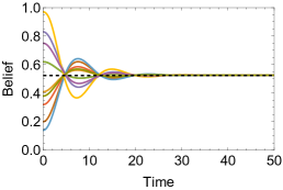
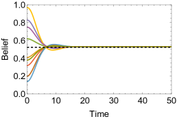
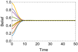
Figure 1: When $k_{i}=0$ for all $i$, agents converge to consensus as a result of increasing peer-pressure in the dissipative system. Prior to convergence, the dynamics oscillate consistent with Fink et al.’s theory of oscillating belief. (Left) $\alpha=0.35$. (Center) $\alpha=0.6$. (Right) $\alpha=0.75$. The mean of the initial conditions is shown as a dashed line.

The dynamics of Eq. 5 and Eq. 6 are fundamentally different. The kinetic energy term causes belief oscillation (discussed in detail in the sequel), while this is not observed in long-run human behavior (though may be expected in the short term [60]), with convergence to a consensus opinion expected over time. We can recover such dynamics by introducing a dissipative element to the Lagrangian used to generate Eq. 5. As in [32], let,

$$\tilde{L}(q,q^{\prime})=e^{-\alpha t}\left[\frac{m}{2}\frac{\dot{q}^{2}}{q(1-q)}-\frac{k}{2}D(q,q^{\prime})^{2}\right].$$

Then the Hamiltonian of the system becomes,

$$\tilde{H}(q,q^{\prime})=e^{-\alpha t}\frac{q(1-q)}{2m}p_{i}^{2}+e^{\alpha t}\frac{k}{2}D(q,q^{\prime})^{2}.$$

Passing to the general case, our proposed model is,

$$\tilde{H}(\mathbf{q},\mathbf{p})=e^{-\alpha t}\sum_{i}\frac{q_{i}(1-q_{i})}{2m_{i}}p_{i}^{2}+\\ e^{\alpha t}\left[\sum_{i}\frac{k_{i}}{2}D(q_{i},q_{i}^{\prime})+\sum_{i\neq j}\frac{k_{ij}}{2}D(q_{i},q_{j})\right].$$ (8)

Like the repeated averaging DeGroot model with increasing peer-pressure [29, 58, 30], this system converges to consensus when $k_{i}=0$ for all $i$; that is, when there are no external spring forces outside of the agents’ beliefs. The oscillating behavior for smaller values of $\alpha$ is consistent with some theories of human cognition (see Fink et al. [61, 60] and their references), which assert that beliefs will oscillate, going so far as to use a spring analogy. Convergence to consensus is illustrated in Fig. 1 for varying values of $\alpha$. It is worth noting that when $\alpha$ is small, convergence does not necessarily occur to a weighted mean of the initial conditions, as it does in the work of Gavrilets et al. [59] and in Griffin et al. [29, 58, 30].

Notably when $k_{i}>0$ for some $i$, the inclusion of fixed external belief forces implies that consensus is not ensured, even though the agents converge to fixed beliefs, as is expected for a dissipative system. This is shown in Fig. 2, where $k_{i}=0.3$ for all $i$.

Figure 2: When $k_{i}>0$ for some $i$, consensus is not ensured and agents will converge to non-consensus states. Here $\alpha=0.5$ and $k_{i}=0.3$ for all $i$. The mean of the initial conditions is shown as a dashed line.

For practical modeling purposes, we expect the mass terms $m_{i}$ and $\alpha$ to be comparatively large, explaining why decision makers are slow to make changes to their mental models and do not oscillate substantially in their beliefs. This reduces the kinetic energy component of the Hamiltonian, thus making the model much more like the DeGroot model with an increasing peer-pressure term as in [30]. Notably the dissipative multiplier is equivalent to assuming jointly increasing peer-pressure and decreasing mass. Nevertheless, it is worth studying the Hamiltonian dynamics in non-dissipative systems as an interesting example of a nonlinear spring-mass system in an unusual geometry. This investigation can also provide insight into transient belief dynamics.

Consider the two-agent Hamiltonian,

$$H(\mathbf{q},\mathbf{p})=\frac{1}{2}q_{1}(1-q_{1})p_{1}^{2}+\frac{1}{2}q_{2}(1-q_{2})p_{2}^{2}+\\ \frac{k}{2}D_{J}(q_{1},q_{2}),$$ (9)

where mass constants are unitized for simplicity and $D_{j}(q_{1},q_{2})$ is the Jeffrey’s divergence,

$$D_{J}(q_{1},q_{2})=D(q_{1},q_{2})+D(q_{2},q_{1}).$$

This is a classic two-mass spring system in a non-Euclidean geometry. In the Euclidean case, it is easy to see the resulting dynamics are integrable and admit two constants of motion, the energy (given by the corresponding Hamiltonian) and the linear momentum of the total system. In contrast, we can show numerically that the Hamiltonian dynamics in Eq. 9 are not integrable, showing signs of weak chaos [62].

Introduce the canonical coordinate transform,

$$q_{i}=\cos^{2}\left(\frac{\theta_{i}}{2}\right)\qquad i\in\{1,2\}.$$ (10)

Then Eq. 9 becomes a classical non-linear spring Hamiltonian with two coupled masses,

$$H(\bm{\theta},\bm{\omega})=\frac{p_{1}^{2}}{2}+\frac{p_{2}^{2}}{2}+\frac{k}{4}\left[\cos(\theta_{1})-\cos(\theta_{2})\right]\log\left[\frac{\tan^{2}\left(\frac{\theta_{2}}{2}\right)}{\tan^{2}\left(\frac{\theta_{1}}{2}\right)}\right].$$ (11)

As expected and consistent with Eq. 5, the second order approximation for this is,

$$H_{0}(\bm{\theta},\bm{\omega})=\frac{p_{1}^{2}}{2}+\frac{p_{2}^{2}}{2}+\frac{k}{2}(\theta_{1}-\theta_{2})^{2}+O(\left\lVert\bm{\theta}\right\rVert^{3}).$$ (12)

Consequently, we can express $H(\bm{\theta},\bm{\omega})$ as,

$$H(\bm{\theta},\bm{\omega})=H_{0}(\bm{\theta},\bm{\omega})+\epsilon H_{1}(\bm{\theta},\bm{\omega}),$$

where $H_{0}$ is an integrable Hamiltonian, $\epsilon$ is a perturbation constant and $H_{1}$ is the nonlinear Hamiltonian perturbation. Since the coordinate transform in Eq. 10 is a diffeomorphism, we may expect to see Hamiltonian chaos arise in the dynamics generated by Eq. 9. We find evidence for weak chaos [62] associated to behavior near the manifold boundary. This is shown in Fig. 3, where we see a decaying estimate for the maximum Lyapunov exponent, followed by a slight increase, using the Wolf algorithm [63]. In Fig. 3, $k=2$, which improves numerical stability of the long trajectory required to execute the Wolf algorithm. The fact that the maximum Lyapunov exponent is positive and the dynamics play out on a compact set is sufficient to conclude that they are (weakly) chaotic.

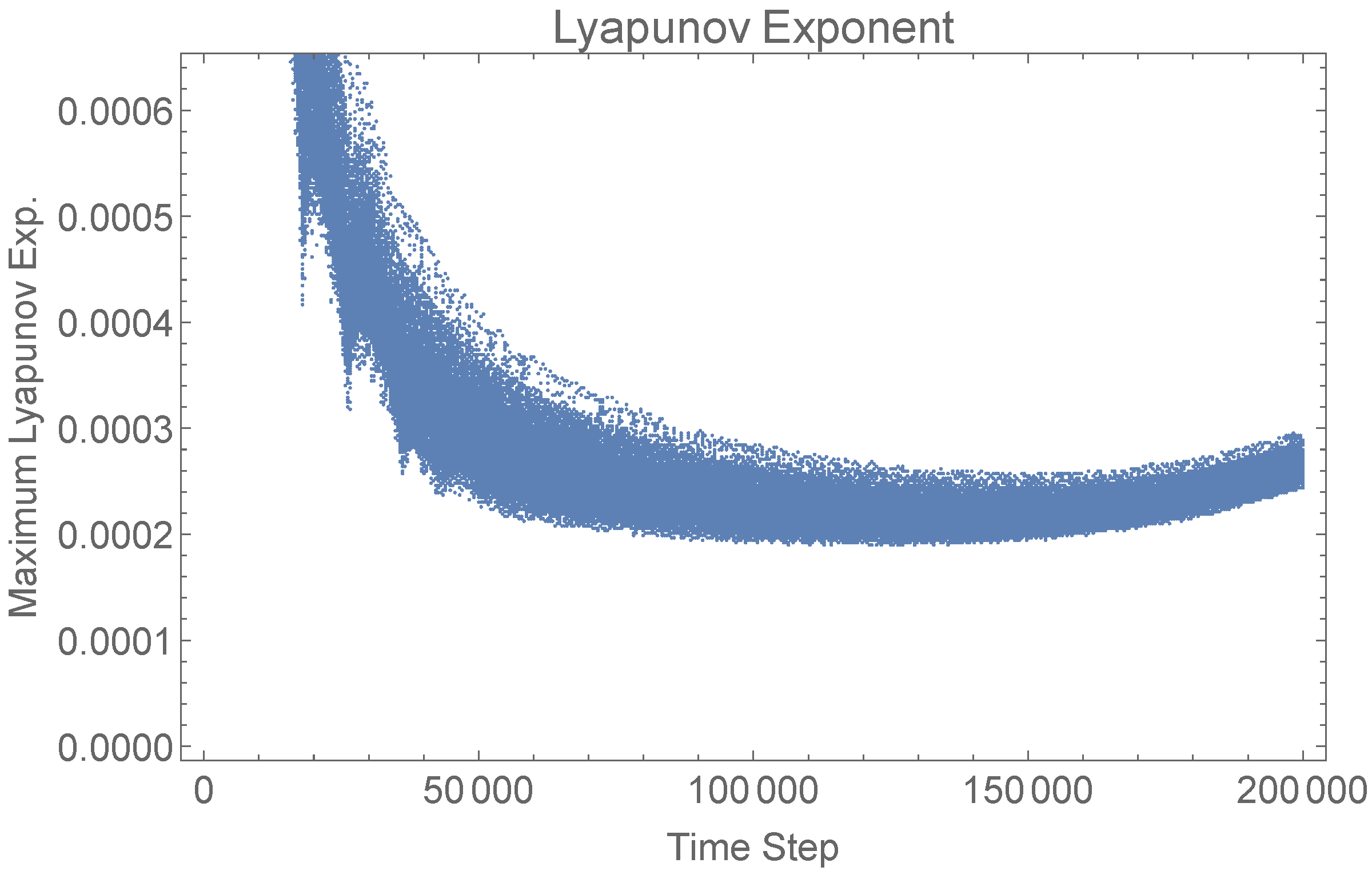
Figure 3: The Wolf algorithm [63] is used to estimate the Lyapunov spectrum for the Hamiltonian dynamics arising from Eq. 9. The results suggest weak chaos caused by behavior near the boundaries of the space.

This is consistent with prior results on Hamiltonian chaos on compact sets defined by the unit simplex that showed that the chaotic dynamics arose as a result of interactions with the boundary [64]. This Hamiltonian system is unusual in that it has an infinite line of fixed points $q_{1}=q_{2}$ and $p_{1}=p_{2}=0$. The result is a degeneracy, which makes application of the classical KAM theorem impossible [65] because the dynamics generated by $H_{0}$ evolve on a cylinder homeomorphic to $\mathbb{S}^{1}\times\mathbb{R}$, rather than the two-torus $\mathbb{S}^{2}$. From this we see that sensitivity to initial conditions and the classical behaviors associated to weak chaos emerge as a result of asymmetries in the initial conditions. This is shown in Fig. 4, where we fix $q_{2}(0)=\tfrac{1}{2}$ and vary $q_{1}(0)$, illustrating the distinct trajectory structures that emerge.

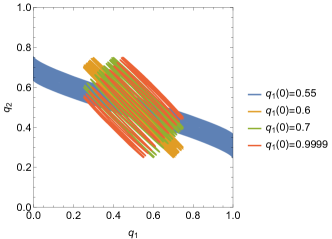
Figure 4: As $q_{1}(0)$ is varied, the structure of the trajectory $(q_{1},q_{2})$ changes from an ellipse to a complex curve.

Despite the results of the Wolf algorithm, the trajectories in Fig. 4 seem well-behaved. This is because of the region in the interior of unit simplex, where the geometry is locally Euclidean. In this region, the behavior of the system is given almost entirely by a two-mass and spring system. Non-integrability (and thus the destruction of additional conserved quantities) is only introduced when the dynamics interact with the boundary, which induces an effective nonlinear force, not present in Euclidean space.

The introduction of nonlinear forces from the geometry of the space itself has implications for the corresponding control problem, which can provide insights into understanding persuasion in bivalent topics [66]. Of particular interest is the question of whether an external belief (i.e., perceived evidence) or its associated spring constant (i.e., social pressure) are more effective control parameters.

Formally stated, given a binary belief in $\theta$-coordinates and an initial belief $\theta_{0}$, the goal is to use either an external belief $\theta^{\prime}$ or the associated spring constant $k$ to move $\theta$ to a desired target $\theta_{f}$ in time horizon $T$ while minimizing the objective function,

$$\mathcal{O}=\min\int_{t_{0}}^{t_{f}}\frac{p^{2}}{2}+Cdt,$$ (13)

where $C$ is a cost associated to the control parameter. We include the kinetic energy term in the performance index because without some cost associated to momentum, Eq. 13 degenerates into a “bang-bang” style control problem [67]. Additionally, the momentum cost is related to the “accumulated surprise” generated by the control signal [66], and minimizing the accumulated surprise reduces the chances that persuasive actions will be completely ignored. We work in $\theta$ coordinates for simplicity of form and because the resulting dynamics are more numerically stable.

For the $\theta^{\prime}$-control case we define the cost function,

$$C_{D}=\beta D[\cos^{2}(\theta/2),\cos^{2}(\theta^{\prime}/2)],$$

and suppose that the state dynamics are given by the full Hamiltonian $H$ from Eq. 11 with $\theta_{1}=\theta$ and $\theta_{2}=\theta^{\prime}$. The control Hamiltonian (which is distinct from the Hamiltonian producing the system dynamics) [68] is,

$$\mathcal{H}=\frac{p^{2}}{2}+C_{D}+\lambda\frac{\partial H}{\partial p}-\mu\frac{\partial H}{\partial\theta},$$ (14)

where $\lambda$ and $\mu$ are the Lagrange multipliers associated to $\theta$ and $p$, respectively. The optimal control path is characterized by Pontryagin’s maximum principle [69], as usual. Since the resulting system of differential equations is poorly behaved, we also consider the second-order approximation to $\mathcal{H}$ with cost function,

$$C_{S}=\frac{\beta}{4}(\theta-\theta^{\prime})^{2},$$

and state dynamics given by Eq. 12. The approximate control problem is quadratic in cost with linear dynamics (LQC) and, consequently, is much better behaved [68].

As long as both belief boundary conditions are sufficiently removed from the edges of the space, the $\theta^{\prime}$-control problem is well behaved and the second-order approximation is reasonably accurate. The system becomes poorly behaved numerically in regions near certainty because the curvature of the information manifold makes both the cost and the state dynamics stiff. Additionally, the approximate control problem begins to exhibit wrapping in this regime, resulting in non-physical solutions. Since the control variable acts via the KL-divergence, which is unbounded on the manifold, it would seem it is possible to reach any target belief within an arbitrary time horizon. However the Fisher-Rao metric is poorly conditioned near the manifold boundaries so that in practice the control problem becomes intractable, in addition to a potential breakdown in overall model fidelity.

To demonstrate, consider boundary values $\theta(0)=2\arccos\sqrt{0.5}$ and $\theta(3)=2\arccos\sqrt{0.9}$ ($q_{0}=0.5$ and $q_{f}=0.9$, respectively) and parameters $\alpha=0.5$, $\beta=10$, and $k=1$. Additionally assume zero initial momentum, $p(0)=0,$ and the transversality boundary value $\mu(3)=0$. For the exact formulation of the control problem, a globally optimal solution can be found numerically using standard solvers. For the approximate formulation, an approximately optimal control path can be written analytically, because the problem is a LQC problem [68]. We can model the behavior of this solution under the full system dynamics by using the approximate control to propagate the forward initial value problem defined via $H$. Fig. 5 shows the resulting the control paths $\theta^{\prime}$ and corresponding belief evolution in probability coordinates $q$ for both the exact and approximate control problems. The two solutions are fairly similar with the approximate solution achieving a final belief value of $q_{f}=0.93$ instead of the intended $q_{f}=0.9$.

Since the spring potential is smaller than the KL-divergence, particularly near the boundaries where the KL-divergence goes to infinity, we find that the approximate solution generally achieves a boundary value more extreme (closer to the boundaries of the manifold) than the desired target when applied to the exact dynamics. This is an acceptable error in most applications, although it does come with the increased costs associated to using a non-optimal solution.

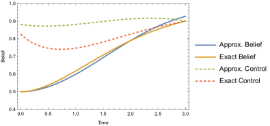
Figure 5: Belief evolution and control for the $\theta^{\prime}$-control formulation of Eq. 13. The plot shows solution curves for the exact formulation of the control Hamiltonian as well as the second-order approximation in belief coordinates $q$. The boundary values correspond to $q_{0}=0.5$, $p_{0}=0$ and $q_{f}=0.9$ with $\alpha=0.5,\beta=10,k=1$ and time horizon $T=3$.

While proximity to the geometric boundary drives stiffness in the control problem, this can be ameliorated to some extent by choosing a longer time horizon $T$. We can very roughly approximate a lower bound for an acceptable time horizon by solving the approximate control problem with the maximum (minimum) possible control input $\theta^{\prime}=\pi$ ($\theta^{\prime}=0$), to estimate the shortest horizon over which the desired belief target can be met without “wrapping” the control. While this lower bound doesn’t have a clean analytic formula, it is straightforward to compute numerically. Using the parameter values above the minimum time horizon to avoid wrapping is $T\approx 1.9$. Numerical experimentation indicates that reasonable control solutions can be found for $T>2.2$, below which both the exact system and the forward simulation of the approximate control system become stiff. Notably as $T$ approaches this threshold the approximate control curve gets closer to the boundaries of the geometry, and the approximation breaks down.

As an alternative to controlling the belief distribution by changing $\theta^{\prime}$, we can instead fix $\theta^{\prime}=\theta_{f}$ to be the desired belief and use the spring constant $k$ as the control parameter. We use the same objective function as Eq. 13 with the quadratic cost $C=\beta k^{2}$. We use this cost for both the exact dynamics, given by $H$, and approximate dynamics, given by $H_{0}$. The resulting $k$-control problems do not appear to have a simple closed-form solution. However, the approximate control problem is again a LQC problem and both formulations are much better behaved numerically than the $\theta^{\prime}$-control formulation. This is because the control parameter $k$ does not lie on the information manifold and is not as strongly impacted by the manifold curvature.

As an example, consider the same control problem as above except with $\theta^{\prime}=3\arccos\sqrt{0.9}$ and $T=1$. As before, we compute both the solution to the full control Hamiltonian as well as the approximate control Hamiltonian. For the approximate solution we again recompute the forward problem using the exact dynamics. The results are shown in Fig. 6. Again the second-order approximation provides reasonable control of the full system, although the approximate solution underestimates the response of the belief to the control variable for the same reasons as the $\theta^{\prime}$-control case. The approximate solution produces a final belief of $q_{f}=0.94$, instead of the intended target $q_{f}=0.9$.

Notably the time horizon for this formulation of the problem is smaller than the minimum threshold estimated for the $\theta^{\prime}$-control formulation. Since $k$ is not bounded by the information geometry there is no corresponding threshold in the $k$-control case and the numerical problem remains tractable down to $T\approx 0.1$.

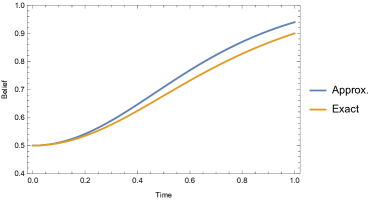
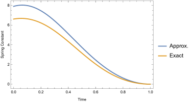
Figure 6: Belief evolution (top) and control (bottom) for the $k$-control formulation of Eq. 13. The plots show solution curves for the exact formulation of the control Hamiltonian as well as the second-order approximation in belief coordinates $q$. The boundary values correspond to $q_{0}=0.5$, $p_{0}=0$ and $q_{f}=0.9$ with $\alpha=0.5,\beta=10,\theta^{\prime}=2\arccos\sqrt{0.9}$ and time horizon $T=1$.

While a more thorough analysis of this information control problem, including joint $(k,\theta^{\prime})$-control, is outside the scope of this letter, this initial analysis indicates that the spring constant (i.e., social pressure) is a more robust control parameter than the observed belief. At a high level this is because the spring constant produces information potentials which scale linearly, while the observed belief can only achieve large potentials by interacting with the highly curved portions of the manifold boundary. Additionally, the simpler second-order approximation to the control problem, which utilizes traditional spring potentials and is a LQC problem, can produce effective control solutions, particularly in regions of high entropy.

In this letter, we introduced a model of belief combining Friston’s minimum energy principle and information geometry, making use of the Bayesian brain hypothesis. Using a Bernoulli distribution as a model of an agent’s belief about a bivalent topic (e.g., humans cause climate change), we showed how to recover a variant of DeGroot opinion dynamics via a classical Lagrangian. We further showed conditions under which opinion converges or comes to consensus through the use of a dissipative Lagrangian. In studying the nonlinear dynamics for two agents arising from the non-dissipative form of the Lagrangian, we showed that the corresponding Hamiltonian was a perturbation of a well-known integrable Hamiltonian. Despite the fact that the KAM theorem does not apply in this case, we illustrated symplectic flow near the fixed points and used Wolf’s algorithm to numerically prove the existence of chaotic behavior in trajectories near the boundary.

In studying the control problem arising from these dynamics, we identified interesting facts about the problem of persuasion. We found that manipulating peer pressure with a fixed (preferred) belief state is a more stable approach to altering an agent’s belief than providing a slowly changing belief state that approaches a target. These results may have real-world implications. Prior research shows that peer-pressure is a powerful motivator for inducing cooperation [70], especially (for example) in climate change beliefs and actions [71, 72]. Moreover, while information innoculation appears to be the most effective counter-misinformation strategy, research supports the hypothesis that “nudging” (through social pressure) provides a potentially useful way to counter-act misinformation as opposed to “debunking”, which has been shown to be less effective [73]. The mathematical results presented in this paper provide the first potential explanation for these empirical observations using a biophysical model. As such, further research into model generalizations may provide additional insights into persuasion and misinformation management.

References

- Friston et al. [2006] K. Friston, J. Kilner, and L. Harrison, A free energy principle for the brain, Journal of physiology-Paris 100, 70 (2006).
- Friston [2009] K. Friston, The free-energy principle: a rough guide to the brain?, Trends in cognitive sciences 13, 293 (2009).
- Friston [2010] K. Friston, The free-energy principle: a unified brain theory?, Nature reviews neuroscience 11, 127 (2010).
- Kiebel and Friston [2011] S. J. Kiebel and K. J. Friston, Free energy and dendritic self-organization, Frontiers in systems neuroscience 5, 80 (2011).
- Limanowski and Blankenburg [2013] J. Limanowski and F. Blankenburg, Minimal self-models and the free energy principle, Frontiers in human neuroscience 7, 547 (2013).
- Kwisthout and van Rooij [2015] J. Kwisthout and I. van Rooij, Free energy minimization and information gain: The devil is in the details, Cognitive neuroscience 6, 216 (2015).
- Buckley et al. [2017] C. L. Buckley, C. S. Kim, S. McGregor, and A. K. Seth, The free energy principle for action and perception: A mathematical review, Journal of Mathematical Psychology 81, 55 (2017).
- Bruineberg et al. [2018] J. Bruineberg, J. Kiverstein, and E. Rietveld, The anticipating brain is not a scientist: the free-energy principle from an ecological-enactive perspective, Synthese 195, 2417 (2018).
- Ramstead et al. [2018] M. J. D. Ramstead, P. B. Badcock, and K. J. Friston, Answering schrödinger’s question: A free-energy formulation, Physics of life reviews 24, 1 (2018).
- Cieri et al. [2021] F. Cieri, X. Zhuang, J. Z. Caldwell, and D. Cordes, Brain entropy during aging through a free energy principle approach, Frontiers in Human Neuroscience 15, 647513 (2021).
- Aguilera et al. [2022] M. Aguilera, B. Millidge, A. Tschantz, and C. L. Buckley, How particular is the physics of the free energy principle?, Physics of Life Reviews 40, 24 (2022).
- Friston et al. [2023] K. Friston, L. Da Costa, N. Sajid, C. Heins, K. Ueltzhöffer, G. A. Pavliotis, and T. Parr, The free energy principle made simpler but not too simple, Physics Reports 1024, 1 (2023).
- Karl [2012] F. Karl, A free energy principle for biological systems, Entropy 14, 2100 (2012).
- Mazzaglia et al. [2022] P. Mazzaglia, T. Verbelen, O. Çatal, and B. Dhoedt, The free energy principle for perception and action: A deep learning perspective, Entropy 24, 301 (2022).
- Heins et al. [2024] C. Heins, B. Millidge, L. Da Costa, R. P. Mann, K. J. Friston, and I. D. Couzin, Collective behavior from surprise minimization, Proceedings of the National Academy of Sciences 121, e2320239121 (2024).
- Landauer [1961] R. Landauer, Irreversibility and heat generation in the computing process, IBM journal of research and development 5, 183 (1961).
- Plenio and Vitelli [2001] M. B. Plenio and V. Vitelli, The physics of forgetting: Landauer’s erasure principle and information theory, Contemporary physics 42, 25 (2001).
- Bennett [2003] C. H. Bennett, Notes on landauer’s principle, reversible computation, and maxwell’s demon, Studies In History and Philosophy of Science Part B: Studies In History and Philosophy of Modern Physics 34, 501 (2003).
- Bordel [2011] S. Bordel, Non-equilibrium statistical mechanics: partition functions and steepest entropy increase, Journal of Statistical Mechanics: Theory and Experiment 2011, P05013 (2011).
- Still et al. [2012] S. Still, D. A. Sivak, A. J. Bell, and G. E. Crooks, Thermodynamics of prediction, Physical review letters 109, 120604 (2012).
- Sivak and Crooks [2012] D. A. Sivak and G. E. Crooks, Thermodynamic metrics and optimal paths, Physical review letters 108, 190602 (2012).
- Kim et al. [2016] E.-j. Kim, U. Lee, J. Heseltine, and R. Hollerbach, Geometric structure and geodesic in a solvable model of nonequilibrium process, Physical Review E 93, 062127 (2016).
- Feng and Crooks [2009] E. H. Feng and G. E. Crooks, Far-from-equilibrium measurements of thermodynamic length, Physical review E 79, 012104 (2009).
- Kim and Hollerbach [2017] E.-j. Kim and R. Hollerbach, Geometric structure and information change in phase transitions, Physical Review E 95, 062107 (2017).
- Kim [2021] E.-j. Kim, Information geometry and non-equilibrium thermodynamic relations in the over-damped stochastic processes, Journal of Statistical Mechanics: Theory and Experiment 2021, 093406 (2021).
- Gomez et al. [2020] I. S. Gomez, M. Portesi, and E. P. Borges, Universality classes for the fisher metric derived from relative group entropy, Physica A: Statistical Mechanics and its Applications 547, 123827 (2020).
- Nicholson et al. [2020] S. B. Nicholson, L. P. García-Pintos, A. del Campo, and J. R. Green, Time–information uncertainty relations in thermodynamics, Nature Physics 16, 1211 (2020).
- Dandekar et al. [2013] P. Dandekar, A. Goel, and D. T. Lee, Biased assimilation, homophily, and the dynamics of polarization, Proceedings of the National Academy of Sciences 110, 5791 (2013).
- Semonsen et al. [2018] J. Semonsen, C. Griffin, A. Squicciarini, and S. Rajtmajer, Opinion dynamics in the presence of increasing agreement pressure, IEEE transactions on cybernetics 49, 1270 (2018).
- Griffin et al. [2022a] C. Griffin, A. Squicciarini, and F. Jia, Consensus in complex networks with noisy agents and peer pressure, Physica A: Statistical Mechanics and its Applications 608, 128263 (2022a).
- McDonald [2015] K. T. McDonald, A damped oscillator as a hamiltonian system, Joseph Henry Laboratories, Princeton University (2015).
- Bersani and Caressa [2021] A. M. Bersani and P. Caressa, Lagrangian descriptions of dissipative systems: a review, Mathematics and Mechanics of Solids 26, 785 (2021).
- DeGroot [1974] M. H. DeGroot, Reaching a consensus, J. American Stat. Association 69, 118 (1974).
- Krause [2000] U. Krause, A discrete nonlinear and non-autonomous model of consensus formation, in In Communications in Difference Equations, edited by Gordon and Breach (2000) pp. 227– 236.
- Hegselmann and Krause [2002] R. Hegselmann and U. Krause, Opinion dynamics and bounded confidence: Models, analysis and simulation, J. Artificial Soc. Social Simul. 5 (2002).
- Ben-Naim [2005] E. Ben-Naim, Opinion dynamics: Rise and fall of political parties, Europhys. Lett. 69, 671 (2005).
- Weisbuch et al. [2005] G. Weisbuch, G. Deffuant, and F. Amblard, Persuasion dynamics, Physica A 353 (2005).
- Toscani [2006] G. Toscani, Kinetic models of opinion formation, Commun. Math. Sci. 4, 481 (2006).
- Weisbuch [2006] G. Weisbuch, Social opinion dynamics, in Econophysics and Sociophysics: Trends and Perspectives, edited by B. K. Chakrabarti, A. Chakrabarti, and A. Chatterjee (Wiley, 2006) pp. 67–94.
- Lorenz [2007] J. Lorenz, Continuous opinion dynamics of multidimensional allocation problems under bounded confidence. a survey, Internat. J. Modern Phys. C 18, 1819 (2007).
- Blondel et al. [2009] V. D. Blondel, J. M. Hendrickx, and J. N. Tsitsiklis, On krause’s multi-agent consensus model with state-dependent connectivity, IEEE Transactions on Automatic Control 54, 2586 (2009).
- Castellano et al. [2009] C. Castellano, S. Fortunato, and V. Loreto, Statistical physics of social dynamics, Reviews of modern physics 81, 591 (2009).
- Kurz and Rambau [2011] S. Kurz and J. Rambau, On the hegselmann-krause conjecture in opinion dynamics, J. Difference Equ. Appl. 17, 859 (2011).
- Duering et al. [2012] B. Duering, P. Markowich, J. F. Pietschmann, and M. T. Wolfram, Boltzmann and Fokker-Planck equations modelling opinion formation in the presence of strong leaders, Proc. R. Soc. Lond. Ser. A 465 (2012).
- Canuto et al. [2012] C. Canuto, F. Fagnani, and P. Tilli, An eulerian approach to the analysis of krause’s consensus models, SIAM J. Contr. and Opt. , 243 (2012).
- Jabin and Motsch [2014] P.-E. Jabin and S. Motsch, Clustering and asymptotic behavior in opinion formation, Journal of Differential Equations 257, 4165 (2014).
- Shang et al. [2021] L. Shang, M. Zhao, J. Ai, and Z. Su, Opinion evolution in the sznajd model on interdependent chains, Physica A: Statistical Mechanics and its Applications 565, 125558 (2021).
- Glass and Glass [2021] C. A. Glass and D. H. Glass, Opinion dynamics of social learning with a conflicting source, Physica A: Statistical Mechanics and its Applications 563, 125480 (2021).
- Centola and Baronchelli [2015] D. Centola and A. Baronchelli, Flocks, herds, and schools: A quantitative theory of flocking, Proceedings of the National Academy of Sciences 112, 1989 (2015).
- Toner and Tu [1998] J. Toner and Y. Tu, Flocks, herds, and schools: A quantitative theory of flocking, Physical Review E 58, 4828 (1998).
- Cucker and Smale [2007] F. Cucker and S. Smale, Emergent behavior in flocks, IEEE Transactions on Automatic Control 52, 852 (2007).
- Edelstein-Keshet [2001] L. Edelstein-Keshet, Mathematical models of swarming and social aggregation, in Proc. 2001 International Symposium on Nonlinear Theory and Its Applications (NOLTA 2001) (Miyagi, Japan, 2001).
- Li [2008] W. Li, Stability analysis of swarms with general topology, IEEE Trans. Systems, Man and Cybernetics, Part B 38, 1084 (2008).
- Li and Xiao [2010] X. Li and J. Xiao, Swarming in homogeneous environments: A social interaction based framework, J. Theoret. Biol. 264, 747 (2010).
- Degond and Motsch [2011] P. Degond and S. Motsch, A macroscopic model for a system of swarming agents using curvature control, J. Stat. Phys. 143 (2011).
- Motsch and Tadmor [2014] S. Motsch and E. Tadmor, Heterophilious Dynamics Enhances Consensus, SIAM Review 56, 577 (2014).
- Nielsen [2018] F. Nielsen, An elementary introduction to information geometry, CoRR abs/1808.08271 (2018), 1808.08271 .
- Griffin [2021] C. Griffin, A comment on and correction to: Opinion dynamics in the presence of increasing agreement pressure, IEEE Transactions on Cybernetics (2021).
- Gavrilets et al. [2016] S. Gavrilets, J. Auerbach, and M. Van Vugt, Convergence to consensus in heterogeneous groups and the emergence of informal leadership, Scientific Reports 6, 29704 (2016).
- Fink et al. [2002] E. L. Fink, S. A. Kaplowitz, and S. M. Hubbard, Oscillation in beliefs and decisions, The Persuasion Handbook: Developments in Theory and Practice. Thousand Oaks, CA: Sage Publications , 17 (2002).
- Kaplowitz et al. [1996] S. Kaplowitz, E. Fink, J. Watt, and C. Van Lear, Cybernetics of attitudes and decisions, Dynamic patterns in communication processes , 277 (1996).
- Zaslavsky [1992] G. M. Zaslavsky, Weak chaos and quasi-regular patterns, 1 (Cambridge University Press, 1992).
- Wolf et al. [1985] A. Wolf, J. B. Swift, H. L. Swinney, and J. A. Vastano, Determining lyapunov exponents from a time series, Physica D: nonlinear phenomena 16, 285 (1985).
- Griffin et al. [2022b] C. Griffin, J. Semonsen, and A. Belmonte, Generalized hamiltonian dynamics and chaos in evolutionary games on networks, Physica A: Statistical Mechanics and its Applications 597, 127281 (2022b).
- Arnol’d [2013] V. I. Arnol’d, Mathematical methods of classical mechanics, Vol. 60 (Springer Science & Business Media, 2013).
- Goehle and Griffin [2024] G. Goehle and C. Griffin, Free entropy minimizing persuasion in a predictor-corrector dynamic, Physica A: Statistical Mechanics and its Applications , 129819 (2024).
- Johnson and Gibson [1963] C. Johnson and J. Gibson, Singular solutions in problems of optimal control, IEEE Transactions on Automatic Control 8, 4 (1963).
- Kirk [2004] D. E. Kirk, Optimal control theory: an introduction (Courier Corporation, 2004).
- Sachkov [2022] Y. Sachkov, Optimal control problem, in Introduction to Geometric Control (Springer International Publishing, Cham, 2022) pp. 47–79.
- Mani et al. [2013] A. Mani, I. Rahwan, and A. Pentland, Inducing peer pressure to promote cooperation, Scientific reports 3, 1735 (2013).
- Delina and Delina [2019] L. L. Delina and L. L. Delina, Triggering communal peer pressure: Spreading a shared understanding of demands, Emancipatory Climate Actions: Strategies from histories , 71 (2019).
- Stevenson et al. [2019] K. T. Stevenson, M. N. Peterson, and H. D. Bondell, The influence of personal beliefs, friends, and family in building climate change concern among adolescents, Environmental Education Research 25, 832 (2019).
- Roozenbeek et al. [2023] J. Roozenbeek, E. Culloty, and J. Suiter, Countering misinformation, European Psychologist (2023).