A quantum mechanical evaluation
of the intermediate scattering function
Abstract
The intermediate scattering function is interpreted as a correlation function of thermal wave packets of the scattering centers perturbed by the scattering particles at different times. A proof of concept is given at the example of ballistic moving centers. The ensuing numerical method is then illustrated at the example of CO adsorbed on Cu(100).
The van Hove formula van Hove (1954) for the intermediate scattering function (ISF) has been used for more than half a century in the investigation of the dynamics of condensed matter (Vineyard, 1957; Schofield, 1960; Chudley and Elliot, 1961; Gunn and Warner, 1984; Dattagupta et al., 1989; Kob and Andersen, 1995; Jardine et al., 2009a; Townsend and Chin, 2019, and references cited therein, this list being rather incomplete). It is given by the expression
| (1) |
Here is the Hamiltonian of the scattering centers at positions and , is the wave vector pertaining to the change of momentum during the scattering and is a time; is the thermal density operator, where is the temperature of the scattering system, and is the canonical partition function; is the Planck constant divided by and is the Boltzmann constant. This function is also known as the space Fourier transformation of the space-time pair correlation function.
More recently, the ISF was also evoked in the context of helium scattering experiments to determine diffusion coefficients of adsorbed atoms and molecules on surfaces Jardine et al. (2009a). So far, in these investigations, the ISF is mainly evaluated from molecular dynamics simulations following the laws of classical mechanics, i.e. by interpreting the factors in terms of the classical mechanical trajectories .
As was already noted by van Hove himself van Hove (1954), cannot be cast into the form with some time dependent operator in the Heisenberg representation. The ISF is thus not a conventional time dependent quantum mechanical observable. Rather, it is a quantum correlation function Kubo et al. (1992). While the classical evaluation of the ISF relates to the correlation of particles at positions and under thermal conditions, its pure quantum mechanical evaluation is not obviously connected to a time correlation of positions, as the particles’ density is constant and delocalized in a thermal quantum mechanical state. Townsend and Chin derived an analytical quantum dynamical expression for the ISF on the basis of tight binding model Hamiltonians and the Baker-Campbell-Hausdorff disentangling theorem Townsend and Chin (2019), providing theoretical evidence for long-range coherent tunneling in helium-3 scattering experiments.
In this letter we demonstrate that the ISF can be interpreted as the correlation between two typical members of the thermal ensemble: the first one is a thermal wave packet that is perturbed by the interaction with the scattering particle beam at time ; the second one is a thermal wave packet perturbed at time . A proof of principle is given at the example of the ballistic particle, for which the ISF is known analytically van Hove (1954). This interpretation allows us to evaluate the ISF from the quantum dynamical evolution of the scattering centers in a general way. In order to illustrate the potential applicability of the ensuing method, the ISF is then calculated within a model study of a CO particle moving on a Cu(100) substrate.
Following Tolman Tolman (1938), the thermal density operator may be considered to be a statistically averaged operator , where . The states constitute a stochastic ensemble of time dependent, pure states characterized by random variables and called stochastic thermal wave packets:
| (2) |
Here, it is assumed that the system of scattering particles has a discrete spectrum with system’s eigenstates : . Note that the statistical average annihilates the time dependency of , so that one may as well write .
For simplicity, and without lack of generality, consider in the following a system composed of a single particle. Because taking the ensemble average and the trace commute, we may set
| (3) |
where
| (4) | |||||
Note that . Let now
| (5) |
be a thermal state that is “kicked” by the scattering operator at time zero. Indeed, the state resulting from the action of the scattering operator on a momentum eigenstate with yields just the shifted momentum eigenstate .
Its time evolution is then . Similarly, let
| (6) |
be the same thermal state that has evolved with time and is then “kicked” by the same scattering operator.
We may then write
| (7) | |||||
Individual statistically tagged ISF functions can thus be understood as yielding the correlation between a kicked and then time evolved thermal wave packet and the same time evolved and then kicked thermal wave packet . The latter represent two states of the scattering centers that result from their interaction with the helium atoms at different times. The observable ISF is then obtained as the ensemble average over these correlations in Eq. (3). Such correlations sample the degree of order in the statistical ensemble. At finite temperature, they should decay in time as the delay between the two events, i.e. the “kicks”, increases. This is precisely the observed behavior for the experimental ISF, although experimentally, other processes might also contribute to the decay.
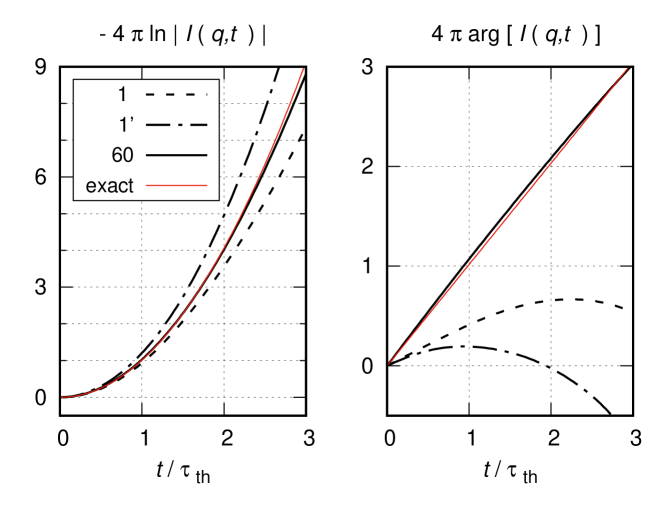
As a proof of concept, we evaluate Eq. (7) numerically for a free particle of mass moving at constant temperature. In this case the ISF is known analytically van Hove (1954):
| (8) |
where is a complex valued mean square displacement (MSD). Note that is the classical mechanical result for the MSD of the ballistic particle. In the natural units and , the MSD becomes , so that
| (9) |
Figure 1 shows the numerical evaluation of these functions (black continuous and dotted lines) and the exact values (red lines) for (). Here, the Schrödinger equation is solved for the free particle Hamiltonian in a box of length on a grid of 800 points. For each stochastic sample, calculations are converged to within relative precision in length and time over the time interval presented in the figure. Numerical results are surprisingly smooth. Yet, single stochastic samples differ significantly from the exact values as time evolves. Only after some substantial averaging, 60 in the example, one starts to achieve acceptable agreement between the numerical and the analytical results. Interestingly, the phase of the ISF needs somewhat more samplings to converge than its amplitude.
Evaluating Eqs. (7) and then (3) is a method to determine the ISF from first principle calculations. As an illustration, we evaluate these formulae for a simplified, albeit realistic model of CO moving on Cu(100). This system was investigated in helium-3 experiments Alexandrowicz et al. (2004); Jardine et al. (2009b). Here, however, we are not attempting to calculate accurately experimental rates. Rather, we wish to show that the evaluation of Eq. (7) leads to a qualitative temporal behavior of the ISF that is also found in experiments at realistic time scales.
We consider a one-dimensional model of the system along the crystallographic direction. The periodic model potential energy function was developed in refs. 14 and 15 from first principle calculations. The model potential was also used in previous related work Zanuttini et al. (2018); Marquardt (2022), were defining parameters are given. As reported in ref. 15, the barrier energy for jumps between stable CO adsorption sites is 33.5 meV and includes a significant variation of the zero point energy. The potential accommodates 13 bands of hindered translational levels up to this barrier, which correspond classically to confined vibrational motion within an adsorption well. The first excited band lies about 1.8 meV above the ground level. With increasing energy, bands become broader due to tunneling to neighboring wells Zanuttini et al. (2018). At 190 K, for instance, the higher most band below the barrier still has a relative population of about 15% with respect to the ground level. The thermal wave packet contains thus a large portion of energy eigenstates below the barrier, but also states above it. In the numerical evaluation, a grid of 80 elementary cells with individual cell length of , the Cu(100) lattice constant, and 50 points per cell was used, which yields converged calculations. Ensemble averages are converged with 20 samples.
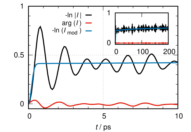
Initially, (black line), followed by piece-wise periodic oscillations with smaller amplitudes around a median, slowly ascending line (drawn in blue color) and periods of about 1.5 ps. The phase of the ISF (red line) oscillates in a similar irregular way around zero. Note that, , the mean square displacement (MSD) Vineyard (1957); Schofield (1960); Chudley and Elliot (1961). A typical behavior found in early experimental work on neutron scattering is explained by the jump model of Chudley and Elliott, which “predicts a width like the Debye model with some slight increase at large ” Chudley and Elliot (1961). This behavior of the ISF is quite generally also found in the spin echo polarization decay and is featured by the black line in Figure 2.
The MSD of a harmonic oscillator behaves as also quantum mechanically Marquardt (2022) which explains the initial quadratic increase of the black line. The approximate period of 1.5 ps matches roughly from the fundamental transition energy . The potential is highly anharmonic, though, which explains the irregular periodic behavior and the imperfect matching of periods. Quite generally, the quantum dynamics of anharmonic vibrations becomes rapidly irregular Marquardt and Quack (1989). This apparent lack of coherence is even more pronounced for strongly anharmonically coupled vibrations in high dimensional systems where survival probabilities decay approximately exponentially and oscillations are “coherently” damped Marquardt and Quack (1991). In the context of apparently statistical time-dependent quantum dynamics we should mention the famous Bixon-Jortner model for radiationless transitions Bixon and Jortner (1968), see also ref. 21 and references cited therein.
In the present, one-dimensional study, oscillations persist for longer times, as can be seen from the inset. The blue median line around which the ISF oscillates results from a model, smooth representation of the ISF. In the analysis of the experimental work, the ISF is often modeled by a double-exponential decaying function Jardine et al. (2009b) which smooths down the oscillations that are observed in the initial phase of the ISF evolution. Here, we use the model function
| (10) |
This model ensures that for short times, which is a reasonable assumption to make, as for short times the ballistic character of the motion prevails, whether the particle is moving freely or in a harmonic potential well. Adjustment of to the data defining the black line up to 200 ps yields (uncertainties are 68% confidence intervals) which define the blue line in Figure 2. They hold for . To test their reliability, the ISF was calculated to up to 400 ps, while model and parameters keep on describing well the median of the extended function. We note that each realization from Eq. (7) is the result of a coherent quantum dynamical evolution of a thermal wave packet. The stochastic nature of the latter, which stems from the random phases in Eq. (2), induces some fluctuation between individual realizations. The ISF depicted in Figure 2 was obtained from averaging 20 individual stochastic realizations of the ISF, Eq. (3).
The time Fourier transformation of the ISF yields the dynamical structure factor (DSF) van Hove (1954). The first exponential in Eq. (10) gives a broad Gaussian, the second a much sharper Lorentzian DSF. In the analysis of the spin-echo data, one usually considers the quasielastic broadening of the sharper part of the DSF as indicative of intercell diffusion Jardine et al. (2004). The corresponding rate of the ISF is called dephasing rate in spin-echo experiments Jardine et al. (2009b). It is interesting to compare the value of with dephasing rates.
The time scale of the slow decay rate is indeed comparable with the dephasing rate from figure 7 of ref. 13 for in the direction. This is nearly 3/4 of . Before drawing any further conclusion from this comparison with respect to the quality of the treatment and, in particular, to the accuracy of the model used, one has to bear in mind the major approximations made to obtain Figure 2. Caveats of the present model are the one-dimensional treatment and the neglect of dissipation during the dynamics. Furthermore, the potential energy function model might be incorrect, despite its origin from first principle calculations. The rough agreement between and could just be a fortuitous compensation of errors.
Figure 2 shows nevertheless that Eq. (7) is tenable to pick up a temporal behavior of the ISF that is found experimentally at comparable time scales. Intrinsic quantum dynamical properties of the motion such as the non-local distribution of thermal probability densities, irregular interference effects between waves pertaining to individual eigenstates of the system in the thermal wave packet and, last but not least, tunneling quite naturally lead to a roughly exponential decay of the ISF in the long time limit that is comparable with experimental findings despite the neglect of explicit dissipative effects in the quantum dynamics. To the best of our knowledge, such a behavior has so far been exclusively rationalized in terms of dissipative dynamics.
The present theoretical treatment can be extended in order to include the multidimensional character of the motion as well as possible channels of dissipation during the dynamics Mandal et al. (2022a, b). Dissipation has been considered insofar as the thermal wave packet, Eq. (2), is the result of friction and its random phases mirror the resulting fluctuations. Dissipation is a continuous random process, however, and the time evolution of the thermal wave packet in Eq. (2) lacks the ongoing influence of the latter. For CO/Cu(100), friction is expected to become relevant in time intervals beyond 8 ps Alexandrowicz et al. (2004); Jardine et al. (2004). One could therefore expect the ISF depicted in the main part of Figure 2 to be essentially invariant in the presence of friction. For the inset up to 200 fs and beyond we presently cannot foresee its effect on the ISF in Eq. (7). One should expect that friction does not alter the absolute values of the coefficients in the thermal wave packets; very likely, friction could merely lead to a random reshuffling of their phases at random times. In the analysis of the experimental data, friction is partially responsible for the vibrational dephasing and the consequent reduction of the oscillatory behavior of the ISF Jardine et al. (2004). We note that the latter might as well result from “coherent” damping in multidimensional vibrational or vibronic dynamics Marquardt and Quack (1991, 2020).
Beyond being a rather straightforward method to evaluate the ISF within the framework of quantum mechanics, Eq. (7) is in the first place a novel interpretation of this quantity as a quantum time correlation function between two states, namely a perturbed (kicked) then time evolved and a time evolved then perturbed (kicked) thermal wave packet. These are states of the scattering centers at thermal conditions having interacted with the scattering beam at different times. Individually, thermal wave packets are pure states and only ensemble averages are reasonably comparable with experimental findings obtained under these conditions. Further work to explore the and -dependence of the ISF is in progress. It will in particular be aimed at including friction and higher dimensions in the dynamical calculations to ensure the predictability and accuracy of the method.
Acknowledgements.
This work benefits from a grant received from the French Agence Nationale de la Recherche (ANR) under project QDDA. We wish to express our gratitude to Hans-Dieter Meyer and all the developers of the Heidelberg MCTDH program package, which was used for the numerical work presented here.References
- van Hove (1954) L. van Hove, Phys. Rev. 95, 249 (1954).
- Vineyard (1957) G. H. Vineyard, J. Phys. Chem. Solids 3, 121 (1957).
- Schofield (1960) P. Schofield, Phys. Rev. Lett. 4, 239 (1960).
- Chudley and Elliot (1961) C. T. Chudley and R. J. Elliot, Proc. Phys. Soc. 77, 353 (1961).
- Gunn and Warner (1984) J. M. F. Gunn and M. Warner, Z. Phys. B Condensed Matter 56, 13 (1984).
- Dattagupta et al. (1989) S. Dattagupta, H. Grabert, and R. Jung, Journal of Physics: Condensed Matter 1, 1405 (1989).
- Kob and Andersen (1995) W. Kob and H. C. Andersen, Phys. Rev. E 51, 4626 (1995).
- Jardine et al. (2009a) A. P. Jardine, H. Hedgeland, G. Alexandrowicz, W. Allison, and J. Ellis, Prog. in Surf. Sci. 84, 323 (2009a).
- Townsend and Chin (2019) P. S. M. Townsend and A. W. Chin, Phys. Rev. A 99, 012112 (2019).
- Kubo et al. (1992) R. Kubo, M. Toda, and N. Hashitsume, Statistical Physics II, Nonequilibrium Statistical Mechanics, 2nd ed. (Springer, Heidelberg, 1992).
- Tolman (1938) R. C. Tolman, The principles of statistical mechanics (Oxford University Press, Oxford (UK), 1938).
- Alexandrowicz et al. (2004) G. Alexandrowicz, A. P. Jardine, P. Fouquet, S. Dworski, W. Allison, and J. Ellis, Phys. Rev. Lett. 93, 156103 (2004).
- Jardine et al. (2009b) A. P. Jardine, G. Alexandrowicz, H. Hedgeland, W. Allison, and J. Ellis, Phys. Chem. Chem. Phys. 11, 3355 (2009b).
- Marquardt et al. (2010) R. Marquardt, F. Cuvelier, R. A. Olsen, E. J. Baerends, J. C. Tremblay, and P. Saalfrank, J. Chem. Phys. 132, 074108 (2010).
- Firmino et al. (2015) T. Firmino, R. Marquardt, F. Gatti, D. Zanuttini, and W. Dong, in Frontiers in Quantum Methods and Applications in Chemistry and Physics: Selected and Edited Proceedings of QSCP-XVIII (Paraty, Brazil, December 2013), Progress in Theoretical Chemistry and Physics, edited by M. A. C. Nascimento (Springer, Berlin, 2015).
- Zanuttini et al. (2018) D. Zanuttini, F. Gatti, and R. Marquardt, Chem. Phys. 509, 3 (2018).
- Marquardt (2022) R. Marquardt, Phys. Chem. Chem. Phys. 24, 26519 (2022).
- Marquardt and Quack (1989) R. Marquardt and M. Quack, J. Chem. Phys. 90, 6320 (1989).
- Marquardt and Quack (1991) R. Marquardt and M. Quack, J. Chem. Phys. 95, 4854 (1991).
- Bixon and Jortner (1968) M. Bixon and J. Jortner, The Journal of Chemical Physics 48, 715 (1968).
- Marquardt and Quack (2020) R. Marquardt and M. Quack, eds., Molecular Spectroscopy and Quantum Dynamics (Elsevier, St. Louis (Missouri), USA, 2020).
- Jardine et al. (2004) A. P. Jardine, J. Ellis, and W. Allison, J. Chem. Phys. 120, 8724 (2004).
- Mandal et al. (2022a) S. Mandal, F. Gatti, O. Bindech, R. Marquardt, and J.-C. Tremblay, The Journal of Chemical Physics 156, 094109 (2022a).
- Mandal et al. (2022b) S. Mandal, F. Gatti, O. Bindech, R. Marquardt, and J. C. Tremblay, The Journal of Chemical Physics 157, 144105 (2022b).