Effect of Lyman-$\alpha$ Radiative Transfer on Intensity Mapping Power Spectra

Abstract

Clustering of Lyman-$\alpha$ (Ly$\alpha$) emitting galaxies (LAEs) is a useful probe of cosmology. However, Ly$\alpha$ radiative transfer (RT) effects, such as absorption, line shift, and line broadening, and their dependence on the large-scale density and velocity fields can modify the measured LAE clustering and line intensity mapping (LIM) statistics. We explore the effect of RT on the Ly$\alpha$ LIM power spectrum in two ways: using an analytic description based on linear approximations and using lognormal mocks. The qualitative effect of intergalactic Ly$\alpha$ absorption on the LIM auto- and cross-power spectrum is a scale-dependent, reduced effective bias, reduced mean intensity, and modified redshift-space distortions. The linear absorption model does not describe the results of the lognormal simulations well. The random line shift suppresses the redshift-space power spectrum similar to the Fingers-of-God effect. In cross-correlation of LAEs or Ly$\alpha$ intensity with a non-Ly$\alpha$ tracer, the Ly$\alpha$ line shift leads to a phase shift of the complex power spectrum, i.e. a cosine damping of the real part. Line broadening from RT suppresses the LIM power spectra in the same way as limited spectral resolution. We study the impact of Ly$\alpha$ RT effects on the Hobby-Eberly Telescope Dark Energy Experiment (HETDEX) LAE and LIM power spectra using lognormal mocks. We find that even small amounts of IGM absorption will significantly change the measured LAE auto-power spectrum and the LAE-intensity cross-power spectrum. Therefore, HETDEX will be able to constrain Ly$\alpha$ RT effects.

1 Introduction

The Lyman-$\alpha$ (Ly$\alpha$) emission line is an excellent tool for cosmology at high redshift (e.g.; Partridge & Peebles, 1967). Detected Ly$\alpha$-emitting galaxies (LAEs) are used to measure their clustering and constrain cosmological parameters (Ouchi et al., 2020; Gebhardt et al., 2021). Instead of detecting individual LAEs in deep observations with high resolution, one can also map the total Ly$\alpha$ intensity in noisy, low-resolution observations to constrain cosmological parameters, called line intensity mapping (LIM, e.g.; Bernal & Kovetz, 2022).

Neutral hydrogen has a large scattering cross-section around the Ly$\alpha$ line. The radiative transfer (RT) complicates the interpretation of measurements using Ly$\alpha$ emission. For example, using simulations, Zheng et al. (2011) find a strong correlation between the Ly$\alpha$ optical depth in the intergalactic medium (IGM) and the large-scale density and velocity structure. They predict that the anisotropic dependence of the observed fraction of LAEs suppresses line-of-sight (LOS) density fluctuations, makes the effective bias scale-dependent, and can even ‘invert’ the so-called Kaiser effect (Kaiser, 1987), the linear redshift-space distortions (RSD).

One can model the effect of IGM absorption on the LIM power spectra in various ways. Wyithe & Dijkstra (2011) (from now on WD11, ) and Greig et al. (2013) derive an analytic model for this effect for the power spectrum and bispectrum. The analytic absorption model for the power spectrum in the first part of WD11 is based on linear approximations for the dependence of the Ly$\alpha$ transmittance on the matter, ionization rate, and velocity distributions. While this explains the qualitative effect of IGM absorption on the power spectrum, the amplitude is determined by three free parameters: the mean optical depth $\tau_{0}$, the fraction of Ly$\alpha$ photons subject to IGM absorption $F_{\mathrm{abs}}$, and the smoothing kernel of the ionization rate with respect to the galaxy distribution. The linear approximations are also only valid when the matter overdensity $\delta_{\mathrm{m}}$, the ionization rate perturbations $\delta_{\Gamma}$, and the velocity gradient perturbations $\delta_{v}$ are small, which is not the case in the immediate environments of galaxies. WD11 also present a more detailed analytic model that is based on assumptions on the density profile, ionization rate, temperature, and gas velocities in the environment of the LAEs.

Using a cosmological hydrodynamical simulation and post-processing it with Ly$\alpha$ RT, such as Zheng et al. (2011), Behrens & Niemeyer (2013) and Behrens et al. (2018), may provide the most realistic estimate for the optical depth and the effect on the observed fluxes and the power spectrum if it accurately simulates the matter and velocity structure within and outside of the galaxy halos. However, the results of these simulations are dependent on the resolution: using an RT simulation with higher resolution, Behrens et al. (2018) find little correlation between the large-scale environment and the observed fraction of LAEs, while they reproduce the results of Zheng et al. (2011) when they degrade the resolution of the simulation.

Gurung-López et al. (2020) develop a semi-analytic model for Ly$\alpha$ RT in the interstellar medium (ISM) and IGM. They find that at low redshift ($z\in[2.2,3]$) the spatial distribution of LAEs is independent of IGM properties. However, at $z=5.7$, the LOS velocity and density gradients modify the clustering of LAEs on large scales in an isotropic fashion.

Another effect of the Ly$\alpha$ RT in the ISM and circumgalactic medium (CGM) is the broadening and the shift of the Ly$\alpha$ line, typically towards the red (e.g.; Nakajima et al., 2018). Byrohl et al. (2019) find in a cosmological RT simulation that this wavelength shift is independent of the large-scale velocities and show that the shift adds a Fingers-of-God-like damping to the LAE power spectrum.

Croft et al. (2016) observationally find a strong effect of RT on the cross-correlation of quasars with Ly$\alpha$ intensity. However, more recent studies are consistent with the absence of RT effects (Croft et al., 2018; Lin et al., 2022). More observations of LAE clustering or Ly$\alpha$ LIM are necessary to constrain RT effects. The Hobby-Eberly Telescope Dark Energy Experiment (HETDEX; Gebhardt et al., 2021) uses integral-field spectrographs to find $\simeq 10^{6}$ LAEs without target preselection in a $10.9\,\mathrm{Gpc}^{3}$ comoving volume. Its primary goal is to use LAE clustering statistics such as the power spectrum to constrain cosmological parameters, especially the dark energy equation of state (Shoji et al., 2009). The blind nature of HETDEX enables Ly$\alpha$ LIM studies that may also be affected by Ly$\alpha$ RT effects. We therefore explore these effects on LIM power spectra and estimate the sensitivity of a HETDEX-like survey to these effects.

In this paper, we explore the effect of Ly$\alpha$ absorption in the IGM and the line shift and broadening on the Ly$\alpha$ intensity auto- and cross-power spectra. We use lognormal simulations for the forecast. Simple is a fast simulation tool for self-consistently generating galaxy catalogs and intensity maps in redshift space given an input power spectrum and luminosity function (Lujan Niemeyer et al., 2023). It is based on a lognormal galaxy catalog generator (Agrawal et al., 2017), assigns luminosities, determines the detectability of each galaxy, and generates an intensity map. One can apply smoothing and a mask and add noise to make the mocks more realistic. Because the matter density and velocity fields are output by the lognormal galaxy simulations, one can self-consistently calculate the Ly$\alpha$ optical depth in each resolution element and attenuate the luminosities accordingly to simulate IGM absorption. Adding a random line shift and broadening is also straight-forward.

A drawback of hydrodynamic simulations and semi-analytic models is their computational cost, which makes it unfeasible to generate enough realizations to calculate a covariance matrix and make sensitivity forecasts. Because lognormal simulations are fast, it is possible to generate enough mocks to calculate the covariance matrix for the HETDEX survey and make predictions for its sensitivity to Ly$\alpha$ RT effects.

The rest of the paper is organized as follows. Section 2 builds on the model by WD11 to develop an analytic model for the IGM absorption for LIM auto- and cross-power spectra. Section 3 extends the work of Byrohl et al. (2019) on the effect of the line shift and broadening of the Ly$\alpha$ line to LIM power spectra. Section 4 describes the modifications to the Simple code to incorporate IGM absorption and a Ly$\alpha$ velocity shift and shows the effects on the different power spectra using the lognormal simulations. Section 5 analyses the sensitivity of a HETDEX-like experiment to these effects using Simple mocks for the HETDEX survey. Section 6 discusses the shortcomings of this approach. We conclude in Section 7.

We use the following Fourier convention:

$$\begin{split}\tilde{f}(\mathbf{k})&=\int\mathrm{d}^{3}\mathbf{x}f(\mathbf{x})e^{i\mathbf{k}\cdot\mathbf{x}}\,,\\ f(\mathbf{x})&=\int\frac{\mathrm{d}^{3}\mathbf{k}}{(2\pi)^{3}}\tilde{f}(\mathbf{k})e^{-i\mathbf{k}\cdot\mathbf{x}}\,,\end{split}$$ (1)

where the tilde denotes quantities in Fourier space. We refer to real space in contrast to redshift space, and to configuration space in contrast to Fourier space.

Throughout this paper, we assume a flat $\Lambda$ cold dark matter ($\Lambda$CDM) cosmology with $H_{0}=67.66\,\mathrm{km\,s^{-1}\,Mpc^{-1}}$, $\Omega_{\mathrm{b},0}h^{2}=0.022$, $\Omega_{\mathrm{m},0}h^{2}=0.142$, $\ln\left(10^{10}A_{s}\right)=3.094$, and $n_{s}=0.9645$.

2 Intergalactic Ly$\alpha$ Absorption

A Ly$\alpha$ photon escaping the CGM of a galaxy that is close enough to the Ly$\alpha$ line center can scatter off of neutral hydrogen on the IGM. Although the photon scatters out of the LOS, we refer to it as absorption in this work.

The optical depth for a photon with the initial frequency $\nu$ on its way from a galaxy’s virial radius to the observer is

$$\tau(\nu)=\int_{r_{\mathrm{vir}}}^{\infty}\mathrm{d}r\,n_{\mathrm{H}}(r)x_{\mathrm{HI}}(r)\sigma_{\alpha}\left[\nu\left(1+\frac{v_{z}(r)}{c}\right)\right],$$ (2)

where $n_{\mathrm{H}}(r)$ is the hydrogen number density, $x_{\mathrm{HI}}(r)$ is the neutral fraction of hydrogen, $v_{z}(r)$ is the LOS velocity of the gas at distance $r$ from the galaxy, where $v_{z}>0$ if it moves away from the observer, and $\sigma_{\alpha}(\nu)$ is the Ly$\alpha$ absorption cross-section at frequency $\nu$ (see, e.g.; WD11, ). Using $x_{\mathrm{HI}}=n_{\mathrm{H}}\alpha_{\mathrm{rec}}^{\mathrm{A}}/\Gamma$ at photoionization equilibrium, where $\Gamma$ is the photo-ionization rate and $\alpha_{\mathrm{rec}}^{\mathrm{A}}\approx 4.18\times 10^{-13}\,\mathrm{cm}^{3}\mathrm{s}^{-1}$ is the case-A recombination coefficient at temperature $T\approx 10^{4}\,\mathrm{K}$ (Burgess, 1965; Draine, 2011), we obtain

$$\tau(\nu)=\int_{r_{\mathrm{vir}}}^{\infty}\mathrm{d}r\,\frac{n_{\mathrm{H}}^{2}(r)\alpha_{\mathrm{rec}}^{\mathrm{A}}\sigma_{\alpha}\left[\nu\left(1+\frac{v_{z}(r)}{c}\right)\right]}{\Gamma(r)}.$$ (3)

Because the Ly$\alpha$ cross-section is within the integral, we can approximate it as a Dirac delta function

$$\begin{split}\sigma_{\alpha}(\nu)&\approx f_{\alpha}\pi\frac{e^{2}}{m_{e}c}\delta(\nu-\nu_{\alpha})\\ &=f_{\alpha}\pi r_{e}c\delta(\nu-\nu_{\alpha}),\end{split}$$ (4)

where $\nu_{\alpha}$ is the Ly$\alpha$ rest-frame frequency, $e$ is the electron charge, $m_{e}$ is the electron mass, $r_{e}=2.81\times 10^{-13}\,\mathrm{cm}$ is the classical electron radius defined by $\frac{e^{2}}{r_{e}}=m_{e}c^{2}$, and $f_{\alpha}=0.4167$ is the oscillator strength of the Ly$\alpha$ transition (e.g., WD11; Bartelmann, 2021). Inserting this in equation (3) and integrating yields

$$\tau_{\delta}=\frac{\left(c+v_{z}\right)n_{\mathrm{H}}^{2}\alpha_{\mathrm{rec}}^{\mathrm{A}}\sigma_{\alpha}^{\mathrm{tot}}}{\nu_{\mathrm{Ly\alpha}}\Gamma\left|\frac{\mathrm{d}v_{z}^{p}}{\mathrm{d}r}{{-H(z)}}\right|},$$ (5)

where $v_{z}^{p}$ denotes the peculiar velocity, so that $v_{z}=v_{z}^{p}-Hr$. Here, we used $\delta\left(g(r)\right)=\delta(r-r_{0})\left|g^{\prime}(r_{0})\right|^{-1}$, where $g^{\prime}$ denotes the derivative of $g$ with respect to $r$ and $g(r_{0})=0$. Specifically, $g(r)=\nu(r)-\nu_{\alpha}=\nu\left(1+v_{z}(r)/c\right)-\nu_{\alpha}$.

Because equation (2) only considers the absorption at distances larger than the virial radius, we summarize the RT within the galactic halo by using an effective absorption fraction. Like WD11, we introduce the fraction $F_{\mathrm{abs}}$ of Ly$\alpha$ photons subject to absorption as a free parameter, such that the fraction $1-F_{\mathrm{abs}}$ of photons travels freely. This is a simplified description of the line shape, where $1-F_{\mathrm{abs}}$ of the photons are redshifted outside of the high Ly$\alpha$ cross-section region from the RT within the ISM and CGM. The fraction $F_{\mathrm{abs}}$ of photons are close enough to or on the blue side of the Ly$\alpha$ line center to be subject to absorption. The total transmittance is given by integrating over the spectral flux density profile of the Ly$\alpha$ line $J(\nu)$, which becomes

$$\mathcal{T}=\frac{\int\mathrm{d}\nu\,J(\nu)e^{-\tau(\nu)}}{\int\mathrm{d}\nu\,J(\nu)}\approx 1-F_{\mathrm{abs}}+F_{\mathrm{abs}}e^{-\tau_{\delta}}.$$ (6)

2.1 Analytic Model for LIM Power Spectra

We modify the calculation of WD11 to derive a model for intergalactic Ly$\alpha$ absorption for the LIM power spectrum. Consider the Ly$\alpha$ intensity field as a biased tracer of the matter density with

$$\delta I(\mathbf{x})=I(\mathbf{x})-I_{0}(\mathbf{x})=I_{0}(\mathbf{x})b_{I}\delta_{\mathrm{m}},$$ (7)

where $b_{I}$ is the intensity bias, $\delta_{\mathrm{m}}=\rho(\mathbf{x})/\rho_{0}(\mathbf{x})-1$ is the matter density contrast, and $\rho(\mathbf{x})$ is the matter density. The subscript ₀ denotes the mean field over many realizations, for example the mean intensity or matter density as a function of redshift. We use brackets $\langle\cdot(\mathbf{x})\rangle$ to denote the same when it is more convenient. For simplicity, we consider a single redshift and therefore $I_{0}(\mathbf{x})=I_{0}=\mathrm{const.}$ Then the intensity power spectrum is

$$P_{II}(\mathbf{k})=\langle|\widetilde{\delta I}(\mathbf{k})|^{2}\rangle=b_{I}^{2}I_{0}^{2}P_{\mathrm{m}}(\mathbf{k}),$$ (8)

where $P_{\mathrm{m}}$ is the matter power spectrum and we neglected the discreteness of the intensity sources and therefore the shot noise contribution.

The intensity after IGM absorption can be approximated as

$$\begin{split}I^{\mathrm{abs}}(\mathbf{x})&=I^{\mathrm{abs}}_{0}\left[1+b_{I}\delta_{\mathrm{m}}(\mathbf{x})\right]\\ &+\left[\Gamma(\mathbf{x})-\Gamma_{0}\right]\left.\frac{\partial\mathcal{T}}{\partial\Gamma}\right|_{\mathcal{T}_{0},\Gamma_{0}}\left.\frac{\partial I^{\mathrm{abs}}}{\partial\mathcal{T}}\right|_{\mathcal{T}_{0}}\\ &+\left[\rho(\mathbf{x})-\rho_{0}\right]\left.\frac{\partial\mathcal{T}}{\partial\rho}\right|_{\mathcal{T}_{0},\rho_{0}}\left.\frac{\partial I^{\mathrm{abs}}}{\partial\mathcal{T}}\right|_{\mathcal{T}_{0}}\\ &+\left[\frac{\mathrm{d}v_{z}}{\mathrm{d}(ar_{\mathrm{com}})}-H\right]\left.\frac{\partial\mathcal{T}}{\partial\left(\frac{\mathrm{d}v_{z}}{\mathrm{d}(ar_{\mathrm{com}})}\right)}\right|_{\mathcal{T}_{0},H}\left.\frac{\partial I^{\mathrm{abs}}}{\partial\mathcal{T}}\right|_{\mathcal{T}_{0}}.\end{split}$$ (9)

We adopt the linear model of WD11 for the transmittance

$$\begin{split}\mathcal{T}(\delta_{\mathrm{m}},\delta_{\Gamma},\delta_{v})&=(1-F_{\mathrm{abs}})\\ &+F_{\mathrm{abs}}\exp\left\{-\tau_{0}\frac{1+c_{\gamma}\delta_{\mathrm{m}}}{1+\delta_{\Gamma}+\delta_{v}}\right\},\end{split}$$ (10)

where $\tau_{0}$ is the mean opacity in the IGM, $c_{\gamma}=(2.7-0.7\gamma)\simeq 1.72$ with the polytropic index $\gamma=1.4$ (Hui & Gnedin, 1997) denotes the dependence of the optical depth on dark matter density and $\delta_{\Gamma}=\frac{\Gamma}{\Gamma_{0}}-1$ is the ionization rate perturbation. The expression $\delta_{v}=\frac{\mathrm{d}v^{p}_{z}}{\mathrm{d}\left(ar_{\mathrm{com}}\right)}\frac{1}{H}$ represents the fluctuation in the LOS velocity. The dependence of the intensity on the transmittance is

$$\begin{split}\left.\frac{\partial I^{\mathrm{abs}}}{\partial\mathcal{T}}\right|_{\mathcal{T}_{0}}&=I_{0}=I_{0}^{\mathrm{abs}}\mathcal{T}_{0}^{-1}\\ &\approx I_{0}^{\mathrm{abs}}\left(1-F_{\mathrm{abs}}+F_{\mathrm{abs}}e^{-\tau_{0}}\right)^{-1}.\end{split}$$ (11)

We can rewrite equation (9):

$$\begin{split}\delta I^{\mathrm{abs}}(\mathbf{x})&=I^{\mathrm{abs}}(\mathbf{x})-I^{\mathrm{abs}}_{0}\\ &=I^{\mathrm{abs}}_{0}\left(b_{I}\delta_{\mathrm{m}}+\delta_{\mathrm{m}}C_{\rho}+\delta_{\Gamma}C_{\Gamma}+\delta_{v}C_{v}\right),\end{split}$$ (12)

where the constants $C_{x}$ are given by

$$\begin{split}C_{\Gamma}&=\left.\frac{\partial\mathcal{T}}{\partial\mathrm{log}\,\Gamma}\right|_{\mathcal{T}_{0},\Gamma_{0}}\left.\frac{\partial I^{\mathrm{abs}}}{\partial\mathcal{T}}\right|_{\mathcal{T}_{0}}(I_{0}^{\mathrm{abs}})^{-1}\\ C_{\rho}&=\left.\frac{\partial\mathcal{T}}{\partial\mathrm{log}\,\rho}\right|_{\mathcal{T}_{0},\rho_{0}}\left.\frac{\partial I^{\mathrm{abs}}}{\partial\mathcal{T}}\right|_{\mathcal{T}_{0}}(I_{0}^{\mathrm{abs}})^{-1}\\ C_{v}&=\left.\frac{\partial\mathcal{T}}{\partial\mathrm{log}\left(\mathrm{d}v_{z}/\mathrm{d}r_{\mathrm{com}}\right)}\right|_{\mathcal{T}_{0},H}\left.\frac{\partial I^{\mathrm{abs}}}{\partial\mathcal{T}}\right|_{\mathcal{T}_{0}}(I_{0}^{\mathrm{abs}})^{-1}.\end{split}$$ (13)

We find

$$C_{\Gamma}=C_{v}=\frac{F_{\mathrm{abs}}\tau_{0}e^{-\tau_{0}}}{1-F_{\mathrm{abs}}+F_{\mathrm{abs}}e^{-\tau_{0}}}=:C$$ (14)

and

$$C_{\rho}=-\frac{c_{\gamma}F_{\mathrm{abs}}\tau_{0}e^{-\tau_{0}}}{1-F_{\mathrm{abs}}+F_{\mathrm{abs}}e^{-\tau_{0}}}=-c_{\gamma}C.$$ (15)

The ionization rate fluctuations can be modeled by convolving the overdensity of ionizing sources with bias $b_{\mathrm{ion}}$ with a kernel $K_{\lambda}(k)=\mathrm{arctan}(k\lambda_{\mathrm{mfp}})/\left(k\lambda_{\mathrm{mfp}}\right)$, where $\lambda_{\mathrm{mfp}}$ is the mean free path of ionizing photons, so that

$$\tilde{\delta}_{\Gamma}(\mathbf{k})=b_{\mathrm{ion}}\tilde{\delta}_{\mathrm{m}}(\mathbf{k})K_{\lambda}(k).$$ (16)

The fluctuations of intensity introduced by observing in redshift space, denoted by the superscript ^s, are

$$\delta I^{\mathrm{s}}=\delta I-I_{0}\frac{\mathrm{d}v_{z}}{\mathrm{d}r_{\mathrm{com}}}\frac{1}{Ha}=\delta I-I_{0}\delta_{v}.$$ (17)

Relating the velocity gradient fluctuations to the density fluctuations as $\tilde{\delta}_{v}(\mathbf{k})=-f\mu^{2}\tilde{\delta}_{m}(\mathbf{k})$, where $f=\mathrm{d}\mathrm{ln}D/\mathrm{d}\mathrm{ln}a$ is the logarithmic growth factor, we can write

$$\begin{split}\widetilde{\delta I^{\mathrm{s}}_{\mathrm{abs}}}(\mathbf{k})&=I_{0}^{\mathrm{abs}}\tilde{\delta}_{\mathrm{m}}(\mathbf{k})\\ &\times\left[b_{I}+b_{\mathrm{ion}}K_{\lambda}(k)C_{\Gamma}+C_{\rho}+(1-C_{v})f\mu^{2}\right]\\ &=:I_{0}^{\mathrm{abs}}\tilde{\delta}_{\mathrm{m}}(\mathbf{k})D_{I}(\mathbf{k})=\mathcal{T}_{\mathrm{g}}I_{0}\tilde{\delta}_{\mathrm{m}}(\mathbf{k})D_{I}(\mathbf{k}).\end{split}$$ (18)

Here we assumed that the intrinsic luminosity of galaxies is uncorrelated with the local transmittance and $\mathcal{T}_{\mathrm{g}}=1-F_{\mathrm{abs}}+F_{\mathrm{abs}}{\int\mathrm{d}\mathbf{x}\,n(\mathbf{x})e^{-\tau(\mathbf{x})}}/{\int\mathrm{d}\mathbf{x}\,n(\mathbf{x})}$ is the effective mean transmittance around galaxies. The intensity auto-power spectrum is then given by

$$\begin{split}P_{II}(\mathbf{k})=\langle|\widetilde{\delta I^{\mathrm{s}}_{\mathrm{abs}}}(\mathbf{k})|^{2}\rangle=I_{0}^{2}\mathcal{T}_{\mathrm{g}}^{2}P_{\mathrm{m}}(k)D_{I}^{2}(\mathbf{k}).\end{split}$$ (19)

Taking a closer look at the intensity damping factor, we find

$$\begin{split}D_{I}&=b_{I}+b_{\mathrm{ion}}K_{\lambda}C-c_{\gamma}C+(1-C)f\mu^{2}\\ &=\left(b_{I}+b_{\mathrm{ion}}CK_{\lambda}-c_{\gamma}C\right)\\ &\times\left(1+\frac{f}{b_{I}}\mu^{2}\frac{b_{I}(1-C)}{b_{I}+b_{\mathrm{ion}}CK_{\lambda}-c_{\gamma}C}\right).\end{split}$$ (20)

The RSD-like effect of the IGM absorption is introduced because the RSD parameter $f/b_{I}$ is effectively multiplied by the factor ${(1-C)}/({1+CK_{\lambda}-c_{\gamma}C/b_{I}})$, assuming that $b_{I}=b_{\mathrm{ion}}$. This factor is smaller than one, i.e. the RSD is reduced, if $b_{I}>1.72$ on small scales, and $b_{I}>0.86$ on large scales.

Following WD11, the LAE overdensity in redshift space is

$$\begin{split}\widetilde{\delta}_{\mathrm{g_{\alpha}}}^{\mathrm{s}}&=\widetilde{\delta}_{\mathrm{m}}(\mathbf{k})\left[b_{\mathrm{g_{\alpha}}}+b_{\mathrm{ion}}C_{\Gamma}^{\mathrm{g_{\alpha}}}K_{\lambda}(k)+C_{\rho}^{\mathrm{g_{\alpha}}}+\left(1-C_{v}^{\mathrm{g_{\alpha}}}\right)f\mu^{2}\right]\\ &=:\widetilde{\delta}_{\mathrm{m}}(\mathbf{k})D_{\mathrm{g_{\alpha}}}(\mathbf{k}),\end{split}$$ (21)

where

$$\begin{split}C_{\Gamma}^{\mathrm{g_{\alpha}}}&=C_{v}^{\mathrm{g_{\alpha}}}=(\beta_{\phi}-1)\frac{F_{\mathrm{abs}}\tau_{0}e^{-\tau_{0}}}{1-F_{\mathrm{abs}}+F_{\mathrm{abs}}e^{-\tau_{0}}}=:C^{\mathrm{g_{\alpha}}},\\ C_{\rho}^{\mathrm{g_{\alpha}}}&=-c_{\gamma}C^{\mathrm{g_{\alpha}}},\end{split}$$ (22)

and $\beta_{\phi}>0$ is $-1$ times the slope of the Ly$\alpha$ luminosity function, which is also negative. Note that because $C_{\rho}^{\mathrm{g_{\alpha}}}$ is negative for $\beta_{\phi}>1$, the effective LAE bias $b_{\mathrm{g_{\alpha}}}+b_{\mathrm{ion}}C_{\Gamma}^{\mathrm{g_{\alpha}}}K_{\lambda}(k)+C_{\rho}^{\mathrm{g_{\alpha}}}$ can become negative at large $k$ (where $K_{\lambda}(k)$ becomes negligible) if $c_{\gamma}C>b_{\mathrm{g_{\alpha}}}$, for example for $b_{\mathrm{g_{\alpha}}}\simeq 2$, $\beta_{\phi}\simeq 2.6$, and $\tau_{0}\simeq 1$.

The cross-power spectrum of LAEs and Ly$\alpha$ intensity is given by

$$\begin{split}P_{\mathrm{g_{\alpha}}\times I_{\alpha}}(\mathbf{k})&=P_{\mathrm{m}}(k)I_{0}\mathcal{T}_{\mathrm{g}}D_{I}(\mathbf{k})D_{\mathrm{g_{\alpha}}}(\mathbf{k}).\end{split}$$ (23)

The cross-power spectrum becomes negative under the same conditions as $D_{\mathrm{g_{\alpha}}}(\mathbf{k})$.

For galaxies detected through a different line than Ly$\alpha$ that are not affected by Ly$\alpha$ RT effects, denoted by the subscript or superscript g, we have $\widetilde{\delta}_{\mathrm{g}}=\widetilde{\delta}_{\mathrm{m}}\left(b_{\mathrm{g}}+f\mu^{2}\right)$, so that the cross-power spectrum of these galaxies with the Ly$\alpha$ intensity is

$$P_{\mathrm{g\times I}}(\mathbf{k})=P_{\mathrm{m}}(k)\left(b_{\mathrm{g}}+f\mu^{2}\right)I_{0}\mathcal{T}_{\mathrm{g}}D_{I}(\mathbf{k}).$$ (24)

Figures 1 and 2 show the effect of this model of Ly$\alpha$ absorption in the IGM on the power spectra with different bias values. We set the mean optical depth to $\tau_{0}=5$ and the negative slope of the luminosity function to $\beta_{\phi}=1.8$ in Figure 1, so that the parameters match those of the lognormal simulation in Section 4.2. We set the mean free path of ionizing photons to $\lambda_{\mathrm{mfp}}=300\,\mathrm{Mpc}$ (Bolton & Haehnelt, 2007). The first-order effect of both settings is that the amplitude decreases when including IGM absorption because of the smaller effective bias. This amplitude difference does not include the lower mean intensity, which will further decrease the amplitude of the LIM power spectra. The reason for the smaller effective bias is that the transmittance modeled in equation (10) is smaller at higher densities. While a larger ionization rate implies a larger transmittance and the ionization rate is higher in high-density regions, its influence is reduced by the smoothing kernel. The velocity gradient fluctuations are negative in overdensities, which also increases the transmittance.

The anisotropy of the suppression depends strongly on the input parameters. In the configuration of Figure 1 with the bias $b=1.5$, large scales are more strongly suppressed perpendicular to the LOS. A higher bias of $b=2$ inverts the RSD, leading to a stronger suppression along the LOS; see Figure 2.

The suppression of the monopole power spectrum shown in the right panels of Figures 1 and 2 shows that the effective bias is smaller at small scales than at large scales. This scale-dependence is introduced by the smoothing kernel of the ionization rate parametrized by the mean free path of ionizing photons. A larger mean free path leads to a decrease at smaller $k\simeq\lambda_{\mathrm{mfp}}^{-1}$.

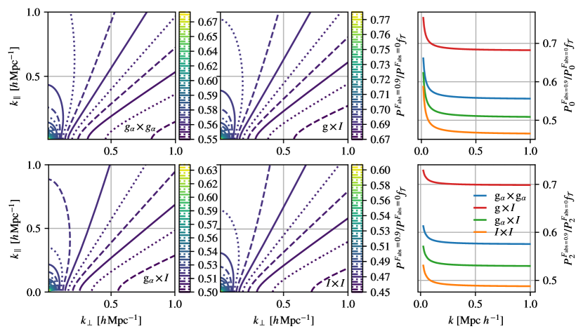
Figure 1: Effect of IGM absorption on the Ly$\alpha$ intensity power spectrum in the analytic model with $\tau_{0}=5$, $b_{I}=b_{\mathrm{g_{\alpha}}}=b_{\mathrm{g}}=1.5$, $F_{\mathrm{abs}}=0.9$, $\lambda_{\mathrm{mfp}}=300\,\mathrm{Mpc}$, and $\beta_{\phi}=1.8$. We show $P^{F_{\mathrm{abs}}=0.9}/P^{F_{\mathrm{abs}}=0.0}f_{\mathcal{T}}$, where $P^{F_{\mathrm{abs}}=0.9}$ is the power spectrum with $F_{\mathrm{abs}}=0.9$ and $P^{F_{\mathrm{abs}}=0.0}$ is that without absorption. The factor $f_{\mathcal{T}}$ accounts for the amplitude change due to the lower mean intensity and is $f_{\mathcal{T}}=I_{0}/I_{0}^{\mathrm{abs}}$ for the cross-power spectra ($\mathrm{g}\times I$ and $\mathrm{g}_{\alpha}\times I$), $f_{\mathcal{T}}=(I_{0}/I_{0}^{\mathrm{abs}})^{2}$ for the intensity auto-power spectrum ($I\times I$), and $f_{\mathcal{T}}=1$ for the LAE auto-power spectrum ($\mathrm{g}_{\alpha}\times\mathrm{g}_{\alpha}$). The four left and middle panels show the power spectrum damping as a function of wavenumber perpendicular and parallel to the LOS. The top left panel shows the damping of the LAE auto-power spectrum, the top middle panel shows that of the cross-power spectrum of Ly$\alpha$ intensity with non-LAE galaxies. The bottom left panel shows the LAE-Ly$\alpha$ intensity cross-power spectrum damping. The bottom middle panel shows the Ly$\alpha$ intensity auto-power spectrum. The top right panel shows the damping of the monopole of the LAE auto-power spectrum (blue), the non-LAE-intensity cross-power spectrum (red), the LAE-intensity cross-power spectrum (green), and the intensity auto-power spectrum (orange). The bottom right panel shows the same for the quadrupoles. Note that the anisotropy of the suppression depends strongly on the input parameters, especially the bias.

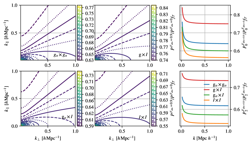
Figure 2: Same as figure 1, but with larger bias $b_{I}=b_{\mathrm{g_{\alpha}}}=b_{\mathrm{g}}=2$.

2.2 Shot noise

We have ignored the shot noise power spectrum in the previous section. Without absorption and assuming constant redshift the shot noise follows (e.g.; Bernal & Kovetz, 2022)

$$P_{\mathrm{shot}}=\frac{c}{4\pi\nu_{0}H(z)}\int_{L_{\mathrm{min}}}^{L_{\mathrm{max}}}\mathrm{d}L\,\frac{\mathrm{d}n}{\mathrm{d}L}L^{2},$$ (25)

where $\frac{\mathrm{d}n}{\mathrm{d}L}$ is the luminosity function and $L_{\mathrm{min}}$ and $L_{\mathrm{max}}$ are the minimum and maximum luminosities of the galaxies contributing to the intensity map. Assuming that the intrinsic luminosity of a galaxy is independent of the matter density and therefore uncorrelated with the local transmittance, equation (25) turns into

$$P_{\mathrm{shot}}^{\mathrm{abs}}=\frac{c}{4\pi\nu_{0}H(z)}\int_{L_{\mathrm{min}}^{\prime}}^{L_{\mathrm{max}}^{\prime}}\mathrm{d}L\,\frac{\mathrm{d}n}{\mathrm{d}L}L^{2}\mathcal{T}_{\mathrm{g}}^{2}.$$ (26)

If the galaxy sample changes, for example because only undetected galaxies contribute to the intensity map through masking, the integration limits have to be changed: $L^{\prime}_{\mathrm{min/max}}=\mathcal{T}_{g}^{-1}L_{\mathrm{min/max}}$.

3 Ly$\alpha$ Line Shift and Broadening

For Ly$\alpha$ photons to escape the ISM, they have to diffuse spatially and spectrally. In the absence of inflows or outflows, this gives rise to a symmetric, double-peaked spectrum, while simple shell models show that inflows enhance, and outflows suppress, the blue peak (e.g.; Verhamme et al., 2006). Because a sufficiently redshifted peak is redshifted out of the Ly$\alpha$ cross-section, only the blue part of the spectrum is subject to intergalactic absorption. At redshifts $z\gtrsim 2$, LAEs predominantly have red peaks (see, e.g.; Ouchi et al., 2020).

The RT in the ISM also broadens the Ly$\alpha$ line. This affects the intensity auto- and cross-power spectra in the same way as spectral smoothing of the intensity map (see, e.g.; Lujan Niemeyer et al., 2023). For modeling of the voxel intensity distribution including spectral broadening, see Bernal (2024).

When the redshift-space position of LAEs is determined from the Ly$\alpha$ line, it is affected by the line shift caused by RT as well as by the peculiar velocity of the galaxies. Following Byrohl et al. (2019), we consider the redshift-space galaxy density field that is exact under the assumption of one fixed global LOS direction $\hat{\mathbf{e}}_{\parallel}$ (Taruya et al., 2010),

$$\widetilde{\delta}_{\mathrm{g}}^{s}(\mathbf{k})=\int\mathrm{d}^{3}\mathbf{x}\left[\delta_{\mathrm{g}}(\mathbf{x})-\partial_{\parallel}u_{\parallel}(\mathbf{x})\right]e^{i\mathbf{k}\cdot\mathbf{x}+ik_{\parallel}u_{\parallel}(\mathbf{x})}.$$ (27)

Here we introduced a scaled velocity $\mathbf{u}=\mathbf{v}/(aH)$ and $\partial_{\parallel}$ denotes the derivative with respect to the LOS distance. The same equation can be written for $\widetilde{\delta I^{s}}(\mathbf{k})$. If we cross-correlate this galaxy overdensity with another field $\delta_{\mathrm{g^{\prime}}}$ that is not affected by $u_{\parallel}(\mathbf{x})$, and neglecting cross-shot noise, we can write the cross-power spectrum as

$$P^{s}_{\mathrm{gg^{\prime}}}(\mathbf{k})=\int\mathrm{d}^{3}\mathbf{r}\,e^{i\mathbf{k}\cdot\mathbf{r}}\langle e^{ik_{\parallel}u_{\parallel}(\mathbf{x})}\left[\delta_{\mathrm{g}}(\mathbf{x})-\partial_{\parallel}u_{\parallel}(\mathbf{x})\right]\delta_{\mathrm{g}^{\prime}}(\mathbf{x}^{\prime})\rangle,$$ (28)

where we have used that the expression within the angle brackets depends only on $\mathbf{r}=\mathbf{x}^{\prime}-\mathbf{x}$. We can rewrite this in terms of the cumulants as (Scoccimarro, 2004; Taruya et al., 2010; Byrohl et al., 2019)

$$\begin{split}P^{s}_{\mathrm{gg^{\prime}}}(\mathbf{k})&=\int\mathrm{d}^{3}\mathbf{r}\,e^{i\mathbf{k}\cdot\mathbf{r}}\exp\left\{\langle e^{ik_{\parallel}u_{\parallel}(\mathbf{x})}\rangle_{c}\right\}\\ &\times[\langle e^{ik_{\parallel}u_{\parallel}(\mathbf{x})}A(\mathbf{x})\delta_{\mathrm{g}^{\prime}}(\mathbf{x^{\prime}})\rangle_{c}\\ &+\langle e^{ik_{\parallel}u_{\parallel}(\mathbf{x})}A(\mathbf{x})\rangle_{c}\langle e^{ik_{\parallel}u_{\parallel}(\mathbf{x})}\delta_{\mathrm{g}^{\prime}}(\mathbf{x^{\prime}})\rangle_{c}],\end{split}$$ (29)

where $A(\mathbf{x})=\delta_{\mathrm{g}}(\mathbf{x})-\partial_{\parallel}u_{\parallel}(\mathbf{x})$. The factor $\exp\left\{\langle e^{ik_{\parallel}u_{\parallel}(\mathbf{x})}\rangle_{c}\right\}$ can be taken out of the integration because it does not depend on $\mathbf{r}$. It constitutes a Fingers-of-God-like damping of the form

$$\begin{split}D^{\mathrm{cross}}_{v_{\mathrm{RT}}}&=\exp\left\{\langle e^{ik_{\parallel}u_{\parallel}}\rangle_{c}\right\}=\langle e^{ik\mu u_{\parallel}}\rangle\\ &=\int\mathrm{d}u_{\parallel}\phi(u_{\parallel})e^{ik\mu u_{\parallel}},\end{split}$$ (30)

where $\phi(u_{\parallel})$ is the probability density function (PDF) of the LOS velocity shift $u_{\parallel}$. This factor is a one-dimensional Fourier transform of $\phi(u_{\parallel})$ to the variable $k\mu$.

As an example, consider a Gaussian PDF with mean $\bar{u}_{\parallel}$ and standard deviation $\sigma_{u_{\parallel}}$. The cross-power spectrum damping factor is then

$$D^{\mathrm{cross}}_{v_{\mathrm{RT}}}=e^{ik\mu\bar{u}_{\parallel}-\frac{1}{2}k^{2}\mu^{2}\sigma_{u_{\parallel}}^{2}},$$ (31)

which contains a phase shift due to $\bar{u}_{\parallel}$. The real component of the cross-power spectrum is therefore multiplied by

$$\Re{\left(D^{\mathrm{cross}}_{v_{\mathrm{RT}}}\right)}=\mathrm{cos}(k\mu\bar{u}_{\parallel})e^{-\frac{1}{2}k^{2}\mu^{2}\sigma_{u_{\parallel}}^{2}}.$$ (32)

The imaginary part of the power spectrum is multiplied by the respective sine function. The cosine has a zero point at $k\mu=\pi/(2\bar{u}_{\parallel})\approx 0.9\,h\mathrm{Mpc}^{-1}$ for $\bar{u}_{\parallel}=200\,\mathrm{km}\mathrm{s}^{-1}$ at $z=3$. Note that an auto-power spectrum of $\delta_{\mathrm{g}}^{s}$ will have a Fingers-of-God-like damping of the form

$$D_{v_{\mathrm{RT}}}^{\mathrm{auto}}(k,\mu)=\left|\int\mathrm{d}u_{\parallel}\phi(u_{\parallel})e^{ik\mu u_{\parallel}}\right|^{2},$$ (33)

which is unaffected by $\bar{u}_{\parallel}$ (see Byrohl et al., 2019).

The phase shift can also occur in a cross-power spectrum of two fields with different velocity distributions, such as the cross-correlation between the detected, bright LAEs with the intensity of undetected, faint LAEs as planned by the HETDEX collaboration (Lujan Niemeyer et al., 2023).

4 Lognormal simulation

4.1 Modeling

The analytic model is limited to the linear approximation of the optical depth in equation (10), which is only expected to hold for small fluctuations in the matter density, ionization rate, and velocity. However, the Ly$\alpha$ absorption mostly happens in the immediate environment of the galaxies, where these fluctuations are large.

To introduce a more accurate, but fast model, we modify the Simple code (Lujan Niemeyer et al., 2023) to include the effect of Ly$\alpha$ RT. Simple is a tool for quickly generating mock intensity maps. It uses lognormal galaxy simulations (Agrawal et al., 2017) and randomly assigns a luminosity to each galaxy by sampling from the input luminosity function. One can smooth the map, add noise, and apply sky subtraction to make the mocks more realistic for observations. One can also apply a selection function to obtain a catalog of detected galaxies.

The lognormal simulations of Agrawal et al. (2017) calculate the velocity field from the linearized continuity equation. Together with the matter density field and a model for ionization and the IGM transmittance, we can build a model for IGM absorption.

We model the ionization rate as proportional to the galaxy number density field of all (detected and undetected) galaxies, smoothed with the kernel $K_{\lambda}$ in equation (16). The amplitude of the ionization rate is chosen so that the mean ionization rate matches that of Khaire & Srianand (2019) in each redshift bin. The mean free path of ionizing photons $\lambda_{\mathrm{mfp}}$ is left as a free parameter.

We calculate the hydrogen number density field $n_{\mathrm{H}}$ to be proportional to the matter density field:

$$n_{\mathrm{H}}=\frac{\rho_{\mathrm{H}}}{m_{\mathrm{P}}}=\frac{0.75\Omega_{\mathrm{b}}{\rho}_{c}}{m_{\mathrm{P}}}\left(1+\delta_{\mathrm{m}}\right),$$ (34)

where $\rho_{\mathrm{H}}$ is the hydrogen mass density, $m_{\mathrm{P}}$ is the proton mass, $\Omega_{\mathrm{b}}$ is the baryon density parameter, $\rho_{c}$ is the critical density, and $\delta_{\mathrm{m}}$ is the matter overdensity output from the lognormal simulation.

The velocity field is calculated by the lognormal simulation of Agrawal et al. (2017). We use numpy.gradient to calculate the velocity gradient.

Finally, we calculate the local optical depth $\tau_{\delta}(\mathbf{x})$ and transmittance $\mathcal{T}(\mathbf{x})$ in each cell with equations (5) and (6). The luminosity $L(\mathbf{x})$ of each galaxy at the position $\mathbf{x}$ is replaced with $\mathcal{T}(\mathbf{x})L(\mathbf{x})=\left[1-F_{\mathrm{abs}}+F_{\mathrm{abs}}e^{-\tau_{\delta}(\mathbf{x})}\right]L(\mathbf{x})$ before generating the intensity map. $F_{\mathrm{abs}}$ is equal for all galaxies. We use this transmitted intensity map to calculate the power spectra and the transmitted flux for the selection function for the detected galaxy catalog.

Using a cosmological RT simulation, Byrohl et al. (2019) find that the Ly$\alpha$ velocity shift from RT is independent of the peculiar velocity of the host halo. We therefore model this effect by adding a random velocity shift to the mock galaxies following an input PDF $\phi(u_{\parallel})$.

Because line broadening can be modeled in the same way as a limited spectral resolution, one can increase the LOS smoothing in the input to Simple.

4.2 RT Effects in Lognormal Simulations

We set up a cubic box with length $L_{\mathrm{box}}=512\,\mathrm{Mpc}\,h^{-1}$ and $N_{\mathrm{mesh}}=256$ at mean redshift $\bar{z}=2.2$ with galaxy bias $b=1.5$ and the EWgt60 Ly$\alpha$ luminosity function of Konno et al. (2016). We adopt a constant flux limit $F_{\mathrm{min}}=3\times 10^{-18}\,\mathrm{erg}\,\mathrm{s}^{-1}$ for detection, no noise, and no smoothing of the intensity map. To remove the shot noise, we calculate the power spectrum using the half-sum-half-difference approach (HSHD; see appendix and Ando et al., 2018; Wang et al., 2022). We study the IGM absorption and the line shift effects separately.

To exaggerate the IGM absorption effect, we adopt a large absorption fraction $F_{\mathrm{abs}}=0.9$ and use all galaxies to generate the intensity map. We set the mean free path of ionizing photons to $\lambda_{\mathrm{mfp}}=300\,\mathrm{Mpc}$.

Figure 3 shows the distribution of the neutral hydrogen fraction, the optical depth, and the effective transmittance values (accounting for $F_{\mathrm{abs}}$) in the whole box compared to that in voxels containing galaxies and their mean values. The transmittance at galaxy positions is smaller than the overall mean transmittance in the simulation volume because galaxies lie in matter overdensities and therefore neutral hydrogen overdensities by construction. The mean galaxy-weighted transmittance is low, $\bar{\mathcal{T}}_{\mathrm{g}}\simeq 0.5$. The optical depth distribution has a long tail towards high optical depths. As a result, the mean optical depth is higher and inconsistent with the measurement of Turner et al. (2024), which is of order $\simeq 0.1$. The median optical depth in the lognormal simulations is lower at $\simeq 0.1$.

We calculate the intensity and LAE auto-power spectra, the LAE-Ly$\alpha$ intensity cross-power spectrum and the cross-power spectrum of Ly$\alpha$ intensity with non-Ly$\alpha$ galaxies that have an uncorrelated luminosity function and are unaffected by IGM absorption. We subtract the shot noise using the HSHD method, and take the average power spectrum of $1000$ mocks. Figure 4 shows the power spectrum ratios as a function of $k_{\perp}$ and $k_{\parallel}$ with over without IGM absorption. The main effect of the absorption is a suppression that is stronger at small scales. This is predicted by the analytic model, where the suppression is stronger at small scales where $K_{\lambda}$ is small. However, the shape of the suppression differs from the analytic model in the setup with the same bias, luminosity function slope, and mean optical depth (see Figure 1). The suppression from IGM absorption in the lognormal simulations looks similar for a bias of $b=2$ as for $b=1.5$.

To explore the reason behind this discrepancy, we calculate the transmittance according to equation (10) using $\delta_{\mathrm{m}}$, $\delta_{v}$, $\delta_{\Gamma}$, and $\tau_{0}=5$ from the lognormal simulation. Figure 5 compares this transmittance to that directly calculated from the mocks. It shows that the linear approximation for the optical depth in equation (10) does not describe the results of the lognormal simulations well. The absorption is dominated by the immediate surroundings of the galaxies, where the $\delta$ values are too large for linear approximations to hold.

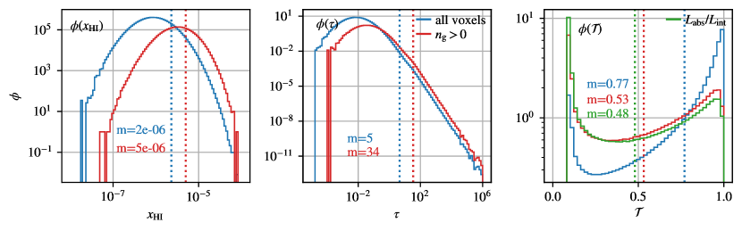
Figure 3: Distributions of the neutral hydrogen fraction $x_{\mathrm{HI}}$ (left panel), the optical depth (middle panel) and the effective transmittance with $F_{\mathrm{abs}}=0.9$ (right panel) of the entire mock box (blue) of the test mock compared to those in voxels containing at least one galaxy (red). The green line in the right panel shows the effective transmittance of the galaxies calculated from ratio of the attenuated and original luminosity. The dotted lines and the text show the corresponding mean values.

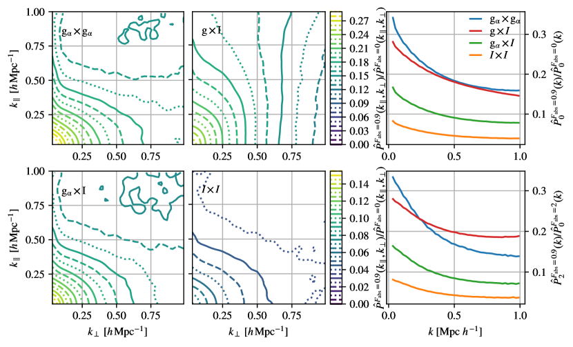
Figure 4: Similar to Figure 1, but for the lognormal mocks after shot noise subtraction. These power spectrum ratios include the decreased mean intensity. The ratios of the power spectrum with absorption ($F_{\mathrm{abs}}=0.9$) over that without absorption ($F_{\mathrm{abs}}=0$) of the LAE auto-power spectrum (top left panel), the LAE-Ly$\alpha$ intensity cross-power spectrum (bottom left panel), the non-LAE-Ly$\alpha$ intensity cross-power spectrum (top middle panel) and the intensity auto-power spectrum (bottom middle panel) are shown. The right panels show the damping of the monopole and quadrupole of the LAE auto-power spectrum (blue), the non-LAE-Ly$\alpha$ intensity cross-power spectrum (red), the LAE-Ly$\alpha$ intensity cross-power spectrum (green) and the intensity auto-power spectrum (orange). The 2D damping maps were smoothed with a Gaussian kernel with the width of $\sigma\simeq 0.024\,h\mathrm{Mpc}^{-1}$ for better visualization.

Figure 5: Transmittance calculated directly from the lognormal simulation $\mathcal{T}_{\mathrm{LN}}$ compared to that calculated with equation (10) using $\delta_{\mathrm{m}}$, $\delta_{v}$, $\delta_{\Gamma}$, and $\tau_{0}=5$ from the lognormal simulation ($\mathcal{T}_{\mathrm{WD11}}$), setting $F_{\mathrm{abs}}=1$ for both transmittance values. Darker regions contain more points, shown with a logarithmic color scale.

To model the Ly$\alpha$ line shift, we set $\phi(u_{\parallel})$ to a Gaussian PDF with mean $\bar{v}_{\mathrm{RT}}=639\,\mathrm{km}\,\mathrm{s}^{-1}$ and standard deviation $\sigma_{v_{\mathrm{RT}}}=169\,\mathrm{km}\,\mathrm{s}^{-1}$. This line shift PDF is a best-fit Gaussian to the line shift distribution at $z=3.01$ with a galaxy number density $\bar{n}_{\mathrm{g}}=10^{-3}\,\mathrm{Mpc}^{-3}h^{3}$ considering only the red peak in the RT simulation of Byrohl et al. (2019). In order to see the phase shift of the cross-power spectrum in this test, we keep the redshift-space positions of the galaxies in the galaxy catalog unchanged, while we add the line shift to the galaxies to calculate the intensity map. We use all galaxies to generate the intensity map in order to see the effect of the line shift on the cross-shot noise. We calculate the shot-noise-subtracted 2D power spectrum from an average of $100$ mocks using the HSHD method. We calculate the ratios between the power spectrum with and without the RT line shift and compute the mean damping along the LOS by averaging over $k_{\perp}$. We confirm that the cross- and auto-power spectra follow the expected damping in equations (32) and (33).

5 Sensitivity of a HETDEX-like experiment

We use the same HETDEX-like mocks as in Lujan Niemeyer et al. (2023) and include IGM absorption, a Ly$\alpha$ line shift, and Ly$\alpha$ line broadening to investigate the sensitivity of the power spectrum measured by a HETDEX-like survey to Ly$\alpha$ RT effects. We set the mean free path of ionizing photons to $\lambda_{\mathrm{mfp}}=300\,\mathrm{Mpc}$. We set $\phi(u_{\parallel})$ to a Gaussian PDF with mean $\bar{v}_{\mathrm{RT}}=639\,\mathrm{km}\,\mathrm{s}^{-1}$ and standard deviation $\sigma_{v_{\mathrm{RT}}}=169\,\mathrm{km}\,\mathrm{s}^{-1}$. Fig. 13 of Mentuch Cooper et al. (2023) shows the observed line width distribution of the LAEs in HETDEX with a mean of $\sigma_{\lambda}=3.54\,\mbox{\AA}$, which includes the intrinsic Ly$\alpha$ line width of the LAEs and the smoothing of the spectrograph VIRUS ($\sigma_{\lambda}\approx 2.38\,\mbox{\AA}$; see Hill et al., 2021). To model the line broadening through RT and the VIRUS resolution, we apply Gaussian smoothing of the intensity map along the LOS with $\sigma_{\lambda}=3.54\,\mbox{\AA}$ in the case with Ly$\alpha$ RT effects, and $\sigma_{\lambda}=2.38\,\mbox{\AA}$ in the fiducial case without RT. We subtract the shot noise using the HSHD method.

Figure 6 shows the impact of the RT effects on the HETDEX power spectra compared to the fiducial case in dashed lines at $\bar{z}=2.2$. We obtain a similar result for $\bar{z}=3.0$. The fiducial galaxy auto-power spectrum quadrupole looks slightly different than in Lujan Niemeyer et al. (2023) because the HSHD method removes some previously unaccounted-for shot noise in the quadrupole. The amplitude, i.e. the effective bias, is lower for higher $F_{\mathrm{abs}}$. The RT line shift dispersion suppresses the power spectrum at small scales, also noticeable in the different shapes of the quadrupole. The effects are significant even at $F_{\mathrm{abs}}=0.2$. Note that the covariance of the power spectra with $F_{\mathrm{abs}}>0$ is overestimated because we do not change the input luminosity function, which is measured from observed fluxes, so that the number of observed galaxies is lower than for $F_{\mathrm{abs}}=0$.

These results show that HETDEX will be affected by Ly$\alpha$ RT if such effects are present. However, because the main effect of the Ly$\alpha$ absorption is degenerate with the LAE bias, it can be difficult to isolate. Greig et al. (2013) show that the bispectrum can help break degeneracies between gravitational and RT effects. Using the power spectrum, HETDEX can nonetheless constrain the Ly$\alpha$ line shift distribution (see Section 3). Because LAEs are mostly central halo galaxies and therefore unaffected by virial motion (Ouchi et al., 2020), a Fingers-of-God-like damping with a velocity dispersion of order $\simeq 100\,\mathrm{km\,s^{-1}}$ would likely stem from RT line shifts.

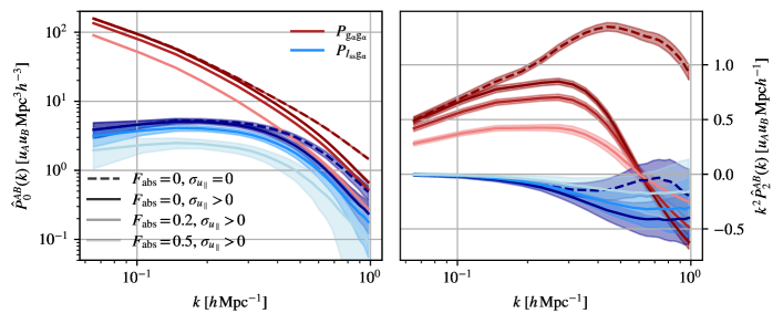
Figure 6: Power spectrum monopoles (left panel) and quadrupoles (right panel) with RT effects (solid lines) compared to the fiducial case without RT effects (dashed lines) in the $\bar{z}=2.2$ bin. The red lines show the LAE auto-power spectra and the blue lines show the cross-power spectra of LAEs with sky-subtracted intensity. The absorption fraction is shown with differently shaded lines, where lighter lines correspond to higher $F_{\mathrm{abs}}$. The shaded areas show the standard deviation of the mocks. The units are $u_{\mathrm{g_{\alpha}}}=1$ and $u_{I}=10^{-21}\,\mathrm{erg}\,\mathrm{s}^{-1}\,\mathrm{cm}^{-2}\,\mathrm{arcsec}^{-2}\,\mbox{\AA}^{-1}$.

6 Discussion

Lognormal simulations directly produce the galaxy and matter distributions and linear velocities, which we use in this work to calculate the optical depth. This approach requires an assumption of the ionization rate smoothing kernel and the Ly$\alpha$ absorption fraction, but produces the mean optical depth as output. In this regard, there are fewer free parameters than in the analytic model. While the mean optical depth is dominated by a long tail towards high optical depths and inconsistent with the measurement of Turner et al. (2024), the median optical depth is lower and consistent with the measurement.

Because the lognormal simulations do not include galaxy-scale or CGM-scale physics, the optical depth is calculated from large-scale matter distributions and velocities, so that a correlation between the optical depth and the galaxy distribution and therefore an IGM absorption effect on the power spectrum is inevitable. We showed that this approach produces high optical depths in voxels containing galaxies. As in the WD11 model, the parameter $F_{\mathrm{abs}}$ defines how much of the Ly$\alpha$ RT takes place on the scale of the resolution of the simulations ($\simeq$Mpc), where $F_{\mathrm{abs}}=0$ represents the case where no RT takes place on these scales. This means that we account for the shape of the Ly$\alpha$ line emerging from the CGM only effectively with $F_{\mathrm{abs}}$ (see equation (6)).

We find that the linear analytic model for absorption does not describe the lognormal simulations well. In the lognormal simulations, the absorption takes place in the immediate environment of the galaxies, where the matter overdensity is large. In this regime, the linear approximations for the transmittance and the effect on power spectrum break down. Therefore the linear model is an inadequate description of the effect of Ly$\alpha$ absorption on the LIM power spectra.

A minor shortcoming of the lognormal approach is that we used the same luminosity function as an input, so that fewer galaxies are detected and the mean observed intensity is lower after IGM absorption. To mitigate this, one could change the input luminosity function to match it to the observed one after absorption. One could also implement a distribution of absorption fractions, which we assume will not change the power spectra, but slightly increase the covariance. Despite the shortcomings, this is the best approach to make predictions for upcoming LAE clustering and Ly$\alpha$ LIM experiments such as HETDEX.

To summarize, the correlation between Ly$\alpha$ transmission and the large-scale matter and velocity, and therefore the effect of IGM absorption on the LAE and LIM power spectra, are model-dependent. Observations of the LAE and Ly$\alpha$ LIM power spectra, such as from HETDEX, are clearly necessary for constraints. As shown in this paper, HETDEX could be strongly affected by Ly$\alpha$ RT and will need to account for it in the power spectrum modeling.

In this work, we have only accounted for Ly$\alpha$ absorption in the IGM and Ly$\alpha$ line shifts and broadening from RT. We have not attempted to study the impact of the Ly$\alpha$ absorption from background continuum sources on Ly$\alpha$ LIM power spectra. The Ly$\alpha$ forest in quasar spectra can easily be masked by masking quasar spectra for LIM. However, Weiss et al. (2024) find broad absorption troughs around LAEs in HETDEX through stacking, which will affect Ly$\alpha$ LIM studies.

7 Summary and conclusion

We presented an analytic model for the effect of Ly$\alpha$ absorption in the IGM on the Ly$\alpha$ LIM power spectra by adapting that of WD11. While the overall effect is similar to that of the LAE auto-power spectrum - a lower, scale-dependent effective bias and reduced RSD, the suppression of the LIM component does not depend on the slope of the luminosity function.

We extended the model of Byrohl et al. (2019) of the effect of line shifts from Ly$\alpha$ RT on the galaxy power spectrum to LIM power spectra. The effect on the intensity auto-power spectrum is the same as for LAEs. In cross-correlations of one tracer affected by this line shift with another that is unaffected, a phase shift of the power spectrum is introduced, leading to a cosine-shaped damping of the real part of the power spectrum. This can be useful to measure the average line shift and its dispersion of different galaxy populations with or without LIM.

We modified the Simple code, a lognormal galaxy and intensity map simulator, to calculate the optical depth in each voxel from the matter and velocity distribution and attenuation of the intrinsic luminosities of galaxies in that voxel. In this model, a correlation between the optical depth and large-scale matter and velocity distributions is inevitable, but can be modulated with the effective absorption fraction $F_{\mathrm{abs}}$. We also add a random RT line shift to the peculiar velocities. The analytic model for the line shifts matches the results of the lognormal simulations.

While both the analytic and the lognormal models for IGM absorption predict a stronger power spectrum suppression at small scales, their predictions for the dependence of the suppression on $k_{\parallel}$ and $k_{\perp}$ differ because the linear approximations break down in the non-linear environment of the galaxies.

Finally, we implemented the modified Simple code to model the effects of Ly$\alpha$ RT on the LAE and LAE-Ly$\alpha$ intensity power spectra for a HETDEX-like experiment. The line shift and broadening from RT significantly change the monopoles and quadrupoles of the power spectra. The IGM absorption also changes the power spectra significantly even at an absorption fraction of $0.2$. Therefore, HETDEX will help constrain the interplay of Ly$\alpha$ RT and galaxy clustering. Our lognormal framework will be useful for the interpretation of upcoming large-scale structure measurements using Ly$\alpha$ emission.

Appendix A Half-Sum-Half-Difference Method for LIM

Ando et al. (2018) introduce the half-sum-half-difference (HSHD) method for galaxy clustering to automatically remove shot noise. This is especially useful if the shot noise is anisotropic or scale-dependent. One randomly splits the galaxy sample into two halves and calculates the density contrast for each, $\delta_{\mathrm{g}1}$ and $\delta_{\mathrm{g}2}$. Then one calculates the half sum (HS) and half difference (HD) of the two fields

$$\mathrm{HS}=\frac{1}{2}\left(\delta_{\mathrm{g}1}+\delta_{\mathrm{g}2}\right);\;\mathrm{HD}=\frac{1}{2}\left(\delta_{\mathrm{g}1}-\delta_{\mathrm{g}2}\right).$$ (A1)

One can then calculate

$$\langle\widetilde{\mathrm{HS}}(\mathbf{k})\,\widetilde{\mathrm{HS}}^{\ast}(\mathbf{k}^{\prime})\rangle-\langle\widetilde{\mathrm{HD}}(\mathbf{k})\,\widetilde{\mathrm{HD}}^{\ast}(\mathbf{k}^{\prime})\rangle=\left(2\pi\right)^{3}\delta_{D}(\mathbf{k}-\mathbf{k}^{\prime})P^{\mathrm{auto}}_{\mathrm{HSHD}}(\mathbf{k}),$$ (A2)

where $\delta_{D}$ is the Dirac delta function. The auto-power spectrum of HS contains the signal and shot noise, while that of HD only contains the shot noise, so that equation (A2) contains only the signal. As shorthand, we use the notation

$$\hat{P}_{\mathrm{HSHD}}^{\mathrm{auto}}=\langle\mathrm{HS}\,\mathrm{HS}^{\ast}\rangle-\langle\mathrm{HD}\,\mathrm{HD}^{\ast}\rangle.$$ (A3)

Wang et al. (2022) extend this method to the cross-power spectrum of two galaxy catalogs $A$ and $B$, where each galaxy in $A$ corresponds to a galaxy in $B$. One splits the catalogs into two halves so that $A_{1}$ and $B_{1}$ (and $A_{2}$ and $B_{2}$) maintain the one-to-one correspondence, and then calculates $\mathrm{HS}_{A/B}$ and $\mathrm{HD}_{A/B}$. The shot-noise-free cross-power spectrum estimator takes the form

$$\hat{P}_{\mathrm{HSHD}}^{\mathrm{cross}}=\langle\mathrm{HS}_{A}\mathrm{HS}^{\ast}_{B}\rangle-\langle\mathrm{HD}_{A}\mathrm{HD}^{\ast}_{B}\rangle.$$ (A4)

LIM surveys typically have low resolution, so that the separation into two galaxy samples is not possible. After all, measuring the integrated emission from all galaxies within a resolution element is the main concept of LIM. Instead of separating galaxy samples, one can still separate observations of the same volume at different times and cross-correlate these to remove the intensity noise power spectrum. The HETDEX survey, however, is not designed solely for LIM, but has a higher resolution in order to detect individual galaxies, which can be artifically decreased for LIM. In this case, it may be possible to separate galaxies within the same LIM voxel.

For modeling purposes, it is helpful to separate the clustering power spectrum from the shot noise and intensity noise. In the mock, we can randomly split the galaxies contributing to the intensity map into two separate samples and calculate $\delta I_{\mathrm{g}i}=I_{\mathrm{g}i}-\langle I_{\mathrm{g}i}\rangle$ for each sample $i$. Because only half of the galaxies contribute, the mean intensity is halved $\langle I_{\mathrm{g}i}\rangle=\frac{1}{2}\langle I_{\mathrm{all}}\rangle$. Let us assume that $I_{\mathrm{g}i}$ includes uncorrelated intensity noise with the same variance $\langle I_{\mathrm{noise}}^{2}\rangle=\sigma_{\mathrm{I}}^{2}$, so that $\langle\delta I_{\mathrm{g}i}\delta I^{\ast}_{\mathrm{g}j}\rangle=\langle\delta I_{\mathrm{g}i,\mathrm{signal}}\delta I^{\ast}_{\mathrm{g}j,\mathrm{signal}}\rangle+\sigma_{\mathrm{I}}^{2}\delta_{ij}$, where $\delta_{ij}$ is the Kronecker delta. Defining

$$\mathrm{HS}_{I}=\delta I_{\mathrm{g}1}+\delta I_{\mathrm{g}2}~{}\mathrm{and}~{}\mathrm{HD}_{I}=\delta I_{\mathrm{g}1}-\delta I_{\mathrm{g}2},$$ (A5)

the power spectrum estimator becomes

$$\begin{split}\hat{P}_{II}=\langle\mathrm{HS}_{I}\mathrm{HS}^{\ast}_{I}\rangle-\langle\mathrm{HD}_{I}\mathrm{HD}^{\ast}_{I}\rangle=2\left(\langle\delta I_{\mathrm{g}1}\delta I^{\ast}_{\mathrm{g}2}\rangle+\langle\delta I_{\mathrm{g}2}\delta I^{\ast}_{\mathrm{g}1}\rangle\right)=\frac{1}{2}\frac{\langle I_{\mathrm{all}}\rangle^{2}}{\langle I_{\mathrm{g}i}\rangle^{2}}\left(\langle\delta I_{\mathrm{g}1}\delta I^{\ast}_{\mathrm{g}2}\rangle+\langle\delta I_{\mathrm{g}2}\delta I^{\ast}_{\mathrm{g}1}\rangle\right).\end{split}$$ (A6)

The power spectrum estimator has the same normalization $\langle I_{\mathrm{all}}\rangle^{2}$ as the “normal” power spectrum estimator $\langle\delta I_{\mathrm{all}}\delta I^{\ast}_{\mathrm{all}}\rangle$. Note that $\mathrm{HS}_{i}$ and $\mathrm{HD}_{i}$ contain the intensity noise term $2\langle\sigma_{I}^{2}\rangle$, which cancels out in $\hat{P}_{II}$ as long as the intensity noise contributions of $\delta I_{\mathrm{g}1}$ and $\delta I_{\mathrm{g}2}$ are uncorrelated.

Similarly, the cross-power spectrum with a galaxy sample separated into $\delta_{\mathrm{g}1}$ and $\delta_{\mathrm{g}2}$ can be estimated as

$$\hat{P}_{I\mathrm{g}}=\langle\mathrm{HS}\,\mathrm{HS}^{\ast}_{I}\rangle-\langle\mathrm{HD}\,\mathrm{HD}^{\ast}_{I}\rangle,$$ (A7)

which does not contain shot noise as long as $\delta_{\mathrm{g}1}$ and $\delta I_{\mathrm{g}2}$ (and $\delta_{\mathrm{g}2}$ and $\delta I_{\mathrm{g}1}$) do not share galaxies contributing to both fields. This can be achieved by using the same galaxy split for $\delta_{\mathrm{g}i}$ and $\delta I_{\mathrm{g}i}$ in the mock.

The treatment of intensity noise and sky subtraction for the mocks is not straightforward. To ensure that the noise power spectrum is removed along with the shot noise, the noise maps of $\delta I_{\mathrm{g}1}$ and $\delta I_{\mathrm{g}2}$ must be uncorrelated. Depending on the split in the real data, the effective $\sigma_{I}$ of the subsamples is different than that of the total intensity. Staying agnostic, we add noise with the variance of the total intensity noise to each $\delta I_{\mathrm{g}i}$. Because the galaxy split cannot be done after the sky subtraction in the mocks, we apply the sky subtraction to each $\delta I_{\mathrm{g}i}$. In a realistic setting, the sky is subtracted before splitting the data.

References

- Agrawal et al. (2017) Agrawal, A., Makiya, R., Chiang, C.-T., et al. 2017, J. Cosmology Astropart. Phys, 2017, 003, doi: 10.1088/1475-7516/2017/10/003
- Ando et al. (2018) Ando, S., Benoit-Lévy, A., & Komatsu, E. 2018, MNRAS, 473, 4318, doi: 10.1093/mnras/stx2634
- Astropy Collaboration et al. (2013) Astropy Collaboration, Robitaille, T. P., Tollerud, E. J., et al. 2013, A&A, 558, A33, doi: 10.1051/0004-6361/201322068
- Astropy Collaboration et al. (2018) Astropy Collaboration, Price-Whelan, A. M., Sipőcz, B. M., et al. 2018, AJ, 156, 123, doi: 10.3847/1538-3881/aabc4f
- Bartelmann (2021) Bartelmann, M. 2021, Theoretical Astrophysics: An Introduction, Lecture Notes (Heidelberg University Publishing), doi: 10.17885/heiup.822
- Behrens et al. (2018) Behrens, C., Byrohl, C., Saito, S., & Niemeyer, J. C. 2018, A&A, 614, A31, doi: 10.1051/0004-6361/201731783
- Behrens & Niemeyer (2013) Behrens, C., & Niemeyer, J. 2013, A&A, 556, A5, doi: 10.1051/0004-6361/201321172
- Bernal (2024) Bernal, J. L. 2024, Phys. Rev. D, 109, 043517, doi: 10.1103/PhysRevD.109.043517
- Bernal & Kovetz (2022) Bernal, J. L., & Kovetz, E. D. 2022, A&A Rev., 30, 5, doi: 10.1007/s00159-022-00143-0
- Bolton & Haehnelt (2007) Bolton, J. S., & Haehnelt, M. G. 2007, MNRAS, 382, 325, doi: 10.1111/j.1365-2966.2007.12372.x
- Burgess (1965) Burgess, A. 1965, MmRAS, 69, 1
- Byrohl et al. (2019) Byrohl, C., Saito, S., & Behrens, C. 2019, MNRAS, 489, 3472, doi: 10.1093/mnras/stz2260
- Croft et al. (2018) Croft, R. A. C., Miralda-Escudé, J., Zheng, Z., Blomqvist, M., & Pieri, M. 2018, MNRAS, 481, 1320, doi: 10.1093/mnras/sty2302
- Croft et al. (2016) Croft, R. A. C., Miralda-Escudé, J., Zheng, Z., et al. 2016, MNRAS, 457, 3541, doi: 10.1093/mnras/stw204
- Draine (2011) Draine, B. T. 2011, Physics of the Interstellar and Intergalactic Medium
- Gebhardt et al. (2021) Gebhardt, K., Mentuch Cooper, E., Ciardullo, R., et al. 2021, ApJ, 923, 217, doi: 10.3847/1538-4357/ac2e03
- Greig et al. (2013) Greig, B., Komatsu, E., & Wyithe, J. S. B. 2013, mnras, 431, 1777, doi: 10.1093/mnras/stt292
- Gurung-López et al. (2020) Gurung-López, S., Orsi, Á. A., Bonoli, S., et al. 2020, MNRAS, 491, 3266, doi: 10.1093/mnras/stz3204
- Harris et al. (2020) Harris, C. R., Millman, K. J., van der Walt, S. J., et al. 2020, Nature, 585, 357, doi: 10.1038/s41586-020-2649-2
- Hill et al. (2021) Hill, G. J., Lee, H., MacQueen, P. J., et al. 2021, AJ, 162, 298, doi: 10.3847/1538-3881/ac2c02
- Hui & Gnedin (1997) Hui, L., & Gnedin, N. Y. 1997, MNRAS, 292, 27, doi: 10.1093/mnras/292.1.27
- Kaiser (1987) Kaiser, N. 1987, MNRAS, 227, 1, doi: 10.1093/mnras/227.1.1
- Khaire & Srianand (2019) Khaire, V., & Srianand, R. 2019, MNRAS, 484, 4174, doi: 10.1093/mnras/stz174
- Konno et al. (2016) Konno, A., Ouchi, M., Nakajima, K., et al. 2016, ApJ, 823, 20, doi: 10.3847/0004-637X/823/1/20
- Lin et al. (2022) Lin, X., Zheng, Z., & Cai, Z. 2022, ApJS, 262, 38, doi: 10.3847/1538-4365/ac82e8
- Lujan Niemeyer et al. (2023) Lujan Niemeyer, M., Bernal, J. L., & Komatsu, E. 2023, ApJ, 958, 4, doi: 10.3847/1538-4357/acfef4
- Mentuch Cooper et al. (2023) Mentuch Cooper, E., Gebhardt, K., Davis, D., et al. 2023, ApJ, 943, 177, doi: 10.3847/1538-4357/aca962
- Nakajima et al. (2018) Nakajima, K., Fletcher, T., Ellis, R. S., Robertson, B. E., & Iwata, I. 2018, MNRAS, 477, 2098, doi: 10.1093/mnras/sty750
- Ouchi et al. (2020) Ouchi, M., Ono, Y., & Shibuya, T. 2020, ARA&A, 58, 617, doi: 10.1146/annurev-astro-032620-021859
- Partridge & Peebles (1967) Partridge, R. B., & Peebles, P. J. E. 1967, ApJ, 147, 868, doi: 10.1086/149079
- Scoccimarro (2004) Scoccimarro, R. 2004, Phys. Rev. D, 70, 083007, doi: 10.1103/PhysRevD.70.083007
- Shoji et al. (2009) Shoji, M., Jeong, D., & Komatsu, E. 2009, ApJ, 693, 1404, doi: 10.1088/0004-637X/693/2/1404
- Taruya et al. (2010) Taruya, A., Nishimichi, T., & Saito, S. 2010, Phys. Rev. D, 82, 063522, doi: 10.1103/PhysRevD.82.063522
- Torrado & Lewis (2019) Torrado, J., & Lewis, A. 2019, Cobaya: Bayesian analysis in cosmology, Astrophysics Source Code Library, record ascl:1910.019
- Torrado & Lewis (2021) —. 2021, J. Cosmology Astropart. Phys, 2021, 057, doi: 10.1088/1475-7516/2021/05/057
- Turner et al. (2024) Turner, W., Martini, P., Göksel Karaçaylı, N., et al. 2024, arXiv e-prints, arXiv:2405.06743, doi: 10.48550/arXiv.2405.06743
- Verhamme et al. (2006) Verhamme, A., Schaerer, D., & Maselli, A. 2006, A&A, 460, 397, doi: 10.1051/0004-6361:20065554
- Wang et al. (2022) Wang, Y., Zhao, G.-B., Koyama, K., et al. 2022, arXiv e-prints, arXiv:2202.05248, doi: 10.48550/arXiv.2202.05248
- Weiss et al. (2024) Weiss, L. H., Davis, D., Gebhardt, K., et al. 2024, ApJ, 962, 102, doi: 10.3847/1538-4357/ad1b51
- Wyithe & Dijkstra (2011) Wyithe, J. S. B., & Dijkstra, M. 2011, MNRAS, 415, 3929, doi: 10.1111/j.1365-2966.2011.19007.x
- Zheng et al. (2011) Zheng, Z., Cen, R., Trac, H., & Miralda-Escudé, J. 2011, ApJ, 726, 38, doi: 10.1088/0004-637X/726/1/38