Amplitude-noise-resilient entangling gates for trapped ions

Abstract

Noise resilience of quantum information processing is a crucial precondition to reach the fault-tolerance threshold. While resilience to many types of noise can be achieved through suitable control schemes, resilience to amplitude noise seems to be elusive within the common harmonic approximation for the bus mode of trapped ions. We show that weak an-harmonicities admit control schemes that achieve amplitude noise-resilience consistent with state-of-the-art experimental requirements, and that the required an-harmonicities can be achieved with current standards of micro-structured traps or even the intrinsically an-harmonic Coulomb interaction.

Trapped ions are a leading candidate for the development of practical hardware for quantum computation. While proof of principle demonstrations of quantum gates exist for a variety of platforms [1, 2, 3, 4], any practical device will require a certain level of noise-resilience so that the benefits of using a quantum instead of a classical computer are not lost to the effort required for highly accurate and frequent system calibration [5, 6, 7, 8]. Existing demonstrations of resilience of trapped-ion quantum gates against fluctuations of a variety of quantities [9, 10, 11, 12, 13, 14, 15] put trapped ion quantum information much closer to practicality than many competing platforms.

By design, most of the currently employed quantum gates are resilient to fluctuations in the initial state of the ions’ motion [16, 17, 2]. Resilience against motional heating and fluctuations in the ions’ confining potential or carrier frequency of driving fields used to realize gates can be achieved in term of suitably tailored temporal shapes of the driving fields [18, 19, 20, 15, 14]. A crucial system parameter that has proven tricky to achieve noise resilience against is the amplitude of driving fields; but typical fluctuations in Rabi-frequency are in the range of a few percents.

The linear spatial dynamics of the ions is conflicting with resilience against amplitude fluctuations of driving fields. The required nonlinearity can be obtained from the intrinsically nonlinear light-matter interaction [21] beyond the Lamb-Dicke approximation. As we will show here, it is possible to achieve resilience against amplitude fluctuations, without the strong driving required for sizeable nonlinearity in the light-matter interaction, using anharmonicities in trapping potential or even the fundamentally anharmonic Coulomb interaction. Even though such anharmonicities impair resilience to thermal excitations, they do so only to an extent that can be reclaimed with the choice of temporal profile of the driving fields. With the explicit design of gate electrodes, we underpin the experimental feasibility of the weakly anharmonic trapping potential required for the present gate scheme.

The Hamiltonian of a pair of trapped ions with off-resonant driving on a red and a blue sideband is given by [16]

$$H(t)=H_{0}+\Omega_{R}\left(f(t)a^{\dagger}+af^{\ast}(t)\right)S_{y}\ ,$$ (1)

where $S_{y}=\sigma_{y}^{1}+\sigma_{y}^{2}$ is the $y$–component of the total spin operator, $a$ and $a^{\dagger}$ are the annihilation and creation operator of the bus mode; $\Omega_{R}$ is the Rabi frequency for the utilized side-band transitions, and the function $f(t)$ includes the time-dependence of the carrier frequencies of the driving fields and any time-dependence resultant from pulse shaping. $H_{0}$ is the non-interacting Hamiltonian of the internal, qubit degrees of freedom of the ions and the bus mode.

In the case of a perfectly harmonic bus mode, the impact of the non-interacting part $H_{0}$ of the system Hamiltonian reduces to an oscillatory time-dependence of the annihilation and creation operators $a$ and $a^{\dagger}$. The system Hamiltonian in the interaction picture thus reads $\tilde{H}(t)=\Omega_{R}(\tilde{f}(t)a^{\dagger}+a\tilde{f}^{\ast}(t))S_{y}$ with a driving function $\tilde{f}(t)$ dressed with the time-dependence of the non-interacting dynamics.

The gate dynamics can be represented by translation in phase space along a closed loop with length proportional to $\Omega_{R}$ [16, 17]. The Rabi-angle $\Phi_{R}$ of the effective $S_{y}^{2}$–interaction in the dynamics induced by $\tilde{H}(t)$ is given by the area enclosed by the loop, thus exhibiting the quadratic dependence $\Phi_{R}=\Omega_{R}^{2}\imaginary\int_{0}^{T}d\tau\tilde{f}(\tau)\int_{0}^{\tau}d\tau^{\prime}\tilde{f}^{\ast}(\tau^{\prime})$ [18]. The dependence of $\Phi_{R}$ on the driving pattern factorizes into an amplitude term $\Omega_{R}^{2}$ and a factor with the detailed time-dependence of the driving. There is thus no possibility of choosing driving patterns $f(t)$ that could modify the quadratic dependence on the Rabi-frequency and any fluctuation of $\Omega_{R}$ will unavoidably result in the corresponding fluctuation of the Rabi-angle $\Phi_{R}$.

In the case of an anharmonic bus mode, however, the interplay between the interaction and the non-interacting dynamics can break this factorization, and it is possible to achieve resilience against fluctuations in the Rabi frequency $\Omega_{R}$ in terms of suitably tailored driving patterns $f(t)$.

The ideal entangling gate for the qubit degrees of freedom that can be realised with the Hamiltonian $H(t)$ (Eq. (1)) is given by

$$U_{T}=\exp\left(i\frac{\pi}{8}S_{y}^{2}\right)\ .$$ (2)

Since any level of anharmonicity will restrict a gate functionality to a limited range of initial motional states, it is essential to define a gate fidelity for the joint dynamics $V$ of qubits and bus mode that takes into account this range. For any projector $P$ onto a subspace of the full Hilbert space of the bus mode, one can define

$$F(V,U_{T},P)=\left|\mbox{tr}((U_{T}^{\dagger}\otimes P)V)/(4\tr P)\right|^{2},$$ (3)

as the fidelity of a unitary $V$ for the full system of qubits and bus mode with respect to the desired gate $U_{T}$ of the qubits and the desired trivial dynamics of the bus mode within the subspace given by $P$. Resilience against amplitude fluctuations is characterized in terms of an averaged infidelity

$$I=1-\langle F(V(\Omega_{R}),U_{T},P)\rangle_{\Omega_{R}}\ ,$$ (4)

where $V(\Omega_{R})$ is the system dynamics obtained for a given Rabi frequency $\Omega_{R}$ which varies in the error range $\Omega_{C}-\delta\Omega\leq\Omega_{R}\leq\Omega_{C}+\delta\Omega$ ,where $\Omega_{C}$ is the central value and $\delta\Omega$ the error magnitude.

Although the anharmonicity can be induced by any higher order terms in the potential, for clarity the remaining discussion focuses on the quartic potential $\frac{1}{2}m\omega^{2}\left(z^{2}+z^{4}/\xi^{2}\right)$ for the bus mode, where $\xi$ is the length scale on which the potential becomes anharmonic. The perturbative correction to the COM mode’s eigen-frequencies resultant from the anharmonicity is given by $\chi n(n-1)$ with the phonon number $n$ and the scalar prefactor

$$\chi=\frac{3\hbar}{4m\xi^{2}}$$ (5)

referred to as the anharmonicity in the following.

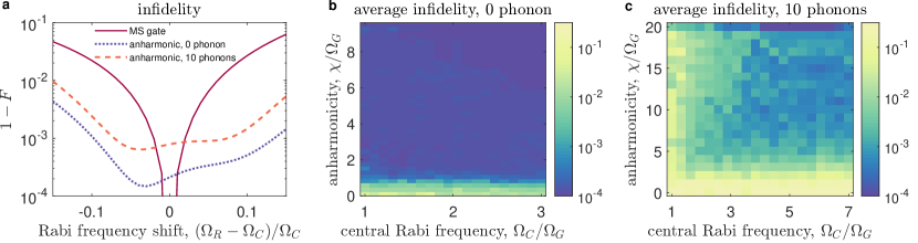
Figure 1: (a) Dependence of infidelity on Rabi frequency’s variation for the MS gate (solid red), anharmonic gate with no phonon excitation (for $\chi=2\Omega_{G},\Omega_{C}=\Omega_{G}$, dotted blue), and 10 phonon excitations (for $\chi=10\Omega_{G},\Omega_{R}=2.6\Omega_{G}$, dashed orange); here $\Omega_{G}=2\pi/T$ is the gate frequency. (b) Infidelity averaged over a 10% error range of the Rabi frequency for no phonon excitation and (c) up to 10 phonon excitations, as a function of the anharmonicity and central Rabi frequency. The optimisation is terminated once the infidelity drops below $10^{-4}$.

Driving functions $f(t)$ in Eq. (1) can be designed with common pulse-shaping algorithms [22, 23, 24] based on an ensemble of Hamiltonians of the form of Eq. (1), with each ensemble member characterized by its value of $\Omega_{R}$, but with all ensemble members having the same driving function $f(t)$. In the following, we will pursue such a numerically exact approach (given $H(t)$ in Eq. (1)), and an approximate analytic approach that is applicable to the regime of strong anharmonicities. The latter approach provides an intuitive understanding of the functionality of the control scheme, and using its driving functions as initial condition for the iterative refinement of the former approach helps to avoid sub-optimal extrema.

Fig. 1a depicts the infidelity $1-F$ (Eq. (3)) for several gates as function of the Rabi frequeny $\Omega_{R}$. The solid red curve corresponds to a perfectly harmonic system in which no resilience can be achieved, and the infidelity grows quickly with increasing deviation $|\Omega_{R}-\Omega_{C}|$ of the Rabi frequency from its ideal value. The other two curves corresponds to an anharmonic system, showing the fidelities obtained with driving patterns optimized for an equally spaced grid of Rabi frequencies in the interval $[9/10\ \Omega_{C},11/10\ \Omega_{C}]$ centered around the central Rabi frequency $\Omega_{C}$. The pulses are optimised under the constraint $|f(t)|\leq 1$. The dotted blue refers to gate fidelities with no phonon in the initial states, i.e., $P=\outerproduct{0}{0}$ in Eq. (3), for an anharmonicity $\chi=\Omega_{G}$ where $\Omega_{G}=2\pi/T$ is the gate frequency with $T$ the gate duration. The dashed orange refers to the case with up to 10 phonons, $P=\sum_{n=0}^{10}\outerproduct{n}{n}$, and anharmonicity $\chi=10\Omega_{G}$. The value of the gate frequency is chosen to be $\Omega_{G}=\Omega_{C}$ for the former gate; given the broad range of initial states, the latter gate requires a slightly lower gate frequeny $\Omega_{G}=\Omega_{C}/2.6$ in order to achieve the resilience shown in Fig. 1a.

A more quantitative picture of the noise-resilience is provided by the average infidelity $I$ (Eq. (4)). Figures  1b and c depict $I$ as function of the central Rabi frequency $\Omega_{C}$ and the anharmonicity $\chi$ for the cases of 0 phonon and up to 10 phonons in the initial states, respectively. Both insets show sub-optimal infidelities for vanishing anharmonicity, as expected. With increasing anharmonicity, however, the infidelities decrease and the threshold $10^{-4}$ is achieved in the strong anharmonicity limit. This decrease is faster in inset (c) than in inset (b), highlighting that the required anharmonicity increases with the dimension of the subspace to which its initial motional state is confined. While a Rabi frequency of value $\Omega_{R}=\Omega_{G}$ is enough to realize a fully entangling gate in the absence of amplitude fluctuations, Fig. 1 b and c also show that – depending on the desired infidelity – slightly larger Rabi-frequencies can be required in order to realize resilient gates. In particular, the required anharmonicity for achieving an average fidelity of 99.9% rises linearly when the error magnitude increases from 1% to 5%, but almost saturates for error from 5% to 10% (Supp. Mat. Sec. 3).

In order to understand the physical origin of the robustness against fluctuations in the Rabi frequency $\Omega_{R}$, it is instructive to pursue an approximate treatment that is valid for large anharmonicity, a regime, in which a transition between any pair of Fock states can be driven on resonance without sizeable off-resonant transitions between other pairs. The realization of a gate that works with an initial motional state in the subspace spanned by the lowest $N$ Fock states requires a driving profile with components $g_{n}(t)$ close-to-resonant with the transition between one pair of Fock states each (Eq. (S7) in Supp. Mat.). With such a driving profile, the system Hamiltonian in the interaction picture is approximated (in rotating wave approximation) as

$$H_{I}=\Omega_{R}\!\sum_{n=1}^{N}\sqrt{n}\Bigl{(}g_{n}(t)\sigma_{n}^{\dagger}+\sigma_{n}g_{n}^{\ast}(t)\Bigr{)}S_{y},$$ (6)

with $\sigma_{n}=\outerproduct{n-1}{n}$. The operators

$$X_{n}=\frac{1}{2}(\sigma_{n}+\sigma_{n}^{\dagger})S_{y}\ ,\mbox{ and }Y_{n}=\frac{i}{2}(\sigma_{n}-\sigma_{n}^{\dagger})S_{y}$$ (7a)

satisfy the commutation relation $$[X_{n},Y_{n}]=2iZ_{n}$$ with

$$Z_{n}=\frac{1}{4}[\sigma_{n}^{\dagger},\sigma_{n}]S_{y}^{2}\,$$ (7b)

and cyclic permutations (as $S_{y}^{3}=4S_{y}$) i.e. the same commutation relations as the Pauli operators. The dynamics with driving of a single transition is thus equivalent to that of a single qubit.

If the dynamics $V$ of qubit degrees of freedom and bus mode satisfies the relation

$$V(\bm{1}\otimes P)=\exp\left(-i\frac{\pi}{2}\sum_{n=1}^{N}nZ_{n}\right)(\bm{1}\otimes P)\ ,$$ (8)

then the desired gate for initial motional states in the subspace $P=\sum_{n=0}^{N-1}\ket{n}\bra{n}$ is realised, and thus the infidelity $I$ (Eq. (3)) is minimized. Such dynamics can be realised in terms of a sequence of steps in which a single transition is driven with a driving function $g_{n}$ that is optimized for the target dynamics $\exp\left(-in\pi/2\,Z_{n}\right)$, or any other target within $2\pi$-periodicity. In fact, since the dynamics resultant from driving profile $g_{n}(t)$ commutes with the dynamics resultant from driving profile $g_{m}(t)$ for $|n-m|>1$, such a driving scheme can be comprised of two steps only with $g_{n}=0$ for all even $n$ in one step, and $g_{n}=0$ for all odd $n$ in the other step.

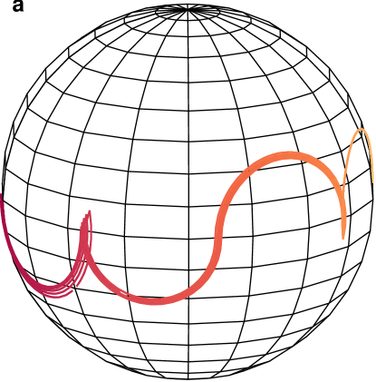
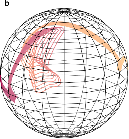
Figure 2: (a) The trajectories of the Bloch vector in the strong anharmonicity limit with the analytic pulse sequence of Eq. (9), for Rabi frequency varying in a 10% error range. The color gradient depicts temporal evolution from bright orange for the initial vector $[1,0,0]$ to dark red for the final vector $[-1,0,0]$. (b) Similar trajectories for a finite anharmonicity, $\chi=2\Omega_{G}$, and a 10% error range in the Rabi frequency. The trajectories shown are projections in the subspace of the lowest two levels, thus residing inside the Bloch sphere.

A possible choice for each of the driving functions $g_{n}(t)$ that achieves the desired resilience to amplitude noise is given by the simple piecewise constant driving function with four segments $\mathfrak{g}_{j}$, for $(j-1)T/4\leq t<jT/4$ [25], with

$$\mathfrak{g}_{1}=\mathfrak{g}_{4}^{\ast} = \frac{2\pi i}{\sqrt{n}\,\Omega_{C}T}\exp(-i\frac{3\phi}{4})\ ,$$

$$\mathfrak{g}_{2}=\mathfrak{g}_{3}^{\ast} = \frac{2\pi i}{\sqrt{n}\,\Omega_{C}T}\exp(-i\frac{\phi}{4})\ .$$ (9)

This driving pattern for $g_{n}(t)$ results in the gate $\exp(i\phi Z_{n})$ at the final time $T$ given a central Rabi-frequency with the value $\Omega_{C}$. Fluctuations in the Rabi-frequency contribute only quadratically to the gate angle and deviations from the type of gate (i.e. induced by $Z_{n}$) are of third order in Rabi-frequency fluctuations. That is, the gate is resilient to amplitude fluctuations up to second order, resulting in a robustness up to fourth order in the gate fidelity.

Fig. 2a depicts trajectories on the Bloch sphere (defined in terms of $X_{1}$, $Y_{1}$ and $Z_{1}$ for the dynamics induced by the analytic pulse sequence in Eq. (9) with $\phi=\pi/2$. Trajectories for relative Rabi frequencies $\Omega_{R}/\Omega_{C}$ from $0.9$ to $1.1$ in steps of $0.025$ are shown. The color gradient indicates the temporal evolution with bright orange for $t=0$ to dark red for $t=T$. The trajectories diverge at first due to variation in the Rabi frequency, but converge toward the end, demonstrating the robustness of the gate.

Outside the regime of strong anharmonicity and weak driving, the separation into dynamics in distinct two-dimensional subspaces breaks down. A complete representation of the actual dynamics would require an $N^{2}-1$ dimensional generalized Bloch vector. Yet, a three-dimensional projection of this generalized Bloch vector can still provide partial information. Fig. 2b shows the trajectories for such a projection (onto $X_{1}$, $Y_{1}$ and $Z_{1}$), with opacity representing the length of the projected vector for the dynamics resultant from numerically optimized driving for $\chi=2\Omega_{G}$. Due to the weaker anharmonicity as compared to inset a, the trajectories deviate more strongly during the dynamics, but they nicely refocus towards the gate time.

The required anharmonicity in the present scheme is on the order of $2\pi/T$ (see Supp. Mat. Sec. 3). With a gate time of 1ms, an-harmonicities on the order of $\chi\simeq 2\pi\times 1$kHz are sufficient to achieve resilience to amplitude fluctuations of a few quantitative percents. For a typical trap frequency in the range $2\pi\times 100$kHz - $2\pi\times 1$MHz, the coupling between different motional modes resultant from the anharmonicity is well negligible, so that the reduction of the motional dynamics to only the bus mode is well justified [26]. For the COM mode, the anharmonicity can be induced by a quartic potential in a trap geometry where the DC control electrodes are placed directly underneath the ions [27]. The anharmonicity scales as the inverse of the square of the separation between the electrodes and thus can be enhanced by reducing the size of the device [27]. However, it is more advantageous to use the stretch mode to achieve the required anharmonicity as the intrinsic anharmonic Coulomb interaction can produce a substantial anharmonicity even in a purely harmonic potential. As discussed in more detail in Supp. Mat. Sec. 1, anharmonicities around $2\pi\times 100$Hz are readily achievable via the intrinsic Coulomb interaction, and values exceeding $2\pi\times 1$kHz can be obtained with the addition of a small quantitative quartic component in the trap potential.

While they are discussed here for the specific platform of trapped ions, both the problem of amplitude fluctuations and the foundations of the presently proposed solution are prevalent in many quantum technological platforms: interactions between superconducting qubits for example can be mediated via weakly anharmonic qubit couplers [28] and long-range interactions are frequently realized via coupling to a shared cavity mode [29, 30, 31]. With intrinsic or engineered anharmonicities, all such systems can benefit from the noise-resilience that can be achieved with control techniques following the principles exemplified here with the specific example of trapped ions. The present techniques thus do not only help to bring trapped ion technology closer to the error-correction threshold, but they can find application in a broad platform of emerging technologies.

I Acknowledgements

This work was supported by the U.K. Engineering and Physical Sciences Research Council via the EPSRC Hub in Quantum Computing and Simulation (EP/T001062/1), the UK Innovate UK (project number 10004857), the US Army Research Office (W911NF21-1-0240), the US Office of Naval Research under Agreement No. N62909-19-1-2116. S.A.K. acknowledges support from an EPSRC Centre for Doctoral Training (EP/S023607/1).

Supplementary Materials

I.1 1. Anharmonicity estimation

Here we estimate the anharmonicty for the COM mode and the stretch mode in the quartic potential

$$V(z)=\frac{m\omega^{2}}{2}(z^{2}+z^{4}/\xi^{2}).$$ (S1)

For the COM mode, the effective potential is the same as that of a single trapped ion. The level shift is estimated by perturbation theory $m\omega^{2}\bra{n}z^{4}\ket{n}/2\xi^{2}$, giving $(n^{2}+n)\hbar\chi$ where $\chi=3\hbar/(4m\xi^{2})$. We write this as $\hbar\Delta_{n}+2n\hbar\chi$ where $\Delta_{n}=(n^{2}-n)\chi$ and group the second term into the harmonic part of the energy spectrum, redefining $\omega$ as the transition between the shifted ground and first excited levels.

For the stretch mode the potential energy of the system is

$$V(z)=\frac{ke^{2}}{2z}+m\omega^{2}\left(z^{2}+z^{4}/\xi^{2}\right),$$ (S2)

where $\pm z$ are the axial positions of the two ions. The equilibrium separation is given by $d_{0}=2z_{0}$ where $z_{0}$ is given by $V^{\prime}(z_{0})=0$, which yields

$$-\frac{L\,l}{2z_{0}^{2}}+2\frac{z_{0}}{l}+4\frac{z_{0}^{3}}{\xi^{2}l}=0.$$ (S3)

where $l=\sqrt{\hbar/m\omega}$ is the harmonic oscillator length and $L$ the range of the Coulomb interaction defined by $L=ke^{2}/\hbar\omega$. This equation is solved numerically. Let $\eta_{z}$ be the small displacement in the stretch mode, i.e., the positions of the ions are $z=\pm(z_{0}+\eta_{z})$, we expand the potential $V(z)$ up to the fourth order in $\eta_{z}$ to obtain

$$\frac{V(\eta_{z})}{\hbar\omega}=\left(1+\frac{L\,l^{2}}{2z_{0}^{3}}+\frac{6z_{0}^{2}}{\xi^{2}}\right)\left(\frac{\eta_{z}}{l}\right)^{2}-\left(\frac{L\,l^{3}}{z_{0}^{4}}-\frac{4z_{0}l}{\xi^{2}}\right)\left(\frac{\eta_{z}}{l}\right)^{3}+\left(\frac{L\,l^{4}}{2z_{0}^{5}}+\frac{l^{2}}{\xi^{2}}\right)\left(\frac{\eta_{z}}{l}\right)^{4}.$$ (S4)

As the total energy is $m\dot{\eta}_{z}^{2}+V(\eta_{z})$, the effective potential for the motion of the stretch mode is $V_{\text{eff}}(\eta_{z})=V(\eta_{z})/2.$ Using perturbation theory to estimate the anharmonic shift for this potential is not straightforward as the second order contribution of the cubic term can dominate the first order contribution of the quartic term. Therefore we compute the lowest three energies numerically with the Numerov method, and obtain the anharmonicity shift by $\chi=(E_{2}-E_{1})-(E_{1}-E_{0}).$

Figure S1 shows the anharmonicity for two Yb⁺ ions with mass $m=171$u in a potential with trapping frequencies, $\omega/2\pi$, varying from $0.1$ to $10$MHz and characteristic lengths, $\xi$, from $0.1$ to $1000\mu$m. There are two distinct contributions to the anharmonicity: the intrinsic anharmonicity of the Coulomb potential which increases with $\omega$, and the external anharmonicity from the trapping potential which increases with $1/\xi^{2}$. In the purely harmonic limit where $\xi$ is very large, anharmonicity $\chi\simeq 2\pi\times 100$Hz is achieved for $\omega\simeq 2\pi\times 5$MHz. The required trap frequency can be reduced with an addition of a small quartic component in the potential. In Fig. S2a we show the current design for one of our trap where the control voltage on the electrodes can be configured to create a quartic component in the potential. Fig. S2b shows a potential obtained with BEM simulation. The trap frequency, $\omega\simeq 2\pi\times 100$Hz, and characteristic length, $\xi\simeq 2\mu$m, of this potential correspond to an anharmonicity $\chi\simeq 2\pi\times 1$kHz. For comparison, the anharmonicity for the COM mode in the same quartic potential is only $3\hbar/(4m\xi^{2})\simeq 2\pi\times 10$Hz.

Figure S1: Dependence of the stretch mode’s anharmonicity on the trap frequency and the characteristic length of the quartic potential.

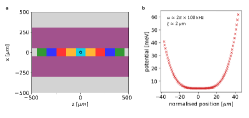
Figure S2: a) Geometry of a surface ion trap with control electrodes placed directly underneath the central trapping axis, in between the RF electrodes (purple). Five different voltages are applied symmetrically to 9 control electrodes (cyan, orange, red, blue, green) to produce an axial potential with quadratic and quartic terms at the ion location (black circle). The quartic component can be enhanced by reducing the separations between the electrodes. b) Potential curve obtained with BEM simulation. The maximum voltage on the electrodes (outside the range shown in the figure) is 70V.

I.2 2. Hamiltonian in the strong anharmonicity limit

The control Hamiltonian in the rotating frame of the free spin terms and the harmonic motional term, is then

$$\tilde{H}(t)\approx\sum_{n=0}^{\infty}\Delta_{n}\ket{n}\bra{n}+\Omega_{R}\left[\tilde{f}^{*}(t)a+a^{\dagger}\tilde{f}(t)\right]S_{y}.$$ (S5)

The interaction Hamiltonian in the rotating frame of $\sum_{n}\Delta_{n}\ket{n}\bra{n}$ is

$$\tilde{H}_{1}(t)\approx\, \Omega_{R}\sum_{n=0}^{\infty}\sqrt{n}\Big{[}\tilde{f}^{*}(t)e^{-i(\Delta_{n}-\Delta_{n-1})t}\ket{n-1}\!\bra{n}$$

$$+\ket{n}\!\bra{n-1}\tilde{f}(t)e^{i(\Delta_{n}-\Delta_{n-1})t}\Big{]}S_{y}.$$ (S6)

In the strong anharmonicity limit where the anharmonicity is much larger than the Rabi frequency of the drive, we consider a polychromatic control of the form

$$\tilde{f}(t)=\sum_{n=1}^{N-1}g_{n}(t)e^{-i(\Delta_{n}-\Delta_{n-1})t},$$ (S7)

where $g_{n}(t)$ are slowly varying on the time scale $1/(\Delta_{n}-\Delta_{n-1})$. The control Hamiltonian reads, after neglecting the counter rotating terms,

$$\tilde{H}_{2}(t)\approx\Omega_{R}\sum_{n=1}^{N}\sqrt{n}[g_{n}^{R}(t)X_{n}-g_{n}^{I}(t)Y_{n}]S_{y},$$ (S8)

where $g_{n}^{R}(t)$ and $g_{n}^{I}(t)$ are the real and imaginary parts of $g_{n}(t)$.

I.3 3. Optimisation

We used piece-wise control signals so that the control variables are the set of amplitudes for each time bin. We compute the fidelity and its gradient and optimise the fidelity using a gradient based optimisation method. We start with the strong anharmonicity limit where we find the optimal $g_{n}$, and use the solution in Eq. (S7) as an initial guess to find the optimal $\tilde{f}(t)$ for lower anharmonicity, for which the control Hamiltonian is given in Eq. (I.2).

The required anharmonicity for achieving a sufficiently low average infidelity in the error range increases with increasing error magnitude. Figure S3 shows the minimum anharmonicity needed for achieving an average infidelity below $10^{-3}$ for the cases of 0 phonon and 10 phonon excitations in the initial state. The anharmonicity rises with the error magnitude as expected but almost saturates at $5\%$.

Figure S3: Required anharmonicity for achieving an average infidelity of $10^{-3}$ w.r.t. error magnitude.

References

- Ladd et al. [2010] T. D. Ladd, F. Jelezko, R. Laflamme, Y. Nakamura, C. Monroe, and J. L. O’Brien, Quantum computers, Nature 464, 45 (2010).
- Leibfried et al. [2003] D. Leibfried et al., Experimental demonstration of a robust, high-fidelity geometric two ion-qubit phase gate, Nature 422, 412 (2003).
- He et al. [2019] Y. He, S. K. Gorman, D. Keith, L. Kranz, J. G. Keizer, and M. Y. Simmons, A two-qubit gate between phosphorus donor electrons in silicon, Nature 571, 371 (2019), publisher: Nature Publishing Group.
- Google AI Quantum et al. [2020] Google AI Quantum, B. Foxen, et al., Demonstrating a Continuous Set of Two-Qubit Gates for Near-Term Quantum Algorithms, Physical Review Letters 125, 120504 (2020).
- Wittler et al. [2021] N. Wittler, F. Roy, K. Pack, M. Werninghaus, A. S. Roy, D. J. Egger, S. Filipp, F. K. Wilhelm, and S. Machnes, Integrated Tool Set for Control, Calibration, and Characterization of Quantum Devices Applied to Superconducting Qubits, Physical Review Applied 15, 034080 (2021).
- Tornow et al. [2022] C. Tornow, N. Kanazawa, W. E. Shanks, and D. J. Egger, Minimum Quantum Run-Time Characterization and Calibration via Restless Measurements with Dynamic Repetition Rates, Physical Review Applied 17, 064061 (2022), publisher: American Physical Society.
- Gerster et al. [2022] L. Gerster, F. Martínez-García, P. Hrmo, M. W. van Mourik, B. Wilhelm, D. Vodola, M. Müller, R. Blatt, P. Schindler, and T. Monz, Experimental Bayesian Calibration of Trapped-Ion Entangling Operations, PRX Quantum 3, 020350 (2022), publisher: American Physical Society.
- Majumder et al. [2020] S. Majumder, L. Andreta de Castro, and K. R. Brown, Real-time calibration with spectator qubits, npj Quantum Information 6, 1 (2020), publisher: Nature Publishing Group.
- Webb et al. [2018] A. E. Webb, S. C. Webster, S. Collingbourne, D. Bretaud, A. M. Lawrence, S. Weidt, F. Mintert, and W. K. Hensinger, Resilient Entangling Gates for Trapped Ions, Physical Review Letters 121, 180501 (2018).
- Milne et al. [2020a] A. R. Milne, C. L. Edmunds, C. Hempel, F. Roy, S. Mavadia, and M. J. Biercuk, Phase-Modulated Entangling Gates Robust to Static and Time-Varying Errors, Physical Review Applied 13, 024022 (2020a), publisher: American Physical Society.
- Zarantonello et al. [2019] G. Zarantonello, H. Hahn, J. Morgner, M. Schulte, A. Bautista-Salvador, R. Werner, K. Hammerer, and C. Ospelkaus, Robust and Resource-Efficient Microwave Near-Field Entangling $^{9}{\mathrm{Be}}^{+}$ Gate, Physical Review Letters 123, 260503 (2019), publisher: American Physical Society.
- Hayes et al. [2012] D. Hayes, S. M. Clark, S. Debnath, D. Hucul, I. V. Inlek, K. W. Lee, Q. Quraishi, and C. Monroe, Coherent Error Suppression in Multiqubit Entangling Gates, Physical Review Letters 109, 020503 (2012), publisher: American Physical Society.
- Shapira et al. [2018] Y. Shapira, R. Shaniv, T. Manovitz, N. Akerman, and R. Ozeri, Robust entanglement gates for trapped-ion qubits, Physical Review Letters 121, 180502 (2018).
- Milne et al. [2020b] A. R. Milne, C. L. Edmunds, C. Hempel, F. Roy, S. Mavadia, and M. J. Biercuk, Phase-modulated entangling gates robust to static and time-varying errors, Physical Review Applied 13, 024022 (2020b).
- Bermudez et al. [2012] A. Bermudez, P. O. Schmidt, M. B. Plenio, and A. Retzker, Robust trapped-ion quantum logic gates by continuous dynamical decoupling, Physical Review A 85, 040302 (2012).
- Sørensen and Mølmer [1999] A. Sørensen and K. Mølmer, Quantum Computation with Ions in Thermal Motion, Physical Review Letters 82, 1971 (1999).
- Sørensen and Mølmer [2000] A. Sørensen and K. Mølmer, Entanglement and quantum computation with ions in thermal motion, Physical Review A 62, 022311 (2000), publisher: American Physical Society.
- Lishman and Mintert [2020] J. Lishman and F. Mintert, Trapped-ion entangling gates robust against qubit frequency errors, Physical Review Research 2, 033117 (2020).
- Orozco-Ruiz et al. [2024] M. Orozco-Ruiz, W. Rehman, and F. Mintert, Generally noise-resilient quantum gates for trapped-ions (2024), arXiv:2404.12961 [quant-ph].
- Haddadfarshi and Mintert [2016] F. Haddadfarshi and F. Mintert, High fidelity quantum gates of trapped ions in the presence of motional heating, New Journal of Physics 18, 123007 (2016), publisher: IOP Publishing.
- Shapira et al. [2023] Y. Shapira, S. Cohen, N. Akerman, A. Stern, and R. Ozeri, Robust Two-Qubit Gates for Trapped Ions Using Spin-Dependent Squeezing, Physical Review Letters 130, 030602 (2023), publisher: American Physical Society.
- Khaneja et al. [2005] N. Khaneja, T. Reiss, C. Kehlet, T. Schulte-Herbrüggen, and S. J. Glaser, Optimal control of coupled spin dynamics: design of nmr pulse sequences by gradient ascent algorithms, Journal of Magnetic Resonance 172, 296 (2005).
- Borzı et al. [2008] A. Borzı, J. Salomon, and S. Volkwein, Formulation and numerical solution of finite-level quantum optimal control problems, Journal of Computational and Applied Mathematics 216, 170 (2008).
- de Fouquieres et al. [2011] P. de Fouquieres, S. G. Schirmer, S. J. Glaser, and I. Kuprov, Second order gradient ascent pulse engineering, Journal of Magnetic Resonance 212, 412 (2011).
- Cummins et al. [2003] H. K. Cummins, G. Llewellyn, and J. A. Jones, Tackling systematic errors in quantum logic gates with composite rotations, Physical Review A 67, 042308 (2003), publisher: American Physical Society.
- Home et al. [2011] J. P. Home, D. Hanneke, J. D. Jost, D. Leibfried, and D. J. Wineland, Normal modes of trapped ions in the presence of anharmonic trap potentials, New Journal of Physics 13, 073026 (2011).
- Nizamani and Hensinger [2012] A. H. Nizamani and W. K. Hensinger, Optimum electrode configurations for fast ion separation in microfabricated surface ion traps, Applied Physics B 106, 327 (2012).
- Yan et al. [2018] F. Yan, P. Krantz, Y. Sung, M. Kjaergaard, D. L. Campbell, T. P. Orlando, S. Gustavsson, and W. D. Oliver, Tunable Coupling Scheme for Implementing High-Fidelity Two-Qubit Gates, Physical Review Applied 10, 054062 (2018).
- Harvey-Collard et al. [2022] P. Harvey-Collard, J. Dijkema, G. Zheng, A. Sammak, G. Scappucci, and L. M. Vandersypen, Coherent Spin-Spin Coupling Mediated by Virtual Microwave Photons, Physical Review X 12, 021026 (2022), publisher: American Physical Society.
- Borjans et al. [2020] F. Borjans, X. G. Croot, X. Mi, M. J. Gullans, and J. R. Petta, Resonant microwave-mediated interactions between distant electron spins, Nature 577, 195 (2020), publisher: Nature Publishing Group.
- Majer et al. [2007] J. Majer, J. M. Chow, J. M. Gambetta, J. Koch, B. R. Johnson, J. A. Schreier, L. Frunzio, D. I. Schuster, A. A. Houck, A. Wallraff, A. Blais, M. H. Devoret, S. M. Girvin, and R. J. Schoelkopf, Coupling superconducting qubits via a cavity bus, Nature 449, 443 (2007), publisher: Nature Publishing Group.