A two-cluster approach to the properties of one- and two-neutron-halo nuclei

Abstract

In this work, we present a new approximate method for obtaining simple wave functions and effective operators for the ground state of exotic nuclei with a neutron halo. We treat the core and halo as inert objects in a two-cluster model. The relative wave function is a combination of simple harmonic oscillator states with a size that is determined from a relation between the nuclear radius and separation energy. Since these wave functions lack the expected exponential decay, we apply a multiplicative renormalization to the radial part of the operators, determined from the nuclear root-mean-square radius. This combination of oscillator wavefunctions and renormalized operators is then applied to the calculation of dipole strength distributions $dB(E1,\varepsilon)/d\varepsilon$ for several $1n$- and $2n$-halo nuclei. By fitting a single free parameter, the results show excellent agreement with the available experimental data.

I Introduction

The current generation of radioactive ion beam (RIB) facilities has opened up new opportunities for exploring the exotic features and responses of weakly-bound nuclei near the neutron ($n$) drip line [1]. Such experiments offer a broad potential for advancing nuclear science, particularly in the understanding of shell evolution and formation of one- and two-neutron halos and skins in uncharted territories of the table of the nuclear elements. [2, 3].

The advances at these RIB facilities have led to the observation of $n$-halos in both light (e.g., ⁶He [4, 5, 6, 7, 8], ¹¹Li [9], ¹¹Be [10, 11, 12], ^15,19C [13], ^17,19B [14, 15]) and medium-mass (e.g., ²²C [16, 17, 18], ²⁹F [19, 20, 21, 22], ³⁷Mg [23]) nuclei. The future of the study of such halos looks promising, with potential $n$-halos predicted in various theoretical studies for nuclei such as ²⁹Ne [24], ³¹F [25, 26], ³⁴Na [27], ³⁹Na[28, 29], ⁴⁰Mg [29], ⁴²Al [30], many other isotopes of Mg, Al, Si, P, and S [31], and even in heavier isotopes such as ^62,72Ca [32, 33]. Such halo nuclei are characterized by their extended matter distributions [34, 35], strong di-neutron correlations [36, 37], and large interaction cross-sections [38]. Along with these, another notable feature of a halo nucleus is the presence of enhanced electric dipole ($E1$ ) strength at low energies. This can be observed via Coulomb dissociation experiments [39, 40].

The enhanced low-lying $E1$ strength results from the similarity between weakly bound orbitals and low-lying continuum states near the threshold. This is in turn driven by the shallow binding and the nature of the single-particle states, rather than resonant behaviour. Theoretically, this feature can be reasonably accurately described as an inert core$+n$ for $1n$ [41, 42, 43] halos, and core$+n+n$ for $2n$-halos [44, 45, 7, 46, 47, 48, 18, 21, 22]. For $2n$-halo nuclei scattering from heavy-mass targets, the repulsive Coulomb force mainly excites the relative coordinate between the core and the pair of neutrons. This charge interaction pushes the charged core away from the target, while the nuclear interaction pulls the weakly-bound di-neutron closer. Hence, a simplified two-body (core-($2n$)) description of the three-body (core$+n+n$) projectile effectively captures the key reaction dynamics [49]. Therefore, by employing the simplified two-cluster model, we aim to reasonably capture the essential dynamics of the scattering of halo nuclei of a heavy target, providing a practical approach to calculate low-lying dipole strength distributions and demonstrating its effectiveness through comparison with experimental data.

The primary objective of this study is to develop a simple approximate two-cluster model (core+$n$ and core+$2n$), where we concentrate on determining simple wave functions for the ground state and associated effective (renormalized) operators. This method draws inspiration from the cluster orbital shell model approximation (COSM and COSMA) [35, 50, 51, 52, 35, 53]. In this letter, we focus on four specific cases: ¹¹Be and ¹⁵C (core+$n$ for $1n$-halos) and ⁶He and ¹¹Li (core+$2n$ for $2n$-halos). Here, we calculate the low-lying dipole strength distribution using this new simple approximate approach. The results are then compared with experimental data, and we will show they provide accurate dipole-strength distributions.

In the next section, we will give the formulation of our two-cluster model for $1n$- and $2n$-halos. In section 3 the resulting $E1$-strength distribution for different $n$-halos are contrasted with experimental data. Finally, section 4 provides a summary of our research findings.

II Theory

II.1 Ground-state wave functions

In our two-cluster approach, the projectile is described as an inert core and a cluster of valence neutron(s). The reduced mass for their relative motion is $\mu$, and the orbital angular momentum for the relative motion of the core and valence neutron(s) is $\bm{\ell}$. This is combined with the total internal angular momentum of the valence neutron(s) ($\bm{S}$) to obtain the total relative angular momentum $\bm{j}=\bm{\ell}+\bm{S}$. The total angular momentum of the projectile is then given by the coupling $\bm{J}=\bm{I}_{c}+\bm{j}$, where $\bm{I}_{c}$ is the spin of the core. Finally, we use $m_{S}$, $m_{\ell}$, $m_{j}$, and $M_{c}$ to denote the magnetic substates of the associated angular momenta, while $M$ is the projection of $J$. The wave functions can then be expressed in terms of the coordinate $\bm{r}$, the relative coordinate of the valence cluster relative to the c.m. of the core, as

$$\Psi_{JM}\left(\bm{r}\right)=\frac{u_{\ell j}^{J}\left(r\right)}{r}\sum_{m_{j},\ M_{c}}\left\langle jm_{j}I_{c}M_{c}|J{M}\right\rangle\mathcal{Y}_{jm_{j}}^{\ell S}(\hat{\bm{r}})\psi_{I_{c}M_{c}},$$ (1)

with the spinor spherical harmonics

$$\mathcal{Y}_{jm_{j}}^{\ell S}(\hat{\bm{r}})=\sum_{m_{\ell}\ ,\ m_{s}}\left\langle\ell m_{\ell}Sm_{S}|j{m_{j}}\right\rangle Y_{\ell m_{\ell}}\left(\hat{\bm{r}}\right)\chi_{Sm_{S}}\,.$$ (2)

The function $u_{\ell j}^{J}$ is a radial wave function, while $\psi_{I_{c}M_{c}}$ and $\chi_{Sm_{S}}$ denote the wave function of the core and the valence nucleons, respectively.

In our current investigation, we assume there is no spin-orbit force, and use harmonic oscillator wave functions for the relative wave function of the valence cluster[54, 55, 56, 57]. The radial solutions $u_{\ell j}^{J}\left(r\right)=rR_{n\ell}\left(r\right/b_{n\ell})$, with the parameter $b$ chosen as

$$b_{n\ell}=R_{0}/\sqrt{2n+\ell+\frac{3}{2}}.$$ (3)

The subtlety in this choice is that we use a different length parameter for each $nl$ pair, so that the wave functions all have the same radius $R_{0}$.

In this study, we describe the valence neutrons in halo nuclei using $0s$ and $0d$ states. To determine $R_{0}$, we express it in terms of the binding energy of the valence neutron cluster to the core, $\varepsilon_{0}$, using an identity for harmonic oscillator states,

$$R_{0}=\sqrt{\frac{3\hbar^{2}}{2\mu\varepsilon_{0}}}.$$ (4)

This relationship allows the determination of the free parameter $R_{0}$ in cases where experimental data for the core and subsystems are lacking, ensuring a reasonable and consistent approach across different scenarios.

In choosing a harmonic oscillator wave function as relative wave function for a weakly-bound system, we replace the wave function with a long exponential tail by one with a fast Gaussian decay. Thus, we will underestimate the charge radius of the nucleus, as well as $E1$ matrix elements. If we interpret this as an effective wave function for the system, we must renormalise the operators accordingly. It seems somewhat plausible that this can be achieved by a multiplicative renormalisation of the radial coordinate in such operators, by multiplying each power of $r$ with a parameter $C_{0}$. This can, in turn, be extracted from the root-mean-square radius of the halo nucleus, or more accurately from the value of $\sqrt{\langle r^{2}_{cv}\rangle}$ as shown in Fig. 1). Since it is first order in $r$, the naive single particle $E1$ operator is multiplied by $C_{0}$.

$$C_{0}=\sqrt{\frac{\left\langle r_{cv}^{2}\right\rangle}{\left\langle r_{R_{n\ell}}^{2}\right\rangle}}=\frac{r_{cv}^{rms}}{R_{0}}.$$ (5)

II.2 Estimating the distance between the Core and valence clusters

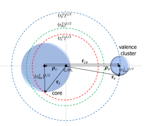
Figure 1: Coordinates of the two-body structure of the halo nucleus and for details refer to the main text.

The mean distance from the centre of the core to the valence neutron(s) in one- and two-neutron halo nuclei, $r_{cv}^{rms}$, can be determined from the charge radius, the matter radius, and the $B(E1)$ value from the Coulomb dissociation measurement, respectively, as illustrated in Eq. (16) [2].

Consider a halo nucleus with mass number $A$, consisting of core with mass number $A_{c}$ and a cluster of valence neutrons with mass number $A_{v}$. Now we define $r_{m}$, $r_{mc}$ and $r_{mv}$ as the internal coordinates relative to their centre of mass, inside of the halo nucleus, the core and valence cluster in free space, respectively. This allows us to extract the corresponding r.m.s. mass radii $r^{rms}_{m}$, $r^{rms}_{mc}$ and $r^{rms}_{mv}$, by weighing with the associated matter distributions (as illustrated in Fig. 1). Inside the halo nucleus, the core and the valence cluster are displaced from their common centre of mass by the vectors ${\bf\it\rho}_{c}$ and ${\bf\it\rho}_{v}$ with $A_{v}{\bf\it\rho}_{v}=-A_{c}{\bf\it\rho}_{c}$, so that we find the radii around this common centre of mass as

$$\left\langle r_{i}^{2}\right\rangle = \left\langle\rho_{i}^{2}\right\rangle+\left\langle r_{mi}^{2}\right\rangle\,,$$ (6)

for $i=c,v$.

By using Eq. (6) in Eq. (8) we get

$$\rho^{rms}_{c}=\left\langle\rho_{c}^{2}\right\rangle^{1/2}=\sqrt{\frac{A_{v}}{A_{c}A}\left(A\left\langle r_{m}^{2}\right\rangle-A_{c}\left\langle r_{mc}^{2}\right\rangle-A_{v}\left\langle r_{mv}^{2}\right\rangle\right)}$$ (7)

and a similar expression for $\rho^{rms}_{v}$, which allows us to evaluate the matter radius of the halo nucleus as

$$A\left\langle r_{m}^{2}\right\rangle=A_{c}\left\langle r_{c}^{2}\right\rangle+A_{v}\left\langle r_{v}^{2}\right\rangle\,.$$ (8)

Combining these equations, using ${\bf\it r}_{cv}=-{\bf\it\rho}_{c}+{\bf\it\rho}_{v}$, the distance between the core and valence cluster is given by

$$r^{rms}_{cv}=\sqrt{\frac{A}{A_{c}A_{v}}\left(A\left\langle r_{m}^{2}\right\rangle-A_{c}\left\langle r_{mc}^{2}\right\rangle-A_{v}\left\langle r_{mv}^{2}\right\rangle\right)}$$ (9)

For a one-neutron halo nuclei, we use $r_{mv}$ as the nucleon radius of about 1 fm.

For two-neutron halo nuclei as a two-body structure, we can not determine the r.m.s. radius of the cluster of the two neutrons as one body, so we can use an approximate value of $2$ fm as a double of the radius of one neutron using the sphere packing principle.

The r.m.s. matter radii can be extracted from the measurement of reaction cross sections at intermediate to high energies using a Glauber model [58, 2]. They can also be obtained from high-energy elastic proton scattering [2].

II.3 Dipole strength distributions

The reduced transition probability for an $E\lambda$ excitation between two states is normally presented as [59, 60]

$$B\left(E\lambda;\ \ell_{0}j_{0}J_{0}\rightarrow ljJ\right)=C_{0}^{2\lambda}\frac{\left|\left\langle\ell jJ\left\|\mathcal{O}_{E\lambda}\right\|\ell_{0}j_{0}J_{0}\right\rangle\right|^{2}}{2J_{0}+1}.$$ (10)

Here $\ket{\ell_{0}j_{0}J_{0}}$ represents the ground state and $\ket{\ell jJ}$ stands for states with total angular momentum $J$ (for continuum states we label it with continuum energy $\varepsilon$ and momentum $\hbar k$). The quantity $\mathcal{O}_{E\lambda}$ is the electric multipole operator of order $\lambda$ and is given by $Z_{\rm eff}^{(\lambda)}r^{\lambda}Y_{\lambda\mu}\left(\hat{\bm{r}}\right)$, where we take the effective charge of the form

$$Z_{\rm eff}^{(\lambda)}e=Z_{v}e\left(-\frac{A_{c}}{A}\right)^{\lambda}+Z_{c}e\left(\frac{A_{v}}{A}\right)^{\lambda}$$ (11)

where $Z,A$, $Z_{c},A_{c}$ and $Z_{v}.A_{v}$ are the charge and mass number of the nucleus, the core and valence nucleon(s), respectively.

For the electromagnetic breakup of the nucleus into the core and cluster of valence nucleon(s) with relative energy $\varepsilon$ and momentum $\hbar k$, the reduced transition probability can be given by summation over all possible angular momentum states of the continuum as [60]

$$\frac{dB}{d\varepsilon}\left(E\lambda;\ \ell_{0}j_{0}J_{0}\rightarrow k\ell jJ\right) =\frac{C_{0}^{2\lambda}\mu k}{(2\pi)^{3}\hbar^{2}}$$

$$\sum_{\ell,j,I_{c},J}\frac{\left|\left\langle k\ell jJ\left\|\mathcal{O}_{E\lambda}\right\|\ell_{0}j_{0}J_{0}\right\rangle\right|^{2}}{2J_{0}+1}.$$ (12)

The initial and final radial wave functions $u_{l_{0}j_{0}}^{J_{0}}$ and $u_{\varepsilon lj}^{J}$ do not depend on the angular momentum $j$ and $J$ and for the summation over all possible $j$ and $J$, Eq.(II.3) can be reduced to

$$\frac{dB(E\lambda)}{d\varepsilon} = C_{0}^{2\lambda}\frac{(2\lambda+1)}{4\pi}(Z_{\rm eff}^{(\lambda)}e)^{2}\sum_{l}\langle\ell_{0}0\lambda 0|\ell 0\rangle^{2}$$ (13)

$$\times\Bigg{|}\int_{0}^{\infty}dr\ r^{\lambda}\ u_{\varepsilon\ell j}^{J}\left(r\right)\ u_{\ell_{0}j_{0}}^{J_{0}}\left(r\right)\Bigg{|}^{2}.$$

We use the asymptotic expansion of the radial wave function, i.e., plane waves expanded in terms of spherical Bessel functions. Thus, Eq. (13) gives us the low-lying multipole strength distribution for the valence neutron(s) in weakly bound systems.

To include the different spins of the core, the initial bound wave function is given as a linear combination of these different core spins with valence nucleon(s) spin [61]

$$|J_{0}M_{0}\rangle=\sum_{n_{0}\ell_{0}j_{0}}\alpha(I_{c}^{\pi},n_{0}\ell_{0}j_{0})|I_{c}^{\pi}\otimes n\ell_{0}j_{0}\rangle$$ (14)

in which the summation over the weights or the square of spectroscopic amplitudes, $\sum_{n_{0}\ell_{0}j_{0}}[\alpha(I_{c}^{\pi},n_{0}\ell_{0}j_{0})]^{2}$ is unity, and then Eq. (13) becomes

$$\frac{dB(E\lambda)}{d\varepsilon}= C_{0}^{2\lambda}\frac{(2\lambda+1)}{4\pi}(Z_{\rm eff}^{(\lambda)}e)^{2}\sum_{n_{0}\ell_{0}j_{0}}[\alpha(I_{c}^{\pi},n_{0}\ell_{0}j_{0})]^{2}$$

$$\sum_{\ell}\langle\ell_{0}0\lambda 0|\ell 0\rangle^{2}\ \Bigg{|}\int_{0}^{\infty}dr\ r^{\lambda}\ u_{\varepsilon\ell j}^{J}\left(r\right)\ u_{\ell_{0}j_{0}}^{J_{0}}\left(r\right)\Bigg{|}^{2}.$$ (15)

The total strength for an $E\lambda$ transition from a bound state to all possible final states is given by

$$B(E1)=\int_{0}^{\infty}\frac{dB(E1)}{d\varepsilon}d\varepsilon=\frac{3}{4\pi}(Z_{\rm eff}^{(1)}e)^{2}\left\langle r_{cv}^{2}\right\rangle\,.$$ (16)

The soft dipole mode (SDM) satisfies an energy-weighted sum rule (EWSR) which is evaluated as [12]

$$S_{1}=\int_{0}^{\infty}(\varepsilon_{0}+\varepsilon)\frac{dB(E1)}{d\varepsilon}d\varepsilon\,.$$ (17)

If the transition is purely single-paricle, this sum evaluates to [52, 12]

$$S_{1}=\frac{9}{4\pi}\frac{\hbar^{2}e^{2}}{2m}\left(\frac{NZ}{A}-\frac{N_{c}Z_{c}}{A_{c}}\right)\,,$$ (18)

where $N$ and $N_{c}$ are the neutron number of the nucleus and its core, respectively. The ratio between the observed sum Eq. (17) and the cluster sum Eq. (18) can also be used to extract the spectroscopic factor for the halo state [12].

III Results and discussions

Table 1: The combinations of the core spin-parity ($I^{\pi}_{c})$ with $0s$ and $0d$ valence cluster orbits for the ground state of different halo nuclei.

System	System	core	valence orbit
core$+1n/2n$	$J^{\pi}$	$I_{c}^{\pi}$	$nl$
10Be$+n$	$1/2^{+}$	$0^{+}$	$0s$
	$1/2^{+}$	$2^{+}$	$0d$
14C$+n$	$1/2^{+}$	$0^{+}$	$0s$
	$1/2^{+}$	$2^{+}$	$0d$
4He$+2n$	$0^{+}$	$0^{+}$	$0s$, $0d$
9Li$+2n$	$3/2^{-}$	$3/2^{-}$	$0s,0d$

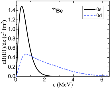
Figure 2: Dipole strength distribution $dB(E1)/d\varepsilon$ for two different choices of the ground state for ¹¹Be.

We apply the formalism to two 1$n$-halo nuclei (¹¹Be and ¹⁵C) and two 2$n$-halo nuclei (⁶He and ¹¹Li). The ground state spin and parity of ¹¹Be and ¹⁵C is $1/2^{+}$. There are two options (i) the core (¹⁰Be or ¹⁴C) has $I_{c}^{\pi}=0^{+}$ and the valence neutron is in the $0s$ orbit, or (ii) the core has $I_{c}^{\pi}=2^{+}$ and the valence neutron is in $0d$ orbit. In the case of $2n$ halos ⁶He and ¹¹Li, both core and halo nucleus have the same angular momentum, $0^{+}$ and $3/2^{-}$, respectively. Thus the two neutrons in the valence cluster must be coupled to angular momentum zero ($0^{+}$), which is compatible with two $0s$ or $0d$ single particle states.

Table 1 summarizes the potential ground states for these nuclei. By combining $0s$ and $0d$ orbits, as expressed in Eq. (II.3) with the constraint that the summation over spectroscopic weights is unity, we expect different spectroscopic weights.

Table 2: The distance between the core and valence neutron(s) ($r^{rms}_{cv}$) for different nuclei.

System	$r^{rms}_{mc}$	$r^{rms}_{m}$	$r^{rms}_{cv}$ Eq.(9)
core$+1n/2n$	fm	fm	fm
10Be+$n$	2.39 [38]	2.90 [62]	6.15
14C+$n$	2.43 [63]	2.60 [63]	4.36
4He+$2n$	1.57 [64]	2.48 [64]	3.78
9Li+$2n$	2.53 [65]	3.10 [64]	4.94

Here, it is worth noting that in the absence of spin-orbit splitting, the computed $dB(E\lambda)/d\varepsilon$ values for $0d_{3/2}$ and $0d_{5/2}$ orbitals are identical. Consequently, we treat the $0d$ orbit of the neutron(s) in the ground state as a single entity. We also note that $s$-states give rise to a low-energy peak in $dB(E\lambda)/d\varepsilon$, but $d$-states give a long tail, which explains why we need a combination of these two. This can be seen in Fig. 2 for the case of ¹¹Be. All the calculations shown in Fig. 2 have the same integrated $B(E1)$ value and identical $r_{cv}^{rms}$.

Table 3: Results for the integrated $B(E1)$ (non-energy weighted), the core-valence radius $r_{cv}^{rms}$, and sum rule $S_{1}$ for one and two-neutron halo nuclei. The first five columns detail the system structure information, the value of $R_{0}$, the computed value of $C_{0}^{2}$, and the probabilities assigned to the $0s$ and $0d$ states. The remaining columns compare our calculations with experimental results and the sum rule values.

System	$R_{0}$ (fm)	$C_{0}^{2}$	weight $\alpha^{2}$		$B(E1)$ ($e^{2}$fm2)		$r_{cv}^{rms}$ (fm)		$S_{1}$ ($e^{2}$fm2)
			$0s$	$0d$	Calc.	exp.	Calc.	exp.	Calc.	Eq.(18)
10Be+$n$	11.72	0.28	0.46	0.54	1.19	0.90(6)[11], 1.3(3)[10], 1.05(6)[12]	6.15	6.4(7)[10], 5.7(4)[11], 5.77(16), 6.1(5) [12]	2.21	2.18
14C+$n$	7.43	0.34	0.80	0.20	0.73	0.53(5), 0.77(7) [13]	4.36	4.5(2) [13]	2.46	2.55
4He+$2n$	5.42	0.55	0.37	0.63	1.53	1.2(2) [4], 1.6(2) [6]	3.79	3.36(39)[4], 3.9(2)[6]	8.81	4.95
9Li+$2n$	9.84	0.25	0.30	0.70	1.73	1.78(22) [9]	4.94	5.01(32) [9], 6.2(5) [66]	2.82	2.70

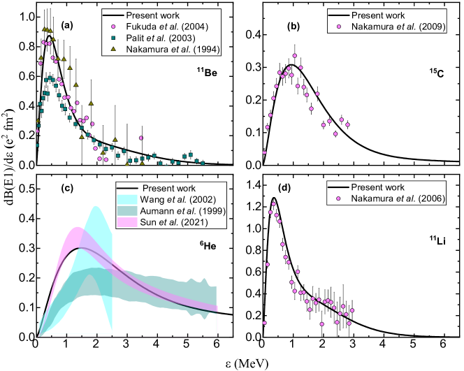
Figure 3: Dipole strength distribution $dB(E1)/d\varepsilon$ for one and two-neutron halo nuclei. The solid line represents the calculations using a combination of $0s$ and $0d$-orbits; refer to Table 3 for detailed information on these combinations. The calculated $dB(E1)/d\varepsilon$ are compared with the experimental data. (a) shows ¹¹B and data from Nakamura et al. at $72$ MeV/A [10], Palit et al. at $520$ MeV/A [11], and Fukuda et al. at $69$ MeV/A [12]; (b) shows ¹⁵C and data from Nakamura et al. at $68$ MeV/A [13]; (c) gives results for ⁶He with data from Aumann et al. at $240$ MeV/A [4], Wang et al. at $23.9$ MeV/A [67], and Sun et al. at $70$ MeV/A [6]; (d) shows ¹¹Li with data from Nakamura et al. at $70$ MeV/A [9].

Determining $r_{cv}^{rms}$ values for the calculation of $C_{0}$ via Eq. (5) is straightforward using Eq. (9). The inputs of Eq. (9) and the obtained values of $r^{rms}_{cv}$ are listed in Table 2. For instance, using the r.m.s. radii of ¹¹Be and ¹⁰Be yields $r^{rms}_{cv}$ as $6.15$ fm. A similar procedure for ¹⁵C gives $r_{cv}=4.36$ fm. For the ⁶He and ¹¹Li nuclei we get 3.78 and 4.94 fm respectively. It is clear that the obtained $r^{rms}_{cv}$ are in good agreement with those extracted from the experimental $B(E1)$ values as listed in table 3.

In our framework, the calculation of $dB(E1)/d\varepsilon$ involves utilizing Eq. (II.3), where we search for spectroscopic factors $A^{2}$ for both $s$- and $d$-states that best fit the experimental data. This allows us to compare our calculated integrated $B(E1)$ values with the experimental ones, as outlined in Table 3. The extracted value of $R_{0}$ depends on the separation energy $\varepsilon_{0}$, see Eq. (4). For ⁶He, we use a one-neutron separation energy of $\varepsilon_{0}=s_{n}=1.71$ MeV instead of the original reference value $\varepsilon_{0}=s_{2n}=0.975$ MeV, which is close to the $1.6$ MeV corrected value suggested by Moro et al [49]. Similarly, for ¹¹Li, we use $\varepsilon_{0}=s_{n}=0.396$ MeV. Initially, we explored combinations involving $1s$ and $0d$ states but found inadequate agreement with the data. However, employing a combination of $0s$ and $0d$ across all nuclei yields better results. The calculated $dB(E1)/d\varepsilon$ for various one and two-neutron nuclei are shown in Fig. 3, with the corresponding integrated $B(E1)$ values and $r_{cv}$ listed in Table 3.

Remarkably, the $0s$ and $0d$ state combinations consistently provide excellent agreements with experimental data across all nuclei. Furthermore, the extracted $B(E1)$ and $r_{cv}$ values closely match the experimental data. Moreover, the calculated $S_{1}$ from $dB(E1)/d\varepsilon$ aligns well with the theoretical cluster sum rule values described by Eq.(18).

Our calculations for the nuclei ¹¹Be, ¹⁵C, ⁶He, and ¹¹Li shown in panels (a), (b), (c), and (d) respectively, of Fig. 3, yield excellent results that agree well with the experimental data. Specifically, for ¹¹Be our model adequately captures the average of available $dB(E1)/d\varepsilon$ data [10, 11, 12]. The resulting $B(E1)$ and $r_{v}$ values align closely with experimental observations. Despite variations in extracted $S_{1}$ values, our model consistently produces values near the total cluster sum rule, affirming its robustness. Similarly, for ¹⁵C, our approach agrees well with the experimental data, with calculated $S_{1}$ values mirroring theoretical cluster sums. In ⁶He, our model accurately reproduces the peak position at 1.4 MeV and shape of $dB(E1)/d\varepsilon$ of the data [6], with integrated $B(E1)$ strength and $r_{v}$ in line with experimental findings, demonstrating good agreement with previous results. Lastly, in ¹¹Li, we find favourable fits to data, with integrated $B(E1)$ and $R_{v}$ values consistent with experimental reports, and $S_{1}$ values aligning well with theoretical cluster sums. These consistent successes across multiple nuclei underscore the efficacy and reliability of our model.

IV Summary and conclusion

In summary, a simple cluster shell-model approximation is presented to estimate the ground state wave function of halo nuclei and applied successfully to reproduce the soft $E1$ response function distribution for the 1$n$-halo nuclei ¹¹Be and ¹⁵C and 2$n$-halo nuclei ⁶He and ¹¹Li. This is a very powerful and surprising result, in light of the very simple wavefunctions and the equally simple operator renormalisation used. However, with only a single free parameter, the $sd$ mixing, we are able to give a very good quantitative description of the experimental results. Also, a new simplified expression for the distance between the two clusters of halo nuclei is presented. In general, this expression can be helpful in determining the distance between two clusters within a nucleus, for example $\alpha+t$ structure of ${}^{7}Li$ and $\alpha+d$ structure of ${}^{6}Li$, using the r.m.s. radius of the nucleus and its clusters as free nuclei. In the future, we hope to give a better foundation for the operator renormalisation used. We also intend to see whether a similar argument can be used effectively for heavier nuclei and at the proton dripline.

References

- Nowacki et al. [2021] F. Nowacki, A. Obertelli, and A. Poves, Prog. Part. Nucl. Phys. 120, 103866 (2021).
- Tanihata et al. [2013] I. Tanihata, H. Savajols, and R. Kanungo, Prog. Part. Nucl. Phys. 68, 215 (2013).
- Diaz-Torres and Heinz [2024] A. Diaz-Torres and S. Heinz, Europhysics News 55, 26 (2024).
- Aumann et al. [1999] T. Aumann, D. Aleksandrov, L. Axelsson, T. Baumann, M. J. G. Borge, L. V. Chulkov, J. Cub, W. Dostal, B. Eberlein, T. W. Elze, H. Emling, H. Geissel, V. Z. Goldberg, M. Golovkov, A. Grünschloß, M. Hellström, K. Hencken, J. Holeczek, R. Holzmann, B. Jonson, A. A. Korshenninikov, J. V. Kratz, G. Kraus, R. Kulessa, Y. Leifels, A. Leistenschneider, T. Leth, I. Mukha, G. Münzenberg, F. Nickel, T. Nilsson, G. Nyman, B. Petersen, M. Pfützner, A. Richter, K. Riisager, C. Scheidenberger, G. Schrieder, W. Schwab, H. Simon, M. H. Smedberg, M. Steiner, J. Stroth, A. Surowiec, T. Suzuki, O. Tengblad, and M. V. Zhukov, Phys. Rev. C 59, 1252 (1999).
- Meister et al. [2002] M. Meister, K. Markenroth, D. Aleksandrov, T. Aumann, T. Baumann, M. J. G. Borge, L. V. Chulkov, D. Cortina-Gil, B. Eberlein, T. W. Elze, H. Emling, H. Geissel, M. Hellström, B. Jonson, J. V. Kratz, R. Kulessa, A. Leistenschneider, I. Mukha, G. Münzenberg, F. Nickel, T. Nilsson, G. Nyman, M. Pfützner, V. Pribora, A. Richter, K. Riisager, C. Scheidenberger, G. Schrieder, H. Simon, O. Tengblad, and M. V. Zhukov, Nucl. Phys. A 700, 3 (2002).
- Sun et al. [2021] Y. L. Sun, T. Nakamura, Y. Kondo, Y. Satou, J. Lee, T. Matsumoto, K. Ogata, Y. Kikuchi, N. Aoi, Y. Ichikawa, K. Ieki, M. Ishihara, T. Kobayshi, T. Motobayashi, H. Otsu, H. Sakurai, T. Shimamura, S. Shimoura, T. Shinohara, T. Sugimoto, S. Takeuchi, Y. Togano, and K. Yoneda, Phys. Lett. B 814, 136072 (2021).
- Fortunato et al. [2014] L. Fortunato, R. Chatterjee, J. Singh, and A. Vitturi, Phys. Rev. C 90, 064301 (2014).
- Singh et al. [2016a] J. Singh, L. Fortunato, A. Vitturi, and R. Chatterjee, Eur. Phys. J. A 52, 209 (2016a).
- Nakamura et al. [2006] T. Nakamura, A. M. Vinodkumar, T. Sugimoto, N. Aoi, H. Baba, D. Bazin, N. Fukuda, T. Gomi, H. Hasegawa, N. Imai, M. Ishihara, T. Kobayashi, Y. Kondo, T. Kubo, M. Miura, T. Motobayashi, H. Otsu, A. Saito, H. Sakurai, S. Shimoura, K. Watanabe, Y. X. Watanabe, T. Yakushiji, Y. Yanagisawa, and K. Yoneda, Phys. Rev. Lett. 96, 252502 (2006).
- Nakamura et al. [1994] T. Nakamura, S. Shimoura, T. Kobayashi, T. Teranishi, K. Abe, N. Aoi, Y. Doki, M. Fujimaki, N. Inabe, N. Iwasa, K. Katori, T. Kubo, H. Okuno, T. Suzuki, I. Tanihata, Y. Watanabe, A. Yoshida, and M. Ishihara, Phys. Lett. B 331, 296 (1994).
- Palit et al. [2003] R. Palit, P. Adrich, T. Aumann, K. Boretzky, B. V. Carlson, D. Cortina, U. Datta Pramanik, T. W. Elze, H. Emling, H. Geissel, M. Hellström, K. L. Jones, J. V. Kratz, R. Kulessa, Y. Leifels, A. Leistenschneider, G. Münzenberg, C. Nociforo, P. Reiter, H. Simon, K. Sümmerer, and W. Walus (LAND/FRS Collaboration), Phys. Rev. C 68, 034318 (2003).
- Fukuda et al. [2004] N. Fukuda, T. Nakamura, N. Aoi, N. Imai, M. Ishihara, T. Kobayashi, H. Iwasaki, T. Kubo, A. Mengoni, M. Notani, H. Otsu, H. Sakurai, S. Shimoura, T. Teranishi, Y. X. Watanabe, and K. Yoneda, Phys. Rev. C 70, 054606 (2004).
- Nakamura et al. [2009] T. Nakamura, N. Fukuda, N. Aoi, N. Imai, M. Ishihara, H. Iwasaki, T. Kobayashi, T. Kubo, A. Mengoni, T. Motobayashi, M. Notani, H. Otsu, H. Sakurai, S. Shimoura, T. Teranishi, Y. X. Watanabe, and K. Yoneda, Phys. Rev. C 79, 035805 (2009).
- Suzuki et al. [2002] T. Suzuki, Y. Ogawa, M. Chiba, M. Fukuda, N. Iwasa, T. Izumikawa, R. Kanungo, Y. Kawamura, A. Ozawa, T. Suda, I. Tanihata, S. Watanabe, T. Yamaguchi, and Y. Yamaguchi, Phys. Rev. Lett. 89, 012501 (2002).
- Cook et al. [2020] K. J. Cook, T. Nakamura, Y. Kondo, K. Hagino, K. Ogata, A. T. Saito, N. L. Achouri, T. Aumann, H. Baba, F. Delaunay, Q. Deshayes, P. Doornenbal, N. Fukuda, J. Gibelin, J. W. Hwang, N. Inabe, T. Isobe, D. Kameda, D. Kanno, S. Kim, N. Kobayashi, T. Kobayashi, T. Kubo, S. Leblond, J. Lee, F. M. Marqués, R. Minakata, T. Motobayashi, K. Muto, T. Murakami, D. Murai, T. Nakashima, N. Nakatsuka, A. Navin, S. Nishi, S. Ogoshi, N. A. Orr, H. Otsu, H. Sato, Y. Satou, Y. Shimizu, H. Suzuki, K. Takahashi, H. Takeda, S. Takeuchi, R. Tanaka, Y. Togano, J. Tsubota, A. G. Tuff, M. Vandebrouck, and K. Yoneda, Phys. Rev. Lett. 124, 212503 (2020).
- Tanaka et al. [2010] K. Tanaka, T. Yamaguchi, T. Suzuki, T. Ohtsubo, M. Fukuda, D. Nishimura, M. Takechi, K. Ogata, A. Ozawa, T. Izumikawa, T. Aiba, N. Aoi, H. Baba, Y. Hashizume, K. Inafuku, N. Iwasa, K. Kobayashi, M. Komuro, Y. Kondo, T. Kubo, M. Kurokawa, T. Matsuyama, S. Michimasa, T. Motobayashi, T. Nakabayashi, S. Nakajima, T. Nakamura, H. Sakurai, R. Shinoda, M. Shinohara, H. Suzuki, E. Takeshita, S. Takeuchi, Y. Togano, K. Yamada, T. Yasuno, and M. Yoshitake, Phys. Rev. Lett. 104, 062701 (2010).
- Togano et al. [2016] Y. Togano, T. Nakamura, Y. Kondo, J. A. Tostevin, A. T. Saito, J. Gibelin, N. A. Orr, N. L. Achouri, T. Aumann, H. Baba, F. Delaunay, P. Doornenbal, N. Fukuda, J. W. Hwang, N. Inabe, T. Isobe, D. Kameda, D. Kanno, S. Kim, N. Kobayashi, T. Kobayashi, T. Kubo, S. Leblond, J. Lee, F. M. Marqués, R. Minakata, T. Motobayashi, D. Murai, T. Murakami, K. Muto, T. Nakashima, N. Nakatsuka, A. Navin, S. Nishi, S. Ogoshi, H. Otsu, H. Sato, Y. Satou, Y. Shimizu, H. Suzuki, K. Takahashi, H. Takeda, S. Takeuchi, R. Tanaka, A. G. Tuff, M. Vandebrouck, and K. Yoneda, Phys. Lett. B 761, 412 (2016).
- Singh et al. [2019] J. Singh, W. Horiuchi, L. Fortunato, and A. Vitturi, Few-Body Syst. 60, 50 (2019).
- Bagchi et al. [2020] S. Bagchi, R. Kanungo, Y. K. Tanaka, H. Geissel, P. Doornenbal, W. Horiuchi, G. Hagen, T. Suzuki, N. Tsunoda, D. S. Ahn, H. Baba, K. Behr, F. Browne, S. Chen, M. L. Cortés, A. Estradé, N. Fukuda, M. Holl, K. Itahashi, N. Iwasa, G. R. Jansen, W. G. Jiang, S. Kaur, A. O. Macchiavelli, S. Y. Matsumoto, S. Momiyama, I. Murray, T. Nakamura, S. J. Novario, H. J. Ong, T. Otsuka, T. Papenbrock, S. Paschalis, A. Prochazka, C. Scheidenberger, P. Schrock, Y. Shimizu, D. Steppenbeck, H. Sakurai, D. Suzuki, H. Suzuki, M. Takechi, H. Takeda, S. Takeuchi, R. Taniuchi, K. Wimmer, and K. Yoshida, Phys. Rev. Lett. 124, 222504 (2020).
- Singh et al. [2020] J. Singh, J. Casal, W. Horiuchi, L. Fortunato, and A. Vitturi, Phys. Rev. C 101, 024310 (2020).
- Fortunato et al. [2020] L. Fortunato, J. Casal, W. Horiuchi, J. Singh, and A. Vitturi, Commun. Phys. 3, 132 (2020).
- Casal et al. [2020] J. Casal, J. Singh, L. Fortunato, W. Horiuchi, and A. Vitturi, Phys. Rev. C 102, 064627 (2020).
- Kobayashi et al. [2014] N. Kobayashi, T. Nakamura, Y. Kondo, J. A. Tostevin, Y. Utsuno, N. Aoi, H. Baba, R. Barthelemy, M. A. Famiano, N. Fukuda, N. Inabe, M. Ishihara, R. Kanungo, S. Kim, T. Kubo, G. S. Lee, H. S. Lee, M. Matsushita, T. Motobayashi, T. Ohnishi, N. A. Orr, H. Otsu, T. Otsuka, T. Sako, H. Sakurai, Y. Satou, T. Sumikama, H. Takeda, S. Takeuchi, R. Tanaka, Y. Togano, and K. Yoneda, Phys. Rev. Lett. 112, 242501 (2014).
- Manju et al. [2021] Manju, M. Dan, G. Singh, J. Singh, Shubhchintak, and R. Chatterjee, Nucl. Phys. A 1010, 122194 (2021).
- Masui et al. [2020] H. Masui, W. Horiuchi, and M. Kimura, Phys. Rev. C 101, 041303 (2020).
- Singh et al. [2022] G. Singh, J. Singh, J. Casal, and L. Fortunato, Phys. Rev. C 105, 014328 (2022).
- Singh et al. [2016b] G. Singh, Shubhchintak, and R. Chatterjee, Phys. Rev. C 94, 024606 (2016b).
- Zhang et al. [2023a] K. Y. Zhang, P. Papakonstantinou, M.-H. Mun, Y. Kim, H. Yan, and X.-X. Sun, Phys. Rev. C 107, L041303 (2023a).
- Singh et al. [2024] J. Singh, J. Casal, W. Horiuchi, N. R. Walet, and W. Satuła, Phys. Lett. B 853, 138694 (2024).
- Zhang et al. [2023b] K. Y. Zhang, S. Q. Zhang, and J. Meng, Phys. Rev. C 108, L041301 (2023b).
- Li et al. [2024] H. H. Li, J. G. Li, M. R. Xie, and W. Zuo, Phys. Rev. C 109, L061304 (2024).
- Hove et al. [2018] D. Hove, E. Garrido, P. Sarriguren, D. V. Fedorov, H. O. U. Fynbo, A. S. Jensen, and N. T. Zinner, Phys. Rev. Lett. 120, 052502 (2018).
- Horiuchi et al. [2022] W. Horiuchi, Y. Suzuki, M. A. Shalchi, and L. Tomio, Phys. Rev. C 105, 024310 (2022).
- Hansen and Jonson [1987] P. G. Hansen and B. Jonson, Europhys. Lett. 4, 409 (1987).
- Zhukov et al. [1993] M. V. Zhukov, B. V. Danilin, D. V. Fedorov, J. M. Bang, I. J. Thompson, and J. S. Vaagen, Phys. Rep. 231, 151 (1993).
- Hagino and Sagawa [2005] K. Hagino and H. Sagawa, Phys. Rev. C 72, 044321 (2005).
- Kikuchi et al. [2016] Y. Kikuchi, K. Ogata, Y. Kubota, M. Sasano, and T. Uesaka, Prog. Theor. Exp. Phys. 2016, 103D03 (2016).
- Tanihata et al. [1985] I. Tanihata, H. Hamagaki, O. Hashimoto, Y. Shida, N. Yoshikawa, K. Sugimoto, O. Yamakawa, T. Kobayashi, and N. Takahashi, Phys. Rev. Lett. 55, 2676 (1985).
- Aumann and Nakamura [2013] T. Aumann and T. Nakamura, Physica Scripta 2013, 014012 (2013).
- Aumann [2019] T. Aumann, Eur. Phys. J. A 55, 234 (2019).
- Chatterjee and Shyam [2018] R. Chatterjee and R. Shyam, Prog. Part. Nucl. Phys. 103, 67 (2018).
- Moschini and Capel [2019] L. Moschini and P. Capel, Phys. Lett. B 790, 367 (2019).
- Singh et al. [2021] J. Singh, T. Matsumoto, and K. Ogata, Prog. Theor. Exp. Phys. 2021, 073D01 (2021).
- Matsumoto et al. [2004] T. Matsumoto, E. Hiyama, K. Ogata, Y. Iseri, M. Kamimura, S. Chiba, and M. Yahiro, Phys. Rev. C 70, 061601(R) (2004).
- Casal et al. [2013] J. Casal, M. Rodríguez-Gallardo, and J. M. Arias, Phys. Rev. C 88, 014327 (2013).
- Sagawa and Hagino [2015] H. Sagawa and K. Hagino, Eur. Phys. J. A 51, 102 (2015).
- Singh et al. [2016c] J. Singh, L. Fortunato, A. Vitturi, and R. Chatterjee, Eur. Phys. J. A 52, 209 (2016c).
- Horiuchi and Suzuki [2006] W. Horiuchi and Y. Suzuki, Phys. Rev. C 74, 034311 (2006).
- Moro et al. [2007] A. M. Moro, K. Rusek, J. M. Arias, J. Gómez-Camacho, and M. Rodríguez-Gallardo, Phys. Rev. C 75, 064607 (2007).
- Suzuki and Ikeda [1988] Y. Suzuki and K. Ikeda, Phys. Rev. C 38, 410 (1988).
- Suzuki and Ju [1990] Y. Suzuki and W. J. Ju, Phys. Rev. C 41, 736 (1990).
- Suzuki [1991] Y. Suzuki, Nucl. Phys. A 528, 395 (1991).
- Korsheninnikov et al. [1997] A. A. Korsheninnikov, E. A. Kuzmin, E. Y. Nikolskii, C. A. Bertulani, O. V. Bochkarev, S. Fukuda, T. Kobayashi, S. Momota, B. G. Novatskii, A. A. Ogloblin, A. Ozawa, V. Pribora, I. Tanihata, and K. Yoshida, Nucl. Phys. A 616, 189 (1997), radioactive Nuclear Beams.
- Brody et al. [1960] T. A. Brody, G. Jacob, and M. Moshinsky, Nucl. Phys. 17, 16 (1960).
- Goldhammer [1963] P. Goldhammer, Rev. Mod. Phys. 35, 40 (1963).
- Moshinsky [1969] M. Moshinsky, The harmonic oscillator in modern physics: from atoms to quarks (Gordon Press, New York, 1969).
- Talmi [1993] I. Talmi, Simple Models of Complex Nuclei (1st ed.) (Routledge, 1993).
- Ozawa et al. [2001] A. Ozawa, T. Suzuki, and I. Tanihata, Nucl. Phys. A 693, 32 (2001), radioactive Nuclear Beams.
- Typel and Baur [2005] S. Typel and G. Baur, Nucl. Phys. A 759, 247 (2005).
- Bertulani [2003] C. A. Bertulani, Comput. Phys. Commun. 156, 123 (2003).
- Nakamura [2023] T. Nakamura, in Handbook of Nuclear Physics, edited by I. Tanihata, H. Toki, and T. Kajino (Springer Nature Singapore, Singapore, 2023) pp. 1205–1241.
- Al-Khalili et al. [1996] J. S. Al-Khalili, J. A. Tostevin, and I. J. Thompson, Phys. Rev. C 54, 1843 (1996).
- Dobrovolsky et al. [2021] A. V. Dobrovolsky, G. A. Korolev, S. Tang, G. D. Alkhazov, G. Colò, I. Dillmann, P. Egelhof, A. Estradé, F. Farinon, H. Geissel, S. Ilieva, A. G. Inglessi, Y. Ke, A. V. Khanzadeev, O. A. Kiselev, J. Kurcewicz, L. X. Chung, Y. A. Litvinov, G. E. Petrov, A. Prochazka, C. Scheidenberger, L. O. Sergeev, H. Simon, M. Takechi, V. Volkov, A. A. Vorobyov, H. Weick, and V. I. Yatsoura, Nucl. Phys. A 1008, 122154 (2021).
- Tanihata et al. [1988] I. Tanihata, T. Kobayashi, O. Yamakawa, S. Shimoura, K. Ekuni, K. Sugimoto, N. Takahashi, T. Shimoda, and H. Sato, Phys. Lett. B 206, 592 (1988).
- Liatard et al. [1990] E. Liatard, J. F. Bruandet, F. Glasser, S. Kox, T. U. Chan, G. J. Costa, C. Heitz, Y. E. Masri, F. Hanappe, R. Bimbot, D. Guillemaud-Mueller, and A. C. Mueller, Europhys. Lett. 13, 401 (1990).
- Sánchez et al. [2006] R. Sánchez, W. Nörtershäuser, G. Ewald, D. Albers, J. Behr, P. Bricault, B. A. Bushaw, A. Dax, J. Dilling, M. Dombsky, G. W. F. Drake, S. Götte, R. Kirchner, H.-J. Kluge, T. Kühl, J. Lassen, C. D. P. Levy, M. R. Pearson, E. J. Prime, V. Ryjkov, A. Wojtaszek, Z.-C. Yan, and C. Zimmermann, Phys. Rev. Lett. 96, 033002 (2006).
- Wang et al. [2002] J. Wang, A. Galonsky, J. J. Kruse, E. Tryggestad, R. H. White-Stevens, P. D. Zecher, Y. Iwata, K. Ieki, A. Horváth, F. Deák, A. Kiss, Z. Seres, J. J. Kolata, J. von Schwarzenberg, R. E. Warner, and H. Schelin, Phys. Rev. C 65, 034306 (2002).