Insights from Large-Scale Communications: Initiation

Abstract

This paper offers an original theoretical framework to quantify the information content associated with cosmological structure formation. The formalism is developed and employed to study the spectrum of information underlying the galaxy distribution in the observable Universe. Using data from SDSS DR18 we further quantify the information sharing across different parts of the studied volume. An attempt to validate the assumption of cosmic homogeneity is made, which rules out the presence of a Universal scale of uniformity below $130{\,h^{-1}\,{\rm Mpc}}$. In addition, an analytical study is carried out to track back the evolution of global information content up to $z=20$, where a log-normal density distribution with redshift-dependent variance, skewness, and kurtosis is used to mimic the observable Universe. A staggering $8\times 10^{144}TB$ of information loss is estimated, caused by the formation of large-scale structures in the present universe. We further illustrate how the global information budget is impacted at different epochs by the interaction between the expansion rate and growth rate of structure, taking the $\Lambda CDM$ model into account. It is found that while the growth rate of the global information content is slowing down, information loss is increasing dramatically despite an ongoing accelerated expansion.

1 Introduction

The study of galaxy clustering is the cornerstone of modern cosmology. Over the years, it has played an important role in explaining the dynamics of the Universe. peebles73 (45) introduced the primary statistical tools to characterise and quantify the properties of galaxy clustering. Later on, several seminal studies efstathiou79 (19, 26, 16, 4, 30, 10, 23, 33, 5) refined our understanding of galaxy clustering and its manifestation across different length scales. Both observational facilities and theoretical frameworks have experienced substantial advancements in the last few decades. Large-scale surveys such as the SDSS york00 (59), 2MASS skrutskie06 (53), GAMA driver11 (18) and DES abbott18 (2) have not only expanded our observational capabilities in terms of individual object detection but also has contributed in understanding the current nature and evolution of galaxy clustering in the Universe. Furthermore, theoretical models and cosmological simulations such as Millennium Run springel05 (55), Horizon Run kim15 (31), EAGLE schaye15 (49) and IllustrisTNG nelson18 (37) have played a crucial role in interpreting observational data and uncovering the underlying physical mechanisms which govern galaxy clustering in the Universe.

On smaller scales, thermally supported interstellar clouds of self-gravitating gas fragments into stars jeans1914 (29). In the presence of anisotropic gravitational forces, a much larger, uniformly rotating or non-rotating cold gas cloud undergoes a spheroidal collapse to become a galaxy lynden62 (35, 34, 9). On the other hand, the spherical collapse model gunn72 (22) explains how large galaxy clusters like Coma can form through the infall of baryonic matter into dark matter (DM) potential wells. However, the formation of the filament and pancake-like structures, that are prevalent in the nearby observable universe, can be explained through the mechanism of anisotropic ellipsoidal collapse dorosh64 (17, 60, 50). ostriker78 (39) finds evidence of an inside-out dynamical growth of galaxy clustering, which is thought to be originating from the bottom-up hierarchical merging of DM halos press74 (47, 11, 32, 52). Galaxies being the biased tracers of the DM halos are expected to be found in the sharpest density peaks of the DM distribution. To better understand the relationship between a galaxy, its associated DM host, and the space they occupy combined, it is necessary to comprehend the systematic evolution of the information content associated with the configuration of the large-scale structures occupying that space. Long before the galaxy’s formation, this space was characterised by a nearly uniform matter distribution. Over time, gravity forces the matter to collapse and form a bound object, now seen as the galaxy. This process also involves the accretion of additional matter from relatively under-dense surroundings and indirectly helps the under-dense structures to grow. This entire process in every step reduces the randomness of the whole system ( galaxy + surrounding ) and takes it towards a low probability state. The birth of a galaxy requires several conditions to be met; only a few among numerous alternate possibilities would lead to the emergence of the galaxy within a specific space-time span. For example, a larger DM halo nearby could have changed the evolutionary trajectory of the galaxy in terms of space and time. From an alternate point of view, the growth of under-densities due to the combined effect of gravitational drag and the expansion of the Universe creates structures characterised by the enormity of space or nothingness; This again reduces the existing uncertainty of the system. This complex flow of matter and space results in a spatial distribution of probability, and gives rise to a continuum of Information.

Building on the work of nyquist24 (38) and hartley28 (24), shannon48 (51) put in place the groundwork for quantifying the information entropy in classical systems characterised by discrete variables. This led to subsequent research on modelling information exchange within complex systems jaynes57 (28, 58). hawking76 (25) showed the limitations in information transmission from the ”hidden surface” of a black hole which led beken81 (7) to establish the universal upper bound of entropy. Through dimension reduction, the holographic principle thooft93 (1, 6, 56) demonstrates that information confined in a finite volume can be represented by information projected through its surface. Furthermore, the relation between the surface area and the upper entropic bound of information holds not just for black holes, but also for vast cosmological scales. Information entropy in inhomogeneous hosoya04 (27) and homogeneous pandey19 (42, 15, 14, 40) cosmological models has been studied extensively. Several studies validating cosmic homogeneity pandey15 (44, 41, 43) and isotropy sarkar19 (48), using information theory advocate the presence of a Universal scale of uniformity beyond $\sim 200{\,h^{-1}\,{\rm Mpc}}$. Using Fisher information tegmark97 (57) shows how to numerically estimate the accuracy at which observational data can determine cosmological parameters. carron13 (12) presents the sufficient statistics that use the Fisher matrix to measure the information content of a lognormal density distribution originating from a Gaussian initial condition. ensslin09 (21) develop the information field theory for reconstructing spatially distributed large-scale signals. pinho20 (36) quantifies the information content in cosmological probes and connects information entropy to Bayesian inference. Information theory is currently being applied extensively in astronomical data analysis, targeting a lossless recovery of the cosmological information encoded with the incoming signals. Despite this, a comprehensive information-theoretical technique to map the spatial information distribution in the Universe and quantify the amount of information going into creating large-scale structures is still lacking. In this study, we develop a tool that not only allows us to measure the effective amount of spatial information but also helps to determine the information sharing on various length scales associated with overall structure formation. Furthermore, it also aids in presenting a profit and loss statement for the information budget of the Universe.

Throughout the paper, we follow planck18 (46), and use the following set of cosmological parameters for comoving distance calculation, N-body simulation and estimation of global information entropy in $\Lambda CDM$ cosmology: $\Omega_{m}=0.315$;    $\Omega_{\Lambda}=0.685$;    $H_{0}=67.4$;    $\sigma_{8}=0.811$.

2 Method of Analysis

2.1 Spatial distribution of Information

Let us start by considering $M$ objects distributed inside a cube of dimension $L\times L\times L$. We can divide the entire cube into $N_{v}$ voxels such that $N_{v}=N_{s}^{3}$. Here $N_{s}$ is the number of segments in each direction. So now, We have a mesh of $N_{s}^{3}$ grids with grid spacing $\Delta x=\frac{L}{N_{s}}$.

The $M$ objects inside the cube with $N_{v}$ voxels can be arranged in $\Omega$ different ways, when

$$\Omega = \frac{(N_{v}+M-1)!}{(N_{v}-1)!M!}.$$ (1)

Let us consider the case of finding $\mathrm{m}$ objects inside any of the $N_{v}$ voxels. Keeping $\mathrm{m}$ objects inside that voxel, the other $M-\mathrm{m}$ objects can be arranged across the $N_{v}-1$ voxels in $\omega_{\mathrm{m}}$ ways, given

$$\omega_{\mathrm{m}} = \frac{\{(N_{v}-1)+(M-\mathrm{m})-1\}!}{(N_{v}-2)!(M-\mathrm{m})!}.$$ (2)

The probability of finding $\mathrm{m}$ objects in a given voxel is then

$$p\,(\,\mathrm{m}\,)=\frac{\omega_{\mathrm{m}}}{\Omega}\,=\,\frac{\{(N_{v}-1)+(M-\mathrm{m})-1\}!(N_{v}-1)!M!}{(N_{v}+M-1)(N_{v}-2)!(M-\mathrm{m})!},$$ (3)

with ${\cal N}=N_{v}+M-1$, Equation 3 becomes

$$p\,(\,\mathrm{m}\,) = \left(\frac{N_{v}-1}{{\cal N}-\mathrm{m}}\right)\prod_{i=0}^{\mathrm{m}-1}{\left(\frac{M-i}{{\cal N}-i}\right)}.$$ (4)

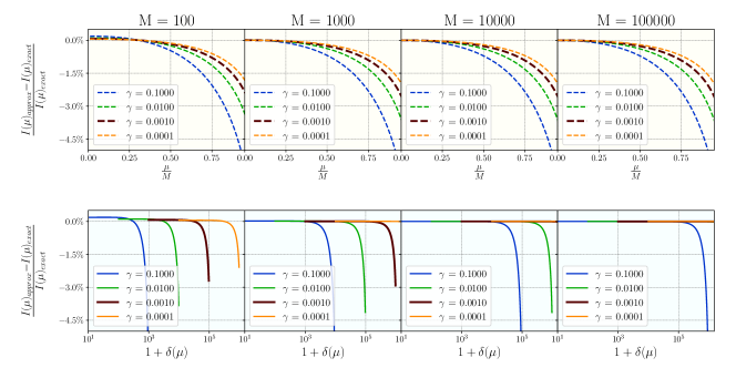
Figure 1: This figure shows the effect of the approximation proposed in Equation 5

This relation can be used to calculate the probabilities at each voxel in the mesh. However, with $\mathrm{m}$ as an integer, one can only deal with discrete distributions using Equation 4. To evaluate the expected probabilities for any fractional real values of $\mathrm{m}$, one requires an approximation

$$\prod_{i=0}^{\mu-1}{\left(\frac{M-i}{{\cal N}-i}\right)} = \left(\frac{M-\frac{\mu}{2}}{{\cal N}-\frac{\mu}{2}}\right)^{\mu};$$ (5)

where $\mathrm{m}$ is replaced by $\mu$, a continuous real-valued variable within $0\leq\mu<M$. The objective is to partition any continuous or discrete field into multiple virtual patches, referred to as ”chunks” hereafter, each possessing identical content but varying in morphology. Cumulatively, these chunks cover the entire volume in consideration. After employing the approximation, Equation 4 becomes

$$p\,(\,\mu\,) = \left(\frac{N_{v}-1}{{\cal N}-\mu}\right)\left(\frac{M-\frac{\mu}{2}}{{\cal N}-\frac{\mu}{2}}\right)^{\mu}.$$ (6)

Now, probability is closely related to information. Probability quantifies the likelihood of an event. On the other hand, information measures the reduction of uncertainty in a system or process through the outcomes. The information content corresponding to the probability of getting $\mu$ objects can be found as,

$$I\,(\,\mu\,) = -\log\,\left[\,p(\mu)\,\right]$$ (7)

$$= \log\left[\left(\frac{{\cal N}-\mu}{N_{v}-1}\right)\left(\frac{2{\cal N}-\mu}{2M-\mu}\right)^{\mu}\right].$$

Information is small for events with higher probabilities. On the contrary, unlikely events or configurations hold a large amount of information. The choice of the base of the logarithm here is arbitrary. In this work, we have used natural logarithms; so the information content has unit nats. However, later on the units are converted to terabytes using a conversion factor $u_{I}=\frac{2^{-43}}{\ln 2}$

Let us now introduce the parameter $\gamma$ to control the chunk-to-grid ratio. $\gamma=\frac{M}{N_{v}}$ is effectively the mean number density of chunks. The information content is now obtained as a function of $\mu$ and $\gamma$ by substituting $N_{v}$ with $\gamma$ in Equation 7, i.e.

$$I\,(\,\mu\,)=\ln\left[(1+\gamma)-\frac{\gamma(\mu-\gamma)}{M-\gamma}\right]+\mu\ln\left[1+\frac{2(M-\gamma)}{\gamma(2M-\mu)}\right].$$ (8)

We can also write $\mu$ in terms of the mean mass fraction $\bar{f}_{\cal M}$, where $\bar{f}_{\cal M}\,=\,\frac{\gamma}{M}$; i.e. the fraction of the total mass contributing to an individual voxel, on average. It also determines the grid resolution. After substituting $M$ with $\frac{\gamma}{\bar{f}_{\cal M}}$ we are left with

$$I\,(\,\mu\,)=\ln\left[(1+\gamma)-\frac{(\mu-\gamma)\,\bar{f}_{\cal M}}{(1-\bar{f}_{\cal M})}\right]+\mu\ln\left[1+\frac{1-\bar{f}_{\cal M}}{\left(\gamma-\frac{\mu\,\bar{f}_{\cal M}}{2}\right)}\right].$$ (9)

2.2 Information of large-scale Structures

So far in this section, we have not mentioned galaxies or Large-scale Structures. We started with $M$ discrete point objects having unique locations in terms of voxel indices. However, using further approximations, we now have $M$ extended chunks that span throughout the volume in consideration. Hence, they can partially contribute to more than one voxel. Now, let us consider $G$ galaxies distributed in the cubic volume, comprised of $N_{v}$ grids. We can virtually divide $G$ galaxies into $M$ chunks of equal weightage, each having $Q_{M}=\frac{G}{M}$ galaxies. If any given voxel contains $g$ galaxies, we will have $\mu=\frac{g}{Q_{M}}$.

Note that $(\frac{\mu}{\gamma}-1)$ is the fractional density contrast ($\delta$), at any given voxel, and equation Equation 9 can also be written in terms of $\delta$ as

$$I(\delta)=\ln\left[(1+\gamma)-\frac{\gamma\delta\bar{f}_{\cal M}}{1-\bar{f}_{\cal M}}\right]+\gamma(1+\delta)\ln\left[1+\frac{(1-\bar{f}_{\cal M})}{\gamma\left\{1-(1+\delta)\frac{\bar{f}_{\cal M}}{2}\right\}}\right].$$ (10)

$I(\delta)$ is the information associated with overdensity $\delta$ in the given matter distribution. Equation 10 displays a crucial relationship between the density perturbation and the Information associated with the large-scale structures. Hereafter any mention of information would mean this large-scale information. Equation 10 applies to both discrete and continuous fields since it no longer contains any explicit constraint of discreteness. When we started with $M$ and $N_{v}$ as integers, we could work only with discrete point data. However, one can now think of a continuous field that spans the entire volume but is virtually discretized into $M$ chunks of equal contribution. Equation 10 allows to work with extensive variables that contribute fractionally to the elementary volume. Nonetheless, one has to carefully choose ${\bar{f}_{\cal M}}$ and $\gamma$ depending on the clustering strength ($\delta$) of the distribution. The two terms in Equation 10 on which the logarithm is being operated must produce non-zero positive numbers. This can be easily taken care of by choosing sufficiently large $N_{s}$ or very small values of ${\bar{f}_{\cal M}}$. We also have to remember that the approximation presented in Equation 5 allows us to have the final form of Equation 10, and one has to be careful while using such an approximation. The limitation of this approximation is shown in Figure 1. For $\gamma<0.01$ and $M>100$ one can safely use the approximation with more than $99.9\%$ accuracy up to $\delta\leq 10^{4}$. However, for larger values of $\gamma$, it is necessary to have a large number of chunks in use.

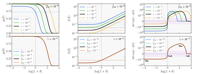
Figure 2: This figure shows probability [left], information [middle] and information gain [right] as a function of $\delta$ for different values of $\gamma$ and $\bar{f}_{\cal M}$. The two panels on the right show the identity inside the square brackets in Equation 15. Symmetric logarithmic scales are used along the vertical axis where the region with the purple shade has a linear scaling.

For a completely homogenous distribution, we would have $\delta=0$ at every grid. If $\bar{I}$ is the average information for a homogeneous distribution, then

$$\bar{I}=\ln\left(1+\gamma\right)+\gamma\ln\left[1+\frac{1-\bar{f}_{\cal M}}{\gamma\left(1-\frac{\bar{f}_{\cal M}}{2}\right)}\right]$$ (11)

is associated with the base probability of $\bar{p}=e^{-\bar{I}}$.

It is imperative to consider that the mass distribution of the universe has been discretely characterized based solely on the presence or absence of galaxies. Since galaxies occupy a minuscule portion of the total space, it is more probable to encounter empty regions than substantial overdensities. When comparing a galaxy cluster to an individual void, a unit volume extracted from a void contains less information than a unit volume from a cluster, owing to the vast size of voids. Nonetheless, the collective contribution from voids proves significant due to their higher likelihood of occurrence. Regardless of whether the unit volume is extracted from an under-dense or overdense region, uncertainty is always lost. Hence, departures from the mean background would lead to a change of information, which goes into shaping newly formed structures. However, the extent and direction of this information loss vary between overdense and under-dense structures.

At this point, we make another crucial assertion by imposing the holographic principle on the cube in consideration and define the total weighted   Information Gain   for any $i^{th}$ voxel as

$${\cal G}_{i}(\delta) = \frac{A_{c}}{4l_{P}^{2}}\left[\,\frac{p_{i}(\delta)\left\{\,I_{i}(\delta)-\bar{I}\,\right\}}{\bar{p}\bar{I}\,U_{0}}\,\right].$$ (12)

Here $A_{c}=6\left(\frac{L}{1+z}\right)^{2}$ is the surface area of the cube with its center at redshift $z$. The Planck length $l_{P}$ is derived from gravitational constant ($\,G\,$), Planck constant ($\,\hbar\,$) and speed of light ($\,c\,$) as $l_{P}=\sqrt{\frac{G\hbar}{c^{3}}}$. The total excess probabilities within the cube is denoted as $U_{0}=\sum_{i}\exp\{\bar{I}-I_{i}\}$. For a completely homogeneous distribution, the information gain for any voxel and the entire cube would be zero. We rewrite Equation 12 in terms of excess information $\Delta I_{i}=(I_{i}-\bar{I})$,

$${\cal G}_{i}(\delta) = \frac{K}{U_{0}\bar{I}}\left[\,\Delta I_{i}\,\exp\{\,-\Delta I_{i}\,\}\,\right].$$ (13)

$K=\frac{3u_{I}L^{2}}{2(1+z)^{2}l_{P}^{2}}$ is a constant for a specific cube, positioned at a given redshift. The factor $u_{I}=\frac{2^{-43}}{\ln 2}$ is used to convert the results from nats to terabytes. For overdense structures, we get +ve ${\cal G}$ and -ve ${\cal G}$ is obtained for under-dense spaces. As we have stated before, the growth of structures forces a system to lose information, which subsequently gets stored as the configuration of the emergent structure.

The right panels of Figure 2 shows ${\cal G}$ as a function of $\delta$ in symmetric log scale, for different choices of $\gamma$ and ${\bar{f}_{\cal M}}$. from the bottom right panel of this figure it is clear that ${\cal G}$ is not sensitive to ${\bar{f}_{\cal M}}$. For an infinitesimal ${\bar{f}_{\cal M}}$, Equation 10 and Equation 11 leads to

$$I(\,\delta\,)=\bar{I}+\frac{\delta}{\delta_{c}},$$ (14)

with $\,\delta_{c}=\left[\gamma\ln\left(1+\frac{1}{\gamma}\right)\right]^{-1}$ Equation 13 becomes

$${\cal G}(\delta)=\frac{K}{U_{0}\bar{I}}\left[\,\frac{\delta}{\delta_{c}}\exp\{-\frac{\delta}{\delta_{c}}\}\,\right],$$ (15)

The function ${\cal G}(\delta)$ has four characteristic points min, null, max and fall, at $\delta=-1$, $\delta=0$, $\delta=\delta_{c}$ and $\delta\sim 10\delta_{c}$ respectively. These critical points which define the curve are marked in the bottom right panel of Figure 2. Now, $\delta_{c}$ remains a free parameter unless we constrain it through observational evidence. In this work, we choose $\gamma={8}\times 10^{-4}$ to set $\delta_{c}\sim 175$ as this critical value represents the density threshold required for the virialization of a system. Past this threshold, the system configuration which has gradually developed over time through the externally acquired information, begins to be overridden by the internal stochasticity. Further increment in density contrast would cause the information gain to be suppressed and finally, it will diminish at the core ($\delta\to\infty$).

2.3 Information density and spectrum of information

We conduct a numerical analysis to search the scale of homogeneity in the SDSS galaxy distribution. After a cube of size $L$ is carved out from the SDSS survey volume ( as described in subsection 3.1 ), it is divided into $N_{s}^{3}$ voxels of size $\Delta x$. The density contrast for each voxel is then found from the effective galaxy count. We estimate information gain for each voxel using the relation in Equation 15. In this section, we do not impose $\bar{f}_{\cal M}\to 0$ and choose a finite value of $\bar{f}_{\cal M}$, as we are trying to validate the Cosmological principle itself. Figure 3 shows Information Gain at different locations within one of the cubes in Sample 1. It also presents how information gain correlates with galaxy clustering and respective probabilities. We use $N_{s}=50$ grids, setting $\bar{f}_{\cal M}={8}\times 10^{-6}$. So, there are $100$ virtual chunks in use.

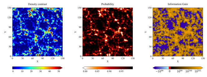
Figure 3: The density, probability and specific information gain is shown at different points of a $150{\,h^{-1}\,{\rm Mpc}}$ cube from SDSS ( Sample 1 ). A $30{\,h^{-1}\,{\rm Mpc}}$ slice in the $z$ direction is projected on the $X-Y$ plane.

After we have the Information gain calculated at each of the $N_{v}$ grids, we find the dimensionless 3D Information spectrum as the Fourier transform of information gain in the unitary form

$$\cal S(\mathbf{k}) = \int_{\mathbb{R}^{3}}{\Sigma(\mathbf{x})\,\exp\left\{-2\pi i\,\mathbf{k}\cdot\mathbf{x}\right\}}\,\,d^{3}x.$$ (16)

Here $\Sigma(\,\mathbf{x}_{i}\,)=\frac{{\cal G}_{SNC}(\,\mathbf{x}_{i}\,)}{\Delta x^{3}}$ is the information density with ${\cal G}_{SNC}$ as the shot noise corrected information gain ( see A ). $\cal S$ is a dimensionless complex quantity, computed using the Discrete Fourier Transform (DFT), i.e.

$${\cal S}_{[l,m,n]}=\frac{1}{\sqrt{N_{v}}}\sum_{l=0}^{N_{s}-1}\sum_{m=0}^{N_{s}-1}\sum_{n=0}^{N_{s}-1}\Sigma_{[a,b,c]}\;\exp\left\{\frac{-2\pi i}{N_{s}}(al+bm+cn)\right\}$$ (17)

Here $[a,b,c]$ are the indices for a specific voxel in the real-space; whereas, $[l,m,n]$ are indices for grids in Fourier space. The factor $\sqrt{N_{v}}$ ensures that Parseval’s identity is satisfied.

The available wave numbers in the Fourier space for a grid spacing $\Delta x$ and box size $L=N_{s}\,\Delta x$ are

$$k_{m} = k_{N}\left[\frac{2m}{N_{s}}-1\right];\quad\quad\text{for $\left\{m=0,1,2,\ldots,(N_{s}-1)\right\}$}$$ (18)

with $k_{N}=\frac{\pi}{\Delta x}$ as the Nyquist frequency.

Now, our goal is to find $\cal S$ as a function of $k$. We proceed by considering the entire available 3D $k$-space to be comprised of $N_{b}$ spherical shells centred at ($\frac{N_{s}}{2}$,$\frac{N_{s}}{2}$,$\frac{N_{s}}{2}$). Any $j^{th}$ shell is extended from $\frac{(j-1)\,\,k_{N}}{N_{b}}$ to $\frac{j\,\,k_{N}}{N_{b}}$, if $j$ takes values from $1$ to $N_{b}$. On the other hand, for any of the grid [$l$,$m$,$n$] in Fourier space, the magnitude of $k$ is found as $|\,k\,|=\sqrt{\,k_{l}^{2}+k_{m}^{2}+k_{n}^{2}\,}$. The spherical bin that the grid belongs to is then $b=\lfloor\frac{N_{b}\,|\,k\,|}{k_{N}}\rfloor$. For each bin, we calculate the 1D Information spectrum, $\bar{\cal S}(k)$ by taking a bin-wise average over $\cal S$, where each spherical bin has a specific value of $k$, associated with it. $\bar{\cal S}(k)$ now quantifies the average information gain across different frequencies.

2.4 Information sharing across different length scales

We perform an inverse-Fourier transform on $\bar{\cal S}$, normalizing it by the Nyquist frequency, to measure the Information gain shared by the space on different length scales,

$${{\cal G}^{M}}(\,r\,) = \frac{1}{k_{N}}\int_{-\infty}^{+\infty}{W(k)\cdot\bar{\cal S}(k)\,\exp\left\{2\pi ik\cdot r\right\}}\,\,dk.$$ (19)

${{\cal G}^{M}}(r)$ is called the Mutual gain, and it quantifies the average amount of uncertainty reduced by structure formation on length scale $r$. $W(k)$ is the window function that mitigates the effects from the finite volume and geometry of the region. Throughout this analysis, We have used a Kaiser window of the form

$$W(k)=\frac{i_{0}\left(\,\,\beta\sqrt{1-\left[\frac{k}{k_{N}}\right]^{2}}\,\,\right)}{i_{0}\left(\,\,\beta\,\,\right)}.$$ (20)

Here, $i_{0}$ is the modified Bessel function of the zeroth-order and $\beta=14$. The simplified form of Equation 19 in terms of DFT would be

$${{{\cal G}^{M}}}_{[a]} = \frac{1}{\sqrt{N_{b}}}\,\,\left[\sum_{m=0}^{N_{s}-1}W_{[m]}\,\,\bar{\cal S}_{[m]}\;\exp\left\{\frac{2\pi i\,a\,m}{N_{b}}\right\}\right]$$ (21)

Mutual gain essentially tells how much surplus information produced from the LSS formation is mutually shared by any two points in space, on average. The magnitude of ${{\cal G}^{M}}(r)$ signifies the extent of uncertainty reduction attributed to one point in space, due to the information stored at another point separated by a distance $r$. In the context of large-scale statistical homogeneity, by definition, the cause of information gain itself becomes redundant. Consequently, one would expect the mutual gain to exhibit a diminishing trend across the scale of homogeneity.

This section is concentrated on validating the existence of cosmic homogeneity and determining the length scale associated with it. So, the idea of a homogeneous universe has not been adopted thus far. To maintain causal consistency, our approach initially involved checking for the existence of cosmic homogeneity before its further application in the next part of the analysis.

2.5 Evolution of global information

In this section, we conduct an analytical exercise to study the evolution of global information content starting from $z=20$ up to $z=0$ in the $\Lambda CDM$ Universe. We consider the growth of the perturbations to follow the form $\delta(\mathbf{x},a)=D_{+}(a)\delta_{0}(\mathbf{x})$, as we focus on the linear perturbation regime by considering $\langle\delta^{2}_{0}(\mathbf{x})\rangle=\sigma_{8}^{2}$. Here $\delta_{0}(\mathbf{x})$ is the spatial profile of density contrast at present and $D_{+}(a)$ denotes the growing mode of matter density perturbations, which can be expressed as

$$D_{+}(\,a\,)=\frac{5\Omega_{m0}E(a)}{2}\int^{a}_{0}{\frac{da^{\prime}}{{a^{\prime}}^{3}E(a^{\prime})^{3}}},$$ (22)

with $E(a)=\frac{H(a)}{H_{0}}$ as the scaled Hubble parameter.

Let us now break down the assertion of $\bar{f}_{\cal M}\to 0$ which leads to Equation 15. Keeping $\gamma$ at a finite value, one has to keep adding voxels up to a point where all the virtual chunks that span the Universe are taken care of. This would require an enormously large number of voxels or an infinitesimal $\bar{f}_{\cal M}$. Hence, $\bar{f}_{\cal M}\to 0$ automatically imposes the assumption of cosmic homogeneity in this case.

At this point we introduce the global information entropy of the Universe as

$${\cal I}^{U}=\frac{K^{U}}{\bar{I}}\left[\frac{\int_{\mathbb{R}^{3}}\,p(\,\delta\,)\,I(\,\delta\,)\,d^{3}x}{\int_{\mathbb{R}^{3}}\,p(\,\delta\,)\,d^{3}x}\right],$$ (23)

with the redshift-dependent global maxima for information given as

$$K^{U}(z)=\frac{u_{I}c^{5}}{4G\hbar H_{0}^{2}}\left[\Omega_{m0}(1+z)^{3}+\Omega_{\Lambda}\right]^{-1}.$$ (24)

Now, $K^{U}(0)$ is the maximum amount of information that the present universe with a homogeneous matter distribution would contain, and this is $\sim 2.81\times 10^{147}\,\,terabytes$ of information. The global information entropy measures the effective information content in the Universe at a given time, considering the total information gain ( or loss ) caused by structure formation. Note that ${\cal G}^{U}$ being marginalized over space, is a function of the scalefactor (or redshift) only.

Before going forward, let us also introduce the functional exponentially weighted moment (EWM) at this point. The $k^{th}$ order EWM is defined as

$${\cal A}_{k}[\,\eta\,]=\frac{\int_{\mathbb{R}^{3}}\,\{\,\eta(\mathbf{x},a)\,\}^{k}\,\exp\{\,-\eta(\mathbf{x},a)\,\}d^{3}x}{\int_{\mathbb{R}^{3}}\,\exp\{\,-\eta(\mathbf{x},a)\,\}d^{3}x}.$$ (25)

With $a$ as the scalefactor and $\eta(\mathbf{x},a)=\frac{\delta(\mathbf{x},a)}{\delta_{c}}$ as the scaled contrast, we can now use Equation 14 and Equation 15 and rewrite Equation 23 as

$${\cal I}^{U} = K^{U}\left[\,1+\frac{{\cal A}_{1}}{\bar{I}}\,\right]$$ (26)

$$= K^{U}+{\cal G}^{U}\,\,,$$

where $K^{U}$ is the upper information bound and ${\cal G}^{U}(\,a\,)$ is the global information gain. We also term $(-\,{\cal G}^{U})$ as the global information loss hereafter. The rate of change of global information entropy with the scalefactor is

$$\frac{d{\cal I}^{U}}{da} = \frac{dK^{U}}{da}+\left(\frac{{\cal A}_{1}}{\bar{I}}\frac{dK^{U}}{da}+\frac{K^{U}}{\bar{I}}\frac{d{\cal A}_{1}}{da}\right).$$ (27)

The term inside the parenthesis on the right side of this equation gives the rate of change of information gain, i.e. $\frac{d{\cal G}^{U}}{da}$. Now, let us denote $\frac{d\ln K^{U}}{d\ln a}=\frac{3\Omega_{m}}{\Omega_{m}+\Omega_{\Lambda}}={\cal E}(\Omega_{m})$ with $\Omega_{m}=\Omega_{m0}a^{-3}$ and $\frac{1}{2}\left(\frac{5a}{3D_{+}}-1\right)=\Gamma(a)$. This allows the logarithmic growth rate ($\frac{d\ln D_{+}}{d\ln a}$) to be expressed as $\,\,f(\Omega_{m})=\Gamma(a)\,{\cal E}(\Omega_{m})\,\,$, and leads to

$$\frac{d{\cal G}^{U}}{da} = \frac{K^{U}\,{\cal A}_{1}\,{\cal E}}{a\,\bar{I}}\left[1+\Gamma\left\{1+{\cal A}_{1}-\frac{{\cal A}_{2}}{{\cal A}_{1}}\right\}\right],$$ (28)

through the $1^{st}$ derivative of the $1^{st}$ EWM ( see B ).

Equation 28 can be restructured in the following forms

$$\frac{d\ln{\cal G}^{U}}{d\ln a} = {\cal E}(\Omega_{m})\left[1+\Gamma\left\{1+{\cal A}_{1}-\frac{{\cal A}_{2}}{{\cal A}_{1}}\right\}\right],$$ (29)

$$\frac{d\ln{\cal G}^{U}}{d\ln H} = -2\left[1+\Gamma\left\{1+{\cal A}_{1}-\frac{{\cal A}_{2}}{{\cal A}_{1}}\right\}\right],$$ (30)

$$\frac{d\ln{\cal G}^{U}}{d\ln D_{+}} = \frac{1}{\Gamma}+\left\{1+{\cal A}_{1}-\frac{{\cal A}_{2}}{{\cal A}_{1}}\right\}$$ (31)

Note that Equation 30 presents the identity $-\frac{1}{(1+q)}\frac{d\ln{\cal G}^{U}}{d\ln a}$ with $q=-\frac{a\ddot{a}}{\dot{a}^{2}}$ being the deceleration parameter. The quantities listed above in combination are useful for validating the $\Lambda CDM$ model and cosmological parameter estimation since $A_{1}$ and $A_{2}$ can be readily determined from observations. However, this work only focuses on the overall evolution of information gain for a log-normal density distribution.

Let us now go back to Equation 25 and perform Taylor series expansion of the exponential terms, which gives the $k^{th}$ EWM in terms of the moments of $\eta(a)$; i.e.

$${\cal A}_{k}=\frac{\sum_{i=0}^{\infty}{\frac{(\,-1\,)^{i}}{i!}}\,\langle\,\eta(a)^{i+k}\,\rangle}{\sum_{i=0}^{\infty}{\frac{(\,-1\,)^{i}}{i!}}\,\langle\,\eta(a)^{i}\,\rangle},$$ (32)

where $\langle\eta(a)\rangle=0$, and $\langle\eta(a)^{2}\rangle=\frac{D_{+}^{2}(a)\sigma_{8}^{2}}{\delta_{c}^{2}}$.

Now, if we consider ($1+\delta$) to have a log-normal distribution with the skewness and kurtosis characterized by the $S_{p}$ parameters bernardeau95 (8), then the $3^{rd}$ and $4^{th}$ order moments of $\eta$ will be found as

$$\langle\eta(a)^{3}\rangle = \frac{S_{3}\sigma^{4}}{\delta_{c}^{3}},$$ (33)

$$\langle\eta(a)^{4}\rangle = \frac{S_{4}\sigma^{6}+3\sigma^{4}}{\delta_{c}^{4}},$$ (34)

where $\sigma\,=\,D_{+}\sigma_{8}$. The $S_{p}$ parameters at any given redshift $z$, are found as $S_{3}(z)=S_{3,0}(1+z)^{\alpha_{3}}$ and $S_{4}(z)=S_{4,0}(1+z)^{\alpha_{4}}$. The present values of $S_{3}$ and $S_{4}$ are $S_{3,0}=3+\sigma_{8}^{2}$ and $S_{4,0}=16+15\sigma_{8}^{2}+6\sigma_{8}^{4}+\sigma_{8}^{6}$ respectively. $\alpha_{3}$ and $\alpha_{4}$ control the rate of change of the skewness and kurtosis of the distribution at a given redshift. In this work, we have used $\alpha_{3}=-1.1$ and $\alpha_{4}=-2.3$ einasto21 (20) to study the evolution of global information entropy from $z=20$ to $z=0$.

3 Data

3.1 SDSS Data

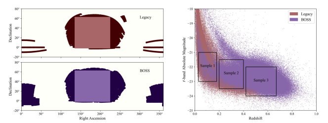
Figure 4: [Left]: $RA$-$DEC$ span in the SDSS sky that is chosen for sample preparation, using BOSS and Legacy data. [Right]: Definition of the quasi-magnitude-limited samples on the $redshift$-$mangitude$ plain.

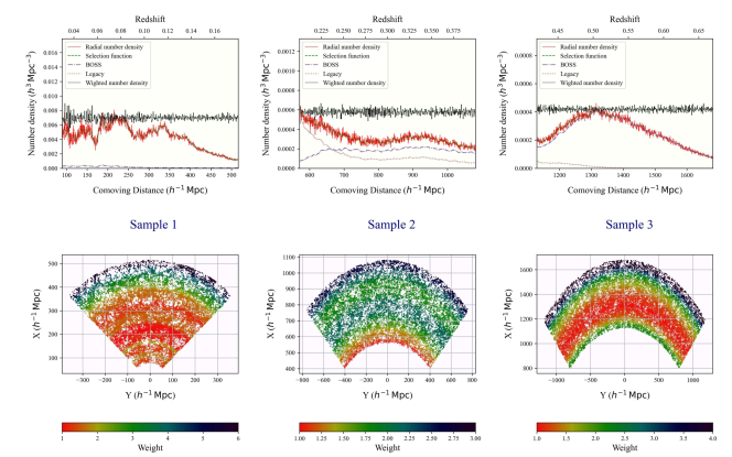
Figure 5: [Top]: The number-density variation of the three samples before and after applying the selection functions. [Bottom]: The distribution of the samples projected on the $X-Y$ plane for slices ( in $Z$ direction ) of width 10 times the mean-intergalactic-separation. Point sizes in the display are proportional to the respective weights.

Table 1: Description of the three samples prepared from SDSS data

	Sample 1	Sample 2	Sample 3
Absolute Magnitude	$-23\leq M_{r}\leq-21$	$-23.5\leq M_{r}\leq-21.5$	$-24\leq M_{r}\leq-22$
Redshift range	$0.03\leq z\leq 0.18$	$0.2\leq z\leq 0.4$	$0.42\leq z\leq 0.67$
Mean number density ($\bar{n}_{g}$)	${6.87}\times 10^{-3}{\,h^{3}\,{\rm Mpc^{-3}}}$	${5.70}\times 10^{-4}{\,h^{3}\,{\rm Mpc^{-3}}}$	${4.13}\times 10^{-4}{\,h^{3}\,{\rm Mpc^{-3}}}$
Size of cubes ($L$)	$150{\,h^{-1}\,{\rm Mpc}}$	$200{\,h^{-1}\,{\rm Mpc}}$	$250{\,h^{-1}\,{\rm Mpc}}$
Stride	$30{\,h^{-1}\,{\rm Mpc}}$	$40{\,h^{-1}\,{\rm Mpc}}$	$50{\,h^{-1}\,{\rm Mpc}}$
No. of available cubes	$201$	$1081$	$922$
Weighted count per cube	$23074\pm 2126$	$4643\pm 422$	$6584\pm 434$
Size of galaxy	$13.19\pm 4.66{\,{\rm kpc}}$	$23.95\pm 7.42{\,{\rm kpc}}$	$24.05\pm 10.45{\,{\rm kpc}}$
$u-r$ colour	$2.43\pm 0.72$	$3.78\pm 1.90$	$2.94\pm 2.03$
Redshift	$0.116\pm 0.021$	$0.306\pm 0.033$	$0.542\pm 0.039$
Distance from observer	$339.79\pm 46.42{\,h^{-1}\,{\rm Mpc}}$	$844.11\pm 61.72{\,h^{-1}\,{\rm Mpc}}$	$1416.89\pm 60.76{\,h^{-1}\,{\rm Mpc}}$

We use data from the Sloan Digital Sky Survey (SDSS) to find the information content associated with galaxy clustering in the observable Universe. Galaxy samples from three 3 different redshift zones are prepared using data from the $18^{th}$ data release almeida23 (3) of SDSS. DR18 incorporates refined data from all the prior programs of SDSS. However, we use data accumulated through the BOSS and the Legacy programs in this work. A Structured Query is used to retrieve the required data from SDSS Casjobs . To start with, conditions on the equatorial coordinates of the galaxies to choose galaxies within the angular span $135^{\circ}\leq RA\leq 225^{\circ}$ and $-2^{\circ}\leq Dec\leq 63^{\circ}$, as it provides a uniform sky coverage with high completeness. The left panel of Figure 4 shows the sky coverage of both BOSS and Legacy; the rectangular region shows the chosen span. In the first step, we prepare 3 quasi-magnitude-limited samples by applying constraints over the redshift range and the (K-corrected + extinction-corrected) $r$-band absolute magnitude ( right panel of Figure 4 ). The three conditions applied for the respective samples are tabulated in Table 1. This minimizes the variation in number density in the samples, reducing the Malmquist bias, due to which fainter galaxies are difficult to identify at higher redshifts. Note that the BOSS data we use here includes targets from both LOWZ ($0.15<z<0.43$) and CMASS ($0.43<z<0.70$). On the other end, we have Legacy data with higher incompleteness on small redshifts ($z<0.02$). Also, fibre collision will affect the selection of galaxies in close vicinity. Hence, choosing an appropriate magnitude and redshift range alone does not provide a completely uniform sample selection. The radial number density of the combined (BOSS+Legacy) distribution still exhibits background fluctuations in addition to the intrinsic variation in number density ( resulting solely from the growth of inhomogeneities in the matter density field ). To decouple the two effects we identify the radial selection function $n(r)$ by applying a Gaussian kernel ( $5\sigma$). The smoothed radial number density field now considered the selection function, represents the residual Malmquist bias that has to be filtered out. Using this selection function we assign a weight $w(r)$ to each galaxy lying in a given radial bin $r$ to $r+\delta r$. If $\bar{n}_{g}$ is the maximum value of the $n(r)$ within the entire range of radial comoving distance then $w(r)=\frac{\bar{n}_{g}}{n(r)}$. One must take the sum over the weights instead of adding a unit count for each galaxy. Put differently, for each galaxy found at the comoving radius $r$, we are also losing $w(r)-1$ neighbouring galaxies due to the limitations of the survey. The top panels of Figure 5 show the radial number density profile of the three samples, before and after applying the selection function. The bottom three panels show galaxy distributions in slices, from each of the three quasi-magnitude-limited samples, projected on the $X$-$Y$ plane; each point represents a galaxy and the point sizes are scaled proportionally with the respective weights. Note that the three samples have different values of $\bar{n}_{g}$; hence, the values of the weights are specific to the samples. The comoving Cartesian coordinates of each galaxy in the sample are found using the spectroscopic redshifts and equatorial coordinates. After we have the three samples, we carve out cubic regions of $150{\,h^{-1}\,{\rm Mpc}}$, $200{\,h^{-1}\,{\rm Mpc}}$ and $250{\,h^{-1}\,{\rm Mpc}}$ from Sample 1, Sample 2 and Sample 3, respectively. we curve out as many cubes as possible by taking successive strides in all three directions. Any two adjacent cubes share $80\%$ the side length or almost $50\%$ of their volume. Relevant information about three samples is tabulated in Table 1. For each sample, we have shown the (average) apparent size and $u-r$ colour of the constituent galaxies. The size is determined from the product of the angular diameter distance and the Petrosian radius ( in radians ) of the circle containing $90\%$ of its total light.

3.2 Nbody Data

We generate a number of dark matter distributions by running a cosmological N-body simulation with GADGET4 springel21 (54). The simulation is performed by populating $128^{3}$ dark-matter particles inside a $500{\,h^{-1}\,{\rm Mpc}}$ cube and tracking their evolution up to redshift zero. Ten realisations are generated and eight disjoint cubes are further extracted from each by dissecting them in each direction. We finally have $80$ cubes of size $250{\,h^{-1}\,{\rm Mpc}}$ for each of the redshifts that we have access to. To analyse the evolution of information content for $\Lambda CDM$ cosmology we analyse the distributions of dark-matter particles at redshifts $0$, $0.5$, $1$, and $2$. For each of the $80$ cubes, we randomly select $100000$ dark-matter particles to retain them in the final samples.

3.3 Biased distributions in redshift-space

3.3.1 redshift-space mapping

We take each of the $80$ N-body cubes for $z=0.5$ and introduce linear redshift-space distortions (RSD) by randomly placing the cubes within the accessible radial and angular span available for the SDSS data. The cubes are placed in such a way that the relative distance and orientation between the observer and the N-body cube centres mimic that of the SDSS (Sample 3) cubes. Using the velocities of each of the particles in the distribution we find their redshift-space coordinates as

$$\mathbf{s}=\mathbf{r}\,\left[1+\frac{\mathbf{v}\cdot\mathbf{r}}{a\,H(a)\,\,||\mathbf{r}||^{2}}\right],$$ (35)

where $\mathbf{v}$ and $\mathbf{r}$ are the actual velocity and position vectors in real-space. $z=0.542$ is used for finding the scalefactor ($a$) and Hubble parameter, $H(a)$ to plug into the above equation.

3.3.2 Biased distribution

Galaxies are formed after baryonic matter follows the pre-existing DM halos to select the density peaks for consolidation preferentially. So they are considered to be positively biased by and large. We use the N-body data to mimic a couple of biased galaxy distributions along with unbiased and negatively biased ones as well. To apply the bias on the redshift-space distribution of DM particles, we use the selection function (model 1) proposed by cole98 (13). For a given cube of dark-matter particles mapped in redshift-space, We apply a Cloud-In-Cell (CIC) technique with a mesh of $N_{c}^{3}$ grids to measure the density contrast ($\delta$) on the grids. Thereafter, the z-score of density contrast, $\nu(x)=\frac{\delta(x)-\mu}{\sigma}$ is found for each of the particles, where $\sigma=\sqrt{<\delta^{2}>}$ and $\mu=\langle\delta\rangle=0$. We then apply trilinear interpolation to determine $\nu$ at the particle positions from the $8$ adjacent grids. Next, the selection probability

$$p_{s}(\nu)\,=\,\begin{cases}\exp\,(\,A\nu+B\nu^{\frac{3}{2}}\,),&\text{if }\nu\geq 0\\ \exp\,(\,A\nu\,),&\text{if }\nu\leq 0\end{cases}$$

is applied to have a density-wise biased selection of the particles from the entire cube. We also find the base probability of the particles $p_{0}(\nu)=\frac{(1+\nu\sigma)}{N_{c}^{3}}$; i.e. the probability of finding a randomly selected particle to have contrast $\nu$. After applying the selection function, the selection probability of a particle with scaled contrasts $\nu$ into the final set is $p_{f}(\nu)=p_{0}(\nu)\,p_{s}(\nu)$. Next, a random probability $p_{r}$ between 0 and $max\{p_{f}(\nu)\}$ is generated for each particle in the distribution. The particles which satisfy the criteria $p_{r}<p_{f}$ are selected to represent the galactic mass. We randomly select $100000$ particles, to get the final samples from each biased and unbiased distribution for further testing effects of linear RSD and biasing. The density contrast ($\delta$) is calculated ( by using CIC ), for each particle in the newly formed biased samples. Finally, linear bias is estimated by comparing their $\delta$ profile with the unbiased sample. We use different combinations of $A$ and $B$ and then check the linear bias for the distribution using the technique described in C. The parameters are tweaked to achieve the desired values of $b_{1}$ through trial and error.

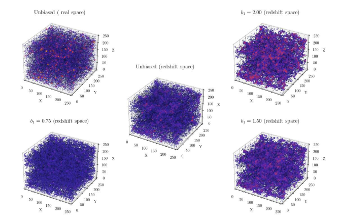
Figure 6: The distribution of the different mock samples ($z=0.5$) described in subsection 3.3, before and after applying RSD and bias. Distribution for three different bias values is shown along with the original distribution and its counterpart in redshifted space. The variation in density contrast is represented using the variable colour palette.

The suitable values of the parameters $A$ and $B$ which provide the desired values of linear bias $b_{1}$ are enlisted in Table 2. Figure 6 helps compare the redshift-space biased and unbiased distributions with the original real-space N-body data. All distributions have the same number of particles.

Table 2: Specifications for the mock biased distributions from redshifted N-body cubes.

$A$	$B$	Linear bias ($b_{1}$)
		Target	Model
$1.0$	$-2.51$	$0.75$	$0.755\pm 0.008$
$1.5$	$-1.11$	$1.50$	$1.505\pm 0.014$
$2.0$	$-1.20$	$2.00$	$1.990\pm 0.019$

4 Results

4.1 Information Spectrum and Information Sharing

In subsection 2.3, we discuss how to track the distribution of information gain in different frequencies through the information spectrum. On the other hand, the average information gain shared between two points separated by a certain distance in space is measured through the mutual gain, which is presented in subsection 2.4. At first, we take the 3 samples from SDSS and analyze the distribution of information in the observable Universe. We carry out the same analysis for simulated N-body data at different redshifts and further check the effect of linear RSD and bias by comparing SDSS results with redshift-space biased N-body mock distributions. For each case, we search for the scale of homogeneity where the mutual gain goes to zero.

4.1.1 Large-scale information sharing and scale of homogeneity

In the top-left panel of Figure 7, the information spectrum is presented for three samples representative of three redshift zones. We notice a higher degree of information gain is associated with the larger wavelengths (small $k$) for all three samples. The amplitude gradually falls with increasing $k$ and finally reaches a plateau at the high-frequency end. We notice an abrupt change in the slope of the information spectrum near $0.06{\,h\,{\rm Mpc^{-1}}}$ for all three samples. This fall in spectral amplitude persists up to the nonlinear regime ($>0.78{\,h\,{\rm Mpc^{-1}}}$); after which, the consistent drop in information slows down and remains steady up to the smallest scales probed. This non-diminishing tail is the characteristic signature of information gain. Due to the presence of the exponential term, it contains all higher-order moments of density perturbations. Hence, it is capable of tracing the collective information offsets caused by all the multi-point correlations existing in that space of relevance. We find that Sample 2 has a nearly identical profile as Sample 3, but $\sim 7\%$ more information on higher frequencies. Sample 1 has a relatively lower information gain than Sample 2 and Sample 3 on all wavelengths. This is non-intuitive at first sight. On lower redshifts, the amplitude of information gain is expected to get higher with the enhancement in the definition of the structures. However, for Sample 1, we observe the information gain to be falling more rapidly in the large $k$ range. The presence of redshift-space distortions partly explains this fall. which is explained later in detail. However, the primary reason for this decline is that Sample 1 is a collection of a different class of galaxy than the other two samples. From Table 1, we find that galaxies in Sample 1 are much smaller in size compared to the galaxies in the other two samples. A relatively higher absolute magnitude and bluer $u-r$ color also indicate the presence of a younger population in the galaxy sample. This means that, unlike the other two samples, Sample 1 consists of a fair number of field and satellite galaxies that are not representative of a higher degree of clustering and hence cause less information gain.

The bottom-left panel of Figure 7 shows the spectral index of information gain. If the information spectrum follows the relation $\bar{\cal S}\propto k^{n_{s}-1}$, then the spectral index of information gain is given as $n_{s}(k)=\frac{\Delta\ln{\bar{\cal S}}}{\Delta\ln k}+1$. For all the samples, we find $n_{s}$ lying between $0$ and $1$, with a red-tilt that points toward an inside-out picture of information sharing. The spectral index starts with $n_{s}=1$ at the smallest $k$ we probe. This shows a scale-independent nature of the information spectrum on the largest scales or earliest epochs. It then gradually starts reducing, eventually reaching a turnaround point where $n_{s}$ finds its minimum value. This is where information gain has the maximum scale dependence. For Sample 2 and Sample 3, we can find this turnaround near $0.2{\,h\,{\rm Mpc^{-1}}}$. For Sample 1 however, we see this drop with a much lower value of the spectral index ($n_{s}\sim 0.1$) and in a relatively higher frequency range ($0.3-0.5{\,h\,{\rm Mpc^{-1}}}$) where $\bar{\cal S}$ becomes almost inversely proportional to $k$. In other words, bigger the structure, greater the information it contains.

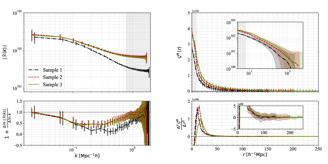
Figure 7: [Top-left]: Information spectrum as a function of wave numbers. [Bottom-left]: This Figure shows the spectral index $n_{s}$, at different values of $k$. [Top-right]: Information sharing as a function of length scales. The same thing is shown in the inset but in the log-scale. [Bottom-right]: Slope of information sharing. A zoomed-in view is presented in the inset.

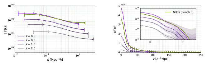
Figure 8: [Left]: Information spectrum as a function of wave numbers for the N-body dark-matter distributions simulated at different redshifts. The SDSS data (Sample 3) is shown alongside. [Right]: Information sharing as a function of length scales, for the same distributions.

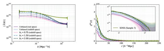
Figure 9: Same as Figure 8 but for redshift-space biased distributions. The original real-space distribution, the redshift-space unbiased distribution and the SDSS Sample 3 are also shown for comparison.

The top-right panel of Figure 7 shows the mutual gain as a function of length scale. The large information sharing found on small scales ($<10{\,h^{-1}\,{\rm Mpc}}$) advocates the coherence of the local structures. Two points in close vicinity share a similar fate regarding the evolution of their neighbourhood; hence, there is a maximum reduction in uncertainty on smaller scales, resulting in high information gain. As we go towards higher length scales information sharing falls $60-70\%$ up to $20{\,h^{-1}\,{\rm Mpc}}$. The sharp peaks that feature in the $\frac{\Delta^{2}{\cal G}^{M}}{\Delta r^{2}}$ vs $r$ plot (bottom right panel of Figure 7), correspond to the length-scale for the sharpest fall. As we can notice, this characteristic scale is slightly different for each sample and is connected to their mean intergalactic separation. Beyond this scale, the existing coherence gets rapidly weakened. In Sample 1, the average information sharing approaches zero at about $\sim 140{\,h^{-1}\,{\rm Mpc}}$. However, the mean ${\cal G}^{M}$ does not completely diminish for Samples 2 and 3 anywhere within the scope. Nevertheless, while examining the second derivatives, we observe that $\frac{\Delta^{2}{\cal G}^{M}}{\Delta r^{2}}$ for Sample 2 and 3 gradually approaches zero, exhibiting a steadily reducing amplitude. This implies that $\frac{\Delta{\cal G}^{M}}{\Delta r}$ is getting closer to a constant value. Now, from the ever-reducing trend for the ${\cal G}^{M}(r)$, at the largest available length scales, with a constant slope, will force the mutual gain eventually diminish at a certain length scale. This scale however is beyond the explored extent for these two samples. Note that galaxies separated by a distance beyond the scale of homogeneity cannot affect the reduction in uncertainty about their prospective evolutionary trajectories.

4.1.2 Information Sharing at different redshifts

We use N-body simulations to study the information distribution at different redshifts in a $\Lambda CDM$ Universe. We went over $80$ N-body realisations of the distribution of DM particles at redshifts of $0$, $0.5$, $1$, and $2$ ( see subsection 3.2 ). For a fair comparison, we compare the results with sample 3 (SDSS), since each cube has the same size of $250{\,h^{-1}\,{\rm Mpc}}$. Figure 8 shows that the overall amplitude of both information spectrum and mutual gain is much higher in sample 3 compared to the N-body cubes. One might expect the Sample 3 results to be substantially closer to $z=0.5$, but the mutual gain for Sample 3 is almost twice the $z=0.5$ distributions. The unfair comparison we are making between the information content of galaxy and DM distributions here is the cause of this difference. This is addressed in the next section. The characteristic that stands out in this case is the information content gradually increasing across all length scales with decreasing redshifts. Additionally, the homogeneity scale for the N-body cubes drops as we go towards higher redshifts. These findings are rather typical. The offset from a homogenous random background would increase with decreasing redshift, as the structures are better defined and less arbitrary on lower redshifts. Incoherent structures with greater uncertainty are less likely to contribute to the reduction of uncertainty at other distant points in the space. Hence, the scale of homogeneity is naturally expected to drop for distributions at higher redshifts. The results in Figure 8 are consistent with this expectation. For all the N-body cubes homogeneity is achieved within $130{\,h^{-1}\,{\rm Mpc}}$; whereas, the SDSS Sample 3 distribution tends towards homogeneity beyond $160{\,h^{-1}\,{\rm Mpc}}$.

4.1.3 Effect of linear bias and redshift-space distortions

Figure 9 presents the en bloc effect of RSD and bias on the information distribution. In the left panel of the figure, we show the information spectra of the distributions with and without RSD and biasing. Let us first compare the real-space and redshift-space unbiased distributions. We observe that the redshift-space distribution exhibits suppression of information on higher frequencies, whereas enhancement in the information spectrum can be noticed for larger wavelengths. The first effect is the manifestation of the Finger-of-God (FOG) effect, and the second one is caused by the Kaiser effect; both of these are effects of RSD. The random peculiar motion of galaxies in dense environments such as galaxy clusters causes the elongation of the apparent shape of structures along the line of sight. This FOG effect reduces the coherence of the particles in close vicinity, that exist in the real-space distribution, causing the signal to drop on higher frequencies. On the contrary, on large scales, galaxies experience bulk infall towards large overdensities, causing galaxies to appear closer to each other than they are. Hence artificial spatial coherence is introduced in the signal on large scales. This also explains the observed fall of information for Sample 1 in the top-left panel of Figure 7. Both the distance of the observer and the clustering of particles affect the degree of information suppression on large $k$. The suppression would increase with increasing density contrast and proximity of the observer relative to the cube. Unlike RSD, the effect of biasing does not affect the information in a high $k$ regime. Only the large-scale information gain is affected due to biasing. Information is found to be enhanced with biasing strength and this effect becomes more prominent as we move towards smaller $k$ values. However, the difference between the information spectrum of Sample 3 and the biased distribution for $k>0.1{\,h\,{\rm Mpc^{-1}}}$ is prominent and the difference increases with $k$. This tells us that a non-linear and scale-dependent biasing is required to model the information spectrum of the observed galaxy distributions, especially for a non-linear perturbation regime.

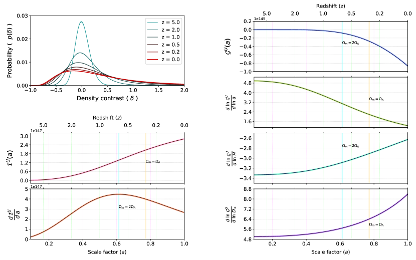
Figure 10: This figure shows the evolution of effective information entropy for a lognormal density distribution, from redshifts $20$ to the present day.

On the right panel of this figure, we show the information sharing for the different distributions. We also notice the enhancement in uncertainty when anti-biasing is applied, this reduces the information gain for the distribution with $b_{1}=0.75$, in all wavelengths. As we keep the bias increasing, the dark-matter particles are stripped away from the existing uncertainty, and a significant information gain is observed. For $b_{1}=2$, we find the redshifted distribution to come within 1-$\sigma$ of the SDSS Sample3 distribution. A reduced-$\Chi^{2}$ of $0.41$ suggests with a $99.99\%$ confidence level that the two distributions represent the same population. Both the real-space unbiased and redshift-space anti-biased distributions reach homogeneity within $120{\,h^{-1}\,{\rm Mpc}}$ whereas the distributions with $b_{1}=1$, $b_{1}=1.5$ and $b_{1}=2$ in redshift space achieve homogeneity around $150-160{\,h^{-1}\,{\rm Mpc}}$. Compared with the $b_{1}=2$ distribution one can expect the SDSS sample 3 distribution to reach homogeneity around $160{\,h^{-1}\,{\rm Mpc}}$. Although large standard deviations beyond $100{\,h^{-1}\,{\rm Mpc}}$ do not allow us to have a unanimous confirmation on a global homogeneity scale within this scope, we can at least rule out its presence in the observable Universe up to $130{\,h^{-1}\,{\rm Mpc}}$. It is also noteworthy that a characteristic scale where mutual gain is nullified does not imply causal disassociation.

4.2 Evolution of Global Information entropy

In subsection 2.5 we discuss the method to measure the global information entropy at a given epoch for a log-normal density distribution and introduce three dimensionless quantities $\frac{d\ln{\cal G}^{U}}{d\ln a}$, $\frac{d\ln{\cal G}^{\prime}}{d\ln H}$ and $\frac{d\ln{\cal G}^{U}}{d\ln D_{+}}$ to analyse the evolution of effective information gain of the universe. These logarithmic derivatives measure how fast or slow the Information gain changes relative to the growth rate of matter density perturbation or expansion rate of the space. In Figure 10 we show these quantities as a function of redshift or scalefactor.

The top left panel of Figure 10 shows the evolution of the density distribution that causes the change in the global information gain. The middle-left panel shows the overall information entropy of the Universe at different epochs. The present Universe holds $\sim 2.8\times 10^{147}TB$, including the observed -ve information gain ( or information loss) due to structures formed at $z=0$. In the bottom-left panel, we show the rate of change of ${\cal I}$ as a function of the scalefactor. We notice that $\frac{{d\cal I}^{U}}{da}$ rapidly increases during the cosmic noon ($1.5\lesssim z\lesssim 3$) and then slows down to reach the maximum at $z=0.63$; This is the point at which the expansion of the universe switches from a decelerated to an accelerated phase. Between $z=2$ to $z=0.5$ information entropy undergoes a huge $\sim 300\%$ increment; whereas, it grows only $\sim 75\%$ from $z=0.5$ to $z=0$, as the matter domination gets over. At the current epoch, ${\cal I}^{U}$ is found to be increasing in a decelerated way. This is the opposite of what information gain is undergoing at present. The information loss appears to be accelerating as seen by the top-left panel. Although the information loss is significantly smaller than the effective information entropy till now, we find that $\sim 8\times 10^{144}TB$ information has already been used in large-scale structure formation. Note that this accounts only for the linear perturbations of the matter density field and the expenditure could be greater when one incorporates structures on smaller length scales ($<8{\,h^{-1}\,{\rm Mpc}}$). However, information gain is insensitive to perturbations beyond $\delta\sim 200$, so we expect the actual loss to be close to the measured value.

The second panel from the top shows the logarithmic derivative of information gain w.r.t the scale factor. The information gain increases $5$ times as fast as the scale factor in the early Universe but slows down with the end of matter domination. The Information gain is growing by $1.5$ times as fast as the expansion rate in present times. The second panel from the top shows how sensitive the relative change in information gain is w.r.t the acceleration of the Universe. Now $(-\,{\cal G}^{U})\leq 0$ and $H(a)\geq 0$ throughout, which leave us with $\frac{d(-{\cal G}^{U})}{dH}<0$. Hence, the information loss is overall decreasing with the growth in expansion rate and the relative change in the information loss is $2.5$ times faster than the relative change in the Hubble parameter. Moving to the bottom-right panel, we notice the relative growth of ${\cal G}^{U}$ to be $5$ times higher in comparison with the change in growing mode, at $z\geq 4$; it then gradually increased and becomes almost $9$ times of the relative change in the growing mode. The crucial thing to note here is $\frac{d(-{\cal G}^{U})}{dD_{+}}>0$. This suggests that despite the expansion of the Universe the growth of structures will always cause a loss in information unless $f(\Omega_{m})\leq 0$. Note that both information gain and information loss are associated with reduction of uncertainty. The -ve sign of information gain associates the effective entropic change with a higher degree of information reduction in underdense regions.

5 Conclusion

The two-point correlation function and its Fourier counterpart the power spectrum are the widely used statistics for studying galaxy clustering. However, these two estimators and their multiple variants that rely upon a finite number of moments of density perturbation, may not be sufficient in analysing the galaxy and dark-matter clustering in the non-linear regime. We introduce the information gain, an information-theoretic identity that uses all the higher-order moments of perturbation in analysing the nature of clustering in the observable galaxy distribution. We employ this tool to analyse the real and Fourier space distribution of information in 3 different galaxy samples prepared using data from SDSS, each representing a specific redshift zone and a particular class of galaxy. This provides an idea of the information flowing through different parts of the cosmic web. We also quantify the information reduction mutually caused by structures at any two points in space, in the accessible volume. We search for a universal scale of homogeneity, where ( by definition ) the mutual gain in information diminishes irrespective of the local clustering strength. The presence of such a characteristic scale is not found at least up to $130{\,h^{-1}\,{\rm Mpc}}$. Furthermore, to study the evolution of the Universe’s information content, we study a log-normal density distribution that evolves with time. With redshift-dependent variance, skewness and kurtosis, it mimics the probability distribution of the actual density contrast in the matter density field. It is found that the growth of structures inevitably causes a reduction in information, irrespective of the expansion rate of the Universe. Although we have limited our discussion to the $\Lambda CDM$ cosmology, it is possible to examine the global information content of different cosmological models and constrain the cosmological parameters with the aid of appropriate observables. In this work, we have assumed that the characteristic change in total information entropy after $z=0.6$ is due to the matter component being dominated by dark energy. However, a converse scenario might also be true. Entropy being one of the fundamental physical entities in the Universe could cause the observed accelerated expansion itself. Detailed studies are required to comprehend the actual reason. This paper is meant to be the initial step, laying the foundation for future research that will build on it and will be better equipped to address these issues.

6 Data-availability

The data utilized in this study can be found in the SDSS database, which is open for public access. Data generated in this work can be shared on request to the author.

7 Acknowledgement

I thank Prof. Somnath Bharadwaj, Prof. Sayan Kar, Dr. Biswajit Pandey and fellow researchers at IIT-Kharagpur, for their suggestions and useful discussions. Special thanks to DST-SERB for support through the National Post-Doctoral Fellowship (PDF/2022/000149). Funding for the Sloan Digital Sky Survey IV has been provided by the Alfred P. Sloan Foundation, the U.S. Department of Energy Office of Science, and the Participating Institutions. SDSS-IV acknowledges support and resources from the Center for High Performance Computing at the University of Utah. The SDSS website is www.sdss.org. SDSS-IV is managed by the Astrophysical Research Consortium for the Participating Institutions of the SDSS Collaboration including the Brazilian Participation Group, the Carnegie Institution for Science, Carnegie Mellon University, Center for Astrophysics — Harvard & Smithsonian, the Chilean Participation Group, the French Participation Group, Instituto de Astrofísica de Canarias, The Johns Hopkins University, Kavli Institute for the Physics and Mathematics of the Universe (IPMU) / University of Tokyo, the Korean Participation Group, Lawrence Berkeley National Laboratory, Leibniz Institut für Astrophysik Potsdam (AIP), Max-Planck-Institut für Astronomie (MPIA Heidelberg), Max-Planck-Institut für Astrophysik (MPA Garching), Max-Planck-Institut für Extraterrestrische Physik (MPE), National Astronomical Observatories of China, New Mexico State University, New York University, University of Notre Dame, Observatário Nacional / MCTI, The Ohio State University, Pennsylvania State University, Shanghai Astronomical Observatory, United Kingrand-designom Participation Group, Universidad Nacional Autónoma de México, University of Arizona, University of Colorado Boulder, University of Oxford, University of Portsmouth, University of Utah, University of Virginia, University of Washington, University of Wisconsin, Vanderbilt University, and Yale University.

Appendix A Shot noise correction for Information gain

Consider a discrete distribution of ${\cal N}$ galaxies confined in a finite cubic volume, where each of the voxels accommodates $\bar{f}_{\cal M}\,\cal{N}$ galaxies on average. From Equation 15 for any $i^{th}$ voxel we get the information gain as

$${\cal G}^{(i)}=\frac{K}{U_{0}\bar{I}}\left[\Delta I^{(i)}\,\exp\{\,-\Delta I^{(i)}\,\}\right]$$ (36)

where $\Delta I^{(i)}=\frac{\delta(\mathbf{x}_{i})}{\delta_{c}}$.

With $n=(1+\delta)\,\bar{f}_{\cal M}\,\cal{N}$ as the count in a given voxel and $\sigma^{2}_{n}$ as the variance of the galaxy count, we estimate the shot-noise corrected $\Delta I$, i.e.

$$\Delta I_{SNC}(\delta)=\Delta I(\delta)-\left|\frac{\partial\,\Delta I}{\partial n}\right|\sigma_{n}$$ (37)

Now, $\frac{\partial\,\Delta I}{\partial n}=\frac{1}{\delta_{c}\,\bar{f}_{\cal M}\,\cal{N}}$, and if we assume the particle count to follow a Poisson distribution, then $\sigma_{n}=\sqrt{\bar{f}_{\cal M}\,\cal{N}}$. Hence, the shot noise correction would lead us to

$${\cal G}^{(i)}_{SNC}(\eta) = \frac{K}{\bar{I}\,U_{0}^{SNC}}\left[\Delta I^{(i)}_{SNC}\,\exp\{\,-\Delta I^{(i)}_{SNC}\,\}\right]$$ (38)

with $U_{0}^{SNC}=\sum_{i}\exp\{-\Delta I_{SNC}^{(i)}\}$ and

$$\Delta I^{(i)}_{SNC}=\Delta I^{(i)}-\frac{1}{\delta_{c}\sqrt{\bar{f}_{\cal M}\,\cal{N}}}$$ (39)

Appendix B Finding $n^{th}$ order derivative of $k^{th}$ EWM

Let us start by writing the $k^{th}$ EWM as

$${\cal A}_{k}=\frac{U_{k}}{U_{0}}$$ (40)

Where

$$U_{k}=\int_{\mathbb{R}^{3}}\eta^{k}e^{-\eta}d^{3}x$$ (41)

By definition $\eta(\mathbf{x},a)=D_{+}(a)\frac{\delta(\mathbf{x})}{\delta_{c}}$; hence we can deduce

$$\mathbb{D}^{q}\eta=\eta Q_{q}.$$ (42)

by denoting $\,\,\frac{d^{q}}{da^{q}}$ as $\mathbb{D}^{q}\,\,$ and $\,\,\frac{1}{D_{+}}\frac{\partial^{q}D_{+}}{\partial a^{q}}$ as $Q_{q}\,\,$. Note that $D_{+}$ being a function of $a$ alone allows the partial and total derivatives to have interchangeable connotations. Equation 42 also leads to the identities

$$Q_{0} = 1,$$

$$Q_{1} = \frac{f(\Omega_{m})}{a},$$

$$\mathbb{D}^{1}Q_{n} = Q_{n+1}-Q_{n}Q_{1},$$

$$\mathbb{\mathbb{missing}}{D}^{q}Q_{n} = {D}^{q-1}Q_{n+1}-\sum_{j=0}^{q-1}{}^{q-1}C_{j}\,\,\,\mathbb{D}^{q-j-1}Q_{n}\,\,\,\mathbb{D}^{j-1}Q_{1}.$$

We use Leibniz’s general product rule of differentiation to get the last equation.

Using Equation 43 the first derivative of $U_{k}$ is found as

$$\mathbb{D}^{1}U_{k}=Q_{1}\,[\,kU_{k}-U_{k+1}\,],$$ (43)

and the $1^{st}$ derivative of ${\cal A}_{k}$ would be

$$\mathbb{D}^{1}{\cal A}_{k} = \left[\,\frac{\mathbb{D}^{1}U_{k}}{U_{0}}-\frac{U_{k}\,\mathbb{D}^{1}U_{0}}{U^{2}_{0}}\,\right]$$ (44)

$$= Q_{1}\,[\,k{\cal A}_{k}-{\cal A}_{k+1}+{\cal A}_{1}{\cal A}_{k}\,]$$ (45)

Any $n^{th}$ order derivative of ${\cal A}_{k}$ can now be written as

$$\mathbb{D}^{n}{\cal A}_{k}=\mathbb{D}^{n-1}\left\{Q_{1}\,[\,k{\cal A}_{k}-{\cal A}_{k+1}+{\cal A}_{1}{\cal A}_{k}\,]\right\}$$ (46)

Finally, the $n^{th}$ derivative ( w.r.t $a$) of the $k^{th}$ EWM is found in form of the general recurrence relation

$$\mathbb{D}^{n}{\cal A}_{k} = \sum_{q=0}^{n-1}\,\,{}^{n-1}C_{q}\,\,\,\mathbb{F}^{n-q-1}_{1}\cdot\mathbb{T}^{q}_{k}.$$ (47)

$$\text{where}\,\,\,\mathbb{F}^{n-q-1}_{s} = \mathbb{D}^{n-q-1}Q_{s}\,\,$$

$$\text{and}\,\,\,\mathbb{T}^{q}_{k} = k\,\mathbb{D}^{q}{\cal A}_{k}\,-\,\mathbb{D}^{q}{\cal A}_{k+1}\,+\,\sum_{j=0}^{q}{}^{q}C_{j}\,\,\mathbb{D}^{q-j}{\cal A}_{k}\,\,\mathbb{D}^{j}{\cal A}_{1}$$

One can find the following identities using Equation 47.

$$\mathbb{D}^{1}{\cal A}_{1} = Q_{1}\left\{{\cal A}_{1}-{\cal A}_{2}+{\cal A}^{2}_{1}\right\}$$

$$\mathbb{D}^{1}{\cal A}_{2} = Q_{1}\left\{2{\cal A}_{2}-{\cal A}_{3}+{\cal A}_{2}{\cal A}_{1}\right\}$$

$$\mathbb{D}^{2}{\cal A}_{1} = Q_{1}^{2}\left\{2{\cal A}_{1}^{3}+{\cal A}_{1}^{2}-3{\cal A}_{1}{\cal A}_{2}-2{\cal A}_{2}+{\cal A}_{3}\right\}$$

$$+Q_{2}\left\{{\cal A}_{1}-{\cal A}_{2}+{\cal A}^{2}_{1}\right\}$$

Appendix C Scale independent estimation of linear bias

Let us consider the normalised probability distributions of $\delta$ for the unbiased and biased distributions to be $p^{u}(\delta)$ and $p^{b}(\delta)$ respectively. We divide the entire range of $\delta$ into $N_{\delta}$ bins. If the probabilities for the unbiased distribution in the $i^{th}$ and $j^{th}$ bins of $\delta$ are $p_{i}^{u}$ and $p_{j}^{u}$ respectively, then the joint probability of $(\delta_{i},\delta_{j})$ pairs to be found in the distribution would be proportional to $p^{u}_{i}\delta^{i}\cdot p^{u}_{j}\delta^{j}$. Using these joint probabilities, we propose a scale-independent linear bias estimator

$$b_{1}=\sqrt{\frac{\sum_{i}\sum_{j}p^{u}_{i}\delta_{i}\cdot p^{u}_{j}\delta_{j}}{\sum_{i}\sum_{j}p^{b}_{i}\delta_{i}\cdot p^{b}_{j}\delta_{j}}}$$ (48)

to measure the average linear bias of the newly formed distribution obtained after applying the selection function. Note that, $p^{u}$ and $p^{b}$ both are normalized so $\sum_{i}\sum_{j}p^{u}_{i}p^{u}_{j}=\sum_{i}\sum_{j}p^{b}_{i}p^{b}_{j}=1$. We choose $N_{\delta}=1000$ for this work.

Appendix D Information at a particular point in space with specific density contrast

The information required for finding an overdensity $\delta$ inside a cube with a known configuration is given in Equation 10 where the corresponding probability is $p(\delta)$. However, the joint probability of finding an object at a location $\mathbf{x}$ with density contrast $\delta$ would be $p(\,\mathbf{x},\delta\,)$. Given there are ${\bar{f}}_{\cal M}^{-1}$ voxels in the cube, the conditional probability of finding an object at $\mathbf{x}$ with the prior confirmation on the density contrast being $\delta$ would be $p(\,\mathbf{x}\,|\,\delta\,)={\bar{f}}_{\cal M}\,(1+\delta)$. So, using Bayes’ theorem we get

$$I(\,\mathbf{x},\delta\,) = I(\,\delta\,)-\ln\left[\,{\bar{f}}_{\cal M}(1+\delta)\,\right],$$ (49)

which is the amount of information associated with a specific value of density contrast at a particular point in space.

References

- (1) G. ’t Hooft “Dimensional Reduction in Quantum Gravity” In arXiv e-prints, 1993, pp. gr–qc/9310026 DOI: 10.48550/arXiv.gr-qc/9310026
- (2) T… Abbott et al. “Dark Energy Survey year 1 results: Cosmological constraints from galaxy clustering and weak lensing” In Physical Review D 98.4, 2018, pp. 043526 DOI: 10.1103/PhysRevD.98.043526
- (3) Andrés Almeida et al. “The Eighteenth Data Release of the Sloan Digital Sky Surveys: Targeting and First Spectra from SDSS-V” In ApJS 267.2, 2023, pp. 44 DOI: 10.3847/1538-4365/acda98
- (4) J.. Bardeen, J.. Bond, N. Kaiser and A.. Szalay “The Statistics of Peaks of Gaussian Random Fields” In ApJ 304, 1986, pp. 15 DOI: 10.1086/164143
- (5) C.. Baugh and G. Efstathiou “The three-dimensional power spectrum measured from the APM galaxy survey - I. Use of the angular correlation function.” In MNRAS 265, 1993, pp. 145–156 DOI: 10.1093/mnras/265.1.145
- (6) J.. Bekenstein “Entropy bounds and black hole remnants” In Physical Review D 49.4, 1994, pp. 1912–1921 DOI: 10.1103/PhysRevD.49.1912
- (7) Jacob D. Bekenstein “Universal upper bound on the entropy-to-energy ratio for bounded systems” In Physical Review D 23 American Physical Society, 1981, pp. 287–298 DOI: 10.1103/PhysRevD.23.287
- (8) Francis Bernardeau and Lev Kofman “Properties of the Cosmological Density Distribution Function” In ApJ 443, 1995, pp. 479 DOI: 10.1086/175542
- (9) J. Binney “Anisotropic gravitational collapse.” In ApJ 215, 1977, pp. 492–496 DOI: 10.1086/155379
- (10) A. Blanchard and J.-M. Alimi “Practical determination of the spatial correlation function” In A&A 203.1, 1988, pp. L1–L4
- (11) J.. Bond, S. Cole, G. Efstathiou and N. Kaiser “Excursion Set Mass Functions for Hierarchical Gaussian Fluctuations” In ApJ 379, 1991, pp. 440 DOI: 10.1086/170520
- (12) J. Carron and I. Szapudi “Optimal non-linear transformations for large-scale structure statistics” In MNRAS 434.4, 2013, pp. 2961–2970 DOI: 10.1093/mnras/stt1215
- (13) Shaun Cole, Steve Hatton, David H. Weinberg and Carlos S. Frenk “Mock 2dF and SDSS galaxy redshift surveys” In MNRAS 300.4, 1998, pp. 945–966 DOI: 10.1046/j.1365-8711.1998.01936.x
- (14) B. Das and B. Pandey “A Study of Holographic Dark Energy Models with Configuration Entropy” In Research in Astronomy and Astrophysics 23.6 National Astromonical Observatories, CASIOP Publishing, 2023, pp. 065003 DOI: 10.1088/1674-4527/accb77
- (15) Biswajit Das and Biswajit Pandey “Configuration entropy in the CDM and the dynamical dark energy models: Can we distinguish one from the other?” In MNRAS 482.3, 2019, pp. 3219–3226 DOI: 10.1093/mnras/sty2873
- (16) M. Davis and P… Peebles “A survey of galaxy redshifts. V. The two-point position and velocity correlations.” In ApJ 267, 1983, pp. 465–482 DOI: 10.1086/160884
- (17) A.. Doroshkevich and Ya.. Zel’dovich “The Development of Perturbations of Arbitrary From in a Homogeneous Medium at Low Pressure” In Soviet Ast. 7, 1964, pp. 615
- (18) S.. Driver et al. “Galaxy and Mass Assembly (GAMA): survey diagnostics and core data release” In MNRAS 413.2, 2011, pp. 971–995 DOI: 10.1111/j.1365-2966.2010.18188.x
- (19) G. Efstathiou “The clustering of galaxies and its dependence upon OMEGA .” In MNRAS 187, 1979, pp. 117–127 DOI: 10.1093/mnras/187.2.117
- (20) Jaan Einasto et al. “Evolution of skewness and kurtosis of cosmic density fields” In A&A 652, 2021, pp. A94 DOI: 10.1051/0004-6361/202039999
- (21) Torsten A. Enßlin, Mona Frommert and Francisco S. Kitaura “Information field theory for cosmological perturbation reconstruction and nonlinear signal analysis” In Physical Review D 80.10, 2009, pp. 105005 DOI: 10.1103/PhysRevD.80.105005
- (22) James E. Gunn and III Gott “On the Infall of Matter Into Clusters of Galaxies and Some Effects on Their Evolution” In ApJ 176, 1972, pp. 1 DOI: 10.1086/151605
- (23) A… Hamilton “Measuring Omega and the Real Correlation Function from the Redshift Correlation Function” In ApJ Letters 385, 1992, pp. L5 DOI: 10.1086/186264
- (24) R… Hartley “Transmission of information” In The Bell System Technical Journal 7.3, 1928, pp. 535–563 DOI: 10.1002/j.1538-7305.1928.tb01236.x
- (25) S.. Hawking “Breakdown of predictability in gravitational collapse” In Phys. Rev. D 14 American Physical Society, 1976, pp. 2460–2473 DOI: 10.1103/PhysRevD.14.2460
- (26) P.. Hewett “The estimation of galaxy angular correlation functions” In MNRAS 201, 1982, pp. 867–883 DOI: 10.1093/mnras/201.4.867
- (27) Akio Hosoya, Thomas Buchert and Masaaki Morita “Information Entropy in Cosmology” In Physical Review Letters 92.14, 2004, pp. 141302 DOI: 10.1103/PhysRevLett.92.141302
- (28) E.. Jaynes “Information Theory and Statistical Mechanics” In Physical Review 106.4, 1957, pp. 620–630 DOI: 10.1103/PhysRev.106.620
- (29) J.. Jeans “Gravitational Instability and the Nebular Hypothesis” In Philosophical Transactions of the Royal Society of London. Series A, Containing Papers of a Mathematical or Physical Character 213 The Royal Society, 1914, pp. 457–485 URL: http://www.jstor.org/stable/91071
- (30) Nick Kaiser “Clustering in real space and in redshift space” In MNRAS 227, 1987, pp. 1–21 DOI: 10.1093/mnras/227.1.1
- (31) Juhan Kim, Changbom Park, Benjamin L’Huillier and Sungwook E. Hong “Horizon Run 4 Simulation: Coupled Evolution of Galaxies and Large-Scale Structures of the Universe” In Journal of Korean Astronomical Society 48.4, 2015, pp. 213–228 DOI: 10.5303/JKAS.2015.48.4.213
- (32) Cedric Lacey and Shaun Cole “Merger rates in hierarchical models of galaxy formation” In MNRAS 262.3, 1993, pp. 627–649 DOI: 10.1093/mnras/262.3.627
- (33) Stephen D. Landy and Alexander S. Szalay “Bias and Variance of Angular Correlation Functions” In ApJ 412, 1993, pp. 64 DOI: 10.1086/172900
- (34) C.. Lin, L. Mestel and F.. Shu “The Gravitational Collapse of a Uniform Spheroid.” In ApJ 142, 1965, pp. 1431 DOI: 10.1086/148428
- (35) D. Lynden-Bell and C… Wall “On the gravitational collapse of a cold rotating gas cloud” In Proceedings of the Cambridge Philosophical Society 58.4, 1962, pp. 709 DOI: 10.1017/S0305004100040767
- (36) Ana Marta Pinho, Robert Reischke, Marie Teich and Björn Malte Schäfer “Information entropy in cosmological inference problems” In arXiv e-prints, 2020, pp. arXiv:2005.02035 DOI: 10.48550/arXiv.2005.02035
- (37) Dylan Nelson et al. “First results from the IllustrisTNG simulations: the galaxy colour bimodality” In MNRAS 475.1, 2018, pp. 624–647 DOI: 10.1093/mnras/stx3040
- (38) H. Nyquist “Certain factors affecting telegraph speed” In The Bell System Technical Journal 3.2, 1924, pp. 324–346 DOI: 10.1002/j.1538-7305.1924.tb01361.x
- (39) J.. Ostriker “On the Dynamical Evolution of Clusters of Galaxies” In Large Scale Structures in the Universe 79, 1978, pp. 357
- (40) B. Pandey “The Time Evolution of Mutual Information between Disjoint Regions in the Universe” In Entropy 25.7, 2023, pp. 1094 DOI: 10.3390/e25071094
- (41) B. Pandey and S. Sarkar “Probing large scale homogeneity and periodicity in the LRG distribution using Shannon entropy” In MNRAS 460.2, 2016, pp. 1519–1528 DOI: 10.1093/mnras/stw1075
- (42) Biswajit Pandey “Configuration entropy of the cosmic web: can voids mimic the dark energy?” In MNRAS 485.1, 2019, pp. L73–L77 DOI: 10.1093/mnrasl/slz037
- (43) Biswajit Pandey and S. Sarkar “Testing homogeneity of the galaxy distribution in the SDSS using Renyi entropy” In Journal of Cosmology and Astroparticle Physics 2021.07 IOP Publishing, 2021, pp. 019 DOI: 10.1088/1475-7516/2021/07/019
- (44) Biswajit Pandey and Suman Sarkar “Testing homogeneity in the Sloan Digital Sky Survey Data Release Twelve with Shannon entropy” In MNRAS 454.3, 2015, pp. 2647–2656 DOI: 10.1093/mnras/stv2166
- (45) P… Peebles “Statistical Analysis of Catalogs of Extragalactic Objects. I. Theory” In ApJ 185, 1973, pp. 413–440 DOI: 10.1086/152431
- (46) Planck Collaboration et al. “Planck 2018 results. VI. Cosmological parameters” In A&A 641, 2020, pp. A6 DOI: 10.1051/0004-6361/201833910
- (47) William H. Press and Paul Schechter “Formation of Galaxies and Clusters of Galaxies by Self-Similar Gravitational Condensation” In ApJ 187, 1974, pp. 425–438 DOI: 10.1086/152650
- (48) Suman Sarkar, Biswajit Pandey and Rishi Khatri “Testing isotropy in the Universe using photometric and spectroscopic data from the SDSS” In MNRAS 483.2, 2019, pp. 2453–2464 DOI: 10.1093/mnras/sty3272
- (49) Joop Schaye et al. “The EAGLE project: simulating the evolution and assembly of galaxies and their environments” In MNRAS 446.1, 2015, pp. 521–554 DOI: 10.1093/mnras/stu2058
- (50) S.. Shandarin and Ya.. Zeldovich “The large-scale structure of the universe: Turbulence, intermittency, structures in a self-gravitating medium” In Reviews of Modern Physics 61.2, 1989, pp. 185–220 DOI: 10.1103/RevModPhys.61.185
- (51) Claude Elwood Shannon “A Mathematical Theory of Communication” In The Bell System Technical Journal 27, 1948, pp. 379–423 URL: http://plan9.bell-labs.com/cm/ms/what/shannonday/shannon1948.pdf
- (52) Ravi K. Sheth and Gerard Lemson “The forest of merger history trees associated with the formation of dark matter haloes” In MNRAS 305.4, 1999, pp. 946–956 DOI: 10.1046/j.1365-8711.1999.02477.x
- (53) M.. Skrutskie et al. “The Two Micron All Sky Survey (2MASS)” In AJ 131.2, 2006, pp. 1163–1183 DOI: 10.1086/498708
- (54) Volker Springel, Rüdiger Pakmor, Oliver Zier and Martin Reinecke “Simulating cosmic structure formation with the GADGET-4 code” In MNRAS 506.2, 2021, pp. 2871–2949 DOI: 10.1093/mnras/stab1855
- (55) Volker Springel et al. “Simulations of the formation, evolution and clustering of galaxies and quasars” In Nature 435.7042, 2005, pp. 629–636 DOI: 10.1038/nature03597
- (56) Leonard Susskind “The world as a hologram” In Journal of Mathematical Physics 36.11, 1995, pp. 6377–6396 DOI: 10.1063/1.531249
- (57) Max Tegmark “Measuring Cosmological Parameters with Galaxy Surveys” In Physical Review Letters 79.20, 1997, pp. 3806–3809 DOI: 10.1103/PhysRevLett.79.3806
- (58) Stephen Wolfram “Statistical mechanics of cellular automata” In Rev. Mod. Phys. 55 American Physical Society, 1983, pp. 601–644 DOI: 10.1103/RevModPhys.55.601
- (59) Donald G. York et al. “The Sloan Digital Sky Survey: Technical Summary” In AJ 120.3, 2000, pp. 1579–1587 DOI: 10.1086/301513
- (60) Ya.. Zel’dovich “Gravitational instability: An approximate theory for large density perturbations.” In A&A 5, 1970, pp. 84–89