Coulomb Hall drag induced by electron-electron skew scattering

Abstract

We study the influence of spin-orbit interaction on electron-electron scattering in the Coulomb drag setup. We study a setup made of a time-reversal-symmetry broken Weyl-semimetal (WSM) layer and a normal metal layer. The interlayer drag force consists of two components. The first one is conventional and it is parallel to the relative electronic boost velocity between the layers. This part of the drag tends to equilibrate the momentum distribution in the two layers, analogous to shear viscosity in hydrodynamics. In the WSM layer, the shift of the Fermi surface is not parallel to the electric field, due to skew scattering in the WSM. This induces a Hall current in the normal metal via the conventional component of the drag force. The second component of the drag force is perpendicular to the boost velocity in the Weyl semimetal and arises from interlayer e-e skew scattering, which results from two types of processes. The first process is an interference between electron-electron and electron-disorder scattering. The second process is due to the side jumps in electron-electron collisions in an external electric field. Both the parallel and perpendicular components of the drag are important for the anomalous Hall drag conductivity. On the other hand, for the Hall drag resistivity, the contribution from the parallel friction is partially cancelled in a broad temperature regime. This work provides insight into the microscopic mechanisms of Hall-like friction in electronic fluids.

I Introduction

The Coulomb drag experiment is an efficient tool for probing properties of two-dimensional conductors. It provides information which is not directly accessible from single-layer measurements [1]. In a drag experiment, two layers are placed parallel in close proximity but are electrically isolated from each other. An electric current is driven through one layer (“active” layer), dragging a current in the second layer (“passive” layer) through the interlayer electron-electron interaction. The Coulomb drag has been thoroughly studied in a broad variety of systems, both experimentally and theoretically. In particular, it was studied in the quantum Hall regime [2, 3, 4, 5, 6, 7, 8], systems of bilayer excitons [9], graphene-based materials [10, 11, 12, 13, 14, 15, 16, 17] and in the hydrodynamic regime [18, 19, 20, 21, 22]. The Coulomb drag in normal metals is well understood and has been analyzed by several theoretical methods, including the Boltzmann equation [23], memory-matrix formalism [24] and diagrammatics [25]. For normal metals, among other properties, it allows us to quantify the electron-electron (e-e) scattering rates [26, 27, 28].

In recent years, the topological properties of materials have introduced a fresh perspective on electronic transport [29, 30]. Band topology emerges from the geometry of the Bloch wave functions in the momentum space. The band geometry influences the evolution of an electron wave packet in time, consequently affecting transport [31]. One of the most recognizable manifestation of this is the Berry curvature, which induces anomalous processes that do not have a simple semiclassical interpretation, and changes the way the physical observables are expressed. For example, the velocity of electrons is no longer given by the derivative of the single-particle spectrum but acquires an additional term, known as the anomalous velocity [29]. Band geometry plays a role in various effects, such as the anomalous Hall effect (AHE) [32, 33, 34], the spin Hall effect [35], and the photogalvanic effect [36, 37, 38, 40, 41, 42]. The interplay between band geometry and electron interactions is a rich and interesting problem. The Coulomb drag setup is a convenient platform for studying such effects.

In this work, we propose a simple setup which exemplifies Coulomb drag in topological metals. This setup consists of a time reversal symmetry (TRS) broken Weyl semimetal (WSM) layer and a normal metal layer. Having only one layer with non-trivial band topology enables us to trace all anomalous processes to the WSM. Non-interacting WSMs exhibit anomalous processes known as side jumps and skew scattering, occurring in the scattering of electrons off static disorder [43, 44]. If TRS is broken, these processes contribute to the AHE [44]. It is natural to expect that anomalous processes arise not only in electron-disorder scattering but in all other collision processes, such as electron-phonon and electron-electron scattering. Indeed, it was shown that in e-e scattering, an electron wavepacket acquires a coordinate shift, which can be interpreted as a side jump [45]. Furthermore, a skew-scattering contribution to the momentum-conserving e-e collision integral that arises from e-e scattering via an intermediate state was recently computed [46].

Despite recent progress, the exploration of band geometry effects in e-e scattering remains largely uncharted territory. Specifically, one may ask: How do these effects manifest in transport properties? The Coulomb drag setup provides a natural platform for addressing this question, as e-e scattering serves as the primary driver of Coulomb drag, rather than being a secondary process as is typically the case. One of our main findings is that e-e skew scattering gives rise to a Hall-like drag force, similar to a Hall viscous response in electron hydrodynamics.

It is worth mentioning that e-e skew-scattering processes were anticipated and phenomenologically postulated in the context of spin Hall drag conductivity [47]. A related problem of anomalous Hall drag between two layers of 2D massive Dirac fermions was studied in Refs. [48, 49]. These works studied a setup where both layers are made of topological materials, giving rise to numerous anomalous processes. Our work focuses on a simpler system, with only one layer being topological. This enables us to acquire a relatively transparent physical picture, and to interpret our results in terms of parallel and perpendicular friction forces.

This paper is organized as follows.

In Sec. II we briefly review the Hall drag between two normal metals and contrast it with the WSM-normal metal system. We describe the phenomena on the level of a qualitative picture.

In Sec. III we define the model and outline the key steps of the microscopic calculation. We identify the parts of the drag response originating from parallel and perpendicular friction.

In Sec. IV we compute the Hall drag conductivity and resistivity.

In Sec. V we summarize the results and give a brief outlook for future directions.

The technical details are delegated to the Appendices.

II Hall drag from the kinetic equation: a qualitative discussion

In this section, we present a qualitative picture of the Coulomb drag from the point of view of kinetic theory. We start with the standard setup of Coulomb drag in normal metals.

II.1 Hall drag between two normal metals in a magnetic field

Before considering the Hall drag from a WSM, we briefly review the Hall Coulomb drag of a normal metal-metal bilayer system in a magnetic field. We consider the simplest case of a parabolic dispersion $\epsilon_{\boldsymbol{k}}=k^{2}/\left(2m\right)$ and constant relaxation times for both layers (for convenience, we set $\hbar=k_{B}=1$). In this case, while the Hall drag conductivity $\sigma_{xy}^{D}$ is non-zero, a cancellation leads to a vanishing Hall drag resistivity $\rho_{xy}^{D}=0$. To show this, we start with the Boltzmann equation for the electron distribution functions in constant and spatially uniform fields. In this case, the steady-state distribution function satisfies

$$e\left(\boldsymbol{E}^{l}+\boldsymbol{v}_{\boldsymbol{k}}^{l}\times\boldsymbol{B}^{l}\right)\cdot\frac{\partial f^{l}}{\partial\boldsymbol{k}}=I^{\textrm{e-e }(l,\bar{l})}\left[f^{l},f^{l}\right]+I^{\textrm{dis.}(l)}\left[f^{l}\right].$$ (1)

Here, the index $l\in\left(\textrm{a},\textrm{p}\right)$ denotes the active and passive layers, $e$ is the electron charge, $v_{\boldsymbol{k}}^{l}=\partial\epsilon_{\boldsymbol{k}}^{l}/\partial\boldsymbol{k}$ is the electron velocity, $\boldsymbol{E}^{l},\boldsymbol{B}^{l}$ are the electric and magnetic fields in each layer, and $I^{\textrm{e-e }(l,\bar{l})}$,$I^{\textrm{dis.}(l)}$ are the collision integrals corresponding to interlayer electron-electron and electron-disorder scattering, respectively. We assume disorder to be the dominant relaxation mechanism in both layers, so that intralayer electron-electron scattering can be neglected (the opposite case of dominant intralayer e-e scattering corresponds to the hydrodynamic regime, studied in the context of Coulomb drag in a magnetic field in Refs. [20, 22]). In the relaxation time approximation, the disorder collision integral reads $I^{\textrm{dis.}(l)}$$\left[\delta f_{\boldsymbol{k}}\right]=-\delta f_{\boldsymbol{k}}^{l}/\tau^{l}$, with $\delta f_{\boldsymbol{k}}^{l}\equiv f_{\boldsymbol{k}}^{l}-f_{0}(\epsilon_{\boldsymbol{k}}^{l})$ being the non-equilibrium part of the distribution, ($f_{0}(\epsilon)$ being the Fermi-Dirac distribution) and $\tau^{l}$ describing the momentum relaxation time in the layer.

The non-equilibrium part of the distribution functions can be parametrized as a boosted velocity distribution

$$\delta f_{\boldsymbol{k}}^{l}=-\frac{\partial f_{0}\left(\epsilon_{\boldsymbol{k}}^{l}\right)}{\partial\epsilon_{\boldsymbol{k}}^{l}}\boldsymbol{k}\cdot\boldsymbol{u}^{l},$$ (2)

with $\boldsymbol{u}^{l}$ being the boost velocity. In the active layer, the boost velocity is related to the external fields by (assuming disorder scattering rate to be much faster than interlayer e-e scattering)

$$\boldsymbol{u}^{\textrm{a}}=\frac{e\tau^{\textrm{a}}}{m}\frac{\boldsymbol{E}^{\textrm{a}}+\frac{e\tau^{\textrm{a}}}{m}\boldsymbol{E}^{\textrm{a}}\times\boldsymbol{B}^{\textrm{a}}}{1+\left(\frac{eB^{\textrm{a}}\tau^{\textrm{a}}}{m}\right)^{2}}.$$ (3)

The boosted velocity distribution [Eq. (2)] corresponds to an electric current

$$\boldsymbol{j}^{l}=en^{l}\boldsymbol{u}^{l},$$ (4)

where $n^{l}$ is the carrier density of the layer. To analyze the Coulomb drag, it is useful to consider the force balance acting on the electrons in each layer. To do so, we multiply the Boltzmann equation [Eq. (1)] by the momentum $\boldsymbol{k}$ and integrate over $\boldsymbol{k}$ [50]. This yields

$$-en^{l}\boldsymbol{E}^{l}-\boldsymbol{j}^{l}\times\boldsymbol{B}^{l}=\boldsymbol{F}^{l,\bar{l}}-\frac{m}{e\tau^{l}}\boldsymbol{j}^{l},$$ (5)

where

$$\boldsymbol{F}^{l,\bar{l}}\equiv\intop\left(d\boldsymbol{k}\right)\boldsymbol{k}I_{\boldsymbol{k}}^{\textrm{e-e }(l,\bar{l})}$$ (6)

is the momentum transfer rate between the layers due to the interlayer collisions (the drag force). To linear order in the boost velocities, $\boldsymbol{F}^{l,\bar{l}}$ is given by

$$\boldsymbol{F}^{l,\bar{l}}=\frac{\eta^{D}}{d}\left(\boldsymbol{u}^{\bar{l}}-\boldsymbol{u}^{l}\right)=\frac{\eta^{D}}{d}\frac{1}{e}\left(\frac{\boldsymbol{j}^{\bar{l}}}{n^{\bar{l}}}-\frac{\boldsymbol{j}^{l}}{n^{l}}\right),$$ (7)

where $d$ is the interlayer distance and $\eta^{D}$ is a scalar coefficient with dimensions of viscosity. The drag force $\boldsymbol{F}^{l,\bar{l}}$ can be interpreted as a friction force arising from the relative boost velocity between the layers.

For the drag resistivity $\rho_{\alpha\beta}^{D}\equiv E_{\alpha}^{\textrm{p}}/j_{\beta}^{\textrm{a}}$, one sets $\boldsymbol{j}^{\textrm{p}}=0$ and computes $\boldsymbol{E}^{\textrm{p}}$, finding $e\boldsymbol{E}^{\textrm{p}}=-\boldsymbol{F}^{\textrm{p,a}}=-\eta^{D}\boldsymbol{j}^{\textrm{a}}/\left(en^{\textrm{a}}d\right)$. Thus, the resulting voltage in the passive layer is parallel to $\boldsymbol{j}^{\textrm{a}}$, and the drag resistivity is purely longitudinal, i.e.,

$$\rho_{xy}^{D}=0.$$ (8)

However, for the drag conductivity $\sigma_{\alpha\beta}^{D}\equiv j_{\alpha}^{\textrm{p}}/E_{\beta}^{\textrm{a}}$, one sets $\boldsymbol{E}^{\textrm{p}}=0$ and computes $\boldsymbol{j}^{\textrm{p}}$. In the absence of a magnetic field in the passive layer, $\boldsymbol{j}^{\textrm{p}}$ aligns with $\boldsymbol{j}^{\textrm{a}}$ [Eqs. (5) and (7)] and thus a transverse component in $\boldsymbol{j}^{\textrm{a}}$ creates a corresponding one in $\boldsymbol{j}^{\textrm{p}}$, leading to a finite Hall drag conductivity $\sigma_{xy}^{D}$. The fact that $\boldsymbol{j}^{\textrm{p}}\parallel\boldsymbol{j}^{\textrm{a}}$ implies that the ratio $\sigma_{xy}^{D}/\sigma_{xx}^{D}$ is equal to the Hall ratio of the conductivities of the active layer, $\sigma_{xy}^{\textrm{a}}/\sigma_{xx}^{\textrm{a}}$. A non-zero magnetic field in the passive layer rotates $\boldsymbol{j}^{\textrm{p}}$ relative to $\boldsymbol{j}^{\textrm{a}}$ [Eq. (5)], and the general result is [25]

$$\sigma_{xy}^{D}=\sigma_{xx}^{D}\sum_{l=\textrm{p,a}}\sigma_{xy}^{l}/\sigma_{xx}^{l}.$$ (9)

In the case of energy-dependent relaxation times $\tau^{l}$ or non-parabolic dispersion, electrons at different energies are boosted with different velocities. Therefore, the momentum-relaxing force due to disorder scattering is no longer given by the rightmost term in Eq. (5), and may exist even in the absence of a current [51, 1]. Additionally, Eq. (7) for the drag force is no longer valid. In that case, there is a weak $\rho_{xy}^{D}\sim T^{4}$ signal in the regime of low temperatures ($T\ll v_{F}/d$), which is usually considered. However, we note that for high temperatures ($T\gg v_{F}/d$), energy-dependent lifetimes or non-parabolic dispersion lead to $\rho_{xy}^{D}\sim T$, which is the same temperature dependence as of $\rho_{xx}^{D}$ in this regime.

II.2 Anomalous Hall drag between WSM and a normal metal

We now proceed to the case which is the focus of our work, Coulomb drag between a TRS-broken WSM and a normal metal. Due to Onsager’s symmetry relations [52, 53], the tensor of the kinetic coefficients is symmetric up to a reversal of the direction of the magnetic field. This implies that the drag conductivity and resistivity tensors are the same regardless of which layer is chosen as the active (passive) layer, up to a to a sign change in the off-diagonal (Hall) components, $\rho_{xy}^{D}\rightarrow-\rho_{xy}^{D}$ and $\sigma_{xy}^{D}\rightarrow-\sigma_{xy}^{D}$. From now on, we focus on the case where the WSM is chosen as the active layer and the normal metal is the passive layer.

First, we discuss the Coulomb drag in this system on a qualitative level. When an electric field $\boldsymbol{E}^{\textrm{a}}$ acts on the WSM layer, it induces Hall drag current in the passive layer through two mechanisms. The first is due to the transverse component of the Fermi surface shift in the active layer (the component of the boost velocity $\boldsymbol{u}^{\textrm{a}}$ perpendicular to $\boldsymbol{E}^{\textrm{a}}$). It appears due to disorder skew scattering in the WSM, enabled by the broken TRS. The transverse part of $\boldsymbol{u}^{\textrm{a}}$ induces a corresponding transverse Fermi surface shift in the passive layer. This part of the drag is intuitively clear. The leading interlayer e-e scattering processes drive the two layers to equilibrate their momenta, aligning their boost velocities. We thus call this mechanism parallel friction. This mechanism contributes to the Hall drag conductivity, but not to the Hall drag resistivity, due to the same reasoning as given in the previous section (under the condition of low temperatures, since the WSM spectrum is non-parabolic). The second mechanism of Hall drag arises due to a skew-like term in the interlayer electron-electron scattering rate, originating from the spin-orbit coupling in the WSM. The interlayer skew scattering gives rise to a transverse momentum exchange between the two layers, which we refer to as Hall friction.

An important difference between the drag between normal metals and the WSM-normal metal system comes from the anomalous current in the WSM layer. The electric current in the WSM consists of both a normal and an anomalous part, resulting in an angle between the current and the boost velocity in the WSM. Both Hall friction and the anomalous current contribute to a non-zero Hall drag resistivity $\rho_{xy}^{D}$. The summary of this qualitative picture is depicted in Fig. 1.

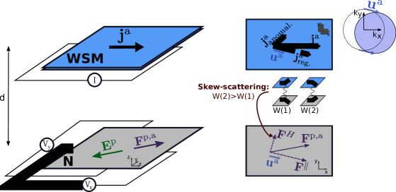
FIG. 1: Scheme of Coulomb drag between an active WSM layer and a passive normal metal layer (N). A current is driven through the active (top) layer and the resulting drag voltage is measured in the passive (bottom) layer. The electric current in the WSM is made of a regular and an anomalous part. The regular part corresponds to the shift of the Fermi-surface in the WSM, parametrized by the boost velocity $\boldsymbol{u}^{\textrm{a}}$. In the regime of low temperatures ($T\ll\min(v_{F}^{\textrm{a}},v_{F}^{\textrm{p}})/d$), symmetric (in the scattering angle) interlayer e-e collisions result in a drag force parallel to $\boldsymbol{u}^{a}$, while skew-scattering collisions result in a Hall drag force $\boldsymbol{F}^{H}$ which is perpendicular to $\boldsymbol{u}^{\textrm{a}}$. Hall voltage is induced in the passive layer due to the angles between $\boldsymbol{j}^{\textrm{a}}$ and $\boldsymbol{u}^{\textrm{a}}$ and between $\boldsymbol{F}^{\textrm{p,a}}$ and $\boldsymbol{u}^{\textrm{a}}$.

In a more technical sense, we can express the points mentioned above as follows. Due to the WSM spinor structure, the interlayer e-e scattering rate acquires a skew-scattering part. Schematically, a representative component of the skew-scattering rate is given by

$$W_{\boldsymbol{k},\boldsymbol{k}_{1}\rightarrow\boldsymbol{k}^{\prime},\boldsymbol{k}_{1^{\prime}}}^{\textrm{e-e [skew] (p,a)}}\sim\left(\boldsymbol{k}_{1}\times\boldsymbol{k}_{1^{\prime}}\right)\cdot\boldsymbol{M},$$ (10)

where $\boldsymbol{M}$ is a vector parametrizing the TRS-breaking in the WSM, $\boldsymbol{k},\boldsymbol{k}^{\prime}$ are the momenta of the passive layer electrons, and $\boldsymbol{k}_{1},\boldsymbol{k}_{1^{\prime}}$ are the momenta of the WSM electrons. This scattering process results in a drag force perpendicular to the boost velocity of the active layer,

$$\sum_{\boldsymbol{k}}\boldsymbol{k}I^{\textrm{e-e [skew] (p,a)}}\propto\eta_{H}^{D}\boldsymbol{u}^{\textrm{a}}\times\boldsymbol{M},$$ (11)

with $\eta_{H}^{D}$ being a drag coefficient in the transverse direction. This drag response from skew-scattering collisions resembles Hall viscosity [54, 55], with $\eta_{H}^{D}$ being an anti-symmetric part of a response tensor. We will thereby refer to this part of the friction as Hall friction.

In addition, the current in the WSM consists of both a regular and an anomalous part,

$$\boldsymbol{j}^{\textrm{a}}=\boldsymbol{j}_{\textrm{reg.}}^{\textrm{a}}+\boldsymbol{j}_{\textrm{anomal.}}^{\textrm{a}}.$$ (12)

The part $\boldsymbol{j}_{\textrm{reg.}}^{\textrm{a}}$ corresponds to the regular part of the velocity operator,

$$\boldsymbol{j}_{\textrm{reg.}}^{\textrm{a}}\equiv e\sum_{n,\boldsymbol{k}}f_{n\boldsymbol{k}}^{\textrm{a}}\boldsymbol{v}_{n\boldsymbol{k}}^{\textrm{a}}=e\sum_{n,\boldsymbol{k}}f_{n\boldsymbol{k}}^{\textrm{a}}\frac{\partial\epsilon_{n\boldsymbol{k}}^{\textrm{a}}}{\partial\boldsymbol{k}},$$ (13)

where $n$ denotes the band index. For a boosted velocity distribution, $\boldsymbol{j}_{\textrm{reg.}}^{\textrm{a}}$ is given by Eq. (4). The anomalous part of the current can be attributed to the off-diagonal (in band space) elements of the velocity operator. In the semiclassical language, these can be taken into account as corrections to the velocity operator from the Berry curvature and side jumps (known as intrinsic and extrinsic velocities, respectively [56]), such that (see Appendix C for more details)

$$\boldsymbol{j}_{\textrm{anomal.}}^{\textrm{a}}\equiv e\sum_{n,\boldsymbol{k}}f_{n\boldsymbol{k}}^{\textrm{a}}\left(\boldsymbol{v}_{n\boldsymbol{k}}^{\textrm{int.}}+\boldsymbol{v}_{n\boldsymbol{k}}^{\textrm{ext.}}\right).$$ (14)

Importantly, the intrinsic part of the current (corresponding to $\boldsymbol{v}_{n\boldsymbol{k}}^{\textrm{int.}}$) is a thermodynamic contribution which remains finite even in the absence of a Fermi-surface, as in the case of a Chern insulator [29]. On the other hand, Coulomb drag arises from real transitions on the Fermi surface due to e-e scattering, and thus vanishes in the presence of a gap [48].

We now proceed to the specific model and microscopic calculations.

III Model and outline of the calculation

III.1 The model

The non-interacting Hamiltonians of the layers are given by

$$H^{\textrm{a}} =\sum_{\xi=\pm 1}v_{F}\left(\xi\boldsymbol{\sigma}+C_{\xi}\hat{t}\right)\cdot\left(\boldsymbol{k}-\xi\frac{\boldsymbol{\Delta}_{k}}{2}\right)+V_{\textrm{imp}}^{\textrm{a}},$$ (15)

$$H^{\textrm{p}} =\frac{k^{2}}{2m}+V_{\textrm{imp}}^{\textrm{p}}.$$ (16)

The Weyl Hamiltonian consists of two tilted Weyl nodes with opposite chiralities $\xi=\pm 1$ separated in momentum space by $\boldsymbol{\Delta}_{k}$. The constants $C_{\xi}$ describe the tilt in the nodes, which is essential to break the TRS of the Fermi surface of a single node for a finite Hall drag. We consider $C_{\pm}=\pm C$ with $\left|C\right|<1$, for which the Weyl nodes are known as type-I [57]. For simplicity, we take $\hat{t}=\hat{\Delta}_{k}=\hat{z}$ with $\hat{z}$ being the axis perpendicular to the layers, so that the AHE in the WSM is in the x-y plane. Electrons in both layers are coupled via the Coulomb interaction, $H^{\textrm{e-e}}=\sum V_{\alpha\beta,\alpha^{\prime}\beta^{\prime}}^{\textrm{e-e},ll^{\prime}}c_{\alpha,l}^{\dagger}c_{\beta,l^{\prime}}^{\dagger}c_{\beta^{\prime}l^{\prime}}c_{\alpha^{\prime}l}$, where $l,l^{\prime}$ are layer indices and $\alpha,\alpha^{\prime},\beta,\beta^{\prime}$ represent the electron states. The disorder potential $V_{\textrm{imp}}^{l}$ in each layer is characterized by a scattering time $\tau^{l}$. In our analysis, we make the following assumptions:

• The interlayer distance and the momentum distance between the Weyl nodes satisfy $d\gg 1/\Delta_{k}$. In this regime, interlayer scattering involving internode transitions is negligible, and the total drag is a sum of contributions from the two independent Weyl nodes.

• The disorder potential in both layers is characterized by a Gaussian white-noise potential, with no correlation between the layers.

• The interlayer e-e scattering time is much longer than the momentum relaxation time due to the disorder.

• The interlayer distance is much smaller than the disorder mean free path of both layers, $d\ll v_{F}^{l}\tau^{l}$ with $v_{F}^{l}$ being the Fermi velocity of layer $l$ (the ballistic limit of the Coulomb drag).

• The thickness of the two layers is much smaller than the interlayer distance. In this limit, the Coulomb interaction simplifies to the Coulomb interaction between 2D layers [Eq. (52) in Appendix A].

• The thickness of the WSM is much larger than the interatomic distance, so that momentum sums in the z-axis can be approximated as integrals.

• Both layers are weakly interacting Fermi gases at the low temperature limit, i.e., $T\ll\epsilon_{F}^{l}$ ($\epsilon_{F}^{l}$ being the Fermi energy of layer $l$).

We now proceed to outline the computation of the drag conductivity in the model.

III.2 Outline of the microscopic calculation

First, we find the distribution function of the active WSM layer in the presence of an electric field $\boldsymbol{E}^{\textrm{a}}$, disregarding the interlayer e-e collisions. The solution of this problem (non-interacting AHE in the model of tilted WSM) is known [58, 59]. Here we compute the matrix (in band space) distribution function [60] via the Keldysh formalism (see Appendix A). The off-diagonal elements of the Keldysh distribution function of the WSM are small in the dimensionless parameter $1/\left(\epsilon_{F}^{\textrm{a}}\tau^{\textrm{a}}\right)$. This enables us to express the off-diagonal matrix elements in terms of the diagonal ones, and consequently to write the e-e collision integral as a functional of only the semiclassical distribution function $f_{n\boldsymbol{k}}^{\textrm{a}}$. Due to disorder skew scattering in the WSM, an electric field $\boldsymbol{E}^{\textrm{a}}$ shifts its Fermi surface in a direction rotated relative to the field. The correction to the distribution function, $\delta f_{n\boldsymbol{k}}^{\textrm{a}}\equiv f_{n\boldsymbol{k}}^{\textrm{a}}-f_{0}(\epsilon_{n\boldsymbol{k}}^{\textrm{a}})$, is given by

$$\delta f_{n\boldsymbol{k}}^{\textrm{a}}=-\frac{\partial f_{0}}{\partial\epsilon_{n\boldsymbol{k}}^{\textrm{a}}}\boldsymbol{v}_{n\boldsymbol{k}}^{\textrm{a}}\cdot\left(e\boldsymbol{E}^{\textrm{a}}+\frac{\tau_{n\boldsymbol{k},\parallel}^{\textrm{a}}}{\tau_{n\boldsymbol{k},\perp}^{\textrm{a}}}e\boldsymbol{E}^{\textrm{a}}\times\hat{z}\right)\tau_{n\boldsymbol{k},\parallel}^{\textrm{a}},$$ (17)

where $\tau_{\parallel}^{\textrm{a}}$ and $\tau_{\perp}^{\textrm{a}}$ are the momentum relaxation times in the directions parallel and perpendicular to the electric field (in our model $\tau_{\parallel}^{\textrm{a}}/\tau_{\perp}^{\textrm{a}}\ll 1$, see Appendix C for details). We note that $\delta f_{n\boldsymbol{k}}^{\textrm{a}}$ accounts for the entire non-equilibrium part of the distribution function, including the part known as the anomalous distribution arising from the side-jump correction to the disorder collision integral [44].

Having solved the distribution function in the active layer, we can now solve the Boltzmann equation for the passive layer [Eq. (1)] by substituting the active distribution function in the interlayer collision integral. Setting $\boldsymbol{E}^{\textrm{p}}=0$ in Eq. (1) for the calculation of the drag conductivity, the Boltzmann equation for the passive layer reads

$$0=I^{\textrm{e-e (p,a)}}\left[f^{\textrm{p}},f^{\textrm{a}}\right]+I^{\textrm{dis. (p)}}\left[f^{\textrm{p}}\right],$$ (18)

where we remind that $I^{\textrm{e-e (p,a)}}$ and $I^{\textrm{dis. (p)}}$ are the collision integrals due to interlayer e-e scattering and disorder scattering, respectively. Within the relaxation time approximation, the disorder collision integral in the passive layer is given by

$$I^{\textrm{dis. (p)}}\left[f^{\textrm{p}}\right]=-\frac{\delta f_{\boldsymbol{k}}^{\textrm{p}}}{\tau^{\textrm{p}}},$$ (19)

where $\delta f_{\boldsymbol{k}}^{\textrm{p}}\equiv f_{\boldsymbol{k}}^{\textrm{p}}-f_{0}(\epsilon_{\boldsymbol{k}}^{\textrm{p}})$ is the non-equilibrium part of the distribution function in the passive layer. The interlayer e-e collision integral is given by

$$I_{\boldsymbol{k}}^{\textrm{e-e (p,a)}}\left[f^{\textrm{p}},f^{\textrm{a}}\right] =-W\sum_{\xi=\pm 1}\sum_{n_{1},n_{1^{\prime}}}\intop_{\boldsymbol{k}^{\prime},\boldsymbol{k}_{1},\boldsymbol{k}_{1^{\prime}}}[w_{\boldsymbol{k},n_{1}\boldsymbol{k}_{1}\rightarrow\boldsymbol{k}^{\prime},n_{1^{\prime}}\boldsymbol{k}_{1^{\prime}}}^{\textrm{e-e}}f_{\boldsymbol{k}}^{\textrm{p}}f_{n_{1}\boldsymbol{k}_{1}}^{\textrm{a}}\left(1-f_{\boldsymbol{k}^{\prime}}^{\textrm{p}}\right)\left(1-f_{n_{1^{\prime}}\boldsymbol{k}_{1^{\prime}}}^{\textrm{a}}\right)$$

$$-w_{\boldsymbol{k}^{\prime},n_{1^{\prime}}\boldsymbol{k}_{1^{\prime}}\rightarrow\boldsymbol{k},n_{1}\boldsymbol{k}_{1}}^{\textrm{e-e}}f_{\boldsymbol{k}^{\prime}}^{\textrm{p}}f_{n_{1^{\prime}}\boldsymbol{k}_{1^{\prime}}}^{\textrm{a}}\left(1-f_{\boldsymbol{k}}^{\textrm{p}}\right)\left(1-f_{n_{1}\boldsymbol{k}_{1}}^{\textrm{a}}\right)].$$ (20)

Here, we denote $\intop_{\boldsymbol{k}}\equiv\intop d\boldsymbol{k}/\left(2\pi\right)^{d}$ for the momentum integrations ($d=2,3$ for the metal and the WSM layers, respectively). We omit the Weyl node index $\xi$ for objects in the integrand, recalling that we neglect internode scattering. Since disorder scattering is the dominant momentum relaxation mechanism in the passive layer, one may replace $f_{\boldsymbol{k}}^{\textrm{p}}\rightarrow f_{0}(\epsilon_{\boldsymbol{k}}^{\textrm{p}})$ in the interlayer collision integral [Eq. (20)], making it a functional of only the active distribution function, $I_{\boldsymbol{k}}^{\textrm{e-e (p,a)}}\left[f^{\textrm{a}}\right]\equiv I_{\boldsymbol{k}}^{\textrm{e-e (p,a)}}\left[f_{\boldsymbol{k}}^{\textrm{p}}=f_{0}(\epsilon_{\boldsymbol{k}}^{\textrm{p}}),f^{\textrm{a}}\right]$. The factor $W$ (the WSM layer’s thickness) in Eq. (20) is due the quasi-2D nature of the interlayer scattering (see Appendix A).

Note that although the collision integral in Eq. (20) looks like a standard e-e collision integral, this is not the case. The complexity is hidden in the interlayer scattering rate $w_{\boldsymbol{k},n_{1}\boldsymbol{k}_{1}\rightarrow\boldsymbol{k}^{\prime},n_{1^{\prime}}\boldsymbol{k}_{1^{\prime}}}^{\textrm{e-e}}$, which is computed taking into account virtual transitions in the WSM (see Appendix A for more details). Such processes are crucial for the Coulomb Hall drag. Among such processes is the interference between interlayer e-e scattering and intermediate disorder scattering, breaking the momentum conservation of the incoming and outgoing electrons. Therefore, one cannot assume $\boldsymbol{k}_{1}+\boldsymbol{k}=\boldsymbol{k}^{\prime}+\boldsymbol{k}_{1^{\prime}}$ in the integrand of Eq. (20) as is usually the case.

Substituting Eq. (19) into Eq. (18), one finds

$$\delta f_{\boldsymbol{k}}^{\textrm{p}}=\tau^{\textrm{p}}I_{\boldsymbol{k}}^{\textrm{e-e (p,a)}}\left[f^{\textrm{a}}\right].$$ (21)

Employing Eq. (21), one finds electric current in the passive layer

$$\boldsymbol{j}^{\textrm{p}}=e\intop_{\boldsymbol{k}}\boldsymbol{v}_{\boldsymbol{k}}^{\textrm{p}}\delta f_{\boldsymbol{k}}^{\textrm{p}}.$$ (22)

The drag conductivity is given by

$$\sigma_{\alpha\beta}^{D}\equiv\frac{j_{\alpha}^{\textrm{p}}}{E_{\beta}^{\textrm{a}}}.$$ (23)

For a passive layer with a parabolic spectrum and within the relaxation time approximation, one can relate the drag current to the drag force (or, momentum transfer rate between the layers) $\boldsymbol{F}^{\textrm{p,a}}\equiv\intop_{\boldsymbol{k}}\boldsymbol{k}I_{\boldsymbol{k}}^{\textrm{e-e (p,a)}}$. Employing Eqs. (21) and (22), one finds

$$\boldsymbol{j}^{\textrm{p}}=\frac{e\tau^{\textrm{p}}}{m}\boldsymbol{F}^{\textrm{p,a}}\left[f^{\textrm{a}}\right].$$ (24)

Thinking of the Coulomb drag in terms of forces gives additional insight. In the experimentally prevalent regime of low temperatures ($T\ll T_{d}$, with $T_{d}\equiv\min\left(v_{F}^{\textrm{a}},v_{F}^{\textrm{p}}\right)/d$), the Hall drag conductivity can be divided into two parts:

1. Parallel friction: Drag force $\boldsymbol{F}^{\textrm{p,a}}$ which is parallel to the Fermi surface shift in the active layer. Because an electric field $\boldsymbol{E}^{\textrm{a}}$ in the WSM layer creates a perpendicular component to the Fermi surface shift due to skew scattering in the WSM [second term in Eq. (17)], parallel friction creates a corresponding component in the passive layer current which is perpendicular to $\boldsymbol{E}^{\textrm{a}}$, i.e., Hall drag current.

2. Hall friction: Drag force $\boldsymbol{F}^{\textrm{p,a}}$ which is perpendicular to the Fermi surface shift in the active layer. This part of the drag arises due to the many-body skew-scattering part of the interlayer collision integral.

In the opposite regime of high temperatures ($T\gg T_{d}$), the picture is complicated by the energy dependence of the Fermi-surface shift in the active layer [Eq. (17)]. In this case, the drag force can be decomposed into three components: parallel and perpendicular to the Fermi-surface shift as in the previous case, as well as a component related to the energy dependence of the Fermi-surface shift. In this case, even on the level of a simple interlayer collision integral (disregarding the interlayer skew-scattering part), the drag force $\boldsymbol{F}^{\textrm{p,a}}$ is generally not parallel to the Fermi surface shift.

Having outlined the main steps of the calculation, we now turn to the computation of the drag conductivity and resistivity.

IV Results: drag conductivity and resistivity

First we present the interlayer e-e collision integral in more detail, introducing its skew-scattering part.

IV.1 Interlayer e-e collision integral

The collision integral can be written in the general form of Eq. (20), with the interlayer e-e scattering rate separated into contributions from three different processes,

$$w_{\boldsymbol{k},n_{1}\boldsymbol{k}_{1}\rightarrow\boldsymbol{k}^{\prime},n_{1^{\prime}}\boldsymbol{k}_{1^{\prime}}}^{\textrm{e-e}}=w_{\boldsymbol{k},n_{1}\boldsymbol{k}_{1}\rightarrow\boldsymbol{k}^{\prime},n_{1^{\prime}}\boldsymbol{k}_{1^{\prime}}}^{\textrm{Born}}+w_{\boldsymbol{k},n_{1}\boldsymbol{k}_{1}\rightarrow\boldsymbol{k}^{\prime},n_{1^{\prime}}\boldsymbol{k}_{1^{\prime}}}^{\textrm{s.j.}}+w_{\boldsymbol{k},n_{1}\boldsymbol{k}_{1}\rightarrow\boldsymbol{k}^{\prime},n_{1^{\prime}}\boldsymbol{k}_{1^{\prime}}}^{\textrm{{e-e-imp}}}.$$ (25)

The term $w^{\textrm{Born}}$ refers to the part calculated on the level of the Born approximation within the RPA (random-phase approximation) approach, resulting in a rate proportional to the square of the screened Coulomb potential [Eq. (84) in the Appendix]. It is an even function of the angle between the momenta of the scattering electrons in the WSM. Although it is the largest scattering amplitude, the two other scattering processes are of equal importance to Hall drag, since they give rise to interlayer skew scattering. The term $w^{\textrm{s.j.}}$ corresponds to a correction due to side jumps of the WSM electrons; $w^{\textrm{{e-e-imp}}}$ corresponds to interference between e-e scattering and e-impurity scattering in the WSM. These scattering rates are calculated using the Keldysh formalism, accounting for processes involving virtual transitions in the WSM layer. The virtual transitions correspond to interband elements of the matrix Green functions. The full expressions for these rates are presented in Appendix A [Eq. (93) for $w^{\textrm{s.j.}}$ and Eq. (100) for $w^{\textrm{{e-e-imp}}}$]. We now briefly describe the physical processes giving rise to the skew-scattering terms.

The side-jump process modifies the interlayer e-e collision integral in an analogous way to how it modifies the electron-disorder collision integral [43]. In the context of interlayer e-e scattering, a WSM electron acquires a coordinate shift when it scatters from the incoming to the outgoing state (thus, “side jump”). In the presence of an external field, this coordinate shift changes the electric potential energy of the electron. Therefore, the energy conservation condition for the e-e scattering process is modified. Consequently, the side-jump scattering rate $w^{\textrm{s.j.}}$ is proportional to the applied electric field ${\bf E}^{\textrm{a}}$, and scales linearly with it in the low field limit. Therefore, on the level of the linear response, one replaces the distribution functions in Eq. (20) with their equilibrium values, $f_{n\boldsymbol{k}}^{\textrm{a}}\rightarrow f_{0}(\epsilon_{n\boldsymbol{k}}^{\textrm{a}})$. Even in this approximation of equilibrium distribution functions, the side-jump scattering rate results in a finite contribution to the collision integral.

Next we discuss the last term in Eq. (25), $w_{\boldsymbol{k},n_{1}\boldsymbol{k}_{1}\rightarrow\boldsymbol{k}^{\prime},n_{1^{\prime}}\boldsymbol{k}_{1^{\prime}}}^{\textrm{{e-e-imp}}}$. It involves scattering through an intermediate state, and is proportional to the complex phase of the Bloch wavefunctions acquired during this scattering. Because this term involves both e-e and disorder scattering, it does not conserve the total electron momenta, unlike the other scattering processes discussed above, which are proportional to the delta function $\delta_{\boldsymbol{k}+\boldsymbol{k}_{1}-\boldsymbol{k}^{\prime}-\boldsymbol{k}_{1^{\prime}}}$.

We now move on to the calculation of the drag conductivities.

IV.2 Drag conductivity

For the clarity of computation, we focus on two limiting cases: low temperatures ($T\ll T_{d}$) and high temperatures ($T\gg T_{d}$) (we remind the reader the definition $T_{d}\equiv\min\left(v_{F}^{\textrm{a}},v_{F}^{\textrm{p}}\right)/d$).

IV.2.1 Low temperatures

In the regime of low temperatures ($T\ll T_{d}$), the distribution function $\delta f_{n\boldsymbol{k}}^{\textrm{a}}$ [Eq. (17)] can be approximated by a boosted velocity distribution [Eq. (2)]. This is done by replacing $\boldsymbol{v}_{n\boldsymbol{k}}^{\textrm{a}}\approx\left(v_{F}^{\textrm{a}}\right)^{2}\boldsymbol{k}/\epsilon_{F}^{\textrm{a}}$ (this misses a term in the z-component of $\boldsymbol{v}_{n\boldsymbol{k}}^{\textrm{a}}$, but we are interested in the components in the x-y plane) and neglecting the energy dependence of the relaxation times. These approximations are justified since the particle-hole scattering is predominantly perpendicular in both layers [i.e., $\boldsymbol{q}\perp\boldsymbol{v}_{\boldsymbol{k}}$ where $\boldsymbol{q}$ is the momentum exchange in the collision and $\boldsymbol{v}_{\boldsymbol{k}}$ is the electron velocity, making the collision quasi-elastic. For a detailed discussion, see the text following Eq. (118) of the Appendix]. This accuracy is sufficient to account for the leading part of the drag conductivities in the small parameter $T/T_{d}$. We introduce the parametrization

$$\delta f_{n\boldsymbol{k}}^{\textrm{a}}=-T\frac{\partial f_{0}(\epsilon_{n\boldsymbol{k}}^{\textrm{a}})}{\partial\epsilon_{n\boldsymbol{k}}^{\textrm{a}}}g_{n\boldsymbol{k}}^{\textrm{a}}.$$ (26)

After substituting Eq. (26) in Eq. (17), one finds

$$g_{n\boldsymbol{k}}^{\textrm{a}}=\frac{\boldsymbol{k}\cdot\boldsymbol{u}^{\textrm{a}}}{T},$$ (27)

where $\boldsymbol{u}^{\textrm{a}}$ is the boost velocity in the active layer, given by

$$u_{\alpha}^{\textrm{a}}=\frac{\left(v_{F}^{\textrm{a}}\right)^{2}\tau_{\parallel}^{\textrm{a}}}{\epsilon_{F}^{\textrm{a}}}\left(\delta_{\alpha\beta}+\epsilon_{\alpha\beta}\frac{\tau_{\parallel}^{\textrm{a}}}{\tau_{\perp}^{\textrm{a}}}\right)eE_{\beta}^{\textrm{a}}.$$ (28)

Here, the momentum relaxation times $\tau_{\parallel}^{\textrm{a}},\tau_{\perp}^{\textrm{a}}$ are computed at the Fermi energy (see Appendix C). We now substitute the distribution function in the active layer with the non-equilibrium part given by Eq. (26) into the interlayer e-e collision integral [Eq. $(\ref{eq:general coll integral}$) with the scattering rates given in Eq. (25)] , and derive the linearized interlayer collision integral

$${\cal I}_{\boldsymbol{k}}^{\textrm{e-e (p,a)}} =-\frac{W}{T}\sum_{\xi=\pm 1}\sum_{n_{1},n_{1^{\prime}}}\intop_{\boldsymbol{q},\boldsymbol{k}_{1},\boldsymbol{k}_{1^{\prime}}}f_{0}(\epsilon_{\boldsymbol{k}}^{\textrm{p}})f_{0}(\epsilon_{n_{1}\boldsymbol{k}_{1}}^{\textrm{a}})\left(1-f_{0}(\epsilon_{\boldsymbol{k}+\boldsymbol{q}}^{\textrm{p}})\right)\left(1-f_{0}(\epsilon_{n_{1^{\prime}}\boldsymbol{k}_{1^{\prime}}}^{\textrm{a}})\right)$$

$$\times\left[w_{\boldsymbol{k},n_{1}\boldsymbol{k}_{1}\rightarrow\boldsymbol{k}+\boldsymbol{q},n_{1^{\prime}}\boldsymbol{k}_{1^{\prime}}}^{\textrm{Born}}\boldsymbol{q}\cdot\boldsymbol{u}^{\textrm{a}}+w_{\boldsymbol{k},n_{1}\boldsymbol{k}_{1}\rightarrow\boldsymbol{k}+\boldsymbol{q},n_{1^{\prime}}\boldsymbol{k}_{1^{\prime}}}^{\textrm{{e-e-imp}}}\left(\boldsymbol{k}_{1}-\boldsymbol{k}_{1^{\prime}}\right)\cdot\boldsymbol{u}^{\textrm{a}}+2w_{\boldsymbol{k},n_{1}\boldsymbol{k}_{1}\rightarrow\boldsymbol{k}+\boldsymbol{q},n_{1^{\prime}}\boldsymbol{k}_{1^{\prime}}}^{\textrm{s.j.}}T\right].$$ (29)

Here, we utilized the momentum conservation of the process corresponding to $w^{\textrm{Born}}$, forcing $\boldsymbol{k}_{1^{\prime}}=\boldsymbol{k}_{1}-\boldsymbol{q}$ in this term.

We now calculate the drag force $\boldsymbol{F}^{\textrm{p,a}}$ between the layers by substituting Eq. (29) into Eq. (6). The resulting drag force can be written as a linear response to the boost velocity in the active layer. We identify the generation of diagonal and Hall-like responses, writing

$$F_{\alpha}^{\textrm{p,a}}=\left(\delta_{\alpha\beta}\eta_{\parallel}^{D}+\epsilon_{\alpha\beta}\eta_{H}^{D}\right)\frac{u_{\beta}^{\textrm{a}}}{d}.$$ (30)

Here, the diagonal response $\eta_{\parallel}^{D}$ is generated by the Born-approximation part of the collision integral, and the Hall-like response $\eta_{H}^{D}$ comes from the many-body skew-scattering processes corresponding to e-e-impurity interference and side jumps. Calculation of the momentum transfer with the total interlayer scattering rate (see Appendix B) yields

$$\eta_{\parallel}^{D} =\frac{\pi\zeta(3)}{32}\frac{T^{2}}{v_{F}^{\textrm{a}}v_{F}^{\textrm{p}}\kappa^{\textrm{a}}\kappa^{\textrm{p}}d^{3}},$$ (31)

$$\eta_{H}^{D} =-\frac{C}{2\epsilon_{F}^{\textrm{a}}\tau^{\textrm{a}}}\eta_{\parallel}^{D}.$$ (32)

Here, $\zeta(z)$ is the Riemann Zeta function, and $\kappa^{l}=2\pi e^{2}\nu_{2d}^{l}/\epsilon_{r}$ is the Thomas-Fermi wavevector of layer $l$ with 2D density of states $\nu_{2d}^{l}$ ($\nu_{2d}^{\textrm{p}}\equiv\nu^{\textrm{p}}$ for the metal layer and $\nu_{2d}^{\textrm{a}}\equiv\nu^{\textrm{a}}W$ for the WSM layer) and dielectric constant $\epsilon_{r}$. We have thus found the dependence of the drag force on the active layer boost velocity. One can readily find the drag force $\boldsymbol{F}^{\textrm{p,a}}$ as a function of the electric field in the active layer by substituting Eq. (28) into Eq. (30). The dragged current is proportional to the drag force [Eq. (24)]. Employing Eq. (23), one finds the drag conductivity. For the longitudinal component, one finds

$$\sigma_{xx}^{D}=e^{2}\frac{\ell^{\textrm{a}}\ell^{\textrm{p}}}{k_{F}^{\textrm{a}}k_{F}^{\textrm{p}}}\frac{\eta_{\parallel}^{D}}{d}=e^{2}\frac{\pi\zeta(3)}{64}\frac{T^{2}}{\epsilon_{F}^{\textrm{a}}\epsilon_{F}^{\textrm{p}}}\frac{\ell^{\textrm{a}}\ell^{\textrm{p}}}{\kappa^{\textrm{a}}\kappa^{\textrm{p}}d^{4}},$$ (33)

where $\ell^{l}\equiv v_{F}^{l}\tau_{\parallel}^{l}$ is the mean free path in layer $l$ (for the passive layer, $\tau_{\parallel}^{\textrm{p}}=\tau^{\textrm{p}})$. The result for the longitudinal drag conductivity differs from that of the drag between two 2D metals [25] by a numerical factor due to the dimensionality of the WSM layer.

Next we discuss the Hall drag conductivity. Since the boost velocity in the active layer is rotated relative to the electric field, a corresponding Hall current is dragged in the passive layer by the parallel friction. Denoting the corresponding contribution to the Hall drag conductivity by $\sigma_{xy}^{D[\eta_{\parallel}^{D}]}$, one finds

$$\sigma_{xy}^{D[\eta_{\parallel}^{D}]}=\frac{\tau_{\parallel}^{\textrm{a}}}{\tau_{\perp}^{\textrm{a}}}\sigma_{xx}^{D}=\frac{3C}{2\epsilon_{F}^{\textrm{a}}\tau^{\textrm{a}}}\sigma_{xx}^{D}.$$ (34)

The Hall friction gives rise to a force $F_{\alpha}^{H}\equiv\epsilon_{\alpha\beta}\eta_{H}^{D}u_{\beta}^{\textrm{a}}/d$ perpendicular to the boost velocity. This results in an additional contribution to the Hall drag conductivity

$$\sigma_{xy}^{D[\eta_{H}^{D}]}=e^{2}\frac{\ell^{\textrm{a}}\ell^{\textrm{p}}}{k_{F}^{\textrm{a}}k_{F}^{\textrm{p}}}\frac{\eta_{H}^{D}}{d}.$$ (35)

Substituting the value of the Hall response coefficient $\eta_{H}^{D}$, one gets

$$\sigma_{xy}^{D[\eta_{H}^{D}]}=-\frac{C}{2\epsilon_{F}^{\textrm{a}}\tau^{\textrm{a}}}\sigma_{xx}^{D}.$$ (36)

The total Hall drag conductivity is additive in the contributions,

$$\sigma_{xy}^{D}=\sigma_{xy}^{D[\eta_{\parallel}^{D}]}+\sigma_{xy}^{D[\eta_{H}^{D}]}=\frac{C}{\epsilon_{F}^{\textrm{a}}\tau^{\textrm{a}}}\sigma_{xx}^{D}.$$ (37)

The ratio $\sigma_{xy}^{D}/\sigma_{xx}^{D}\simeq C/\left(\epsilon_{F}^{\textrm{a}}\tau^{\textrm{a}}\right)$ is parametrically equal to the ratio between the Fermi-surface contribution of the Hall conductivity and the longitudinal conductivity in the non-interacting WSM. Note that unlike the anomalous Hall conductivity, which has an intrinsic contribution proportional to the momentum distance between the Weyl nodes ($\sigma_{xy}^{\textrm{int}}\sim\Delta_{k}$), the Hall drag conductivity has no bulk contribution [48, 49].

IV.2.2 High temperatures

In the high-temperature limit ($T\gg T_{d}$), an additional complication arises due to the deviation of the distribution function in the active layer [Eq. (17)] from a boosted velocity distribution. This deviation is due to the non-parabolic spectrum of the WSM and the energy dependence of the relaxation times. In this case, one needs to replace Eq. (27) with an “energy-dependent boost velocity” ansatz,

$$g_{n\boldsymbol{k}}^{\textrm{a}}=\frac{\boldsymbol{k}\cdot\boldsymbol{u}^{\textrm{a}}(\epsilon_{n\boldsymbol{k}}^{\textrm{a}})}{T},$$ (38)

where $\boldsymbol{u}^{\textrm{a}}(\epsilon)$ is a boost velocity at a given energy, analogous to Eq. (28) evaluated at energy $\epsilon$,

$$u_{\alpha}^{\textrm{a}}(\epsilon)=\frac{\left(v_{F}^{\textrm{a}}\right)^{2}\tau_{\parallel}^{\textrm{a}}(\epsilon)}{\epsilon}\left(\delta_{\alpha\beta}+\epsilon_{\alpha\beta}\frac{\tau_{\parallel}^{\textrm{a}}(\epsilon)}{\tau_{\perp}^{\textrm{a}}(\epsilon)}\right)eE_{\beta}^{\textrm{a}}.$$ (39)

Note that we have neglected the anisotropy in the WSM by approximating $\boldsymbol{u}^{\textrm{a}}(\epsilon,\hat{k})\sim\boldsymbol{u}^{\textrm{a}}(\epsilon)$, taking into account the leading order in the tilt parameter $C$.

By calculating the momentum transfer from the interlayer e-e collision integral as in the previous section, we now find the drag force

$$F_{\alpha}^{\textrm{p,a}}=\left(\delta_{\alpha\beta}\eta_{\parallel(0)}^{D}+\epsilon_{\alpha\beta}\eta_{H}^{D}\right)\frac{u_{\beta}^{\textrm{a}}}{d}+\delta_{\alpha\beta}\eta_{\parallel(1)}^{D}\frac{\epsilon_{F}^{\textrm{a}}}{d}\left.\frac{\partial u_{\beta}^{\textrm{a}}(\epsilon)}{\partial\epsilon}\right|_{\epsilon=\epsilon_{F}^{\textrm{a}}}.$$ (40)

The terms $\eta_{\parallel(0)}^{D}$ and $\eta_{H}^{D}$ correspond respectively to the Born-approximation and skew-scattering rates as in the previous case ($\eta_{\parallel(0)}^{D}$ has the same meaning as the non-indexed $\eta_{\parallel}^{D}$ in the previous section). In addition, there is a term proportional to the energy derivative of the active layer’s boost velocity, which was not present in the previous case. This term arises even within the Born-approximation part of the interlayer collision integral. Generally, the vector $\left[\partial\boldsymbol{u}^{\textrm{a}}(\epsilon)/\partial\epsilon\right]_{\epsilon=\epsilon_{F}^{\textrm{a}}}$ is not parallel to $\boldsymbol{u}^{\textrm{a}}$, and therefore even in the Born-approximation level, the interlayer collision integral generates momentum transfer perpendicular to $\boldsymbol{u}^{\textrm{a}}$. The drag coefficients in the high-temperature and small-tilt ($C\ll 1$) limits are given by

$$\eta_{\parallel(0)}^{D} =\bar{\eta}Q_{1}(\frac{v_{F}^{\textrm{p}}}{v_{F}^{\textrm{a}}}),$$ (41)

$$\eta_{\parallel(1)}^{D} =\bar{\eta}Q_{2}(\frac{v_{F}^{\textrm{p}}}{v_{F}^{\textrm{a}}})\times\min\left[1,\left(\frac{v_{F}^{\textrm{p}}}{v_{F}^{\textrm{a}}}\right)^{2}\right],$$ (42)

$$\eta_{H}^{D} =-\frac{C}{2\epsilon_{F}^{\textrm{a}}\tau^{\textrm{a}}}\bar{\eta}Q_{3}(\frac{v_{F}^{\textrm{p}}}{v_{F}^{\textrm{a}}}),$$ (43)

where we defined

$$\bar{\eta}^{D}\equiv\frac{\pi^{3}}{480}\frac{T_{d}T}{v_{F}^{\textrm{a}}v_{F}^{\textrm{p}}\kappa^{\textrm{a}}\kappa^{\textrm{p}}d^{3}},$$ (44)

and $Q_{1,2,3}(z)$ are factors of order one given in the Appendix [Eqs. (130)-(132)]. Note that $\eta_{\parallel(1)}^{D}$ [the drag coefficient multiplying $\partial\boldsymbol{u}^{\textrm{a}}(\epsilon)/\partial\epsilon$] is suppressed in the limit $v_{F}^{\textrm{p}}/v_{F}^{\textrm{a}}\ll 1$. This comes from the phase-space restrictions of the interlayer e-e scattering. The particle-hole pairs in both layers have to satisfy $\boldsymbol{v}_{F}^{l}\cdot\boldsymbol{q}=\omega$, with $\omega$ being the energy transfer in the collision. In the case $v_{F}^{\textrm{p}}/v_{F}^{\textrm{a}}\ll 1$, forward scattering is suppressed in the WSM (i.e., scattering with $\boldsymbol{q}$ parallel to the velocity of the WSM electron $\boldsymbol{v}_{\boldsymbol{k}_{1}}^{\textrm{a }}$). Thus, the effect of the energy dependence of the boost velocity on the drag is negligible in this limit.

It is reasonable to assume that the typical energy dependence of the transport times in realistic materials is a power-law function. Consequently, the boost velocity has a power-law energy dependence [see Eq. (39)]. Generally, the parallel and perpendicular (relative to the electric field) components of the boost velocity may have different scaling with energy. We denote these components [first and second terms in Eq. (39)] as $u_{\parallel}^{\textrm{a}}(\epsilon)\sim\epsilon^{b_{\parallel}}$ and $u_{\perp}^{\textrm{a}}(\epsilon)\sim\epsilon^{b_{\perp}}$. The drag conductivities are given by

$$\sigma_{xx}^{D} =e^{2}\frac{\ell^{\textrm{a}}\ell^{\textrm{p}}}{k_{F}^{\textrm{a}}k_{F}^{\textrm{p}}d}\left(\eta_{\parallel(0)}^{D}+b_{\parallel}\eta_{\parallel(1)}^{D}\right),$$ (45)

$$\sigma_{xy}^{D[\eta_{\parallel}^{D}]} =e^{2}\frac{\ell^{\textrm{a}}\ell^{\textrm{p}}}{k_{F}^{\textrm{a}}k_{F}^{\textrm{p}}d}\frac{\tau_{\parallel}^{\textrm{a}}}{\tau_{\perp}^{\textrm{a}}}\left(\eta_{\parallel(0)}^{D}+b_{\perp}\eta_{\parallel(1)}^{D}\right),$$ (46)

and $\sigma_{xy}^{D[\eta_{H}^{D}]}$ still given by Eq. (35). In our model, $b_{\parallel}=-3$ and $b_{\perp}=-2$. Thus, the drag force computed within the Born approximation [the terms accounted by $\eta_{\parallel(0)}^{D}$ and $\eta_{\parallel(1)}^{D}$ in Eq. (40)] in our model is indeed not parallel to $\boldsymbol{u}^{\textrm{a}}$.

Since $b_{\parallel}$ and $b_{\perp}$ are negative, the two terms in both Eqs. (45) and (46) are of opposite sign. Depending on the numerical prefactors, this may result in an opposite sign for the drag conductivities in the two limits of $T\ll T_{d}$ and $T\gg T_{d}$, and thus lead to a non-monotonous temperature dependence. Physically, the non-monotonous behavior can be understood as follows. When $u_{\alpha}^{\textrm{a}}(\epsilon)$ is a decreasing function of the energy, quasi-elastic and forward (strongly inelastic) interlayer scattering processes give opposite contributions to the drag force $F_{\alpha}^{\textrm{p,a}}$. Since forward scattering gives a significant contribution only for temperatures $T\gtrsim T_{d}$, a non-monotonous temperature dependence of the drag conductivities may arise. The quasi-elastic contribution to the drag is conventional, and its direction depends on the signs of the curvatures of the single-particle spectrum in the layers [7]. The sign of the contribution due to forward scattering is controlled by the energy dependence of $u_{\alpha}^{\textrm{a}}(\epsilon)$, quantified by the coefficients $b_{\parallel}$ and $b_{\perp}$ [these are related to the transport times, see Eq. (38)]. We note that the scenario where forward and quasi-elastic interlayer scattering contribute to the drag in opposite directions is quite general. It is expected to occur in a generic Coulomb drag setup, provided that scattering time in one of the layers is a decreasing function of energy. In the case where both layers have energy-dependent scattering times, the behavior is more complicated, since forward scattering can be more dominant in one layer than in the other depending on the spectrum of the two layers. For a scattering event in which both electrons in the two layers scatter in the forward direction, the sign of the resulting contribution to the drag also depends on the product of the derivatives $\partial\tau^{l}(\epsilon)/\partial\epsilon$. For two identical layers, both scattering mechanisms contribute positively to the drag conductivity. Thus, the two layers being different is essential for a non-monotonous temperature dependence of the drag.

To summarize, on a qualitative level, the direction of the drag is controlled by two independent mechanisms: (i) the curvatures of the single-particle spectrum in two layers; (ii) the direction in which the momentum relaxation rate $\tau(\epsilon)$ changes with energy. The effect (ii) is pronounced only when the temperature is not too low ($T\gtrsim T_{d}$).

Finally, we numerically calculate the longitudinal and Hall drag conductivities in the entire temperature range, and present the results in Fig. 2(a-b),(d-e). For the calculation, we restore physical units and use realistic parameters for the TRS-breaking WSM $\textrm{Co}_{\textrm{3}}\textrm{Sn}_{\textrm{2}}\textrm{S}_{\textrm{2}}$ [63, 64, 65] and GaAs [66] as the layers. The non-monotonous temperature dependence of $\sigma_{xx}^{D}$ can be seen from the plots, showing maxima at $T\sim T_{d}$ [Figs. 2(a,d)].

We note that within the analytic approximation for the coefficients $\eta_{\parallel(0)}^{D}$ and $\eta_{\parallel(1)}^{D}$ at $T\gg T_{d}$ [Eqs. (41), (42)], the two terms in $\sigma_{xx}^{D}$ [Eq. (45)] nearly cancel, but their sum is still an increasing function of $T$. This analytic approximation takes the Coulomb interaction in the limits $T\ll\epsilon_{F}^{\textrm{a}},\epsilon_{F}^{\textrm{p}}$, zero tilt for the WSM, and Thomas-Fermi screening lengths ($1/\kappa^{l}$) much shorter than the interlayer distance $d$. The small but finite deviations from these limits in the numerical calculation enhance the negative $\sim\eta_{\parallel(1)}^{D}$ term due to a reduction in the screening at frequencies $\omega\sim T_{d}$, and consequently result in $\sigma_{xx}^{D}$ being a decreasing function of temperature at $T\gtrsim T_{d}$.

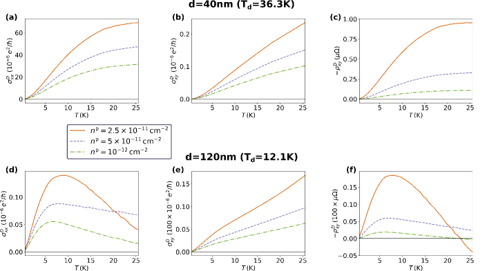
FIG. 2: Drag conductivity and resistivity from numerical calculation of the interlayer collision integral [Eq. (20)] as a function of temperature, for interlayer distance $d=\textrm{40}\textrm{nm}$ (a-c) and $d=120\textrm{nm}$ (d-f). (a), (d) Longitudinal drag conductivity. (b), (e) Hall drag conductivity. (c), (f) Hall drag resistivity. WSM is taken as a single pair of Weyl nodes, with $\epsilon_{F}^{\textrm{a}}=60\rm{meV}$, $v_{F}^{\textrm{a}}=1.9\times 10^{5}\rm{m}/\rm{s}$, $\tau^{\textrm{a}}=2\times 10^{-12}\rm{s}$, internode distance $\Delta_{k}=4.7\textrm{nm}^{-1}$, tilt parameter $C=0.3$ and thickness $W=15\rm{nm}$. The metal consists of one electronic band with $m=0.067m_{e}$ ($m_{e}$ being the electron mass), $\tau^{\textrm{p}}=2\times 10^{-11}\rm{s}$ and varying carrier densities $n^{\textrm{p}}$ as given in the legend at the center of the figure. Dielectric constant is $\epsilon_{r}=12$.

IV.3 Drag resistivity

We now turn to the drag resistivities, which are defined by $\rho_{\alpha\beta}^{D}\equiv-E_{\alpha}^{\textrm{p}}/j_{\beta}^{\textrm{a}}$ (the minus sign is conventional). We compute these by inverting the generalized conductivity tensor $\sigma_{\alpha\beta}^{l,l^{\prime}}\equiv j_{\alpha}^{l}/E_{\beta}^{l^{\prime}}$ [for convenience, in this section we consider the sheet (2D) conductivities and currents of the WSM layer, obtained by multiplying the bulk 3D quantities by the layer thickness]. Focusing on the components $\alpha,\beta\in\left\{x,y\right\}$, $\sigma_{\alpha\beta}^{l,l^{\prime}}$ can be viewed as $4\times 4$ tensor. In these notations, $\sigma_{\alpha\beta}^{\textrm{p,a}}=\sigma_{\alpha\beta}^{D}$ is the drag conductivity and $\sigma_{\alpha\beta}^{l,l}$ is the non-interacting conductivity of layer $l$. In the leading order in the small parameter $\left(\sigma_{xx}^{D}\right)^{2}/\left(\sigma_{xx}^{\textrm{a}}\sigma_{xx}^{\textrm{p}}\right)$, one finds

$$\rho_{xx}^{D} =\rho_{xx}^{\textrm{p}}\rho_{xx}^{\textrm{a}}\sigma_{xx}^{D},$$ (47)

$$\rho_{xy}^{D} =\rho_{xx}^{D}\left(\frac{\sigma_{xy}^{D}}{\sigma_{xx}^{D}}-\frac{\sigma_{xy}^{\textrm{a}}}{\sigma_{xx}^{\textrm{a}}}\right),$$ (48)

where $\rho_{xx}^{l}$ is the longitudinal (2D) resistivity of layer $l$. We now analyze these results for the cases of low and high-temperature regimes.

IV.3.1 Low temperatures

For low temperatures ($T\ll T_{d}$), the longitudinal drag resistivity [Eq. (47)] is given by

$$\rho_{xx}^{D}=\frac{\eta_{\parallel}^{D}}{e^{2}n^{\textrm{a}}n^{\textrm{p}}d},$$ (49)

where $n^{\textrm{a}}$ and $n^{\textrm{p}}$ are the (2D) carrier densities of the two layers. This formula represents the longitudinal drag resistivity in terms of the parallel drag coefficient.

The analysis of the Hall drag resistivity is more delicate because of a partial cancellation between terms in Eq. (48). Let us separate the non-interacting AHE conductivity into two parts $\sigma_{xy}^{\textrm{a}}\equiv\sigma_{xy}^{\textrm{a},\textrm{reg.}}+\sigma_{xy}^{\textrm{a},\textrm{int.+ext.vel.}},$ corresponding to the contributions from the regular and anomalous parts of the current [Eqs. (13) and (14)], respectively (see Appendix C for detailed expressions). As explained qualitatively in Sec. II and shown in detail in Sec. IV.2.1, parallel friction drags current which is parallel to the boost velocity of the active layer, leading to $\sigma_{xy}^{D[\eta_{\parallel}^{D}]}/\sigma_{xx}^{D}=\sigma_{xy}^{\textrm{a}\textrm{,reg}.}/\sigma_{xx}$. Therefore, the contributions from these two terms in Eq. (48) cancel each other. Analogous cancellation occurs in the drag resistivity computation for two metals placed in an external magnetic field, resulting in zero $\rho_{xy}^{D}$ for that case, as discussed in Sec. II. For our problem, drag between a WSM and a metal, the Hall drag resistivity remains finite due to the Hall friction and the anomalous current. It is given by

$$\rho_{xy}^{D}=\rho_{xx}^{D}\left(\frac{\eta_{H}^{D}}{\eta_{\parallel}^{D}}-\frac{\sigma_{xy}^{\textrm{a},\textrm{int.+ext.vel.}}}{\sigma_{xx}^{\textrm{a}}}\right)=-\rho_{xx}^{D}\left(\frac{1}{2}\frac{v_{F}^{\textrm{a}}\Delta_{k}}{\left(\epsilon_{F}^{\textrm{a}}\right)^{2}\tau^{\textrm{a}}}+\frac{C}{\epsilon_{F}^{\textrm{a}}\tau^{\textrm{a}}}\right),$$ (50)

with the last equality valid in the linear order in $C$. Note that the intrinsic contribution of the AHE does affect the Hall drag resistivity, as is manifested by the term proportional to $\Delta_{k}$ (the momentum separation between the Weyl nodes).

IV.3.2 High temperatures

As explained in Sec. IV.2.2, in the high-temperature limit ($T\gg T_{d}$), the approximation of the active layer distribution function by a boosted velocity distribution is insufficient. As a result, the interlayer drag force is characterized by a more complex response [Eq. (40)]. The drag resistivity tensor in this limit can be readily obtained from Eqs. (47), (48) and the values of the drag conductivities computed in Sec. IV.2.2. Because the final expressions in this limit are quite cumbersome, we do not write them in full detail here. We do emphasize that the cancellation of the parallel friction mechanism in the Hall drag resistivity no longer occurs, and processes rotating the boost velocity (contributing to the regular part of the AHE conductivity, $\sigma_{xy}^{\textrm{reg}.}$) do contribute to the Hall drag resistivity.

Qualitatively, both $\rho_{xx}^{D}$ and $\rho_{xy}^{D}$ have a linear temperature dependence. The Hall drag resistivity can be written in a form similar to Eq. $\eqref{eq:hall resistivity T small}$,

$$\rho_{xy}^{D}=-\rho_{xx}^{D}\left(\frac{1}{2}\frac{v_{F}^{\textrm{a}}\Delta_{k}}{\left(\epsilon_{F}^{\textrm{a}}\right)^{2}\tau^{\textrm{a}}}+A\frac{C}{\epsilon_{F}^{\textrm{a}}\tau^{\textrm{a}}}\right),$$ (51)

with $A$ being a numerical coefficient of order one. Its value is sensitive to the energy dependence of the momentum relaxation times, and thus for the details of the disorder scattering in both layers, see Sec. IV.2.2. We present numerical results for $\rho_{xy}^{D}$ as a function of temperature in Fig. 2(c),(f).

V Summary and outlook

We have studied the Coulomb drag in a setup consisting of a TRS-broken WSM and a normal metal. The anomalous kinetics of the WSM enrich the physics, making the problem qualitatively different from the one of drag between normal metals. There are two ways in which the anomalous processes affect the Coulomb drag.

The first is due to the anomalous current in the WSM layer, which arises from the interband elements of the WSM velocity operator. Because the anomalous current is not directly related to changes in the occupation of the semiclassical distribution function, the relation between the electric currents in the two layers is not straightforward. This is in contrast to normal metals, where the drag is an equilibration process between the distribution functions in the two layers.

Secondly, the interlayer e-e collision integral contains anomalous terms, which originate from virtual interband transitions in the WSM. These terms give rise to a many-body skew-scattering contribution to the interlayer collision integral.

In our work, we computed the drag conductivity and resistivity tensors in various temperature regimes. We now summarize the results, starting with the experimentally common regime of low temperatures ($T\ll T_{d}$). In this regime, the momentum transfer between the layers can be divided into two parts:

1. Parallel friction. Drag force parallel to the relative boost velocity between the layers, pushing the boost velocities towards equilibration. It is analogous to shear viscosity in hydrodynamics. This part can be computed by taking the interlayer collision integral within the Born-approximation. In the WSM layer, the boost velocity is rotated relative to the electric field (due to disorder skew scattering). Therefore, parallel friction gives rise to a part of the Hall drag conductivity that is proportional to this rotation, $\sigma_{xy}^{D[\eta_{\parallel}^{D}]}=\sigma_{xx}^{D}\tau_{\parallel}^{\textrm{a}}/\tau_{\perp}^{\textrm{a}}$.

2. Hall friction. Drag force perpendicular to the WSM boost velocity $\boldsymbol{u}^{\textrm{a}}$. It originates from many-body skew scattering, occurring due to interference between e-e scattering and the electric field or the disorder in the WSM. To account for these processes, one needs to calculate the interlayer collision integral beyond the Born-approximation. Hall friction creates a second contribution to the Hall drag conductivity.

In the model of tilted Weyl nodes in the non-crossing approximation, the two contributions partially cancel each other, resulting in a smaller value of $\sigma_{xy}^{D}$ than one would expect from a naive treatment of the interlayer collision integral.

The distinction between parallel and Hall friction is more pronounced in the Hall drag resistivity $\rho_{xy}^{D}$. This is because friction parallel to the current does not contribute to the Hall drag resistivity. The Hall drag resistivity is finite due to two factors: (i) the Hall friction, which leads to momentum transfer between the layers which is perpendicular to the WSM boost velocity; (ii) the current in the WSM is not parallel to the boost velocity, due to the anomalous part of the current. This leads to a term in $\rho_{xy}^{D}$ that is proportional to the distance between Weyl nodes.

In the regime of high temperatures ($T\gg T_{d}$), one cannot attribute a single boost velocity to the WSM layer. Instead, one considers an energy-dependent boost velocity $\boldsymbol{u}^{\textrm{a}}(\epsilon)$. The drag force depends on two vectors, $\boldsymbol{u}^{\textrm{a}}(\epsilon_{F}^{\textrm{a}})$ and $\partial\boldsymbol{u}^{\textrm{a}}/\partial\epsilon|_{\epsilon=\epsilon_{F}^{\textrm{a}}}$. In this case, even the Born-approximation part of the interlayer collision integral leads to a drag force that is not parallel to $\boldsymbol{u}^{\textrm{a}}(\epsilon_{F}^{\textrm{a}})$, giving an additional contribution to $\rho_{xy}^{D}$.

Interestingly, the two parts of the drag force are of opposite sign. This causes a non-monotonous temperature dependence of the drag conductivities at a wide range of parameter regimes (the relative contributions depend on the frequency dependence of the interlayer screening). This behavior is quite general and arises due to the energy dependence of the boost velocity through its dependence on the transport times [Eq. (39)]. Thus, we expect non-monotonous temperature behavior of the drag conductivity in Coulomb drag setups with other materials, given that the transport time in one layer is a sufficiently fast-decreasing function of energy.

Qualitatively, in both temperature regimes, the temperature and interlayer distance dependences of $\sigma_{xy}^{D}$ follow the same law as $\sigma_{xx}^{D}$. The ratio between the Hall and longitudinal components of the drag conductivity is given by the small parameter $\sigma_{xy}^{D}/\sigma_{xx}^{D}\simeq C/\left(\epsilon_{F}^{\textrm{a}}\tau^{\textrm{a}}\right)$. The same parameter governs the ratio between the Fermi-surface part of the AHE conductivity and the longitudinal conductivity of the non-interacting WSM [67, 58]. The numerical prefactor for the drag Hall angle (defined by $\tan\theta_{H}^{D}\equiv\sigma_{xy}^{D}/\sigma_{xx}^{D}$) depends on the temperature.

The problem we have studied here is closely related to the Hall viscosity in electronic fluids. Indeed, the viscosity tensor in an electronic fluid contains a part that is directly related to the Coulomb drag [68]. This part is due to the non-local nature of the Coulomb collision integral, which couples layers in the fluid that move with different velocities. Our study thus reveals a mechanism for the Hall viscosity, stemming from electron-electron skew scattering. We anticipate a similar term to emerge in the viscosity tensor of the electronic fluid in a clean TRS-broken WSM. This question presents a natural direction for future research.

Appendix A Electron-electron collision integral from Keldysh formalism

In this Appendix, we derive the interlayer e-e collision integral in the main text [Eq. (20) with the scattering rates in Eq. (25)] using the Keldysh formalism. We follow Ref. [60] in calculating the interband elements of the WSM Keldysh Green function, which lead to the skew-scattering part of the collision integral.

We first calculate the screened interlayer potential using the RPA approximation [25, 69]. In the quasi-2D limit (taking the thickness of the WSM layer to be small compared to the interlayer distance, $W\ll d$), the screened interlayer potential between the layers is given by [23, 25]

$$U_{\textrm{RPA}}^{R}(\boldsymbol{q},\omega)=\left[\frac{4\pi e^{2}}{\epsilon_{r}q}W\Pi^{\textrm{a,}R}(\boldsymbol{q},\omega)\Pi^{\textrm{p,}R}(\boldsymbol{q},\omega)\sinh\left(qd\right)+\left(\frac{\epsilon_{r}q}{2\pi e^{2}}+W\Pi^{\textrm{a,}R}(\boldsymbol{q},\omega)+\Pi^{\textrm{p,}R}(\boldsymbol{q},\omega)\right)e^{qd}\right]^{-1},$$ (52)

where $\Pi^{\textrm{a(p),}R}(\boldsymbol{q},\omega)$ is the retarded polarization operator in the active (passive) layer [Eq. (55)], and $\epsilon_{r}$ is an effective background dielectric constant, which we assume to be uniform in the vicinity of the layers. Note that the quasi-2D Coulomb interaction transfers only 2D momenta, $\boldsymbol{q}\equiv\left(q_{x},q_{y}\right)$. Implicit in Eq. (52) is that the z- coordinate of the Coulomb interaction is not Fourier transformed, i.e., $U_{\textrm{RPA}}^{R}(\boldsymbol{q},\omega)=U_{\textrm{RPA}}^{R}(\boldsymbol{q},\omega,z,z^{\prime})$, with $z$ ($z^{\prime}$) being at the position of the 2D (3D) layer, such that $\left|z-z^{\prime}\right|\approx d$. In the ballistic limit of the Coulomb drag ($d\gg v_{F}^{l}\tau^{l}$), and when the interlayer distance is much larger than the inverse of the Thomas-Fermi screening wave vectors of both layers (to be defined shortly), the squared modulus of the interlayer interaction can be approximated by

$$\left|U_{\textrm{RPA}}^{R}(\boldsymbol{q},\omega)\right|^{2}=\left(\frac{\pi e^{2}q}{\epsilon_{r}\kappa^{\textrm{a}}\kappa^{\textrm{p}}\sinh\left(qd\right)}\right)^{2}\frac{1-\left(\frac{\omega}{v_{F}^{\textrm{p}}q}\right)^{2}}{\left(1+\frac{\omega}{2v_{F}^{\textrm{a}}q}\log\left|\frac{1-\omega/\left(v_{F}^{\textrm{a}}q\right)}{1+\omega/\left(v_{F}^{\textrm{a}}q\right)}\right|\right)^{2}+\frac{\pi^{2}}{4}\left(\frac{\omega}{v_{F}^{\textrm{a}}q}\right)^{2}}.$$ (53)

Here, $\kappa^{l}=2\pi e^{2}\nu_{2d}^{l}/\epsilon_{r}$ are the Thomas-Fermi screening wave vectors of the layers with 2D density of states $\nu_{2d}^{l}$ ($\nu_{2d}^{\textrm{p}}\equiv\nu^{\textrm{p}}$ for the metal layer and $\nu_{2d}^{\textrm{a}}\equiv\nu^{\textrm{a}}W$ for the WSM layer). In Eq. (53), we have replaced the polarization operators of the layers by their zero temperature and ballistic limits [70]. In these limits, the result for the polarization operator of the WSM is identical to that of a 3D metal with a matching density of states and Fermi velocity, up to corrections proportional to the tilt parameter $C$.

The e-e collision integral [Eq. (20)] is given in the Keldysh formalism by [69]

$$I_{\boldsymbol{k}}^{\textrm{e-e (p,a)}} =\frac{iW}{2}\intop_{\boldsymbol{q}}\left|U_{\textrm{RPA}}^{R}(\boldsymbol{q},\omega)\right|^{2}[\left(f^{\textrm{p}}(\boldsymbol{k})-f^{\textrm{p}}(\boldsymbol{k}+\boldsymbol{q})\right)\Pi_{\textrm{}}^{\textrm{a},K}(\boldsymbol{q},\omega)$$

$$+\left(2f^{\textrm{p}}(\boldsymbol{k}+\boldsymbol{q})f^{\textrm{p}}(\boldsymbol{k})-f^{\textrm{p}}(\boldsymbol{k}+\boldsymbol{q})-f^{\textrm{p}}(\boldsymbol{k})\right)\left(\Pi^{\textrm{a},R}(\boldsymbol{q},\omega)-\Pi^{\textrm{a},A}(\boldsymbol{q},\omega)\right)].$$ (54)

FIG. 3: Diagram for the self-energy of the passive electrons due to e-e interactions with the active layer.

Here, $\omega\equiv\epsilon_{\boldsymbol{k}+\boldsymbol{q}}^{\textrm{p}}-\epsilon_{\boldsymbol{k}}^{\textrm{p}}$ is the transferred energy in the collision, $U_{\textrm{RPA}}^{R}(\boldsymbol{q},\omega)$ is the retarded propagator of the screened Coulomb interlayer interaction in the RPA approximation and $\Pi^{\textrm{a},(R,A,K)}$ are the (retarded, advanced, Keldysh) polarization matrices in the active layer. Since $\boldsymbol{q}$ is 2D, here $\Pi^{\textrm{a},(R,A,K)}(\boldsymbol{q},\omega)=\Pi^{\textrm{a},(R,A,K)}(q_{x},q_{y},q_{z}=0,\omega)$. The factor of the WSM layer thickness $W$ in Eq. (54) is due to one free integration of the interaction $U_{\textrm{RPA}}^{R}(\boldsymbol{q},\omega,z=0,z^{\prime})$ over $\intop_{d}^{d+W}dz^{\prime}$ (putting the 2D layer at $z=0$ and the WSM at $d<z<d+W$). The polarization matrices are given by (omitting the layer index from hereon)

$$\Pi^{R(A)}(\boldsymbol{q},\omega) =\frac{i}{2}\textrm{Tr}\left\{\intop_{\boldsymbol{k},\epsilon}\left[G_{\boldsymbol{k}+\boldsymbol{q},\epsilon+\omega}^{R(A)}G_{\boldsymbol{k},\epsilon}^{K}+G_{\boldsymbol{k}+\boldsymbol{q},\epsilon+\omega}^{K}G_{\boldsymbol{k},\epsilon}^{A(R)}\right]\right\},$$ (55)

$$\Pi^{K}(\boldsymbol{q},\omega) =\frac{i}{2}\textrm{Tr}\left\{\intop_{\boldsymbol{k},\epsilon}\left[G_{\boldsymbol{k}+\boldsymbol{q},\epsilon+\omega}^{K}G_{\boldsymbol{k},\epsilon}^{K}-\left(G_{\boldsymbol{k}+\boldsymbol{q},\epsilon+\omega}^{R}-G_{\boldsymbol{k}+\boldsymbol{q},\epsilon+\omega}^{A}\right)\left(G_{\boldsymbol{k},\epsilon}^{R}-G_{\boldsymbol{k},\epsilon}^{A}\right)\right]\right\}.$$ (56)

Note that the WSM layer Green functions are $2\times 2$ matrices in the spinor space. The objects that complicate the collision integral [Eq. (54)] compared to the textbook e-e collision integral are the polarization matrices $\Pi^{\textrm{a},(R,A,K)}$, which acquire contributions from the interband elements of the WSM Green functions. These contributions give rise to skew-scattering terms in the e-e collision integral.

In the next subsection, we calculate the interband elements of the WSM Green functions perturbatively in the small parameter $1/\left(\epsilon_{F}\tau\right)$ and in the external electric field. The interband part of the Keldysh Green function is coupled to the intraband part via the kinetic equation. By expressing the interband elements of the Keldysh Green function in terms of the intraband elements, we will be able to present the collision integral as a functional of the semiclassical distribution functions, $I_{\boldsymbol{k}}^{\textrm{e-e (p,a)}}\rightarrow I_{\boldsymbol{k}}^{\textrm{e-e (p,a)}}\left[f^{\textrm{a}},f^{\textrm{p}}\right]$.

A.1 Kinetic equation in the Keldysh formalism and corrections to the Green functions

We start with briefly introducing the main objects in the Keldysh formalism [71, 69, 60]. Consider a general Hamiltonian

$${\cal H}\equiv H+H^{\prime},$$ (57)

with $H$ being the bare part of the Hamiltonian, given by

$$H(\boldsymbol{x},t,\boldsymbol{x}^{\prime},t^{\prime})\equiv\delta(t-t^{\prime})\left(H_{0}(\boldsymbol{x}-\boldsymbol{x}^{\prime})+\delta(\boldsymbol{x}-\boldsymbol{x}^{\prime})U_{\textrm{ext}}(\boldsymbol{x},t)\right),$$ (58)

where $H_{0}$ describes the non-interacting, translation-invariant Hamiltonian (whose Fourier transform determines the energy bands $\epsilon_{n\boldsymbol{k}}$) and the local field $U_{\textrm{ext}}(\boldsymbol{x},t)$ describes the external fields. The part $H^{\prime}$ includes any additional complications such as disorder and interactions. The bare retarded and advanced Green functions are the inverse of the bare part of the Hamiltonian,

$$\left[G_{0}^{R}\right]^{-1}(x,x^{\prime})=\left[G_{0}^{A}\right]^{-1}(x,x^{\prime})\equiv\delta(x-x^{\prime})i\partial_{t}-H(x,x^{\prime}).$$ (59)

The Dyson equations for the full retarded (advanced) Green functions read

$$G^{R(A)}=G_{0}^{R(A)}+G_{0}^{R(A)}\circ\Sigma^{R(A)}\circ G^{R(A)},$$ (60)

where $\Sigma^{R(A)}$ is the retarded (advanced) self-energy due to the part $H^{\prime}$ of the Hamiltonian.

The information about the state of the system is contained in the Keldysh Green function, which is parametrized by

$$G^{K}=G^{R}\circ F-F\circ G^{A},$$ (61)

where $\circ$ denotes the convolution operation. From the Dyson equations for $G^{R,A,K}$, one obtains [69]

$$i\left(F\circ\left[G_{0}^{A}\right]^{-1}-\left[G_{0}^{R}\right]^{-1}\circ F\right)=i\left[\Sigma^{K}-\left(\Sigma^{R}\circ F-F\circ\Sigma^{A}\right)\right].$$ (62)

Let us introduce the Wigner-transform (WT), which transforms two-point functions to functions of the center of mass and momentum coordinates,

$$O(x_{1},x_{2})\overset{\textrm{WT}}{\longrightarrow}{\cal O}(x,k)\equiv\intop dx_{-}e^{-ikx_{-}}O(x+x_{-}/2,x-x_{-}/2),$$ (63)

where $x\equiv\left(\boldsymbol{R},T\right)$ and $k\equiv\left(\boldsymbol{k},\epsilon\right)$ represent the central point and momentum coordinates, respectively. Under the Wigner transformation, convolutions $C\equiv A\circ B$ transform according to the following formula (up to linear order in gradients of the central coordinate $x$):

$${\cal C}(x,k)={\cal A}(x,k){\cal B}(x,k)+\frac{i}{2}\left(\partial_{x}{\cal A}\partial_{k}{\cal B}-\partial_{k}{\cal A}\partial_{x}{\cal B}\right).$$ (64)

Performing the Wigner transform on the Dyson equation (62) results in the quantum kinetic equation

$$\frac{\partial}{\partial t}F-i\left[F,H\right]_{-}+\frac{1}{2}\left[\partial_{x}F,\partial_{p}\tilde{H}\right]_{+}-\frac{1}{2}\left[\partial_{p}F,\partial_{x}\tilde{H}\right]_{+}=I_{F}\left[F\right],$$ (65)

where $[A,B]_{-(+)}$ denotes the commutator (anti-commutator), $\tilde{H}\equiv H+\mathfrak{R}[\Sigma^{R}]$ is the Hamiltonian including renormalization effects from the self-energy, and $I_{F}\left[F\right]$ is the collision integral for $F$, given by

$$I_{F}\left[F\right]\equiv i\left[\Sigma^{K}-\left(\Sigma^{R}F-F\Sigma^{A}\right)\right].$$ (66)

Note that all functions from Eq. (65) onwards are in the Wigner-transform space, i.e., $F=F(x,k)$. For a single band, evaluating Eq. (65) on the energy shell $\epsilon=\epsilon_{\boldsymbol{k}}+U_{\textrm{ext}}(x)+\mathfrak{R}[\Sigma^{R}]$ reduces to the Boltzmann equation for the semiclassical distribution function $f(x,\boldsymbol{k})$. Omitting renormalization effects (approximating $\mathfrak{R}[\Sigma^{R}]$ as constant), one obtains

$$\left(\frac{\partial}{\partial t}+\boldsymbol{\nabla}_{k}\epsilon_{\boldsymbol{k}}\cdot\boldsymbol{\nabla}_{R}-\boldsymbol{\nabla}_{R}U_{\textrm{ext}}\cdot\boldsymbol{\nabla}_{k}\right)f(x,\boldsymbol{k})=I_{x,\boldsymbol{k}}\left[f\right],$$ (67)

with the collision integral given by

$$I_{x,\boldsymbol{k}}\left[f\right]\equiv-\frac{1}{2}\left[I_{F}\right]{}_{x,\boldsymbol{k},\epsilon=\epsilon_{\boldsymbol{k}}+U_{\textrm{ext}}(x)},$$ (68)

and the semiclassical distribution function related to the on-shell part of $F$ by

$$f(x,\boldsymbol{k})\equiv\frac{1-F\left(x,\boldsymbol{k},\epsilon=\epsilon_{\boldsymbol{k}}+U_{\textrm{ext}}(x)\right)}{2}.$$ (69)

Coming back to the case of interest of a multiple band kinetic equation [Eq. (65)], it is convenient to work in the eigenbasis of the band Hamiltonian, where $H_{0}$ is a diagonal matrix with elements $\epsilon_{n\boldsymbol{k}}$ on the diagonal. The trade-off in working in the eigenbasis is that it is generally momentum-dependent, and therefore, derivatives in momentum space generate Berry connections (to be defined shortly). Considering an off-diagonal element in a general matrix $\partial O/\partial\boldsymbol{k}_{i}$, simple calculation shows

$$\left(\frac{\partial O}{\partial k_{i}}\right)_{nn^{\prime}} \equiv\left\langle u_{n\boldsymbol{k}}\left|\frac{\partial O}{\partial k_{i}}\right|u_{n^{\prime}\boldsymbol{k}}\right\rangle=\frac{\partial}{\partial k_{i}}\left\langle u_{n\boldsymbol{k}}\left|O\right|u_{n^{\prime}\boldsymbol{k}}\right\rangle-\left\langle u_{n\boldsymbol{k}}\left|O\right|\frac{\partial}{\partial k_{i}}u_{n^{\prime}\boldsymbol{k}}\right\rangle-\left\langle\frac{\partial}{\partial k_{i}}u_{n\boldsymbol{k}}\left|O\right|u_{n^{\prime}\boldsymbol{k}}\right\rangle$$

$$=\frac{\partial}{\partial k_{i}}O_{nn^{\prime}}(\boldsymbol{k})+i\left(O{\cal A}_{i}-{\cal A}_{i}O\right)_{nn^{\prime}},$$ (70)

with $\left|u_{n\boldsymbol{k}}\right\rangle$ being the eigenstate of $H$ at momentum $\boldsymbol{k}$ and band $n$, and $\boldsymbol{{\cal A}}_{nn^{\prime}}(\boldsymbol{k})$ being the Berry connection,

$$\boldsymbol{{\cal A}}_{nn^{\prime}}(\boldsymbol{k})\equiv i\left\langle u_{n\boldsymbol{k}}|\boldsymbol{\nabla}_{k}u_{n^{\prime}\boldsymbol{k}}\right\rangle.$$ (71)

In the band eigenbasis, Eq. (65) results in a system of coupled equations for the matrix distribution function $F$. One can express the off-diagonal elements $F_{nn^{\prime}}$ perturbatively in terms of the diagonal elements $F_{nn}$ in order to obtain decoupled equations for the diagonal elements. In the presence of an external electric field, we obtain the following expression for the off-diagonal element of $F$ (keeping the leading order terms in the gradients):

$$F_{nn^{\prime}}=-\left[\frac{1}{2}\boldsymbol{{\cal A}}_{nn^{\prime}}(\boldsymbol{k})\left(\frac{\partial F_{n}}{\partial\boldsymbol{r}}+\frac{\partial F_{n^{\prime}}}{\partial\boldsymbol{r}}\right)+\frac{1}{\epsilon_{n\boldsymbol{k}}-\epsilon_{n^{\prime}\boldsymbol{k}}}\left[-\boldsymbol{\nabla}_{r}U_{\textrm{ext}}(x)\cdot\boldsymbol{{\cal A}}_{nn^{\prime}}(\boldsymbol{k})\left(F_{n}-F_{n^{\prime}}\right)+i\left[I_{F}[F]\right]_{nn^{\prime}}\right]\right]\qquad\left[n\neq n^{\prime}\right].$$ (72)

Here, we denote diagonal matrix elements as $F_{n}\equiv F_{nn}$ for brevity. In the multiband case, the semiclassical distribution function of each band is related to the diagonal component of $F$ in the same manner as in Eq. (69), $f_{n}(x,\boldsymbol{k})\equiv\left[1-F_{n}\left(x,\boldsymbol{k},\epsilon=\epsilon_{n\boldsymbol{k}}+U_{\textrm{ext}}(x)\right)\right]/2$. We note that by substituting Eq. (72) in the diagonal element of the kinetic equation (65), one may obtain the Boltzmann equation for the semiclassical distribution function, including corrections such as the anomalous velocity [60]. Since the purpose of this Appendix is only to derive the interlayer collision integral in terms of the semiclassical distribution functions, Eq. (72) is all that we need from the kinetic equation.

Next, we calculate the interband elements of the Green functions. Since we choose to include the electric field in the bare part of the Hamiltonian $H$ [Eq. (58)], the bare propagators $G_{0}^{R(A)}$ acquire interband elements. In the Wigner coordinates, the diagonal elements of the bare Green functions are given by

$$G_{0,n}^{R(A)}(x,k)=\frac{1}{\epsilon-\epsilon_{n\boldsymbol{k}}-U_{\textrm{ext}}(x)\pm i0}.$$ (73)

By requiring $G_{0}\circ G_{0}^{-1}=1$, we find the off-diagonal correction to the bare Green functions, to the leading order in the gradients,

$$G_{E,nn^{\prime}}^{R(A)}(x,k)\equiv G_{0,nn^{\prime}}^{R(A)}(x,k)=-\boldsymbol{{\cal A}}_{nn^{\prime}}(\boldsymbol{k})\cdot[\frac{-\boldsymbol{\nabla}_{r}U_{\textrm{ext}}}{\epsilon_{n\boldsymbol{k}}-\epsilon_{n^{\prime}\boldsymbol{k}}+i0}\left(G_{0,n}^{R(A)}(x,k)-G_{0,n^{\prime}}^{R(A)}(x,k)\right)$$

$$+\frac{1}{2}\boldsymbol{\nabla}_{r}\left(G_{0,n}^{R(A)}(x,k)+G_{0,n^{\prime}}^{R(A)}(x,k)\right)].$$ (74)

Note that the Berry connection has only off-diagonal elements ($\boldsymbol{{\cal A}}_{nn}(\boldsymbol{k})=0$), allowing us to write Eq. (74) without an explicit $\left(1-\delta_{nn^{\prime}}\right)$ factor.

The retarded and advanced Green functions also acquire off-diagonal corrections due to the self-energy. To the leading order in the perturbative Hamiltonian $H^{\prime}$, the correction is given by

$$G_{V,nn^{\prime}}^{R(A)}=G_{0,n}^{R(A)}\Sigma_{nn^{\prime}}^{R(A)}G_{0,n^{\prime}}^{R(A)}.$$ (75)

In total, the interband corrections to $G^{R(A)}$ are the sum of the two terms,

$$G_{nn^{\prime}}^{R(A)}\equiv G_{E,nn^{\prime}}^{R(A)}+G_{V,nn^{\prime}}^{R(A)}.$$ (76)

Similarly, we find the interband elements of the Keldysh Green function and write

$$G_{nn^{\prime}}^{K}(x,k)\equiv G_{E,nn^{\prime}}^{K}(x,k)+G_{V,nn^{\prime}}^{K}(x,k).$$ (77)

Here, $G_{E,nn^{\prime}}^{K}(x,k)$ corresponds to all the off-diagonal terms in Eq. (61) that explicitly contain spatial gradients. These terms come from $G_{E,nn^{\prime}}^{R(A)}$ [Eq. (74)], $F_{nn^{\prime}}$ [Eq. (72)], or the gradients generated by the Wigner transformation (e.g., $G^{R}\circ F\overset{\textrm{WT}}{\longrightarrow}\left(...\right)+i\left[\partial_{r}G^{R},\partial_{k}F\right]_{-}/2-\left[r\leftrightarrow k\right]$). The part $G_{V,nn^{\prime}}^{K}$ arises from the corrections $G_{V,nn^{\prime}}^{R(A)}$ [Eq. (75)] and the last term in Eq. (72) for $F_{nn^{\prime}}$ (the term explicitly including $I_{F}[F]$). Note that although the perturbative Hamiltonian $H^{\prime}$ determines the non-equilibrium distribution function through the collision integral and is thus relevant for both terms in Eq. (77), the term $G_{\textrm{V},nn^{\prime}}^{K}$ accounts for its effect on the propagators themselves, generating virtual interband transitions.

The term $G_{E,nn^{\prime}}^{K}(x,k)$ is given by a formula analogous to Eq. (74),

$$G_{E,nn^{\prime}}^{K}(x,k)=-\boldsymbol{{\cal A}}_{nn^{\prime}}\left(\frac{-\boldsymbol{\nabla}_{r}U_{\textrm{ext}}}{\epsilon_{n\boldsymbol{k}}-\epsilon_{n^{\prime}\boldsymbol{k}}+i0}\left(G_{0,n}^{K}(\boldsymbol{k},\epsilon)-G_{0,n^{\prime}}^{K}(\boldsymbol{k},\epsilon)\right)+\frac{1}{2}\boldsymbol{\nabla}_{r}\left[G_{0,n}^{K}(\boldsymbol{k},\epsilon)+G_{0,n^{\prime}}^{K}(\boldsymbol{k},\epsilon)\right]\right),$$ (78)

where we defined $G_{0,n}^{K}\equiv\left(G_{0,n}^{R}-G_{0,n}^{A}\right)F_{n}$. Let us note that although the expressions in Eqs. (74) and (78) can be simplified by explicitly calculating $\nabla_{r}G_{0,n}^{R(A)}$ using Eq. (73), the separation to the two terms turns out to be convenient in the calculation of the drag later on, with the first term giving no contribution.

The terms $G_{V,nn^{\prime}}^{R,A,K}$ depend on the perturbating term $H^{\prime}$. From now on we focus on the case studied in this work, where the dominant scattering in the WSM is due to Gaussian disorder, so that $H^{\prime}$ is the disorder potential. The Green functions and self-energies of interest are those averaged over the random disorder configurations. Modeling the disorder by short-ranged dilute scalar impurities at concentration $n_{\textrm{imp}}$ and strength $u_{0}$ (in units of energy times volume), the self-energy is given by, to the leading order in the impurity concentration,

$$\Sigma_{nn^{\prime}}^{R(A)}(\boldsymbol{k},\epsilon)=n_{\textrm{imp}}\sum_{m}\intop_{\boldsymbol{k}_{1}}V_{nm}^{\boldsymbol{k}\boldsymbol{k}_{1}}G_{0,m}^{R}(\boldsymbol{k}_{1},\epsilon)V_{mn^{\prime}}^{\boldsymbol{k}_{1}\boldsymbol{k}},$$ (79)

with $V_{nn^{\prime}}^{\boldsymbol{k}\boldsymbol{k}^{\prime}}=u_{0}\left\langle u_{n\boldsymbol{k}}|u_{n^{\prime}\boldsymbol{k}^{\prime}}\right\rangle$ being the matrix element of the impurity potential in Fourier space, whose momentum dependence is only due to inner product of the Bloch wavefunctions. The correlator of the disorder potential averaged over the disorder configurations is given by $\left\langle H^{\prime}(\boldsymbol{r})H^{\prime}(\boldsymbol{r}^{\prime})\right\rangle_{\textrm{disorder}}=\gamma\delta(\boldsymbol{r}-\boldsymbol{r}^{\prime})$ with $\gamma\equiv n_{\textrm{imp}}u_{0}^{2}$. In this case, we find

$$G_{V,nn^{\prime}}^{R(A)}(\boldsymbol{k},\epsilon) =\gamma\sum_{m}\intop_{\boldsymbol{k}_{1}}\left\langle u_{n\boldsymbol{k}}|u_{m\boldsymbol{k}_{1}}\right\rangle\left\langle u_{m\boldsymbol{k}_{1}}|u_{n^{\prime}\boldsymbol{k}}\right\rangle G_{0,n}^{R(A)}G_{0,m}^{R(A)}G_{0,n^{\prime}}^{R(A)},$$ (80)

$$G_{V,nn^{\prime}}^{K}(\boldsymbol{k},\epsilon) =\gamma\sum_{m}\intop_{\boldsymbol{k}_{1}}\left\langle u_{n\boldsymbol{k}}|u_{m\boldsymbol{k}_{1}}\right\rangle\left\langle u_{m\boldsymbol{k}_{1}}|u_{n^{\prime}\boldsymbol{k}}\right\rangle\{-F_{n}G_{0,n}^{A}G_{0,m}^{A}G_{0,n^{\prime}}^{A}$$

$$+F_{n^{\prime}}G_{0,n}^{R}G_{0,m}^{R}G_{0,n^{\prime}}^{R}$$

$$+\left(1-\delta_{nn^{\prime}}\right)G_{0,n}^{R}G_{0,n^{\prime}}^{R}\left[F_{n}G_{0,m}^{A}-F_{n^{\prime}}G_{0,m}^{R}+F_{m}\left(G_{0,m}^{R}-G_{0,m}^{A}\right)\right]\}.$$ (81)

Here, all the functions on the RHS are evaluated at energy $\epsilon$, and their momentum argument can be read from the Bloch products (i.e., momentum $\boldsymbol{k}$ for matrix elements of bands $n,n^{\prime}$ and $\boldsymbol{k}_{1}$ for $m$).

We are now ready to evaluate the interlayer collision integral [Eq. (54)], substituting the full Green functions in the polarization operators [Eqs. (55) and (56)]. We separate the contributions coming from the different corrections of the Green functions.

A.2 Born-approximation part of interlayer e-e collision integral

Taking the diagonal components of the bare Green functions in Eqs. (55) and (56) gives the familiar expressions for the polarization operators [69],

$$\left[\Pi^{R}(\boldsymbol{q},\omega)-\Pi^{A}(\boldsymbol{q},\omega)\right]_{0} =\pi i\sum_{nn^{\prime}}\intop_{\boldsymbol{k}}\left|\left\langle u_{n\boldsymbol{k}}|u_{n^{\prime}\boldsymbol{k}+\boldsymbol{q}}\right\rangle\right|^{2}\delta(\epsilon_{n^{\prime}\boldsymbol{k}+\boldsymbol{q}}-\epsilon_{n\boldsymbol{k}}-\omega)\left(F_{n^{\prime}}(\boldsymbol{k}+\boldsymbol{q},\epsilon_{n^{\prime}\boldsymbol{k}+\boldsymbol{q}})-F_{n}(\boldsymbol{k},\epsilon_{n\boldsymbol{k}})\right),$$ (82)

$$\left[\Pi^{K}(\boldsymbol{q},\omega)\right]_{0} =-\pi i\sum_{nn^{\prime}}\intop_{\boldsymbol{k}}\left|\left\langle u_{n\boldsymbol{k}}|u_{n^{\prime}\boldsymbol{k}+\boldsymbol{q}}\right\rangle\right|^{2}\delta(\epsilon_{n^{\prime}\boldsymbol{k}+\boldsymbol{q}}-\epsilon_{n\boldsymbol{k}}-\omega)\left(F_{n^{\prime}}(\boldsymbol{k}+\boldsymbol{q},\epsilon_{n^{\prime}\boldsymbol{k}+\boldsymbol{q}})F_{n}(\boldsymbol{k},\epsilon_{n\boldsymbol{k}})-1\right).$$ (83)

Substituting $\left[\Pi^{R,A,K}\right]_{0}$ in Eq. (54) gives rise to the leading term of the interlayer collision integral, given by Eq. (20) with the Born-approximation interlayer scattering rate

$$w_{\boldsymbol{k},n\boldsymbol{k}_{1}\rightarrow\boldsymbol{k}^{\prime},n^{\prime}\boldsymbol{k}_{1^{\prime}}}^{\textrm{Born}}=2\pi\delta_{\boldsymbol{k}+\boldsymbol{k}_{1}-\boldsymbol{k}^{\prime}-\boldsymbol{k}_{1^{\prime}}}\delta(\epsilon_{n\boldsymbol{k}_{1}}^{\textrm{a}}+\epsilon_{\boldsymbol{k}}^{\textrm{p}}-\epsilon_{\boldsymbol{k}^{\prime}}^{\textrm{p}}-\epsilon_{n^{\prime}\boldsymbol{k}_{1^{\prime}}}^{\textrm{a}})\left|U_{\textrm{RPA}}^{R}(\boldsymbol{q},\omega)\right|^{2}\left|\left\langle u_{n\boldsymbol{k}_{1}}|u_{n^{\prime}\boldsymbol{k}_{1^{\prime}}}\right\rangle\right|^{2},$$ (84)

with $\boldsymbol{q}\equiv\boldsymbol{k}^{\prime}-\boldsymbol{k}=\boldsymbol{k}_{1}-\boldsymbol{k}_{1^{\prime}}$ and $\omega\equiv\epsilon_{\boldsymbol{k}^{\prime}}^{\textrm{p}}-\epsilon_{\boldsymbol{k}}^{\textrm{p}}=\epsilon_{n\boldsymbol{k}_{1}}^{\textrm{a}}-\epsilon_{n^{\prime}\boldsymbol{k}_{1^{\prime}}}^{\textrm{a}}$ being the momentum and energy transferred in the collision, respectively. The spinor inner product $\left|\left\langle u_{n\boldsymbol{k}_{1}}|u_{n^{\prime}\boldsymbol{k}_{1^{\prime}}}\right\rangle\right|^{2}$ in the scattering rate is due to the spinor structure of the WSM and suppresses backscattering, similar to graphene [10].

A.3 Skew scattering interlayer e-e collision integral

Next, we collect all terms in the polarization matrices [Eqs. (55), (56)] that include one off-diagonal element of the Green functions [Eqs. (76), (77)]. Substituting the resulting corrections of the polarization matrices into the collision integral [Eq. (54)] gives rise to skew-scattering contributions. We find the following contributions:

1. Intrinsic. Consider the first term in Eqs. (74) and (78) for the off-diagonal parts of the Green functions,

$$\left[G_{nn^{\prime}}^{R,A,K}\right]_{\textrm{int}}(\boldsymbol{k},\epsilon)\equiv-\boldsymbol{{\cal A}}_{nn^{\prime}}(\boldsymbol{k})\cdot\frac{e\boldsymbol{E}}{\epsilon_{n\boldsymbol{k}}-\epsilon_{n^{\prime}\boldsymbol{k}}+i0}\left(G_{0,n}^{R,A,K}(\boldsymbol{k},\epsilon)-G_{0,n^{\prime}}^{R,A,K}(\boldsymbol{k},\epsilon)\right).$$ (85)

This correction is related to the intrinsic (Berry curvature) mechanism of the AHE, and gives the intrinsic part of the electric current when substituted into the expectation value of the current, $\boldsymbol{j}=\textrm{Tr}\left\{\hat{\boldsymbol{j}}G^{K}\right\}$. We find that this correction does not contribute to the interlayer collision integral in the linear response regime. In more detail, collecting all terms in the polarization operators [Eqs. (55), (56)] that contain one off-diagonal element of a Green function taken as $G_{nn^{\prime}}^{R,A,K}\rightarrow\left[G_{nn^{\prime}}^{R,A,K}\right]_{\textrm{int}}$ gives

$$\left[\Pi^{R}(\boldsymbol{q},\omega)-\Pi^{A}(\boldsymbol{q},\omega)\right]_{\textrm{int}} =\pi i\sum_{n,n^{\prime}}\intop_{\boldsymbol{k}}\delta\left(\epsilon_{n^{\prime}\boldsymbol{k}+\boldsymbol{q}}-\epsilon_{n\boldsymbol{k}}-\omega\right)\left[F_{n}(\boldsymbol{k},\epsilon_{n\boldsymbol{k}})-F_{n^{\prime}}(\boldsymbol{k}+\boldsymbol{q},\epsilon_{n^{\prime}\boldsymbol{k}+\boldsymbol{q}})\right]e\boldsymbol{E}$$

$$\cdot\left[\sum_{m\neq n}\frac{1}{\epsilon_{n\boldsymbol{k}}-\epsilon_{m\boldsymbol{k}}}\left(\boldsymbol{{\cal A}}_{nm}(\boldsymbol{k})\left\langle u_{m\boldsymbol{k}}|u_{n^{\prime}\boldsymbol{k}+\boldsymbol{q}}\right\rangle\left\langle u_{n^{\prime}\boldsymbol{k}+\boldsymbol{q}}|u_{n\boldsymbol{k}}\right\rangle+c.c\right)+\left(n,\boldsymbol{k}\leftrightarrow n^{\prime},\boldsymbol{k}+\boldsymbol{q}\right)\right],$$ (86)

$$\left[\Pi^{K}(\boldsymbol{q},\omega)\right]_{\textrm{int}} =\pi i\sum_{n,n^{\prime}}\intop_{\boldsymbol{k}}\delta\left(\epsilon_{n^{\prime}\boldsymbol{k}+\boldsymbol{q}}-\epsilon_{n\boldsymbol{k}}-\omega\right)\left[F_{n^{\prime}}(\boldsymbol{k}+\boldsymbol{q},\epsilon_{n^{\prime}\boldsymbol{k}+\boldsymbol{q}})F_{n}(\boldsymbol{k},\epsilon_{nk})-1\right]e\boldsymbol{E}$$

$$\cdot\left[\sum_{m\neq n}\frac{1}{\epsilon_{n\boldsymbol{k}}-\epsilon_{m\boldsymbol{k}}}\left(\boldsymbol{{\cal A}}_{nm}(\boldsymbol{k})\left\langle u_{m\boldsymbol{k}}|u_{n^{\prime}\boldsymbol{k}+\boldsymbol{q}}\right\rangle\left\langle u_{n^{\prime}\boldsymbol{k}+\boldsymbol{q}}|u_{n\boldsymbol{k}}\right\rangle+c.c\right)+\left(n,\boldsymbol{k}\leftrightarrow n^{\prime},\boldsymbol{k}+\boldsymbol{q}\right)\right].$$ (87)

The corrections $\left[\Pi^{R,A,K}(\boldsymbol{q},\omega)\right]_{\textrm{int}}$ are of the same form as the bare expressions for the polarization matrices [Eqs. (82), (83)], and lead to a collision integral in the form of Eq. (20) with a renormalized scattering rate. However, the correction to the scattering rate is linear in the electric field, and thus a non-vanishing contribution from the collision integral starts only from the second order of $\boldsymbol{E}$.

2. Side jump. Next, we consider the second term in Eqs. (74) and (78),

$$\left[G_{nn^{\prime}}^{R,A,K}(\boldsymbol{k},\epsilon)\right]_{\textrm{s.j.}}\equiv-\frac{1}{2}\boldsymbol{{\cal A}}_{nn^{\prime}}(\boldsymbol{k})\boldsymbol{\nabla}_{r}\left[G_{0,n}^{R,A,K}(\boldsymbol{k},\epsilon)+G_{0,n^{\prime}}^{R,A,K}(\boldsymbol{k},\epsilon)\right].$$ (88)

Similarly to the previous part, we collect all the terms in the polarization operators that include one off-diagonal element in one Green function with $G_{nn^{\prime}}^{R,A,K}\rightarrow\left[G_{nn^{\prime}}^{R,A,K}\right]_{\textrm{{s.j.}}}$ and a diagonal element in the second Green function. During the algebra, we utilize the following identity,

$$\frac{\sum_{m\neq n^{\prime}}\left\langle u_{n\boldsymbol{k}}|u_{n^{\prime}\boldsymbol{k}^{\prime}}\right\rangle\left\langle u_{m\boldsymbol{k}^{\prime}}|u_{n\boldsymbol{k}}\right\rangle\boldsymbol{{\cal A}}_{n^{\prime}m}(\boldsymbol{k}^{\prime})-\sum_{m\neq n}\left\langle u_{n\boldsymbol{k}}|u_{n^{\prime}\boldsymbol{k}^{\prime}}\right\rangle\left\langle u_{n^{\prime}\boldsymbol{k}^{\prime}}|u_{m\boldsymbol{k}}\right\rangle\boldsymbol{{\cal A}}_{mn}(\boldsymbol{k})}{2\left|\left\langle u_{n\boldsymbol{k}}|u_{n^{\prime}\boldsymbol{k}^{\prime}}\right\rangle\right|^{2}}$$

$$=i\left\langle u_{n^{\prime}\boldsymbol{k}^{\prime}}|\boldsymbol{\nabla}_{\boldsymbol{k}^{\prime}}u_{n^{\prime}\boldsymbol{k}^{\prime}}\right\rangle-i\left\langle u_{n\boldsymbol{k}}|\boldsymbol{\nabla}_{\boldsymbol{k}}u_{n\boldsymbol{k}}\right\rangle-\left(\boldsymbol{\nabla}_{\boldsymbol{k}^{\prime}}+\boldsymbol{\nabla}_{\boldsymbol{k}}\right)\arg\left(\left\langle u_{n^{\prime}\boldsymbol{k}^{\prime}}|u_{n\boldsymbol{k}}\right\rangle\right)\equiv \delta\boldsymbol{r}_{n\boldsymbol{k},n^{\prime}\boldsymbol{k}^{\prime}},$$ (89)

where $\delta\boldsymbol{r}_{n^{\prime}\boldsymbol{k}^{\prime},n\boldsymbol{k}}$ denotes the coordinate shift accumulated during a collision from state $\left|u_{n\boldsymbol{k}}\right\rangle\rightarrow\left|u_{n^{\prime}\boldsymbol{k}^{\prime}}\right\rangle$ [43]. To get from the first line to the second line in Eq. (89), we add and subtract $m=n^{\prime}$ and $m=n$ to the summations, giving the identity operator. Assuming a spatially uniform semiclassical distribution function, the spatial gradient acts only on $G_{0}^{R,A}$ through their dependence on the electric potential [Eq. (73)]. To linear order in the electric field, we find the corrections to the polarization operators,

$$\left[\Pi^{R}(\boldsymbol{q},\omega)-\Pi^{A}(\boldsymbol{q},\omega)\right]_{\textrm{s.j.}} =\pi i\sum_{nn^{\prime}}\intop_{\boldsymbol{k}}\left|\left\langle u_{n\boldsymbol{k}}|u_{n^{\prime}\boldsymbol{k}+\boldsymbol{q}}\right\rangle\right|^{2}e\boldsymbol{E}\cdot\delta\boldsymbol{r}_{n^{\prime}\boldsymbol{k}+\boldsymbol{q},n\boldsymbol{k}}\frac{\partial}{\partial\epsilon_{n\boldsymbol{k}}}\delta\left(\epsilon_{n^{\prime}\boldsymbol{k}+\boldsymbol{q}}-\epsilon_{n\boldsymbol{k}}-\omega\right)$$

$$\times\left[F_{n^{\prime}}(\boldsymbol{k}+\boldsymbol{q},\epsilon_{n^{\prime}\boldsymbol{k}+\boldsymbol{q}})-F_{n}(\boldsymbol{k},\epsilon_{n\boldsymbol{k}})\right],$$ (90)

$$\left[\Pi^{K}(\boldsymbol{q},\omega)\right]_{\textrm{s.j.}} =-\pi i\sum_{nn^{\prime}}\intop_{\boldsymbol{k}}\left|\left\langle u_{n\boldsymbol{k}}|u_{n^{\prime}\boldsymbol{k}+\boldsymbol{q}}\right\rangle\right|^{2}e\boldsymbol{E}\cdot\delta\boldsymbol{r}_{n^{\prime}\boldsymbol{k}+\boldsymbol{q},n\boldsymbol{k}}\frac{\partial}{\partial\epsilon_{n\boldsymbol{k}}}\delta\left(\epsilon_{n^{\prime}\boldsymbol{k}+\boldsymbol{q}}-\epsilon_{n\boldsymbol{k}}-\omega\right)$$

$$\times\left[F_{n^{\prime}}(\boldsymbol{k}+\boldsymbol{q},\epsilon_{n^{\prime}\boldsymbol{k}+\boldsymbol{q}})F_{n}(\boldsymbol{k},\epsilon_{n\boldsymbol{k}})-1\right].$$ (91)

Comparing to the leading parts of the polarizations given in Eqs. (82) and (83), we can interpret these terms as linear corrections from the energy conservation condition, replacing $\delta\left(\epsilon_{n^{\prime}\boldsymbol{k}+\boldsymbol{q}}-\epsilon_{n\boldsymbol{k}}-\omega\right)\rightarrow\delta\left(\epsilon_{n^{\prime}\boldsymbol{k}+\boldsymbol{q}}-\epsilon_{n\boldsymbol{k}}-\omega-e\boldsymbol{E}\cdot\delta\boldsymbol{r}_{n^{\prime}\boldsymbol{k}+\boldsymbol{q},n\boldsymbol{k}}\right)$ [60]. This can be understood as accounting for the work done by the electric field as the WSM electron obtains a coordinate shift due to the scattering. Substituting $\left[\Pi^{R,A,K}\right]_{\textrm{s.j.}}$ in $I^{\textrm{e-e (p,a)}}$ [Eq. (54)] gives the side-jump correction to the interlayer collision integral,

$$I_{\boldsymbol{k}}^{\textrm{s.j. (p,a)}}\left[f^{\textrm{a}},f^{\textrm{p}}\right] =-2\pi W\sum_{\xi=\pm 1}\sum_{nn^{\prime}}\intop_{\boldsymbol{q},\boldsymbol{k}^{\prime}}\left[f_{\boldsymbol{k}}^{\textrm{p}}f_{n^{\prime}\boldsymbol{k}_{1}+\boldsymbol{q}}^{\textrm{a}}\left(1-f_{\boldsymbol{k}+\boldsymbol{q}}^{\textrm{p}}\right)\left(1-f_{n\boldsymbol{k}_{1}}^{\textrm{a}}\right)-\left(1-f_{\boldsymbol{k}}^{\textrm{p}}\right)\left(1-f_{n^{\prime}\boldsymbol{k}_{1}+\boldsymbol{q}}^{\textrm{a}}\right)f_{\boldsymbol{k}+\boldsymbol{q}}^{\textrm{p}}f_{n\boldsymbol{k}_{1}}^{\textrm{a}}\right]$$

$$\times\left|U_{\textrm{RPA}}^{R}(\boldsymbol{q},\omega)\right|^{2}e\boldsymbol{E}\cdot\delta\boldsymbol{r}_{n^{\prime}\boldsymbol{k}_{1}+\boldsymbol{q},n\boldsymbol{k}_{1}}\frac{\partial}{\partial\epsilon_{n\boldsymbol{k}_{1}}^{\textrm{a}}}\delta\left(\epsilon_{n^{\prime}\boldsymbol{k}_{1}+\boldsymbol{q}}^{\textrm{a}}-\epsilon_{n\boldsymbol{k}_{1}}^{\textrm{a}}-\omega\right)\left|\left\langle u_{n\boldsymbol{k}_{1}}|u_{n^{\prime}\boldsymbol{k}_{1}+\boldsymbol{q}}\right\rangle\right|^{2},$$ (92)

where we summed over the contributions from the two Weyl nodes $\xi=\pm 1$ (the node index $\xi$ is omitted from the functions in the integrand for brevity). This correction to the interlayer collision integral corresponds to the general form of the two-particle collision integral [Eq. (20) in the main text] with a scattering rate proportional to the electric field,

$$w_{\boldsymbol{k},n^{\prime}\boldsymbol{k}_{1}+\boldsymbol{q}\rightarrow\boldsymbol{k}+\boldsymbol{q},n\boldsymbol{k}_{1}}^{\textrm{s.j.}}=2\pi\left|U_{\textrm{RPA}}^{R}(\boldsymbol{q},\omega)\right|^{2}\left[\frac{\partial}{\partial\epsilon_{n\boldsymbol{k}_{1}}^{\textrm{a}}}\delta\left(\epsilon_{n^{\prime}\boldsymbol{k}_{1}+\boldsymbol{q}}^{\textrm{a}}+\epsilon_{\boldsymbol{k}}^{\textrm{p}}-\epsilon_{n\boldsymbol{k}_{1}}^{\textrm{a}}-\epsilon_{\boldsymbol{k}+\boldsymbol{q}}^{\textrm{p}}\right)\right]e\boldsymbol{E}\cdot\delta\boldsymbol{r}_{n^{\prime}\boldsymbol{k}_{1}+\boldsymbol{q},n\boldsymbol{k}_{1}}\left|\left\langle u_{n\boldsymbol{k}_{1}}|u_{n^{\prime}\boldsymbol{k}_{1}+\boldsymbol{q}}\right\rangle\right|^{2}.$$ (93)

Note that since $\epsilon_{n^{\prime}\boldsymbol{k}_{1}+\boldsymbol{q}}^{\textrm{a}}-\epsilon_{n\boldsymbol{k}_{1}}^{\textrm{a}}\neq\epsilon_{\boldsymbol{k}+\boldsymbol{q}}^{\textrm{p}}-\epsilon_{\boldsymbol{k}}^{\textrm{p}}$ in the integrand of Eq. (92), the side-jump collision integral is not nullified by the equilibrium distribution functions. We also note that $w^{\textrm{s.j.}}$ is symmetric in the exchange of incoming and outgoing particles ($\boldsymbol{k},n^{\prime}\boldsymbol{k}_{1}+\boldsymbol{q}\leftrightarrow\boldsymbol{k}+\boldsymbol{q},n\boldsymbol{k}_{1}$), since both the coordinate shift $\delta\boldsymbol{r}_{n^{\prime}\boldsymbol{k}_{1}+\boldsymbol{q},n\boldsymbol{k}_{1}}$ and the derivative of the delta function are odd under the exchange.

3. Interference with disorder. This term comes from taking one off-diagonal Green function involving disorder scattering, $G_{nn^{\prime}}^{R,A,K}\rightarrow G_{V,nn^{\prime}}^{R,A,K}$ [Eqs. (80), (81)]. This is equivalent to dressing one bare propagator with two disorder scattering lines and taking the correction from the last term in the expression for $F_{nn^{\prime}}$ [Eq. (72)], see Fig. 4.

During the calculation, we omit terms that do not contribute to skew scattering and only lead to renormalization of the Born-approximation scattering rate. Utilizing the symmetry of the WSM for rotations in the x-y plane, we do so by keeping only the contributions that are anti-symmetric in reflections of the momentum $\boldsymbol{q}$ around the momentum arguments of the distribution functions $F$ (projected on the x-y plane). For example, for a term of the form $\Pi^{R,A,K}(\boldsymbol{q})\sim\intop_{\boldsymbol{k}_{1}}F(\boldsymbol{k}_{1})H(\boldsymbol{k}_{1},\boldsymbol{q})$ where $H$ is an arbitrary function, we calculate $\Pi^{R,A,K}(\boldsymbol{q})=\left[\intop_{\boldsymbol{k}_{1}}F(\boldsymbol{k}_{1})H(\boldsymbol{k}_{1},\boldsymbol{q})-\intop_{\boldsymbol{k}_{1}}F(\boldsymbol{k}_{1})H(\boldsymbol{k}_{1},\boldsymbol{q}^{M(\boldsymbol{k}_{1,||})})\right]/2$, where $\boldsymbol{q}^{M(\boldsymbol{k}_{1,||})}$ is the reflection of $\boldsymbol{q}$ with respect to the vector $\boldsymbol{k}_{1,\parallel}$ ($\boldsymbol{k}_{1}$ projected on x-y plane). The resulting corrections to the polarization matrices are

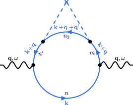
FIG. 4: Polarization bubble with two disorder (dashed) lines, leading to e-e-impurity skew scattering. Inner labels indicate the band indices, energy arguments of the Green functions are omitted. The upper half of the bubble corresponds to the leading disorder-induced off-diagonal correction to the Green functions, $G_{V,n^{\prime}m}^{R,A,K}(\boldsymbol{k}+\boldsymbol{q},\epsilon+\omega)$ [Eqs. (80), (81)]. There is an additional diagram with the disorder lines connected to the lower half of the bubble.

$$\left[\Pi^{R}(\boldsymbol{q},\omega)-\Pi^{A}(\boldsymbol{q},\omega)\right]_{\textrm{V}} =-\frac{1}{4}\gamma\sum_{n,n^{\prime},n_{2}}\sum_{m\neq n^{\prime}}\intop_{\boldsymbol{k},\boldsymbol{q}^{\prime}}\intop\frac{d\epsilon}{2\pi}\{Z_{n\boldsymbol{k}\rightarrow m,\boldsymbol{k}+\boldsymbol{q}\rightarrow n_{2},\boldsymbol{k}+\boldsymbol{q}+\boldsymbol{q}^{\prime}\rightarrow n^{\prime},\boldsymbol{k}+\boldsymbol{q}}$$

$$\times\left(F_{n_{2}}-F_{n^{\prime}}\right) \left(G_{0,n}^{R}-G_{0,n}^{A}\right)\left(G_{0,n^{\prime}}^{R}-G_{0,n^{\prime}}^{A}\right)\left(G_{0,n_{2}}^{R}-G_{0,n_{2}}^{A}\right)\left(G_{0,m}^{R}+G_{0,m}^{A}\right)-\left[\boldsymbol{q},\omega\rightarrow-\boldsymbol{q},-\omega\right]\},$$ (94)

$$\left[\Pi^{K}(\boldsymbol{q},\omega)\right]_{\textrm{V}} =\frac{1}{4}\gamma\sum_{n,n^{\prime},n_{2}}\sum_{m\neq n^{\prime}}\intop_{\boldsymbol{k},\boldsymbol{q}^{\prime}}\intop\frac{d\epsilon}{2\pi}\{Z_{n\boldsymbol{k}\rightarrow m,\boldsymbol{k}+\boldsymbol{q}\rightarrow n_{2},\boldsymbol{k}+\boldsymbol{q}+\boldsymbol{q}^{\prime}\rightarrow n^{\prime},\boldsymbol{k}+\boldsymbol{q}}$$

$$\times F_{n}\left(F_{n_{2}}-F_{n^{\prime}}\right) \left(G_{0,n}^{R}-G_{0,n}^{A}\right)\left(G_{0,n^{\prime}}^{R}-G_{0,n^{\prime}}^{A}\right)\left(G_{0,n_{2}}^{R}-G_{0,n_{2}}^{A}\right)\left(G_{0,m}^{R}+G_{m}^{A}\right)+\left[\boldsymbol{q},\omega\rightarrow-\boldsymbol{q},-\omega\right]\},$$ (95)

with $Z_{n_{1}\boldsymbol{k}_{1}\rightarrow n_{2}\boldsymbol{k}_{2}\rightarrow n_{3}\boldsymbol{k}_{3}\rightarrow n_{4}\boldsymbol{k}_{4}}$ being the imaginary part of the Bloch phase acquired during hopping,

$$Z_{n_{1}\boldsymbol{k}_{1}\rightarrow n_{2}\boldsymbol{k}_{2}\rightarrow n_{3}\boldsymbol{k}_{3}\rightarrow n_{4}\boldsymbol{k}_{4}}\equiv\textrm{Im}\left[\left\langle u_{n_{1}\boldsymbol{k}_{1}}|u_{n_{2}\boldsymbol{k}_{2}}\right\rangle\left\langle u_{n_{2}\boldsymbol{k}_{2}}|u_{n_{3}\boldsymbol{k}_{3}}\right\rangle\left\langle u_{n_{3}\boldsymbol{k}_{3}}|u_{n_{4}\boldsymbol{k}_{4}}\right\rangle\left\langle u_{n_{4}\boldsymbol{k}_{4}}|u_{n_{1}\boldsymbol{k}_{1}}\right\rangle\right].$$ (96)

For brevity, we have omitted the momentum and energy dependences of the Green functions, which can be read from the associated momentum to the Bloch wavefunctions, e.g., $G_{0,n^{\prime}}^{R}=G_{0,n^{\prime}}^{R}(\boldsymbol{k}+\boldsymbol{q},\epsilon+\omega)$ (functions related to the state $n,\boldsymbol{k}$ are evaluated on energy $\epsilon$ and all the rest are evaluated at energy $\epsilon+\omega$, since the disorder scattering does not transfer energy).

In the 2-band model, we can simplify the Bloch phase appearing in Eqs. (94), (95) and write (utilizing $m\neq n^{\prime})$

$$Z_{n\boldsymbol{k}\rightarrow m,\boldsymbol{k}+\boldsymbol{q}\rightarrow n_{2},\boldsymbol{k}+\boldsymbol{q}+\boldsymbol{q}^{\prime}\rightarrow n^{\prime},\boldsymbol{k}+\boldsymbol{q}} =-\textrm{Im}\left[\left\langle u_{n\boldsymbol{k}}|u_{n_{2},\boldsymbol{k}+\boldsymbol{q}+\boldsymbol{q}^{\prime}}\right\rangle\left\langle u_{n_{2},\boldsymbol{k}+\boldsymbol{q}+\boldsymbol{q}^{\prime}}|u_{n^{\prime},\boldsymbol{k}+\boldsymbol{q}}\right\rangle\left\langle u_{n^{\prime},\boldsymbol{k}+\boldsymbol{q}}|u_{n\boldsymbol{k}}\right\rangle\right].$$

$$\equiv -Z_{n\boldsymbol{k}\rightarrow n_{2},\boldsymbol{k}+\boldsymbol{q}+\boldsymbol{q}^{\prime}\rightarrow n^{\prime},\boldsymbol{k}+\boldsymbol{q}},$$ (97)

The Bloch phase acquired from 3 hoppings is given by (measuring momentum relative to the Weyl node) [72]

$$Z_{n_{1}\boldsymbol{k}_{1}\rightarrow n_{2}\boldsymbol{k}_{2}\rightarrow n_{3}\boldsymbol{k}_{3}}=\frac{\xi}{4}n_{1}n_{2}n_{3}\left(\hat{\boldsymbol{k}}_{1}\times\hat{\boldsymbol{k}}_{2}\right)\cdot\hat{\boldsymbol{k}}_{3},$$ (98)

where we remind that we are treating each node with chirality $\xi$ separately, assuming no internode scattering. We note that for a more general node Hamiltonian of the form $H_{\xi}=\xi\boldsymbol{h}(\boldsymbol{k})\cdot\boldsymbol{\sigma}$, one should replace $\hat{\boldsymbol{k}}\rightarrow\hat{\boldsymbol{h}}$ in Eq. (98). Substituting the corrections $\Pi_{\textrm{V}}^{R,A,K}$ [Eqs. (94), (95)] into the interlayer collision integral [Eq. (54)], we find the e-e-impurity skew-scattering part of the collision integral (summing over the two Weyl nodes)

$$I_{\boldsymbol{k}}^{\textrm{e-e-imp (p,a)}} =-W\sum_{\xi=\pm 1}\sum_{nn^{\prime}}\intop_{\boldsymbol{q},\boldsymbol{k}_{1},\boldsymbol{k}_{1^{\prime}}}$$

$$\times \left[f_{\boldsymbol{k}}^{\textrm{p}}f_{n\boldsymbol{k}_{1}}^{\textrm{a}}\left(1-f_{\boldsymbol{k}+\boldsymbol{q}}^{\textrm{p}}\right)\left(1-f_{n^{\prime}\boldsymbol{k}_{1^{\prime}}}^{\textrm{a}}\right)w_{\boldsymbol{k},n\boldsymbol{k}_{1}\rightarrow\boldsymbol{k}+\boldsymbol{q},n^{\prime}\boldsymbol{k}_{1^{\prime}}}^{\textrm{e-e-imp}}-\left(\boldsymbol{k},n\boldsymbol{k}_{1}\leftrightarrow\boldsymbol{k}+\boldsymbol{q},n^{\prime}\boldsymbol{k}_{1^{\prime}}\right)\right],$$ (99)

with

$$w_{\boldsymbol{k},n\boldsymbol{k}_{1}\rightarrow\boldsymbol{k}+\boldsymbol{q},n^{\prime}\boldsymbol{k}_{1^{\prime}}}^{\textrm{e-e-imp}} \equiv 4\pi^{2}\gamma\left|U_{RPA}^{R}(\boldsymbol{q},\omega)\right|^{2}\delta\left(\epsilon_{n\boldsymbol{k}_{1}}^{\textrm{a}}+\epsilon_{\boldsymbol{k}}^{\textrm{p}}-\epsilon_{n^{\prime}\boldsymbol{k}_{1^{\prime}}}^{\textrm{a}}-\epsilon_{\boldsymbol{k}+\boldsymbol{q}}^{\textrm{p}}\right)$$

$$\times\sum_{n_{2}}\intop_{\boldsymbol{k}_{2}}\left\{\frac{Z_{n\boldsymbol{k}_{1}\rightarrow n^{\prime}\boldsymbol{k}_{1^{\prime}}\rightarrow n_{2}\boldsymbol{k}_{2}}}{\epsilon_{n\boldsymbol{k}_{1}}^{\textrm{a}}-\epsilon_{\bar{n}\boldsymbol{k}_{1}}^{\textrm{a}}}\delta\left(\epsilon_{n\boldsymbol{k}_{1}}^{\textrm{a}}-\epsilon_{n_{2}\boldsymbol{k}_{2}}^{\textrm{a}}\right)\delta_{\boldsymbol{k}_{1}-\boldsymbol{q}-\boldsymbol{k}_{1^{\prime}}}-\left[n\boldsymbol{k}_{1}\leftrightarrow n_{2}\boldsymbol{k}_{2}\right]\right\}$$

$$+\left[\boldsymbol{k},n\boldsymbol{k}_{1}\leftrightarrow\boldsymbol{k}+\boldsymbol{q},n^{\prime}\boldsymbol{k}_{1^{\prime}}\right],$$ (100)

where $\bar{n}\equiv-n$. Note that $w^{\textrm{e-e-imp}}$ includes parts where the total electron momentum is not conserved, but is rather gained or lost due to the impurity scattering. In the level of a linearized collision integral, some simplifications can be made due to the anti-symmetry in $[n\boldsymbol{k}_{1}\leftrightarrow n_{2}\boldsymbol{k}_{2}]$ and $[n^{\prime}\boldsymbol{k}_{1^{\prime}}\leftrightarrow n_{2}\boldsymbol{k}_{2}]$ in Eq. (100). We find the linearized collision integral

$${\cal I}_{\boldsymbol{k}}^{\textrm{e-e-imp (p,a)}} =-W\sum_{\xi=\pm 1}\intop_{\boldsymbol{k}^{\prime},\boldsymbol{k}_{1},\boldsymbol{k}_{1^{\prime}}}f_{0}(\epsilon_{\boldsymbol{k}}^{\textrm{p}})f_{0}(\epsilon_{n\boldsymbol{k}_{1}}^{\textrm{a}})\left(1-f_{0}(\epsilon_{\boldsymbol{k}^{\prime}}^{\textrm{p}})\right)\left(1-f_{0}(\epsilon_{n^{\prime}\boldsymbol{k}_{1^{\prime}}}^{\textrm{a}})\right)$$

$$\times \left[g_{n\boldsymbol{k}_{1}}^{\textrm{a}}{\cal W}_{\boldsymbol{k},n\boldsymbol{k}_{1}\rightarrow\boldsymbol{k}^{\prime},n^{\prime}\boldsymbol{k}_{1^{\prime}}}-g_{n^{\prime}\boldsymbol{k}_{1^{\prime}}}^{\textrm{a}}{\cal W}_{\boldsymbol{k}^{\prime},n^{\prime}\boldsymbol{k}_{1^{\prime}}\rightarrow\boldsymbol{k},n\boldsymbol{k}_{1}}\right],$$ (101)

with

$${\cal W}_{\boldsymbol{k},n\boldsymbol{k}_{1}\rightarrow\boldsymbol{k}+\boldsymbol{q},n^{\prime}\boldsymbol{k}_{1^{\prime}}} ={\cal W}_{\boldsymbol{k},n\boldsymbol{k}_{1}\rightarrow\boldsymbol{k}+\boldsymbol{q},n^{\prime}\boldsymbol{k}_{1^{\prime}}}^{(1)}+{\cal W}_{\boldsymbol{k},n\boldsymbol{k}_{1}\rightarrow\boldsymbol{k}+\boldsymbol{q},n^{\prime}\boldsymbol{k}_{1^{\prime}}}^{(2)},$$ (102)

$${\cal W}_{\boldsymbol{k},n\boldsymbol{k}_{1}\rightarrow\boldsymbol{k}+\boldsymbol{q},n^{\prime}\boldsymbol{k}_{1^{\prime}}}^{(1)} =\frac{\pi^{2}\gamma}{2}\left|U_{\textrm{RPA}}^{R}(\boldsymbol{q},\omega)\right|^{2}\delta(\epsilon_{\boldsymbol{k}}^{\textrm{p}}+\epsilon_{n\boldsymbol{k}_{1}}^{\textrm{a}}-\epsilon_{\boldsymbol{k}+\boldsymbol{q}}^{\textrm{p}}-\epsilon_{n^{\prime}\boldsymbol{k}_{1^{\prime}}}^{\textrm{a}})\delta_{\boldsymbol{k}_{1}-\boldsymbol{k}_{1}^{\prime}-\boldsymbol{q}}\frac{\nu(\epsilon_{n\boldsymbol{k}_{1}}^{\textrm{a }})}{\epsilon_{n\boldsymbol{k}_{1}}^{\textrm{a }}}\left(\hat{\boldsymbol{k}}_{1}\times\hat{\boldsymbol{k}}_{1^{\prime}}\right)\cdot\boldsymbol{M}(\epsilon_{n\boldsymbol{k}_{1}}^{\textrm{a }}),$$ (103)

$${\cal W}_{\boldsymbol{k},n\boldsymbol{k}_{1}\rightarrow\boldsymbol{k}+\boldsymbol{q},n^{\prime}\boldsymbol{k}_{1^{\prime}}}^{(2)} =\frac{\pi^{2}\gamma}{2}\left|U_{\textrm{RPA}}^{R}(\boldsymbol{q},\omega)\right|^{2}\delta(\epsilon_{\boldsymbol{k}}^{\textrm{p}}+\epsilon_{n\boldsymbol{k}_{1}}^{\textrm{a}}-\epsilon_{\boldsymbol{k}+\boldsymbol{q}}^{\textrm{p}}-\epsilon_{n^{\prime}\boldsymbol{k}_{1^{\prime}}}^{\textrm{a}})\delta(\epsilon_{n_{2}\boldsymbol{k}}^{\textrm{a}}-\epsilon_{n\boldsymbol{k}_{1}}^{\textrm{a }})\frac{q\xi}{v_{F}\left(k_{1^{\prime}}\right)^{2}}\left(\hat{\boldsymbol{k}}_{1}\times\hat{\boldsymbol{k}}_{1^{\prime}}\right)\cdot\hat{\boldsymbol{q}},$$ (104)

where we assumed $k_{1^{\prime}},k_{1}\gg q$ (as is the case for Coulomb drag in the regime $k_{F}\gg 1/d$) and defined the average spinor on the Fermi surface of a single node

$$\boldsymbol{M}(\epsilon)\equiv\frac{1}{\nu(\epsilon)}\sum_{n}\intop_{\boldsymbol{k}}\delta\left(\epsilon_{n\boldsymbol{k}}^{\textrm{a}}-\epsilon\right)n\xi\hat{\boldsymbol{k}}.$$ (105)

Let us comment on a peculiarity regarding the symmetry of the e-e-impurity scattering rate under the exchange of incoming and outgoing particles, $\boldsymbol{k},n\boldsymbol{k}_{1}\leftrightarrow\boldsymbol{k}^{\prime},n^{\prime}\boldsymbol{k}_{1^{\prime}}$. The full rate $w^{\textrm{e-e-imp}}$ is symmetric under the exchange, as is explicitly seen from the exchanged term in Eq. (100). However, in the linearized response level, the term ${\cal W}_{\boldsymbol{k},n\boldsymbol{k}_{1}\rightarrow\boldsymbol{k}^{\prime},n^{\prime}\boldsymbol{k}_{1^{\prime}}}$ [Eq. (102)] contains a significant anti-symmetric part. This apparent contradiction is resolved by the fact that $w^{\textrm{e-e-imp}}$ contains non-momentum conserving terms [e.g., the second term in the curly brackets in Eq. (100) where $n\boldsymbol{k}_{1}\leftrightarrow n_{2}\boldsymbol{k}_{2}$, exchanging between the incoming and intermediate electrons]. In the linearized collision integral [Eq. (101)], we dropped terms that cancel under the integration over the angle of the outgoing electron, e.g., under $\intop_{\boldsymbol{k}_{1^{\prime}}}\delta(\epsilon_{\boldsymbol{k}_{1^{\prime}}}-\epsilon)g_{\boldsymbol{k}_{1}}w_{\boldsymbol{k},n\boldsymbol{k}_{1}\rightarrow\boldsymbol{k}+\boldsymbol{q},n^{\prime}\boldsymbol{k}_{1^{\prime}}}^{\textrm{e-e-imp}}$ for a fixed $\epsilon$. For a typical momentum-conserving integral, such integration only picks the momentum delta function and cannot alter the symmetry of $w$. However, in our case, this integration cancels a pair of terms anti-symmetric in $n^{\prime}\boldsymbol{k}_{1^{\prime}}\leftrightarrow n_{2}\boldsymbol{k}_{2}$, resulting in a non-symmetric scattering rate ${\cal W}_{\boldsymbol{k},n\boldsymbol{k}_{1}\rightarrow\boldsymbol{k}+\boldsymbol{q},n^{\prime}\boldsymbol{k}_{1^{\prime}}}$.

Appendix B Drag force from the e-e collision integral

Here, we compute the drag force (momentum transfer rate) between the layers for boosted distribution functions [Eqs. (26), (27) and (38) of the main text] and an interlayer scattering integral given by Eq. (20) with the scattering rates of Eq. (25). We show that the drag force can be written in the form of Eqs. (30), (40) in the main text, and calculate explicitly the drag coefficients $\eta_{\parallel,H}^{D}$. We separate the calculation for each term in the scattering rate.

B.1 Born-approximation part of the scattering rate

The Born-approximation part of $w^{\textrm{e-e}}$ is symmetric and conserves momentum, $w_{\boldsymbol{k},n\boldsymbol{k}_{1}+\boldsymbol{q}\rightarrow\boldsymbol{k}+\boldsymbol{q},n^{\prime}\boldsymbol{k}_{1}}^{\textrm{Born}}=w_{\boldsymbol{k}+\boldsymbol{q},n^{\prime}\boldsymbol{k}_{1}\rightarrow\boldsymbol{k},n\boldsymbol{k}_{1}+\boldsymbol{q}}^{\textrm{Born}}$. We substitute $w^{\textrm{e-e}}\rightarrow w^{\textrm{Born}}$ in Eq. (20), linearize the collision integral with respect to the non-equilibrium part of the distribution functions, utilize the energy and momentum conservation of the collision integral, and arrive at

$${\cal I}_{\boldsymbol{k}}^{\textrm{Born (p,a)}}\left[f^{\textrm{p}},f^{\textrm{a}}\right] =-\frac{W}{4}\sum_{\xi=\pm 1}\sum_{nn^{\prime}}\intop_{\boldsymbol{q},\boldsymbol{k}_{1}}\frac{w_{\boldsymbol{k},n\boldsymbol{k}_{1}+\boldsymbol{q}\rightarrow\boldsymbol{k}+\boldsymbol{q},n^{\prime}\boldsymbol{k}_{1}}^{\textrm{Born}}}{\sinh^{2}\frac{\omega}{2T}}\left(f_{0}(\epsilon_{\boldsymbol{k}+\boldsymbol{q}}^{\textrm{p}})-f_{0}(\epsilon_{\boldsymbol{k}}^{\textrm{p}})\right)\left(f_{0}(\epsilon_{n\boldsymbol{k}_{1}+\boldsymbol{q}}^{\textrm{a}})-f_{0}(\epsilon_{n^{\prime}\boldsymbol{k}_{1}}^{\textrm{a}})\right)$$

$$\times \left(g_{\boldsymbol{k}}^{\textrm{p}}+g_{n\boldsymbol{k}_{1}+\boldsymbol{q}}^{\textrm{a}}-g_{\boldsymbol{k}+\boldsymbol{q}}^{\textrm{p}}-g_{n^{\prime}\boldsymbol{k}_{1}}^{\textrm{a}}\right),$$ (106)

where $\omega\equiv\epsilon_{\boldsymbol{k}+\boldsymbol{q}}^{\textrm{p}}-\epsilon_{\boldsymbol{k}}^{\textrm{p}}=\epsilon_{n\boldsymbol{k}_{1}+\boldsymbol{q}}^{\textrm{a}}-\epsilon_{n^{\prime}\boldsymbol{k}_{1}}^{\textrm{a}}$. The drag force between the layers is obtained by multiplying Eq. (106) by $\boldsymbol{k}$ and integrating over $\boldsymbol{k}$,

$$\boldsymbol{F}^{\textrm{p,a (Born)}} \equiv\intop_{\boldsymbol{k}}\boldsymbol{k}{\cal I}_{\boldsymbol{k}}^{\textrm{Born (p,a)}}=-\frac{W}{4}\sum_{\xi=\pm 1}\sum_{nn^{\prime}}\intop_{\boldsymbol{k},\boldsymbol{q},\boldsymbol{k}_{1}}\boldsymbol{k}\frac{w_{\boldsymbol{k},n\boldsymbol{k}_{1}+\boldsymbol{q}\rightarrow\boldsymbol{k}+\boldsymbol{q},n^{\prime}\boldsymbol{k}_{1}}^{\textrm{Born}}}{\sinh^{2}\frac{\omega}{2T}}$$

$$\times\left(f_{0}(\epsilon_{\boldsymbol{k}+\boldsymbol{q}}^{\textrm{p}})-f_{0}(\epsilon_{\boldsymbol{k}}^{\textrm{p}})\right)\left(f_{0}(\epsilon_{n\boldsymbol{k}_{1}+\boldsymbol{q}}^{\textrm{a}})-f_{0}(\epsilon_{n^{\prime}\boldsymbol{k}_{1}}^{\textrm{a}})\right)\left(g_{\boldsymbol{k}}^{\textrm{p}}+g_{n\boldsymbol{k}_{1}+\boldsymbol{q}}^{\textrm{a}}-g_{\boldsymbol{k}+\boldsymbol{q}}^{\textrm{p}}-g_{n^{\prime}\boldsymbol{k}_{1}}^{\textrm{a}}\right).$$ (107)

The expression above may be simplified by adding the opposite scattering process to the integrand. Concretely, writing the integral as $\intop_{\boldsymbol{q},\boldsymbol{k},\boldsymbol{k}^{\prime}}h(\boldsymbol{k},\boldsymbol{k}^{\prime},\boldsymbol{q})$, we rename the integration variables $\boldsymbol{k},\boldsymbol{k}^{\prime},\boldsymbol{q}\rightarrow\boldsymbol{k}+\boldsymbol{q},\boldsymbol{k}^{\prime}+\boldsymbol{q},-\boldsymbol{q}$ and rewrite the integral as $\intop_{\boldsymbol{q},\boldsymbol{k},\boldsymbol{k}^{\prime}}h(\boldsymbol{k},\boldsymbol{k}^{\prime},\boldsymbol{q})=\frac{1}{2}\intop_{\boldsymbol{q},\boldsymbol{k},\boldsymbol{k}^{\prime}}\left(h(\boldsymbol{k},\boldsymbol{k}^{\prime},\boldsymbol{q})+h(\boldsymbol{k}+\boldsymbol{q},\boldsymbol{k}^{\prime}+\boldsymbol{q},-\boldsymbol{q})\right)$. Doing this for the integral in Eq. (107) leads to

$$\boldsymbol{F}^{\textrm{p,a (Born)}} =\frac{W}{8T}\sum_{\xi=\pm 1}\sum_{nn^{\prime}}\intop_{\boldsymbol{q},\boldsymbol{k},\boldsymbol{k}_{1}}\boldsymbol{q}\frac{w_{\boldsymbol{k},n\boldsymbol{k}_{1}+\boldsymbol{q}\rightarrow\boldsymbol{k}+\boldsymbol{q},n^{\prime}\boldsymbol{k}_{1}}^{\textrm{Born}}}{\sinh^{2}\frac{\omega}{2T}}\left(f_{0}(\epsilon_{\boldsymbol{k}+\boldsymbol{q}}^{\textrm{p}})-f_{0}(\epsilon_{\boldsymbol{k}}^{\textrm{p}})\right)\left(f_{0}(\epsilon_{n\boldsymbol{k}_{1}+\boldsymbol{q}}^{\textrm{a}})-f_{0}(\epsilon_{n^{\prime}\boldsymbol{k}_{1}}^{\textrm{a}})\right)$$

$$\times\left[g_{\boldsymbol{k}}^{\textrm{p}}+g_{n\boldsymbol{k}_{1}+\boldsymbol{q}}^{\textrm{a}}-g_{\boldsymbol{k}+\boldsymbol{q}}^{\textrm{p}}-g_{n^{\prime}\boldsymbol{k}_{1}}^{\textrm{a}}\right].$$ (108)

We now use Eq. (108) to calculate the drag force for the case where the distribution functions are boosted velocity distributions, and treat the more general case of energy-dependent boost velocities later.

Simple case: boosted velocity distributions

For boosted velocity distributions, $g_{n\boldsymbol{k}}^{l}=\boldsymbol{k}\cdot\boldsymbol{u}^{l}/T$. Substituting into Eq. (108) leads to

$$\boldsymbol{F}^{\textrm{p,a (Born)}} =\frac{W}{8T}\sum_{\xi=\pm 1}\sum_{nn^{\prime}}\intop_{\boldsymbol{q},\boldsymbol{k},\boldsymbol{k}_{1}}\boldsymbol{q}\left[\boldsymbol{q}\cdot\left(\boldsymbol{u}^{\textrm{a}}-\boldsymbol{u}^{\textrm{p}}\right)\right]$$

$$\times\frac{w_{\boldsymbol{k},n\boldsymbol{k}_{1}+\boldsymbol{q}\rightarrow\boldsymbol{k}+\boldsymbol{q},n^{\prime}\boldsymbol{k}_{1}}^{\textrm{Born}}}{\sinh^{2}\frac{\omega}{2T}}\left(f_{0}(\epsilon_{\boldsymbol{k}+\boldsymbol{q}}^{\textrm{p}})-f_{0}(\epsilon_{\boldsymbol{k}}^{\textrm{p}})\right)\left(f_{0}(\epsilon_{n\boldsymbol{k}_{1}+\boldsymbol{q}}^{\textrm{a}})-f_{0}(\epsilon_{n^{\prime}\boldsymbol{k}_{1}}^{\textrm{a}})\right).$$ (109)

For any isotropic system, this results in the drag force

$$\boldsymbol{F}^{\textrm{p,a (Born)}}=\frac{\eta_{\parallel}^{D}}{d}\left(\boldsymbol{u}^{\textrm{a}}-\boldsymbol{u}^{\textrm{p}}\right),$$ (110)

with the drag coefficient $\eta_{\parallel}^{D}$ given by

$$\eta_{\parallel}^{D}=\frac{Wd}{16T}\sum_{\xi=\pm 1}\sum_{nn^{\prime}}\intop_{\boldsymbol{q},\boldsymbol{k},\boldsymbol{k}_{1}}\frac{q^{2}}{\sinh^{2}\frac{\omega}{2T}}w_{\boldsymbol{k},n\boldsymbol{k}_{1}+\boldsymbol{q}\rightarrow\boldsymbol{k}+\boldsymbol{q},n^{\prime}\boldsymbol{k}_{1}}^{\textrm{Born}}\left(f_{0}(\epsilon_{\boldsymbol{k}+\boldsymbol{q}}^{\textrm{p}})-f_{0}(\epsilon_{\boldsymbol{k}}^{\textrm{p}})\right)\left(f_{0}(\epsilon_{n\boldsymbol{k}_{1}+\boldsymbol{q}}^{\textrm{a}})-f_{0}(\epsilon_{n^{\prime}\boldsymbol{k}_{1}}^{\textrm{a}})\right).$$ (111)

Substituting the specific form of $w^{\textrm{Born}}$, Eq. (84), we obtain

$$\eta_{\parallel}^{D}=\frac{Wd}{8\pi T}\intop_{-\infty}^{\infty}d\omega\frac{1}{\sinh^{2}\frac{\omega}{2T}}\intop_{\boldsymbol{q}}q^{2}\left|U_{\textrm{RPA}}^{R}(\boldsymbol{q},\omega)\right|^{2}\textrm{Im}\Pi_{0}^{\textrm{p,}R}(\boldsymbol{q},\omega)\textrm{Im}\Pi_{0}^{\textrm{a,}R}(\boldsymbol{q},\omega),$$ (112)

where $\Pi_{0}^{l,R}(\boldsymbol{q},\omega)$ are the bare polarization operators of the layers, with their imaginary parts given by

$$\textrm{Im}\Pi_{0}^{\textrm{p,}R}(\boldsymbol{q},\omega) =\pi\intop_{\boldsymbol{k}}\delta(\epsilon_{\boldsymbol{k}+\boldsymbol{q}}^{\textrm{p}}-\epsilon_{\boldsymbol{k}}^{\textrm{p }}-\omega)\left(f_{0}(\epsilon_{\boldsymbol{k}+\boldsymbol{q}}^{\textrm{p}})-f_{0}(\epsilon_{\boldsymbol{k}}^{\textrm{p }})\right),$$ (113)

$$\textrm{Im}\Pi_{0}^{\textrm{a,}R}(\boldsymbol{q},\omega) =\pi\sum_{\xi=\pm 1}\sum_{nn^{\prime}}\intop_{\boldsymbol{k}}\delta(\epsilon_{n\boldsymbol{k}+\boldsymbol{q}}^{\textrm{a }}-\epsilon_{n^{\prime}\boldsymbol{k}}^{\textrm{a }}-\omega)\left(f_{0}(\epsilon_{n\boldsymbol{k}+\boldsymbol{q}}^{\textrm{a }})-f_{0}(\epsilon_{n^{\prime}\boldsymbol{k}}^{\textrm{a }})\right)\left|\left\langle u_{n^{\prime}\boldsymbol{k}}|u_{n\boldsymbol{k}+\boldsymbol{q}}\right\rangle\right|^{2}.$$ (114)

Evaluating Eq. (112) with the approximate Coulomb interaction [Eq. (53)] in the limits $T\ll T_{d}$ and $T\gg T_{d}$ leads to Eqs. (31) and (41) of the main text. To briefly explain the calculation, in the limit $T\ll T_{d}$, the frequency integral in Eq. (112) is dominated by $\omega\sim T$ and the result breaks into the product of the independent $\omega$ and $\boldsymbol{q}$ integrals. In the limit $T\gg T_{d}$, the frequency integration is cut off by the boundary of the particle-hole spectrum in the layers, $\omega<\min(v_{F}^{\textrm{a}},v_{F}^{\textrm{p}})q$, and the $\omega$ and $\boldsymbol{q}$ integrals do not factorize [1]. The thermal factor can be approximated by $\sinh\left(\omega/2T\right)\approx\omega/\left(2T\right)$ [23]. Note that the frequency dependence of the interlayer scattering propagator $U_{\textrm{RPA}}^{R}(\boldsymbol{q},\omega)$ is important at high temperatures (see Sec. B.3 in this Appendix for more details about the calculation).

General case: energy-dependent boost velocities

We now consider the more general case, parametrizing the non-equilibrium distribution functions with an energy-dependent boost velocity $g_{n\boldsymbol{k}}^{\textrm{a}}=\boldsymbol{k}\cdot\boldsymbol{u}^{\textrm{a}}(\epsilon_{n\boldsymbol{k}}^{\textrm{a }})/T$, as in Sec. IV.2.2 of the main text. For simplicity, we take $\boldsymbol{u}^{\textrm{p}}=0$. Substituting this form of $g_{n\boldsymbol{k}}^{\textrm{a}}$ in Eq. (108) yields

$$\boldsymbol{F}^{\textrm{p,a (Born)}} =\frac{W}{8T}\sum_{\xi=\pm 1}\sum_{nn^{\prime}}\intop_{\boldsymbol{q},\boldsymbol{k},\boldsymbol{k}_{1}}\boldsymbol{q}\frac{w_{\boldsymbol{k},n\boldsymbol{k}_{1}+\boldsymbol{q}\rightarrow\boldsymbol{k}+\boldsymbol{q},n^{\prime}\boldsymbol{k}_{1}}^{\textrm{Born}}}{\sinh^{2}\frac{\omega}{2T}}\left(f_{0}(\epsilon_{\boldsymbol{k}+\boldsymbol{q}}^{\textrm{p}})-f_{0}(\epsilon_{\boldsymbol{k}}^{\textrm{p}})\right)\left(f_{0}(\epsilon_{n\boldsymbol{k}_{1}+\boldsymbol{q}}^{\textrm{a}})-f_{0}(\epsilon_{n^{\prime}\boldsymbol{k}_{1}}^{\textrm{a}})\right)$$

$$\times\left[\left(\boldsymbol{k}_{1}+\boldsymbol{q}\right)\cdot\boldsymbol{u}^{\textrm{a}}(\epsilon_{n^{\prime}\boldsymbol{k}_{1}}^{\textrm{a}}+\omega)-\boldsymbol{k}_{1}\cdot\boldsymbol{u}^{\textrm{a}}(\epsilon_{n^{\prime}\boldsymbol{k}_{1}}^{\textrm{a}})\right].$$ (115)

Performing a Taylor expansion for $\boldsymbol{u}^{\textrm{a}}(\epsilon)$ up to the first-derivative term, we find

$$\boldsymbol{F}^{\textrm{p,a (Born)}} =\frac{W}{8T}\sum_{\xi=\pm 1}\sum_{nn^{\prime}}\intop_{\boldsymbol{q},\boldsymbol{k}_{1}}\boldsymbol{q}\frac{w_{\boldsymbol{k},n\boldsymbol{k}_{1}+\boldsymbol{q}\rightarrow\boldsymbol{k}+\boldsymbol{q},n^{\prime}\boldsymbol{k}_{1}}^{\textrm{Born}}}{\sinh^{2}\frac{\omega}{2T}}\left(f_{0}(\epsilon_{\boldsymbol{k}+\boldsymbol{q}}^{\textrm{p}})-f_{0}(\epsilon_{\boldsymbol{k}}^{\textrm{p}})\right)\left(f_{0}(\epsilon_{n\boldsymbol{k}_{1}+\boldsymbol{q}}^{\textrm{a}})-f_{0}(\epsilon_{n^{\prime}\boldsymbol{k}_{1}}^{\textrm{a}})\right)$$

$$\left[\boldsymbol{q}\cdot\boldsymbol{u}^{\textrm{a}}(\epsilon_{n^{\prime}\boldsymbol{k}_{1}}^{\textrm{a}})+\boldsymbol{k}_{1}\cdot\omega\frac{\partial\boldsymbol{u}^{\textrm{a}}(\epsilon_{n^{\prime}\boldsymbol{k}_{1}}^{\textrm{a}})}{\partial\epsilon_{n^{\prime}\boldsymbol{k}_{1}}^{\textrm{a}}}\right]\equiv\boldsymbol{F}^{\textrm{p,a}}[\boldsymbol{u}^{\textrm{a}}]+\boldsymbol{F}^{\textrm{p,a}}[\partial\boldsymbol{u}^{\textrm{a}}/\partial\epsilon].$$ (116)

In the limit where $\epsilon_{F}^{\textrm{a}}\gg T,T_{d}$, one may substitute $\boldsymbol{u}^{\textrm{a}}(\epsilon_{\boldsymbol{k}^{\prime}}^{\textrm{a }})\approx\boldsymbol{u}^{\textrm{a}}(\epsilon_{F}^{\textrm{a}})$ in the first term, returning to the case of the last section. The second term in Eq. (116) arises from the energy dependence of the boost velocity. We write it as

$$F_{\alpha}^{\textrm{p,a}}[\partial\boldsymbol{u}^{a}/\partial\epsilon]\equiv\eta_{\parallel(1)}^{D}\frac{\epsilon_{F}^{\textrm{a}}}{d}\left.\frac{\partial u_{\alpha}^{\textrm{a}}}{\partial\epsilon}\right|_{\epsilon=\epsilon_{F}^{\textrm{a}}}.$$ (117)

This part of the force corresponds to the third term in Eq. (40) of the main text, with the drag coefficient

$$\eta_{\parallel(1)}^{D}=\frac{Wd}{8\pi T}\int d\omega\frac{1}{\sinh^{2}\frac{\omega}{2T}}\intop_{\boldsymbol{q}}q^{2}\left(\frac{\omega}{v_{F}^{\textrm{a}}q}\right)^{2}\left|U_{\textrm{RPA}}^{R}(\boldsymbol{q},\omega)\right|^{2}\textrm{Im}\Pi_{0}^{\textrm{p,}R}(\boldsymbol{q},\omega)\textrm{Im}\Pi_{0}^{\textrm{a,}R}(\boldsymbol{q},\omega).$$ (118)

For an e-e scattering where the WSM electron scatters from (momentum, energy) $\left(\boldsymbol{k},\epsilon_{n\boldsymbol{k}}^{\textrm{a}}\right)\rightarrow\left(\boldsymbol{k}+\boldsymbol{q},\epsilon_{n^{\prime}\boldsymbol{k}+\boldsymbol{q}}^{\textrm{a}}=\epsilon_{n\boldsymbol{k}}^{\textrm{a}}+\omega\right)$, the factor $\omega/v_{F}^{\textrm{a}}q$ is equal to the cosine of the angle between $\boldsymbol{v}_{n\boldsymbol{k}}^{\textrm{a}}$ and $\boldsymbol{q}$ (for $k\sim k_{F}\gg q\sim 1/d$). Thus, this factor approaches one for forward scattering (i.e., for $\boldsymbol{q}\parallel\boldsymbol{v}_{n\boldsymbol{k}}^{\textrm{a}}$) and zero for perpendicular scattering ($\boldsymbol{q}\perp\boldsymbol{v}_{n\boldsymbol{k}}^{\textrm{a}}$). For low temperatures ($T\ll T_{d}$), perpendicular scattering is dominant ($\omega/v_{F}^{\textrm{a}}q\sim Td/v_{F}^{\textrm{a}}\ll 1$), and the resulting contribution to the drag from $\eta_{\parallel(1)}^{D}$ is subleading in $\left(T/T_{d}\right)^{2}$ compared to the $\eta_{\parallel(0)}^{D}$ term [Eq. (109)]. In the opposite limit where $T\gg T_{d}$, the two terms are comparable. We evaluate the integral with the approximated Coulomb interaction [Eq. (53)] to obtain the value of $\eta_{\parallel(1)}^{D}$ presented in Eq. (42) of the main text. Note that in the case $v_{F}^{\textrm{a}}\gg v_{F}^{\textrm{p}}$, interlayer collisions with forward scattering in the WSM are not possible, and the coefficient $\eta_{\parallel(1)}^{D}$ becomes parametrically small, as can be seen from Eq. (42).

B.2 Skew scattering

Next, we calculate the drag force from the skew-scattering parts of the e-e collision integral, corresponding to the e-e-impurity interference and side-jump modified e-e collision integrals.

e-e-impurity scattering

The linearized form of the e-e-impurity part of the collision integral is given in Eq. (101). We calculate the contributions from the two terms in the scattering rate ${\cal W}={\cal W}^{(1)}+{\cal W}^{(2)}$ [Eq. (102)] separately, writing ${\cal I}_{\boldsymbol{k}}^{\textrm{e-e-imp (p,a)}}={\cal I}_{\boldsymbol{k}}^{\textrm{e-e-imp (1)}}+{\cal I}_{\boldsymbol{k}}^{\textrm{e-e-imp (2)}}$. The term ${\cal W}^{(1)}$ is antisymmetric in incoming and outgoing particles, and the corresponding term in the collision integral is given by

$${\cal I}_{\boldsymbol{k}}^{\textrm{e-e-imp (1)}} =-\frac{W}{4}\sum_{\xi=\pm 1}\sum_{nn^{\prime}}\intop_{\boldsymbol{q},\boldsymbol{k}_{1}}\frac{{\cal W}_{\boldsymbol{k},n\boldsymbol{k}_{1}+\boldsymbol{q}\rightarrow\boldsymbol{k}+\boldsymbol{q},n^{\prime}\boldsymbol{k}_{1}}^{(1)}}{\sinh^{2}\frac{\omega}{2T}}\left(f_{0}(\epsilon_{\boldsymbol{k}+\boldsymbol{q}}^{\textrm{p}})-f_{0}(\epsilon_{\boldsymbol{k}}^{\textrm{p}})\right)\left(f_{0}(\epsilon_{n\boldsymbol{k}_{1}+\boldsymbol{q}}^{\textrm{a}})-f_{0}(\epsilon_{n^{\prime}\boldsymbol{k}_{1}}^{\textrm{a}})\right)$$

$$\times\left(g_{n\boldsymbol{k}_{1}+\boldsymbol{q}}^{\textrm{a}}+g_{n^{\prime}\boldsymbol{k}_{1}}^{\textrm{a}}\right),$$ (119)

where we utilized the momentum conservation of ${\cal W}^{(1)}$ to eliminate one momentum integration. In the limit $k_{F}^{\textrm{a}}\gg 1/d$, the terms corresponding to $g_{n\boldsymbol{k}_{1}+\boldsymbol{q}}^{\textrm{a}}$ and $g_{n^{\prime}\boldsymbol{k}_{1}}^{\textrm{a}}$ in Eq. (119) give equal contributions, and we can simplify, substituting ${\cal W}^{(1)}$ from Eq. (103),

$${\cal I}_{\boldsymbol{k}}^{\textrm{e-e-imp (1)}} =-\frac{W}{8T}\intop_{-\infty}^{\infty}d\omega\frac{1}{\sinh^{2}\frac{\omega}{2T}}\intop_{\boldsymbol{q}}\left(f_{0}(\epsilon_{\boldsymbol{k}+\boldsymbol{q}}^{\textrm{p}})-f_{0}(\epsilon_{\boldsymbol{k}}^{\textrm{p}})\right)\delta(\epsilon_{\boldsymbol{k}+\boldsymbol{q}}^{\textrm{p}}-\epsilon_{\boldsymbol{k}}^{\textrm{p}}-\omega)$$

$$\times\left|U_{\textrm{RPA}}^{R}(\boldsymbol{q},\omega)\right|^{2}\left[1-\left(\frac{\omega}{v_{F}^{\textrm{a}}q}\right)^{2}\right]\textrm{Im}\Pi_{0}^{\textrm{a,}R}(\boldsymbol{q},\omega)\frac{C}{\epsilon_{F}^{\textrm{a}}\tau^{\textrm{a}}}\epsilon_{\alpha\beta}q_{\alpha}u_{\beta}^{\textrm{a}}.$$ (120)

Calculating the corresponding drag force in the same manner as in the previous subsection, we find

$$F_{\alpha}^{\textrm{e-e-imp (1)}} \equiv\intop_{\boldsymbol{k}}k_{\alpha}{\cal I}_{\boldsymbol{k}}^{\textrm{e-e-imp (1)}}$$

$$=-\frac{W}{32\pi T}\frac{C}{\epsilon_{F}^{\textrm{a}}\tau^{\textrm{a}}}\intop_{-\infty}^{\infty}d\omega\frac{1}{\sinh^{2}\frac{\omega}{2T}}\intop_{\boldsymbol{q}}q^{2}\left|U_{\textrm{RPA}}^{R}(\boldsymbol{q},\omega)\right|^{2}\left[1-\left(\frac{\omega}{v_{F}^{\textrm{a}}q}\right)^{2}\right]\textrm{Im}\Pi_{0}^{\textrm{p,}R}(\boldsymbol{q},\omega)\textrm{Im}\Pi_{0}^{\textrm{a,}R}(\boldsymbol{q},\omega)\epsilon_{\alpha\beta}u_{\beta}^{\textrm{a}}.$$ (121)

This corresponds to a Hall-like drag force, $F_{\alpha}^{\textrm{e-e-imp (1)}}\sim\epsilon_{\alpha\beta}\eta_{H(\textrm{e-e-imp,1)}}^{D}u_{\beta}^{\textrm{a}}/d$ [second term in Eq. (30)], with

$$\eta_{H(\textrm{e-e-imp,1)}}^{D}=-\frac{C}{4\epsilon_{F}^{\textrm{a}}\tau^{\textrm{a}}}\eta_{D}^{\parallel}Q_{3}(\frac{v_{F}^{\textrm{p}}}{v_{F}^{\textrm{a}}}),$$ (122)

and $Q_{3}(z)$ given in Eq. (132). The calculation for the contribution from ${\cal I}_{\boldsymbol{k}}^{\textrm{e-e-imp (2)}}$ is similar, and leads to $\eta_{H(\textrm{e-e-imp,2)}}^{D}=\eta_{H(\textrm{e-e-imp,1)}}^{D}/3$. In total, e-e-impurity scattering generates the drag force $F_{\alpha}^{\textrm{{p,a ({e-e-imp)}}}}=\eta_{H(\textrm{e-e-imp)}}^{D}\epsilon_{\alpha\beta}u_{\beta}^{\textrm{a}}/d$, with

$$\eta_{H(\textrm{e-e-imp)}}^{D}=\frac{4}{3}\eta_{H(\textrm{e-e-imp,1)}}^{D}.$$ (123)

Side-jump collision integral

Next, we calculate the contribution from the side-jump correction to the e-e collision integral, Eq. (92). Since the electric field is explicit in the scattering rate, in the linear response level we substitute the equilibrium value of the distribution functions, obtaining

$${\cal I}_{\boldsymbol{k}}^{\textrm{s.j. (p,a)}} =\frac{\pi W}{2T}\sum_{\xi=\pm 1}\sum_{nn^{\prime}}\intop_{\boldsymbol{k}_{1},\boldsymbol{q}}\frac{1}{\sinh^{2}(\frac{\omega}{2T})}\left|U_{\textrm{RPA}}^{R}(\boldsymbol{q},\omega)\right|^{2}\delta(\epsilon_{\boldsymbol{k}}^{\textrm{p}}+\epsilon_{n\boldsymbol{k}_{1}+\boldsymbol{q}}^{\textrm{a}}-\epsilon_{\boldsymbol{k}+\boldsymbol{q}}^{\textrm{p}}-\epsilon_{n^{\prime}\boldsymbol{k}_{1}}^{\textrm{a}})$$

$$\times\left(f_{0}(\epsilon_{\boldsymbol{k}+\boldsymbol{q}}^{\textrm{p}})-f_{0}(\epsilon_{\boldsymbol{k}}^{\textrm{p}})\right)\left(f_{0}(\epsilon_{n\boldsymbol{k}_{1}+\boldsymbol{q}}^{\textrm{a}})-f_{0}(\epsilon_{n^{\prime}\boldsymbol{k}_{1}}^{\textrm{a}})\right)\left|\left\langle n\boldsymbol{k}_{1}+\boldsymbol{q}|n^{\prime}\boldsymbol{k}_{1}\right\rangle\right|^{2}\delta\boldsymbol{r}_{n\boldsymbol{k}_{1}+\boldsymbol{q},n^{\prime}\boldsymbol{k}_{1},}\cdot e\boldsymbol{E}.$$ (124)

Substituting the value of the coordinate shift for the Weyl electrons in a node of chirality $\xi$ [72]

$$\delta\boldsymbol{r}_{n\boldsymbol{k},n^{\prime}\boldsymbol{k}^{\prime}}=\xi\frac{\hat{\boldsymbol{k}}\times\hat{\boldsymbol{k}}^{\prime}}{4\left|\left\langle\boldsymbol{k}|\boldsymbol{k}^{\prime}\right\rangle\right|^{2}}\left(\frac{n^{\prime}}{k}+\frac{n}{k^{\prime}}\right),$$ (125)

we get

$${\cal I}_{\boldsymbol{k}}^{\textrm{s.j. (p,a)}} =-\frac{WC}{8T}\intop d\omega\frac{1}{4\sinh^{2}\frac{\omega}{2T}}\intop_{\boldsymbol{q}}\left|U_{\textrm{RPA}}^{R}(\boldsymbol{q},\omega)\right|^{2}\left(f_{0}(\epsilon_{\boldsymbol{k}+\boldsymbol{q}}^{\textrm{p}})-f_{0}(\epsilon_{\boldsymbol{k}}^{\textrm{p}})\right)\delta(\epsilon_{\boldsymbol{k}+\boldsymbol{q}}^{\textrm{p}}-\epsilon_{\boldsymbol{k}}^{\textrm{p}}-\omega)$$

$$\times\textrm{Im}\Pi_{0}^{\textrm{a,}R}(\boldsymbol{q},\omega)\left[1-\left(\frac{\omega}{v_{F}^{\textrm{a}}q}\right)^{2}\right]\left(\frac{v_{F}^{\textrm{a}}}{\epsilon_{F}^{\textrm{a}}}\right)^{2}\epsilon_{\alpha\beta}q_{\alpha}eE_{\beta}.$$ (126)

The resulting drag force is given by

$$F_{\alpha}^{\textrm{p,a (s.j.)}} =\intop_{\boldsymbol{k}}k_{\alpha}{\cal I}_{\boldsymbol{k}}^{\textrm{s.j. (p,a)}}$$

$$=-\frac{WC}{32\pi T}\intop d\omega\frac{1}{\sinh^{2}\frac{\omega}{2T}}\intop_{\boldsymbol{q}}\left|U_{\textrm{RPA}}^{R}(\boldsymbol{q},\omega)\right|^{2}\left[1-\left(\frac{\omega}{v_{F}^{\textrm{a}}q}\right)^{2}\right]\textrm{Im}\Pi_{0}^{\textrm{p,}R}(\boldsymbol{q},\omega)\textrm{Im}\Pi_{0}^{\textrm{a,}R}(\boldsymbol{q},\omega)$$

$$\times\left(\frac{v_{F}^{\textrm{a}}}{\epsilon_{F}^{\textrm{a}}}\right)^{2}q^{2}\epsilon_{\alpha\beta}eE_{\beta}.$$ (127)

The resulting force is perpendicular to the electric field in the active layer. Since $\boldsymbol{F}^{\textrm{p,a (s.j.)}}$ is already subleading in $\left(1/\epsilon_{F}^{\textrm{a}}\tau^{\textrm{a}}\right)$ compared to the leading part of $\boldsymbol{F}^{\textrm{p,a}}$, we can approximate $e\boldsymbol{E}^{\textrm{a}}\simeq\boldsymbol{u}^{\textrm{a}}\epsilon_{F}^{\textrm{a}}/\left(\left(v_{F}^{\textrm{a}}\right)^{2}\tau^{\textrm{a},\parallel}\right)=2\boldsymbol{u}^{\textrm{a}}\epsilon_{F}^{\textrm{a}}/\left(3\left(v_{F}^{\textrm{a}}\right)^{2}\tau^{\textrm{a}}\right)$ and write Eq. (127) as

$$F_{\alpha}^{\textrm{p,a (s.j.)}} =-\frac{WC}{48\pi T}\intop d\omega\frac{1}{\sinh^{2}\frac{\omega}{2T}}\intop_{\boldsymbol{q}}\left|U_{\textrm{RPA}}^{R}(\boldsymbol{q},\omega)\right|^{2}\left[1-\left(\frac{\omega}{v_{F}^{\textrm{a}}q}\right)^{2}\right]\textrm{Im}\Pi_{0}^{\textrm{p,}R}(\boldsymbol{q},\omega)\textrm{Im}\Pi_{0}^{\textrm{a,}R}(\boldsymbol{q},\omega)$$

$$\times\frac{1}{\epsilon_{F}^{\textrm{a}}\tau^{\textrm{a}}}q^{2}\epsilon_{\alpha\beta}u_{\beta}^{\textrm{a}}\equiv\eta_{H\textrm{(s.j.)}}^{D}\epsilon_{\alpha\beta}u_{\beta}^{\textrm{a}}/d,$$ (128)

with $\eta_{H\textrm{(s.j.)}}^{D}=\eta_{H\textrm{(e-e-imp)}}^{D}/2$. Summing the contributions from the e-e-impurity scattering and e-e-side-jump scattering, $F_{\alpha}^{\textrm{p,a }(H)}\equiv F_{\alpha}^{\textrm{p,a ({e-e-imp)}}}+F_{\alpha}^{\textrm{p,a ({s.j.)}}}\equiv\eta_{H}^{D}\epsilon_{\alpha\beta}u_{\beta}^{\textrm{a}}/d$, we find the total result for the Hall component of drag response $\eta_{H}^{D}=\eta_{H\textrm{(e-e-imp)}}^{D}+\eta_{H\textrm{(s.j.)}}^{D}$ given in the main text, Eqs. (32) and (43).

B.3 Frequency integrals at high temperatures

In the high-temperature limit $T\gg T_{d}$, the calculations of the drag coefficients involve cumbersome integrals due to the frequency dependence of the interlayer Coulomb interaction [see Eqs. (53), (112), (118) and (121)]. In the main text, we write the results for the drag coefficients [Eqs. (41)-(43)] by denoting these integrals with the functions $Q_{1}(z)$, $Q_{2}(z)$ and $Q_{3}(z)$, with $z\equiv v_{F}^{\textrm{p}}/v_{F}^{\textrm{a}}$. Let us write the rightmost fraction in the RHS of Eq. (53) as

$$Y(\tilde{\omega},z)\equiv\frac{1-\left(\frac{\tilde{\omega}}{z}\right)^{2}}{\left(1+\frac{\tilde{\omega}}{2}\log\left(\frac{1-\tilde{\omega}}{1+\tilde{\omega}}\right)\right)^{2}+\frac{\pi^{2}}{4}\tilde{\omega}^{2}},$$ (129)

where $\tilde{\omega}\equiv\omega/v_{F}^{\textrm{a}}q$ is a rescaled frequency. The functions $Q_{1,2,3}(z)$ denote the integrals over $\tilde{\omega}$ in the calculations of the drag coefficients, and are given by

$$Q_{1}(z) \equiv\frac{1}{\min(1,z)}\intop_{0}^{\min(1,z)}d\tilde{\omega}\frac{Y(\tilde{\omega},z)}{\sqrt{1-\left(\frac{\tilde{\omega}}{z}\right)^{2}}},$$ (130)

$$Q_{2}(z) \equiv\frac{1}{\min(1,z^{3})}\intop_{0}^{\min(1,z)}d\tilde{\omega}\frac{\tilde{\omega}^{2}Y(\tilde{\omega},z)}{\sqrt{1-\left(\frac{\tilde{\omega}}{z}\right)^{2}}},$$ (131)

$$Q_{3}(z) \equiv Q_{1}(z)-\min(1,z^{2})Q_{2}(z).$$ (132)

In the limit $z\rightarrow 0,$ $Q_{1}(z)=\frac{3\pi}{16},Q_{2}(z)=\frac{\pi}{32}$, and in the limit $z\rightarrow\infty$, $Q_{1}(z)\approx 0.8$00, $Q_{2}\approx 0.205$. We evaluate the integrals numerically and plot the functions in Fig. 5.

FIG. 5: Numerical evaluation of the functions $Q_{1,2,3}(z)$ [Eqs. (130)-(132)].

Appendix C Non-interacting AHE in a WSM

Here, we briefly summarize the calculation of the AHE conductivity in the model of a TRS-breaking tilted WSM [Eq. (15) of the main text], following Refs. [67, 58]. For each Weyl node of chirality $\xi$ described by the Hamiltonian $H_{\xi}=v_{F}\left(\xi\boldsymbol{\sigma}\cdot\boldsymbol{k}+C_{\xi}k_{z}\right)$, the energies are given by

$$\epsilon_{n\boldsymbol{k}}=v_{F}\left(nk+C_{\xi}k_{z}\right),$$ (133)

where $n=\pm 1$ denotes the upper and lower bands, and the momentum is measured relative to the center of the Weyl node. It is convenient to define the product of the node chirality and the band index, $\zeta\equiv\xi n$. In this notation, the eigenstates of a Weyl node are written in the spinor basis as

$$\left|u_{\zeta=1,\boldsymbol{k}}\right\rangle=\begin{pmatrix}\cos\frac{\theta}{2}\\ \sin\frac{\theta}{2}e^{i\varphi}\end{pmatrix},\qquad\qquad\left|u_{\zeta=-1,\boldsymbol{k}}\right\rangle=\begin{pmatrix}-\sin\frac{\theta}{2}\\ \cos\frac{\theta}{2}e^{i\varphi}\end{pmatrix},$$ (134)

where $\boldsymbol{k}=k\left(\sin\theta\cos\varphi,\sin\theta\sin\varphi,\cos\theta\right)$. We now turn to the calculation of the AHE conductivity in a single Weyl node, multiplying the result by the number of nodes in the final step. The corrected Boltzmann equation for the WSM in a small electric field and in the steady state reads [44]

$$e\boldsymbol{E}\cdot\boldsymbol{v}_{s}\frac{\partial f_{0}}{\partial\epsilon_{s}}=-\intop_{s^{\prime}}w_{s,s^{\prime}}\left(f_{s}-f_{s^{\prime}}\right)+\intop_{s^{\prime}}w_{s,s^{\prime}}e\boldsymbol{E}\cdot\delta\boldsymbol{r}_{s,s^{\prime}}\left(-\frac{\partial f_{0}(\epsilon_{s^{\prime}})}{\partial\epsilon_{s^{\prime}}}\right),$$ (135)

where $s=\left(\boldsymbol{k},n\right)$ denotes the combined (momentum, band) state index, $\intop_{s}\equiv\sum_{n}\intop d\boldsymbol{k}/\left(2\pi\right)^{3}$, and $w_{s,s^{\prime}}$ is the scattering rate due to disorder. The second term in the RHS represents the side-jump correction to the collision integral due to the coordinate shift $\delta\boldsymbol{r}_{s,s^{\prime}}$ that an electron obtains when scattering from $s^{\prime}\rightarrow s$ [Eq. (89)]. The disorder scattering rate is given by

$$w_{s,s^{\prime}} \equiv w_{s,s^{\prime}}^{\textrm{Born}}+w_{s,s^{\prime}}^{\textrm{skew}},$$ (136)

$$w_{s,s^{\prime}}^{\textrm{Born}} =2\pi\gamma\delta(\epsilon_{s}-\epsilon_{s^{\prime}})\left|\left\langle u_{s}|u_{s^{\prime}}\right\rangle\right|^{2},$$ (137)

$$w_{s,s^{\prime}}^{\textrm{skew}} =\frac{4\pi^{2}\gamma^{2}\nu(\epsilon_{s})}{3\epsilon_{s}}\delta(\epsilon_{s}-\epsilon_{s^{\prime}})\sin\theta_{\boldsymbol{k}}\sin\theta_{\boldsymbol{k}^{\prime}}\sin(\varphi_{\boldsymbol{k}^{\prime}}-\varphi_{\boldsymbol{k}}).$$ (138)

Here, $\nu(\epsilon)$ is the density of states of a single Weyl node, given by

$$\nu(\epsilon)\equiv\intop_{s^{\prime}}\delta(\epsilon-\epsilon_{s})=\frac{\epsilon^{2}}{2\pi^{2}v_{F}^{3}\left(1-C^{2}\right)^{2}}.$$ (139)

To solve Eq. (135), it is convenient to solve the side-jump collision integral separately by writing $\delta f_{s}\equiv\delta f_{s}^{\textrm{n}}+\delta f_{s}^{\textrm{anomal.}}$ and solving the two equations

$$e\boldsymbol{E}\cdot\boldsymbol{v}_{s}\frac{\partial f_{0}}{\partial\epsilon_{s}} =-\intop_{s^{\prime}}w_{s,s^{\prime}}\left(\delta f_{s}^{\textrm{n}}-\delta f_{s^{\prime}}^{\textrm{n}}\right),$$ (140)

$$0 =-\intop_{s^{\prime}}w_{s,s^{\prime}}\left(\delta f_{s}^{\textrm{anomal.}}-\delta f_{s^{\prime}}^{\textrm{anomal.}}\right)+\intop_{s^{\prime}}w_{s,s^{\prime}}e\boldsymbol{E}\cdot\delta\boldsymbol{r}_{s,s^{\prime}}\left(-\frac{\partial f_{0}(\epsilon_{s^{\prime}})}{\partial\epsilon_{s^{\prime}}}\right).$$ (141)

Let us define the elastic, the transport, and the skew-scattering times

$$\frac{1}{\tau_{s}} \equiv\intop_{s^{\prime}}w_{s,s^{\prime}}=\pi\gamma\nu(\epsilon_{s}),$$ (142)

$$\frac{1}{\tau_{s,\parallel}}\equiv \intop_{s^{\prime}}w_{s,s^{\prime}}\left(1-\frac{\sin\theta_{\boldsymbol{k}^{\prime}}}{\sin\theta_{\boldsymbol{k}}}\cos\theta_{\boldsymbol{k},\boldsymbol{k}^{\prime}}\right)=\frac{2}{3}\frac{1}{\tau_{s}}+O(C^{2}),$$ (143)

$$\frac{1}{\tau_{s,\perp\textrm{(skew)}}} \equiv\intop_{s^{\prime}}w_{s,s^{\prime}}\frac{\sin\theta_{\boldsymbol{k}^{\prime}}}{\sin\theta_{\boldsymbol{k}}}\sin(\varphi_{\boldsymbol{k}^{\prime}}-\varphi_{\boldsymbol{k}})=\xi\frac{2C_{\xi}}{3\epsilon_{s}\tau_{s}}\frac{1}{\tau_{s,\parallel}}+O(C^{3}).$$ (144)

In the limit $\epsilon_{F}\tau\gg 1$, the skew-scattering time is much longer than the parallel one ($\tau_{\perp\textrm{(skew)}}\gg\tau_{\parallel}$), and the solutions to Eqs. (140), (141) are given by

$$\delta f_{s}^{\textrm{n}} =-\frac{\partial f_{0}}{\partial\epsilon_{s}}\boldsymbol{v}_{s}\cdot\left(e\boldsymbol{E}+\frac{\tau_{s,\parallel}}{\tau_{s,\perp\textrm{(skew)}}}e\boldsymbol{E}\times\hat{z}\right)\tau_{s,\parallel},$$ (145)

$$\delta f_{s}^{\textrm{anomal.}} =\tau_{s,\parallel}\intop_{s^{\prime}}w_{s,s^{\prime}}e\boldsymbol{E}\cdot\delta\boldsymbol{r}_{s,s^{\prime}}\left(-\frac{\partial f_{0}(\epsilon_{s^{\prime}})}{\partial\epsilon_{s^{\prime}}}\right)=-\frac{\partial f_{0}}{\partial\epsilon_{s}}\boldsymbol{v}_{s}\cdot\left(e\boldsymbol{E}\times\hat{z}\right)\left(\xi\frac{5C_{\xi}}{6\epsilon_{s}\tau_{s}}+O(C^{3})\right)\tau_{s,\parallel}.$$ (146)

Since the anomalous distribution $\delta f_{s}^{\textrm{anomal.}}$ is of the same form as the second term in Eq. (145), we write the entire non-equilibrium distribution function $\delta f_{s}$ in the form of Eq. (145) [Eq. (17) in the main text], absorbing the anomalous distribution into the definition of the perpendicular transport time

$$\frac{1}{\tau_{s,\perp}}\equiv\frac{1}{\tau_{s,\perp\textrm{(skew)}}}+\xi\frac{5C_{\xi}}{6\epsilon_{s}\tau_{s}}\frac{1}{\tau_{s,\parallel}}=\xi\frac{3C_{\xi}}{2\epsilon_{s}\tau_{s}}\frac{1}{\tau_{s,\parallel}}.$$ (147)

The scattering times $\tau_{\parallel},\tau_{\perp}$ [Eqs. (143), (147)] are those used for writing the distribution function of the WSM layer in the main text [Eq. (17)].

The velocity operator of the WSM electrons is composed of regular and anomalous parts,

$$\frac{d\boldsymbol{r}}{dt}=\boldsymbol{v}_{s}+\boldsymbol{v}_{s}^{\textrm{int.}}+\boldsymbol{v}_{s}^{\textrm{ext.}},$$ (148)

where $\boldsymbol{v}_{s}=\partial\epsilon_{s}/\partial\boldsymbol{k}$ is the regular part corresponding to the band group velocity, and the internal and external velocities are given by [44, 29, 56]

$$\boldsymbol{v}_{s}^{\textrm{int.}} =e\boldsymbol{E}\times\boldsymbol{\Omega}_{s},$$ (149)

$$\boldsymbol{v}_{s}^{\textrm{ext.}} =\intop_{s^{\prime}}w_{s^{\prime},s}\delta\boldsymbol{r}_{s^{\prime},s}.$$ (150)

We note that the intrinsic velocity gives rise to anomalous Hall current from the filled bands, which cannot be calculated from the low-energy Hamiltonian [Eq. (15)] [73]. One may calculate this Fermi-sea contribution by regularizing the Hamiltonian (e.g., modifying the $\sigma_{z}$ term in the Hamiltonian to be $v_{F}\left(\sqrt{k_{x}^{2}+k_{y}^{2}+k_{z}^{2}}-k_{0}^{2}\right)\sigma_{z}$, putting two Weyl nodes of opposite chirality at $\boldsymbol{k}=\pm k_{0}\hat{k}_{z}$ [74]) or by imposing boundary conditions. When the chemical potential is at the neutrality point ($\epsilon_{F}=0)$, integrating the intrinsic current over the filled lower band reproduces the known result for the AHE conductivity for a pair of Weyl nodes, $\sigma_{xy}^{\textrm{int.}}(\epsilon_{F}=0)=e^{2}\Delta_{k}/\left(4\pi^{2}\right)$ [75, 73]. For non-zero $\epsilon_{F},$ we compute the intrinsic contribution by

$$\sigma_{xy}^{\textrm{int.}}(\epsilon_{F}) =\sigma_{xy}^{\textrm{int.}}(\epsilon_{F}=0)$$

$$+2\frac{2e}{E_{x}}\intop_{s}\left(f_{0}(\epsilon_{s},\mu=\epsilon_{F})-f_{0}(\epsilon_{s},\mu=0)\right)v_{s,y}^{\textrm{int.}},$$ (151)

where the factor $2$ in the second term accounts for the two Weyl nodes.

Calculating the contributions to the AHE conductivity from each part of the velocity operator [Eq. (148)], we find (multiplying the Fermi-surface contributions by $2$ to account for the two nodes)

$$\sigma_{xy}^{\textrm{reg.}} =e^{2}\frac{3\epsilon_{F}C}{4\pi^{2}v_{F}},$$ (152)

$$\sigma_{xy}^{\textrm{int.}} =e^{2}\left[\frac{\Delta_{k}}{4\pi^{2}}-\frac{\epsilon_{F}C}{6\pi^{2}v_{F}}\right],$$ (153)

$$\sigma_{xy}^{\textrm{ext. velocity}} =e^{2}\frac{5\epsilon_{F}C}{12\pi^{2}v_{F}},$$ (154)

where $\sigma_{xy}^{\textrm{reg.}},\sigma_{xy}^{\textrm{int.}},\sigma_{xy}^{\textrm{ext. velocity}}$ correspond to $\boldsymbol{v}_{s},\boldsymbol{v}_{s}^{\textrm{int.}},\boldsymbol{v}_{s}^{\textrm{ext.}}$, respectively. In the main text, we combine the anomalous contributions to one term, $\sigma_{xy}^{\textrm{a},\textrm{int.+ext.vel.}}\equiv\sigma_{xy}^{\textrm{int.}}+\sigma_{xy}^{\textrm{ext. velocity}}$. Note that the intrinsic Hall conductivity is the only non-vanishing term when the Fermi energy is set in the neutrality point ($\epsilon_{F}=0$). In the notations of Refs. [67, 58], our expression for $\sigma_{xy}^{\textrm{reg.}}$ is equivalent to $\sigma_{xy}^{\textrm{skew }}+\sigma_{xy}^{\textrm{s.j.}}/2$, and $\sigma_{xy}^{\textrm{ext. velocity}}$ is equivalent to $\sigma_{xy}^{\textrm{s.j. }}/2$.

References

• Narozhny and Levchenko [2016] B. N. Narozhny and A. Levchenko, Coulomb drag, RMP 88, 025003 (2016).
• Shimshoni and Sondhi [1994] E. Shimshoni and S. L. Sondhi, Quantum Hall effect in Coulomb drag: Interlayer friction in strong magnetic fields, Phys. Rev. B 49, 11484 (1994).
• Bønsager et al. [1996] M. C. Bønsager, K. Flensberg, B. Y. K. Hu, and A. P. Jauho, Magneto-Coulomb drag: Interplay of electron-electron interactions and Landau quantization, Phys. Rev. Lett. 77, 1366 (1996).
• Lilly et al. [1998] M. P. Lilly, J. P. Eisenstein, L. N. Pfeiffer, and K. W. West, Coulomb drag in the extreme quantum limit, Phys. Rev. Lett. 80, 1714 (1998).
• von Oppen et al. [2001] F. von Oppen, S. H. Simon, and A. Stern, Oscillating sign of drag in high Landau levels, Phys. Rev. Lett. 87, 106803 (2001).
• Muraki et al. [2004] K. Muraki, J. G. Lok, S. Kraus, W. Dietsche, K. V. Klitzing, D. Schuh, M. Bichler, and W. Wegscheider, Coulomb drag as a probe of the nature of compressible states in a magnetic field, Phys. Rev. Lett. 92, 246801 (2004).
• Gornyi et al. [2004] I. V. Gornyi, A. D. Mirlin, and F. V. Oppen, Coulomb drag in high Landau levels, Phys. Rev. B 70, 245302 (2004).
• Brener and Metzner [2005] S. Brener and W. Metzner, Semiclassical theory of electron drag in strong magnetic fields, JETP Lett. 81, 498 (2005).
• Nandi et al. [2012] D. Nandi, A. D. Finck, J. P. Eisenstein, L. N. Pfeiffer, and K. W. West, Exciton condensation and perfect Coulomb drag, Nature 488, 481 (2012).
• Tse et al. [2007] W. K. Tse, B. Y. K. Hu, and S. D. Sarma, Theory of Coulomb drag in graphene, Phys. Rev. B 76, 081401 (2007).
• Kim et al. [2011] S. Kim, I. Jo, J. Nah, Z. Yao, S. K. Banerjee, and E. Tutuc, Coulomb drag of massless fermions in graphene, Phys. Rev. B 83, 161401 (2011).
• Gorbachev et al. [2012] R. V. Gorbachev, A. K. Geim, M. I. Katsnelson, K. S. Novoselov, T. Tudorovskiy, I. V. Grigorieva, A. H. MacDonald, S. V. Morozov, K. Watanabe, T. Taniguchi, and L. A. Ponomarenko, Strong Coulomb drag and broken symmetry in double-layer graphene, Nat. Phys. 8, 896 (2012).
• Narozhny et al. [2012] B. N. Narozhny, M. Titov, I. V. Gornyi, and P. M. Ostrovsky, Coulomb drag in graphene: Perturbation theory, Phys. Rev. B 85, 195421 (2012).
• Titov et al. [2013] M. Titov, R. V. Gorbachev, B. N. Narozhny, T. Tudorovskiy, M. Schütt, P. M. Ostrovsky, I. V. Gornyi, A. D. Mirlin, M. I. Katsnelson, K. S. Novoselov, A. K. Geim, and L. A. Ponomarenko, Giant magnetodrag in graphene at charge neutrality, Phys. Rev. Lett. 111, 166601 (2013).
• Li et al. [2016] J. I. Li, T. Taniguchi, K. Watanabe, J. Hone, A. Levchenko, and C. R. Dean, Negative Coulomb drag in double bilayer graphene, Phys. Rev. Lett. 117, 046802 (2016).
• Zhu et al. [2020] L. Zhu, L. Li, R. Tao, X. Fan, X. Wan, and C. Zeng, Frictional drag effect between massless and massive fermions in single-layer/bilayer graphene heterostructures, Nano Lett. 20, 1396 (2020).
• Zhu et al. [2023] L. Zhu, X. Liu, L. Li, X. Wan, R. Tao, Z. Xie, J. Feng, and C. Zeng, Signature of quantum interference effect in inter-layer Coulomb drag in graphene-based electronic double-layer systems, Nat. Commun. 14, 1465 (2023).
• Apostolov et al. [2014] S. S. Apostolov, A. Levchenko, and A. V. Andreev, Hydrodynamic Coulomb drag of strongly correlated electron liquids, Phys. Rev. B 89, 121104 (2014).
• Chen et al. [2015] W. Chen, A. V. Andreev, and A. Levchenko, Boltzmann-Langevin theory of Coulomb drag, Phys. Rev. B 91, 245405 (2015).
• Apostolov et al. [2019] S. S. Apostolov, D. A. Pesin, and A. Levchenko, Magnetodrag in the hydrodynamic regime: Effects of magnetoplasmon resonance and Hall viscosity, Phys. Rev. B 100, 115401 (2019).
• Holder [2019] T. Holder, Hydrodynamic Coulomb drag and bounds on diffusion, Phys. Rev. B 100, 235121 (2019).
• Hasdeo et al. [2023] E. H. Hasdeo, E. G. Idrisov, and T. L. Schmidt, Coulomb drag of viscous electron fluids: Drag viscosity and negative drag conductivity, Phys. Rev. B 107, L121107 (2023).
• Jauho and Smith [1993] A. P. Jauho and H. Smith, Coulomb drag between parallel two-dimensional electron systems, Phys. Rev. B 47, 4420 (1993).
• Zheng and MacDonald [1993] L. Zheng and A. H. MacDonald, Coulomb drag between disordered two-dimensional electron-gas layers, Phys. Rev. B 48, 8203 (1993).
• Kamenev and Oreg [1995] A. Kamenev and Y. Oreg, Coulomb drag in normal metals and superconductors: Diagrammatic approach, Phys. Rev. B 52, 7516 (1995).
• Świerkowski et al. [1995] L. Świerkowski, J. Szymański, and Z. Gortel, Coupled electron-hole transport: Beyond the mean field approximation, Phys. Rev. Lett. 74, 3245 (1995).
• Kellogg et al. [2002] M. Kellogg, J. P. Eisenstein, L. N. Pfeiffer, and K. W. West, Evidence for 2kF electron-electron scattering processes in Coulomb drag, Solid State Commun. 123, 515 (2002).
• Asgari et al. [2008] R. Asgari, B. Tanatar, and B. Davoudi, Comparative study of screened interlayer interactions in the Coulomb drag effect in bilayer electron systems, Phys. Rev. B 77, 115301 (2008).
• Xiao et al. [2010] D. Xiao, M. C. Chang, and Q. Niu, Berry phase effects on electronic properties, RMP 82, 1959 (2010).
• Cayssol and Fuchs [2021] J. Cayssol and J.-N. Fuchs, Topological and geometrical aspects of band theory, J. Phys. Mater. 4, 034007 (2021).
• Sundaram and Niu [1999] G. Sundaram and Q. Niu, Wave-packet dynamics in slowly perturbed crystals: Gradient corrections and Berry-phase effects, Phys. Rev. B 59, 14915 (1999).
• Haldane [2004] F. D. Haldane, Berry curvature on the Fermi surface: Anomalous Hall effect as a topological Fermi-liquid property, Phys. Rev. Lett. 93, 206602 (2004).
• Nagaosa et al. [2010] N. Nagaosa, J. Sinova, S. Onoda, A. H. MacDonald, and N. P. Ong, Anomalous Hall effect, RMP 82, 1539 (2010).
• Culcer [2024] D. Culcer, The anomalous Hall effect, in Encyclopedia of Condensed Matter Physics (Second Edition), Vol. 1, edited by T. Chakraborty (Academic Press, 2024) pp. 587–601.
• Sinova et al. [2004] J. Sinova, D. Culcer, Q. Niu, N. A. Sinitsyn, T. Jungwirth, and A. H. MacDonald, Universal intrinsic spin Hall effect, Phys. Rev. Lett. 92, 126603 (2004).
• Hosur [2011] P. Hosur, Circular photogalvanic effect on topological insulator surfaces: Berry-curvature-dependent response, Phys. Rev. B 83, 035309 (2011).
• Morimoto and Nagaosa [2016] T. Morimoto and N. Nagaosa, Topological nature of nonlinear optical effects in solids, Sci. Adv. 2, e1501524 (2016).
• Juan et al. [2017] F. D. Juan, A. G. Grushin, T. Morimoto, and J. E. Moore, Quantized circular photogalvanic effect in Weyl semimetals, Nat. Commun. 8, 15995 (2017).
• König et al. [2017] E. J. König, H. Y. Xie, D. A. Pesin, and A. Levchenko, Photogalvanic effect in Weyl semimetals, Phys. Rev. B 96, 075123 (2017).
• Holder et al. [2020] T. Holder, D. Kaplan, and B. Yan, Consequences of time-reversal-symmetry breaking in the light-matter interaction: Berry curvature, quantum metric, and diabatic motion, Phys. Rev. Research 2, 033100 (2020).
• Orenstein et al. [2021] J. Orenstein, J. E. Moore, T. Morimoto, D. H. Torchinsky, J. W. Harter, and D. Hsieh, Topology and symmetry of quantum materials via nonlinear optical responses, Annu. Rev. Condens. Matter Phys. 12, 247 (2021).
• Ma et al. [2021] Q. Ma, A. G. Grushin, and K. S. Burch, Topology and geometry under the nonlinear electromagnetic spotlight, Nat. Mater. 20, 1601 (2021).
• Sinitsyn et al. [2006] N. A. Sinitsyn, Q. Niu, and A. H. MacDonald, Coordinate shift in the semiclassical Boltzmann equation and the anomalous Hall effect, Phys. Rev. B 73, 075318 (2006).
• Sinitsyn et al. [2007] N. A. Sinitsyn, A. H. MacDonald, T. Jungwirth, V. K. Dugaev, and J. Sinova, Anomalous Hall effect in a two-dimensional Dirac band: The link between the Kubo-Streda formula and the semiclassical Boltzmann equation approach, Phys. Rev. B 75, 045315 (2007).
• Pesin [2018] D. A. Pesin, Two-particle collisional coordinate shifts and hydrodynamic anomalous Hall effect in systems without Lorentz invariance, Phys. Rev. Lett. 121, 226601 (2018).
• Glazov and Golub [2022] M. M. Glazov and L. E. Golub, Spin and valley Hall effects induced by asymmetric interparticle scattering, Phys. Rev. B 106, 235305 (2022).
• Badalyan and Vignale [2009] S. M. Badalyan and G. Vignale, Spin Hall drag in electronic bilayers, Phys. Rev. Lett. 103, 196601 (2009).
• Liu et al. [2017] H. Liu, W. E. Liu, and D. Culcer, Anomalous Hall Coulomb drag of massive Dirac fermions, Phys. Rev. B 95, 205435 (2017).
• Liu and Culcer [2019] H. Liu and D. Culcer, Coulomb drag in topological materials, J. Phys. Chem. Solids 128, 54 (2019).
• Song et al. [2013] J. C. Song, D. A. Abanin, and L. S. Levitov, Coulomb drag mechanisms in graphene, Nano Lett. 13, 3631 (2013).
• Hu [1997] B. Y. K. Hu, Can Hall drag be observed in Coulomb coupled quantum wells in a magnetic field?, Phys. Scr. T69, 170 (1997).
• Onsager [1931a] L. Onsager, Reciprocal relations in irreversible processes. I., Phys. Rev. 37, 405 (1931a).
• Onsager [1931b] L. Onsager, Reciprocal relations in irreversible processes. II, Phys. Rev. 38, 2265 (1931b).
• Avron et al. [1995] J. E. Avron, R. Seiler, and P. G. Zograf, Viscosity of quantum Hall fluids, Phys. Rev. Lett. 75, 697 (1995).
• Bradlyn et al. [2012] B. Bradlyn, M. Goldstein, and N. Read, Kubo formulas for viscosity: Hall viscosity, Ward identities, and the relation with conductivity, Phys. Rev. B 86, 245309 (2012).
• Atencia et al. [2022] R. B. Atencia, Q. Niu, and D. Culcer, Semiclassical response of disordered conductors: Extrinsic carrier velocity and spin and field-corrected collision integral, Phys. Rev. Research 4, 013001 (2022).
• Armitage et al. [2018] N. P. Armitage, E. J. Mele, and A. Vishwanath, Weyl and Dirac semimetals in three-dimensional solids, RMP 90, 015001 (2018).
• Zhang et al. [2023] J. X. Zhang, Z. Y. Wang, and W. Chen, Disorder-induced anomalous Hall effect in type-I Weyl metals: Connection between the Kubo-Streda formula in the spin and chiral basis, Phys. Rev. B 107, 125106 (2023).
• Zhang and Chen [2023] J.-X. Zhang and W. Chen, Anomalous Hall effect in type-I Weyl metals beyond the noncrossing approximation, Phys. Rev. B 107, 214204 (2023).
• König and Levchenko [2021] E. J. König and A. Levchenko, Quantum kinetics of anomalous and nonlinear Hall effects in topological semimetals, Ann. Phys. 435, 168492 (2021).
• Ado et al. [2015] I. A. Ado, I. A. Dmitriev, P. M. Ostrovsky, and M. Titov, Anomalous Hall effect with massive Dirac fermions, EPL 111, 37004 (2015).
• Ado et al. [2016] I. A. Ado, I. A. Dmitriev, P. M. Ostrovsky, and M. Titov, Anomalous Hall effect in a 2D Rashba ferromagnet, Phys. Rev. Lett. 11710.1103/PhysRevLett.117.046601 (2016).
• Liu et al. [2018] E. Liu, Y. Sun, N. Kumar, L. Muechler, A. Sun, L. Jiao, S. Y. Yang, D. Liu, A. Liang, Q. Xu, J. Kroder, V. Süß, H. Borrmann, C. Shekhar, Z. Wang, C. Xi, W. Wang, W. Schnelle, S. Wirth, Y. Chen, S. T. Goennenwein, and C. Felser, Giant anomalous Hall effect in a ferromagnetic kagome-lattice semimetal, Nat. Phys. 14, 1125 (2018).
• Li et al. [2020] S. Li, G. Gu, E. Liu, P. Cheng, B. Feng, Y. Li, L. Chen, and K. Wu, Epitaxial growth and transport properties of magnetic Weyl semimetal Co3Sn2S2 thin films, ACS Appl. Electron. Mater. 2, 126 (2020).
• Tanaka et al. [2020] M. Tanaka, Y. Fujishiro, M. Mogi, Y. Kaneko, T. Yokosawa, N. Kanazawa, S. Minami, T. Koretsune, R. Arita, S. Tarucha, M. Yamamoto, and Y. Tokura, Topological Kagome magnet Co3Sn2S2 thin flakes with high electron mobility and large anomalous Hall effect, Nano Lett. 20, 7476 (2020).
• Gramila et al. [1991] T. J. Gramila, J. P. Eisenstein, A. H. MacDonald, L. N. Pfeiffer, and K. W. West, Mutual friction between parallel two-dimensional electron systems, Phys. Rev. Lett. 66, 1216 (1991).
• Papaj and Fu [2021] M. Papaj and L. Fu, Enhanced anomalous Nernst effect in disordered Dirac and Weyl materials, Phys. Rev. B 103, 075424 (2021).
• Liao and Galitski [2020] Y. Liao and V. Galitski, Drag viscosity of metals and its connection to Coulomb drag, Phys. Rev. B 101, 195106 (2020).
• Kamenev [2011] A. Kamenev, Field theory of non-equilibrium systems (Cambridge University Press, Cambridge, 2011).
• Giuliani and Vignale [2005] G. Giuliani and G. Vignale, Quantum theory of the electron liquid (Cambridge University Press, Cambridge, 2005).
• Rammer and Smith [1986] J. Rammer and H. Smith, Quantum field-theoretical methods in transport theory of metals, RMP 58, 323 (1986).
• König et al. [2019] E. J. König, M. Dzero, A. Levchenko, and D. A. Pesin, Gyrotropic hall effect in Berry-curved materials, Phys. Rev. B 99, 155404 (2019).
• Burkov and Balents [2011] A. A. Burkov and L. Balents, Weyl semimetal in a topological insulator multilayer, Phys. Rev. Lett. 107, 1 (2011).
• Lu et al. [2015] H. Z. Lu, S. B. Zhang, and S. Q. Shen, High-field magnetoconductivity of topological semimetals with short-range potential, Phys. Rev. B 92, 045203 (2015).
• Yang et al. [2011] K. Y. Yang, Y. M. Lu, and Y. Ran, Quantum Hall effects in a Weyl semimetal: Possible application in pyrochlore iridates, Phys. Rev. B 84, 075129 (2011).