Holographic CFT thermodynamics of charged, rotating black holes in $D=4$ dimension

Abstract

We study the holographic thermodynamics of $4-D$ Kerr-Newman AdS black holes. We consider the conformal thermal states dual to KN AdS black holes and work out the corresponding thermodynamics in 10 ensembles. These ensembles are: fixed $(\mathcal{Q},\mathcal{J},\mathcal{V},C)$, fixed $(\mathcal{Q},\Omega,\mathcal{V},C)$, fixed $(\varphi,\Omega,\mathcal{V},C)$, fixed $(\varphi,\mathcal{J},\mathcal{V},C)$, fixed $(\mathcal{Q},\mathcal{J},p,C)$, fixed $(\mathcal{Q},\Omega,p,C)$,fixed $(\varphi,\mathcal{J},p,C)$,fixed $(\mathcal{Q},\mathcal{J},p,\mu)$ and fixed $(\varphi,\Omega,p,\mu)$ ensembles. Here $\varphi$, $\mathcal{Q}$, $\Omega$, $\mathcal{J}$, $p$, $\mathcal{V}$, $C$ and $\mu$ denotes the electric potential, electric charge, angular velocity, angular momentum, CFT pressure, CFT volume, central charge, and chemical potential respectively. In the fixed $(\mathcal{Q},\mathcal{J},\mathcal{V},C)$ ensemble, we observe a first order phase transition for $\mathcal{Q}<\mathcal{Q}_{crit}$, $\mathcal{J}<\mathcal{J}_{crit}$ and $C>C_{crit}$. In the fixed $(\mathcal{Q},\Omega,\mathcal{V},C)$ ensemble, we again find a first-order phase transition for $\mathcal{Q}<\mathcal{Q}_{crit}$, $\Omega<\Omega_{crit}$ and $C>C_{crit}$. The fixed $(\varphi,\Omega,\mathcal{V},C)$ ensemble is characterized by a confinement/de-confinement phase transition. In the fixed $(\varphi,\mathcal{J},\mathcal{V},C)$ ensemble, we see a first order phase transition for $\mathcal{J}<\mathcal{J}_{crit}$, $\varphi<\varphi_{crit}$ and $C>C_{crit}$. Finally, in the fixed $(\mathcal{Q},\mathcal{J},p,C)$,$(\mathcal{Q},\Omega,p,C)$,$(\varphi,\mathcal{J},p,C)$,$(\mathcal{Q},\mathcal{J},p,\mu)$,$(\varphi,\Omega,p,\mu)$ ensembles, we do not observe any critical behavior or phase transition.

1 Introduction

Understanding the underlying similarities between the laws of black hole mechanics and thermodynamics about half a century back culminated in the formulation of what is now known as black hole thermodynamics a1 ; a2 ; a3 ; a ; b ; a4 ; b1 ; b2 . The two key equations of black hole thermodynamics are those involving Hawking’s temperature $T$ and Bekenstein-Hawking entropy $S$. These are as follows:

$$T=\frac{\kappa}{2\pi},\quad S=\frac{A}{4G_{N}}$$ (1)

Here. $\kappa$, $A$, and $G_{N}$ are surface gravity, horizon area, and Newton’s universal gravitational constant respectively.

One particular class of black holes that have contributed immensely to the subsequent development and expansion of conventional black hole thermodynamics is the asymptotically anti-de-Sitter (AdS) black holes. AdS black holes, depending on their nature (uncharged, charged, rotating, hairy) and the ensemble under consideration, are characterized by a diverse range of rich phase structuresb3 ; b4 ; b5 ; j ; d ; k . At present, apart from the traditional thermodynamic methods, several alternative tools like thermodynamic geometryaf1 ; af2 ; af3 ; af4 ; af5 ; af6 ; af7 ; af8 and thermodynamic topologyg1 ; g2 ; g3 ; g4 ; g5 ; g6 are used to gain useful insights into these phase structures.

From the traditional black hole thermodynamics, next comes the Extended Phase space thermodynamics (EPST). This concept was first given by Kastor, Ray, Traschen, and later more insights and development were done by other researchers. This EPST suggested the introduction of a new pair of thermodynamic variables, namely the negative cosmological constant which is linked to the pressure, treating it as a state variable and the conjugate variable, namely the thermodynamic volume.f ; g ; h ; i . The thermodynamic pressure is given as

$$P=-\frac{\Lambda}{8\pi G_{N}},\quad\text{with}\quad\Lambda=-\frac{d(d-1)}{2L^{2}}$$ (2)

where $L$ is given as the AdS curvature radius, $G_{N}$ is the Newton’s constant, $d$ denotes the number of bulk spacetime dimensions and $V=-\Theta$ is identified as the thermodynamic volume in the extended first law of black holes. But in this formalism, a slightly odd way to introduce the mass parameter as the enthalpy rather than the internal energy.

From the holographic viewpoint, it is quite difficult to grasp the idea of the dimensional dependant factors and the $\Lambda$ term in the generalized Smarr relation formula. The AdS/CFT correspondence, which is also known as the gauge/ gravity duality says that the thermodynamics of the black holes in the "bulk" space-time corresponds to the thermodynamics of the large-N strongly coupled gauge theories living on the bulk space-time asymptotic boundary c ; c1 . The Hawking-Phase transition, observed between the thermal radiation and a large AdS black hole is one of the foremost examples, which can be explained as the confinement/deconfinement phase transition of the gauge fields. We can say that the thermodynamic variables in (1) for the black holes correspond with the energy $E$, entropy $S$, and the temperature $T$ of the thermal states in the boundary theory. The generalized Smarr relation which relates all these variables listed above in the gravity theory should have a one-to-one correspondence to the Euler relation for the field theory thermodynamic quantity. But sadly, the pressure explanation of the $\Lambda$ term in the Smarr formula does not directly carry to the field theory. Hence the bulk pressure $P$ matches with the boundary CFT pressure $p$ and the bulk thermodynamical volume is also not related to the spatial volume $\mathcal{V}$ of the CFT boundary.

The study of thermal equilibrium of AdS black holes has achieved a variety of interesting behaviors such as the first order phase transition to the radiation which is analogous to the confinement/deconfinement of the quark-gluon plasmae , also for charged AdS black that undergoes a Van der Waals type phase transition l ; m and also for rotating black holes n ; o ; p . The study of black hole thermodynamics q garnered study in multiple fields such as polymer transitions,m1 superfluid transitionsr , triple pointsr1 ; r2 and reentrant phase transitions s ; s1 , micro-structures of black hole t and multi-critical phase transitions u ; v . In a recent study, Visser bb gave a set of thermodynamic variables to this formalism that is referred to as central charge $C$ and the chemical potential $\mu$. With this extension, the study of the central charge criticality has come to existence cc1 .

The more potent phase behavior of the AdS black hole is due to the incorporation of the negative cosmological constant $\Lambda$, as an additional thermodynamic variable leading to the existence of new phase transitions. Also, the variation of Newton’s constant has been added to the EPST formalismw ; aa1 . Newton’s constant is used as a ’book-keeping’ device for finding the correct thermodynamical interpretation for the black holes extended first law. The extended first law and the generalized Smarr relation in $D=d+1$ dimensions can be given as

$$dM=TdS+\Phi dQ+\Omega dJ+VdP$$ (3)

$$M=\frac{d-1}{d-2}(TS+\Omega J)+\Phi Q-\frac{2}{d-2}PV$$ (4)

Now if we let the variation of Newton’s constant be allowed, then the extended first law can be rewritten as:-

$$dM=\frac{\kappa}{8\pi}d\left(\frac{A}{G_{N}}\right)+\Phi dQ+\Omega dJ+\frac{\Theta}{8\pi}d\left(\frac{\Lambda}{G_{N}}\right)-\left(M-\frac{\kappa A}{8\pi G_{N}}-\Phi Q-\Omega J-\frac{\Theta\Lambda}{8\pi G_{N}}\right)\frac{dG_{N}}{G_{N}}$$ (5)

We can interpret the first and the fourth terms as the $TdS$ term and the $VdP$ term. But the thermodynamical interpretation of the final term cannot be identified and it cannot be put to zero by using the Smarr relation
In recent years the study of holographic explanation of black holes has been studied intensively x ; x1 ; y ; z . In many works, it is said that when we vary $\Lambda$, it is related to varying the number of colors $N$, or the number of degrees of freedom $N^{2}$, in the boundary field theory. Varying the $N$ will in turn correspond to vary the number of branes for the gauge theories arising from the coincident D-branes. Following in the conformal field theories (CFTs), the central charge $C$ is given by the number of degrees of freedom, which when varied takes us from one CFT to another. The holographic CFT which also dual to the Einstien gravity, the central charge $C$ corresponds to $C\sim L^{d-1}/G$, where $G$ is Newton’s constant in $d+1$ dimensions and $L$ is the radius of curvature of the bulk geometry, which relates to $\Lambda$ by $\Lambda=-d(d-1)/2L^{2}$. Therefore, varying $G$ and $\Lambda$ in the bulk theory is dual to varying $C$ in the boundary CFT. In aa it is seen that when we vary $\Lambda$ in the bulk CFT not only corresponds to a change in the $C$ (or $N$), but it also suggests a change in the volume $V$ of the spatial boundary. The reason is that the boundary curvature radius of a particular boundary metric is equal to the bulk curvature radius $L$. We also see that the electric potential and its analogous CFT electric charge are related to the AdS length scale. Hence we cannot directly project the first law thermodynamics of the bulk spacetime into the holographic dual boundary theory. To solve this projection dissimilarity issue the researchers have given out a theory to maintain the CFT’s central charge fixed by dynamically varying the CFT volume $\mathcal{V}$ and the CFT central charge $C$ without introducing the variable Newton’s constantbb1 ; bb2 ; bb3 ; cc . The bulk AdS space-time conformal completion is given as:-

$$ds^{2}=\omega(-dt^{2}+l^{2}d\Omega^{2}_{d-2})$$ (6)

where the dimensionless arbitrary conformal factor is $\omega$ which reflects the conformal symmetry of the boundary theory. $d\Omega^{2}_{d-2}$ is considered as a metric on a unit $(d-2)$- dimensional sphere having the corresponding volume as $\Omega_{d-2}$. By taking $\omega$ as an independent coordinate, the CFT volume reads as:-

$$\mathcal{V}=\Omega_{d-2}R^{d-2}$$ (7)

where $R=\omega l$ is given as the curvature radius which is considered a variable on the plane where the CFT resides. The expression of the central charge $C$ to which the CFT volume $\mathcal{V}$ is independent is given as

$$C=\frac{\Omega_{d-2}L^{d-2}}{16\pi G_{N}}$$ (8)

Using the AdS CFT holographic dictionary

$$E=\frac{M}{\omega},\quad\mathcal{T}=\frac{T}{\omega},\quad\mathcal{S}=S,\quad\mathcal{J}=J,\quad\varphi=\frac{\Phi}{\omega l},\quad\mathcal{Q}=Ql$$ (9)

Using the dictionary given above the bulk first law is given as

$$dE=\mathcal{T}\mathcal{S}\varphi d\mathcal{Q}-p\mathcal{V}+\mu dC+\Omega d\mathcal{J}$$ (10)

and the Smarr relation is given as

$$E=\mathcal{T}\mathcal{S}+\varphi\mathcal{Q}+\mu C+\Omega J$$ (11)

followed by the two expressions for the chemical potential $\mu$ and for the CFT pressure $p$ respectively is given as:-

$$\mu=\frac{1}{C}(E-\mathcal{T}\mathcal{S}-\Omega J-\varphi Q),\quad p=\frac{E}{(d-2)\mathcal{V}}$$ (12)

The analogous dual CFT does not change even if we see rescaling in the bulk cosmological constant. As a consequence, we can calculate the first law of the black hole thermodynamics, from the dual boundary field theory. In this way, it explains a holographic explanation of the black hole chemistry, ideally for the Reissner-Nordstrom AdS black holes Van der Waals phase transition. This phase change is determined by the analogous field theory degrees of freedom, which agrees with the central charge criticality examinations for the Gauss-Bonnet black holes gg ; hh and for non-linear electromagnetic black holesee ; ff . In the analogous CFT description, these black holes exhibit zeroth-order, first-ordered, and second-ordered phase transitions but upon careful examination, it was revealed that there is no criticality in the pressure-volume CFT, which verifies that the CFT states which is regarded as a dual to the charged AdS black holes in not a Van der Waals fluid.

The main aim of this paper is to further generalize or we can say incorporate together previous examinations of the holographic thermodynamics namely the CFT thermodynamics of charged dd and the CFT thermodynamics of rotating black holes ii ; dd1 . We can divide it into two main ideas. Firstly, we review the previously studied generalized mass/energy formulas for the charged and rotating Kerr-Newman AdS black holes (KN-AdS) from both sides namely the holographic CFT side and the bulk AdS. Secondly, taking the ensembles from the CFT side, we investigate all the ensembles namely the 10 ensembles, and plot the free energies of each ensemble varying all the parameters. In doing so we can examine if some ensembles do exhibit phase transitions and exhibit criticality in the CFT thermodynamics.
This paper is divided into 5 sections. In section 1 we have given the introduction of the paper as well as the approach as to what we want to study and also the motivations. In section 2, we review the mass-energy formulas from the extended phase space to the CFT thermodynamics. In section 3, we have the main results where study extensively the criticality or phase transitions for various ensembles for the thermal states analogous to the 4-D KN-AdS black hole. In section 4, we again study the phase transitions for remaining p-ensembles, and in section 5 we give out the conclusion.

2 Mass energy formulas from the extended thermodynamics to the CFT thermodynamics

In this section, we review the mass formulas for the charged and rotating black holes ii . We do this in the extended phase space thermodynamics in terms of the bulk event horizon area, electric charge, angular momentum, and the cosmological constant. Then after this, we will look into the black hole mass formula in the so-called "mixed thermodynamics" where there is a dependence on black hole entropy, electric charge, angular momentum, thermodynamic pressure, and the boundary CFT central charge. After all this, we review the energy formulas of the dual CFT theory from the mass formulas of the extended phase space thermodynamics of the KN-AdS black holes.

2.1 Extended Phase Space Thermodynamics (EPST)

The Einstein-Maxwell theory action is taken here as

$$I=\frac{1}{16\pi G_{N}}\int d^{4}x\sqrt{-g}(R-2\Lambda-\mathcal{F}^{2})$$ (13)

Here, the $\Lambda$ is regarded as the cosmological constant, $G_{N}$ as the gravitational constant and $\mathcal{F}_{ab}$ as the strength of the $U(1)$ field, and lastly $R$ is the Ricci scalar. The solution is given below:-

$$ds^{2}=-\frac{\Delta_{r}}{\Sigma^{2}}\left(dt-\frac{a\sin^{2}\theta}{\Xi}d\phi\right)^{2}+\sigma^{2}\left(\frac{dr^{2}}{\Delta_{r}}+\frac{d\theta^{2}}{H_{\theta}}\right)+\frac{H_{\theta}\sin^{2}\theta}{\Sigma^{2}}\left[adt-\frac{r^{2}+a^{2}}{\Xi}d\phi\right]^{2}$$ (14)

$$\mathcal{F}_{ab}=(dB)_{ab}$$ (15)

$$B=-\frac{G_{N}qr}{\Sigma^{2}}\left[dt-a\sin^{2}\theta d\phi\right]+\Phi_{t}dt$$ (16)

where all the unknown terms are

$$\begin{split}&\Delta_{r}=r^{2}-2G_{N}mr+a^{2}+G_{N}^{2}q^{2}+\frac{(r^{2}+a^{2})r^{2}}{l^{2}}\\ &H_{\theta}=1-\frac{a^{2}}{l^{2}}\cos^{2}\theta\\ &\Sigma^{2}=r^{2}+a^{2}\cos^{2}\theta\\ &\Phi_{t}=\frac{G_{N}qr_{+}}{a^{2}+r^{2}_{+}},\\ &\Xi=1-\frac{a^{2}}{l^{2}}.\end{split}$$ (17)

From the black hole when we set $\Delta_{r}=0$ we get the event horizon $r_{+}$. Here, the gauge potential is given by $B_{a}$, where we get vanishing gauge potential for the black holes for the values of $\Phi_{t}$. The related parameters namely the ADM mass $m$, electric charge $q$ and the angular momentum $J$ are given as

$$M=\frac{m}{\Xi^{2}}$$ (18)

$$J=\frac{am}{\Xi^{2}}=Ma,\quad Q=\frac{q}{\Xi}$$ (19)

The cosmological constant is given as

$$\Lambda=-\frac{3}{l^{2}}$$ (20)

where the curvature radius or AdS length scale is given as $l$.
So, now we can state the horizon area $A$, thermodynamic pressure $P$ as

$$A=\frac{4\pi(r^{2}_{+}+a^{2})}{\Xi}$$ (21)

$$P=-\frac{\Lambda}{8\pi G_{N}}$$ (22)

The temperature, angular velocity thermodynamic volume, and electric potential are given as

$$T=\frac{-l^{2}(a^{2}+G^{2}_{N}q^{2})+r^{2}_{+}(a^{2}+l^{2})+3r^{2}_{+}}{4\pi l^{2}r_{+}(a^{2}+r^{2}_{+})}$$ (23)

$$\Omega_{b}=\frac{a(l^{2}+r^{2}_{+})}{l^{2}(a^{2}+r^{2}_{+})}$$ (24)

$$V=\frac{2\pi l^{2}(a^{2}l^{2}(a^{2}+G^{2}_{N}q^{2})-(r^{4}_{+}(a^{2}-2l^{2}))-r^{2}_{+}(a^{4}-3a^{2}l^{2}))}{3r_{+}(a^{2}-l^{2})^{2}}$$ (25)

$$\Phi=\frac{G_{N}qr_{+}}{a^{2}+r^{2}_{+}}$$ (26)

We can relate the surface gravity $\kappa$ and the entropy $S$ from the area $A$ and the temperature $T$ as

$$S=\frac{A}{4G_{N}}=-\frac{\pi l^{2}\left(a^{2}+r^{2}\right)}{G(a-l)(a+l)}$$ (27)

$$\kappa=2\pi T$$ (28)

The KN- AdS black hole generalised mass $M$ in terms of $(G_{N},Q,J,P,S)$ is given as

The thermodynamic first law of the black hole by using the above mass formula in the Extended Phase Space Thermodynamics is given as

$$dM=TdS+\Phi dQ+VdP+\Omega_{b}dJ$$ (30)

The corresponding Smarr relation can be written as-

$$M=2TS+2\Omega_{b}J+\Phi Q-2PV$$ (31)

We can also write the mass formula by replacing the entropy $S$ with the area $A$ (27) and the pressure $P$ with cosmological constant $\Lambda$ (22). If we wish to incorporate the dynamic nature of Newton’s gravitation constant $G_{N}$. jj The new mass formula looks like-

$$M^{2}=\frac{A^{3}\Lambda^{2}}{2304\pi^{3}G^{3}}-\frac{A^{2}\Lambda}{96\pi^{2}G^{2}}+\frac{\pi\left(G^{2}Q^{4}+4J^{2}\right)}{A}+\frac{A\left(3-2G^{2}\Lambda Q^{2}\right)}{48\pi G^{2}}+\frac{1}{6}\left(3Q^{2}-2J^{2}\Lambda\right)$$ (32)

Then the first law of thermodynamics treating $\Lambda$, $G_{N}$ as parameters as

$$dM=\frac{\kappa}{8\pi G_{N}}dA+\Phi dQ+\Omega_{b}dJ-\frac{V}{8\pi G_{N}}d\Lambda-(M-\Phi Q-\Omega_{b}J)\frac{dG_{N}}{G_{N}}$$ (33)

We can derive the related quantities as:-

$$\begin{split}&\frac{\kappa}{8\pi G_{N}}=\left(\frac{\partial M}{\partial A}\right)_{Q,J,\Lambda,G_{N}}\\ =&\frac{16\pi^{2}A^{2}G\left(3-2G^{2}\Lambda Q^{2}\right)-16\pi A^{3}G\Lambda+A^{4}\Lambda^{2}-768\pi^{4}G^{3}\left(G^{2}Q^{4}+4J^{2}\right)}{32\pi^{3/2}A^{2}G^{3}\sqrt{\frac{A^{3}\Lambda^{2}}{G^{3}}-\frac{24\pi A^{2}\Lambda}{G^{2}}+\frac{2304\pi^{4}\left(G^{2}Q^{4}+4J^{2}\right)}{A}-\frac{48\pi^{2}A\left(2G^{2}\Lambda Q^{2}-3\right)}{G^{2}}+384\pi^{3}\left(3Q^{2}-2J^{2}\Lambda\right)}}\end{split}$$ (34)

$$\begin{split}&\Phi=\left(\frac{\partial M}{\partial Q}\right)_{A,J,\Lambda,G_{N}}\\ =&\frac{2\left(-A^{2}\Lambda Q+12\pi AQ+48\pi^{2}G^{2}Q^{3}\right)}{A\sqrt{\frac{A^{3}\Lambda^{2}}{\pi G^{3}}-\frac{24A^{2}\Lambda}{G^{2}}+\frac{2304\pi^{3}\left(G^{2}Q^{4}+4J^{2}\right)}{A}+48\pi A\left(\frac{3}{G^{2}}-2\Lambda Q^{2}\right)+384\pi^{2}\left(3Q^{2}-2J^{2}\Lambda\right)}}\end{split}$$ (35)

$$\begin{split}&-\frac{V}{8\pi G_{N}}=\left(\frac{\partial M}{\partial\Lambda}\right)_{A,Q,J,G_{N}}\\ =&\frac{-12\pi A^{2}G+A^{3}\Lambda-48\pi^{2}AG^{3}Q^{2}-384\pi^{3}G^{3}J^{2}}{48\pi^{3/2}G^{3}\sqrt{\frac{A^{3}\Lambda^{2}}{G^{3}}-\frac{24\pi A^{2}\Lambda}{G^{2}}+\frac{2304\pi^{4}\left(G^{2}Q^{4}+4J^{2}\right)}{A}-\frac{48\pi^{2}A\left(2G^{2}\Lambda Q^{2}-3\right)}{G^{2}}+384\pi^{3}\left(3Q^{2}-2J^{2}\Lambda\right)}}\end{split}$$ (36)

$$\begin{split}&\frac{\Omega_{b}J+\Phi Q-M}{G_{N}}=\left(\frac{\partial M}{\partial G_{N}}\right)_{A,Q,J,\Lambda}\\ &=\frac{16\pi A^{3}G\Lambda-96\pi^{2}A^{2}G-A^{4}\Lambda^{2}+1536\pi^{4}G^{5}Q^{4}}{32\pi^{3/2}AG^{4}\sqrt{\frac{A^{3}\Lambda^{2}}{G^{3}}-\frac{24\pi A^{2}\Lambda}{G^{2}}+\frac{2304\pi^{4}\left(G^{2}Q^{4}+4J^{2}\right)}{A}-\frac{48\pi^{2}A\left(2G^{2}\Lambda Q^{2}-3\right)}{G^{2}}+384\pi^{3}\left(3Q^{2}-2J^{2}\Lambda\right)}}\end{split}$$ (37)

The corresponding integral Smarr relation related to the first law is (33)

$$M=\frac{\kappa A}{4\pi G_{N}}+2\Omega_{b}J+\Phi Q+\frac{V\Lambda}{4\pi G_{N}}$$ (38)

2.2 Mixed Thermodynamics

To incorporate the boundary central charge from the thermodynamic first law, we take into consideration the holographic dual relation between the AdS scale $l$, Newton’s constant $G_{N}$, and the central charge $C$. which is given as:-

$$C=\frac{\Omega_{2}l^{2}}{16\pi G_{N}}$$ (39)

Here, $\Omega_{2}=4\pi$. In terms of the bulk thermodynamic pressure and the central charge, Newton’s constant $G_{N}$ can be achieved by combining (22), (20) as

$$G_{N}=\frac{1}{4}\sqrt{\frac{3}{2\pi CP}}$$ (40)

Now of we incorporate the value of Newton’s gravitational constant from the above equation (40) to the mass formula in (29) we get:-

$$\begin{split}&M^{2}=\frac{\sqrt{\frac{1}{CP}}\left(24\pi^{3/2}CP\left(S\left(\sqrt{6\pi}Q^{2}\sqrt{\frac{1}{CP}}+4S\right)+16\pi^{2}J^{2}\right)+\pi^{5/2}\left(96J^{2}PS+9Q^{4}\right)\right)}{48\sqrt{6}\pi^{2}S}\\ &+\frac{\sqrt{\frac{1}{CP}}\left(8\sqrt{6}P^{2}S^{4}\sqrt{\frac{1}{CP}}+6\pi\sqrt{6}PQ^{2}S^{2}\sqrt{\frac{1}{CP}}+48\sqrt{\pi}PS^{3}\right)}{48\sqrt{6}\pi^{2}S}\end{split}$$ (41)

The thermodynamic first law corresponding to the above mass formula (41) is

$$dM=TdS+\Phi dQ+V_{C}dP+\mu_{b}dC+\Omega_{b}dJ$$ (42)

The pressure $P$ has a conjugate quantity the thermodynamic volume $V_{C}$ and the central charge $C$ conjugate quantity is a chemical potential $\mu_{b}$. The related quantities can be calculated as given below:-

The thermodynamics of Kerr-Ads black holes have been studied in depth in kk ; ll ; mm

2.3 CFT Thermodynamics

In this section, let us now review the mass of the CFT thermodynamics for the single-charged and rotating black hole. The metric is set as nn ; oo ; pp ; qq -

$$ds^{2}=\omega^{2}(-dt^{2}+l^{2}d\Omega^{2}_{2}),$$ (48)

The two-sphere line element is given as $d\Omega^{2}_{2}$ and $\omega$ is an arbitrary dimensionless conformal factor. In some papers, we have noticed that they have taken the conformal factor $\omega=R\l$ where $R$ is the curvature of the radius. But by taking into consideration paper pp and allowing it to be a general parameter, the parameter $\omega$ allows us to examine a holographic first law keeping Newton’s constant fixed and a varying cosmological constant$\Lambda$.
The boundary sphere’s spatial volume is given as

$$\mathcal{V}=\Omega_{2}(\omega l)^{2}$$ (49)

For this volume $\mathcal{V}$ which is given in the CFT context, an analogous pressure $p$ is also there so a work term $-pd\mathcal{V}$ exists. By using the holographic dictionary in the bulk mass, entropy, temperature, electric potential, angular momentum, and charge along with their analogous are given as j ; bb ; qq

$$E=\frac{M}{\omega},\quad\mathcal{T}=\frac{T}{\omega},\quad\mathcal{S}=S,\quad\mathcal{J}=J,\quad\varphi=\frac{\Phi}{\omega l},\quad\mathcal{Q}=Ql.$$ (50)

By using (22),(39), (50) we get the CFT energy as

$$E^{2}=\frac{64\pi^{4}C^{2}\mathcal{J}^{2}+16\pi^{2}C^{2}\mathcal{S}^{2}+16\pi^{3}C\mathcal{J}^{2}\mathcal{S}+8\pi^{3}C\mathcal{Q}^{2}\mathcal{S}+8\pi C\mathcal{S}^{3}+2\pi^{2}\mathcal{Q}^{2}\mathcal{S}^{2}+\pi^{4}\mathcal{Q}^{4}+\mathcal{S}^{4}}{4\pi^{2}C\mathcal{S}\mathcal{V}}$$ (51)

The thermodynamic first law and the Smarr relation are related as

$$dE=\mathcal{T}d\mathcal{S}+\varphi d\mathcal{Q}-\ pd\mathcal{V}+\mu dC+\Omega d\mathcal{J}$$ (52)

$$E=\mathcal{T}\mathcal{S}+\varphi\mathcal{Q}+\mu C+\Omega\mathcal{J}$$ (53)

Now, calculating the related quantities we can write them as

Here (56) is the CFT equation of state. The conjugate for the central charge is the chemical potential $\mu$ (57)
From the bulk mass formula (29), we see that the internal energy formula (51) can be formulated. Also, we can relate that the bulk thermodynamics first law (30) corresponds to the conformal field theory (CFT) first law (52), where we note that the appearance of the variable Newton’s constant is not there on incorporating a variable cosmological constant $\Lambda$

3 List of thermodynamic ensembles in the CFT

In recent papers dd , the CFT states phase transitions that relate to the charged AdS black hole were examined. Here we try to add one more variable namely $\mathcal{J}$ and its conjugate $\Omega$ for the rotation to make it a charge and rotating black holes which we will only look into the corresponding CFT states of the KN -AdS black holes. The list of all the ensembles are- fixed $(\mathcal{Q},\mathcal{J},\mathcal{V},C)\,$, fixed $(\mathcal{Q},\mathcal{J},\mathcal{V},\mu)$, fixed $(\mathcal{Q},\mathcal{J},p,C)$, fixed $(\mathcal{Q},\mathcal{J},p,\mu)$, fixed $(\mathcal{Q},\Omega,\mathcal{V},C)$, fixed $(\mathcal{Q},\Omega,\mathcal{V},\mu)$, fixed $(\mathcal{Q},\Omega,p,C)$, fixed $(\mathcal{Q},\Omega,p,\mu)$, fixed $(\varphi,\mathcal{J},\mathcal{V},C)$, fixed $(\varphi,\mathcal{J},\mathcal{V},\mu)$, fixed $(\varphi,\mathcal{J},p,C)$, fixed $(\varphi,\mathcal{J},p,\mu)$, fixed $(\varphi,\Omega,\mathcal{V},C)$, fixed $(\varphi,\Omega,\mathcal{V},\mu$, fixed $(\varphi,\Omega,p,C)$, fixed $(\varphi,\Omega,p,\mu)$ ensembles. Even though there are 16 ensembles to examine, it is quite challenging to study all the ensembles so we only took 10 ensembles. and examined their phase transitions and criticality. The ensembles are- fixed $(\mathcal{Q},\mathcal{J},\mathcal{V},C)$,fixed$(\mathcal{Q},\Omega,\mathcal{V},C)$, fixed $(\Phi,\Omega,\mathcal{V},C)$, fixed $(\varphi,\mathcal{J},\mathcal{V},C)$, fixed $(\mathcal{Q},\mathcal{J},p,C)$, fixed $(\mathcal{Q},\Omega,p,C)$, fixed $\varphi,\mathcal{J},p,C$, fixed $(\varphi,\Omega,p,C)$, fixed $(\mathcal{Q},\mathcal{J},p,\mu)$, fixed $(\varphi,\Omega,\mathcal{V},\mu)$ ensembles respectively.

3.1 Ensemble at fixed $(\mathcal{Q},\mathcal{J},\mathcal{V},C)$

In this canonical ensemble, we look into fixing the electric charge $\mathcal{Q}$, the CFT volume $\mathcal{V}$, the angular momentum $\mathcal{J}$, and the central charge $C$. The Helmholtz free energy is given as

and the temperature in this ensemble is given as:-

From the CFT first law (52), the differentiation of $F$ satisfies-

$$dF=dE-\mathcal{T}d\mathcal{S}-\mathcal{S}d\mathcal{T}=-\mathcal{S}d\mathcal{T}+\varphi d\mathcal{Q}-pd\mathcal{V}+\mu dC+\Omega d\mathcal{J}$$ (61)

From the above equation (61) we can see that $F$ is fixed at $(\mathcal{T},\mathcal{Q},\mathcal{V},C,\mathcal{J})$.
We can now infer how the free energy $F$ behaves as a function of T for different fixed values of $(\mathcal{Q},\mathcal{V},C,\mathcal{J})$. For this, we can plot $F(T)$ parametrically using the entropy $\mathcal{S}$ as the parameter for the fixed values. In the figure we plot for different values of $\mathcal{Q}$ when keeping both $C$ and $\mathcal{J}$ fixed and also for different values of $\mathcal{J}$ keeping both $\mathcal{Q}$, $C$ as constant and lastly for different values of $C$ and keeping $\mathcal{Q}$ and $\mathcal{J}$ as constant.

(a) We plot for the various values of $\mathcal{J}$ for the fixed $\mathcal{Q}$, $\mathcal{V}$ and $C$. For $\mathcal{J}<\mathcal{J}_{crit}$ (blue, orange) we can see a first-order phase transition. For $\mathcal{J}=\mathcal{J}_{crit}$ (green) there we see a second order phase transition and for $\mathcal{J}>\mathcal{J}_{Crit}$(red), there are no phase transitions.

(b) We plot for the various values of $\mathcal{Q}$ for fixed values of $\mathcal{J}$, $\mathcal{V}$ and $C$. For $\mathcal{Q}<\mathcal{Q}_{crit}$(blue, orange) we see a first-order phase transition. For $\mathcal{Q}=\mathcal{Q}_{crit}$ we see a second order phase transition and for $\mathcal{Q}>\mathcal{Q}_{crit}$, there are no phase transitions

(c) We plot for the various values of $C$ for the fixed values of $\mathcal{Q}$, $\mathcal{J}$, $\mathcal{V}$ and $C$. For $C>C_{crit}$ we see a first-order phase transition. For $C=C_{crit}$ we see a second-order phase transition and for $C<C_{crit}$ we see no phase transition.

Figure 1: Free energy $F$ vs. temperature $\mathcal{T}$ plot for the fixed $(\mathcal{Q},\mathcal{J},\mathcal{V},C)$ ensemble in $d=4$.

We can see that in the three cases of plots displaying the swallow-tail behavior. But one thing is noticed that this occurs only in $\mathcal{Q}<\mathcal{Q}_{crit}$, $\mathcal{J}<\mathcal{J}_{crit}$ and for the central charge case, its $C>C_{crit}$. the former two cases is seen in Plots (1(a)) and (1(b)) and the later case is seen in Plot (1(c)) of Figure 1.
On the plot (1(a)) we have shown the free energy function concerning the temperature $\mathcal{T}$ for various values of $\mathcal{J}$. Here we see $\mathcal{J}<\mathcal{J}_{crit}$(blue, orange), $\mathcal{J}=\mathcal{J}_{crit}$ (green) and $\mathcal{J}>\mathcal{J}_{crit}$(red) with keeping some variables namely $\mathcal{Q}$, $C$ and $\mathcal{V}$ as constant. We can see that the free energy plot (1(a)) , we see "swallow-tail" shape for $\mathcal{J}<\mathcal{J}_{crit}$, a kink like structure for $\mathcal{J}=\mathcal{J}_{crit}$ and a smooth curve for $\mathcal{J}>\mathcal{J}_{crit}$.For all the curves on the plot (1(a)) when $T=0$, as $\mathcal{T}$ increases, the value of entropy $\mathcal{S}$ also increases. On the curve where the swallow tail is seen, we can see the low entropy state only near $\mathcal{T}=0$ and hence initially the lowest free energy. Until it reaches the self-intersection point, it will continue to have the lowest free energy. After crossing this point, for large entropy $\mathcal{S}$ black holes with high entropy per degree of freedom, which are lying along the vertical branch, will have the lowest free energy dominating the canonical ensemble. For the value of $\mathcal{J}<\mathcal{J}_{crit}$ we kind of see a first-order phase transition between the high and low entropy states at the intersection temperature. As the value of the $\mathcal{J}$ increases, the swallow tail part diminishes until $\mathcal{J}=\mathcal{J}_{crit}$ where the remains are only a kink-like structure. The plot at the critical point $(\mathcal{J}_{crit},\mathcal{T}_{crit}$, we see a second order phase transition which can be seen to be dependant of $C$.

For Plot (1(b)) we see the same kind of pattern as Plot (1(a)). We see the free energy plot as a function for temperature for different values of charge namely $\mathcal{Q}<\mathcal{Q}_{crit}$ (blue, orange), $\mathcal{Q}=\mathcal{Q}_{crit}$(green) and $\mathcal{Q}>\mathcal{Q}_{crit}$(red) while we keep $C,\mathcal{V}$ and $\mathcal{J}$ fixed. Same like the plot (1(a)), we see a swallow-tail like behaviour for $\mathcal{Q}<\mathcal{Q}_{crit}$, then a structure like kink for $\mathcal{Q}=\mathcal{Q}_{crit}$ and then a monotonous smooth curve for the range $\mathcal{Q}>\mathcal{Q}_{crit}$. For $\mathcal{T}=0$, the entropy increases as the temperature $\mathcal{T}$ increases. From the entropy formula if we consider the small entropy $\mathcal{S}$ which is analogous to the CFT states with small $\mathcal{S}/C$. Considering the swallowtail curve, only near $\mathcal{T}=0$ we see a low-entropy state and having the minimum free energy $F$. It will have low free energy as the temperature increases till when it reaches the intersection point. After crossing this point, for the large $\mathcal{S}$ black holes that are seen to be vertical which are the analogous CFT state having higher entropy per degree of freedom, it becomes the lowest free energy state. At the self-intersection point, a first-order phase transition is seen between the considered low entropy and high entropy states for each considered value of $\mathcal{Q}<\mathcal{Q}_{crit}$. As the value of $\mathcal{Q}$ further increases, we see that the swallowtail shrinks till the $\mathcal{Q}$ reaches the $\mathcal{Q}_{crit}$ point, and now we see just a kink like structure in the plot.For $\mathcal{Q}>\mathcal{Q}_{crit}$ we see a smooth curve.

We have also considered changes in central charge $C$ which can be seen in plot (1(c)) while keeping $\mathcal{Q}$, $\mathcal{J}$ and $\mathcal{V}$ fixed. We note three different perspective namely $C<C_{crit}$(red), $C=C_{crit}$ (green) and $C>C_{crit}$(orange, blue). The plot (1(c)) kind of shows the same kind of structure just like plot (1(a)) and (1(b)) but a bit dissimilar as they show a first-order phase transition for the low- to high entropy degrees of freedom for $C>C_{crit}$, then a second order phase transition for $C=C_{crit}$ and last we see a single phase for $C<C_{crit}$ As we decrease the value of the central charge $C$ the swallow tail behavior will keep on decreasing until $C$ reaches a critical value after which we don’t see a swallow tail but only a kink. If we compare all three plots then we see that the first order phase transition that is the formation of swallow tail occurs at $\mathcal{J}<\mathcal{J}_{crit}$ for plot (1(a)) and $\mathcal{Q}<\mathcal{Q}_{crit}$ for plot (1(b)) and $\mathcal{C}>\mathcal{C}_{crit}$ for plot (1(c)).

3.2 Ensemble at fixed $(\mathcal{Q},\Omega,\mathcal{V},C)$

In this grand canonical ensemble, we try to fix the angular velocity $\Omega$, the electric charge $\mathcal{Q}$, the CFT volume $\mathcal{V}$, and the central charge $C$. The free energy here is given as

$$\begin{split}&G=E-\mathcal{T}\mathcal{S}-\Omega\mathcal{J}\\ &=\frac{16\pi^{2}C^{2}\left(4\pi^{2}\mathcal{J}^{2}+\mathcal{S}^{2}\right)+16\pi^{3}C\mathcal{Q}^{2}\mathcal{S}+2\pi^{2}\mathcal{Q}^{2}\mathcal{S}^{2}+3\pi^{4}\mathcal{Q}^{4}-\mathcal{S}^{4}}{4\pi\sqrt{C\mathcal{S}\mathcal{V}}\sqrt{16\pi^{2}C^{2}\left(4\pi^{2}\mathcal{J}^{2}+\mathcal{S}^{2}\right)+8\pi C\mathcal{S}\left(2\pi^{2}\mathcal{J}^{2}+\pi^{2}\mathcal{Q}^{2}+\mathcal{S}^{2}\right)+\left(\pi^{2}\mathcal{Q}^{2}+\mathcal{S}^{2}\right)^{2}}}\end{split}$$ (62)

and the temperature is given as

$$\mathcal{T}=\frac{16\pi^{2}C^{2}\left(\mathcal{S}^{2}-4\pi^{2}\mathcal{J}^{2}\right)+16\pi C\mathcal{S}^{3}+2\pi^{2}\mathcal{Q}^{2}\mathcal{S}^{2}-\pi^{4}\mathcal{Q}^{4}+3\mathcal{S}^{4}}{4\pi\sqrt{C\mathcal{V}}\mathcal{S}^{3/2}\sqrt{16\pi^{2}C^{2}\left(4\pi^{2}\mathcal{J}^{2}+\mathcal{S}^{2}\right)+8\pi C\mathcal{S}\left(2\pi^{2}\mathcal{J}^{2}+\pi^{2}\mathcal{Q}^{2}+\mathcal{S}^{2}\right)+\left(\pi^{2}\mathcal{Q}^{2}+\mathcal{S}^{2}\right)^{2}}}$$ (63)

Comparing from the CFT first law (52), and differentiating $G$ from (62) we get

$$dG=dE-\mathcal{T}d\mathcal{S}-\mathcal{S}d\mathcal{T}-\Omega d\mathcal{J}-\mathcal{J}d\Omega=-\mathcal{S}d\mathcal{T}+\varphi d\mathcal{Q}-pd\mathcal{V}+\mu dC-\mathcal{J}d\Omega$$ (64)

From the above equation (64) we can see that $G$ is fixed at $(\mathcal{T},\mathcal{Q},\mathcal{V},C,\Omega)$ We can see that the free energy $G$ behaves as a function of the temperature $\mathcal{T}$ for the fixed values of $(\mathcal{Q},\Omega,\mathcal{V},C)$. For this ensemble, we can plot $G(\mathcal{T})$ parametrically by using the help of the entropy $\mathcal{S}$.In the figure below we plot different values of $C$ that is central charge, while we keep both the angular velocity $\Omega$ and charge $\mathcal{Q}$ fixed and also for various values of $\mathcal{Q}$ while keeping $C$ and $\Omega$ fixed and lastly for various values of $\Omega$ hence while keeping $Q$ and $C$ constant. A total of three cases is seen in Figure 2 for the plots displaying a "swallow-tail" behavior. We notice here that this swallow tail kind of behavior happens only for cases like $\mathcal{Q}<\mathcal{Q}_{crit}$, $\Omega<\Omega_{crit}$ and for the central charge its a bit different namely $C>C_{crit}$. The first two cases implying with $\mathcal{Q}$ and $\Omega$ is seen in plot (2(a)) and (2(b)) and the one with the change in $C$ is seen in plot (2(c)).

(a) We plot for the various values of $\Omega$ for the fixed $\mathcal{Q}$, $\mathcal{V}$ and $C$. For $\Omega<\Omega_{crit}$ (blue, orange) we can see a first-order phase transition. For $\Omega=\Omega_{crit}$ (green), we see a second-order phase transition, and for $\Omega>\Omega_{crit}$(red), there are no phase transitions.

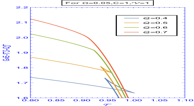
(b) We plot for the various values of $\mathcal{Q}$ for the fixed $\Omega$, $\mathcal{V}$ and $C$. For $\mathcal{Q}<\mathcal{Q}_{crit}$ (blue, orange) we can see a first-order phase transition. For $\mathcal{Q}=\mathcal{Q}_{crit}$ (green) there we see a second order phase transition and for $\mathcal{Q}>\mathcal{Q}_{crit}$(red), there are no phase transitions.

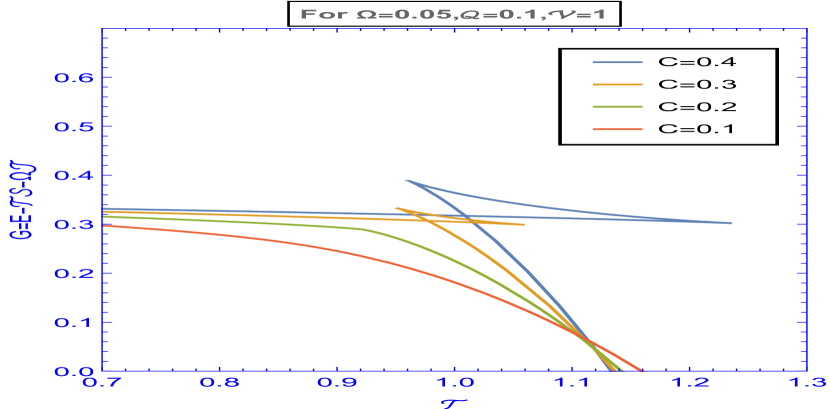
(c) We plot for the various values of $C$ for the fixed $\mathcal{Q}$, $\mathcal{V}$ and $\Omega$. For $C>C_{crit}$ (blue, orange) we can see a first-order phase transition. For $C=C_{crit}$ (green), we see a second-order phase transition and for $C<C_{Crit}$(red), there are no phase transitions.

Figure 2: Free energy $G$ vs. temperature $\mathcal{T}$ plot for the fixed $(\mathcal{Q},\Omega,\mathcal{V},C)$ ensemble in $d=4$

On the first plot, we have a plot (2(a)), the free energy function for the temperature for various values of $\Omega$. Here we see the picture as for $\Omega<\Omega_{crit}$ (blue, orange) for $\omega=\omega_{crit}$(green) and for $\Omega>\Omega_{crit}$ (red) while all for keeping $\mathcal{Q},C$ and $\mathcal{V}$ fixed. In this plot (2(a)) we see that the swallow tail is seen for $\Omega<\Omega_{crit}$, a kink-like figure for $\Omega=\Omega_{crit}$ and at last a smooth monotonous curve for $\Omega>\Omega_{crit}$. When $\mathcal{T}=0$ for all curves on plot (2(a)), as the temperature increases, the value of $\mathcal{S}$ also increases. we can see a low entropy stage, where the swallow tail is seen nearby $\mathcal{T}=0$. when it reaches the self-intersection point, it continues to have the lowest free energy. For large entropy $\mathcal{S}$ black holes are seen after crossing the self-intersection point, lying along the vertical branch, having the lowest free energy in the ensemble. For this range that is $\Omega<\Omega_{crit}$ we see the first order phase transition. As the value of $\omega$ increases, the swallow tail part is seen starting to vanish thereby remaining only a kink-like figure at $\Omega=\Omega_{crit}$. The plot at the critical point that is $(\Omega_{crit},\mathcal{T}_{crit})$ we see a second-order phase transition. For Plot (2(b)) we kind of see the same kind of pattern as seen in plot (2(a)). Here also we plot the free energy for temperature for different values of $\mathcal{Q}$.

For the second plot (2(b)), we kind of notice the same kind of pattern as seen in Plot (2(a)). Here we try to plot the free energy as a function of temperature for various values of charges namely $\mathcal{Q}<\mathcal{Q}_{crit}$ (blue, orange), $\mathcal{Q}=\mathcal{Q}_{crit}$ (green) and $\mathcal{Q}>\mathcal{Q}_{crit}$ (red) while we keep central charge $C$, CFT volume $\mathcal{V}$ and angular velocity $\Omega$ as constant or fixed. We see a "swallow-tail" behaviour for $\mathcal{Q}<\mathcal{Q}_{crit}$, a kink like structure for $\mathcal{Q}=\mathcal{Q}_{cirt}$ and then a smooth monotonous curve for $\mathcal{Q}>\mathcal{Q}_{crit}$. Starting from $\mathcal{T}=0$ for all the curves, the entropy $\mathcal{S}$ values increases along the curve as the value of $T$ increases. First, if we consider the swallowtail curve, only at near $\mathcal{T}=0$ we see a low entropy state and also having the minimum free energy $G$. It will continue to have low free energy as the temperature increases till it reaches the self-intersection point. After we cross this self-intersection point, the curves that are seen to be vertical for large $\mathcal{S}$ black holes which seem to be conjugate for the CFT states having higher entropy per degree of freedom, become the lowest state for free energy. We see a first-order phase transition at the self-intersection point between the low and high entropy for various values in the range $\mathcal{Q}<\mathcal{Q}_{crit}$. As the value of $\mathcal{Q}$ increases we can see that the swallow tail decreases till it reaches a kink for $\mathcal{Q}=\mathcal{Q}_{crit}$ and then for $\mathcal{Q}>\mathcal{Q}_{crit}$ we see a smooth curve.
We also have considered the changes in central charges $C$ which can be seen in plot (2(c)) while we keep $\mathcal{Q}$, $\Omega$ and $\mathcal{V}$ as fixed. We kind of note three different regimes namely $C<C_{crit}$ (red), $C=C_{crit}$ (green) and $C>C_{crit}$ (orange, blue). The third plot (2(c)) shows kind of same structure as plot (2(a)) and plot (2(b)) but a bit dissimilar is seen as they kind of show first-order phase transition for the low to high entropy degrees of freedom for the central charges in the ranges $C>C_{crit}$. We see a second order phase transition when $C=C_{crit}$ and last we see a single phase or we can say a smooth monotonous curve for $C<C_{crit}$. As we decrease the value of the central charge $C$ we notice that the "swallow-tail" behavior keeps on decreasing until $C$ reaches a critical kind of value which looks like a "kink" at the critical value after this we do not see any "swallow-tail" kind of structure.
If we kind of compare the three plots we see that the phase transition of first order occurs at $\Omega<\Omega_{crit}$ for plot (2(a)), $\mathcal{Q}<\mathcal{Q}_{crit}$ for plot (2(b)) and $C>C_{crit}$ for plot (2(c)).

3.3 Ensemble at fixed $(\varphi,\Omega,\mathcal{V},C)$

In this ensemble we kind of fix the angular velocity $\Omega$, the electric potential $\Phi$, the CFT volume $\mathcal{V}$, and the central charge $C$. We can derive the free energy as

and the temperature in this ensemble is given as

If we see the CFT first law (52), differentiating the free energy expression W (65), we get

$$dW=dE-\mathcal{T}d\mathcal{S}-\mathcal{S}d\mathcal{T}-\Omega d\mathcal{J}-\mathcal{J}d\Omega-\varphi d\mathcal{Q}-\mathcal{Q}d\varphi=-\mathcal{S}d\mathcal{T}-\mathcal{Q}d\varphi-pd\mathcal{V}+\mu dC-\mathcal{J}d\Omega$$ (67)

From the above equation (67) we can notice that the $W$ is kind of fixed at $(\mathcal{T},\varphi,\mathcal{V},C,\Omega)$. We see from the above equation (67) that the free energy behaves as a function of temperature $\mathcal{T}$ for the fixed values of $(\varphi,\Omega,\mathcal{V},C)$. For this ensemble given here, we can plot parametrically $W(\mathcal{T})$ for the entropy $\mathcal{S}$.

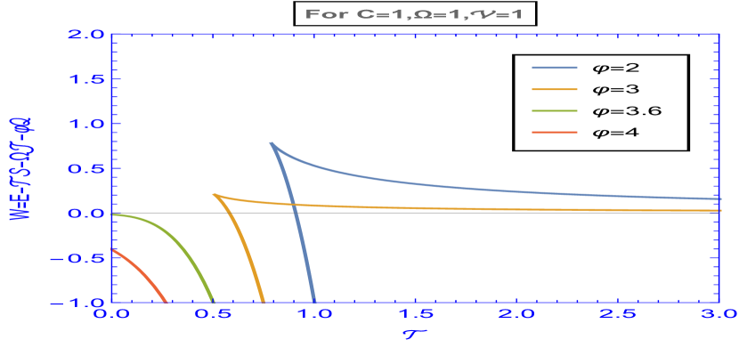
(a) We plot for various values of $\varphi$ keeping $C$, $\Omega$, $\mathcal{V}$ as constant. For $\varphi<\varphi_{crit}$ the free energy consists of two branches. At $W=0$, there is a first-order phase transition. For $\varphi\geq\varphi_{crit}$, the curve lies below $W=0$ and no phase transition takes place.

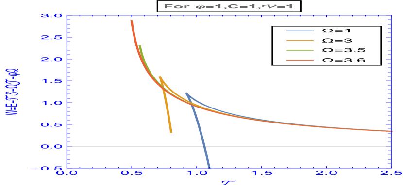
(b) We plot for the various vales of $\Omega$ while keeping $\varphi$, $C$ and $\mathcal{V}$ constant.For $\Omega<\Omega_{crit}$, the free energy consists of two branches. At $W=0$, there is a first-order phase transition. For $\Omega\geq\Omega_{crit}$ there is a single branch that lies above $W=0$ and has no phase transition.

(c) We plot for the various values of $\mathcal{V}$ keeping $\varphi$, $\Omega$, $C$. For $\mathcal{V}<\mathcal{V}$, the free energy consists of two branches. At $W=0$, there is a first-order phase transition. For $\mathcal{V}\geq\mathcal{V}_{crit}$ there is a single branch that lies above $W=0$ and has no phase transition.

Figure 3: Free energy $W$ vs. temperature $\mathcal{T}$ plot for the fixed ($\varphi$,$\Omega$,$\mathcal{V}$,C) ensemble in $d=4$ dimensions

From the expression of the free energy and temperature, we can plot the free energy $W(\mathcal{T})$ using the entropy $\mathcal{S}$ parametrically for the fixed value of $(\Omega,\varphi,\mathcal{V},C)$ as we can see in the Figure 3. In the plot (3(a)) we can see that the $W-\mathcal{T}$ displays a certain different kind of behavior above and below a certain critical value $\varphi_{crit}$. We see for the value of $\varphi\geq\varphi_{crit}$ (green, red), we can see that the free energy is a single-valued function as a function of temperature, where $W\leq 0$ and the curve cuts the $W$ axis. also for the value of $\varphi<\varphi_{crit}$ (orange, blue), we can see that the free energy curve consists of an upper or lower branch that meets at a cusp which actually corresponds to the low entropy (small black holes) and the high entropy states (large black holes) respectively.
We see that the blue and the orange curve change sign for the free energy at $W=0$ which corresponds to a first-order phase transition. When the free energy $W<0$ then the large - entropy which is termed as "deconfined" seems to be dominating. But when $W>0$, we see that the "confined state is more preferred." We note that the confinement/deconfinement phase transition is analogous to the generalized Hawking-Page phase transition between the AdS space containing thermal radiation and the large AdS black holes. We see that the Hawking-Page transition also exists for charged and rotating black holes which was originally discovered for AdS-Schwarzschild black holes.
We see the plot (3(b)) of figure 3 We can see the variation of the free energy $W$ with respect to $\mathcal{T}$ with the help of entropy $\mathcal{S}$ parametrically. We can note that for various values of $\Omega$, there is either a single-valued behavior of the free energy or a bifurcation point from where two sets of branches emerge. We can calculate the turning point or the cusp as

$$\left(\frac{\partial\mathcal{T}}{\partial S}\right)_{\varphi,\Omega,\mathcal{V},C}=0$$ (68)

which in turn gives the corresponding entropy and also the temperature of the turning point as( $S_{cusp}$, $\mathcal{T}(S_{cusp})$). From this equation, we get one of the solutions for $S_{cusp}$ as

$$S_{cusp}=-\frac{4\pi\left(C\mathcal{V}\varphi^{2}+4\pi C\right)}{4\pi-\Omega^{2}\mathcal{V}}$$ (69)

Therefore putting the value of $S_{cusp}$ (69) in the temperature (66), we get:-

How ever if we just simplify the equation (70), it reduces to zero. So from the $T(S_{cusp})$ we can extract that

$$4\pi-\mathcal{V}\Omega\leq 0\quad i.e\quad\Omega_{c}=\frac{2\sqrt{\pi}}{\sqrt{\mathcal{V}}}$$ (71)

Hence if the above condition satisfies then we can see a single-valued Gibbs free energy is obtained.

From the plot (3(c)) we also notice that there is a point where the free energy changes its sign. This does indicate phase transition where we know that when a system has a lower free energy it is a more thermodynamically preferred region. So we kind of say that when the temperature increases from zero of the CFT, in this ensemble the confined state is dominated until it reaches a turning point where the free energy $W$ changes its sign from a positive value to a negative value. There only the system is seen to have a first-order phase transition and after this, the system seems to be dominated by the de-confined state large entropy. This is kind of similar to the Hawking-Page transition.

3.4 Ensemble at fixed $(\varphi,\mathcal{J},\mathcal{V},C)$

In this ensemble we try to fix the electric potential $\varphi$, the angular velocity $\mathcal{J}$, CFT volume $\mathcal{V}$, and the central charge $C$. We can write the free energy as

$$X=E-\mathcal{T}\mathcal{S}-\varphi\mathcal{Q}$$ (72)

We will not be able to write down explicitly the free energy and temperature expressions as they are quite lengthy and complicated. From the CFT first law, we notice that from the free energy expression (52), we put the value in the result when differentiating (72), we get:-

$$dX=dE-\mathcal{T}d\mathcal{S}-\mathcal{S}d\mathcal{T}-\varphi d\mathcal{Q}-\mathcal{Q}d\varphi=-\mathcal{S}d\mathcal{T}-\mathcal{Q}d\varphi-pd\mathcal{V}+\mu dC$$ (73)

We see that the free energy $X$ (73) is a kind of fixed at $(\mathcal{T},\varphi,\mathcal{V},C,\Omega)$. We can note that the free energy $X$ behaves as a function of the temperature $\mathcal{T}$ for the various fixed values of $(\varphi,\mathcal{J},\mathcal{V},C)$. For this system, we can plot parametrically $X(\mathcal{T})$ by using the entropy $\mathcal{S}$. In the figure 5 we plot different values of $\mathcal{J}$ while keeping electric potential $\varphi$ and the central charge $C$ fixed.Also, we plot for various values of $C$ where we keep both $\varphi$ and $\mathcal{J}$ fixed. Also, we plot the graphs seen in Figure 5(a) for various values of $\varphi$ and keep $C$ and $\mathcal{J}$ fixed. We see a total of three cases is there for the plots showing the swallowtail behavior. But from the plots, we can notice one thing, this criticality occurs in $\mathcal{J}<\mathcal{J}_{crit}$, $\varphi<\varphi_{crit}$ for the angular momentum and electric potential case and for the central charge it occurs at $C>C_{crit}$.

(a) We plot for the various values of $\mathcal{J}$ for the fixed $\varphi$, $\mathcal{V}$ and $C$. For $\mathcal{J}<\mathcal{J}_{crit}$ (blue, orange) we can see a first-order phase transition. For $\mathcal{J}=\mathcal{J}_{crit}$ (green) there we see a second order phase transition and for $\mathcal{J}>\mathcal{J}_{crit}$(red), there are no phase transitions.

(b) We plot for the various values of $C$ for the fixed $\varphi$, $\mathcal{V}$ and $\mathcal{J}$. For $C<C_{crit}$ (blue, orange) we can see a first-order phase transition. For $C=C_{crit}$ (green) we see a second-order phase transition and for $C>C_{crit}$(red), there are no phase transitions.

Figure 4: Free energy F vs temperature $\mathcal{T}$ plot for fixed ($\varphi$,$\mathcal{J}$,$\mathcal{V}$,C) ensemble in $d=4$

For the first two cases which implies $\mathcal{J}$ and $C$, we see it in plot (4(a)) and (4(b)) and the the change in $\varphi$, we see it in plot (5(a))
On the first plot (4(a)), we see that the free energy is plotted for the temperature by using the entropy $\mathcal{S}$ parametrically for the various values of $\mathcal{J}$. Here we note that for the values where $\mathcal{J}<\mathcal{J}_{crit}$ (blue,orange), then for $\mathcal{J}=\mathcal{J}_{crit}$ (green) and lastly for $\mathcal{J}>\mathcal{J}_{crit}$ (red) while we keep $\varphi$, $C$ and $\mathcal{V}$ as constant. Here for the plot (4(a)), we see that a swallow-tail is generated for various values of $\mathcal{J}<\mathcal{J}_{crit}$, then a kink-like structure for $\mathcal{J}=\mathcal{J}_{crit}$ and then a smooth monotonous curve for various values of $\mathcal{J}>\mathcal{J}_{crit}$. We see that for all the curves when $\mathcal{T}=0$, when the temperature increases, the value for the entropy also increases. we can see at a low entropy range, it continues to have the lowest free energy when it reaches the self-intersection point. For the black holes having large entropy $\mathcal{S}$, it is noticed that the black hole after crossing the self-intersection point, the points lying along the vertical branch is seen to have the lowest free energy in the considered ensemble. For this range that is we see when $J<J_{crit}$, we kind of see a first-order phase transition. Now as the value of $\mathcal{J}$ increases, the swallow tail part of the curve is seen to vanish thereby now only remaining a kink-like structure at $\mathcal{J}=\mathcal{J}_{crit}$. The plot at the critical point $(\mathcal{J}_{crit},\mathcal{T}_{crit})$ is actually the second-order phase transition. For the plot (4(b)), we see the same kind of pattern as seen in the plot (4(a)). But there is a catch that we talk about below. We also plot the free energy $X$ with respect to the temperature for various values of $C$.
In the plot (4(b)) we note that we have considered the changes in central charges while we have kept the $\mathcal{J}$, $\varphi$ and $\mathcal{V}$ as fixed or we can say as constant. Here we seem to have three regions namely the regions where $C<C_{crit}$ (red), $C=C_{crit}$ (green), and $C>C_{crit}$ (orange, blue). This plot seems a bit different from the plot(4(a)) in that a dissimilarity occurs as they show the first-order phase transitions when the value of the central charges $C>C_{crit}$. Then we also see a second-order phase transition when the value of the central charge is $C=C_{crit}$ and at last the red curve which is the smooth monotonous curve is due to the central charge when the value is $C<C_{crit}$. As we decrease the value of the central charge, we notice that the swallow-tail behavior tends to decrease until $C$ reaches a kind of critical value which looks like a kink at the critical value after which we do not see any kind of swallow tail kind of structure.

(a) We plot for the various values of $\varphi$ for the fixed $\mathcal{J}$, $\mathcal{V}$ and $C$. Here for all the plots $\varphi<\varphi_{crit}$

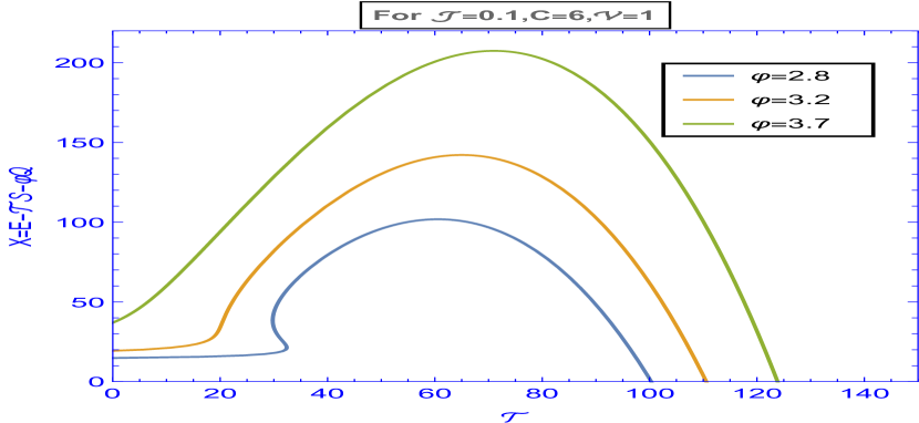
(b) We plot for the various values of $\varphi$ for the fixed $C$, $\mathcal{V}$ and $\mathcal{J}$. Blue plot corresponds to $\varphi<\varphi_{crit}$. Orange plot corresponds to $\varphi=\varphi_{crit}$ and green plot corresponds to $\varphi>\varphi_{crit}$

Figure 5: Free energy F vs temperature $\mathcal{T}$ plot for fixed ($\varphi$,$\mathcal{J}$,$\mathcal{V}$,C) ensemble in $d=4$

For plot (5(a)) and (5(b)), we plot the free energy for the temperature parametrically with entropy for various values of $\mathcal{J}$, $C$, $\varphi$ and $\mathcal{V}$. We see for plot (5(a)), by keeping $\mathcal{J}$, $C$ and $\mathcal{V}$ constant, we plot for various values of $\varphi$. Here in this plot, we notice three phases for all the values of $\varphi$. For plot (5(b)), we plot for similar values of $\mathcal{J}$, $C$ and $\mathcal{V}$, but different values of $\varphi$. Here we get three plots where for the blue plot ($\varphi<\varphi_{crit}$) we get three phases and then for the orange and green plot ($\varphi\geq\varphi_{crit}$), we get only one phase.

4 Other ensembles

In the previous sections we have discussed certain ensembles and their free energy namely for fixed $(\mathcal{Q},\mathcal{J},\mathcal{V},C)$, fixed $(\mathcal{Q},\Omega,\mathcal{V},C)$, fixed $(\varphi,\Omega,\mathcal{V},C)$ and lastly fixed $(\varphi,\mathcal{J},\mathcal{V},C)$ ensembles. Now in addition to all these ensembles we also have taken 6 more ensembles, precisely the p ensembles, and one ensemble taking all the dependent variables as seen below from $F_{1}-F_{6}$ namely

$$\begin{split}&\text{fixed}\quad(\mathcal{Q},\mathcal{J},p,C):\quad F_{1}=E-\mathcal{T}\mathcal{S}+p\mathcal{V}=\varphi\mathcal{Q}+\Omega\mathcal{J}+\mu C+p\mathcal{V}\\ &\text{fixed}\quad(\mathcal{Q},\Omega,p,C):\quad F_{2}=E-\mathcal{T}\mathcal{S}-\Omega\mathcal{J}-p\mathcal{V}=\varphi\mathcal{Q}+\mu C+p\mathcal{V}\\ &\text{fixed}\quad(\varphi,\mathcal{J},p,C):\quad F_{3}=E-\mathcal{T}\mathcal{S}-\varphi\mathcal{Q}-p\mathcal{V}=\Omega\mathcal{J}+\mu C+p\mathcal{V}\\ &\text{fixed}\quad(\varphi,\Omega,p,C):\quad F_{4}=E-\mathcal{T}\mathcal{S}-\varphi\mathcal{Q}-\Omega\mathcal{J}-p\mathcal{V}=\mu C+p\mathcal{V}\\ &\text{fixed}\quad(\mathcal{Q},\mathcal{J},p,\mu):\quad F_{5}=E-\mathcal{T}\mathcal{S}-\mu C+p\mathcal{V}=\varphi\mathcal{Q}+\Omega\mathcal{J}+p\mathcal{V}\\ &\text{fixed}\quad(\varphi,\Omega,\mathcal{V},\mu):\quad F_{6}=E-\mathcal{T}\mathcal{S}-\varphi\mathcal{Q}-\varphi\mathcal{J}-\mu C=0\end{split}$$ (74)

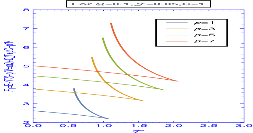
(a) Plot 1

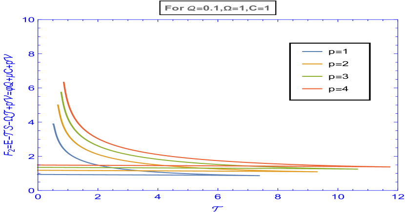
(b) Plot 2

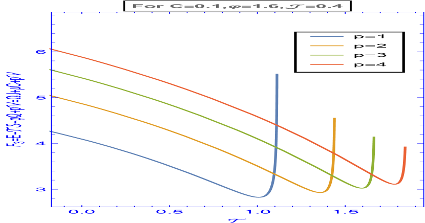
(c) Plot 3

(d) Plot 4

(e) Plot 5

Figure 6: These other ensembles are plotted for the temperature for $d=4$ dimensions corresponding to the ensembles at fixed $(\mathcal{Q},\mathcal{J},p,C)$, fixed $(\mathcal{Q},\Omega,p,C)$, fixed $(\varphi,\mathcal{J},p,C)$, fixed $(\varphi,\Omega,p,C)$, and for fixed $(\mathcal{Q},\mathcal{J},p,\mu)$ respectively (left to right)

In the figure 6, we have seen that the free energy is being plotted against the temperature for the first five ensembles for some constant parameter values. The top part from left to right are the fixed $(\mathcal{Q},\mathcal{J},p,C)$, $(\mathcal{Q},\Omega,p,C)$, $(\varphi,\mathcal{J},p,C)$ and the bottom two from left to right are given as $(\varphi,\Omega,p,C)$ and $(\mathcal{Q},\mathcal{J},p,\mu)$. We have not plotted here for the $(\varphi,\Omega,\mathcal{V},\mu)$ ensemble because the associated free energy $F_{6}$ is seen to be as zero that is $(F_{6}\equiv 0)$ due to the Euler equation expansion.
Certain things we can note from Figure 6 is that all the five ensembles do not display any kind of critical phenomena or phase transitions. Therefore we can say that we do not see any critical behavior in the ensembles taken or to be precise the $p-\mathcal{V}$ criticality in the fixed p ensembles for the thermal states or the CFT. Further in the three ensembles at fixed $(\mathcal{Q},\mathcal{J},\mathcal{V},C)$, $(\mathcal{Q},\Omega,\mathcal{V},C)$ and $(\mathcal{Q},\mathcal{J},p,\mu)$, we observe two branches in the free energy plots: the lower branch corresponds to a state with a low value of $S/C$ which associates to the small type of ADS black holes and the upper branch corresponds to the high value of $S/C$ which corresponds to the large type of AdS black holes. The lower branch has the least free energy and hence this phase is dominating in this respective ensembles.

5 Conclusion

In the beginning, we review very briefly the the mass-energy formulas for the extended phase space thermodynamics, then for the mixed thermodynamics, and lastly for the CFT thermodynamics for the Kerr-Newman AdS black hole comprising both the charge and rotating element dd ; ii ; dd1 . Then we investigated the various phase transitions for the dual holographic CFT states for the Kerr-Newman AdS black hole taking in various ensembles. Note that we were not able to take the entire ensemble as the interplay between the $(\mathcal{J},\Omega)$ and $(\mathcal{Q},\varphi)$ is quite complex, so we could only investigate a few ensembles. In the ensemble $(\mathcal{Q},\mathcal{J},\mathcal{V},C)$ in section 3.1 we have plotted the free energy $F$ for the temperature parametrically with the entropy $\mathcal{S}$. We have plot three different plots seen in Figure 1 that we plot for various values of electric charge $\mathcal{Q}$ when keeping the $\mathcal{J}$, $\mathcal{V}$ and the central charge $C$ as constant. For this, we have observed a first-order phase transition for the range of $\mathcal{Q}<\mathcal{Q}_{crit}$. For when $\mathcal{Q}=\mathcal{Q}_{crit}$, we observe a kink-like structure which is described as a second-order phase transition. At last, for $\mathcal{Q}>\mathcal{Q}_{crit}$ we see a smooth monotonous curve and there is no swallowtail or a kink anywhere. Now when we plot various values of $\mathcal{J}$, we get a first-order phase transition which is represented by a swallowtail for the range of angular momentum when $\mathcal{J}<\mathcal{J}_{crit}$ and then a second order phase transition for the value when $\mathcal{J}=\mathcal{J}_{crit}$ and it is visualized as a kink like structure and then we observe a smooth curve for the value of $\mathcal{J}$ when $\mathcal{J}>\mathcal{J}_{crit}$. Lastly, for this ensemble we plot for the various values of the central charge $C$, keeping $\mathcal{J}$, $\mathcal{Q}$, and $\mathcal{V}$ constant. When $C>C_{crit}$ we get the swallow tail-like structure which is the first-order phase transition at the point when the vertical line cuts the horizontal line. For $C=C_{crit}$, we get the second order phase transition which is seen as a kink, and then a smooth monotonous curve for the central charge range that is $C<C_{crit}$
Now for the ensemble $(\mathcal{Q},\Omega,\mathcal{V},C)$ in section 3.2, we also have plotted the $G(\mathcal{T})$ graph for various values and have obtained three plots seen in Figure 2. Firstly we have plotted for various values of $\Omega$, keeping $\mathcal{Q}$, $\mathcal{V}$ and $C$ as constant. For this then we get a swallowtail-like structure when the value of $\Omega$ is $\Omega<\Omega_{crit}$. This is also called the first-order phase transition. Now when $\Omega=\Omega_{crit}$ we get a kink-like structure that corresponds to the second-order phase transition and then for $\Omega>\Omega_{crit}$ we get a smooth monotonous curve. Now when we plot for the various values of $\mathcal{Q}$ with various values as constant namely $\Omega$, $\mathcal{V}$ and $C$, we see a first-order phase transition for when $\mathcal{Q}<\mathcal{Q}_{crit}$ which is seen as a swallow tail structure. Then when $\mathcal{Q}=\mathcal{Q}_{crit}$ we see a kink-like structure which is second order phase transition and then when $\mathcal{Q}>\mathcal{Q}_{crit}$ we get a smooth curve like structure. Now for this ensemble if we plot the curve for various values of the central charge $C$ for constant values of $\mathcal{Q}$, $\Omega$, and $\mathcal{V}$. We get the first order phase transition for $C>C_{crit}$ which we see a swallowtail behavior. Then for $C=C_{crit}$, we get the second-order phase transition which also visually looks like a kink. and then lastly for $C<C_{crit}$ we get a smooth monotonous curve.
In the ensemble $(\varphi,\Omega,\mathcal{V},C)$ of section 3.3, we have plotted the $W(\mathcal{T})$ plot parametrically with entropy. When we plot the various values of $\varphi$ while keeping the other parameters $\Omega$, $\mathcal{V}$ and $C$ as constant. We notice that for $\varphi>\varphi_{crit}$, the free energy plot is single-valued where $W\leq 0$ and the curve cuts the $W$ axis. Now for the value of $\varphi<\varphi_{crit}$, we notice that the free energy curve consists of an upper and lower branch. For this branch, it changes sign at $W=0$ which is the first order phase transition. When $W<0$ it is said to be deconfined and when $W>0$, it is said to be confined. Now when we plot for various values of $\omega$, there is a single value behavior of the Gibbs free energy and then there we see a bifurcation point where two branches appear. When the temperature increases from zero of the CFT, the ensemble in the confined state is dominated until we get a turning point where the free energy changes sign. Here only the first-order phase transition takes place. We can see the same kind of analogy when we plot for various values of $\mathcal{V}$. We also note that the (de)confinement phase transition does not depend on the central charge as we get no point where we get a single phase so the phase transition means that $\Omega$ and $\varphi$ depend on the CFT volume.

Now, section 3.4, in the ensemble $(\varphi,\mathcal{J},\mathcal{V},C)$, we have parametrically plot the $X(\mathcal{T})$ curve with the help of the entropy $\mathcal{S}$. Now when we have plotted for various values of $\mathcal{J}$, while having certain parameters constant like $\varphi$, $\mathcal{V}$, $C$. Here for $\mathcal{J}<\mathcal{J}_{crit}$ we see a swallow tail-like structure which is the first order phase transition. Then we see a second-order phase transition which looks like a kink and is at the value where $\mathcal{J}=\mathcal{J}_{crit}$. Then when the value of $\mathcal{J}>\mathcal{J}_{crit}$ we see a smooth curve-like structure. Now then for various values of $C$ keeping the $\varphi$, $\mathcal{V}$ and $C$ as constant. Here we have seen a first-order phase transition that is a swallowtail-like structure when the value of the central charge is $C>C{crit}$. Then a second-order phase transition at the kink when $C=C_{crit}$. and then a smooth monotonous curve when $C<C_{crit}$ where we see no phase transition. Now when we plot for various values of $\varphi$, we get the threee phases for all the values of $\varphi$. When $\varphi<\varphi_{crit}$, we see three phases and when $\varphi\geq\varphi_{crit}$, we get only one phase.
We also plot for the various $p$ ensembles in section 4. For six ensembles we examine the phase transition but we only get for five since the free energy for the fixed ($\varphi,\Omega,\mathcal{V},\mu$) ensemble gives zero $(F_{6}=0)$. So, for the remaining five ensembles, the plot didn’t show any kind of criticality or phase transitions. So there is no $p-\mathcal{V}$ criticality for the fixed $p$ ensembles for the thermal states or the CFT. The CFT phase transition of charged and rotating black holes matches to some extend to the charged black hole and rotating black hole. This type of behaviour shows that there should be some underlying universality in the phase transitions by using the AdS/CFT formalism.

In future endeavors, one can also examine the charge and rotating black holes in a more generalized form where we can also include the $\mu$ containing ensembles that were not included in this paper. One can also study more in-depth for each ensemble and check their coexistence plots, and specific heat. We can also extend the study to a different formalism, namely the RPST (restricted phase space thermodynamics). We can also examine thermodynamic topology by studying the phase transitions of various ensembles taken in this paper.

References

• (1) S. W. Hawking, Gravitational radiation from colliding black holes, Phys. Rev. Lett. 26, 1344-1346 (1971) doi:10.1103/PhysRevLett.26.1344
• (2) S. W. Hawking, Black hole explosions, Nature 248, 30-31 (1974) doi:10.1038/248030a0
• (3) S. W. Hawking, Particle Creation by Black Holes, Commun. Math. Phys. 43, 199-220 (1975) [erratum: Com mun. Math. Phys. 46, 206 (1976)] doi:10.1007/BF02345020
• (4) J. M. Bardeen, B. Carter, S. W. Hawking, The four laws of black hole mechanics, Commun. Math. Phys. 31 (1973) 161-170
• (5) J.D. Berkenstein, Black holes and entropy, Phys. Rev. D 7 (1973) 2333 [INSPIRE].
• (6) R. M. Wald, Entropy and black-hole thermodynamics, Phys. Rev. D 20, 1271-1282 (1979) doi:10.1103/PhysRevD.20.1271
• (7) Jacob D Bekenstein. Black-hole thermodynamics, Physics Today, 33(1):24–31, 1980.
• (8) R. M. Wald, The thermodynamics of black holes, Living Rev. Rel. 4, 6 (2001) doi:10.12942/lrr-2001-6 [arXiv:gr-qc/9912119 [gr-qc]].
• (9) S.Carlip, Black Hole Thermodynamics, Int. J. Mod. Phys. D 23, 1430023 (2014) doi:10.1142/S0218271814300237 [arXiv:1410.1486 [gr-qc]].
• (10) A.C.Wall, A Survey of Black Hole Thermodynamics, [arXiv:1804.10610 [gr-qc]].
• (11) P.Candelas and D.W.Sciama, Irreversible Thermodynamics of Black Holes, Phys. Rev. Lett. 38, 1372-1375 (1977) doi:10.1103
• (12) A. Chamblin, R. Emparan, C. V. Jhonson and R. C. Myers, Charged AdS black holes and catastrophic holography, Phys. Rev. D 60 (1999) 064018 [hep-th/9902170] [INSPIRE].
• (13) S.W. Hawking and D. N. Page, Thermodynamics of black holes in Anti-de Sitter space, Commun. Math. Phys. 87 (1983) 577 [INSPIRE].
• (14) A. Chamblin, R. Emparan, C. V. Jhonson and R. C. Myers, Holography, thermodynamics and fluctuations of charged AdS black holes, Phys. Rev. D 60 (1999) 104026 [hep-th/9904197] [INSPIRE].
• (15) Chao Wang, Bin Wu, Zhen Ming Xu, Wen Li Yang, Thermodynamic geometry of the RN-AdS black hole and non-local observables,[arXiv:2210.08718 ]
• (16) Yuchen Huang, Jun Tao, Peng Wang, Shuxuan Ying, Phase transitions and thermodynamic geometry of a Kerr-Newman black hole in a cavity, Eur.Phys.J.Plus 138, 265 (2023)[https://doi.org/10.1140/epjp/s13360-023-03858-w]
• (17) Wen-Xiang Chen, Yao-Guang Zheng, Thermodynamic geometric analysis of BTZ black hole under f(R) gravity, [arXiv:2112.15032 ]
• (18) Peng Wang, Feiyu Yao, Thermodynamic Geometry of Black Holes Enclosed by a Cavity in Extended Phase Space, Nulc. Phys. B, 976 (2022) 115715 [https://doi.org/10.1016/j.nuclphysb.2022.115715]
• (19) Amin Dehyadegari, Ahmad Sheykhi, Thermodynamic geometry and phase transition of spinning AdS black holes, Phys. Rev. D, 104, 104066, (2021) [doi:10.1103/PhysRevD.104.104066]
• (20) Shao-Wen Wei, Yu-Xiao Liu General thermodynamic geometry approach for rotating Kerr anti-de Sitter black holes, Phys. Rev. D, 104, 084087 (2021) [10.1103/PhysRevD.104.084087]
• (21) Seyed Ali Hosseini Mansoori, Thermodynamic geometry of the novel 4-D Gauss Bonnet AdS Black Hole, Phys.Dark Univ., 31 (2021) 100776 [doi:10.1016/j.dark.2021.100776]
• (22) Aritra Ghosh, Chandrasekhar Bhamidipati, Thermodynamic geometry for charged Gauss-Bonnet black holes in AdS spacetimes, Phys. Rev. D 101, 046005 (2020),[doi:10.1103/PhysRevD.101.046005]
• (23) Shao-Wen Wei and Yu-Xiao Liu. Topology of black hole thermodynamics., Phys. Rev. D 105:104003, (2022).
• (24) Shao-Wen Wei, Yu-Xiao Liu, and Robert B. Mann. Black hole solutions as topological thermodynamic defects. Phys. Rev. Lett., 129:191101,(2022).
• (25) B. Hazarika and P. Phukon, Thermodynamic topology of black Holes in f(R) gravity, Progress of Theoretical and Experimental Physics 4(2024), https://doi.org/10.1093/ptep/ptae035 [arXiv:2401.16756 [hep-th]].
• (26) N. J. Gogoi and P. Phukon, Thermodynamic topology of 4D Euler-Heisenberg-AdS black hole in different ensembles,[arXiv:2312.13577 [hep-th]]
• (27) B. Hazarika and P. Phukon, Thermodynamic Topology of $D=4,5$ Horava Lifshitz Black Hole in Two Ensembles,[arXiv:2312.06324 [hep-th]].
• (28) B. Hazarika, N. J. Gogoi and P. Phukon, Revisiting thermodynamic topology of Hawking-Page and Davies type phase transitions,[arXiv:2404.02526 [hep-th]].
• (29) D. Kastor, S. Ray and J. Traschen, Enthalphy and the mechanics of AdS black holes, Class. Quant. Grav. 26 (2009) 195011 [arXiv:0904.2765] [INSPIRE].
• (30) B.P. Dolan, The cosmological constant and the black hole equation of state, Class. Quant. Grav. 28 (2011) 125020 [arXiv:1008.5023] [INSPIRE].
• (31) B.P. Dolan, Pressure and volume in the first law of black hole thermodynamics, Class. Quant. Grav. 28 (2011) 235017 [arXiv:1106.6260] [INSPIRE].
• (32) M. Cvetic, G. W. Gibbons, D. Kubiznak and C.N. Pope, Black hole enthalphy and an Entropy Inequality for the Thermodynamic Volume, Phys. Rev. D 84 (2011) 024037 [1012.2888]
• (33) J.M. Maldacena, The large N limit of superconformal field theories and supergravity, Int. J. Theor. Phys. 43 (1999) 1113 [Adv. Theor. Math. Phys. 43 (1998) 231] [hep-th/971120][INSPIRE].
• (34) S. S. Gubser, I. R. Klebanov and A. M. Polyakov,Gauge Theory Correlators from Non-Critical String Theory, Phys. Lett. B 428, 105-114 (1998) doi:10.1016/S0370 2693(98)00377-3 [arXiv:hep-th/9802109 [hep-th]].
• (35) E. Witten, Anti-de Sitter space, thermal phase transition, and confinement in gauge theories, Adv. Theor. Math. Phys. 2 (1998) 505 [hep-th/9803131] [INSPIRE].
• (36) M. Cvetič and S.S. Gubser, Phases of R charged black holes, spinning branes and strongly coupled gauge theories, JHEP 04 (1999)024 [hep-th/9902195] [INSPIRE].
• (37) D. Kubiznak and R.B. Mann, P-V criticality of charged AdS black holes, JHEP 07 (2012)033 [arXiv:1205.0559] [INSPIRE].
• (38) S. Gunasekaran, R. B. Mann and D. Kubiznak, Extended phase space thermodynamics for charged and rotating black holes and Born-Infels vacuum polarization JHEP 11 (2012) 110 [1208.6251]
• (39) S.-W. Wei, P. CHeng and Y.-X. Liu, Analytical and exact critical phenomena of d-dimensional singly spinning Kerr-AdS black holes Phys. Rev. D 93 (2016) 084015 [1510.00085]
• (40) P. Cheng, S.-W. Wei and Y.-X. Liu, Critical phenomena in the extended phase space of Kerr-Newman-AdS black holes Phys. Rev. D 94 (2016) 024025 [1603.08694].
• (41) D. Kubiznak, R.B. Mann and M. Teo, Black hole chemistry: thermodynamics with Lambda, Class. Quant. Grav. 34 (2017) 063001 [arXiv:1608.06147] [INSPIRE].
• (42) B.P. Dolan, A. Kostouki, D. Kubiznak and R.B. Mann, Isolated critical point from Lovelock gravity, Class. Quant. Grav. 31 (2014)242001 [arXiv:1407.4783] [INSPIRE]
• (43) R.A. Hennigar, R.B. Mann and E. Tjoa, Superfluid black holes, Phys. Rev. Lett. 118 (2017) 021301 [arXiv:1402.2837] [INSPIRE].
• (44) N. Altamirano, D. Kubiznak, R.B. Mann and Z. Sherkatghanad, Kerr-AdS analogue of triple point and solid/liquid/gas phase transition, Class. Quant. Grav. 31 (2014)042001 [arXiv:1308.2672] [INSPIRE].
• (45) S.-W. Wei and Y.-X. Liu, Triple points and phase diagrams in the extended phase of charged Gauss-Bonnet black holes in AdS space, Phys. Rev. D 90 (2014)044057 [arXiv:1402:2837] [INSPIRE].
• (46) A.M. Frassino, D. Kubiznak, R.B. Mann and F. Simovic, Multiple reentrant phase transitions and triple points in Lovelock thermodynamics, JHEP 09 (2014)080 [arXiv:1406.7015] [INSPIRE].
• (47) N Altamirano, D. Kubiznak and R.B. Mann, Reentrant phase transition in rotating Anti-de Sitter black holes, Phys. Rev. D 88 (2013)101502 [arXiv:1306.5756] [INSPIRE].
• (48) S.-W. Wei, Y.-X. Liu and R. B. Mann, Respulsive Interactions and Universal Properties of Charged Anti-de Sitter Black Hole Microstructures, Phys. Rev. Lett. 123 (2019) 071103 [1906.10840]
• (49) M. Tavakoli, J. Wu and R. B. Mann, Multi-critical points in black hole phase transitions, JHEP 12 (2022) 117 [2207.03505]
• (50) J. Wu and R. B. Mann, Multicritical Phase Transitions in Lovelock AdS Black Holes, 2212.08087
• (51) M.R. Visser, Holographic thermodynamics requires a chemical potential for color, Phys. Rev. D 105 (2022) 106014 [arXiv:2101.04145] [INSPIRE].
• (52) R. B. Alfaia, I. P. Lobo, L. C. T. Brito, Central charge criticality of charged AdS black hole surrounded by different fluids, Eur. Phys. J. Plus 137 (2022) 402 [arXiv:2109.06599 ] [hep-th]
• (53) A. M. Frassino, J. F. Pedraza, A. Svwsko and M. R. Visser, Higher-Dimensional Origin of Extended Black Holes Thermodynamics, Phys. Rev. Lett. 130 (2023) 161501 [2212.14055].
• (54) D. Sarkar and M. Visser, The first law of differential entropy and holographic complexity, JHEP 11 (2020) 004 [arXiv:2008.12673] [INSPIRE]
• (55) D. Kastor, S. Ray and J. Traschen, , Chemical potential in the first law for holographic entanglement entropy, JHEP 11 (2014) 120 [arXiv:1409.3521] [INSPIRE].
• (56) D. Kastor, S. Ray and J. Traschen, Smarr formula and an extended first law for Lovelock gravity, Class. Quant. Grav. 27 (2010) 235014 [arXiv:1005.5053] [INSPIRE].
• (57) B.P. Dolan, Bose condensation and branes, JHEP 10 (2014) 179 [arXiv:1406.7267] [INSPIRE].
• (58) J.-L. Zhang, R.-G. Cai and H. Yu, Phase transition and thermodynamical geometry for Schwarzschild AdS black hole in $AdS^{5}$ × $S_{5}$ spacetime, JHEP 02 (2015) 143 [arXiv:1409.5305] [INSPIRE].
• (59) A. Karch and B. Robinson, Holographic black hole chemistry, JHEP 12 (2015) 073 [arXiv:1510.02472] [INSPIRE].
• (60) G. Zeyuan and L. Zhao, Restricted phase space thermodynamics for AdS black holes via holography, Class. Quant. Grav. 39 (2022) 075019 [arXiv:2112.02386] [INSPIRE].
• (61) T. Wang and L. Zhao, Black hole thermodynamics is extensive with variable Newton constant, Phys. Lett. B 827 (2022) 136935 [arXiv:2112.11236] [INSPIRE].
• (62) I.P. Lobo, J.P. Morais Graça, E. Folco Capossoli and H. Boschi-Filho, A varying gravitational constant map in asymptotically AdS black hole thermodynamics, Phys. Lett. B 835 (2022) 137559 [arXiv:2206.13664] [INSPIRE].
• (63) W. Cong, D. Kubiznak and R.B. Mann, Thermodynamics of AdS Black Holes: Critical Behaviour of Central Charge, Phys. Rev. Lett. 127 (2021) 091301 [2105.02223]
• (64) N. Kumar, S. Sen and S. Gangopadhyay, Breaking of the universal nature of the central charge criticality in AdS black holes in Gauss-Bonnet gravity, Phys. Rev. D 107 (2023) 046005 [2211.00925].
• (65) Y. Qu, J. Tao and H. Yang, Thermodynamics and phase transition in central charge criticality of charged Gauss-Bonnet AdS black holes, 2211.08127
• (66) N. Kumar, S. Sen and S. Gangopadhyay, Phase transition structure and breaking of universal nature of central charge criticality in a Born-Infeld AdS black hole, Phys. Rev. D 106 (2022) 026005 [2206.00440]
• (67) N.-C. Bai, L. Song and J. Tao, Reentrant phase transition in holographic thermodynamics of Born-Infeld AdS black hole, 2212.04341
• (68) W. Cong, D. Kubiznak, R. B. Mann and M. R. Visser, Holographic CFT phase transitions and criticality for charged AdS black holes, JHEP 08 (2022) 174 [2112.14848]
• (69) T.-F. Gong,J. Jiang, M. Zhang, Holographic thermodynamics of rotating black holes, JHEP, 105 (2023) [arXiv:2305.00267]
• (70) Ahmed, M.B., Cong, W., Kubizňák, D. et al. Holographic CFT phase transitions and criticality for rotating AdS black holes J. High Energ. Phys.2023, 142 (2023).https://doi.org/10.1007/JHEP08(2023)142
• (71) M.M. Caldarelli, G. Cognola and D. Klemm, Thermodynamics of Kerr-Newman-AdS black holes and conformal field theories, Class. Quant. Grav. 17 (2000) 3999 [hep-th/9908022] [INSPIRE].
• (72) N. Altamirano, D. Kubiznak, R.B. Mann and Z. Sherkatghanad, Kerr-AdS analogue of triple point and solid/liquid/gas phase transition, Class. Quant. Grav. 31 (2014)042001 [arXiv:1308.2672] [INSPIRE].
• (73) N Altamirano, D. Kubiznak and R.B. Mann, Reentrant phase transition in rotating Anti-de Sitter black holes, Phys. Rev. D 88 (2013)101502 [arXiv:1306.5756] [INSPIRE].
• (74) S.-J. Yang, R. Zhou, S.-W. Wei and Y.-X. Liu, Kinetics of a phase transition for a Kerr-AdS black hole on the free -energy landscape, Phys. Rev. D 105 (2022) 084030 [2105.00491]
• (75) S.S. Gubser, I.R. Klebanov and A.M. Polyakov, Gauge theory correlators from noncritical string theory, Phys. Lett. B 428 (1998) 105 [hep-th/9802109] [INSPIRE].
• (76) E.Witten, Anti-de Sitter space and holography, Adv. Theor. Math. Phys.2(1998) 253 [hepth-/9802150][INSPIRE]
• (77) M.B. Ahmed et al., Holographic Dual of Extended Black Hole Thermodynamics, Phys. Rev. Lett. 130 (2023) 181401 [arXiv:2302.08163] [INSPIRE].
• (78) I. Savonije and E.P. Verlinde, CFT and entropy on the brane, Phys. Lett. B 507 (2001) 305 [hep-th/0102042] [INSPIRE].