Online Time-Informed Kinodynamic Motion Planning of Nonlinear Systems

Abstract

Sampling-based kinodynamic motion planners (SKMPs) are powerful in finding collision-free trajectories for high-dimensional systems under differential constraints. Time-informed set (TIS) can provide the heuristic search domain to accelerate their convergence to the time-optimal solution. However, existing TIS approximation methods suffer from the curse of dimensionality, computational burden, and limited system applicable scope, e.g., linear and polynomial nonlinear systems. To overcome these problems, we propose a method by leveraging deep learning technology, Koopman operator theory, and random set theory. Specifically, we propose a Deep Invertible Koopman operator with control U model named DIKU to predict states forward and backward over a long horizon by modifying the auxiliary network with an invertible neural network. A sampling-based approach, ASKU, performing reachability analysis for the DIKU is developed to approximate the TIS of nonlinear control systems online. Furthermore, we design an online time-informed SKMP using a direct sampling technique to draw uniform random samples in the TIS. Simulation experiment results demonstrate that our method outperforms other existing works, approximating TIS in near real-time and achieving superior planning performance in several time-optimal kinodynamic motion planning problems.

I INTRODUCTION

Sampling-based motion planning methods are known for rapidly finding collision-free “geometric” paths from a start to a goal point in high-dimensional C-space. The popular RRT [1] grows a tree structure by drawing random samples until reaching the goal, guaranteeing probabilistic completeness. Its optimal version, RRT^∗ [2], provides the property of asymptotic optimality, whereas it costs too much time due to a uniform sampling strategy in the whole C-space [3, 4]. To speed up the convergence to the optimal solution, some heuristic sampling approaches have been proposed; for example, “$L_{2}$ Informed Set” containing all the potential shorter solutions is constructed to restrict the subsequent searches after an initial path is found [5].

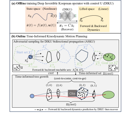
Figure 1: An illustration of online time-informed kinodynamic motion planning of nonlinear control systems. (a) A Deep Invertible Koopman operator with control U model, DIKU, is trained offline for the nonlinear systems to obtain equivalent linear systems that enable forward and backward dynamics prediction in the lifted space. (b) Our algorithm randomly samples states in the start and goal sets. It then uses the ASKU to bidirectionally propagate the learned linear dynamics and then recover, generating the forward reachable set $\mathcal{X}_{k}^{f}$ (independent blue dashed convex hull) and backward reachable tube $\mathcal{X}^{b}_{-cost:0}$ (serials of green dashed convex hulls) in near real-time. Their intersections constitute the time-informed set (TIS) $\Omega(cost)$ (black convex polygons). Time-informed tree growth is achieved for the off-the-shelf SKMPs by directly sampling in the TIS. The TIS updates according to the cost of the search tree returned after sufficient iterations to help refine the solution (red line).

When kinodynamic constraints, i.e., kinematic and differential constraints, are considered, the problem becomes PSPACE-hard and imposes a heavy computational burden. Optimal trajectories under kinodynamic constraints, instead of line segments, connecting any two intermediate tree nodes are required to form the edges of the tree. Local trajectory optimization solvers [6, 7] and random shooting methods [8, 1] are widely implemented to solve this two-point boundary value problem (TPBVP). Stable Sparse RRT (SST) [8] performs forward dynamic simulation with randomly sampled control signals for steering, eliminating the need for TPBVP solvers. Nevertheless, it is computation-demanding since its unbiased exploration of the whole state space. Hierarchical rejection sampling (HRS) [9] and Markov Chain Monte-Carlo (MCMC) [10] algorithms were proposed to generate samples within the informed set of non-Euclidean state spaces. However, the HRS method takes a longer time as the interested subspace shrinks or in high-dimensional space. Although the Hit-and-Run (HNR) MCMC method [10] is efficient, it requires an initial solution and applies to only certain systems for minimum-time problems.

Reachability-guided methods have been proposed to reduce computation cost [11]. At each extension, the polytopic forward reachable set (FRS) of each state is approximated to avoid selecting the nearest but unreachable state [12]. In addition, the TIS that includes all feasible kinodynamic trajectories is provided to restrict the sampling domain [13]. In principle, a set operation of the FRS of the start and the backward reachable tube (BRT) of the goal state is conducted. Tang et al. [14], which is most relevant to ours, relaxed the Hamilton-Jacobi-Bellman (HJB) equation to compute a modified TIS, broadening the system scope from linear [13] to polynomial nonlinear (PNL) systems and conducting a heuristic search from the beginning. However, it suffers from the curse of dimensionality, a heavy computational burden, and limited system-specific applicable scope. The sampling-based reachability analysis method that takes convex hulls for propagated states with random control inputs from the start has great potential to solve these problems by leveraging random set theory [15]. However, only FRSs can be approximated since there is no generic differential equation for the backward propagation of nonlinear systems. Considering Deep Koopman Operator (DKO) can predict the forward evolution of nonlinear dynamics by mapping the original system into an equivalent linear one in an observation space via deep neural network (DNN) [16] and linear systems are invertible, we integrate it into the sampling-based method to pave the path of constructing BRT. Furthermore, an adversarial sampling manner can guarantee the over-approximation reachability analysis, benefiting informed sampling. Although reachable tubes for high-dimensional nonlinear systems can be approximated via DNN end-to-end, it takes long computation times from hours to days [17]. By contrast, our method only needs a short time to learn the locomotion characteristics of the nonlinear systems to realize reachability analysis indirectly.

In this letter, we leverage the deep learning, KO and random set theories to contribute a generic and efficient time-informed SKMP. The paradigm of the planning procedure is shown in Fig. 1. The main contributions are as follows.

• A deep invertible Koopman operator with control U, named DIKU, that can bidirectionally predict the long-term evolution of nonlinear control systems is proposed by integrating the invertible neural networks (INN) [18] into our previous DKO model [16].

• TIS is approximated online for the nonlinear control systems that can be learned. We use a sampling-based method [19] to quickly perform the reachability analysis based on the bidirectional propagation of DIKU, overcoming the curse of dimensionality, broadening the system’s applicable scope and boosting the computation efficiency for the TIS significantly.

• We develop an online time-informed kinodynamic motion planning algorithm where direct sampling in the TIS is realized. We evaluate our method on six different types of dynamic systems and achieve better planning efficiency over the existing works.

II Problem Formulation and Preliminaries

II-A Time-optimal Kinodynamic Motion Planning

Let compact sets $\mathcal{X}\subset\mathbb{R}^{n}\,(n\geq 1)$ and $\mathcal{U}\subset\mathbb{R}^{m}\,(m\geq 1)$ be state and admissible control spaces, respectively. Denote $\mathcal{X}_{\text{obs}}\subseteq\mathcal{X}$ as the obstacle space and the closure of the set difference $\mathcal{X}_{\text{free}}=\text{cl}(\mathcal{X}\backslash\mathcal{X}_{\text{obs}})$ as the free space. Let $\bm{x}_{0}\in\mathcal{X}_{\text{free}}$ be the start state and $\mathcal{X}^{g}\subset\mathcal{X}_{\text{free}}$ be the goal set. Let us define a dynamical system as follows.

$$\dot{\bm{x}}(t)=f(\bm{x}(t),\bm{u}(t)),$$ (1)

where $t$ is the sampling time, $\bm{x}(t)\in\mathcal{X}$ is the state, $\bm{u}(t)\in\mathcal{U}$ is the control signals, and the flow field $f(\cdot):\mathcal{X}\times\mathcal{U}\rightarrow\mathcal{X}$ is continuously differentiable.

Given an initial state $\bm{x}_{0}\in\mathcal{X}_{\text{free}}$ and a target set $\mathcal{X}^{g}\subset\mathcal{X}_{\text{free}}$, we aim to determine the optimal control signals $\bm{u}$ and minimum time-to-reach $t_{f}$ such that a time-optimal trajectory $[\bm{x}(0),\dots,\bm{x}(t_{f})]$ connecting the start and a goal state $\bm{x}(t_{f})\in\mathcal{X}^{g}$ is found for (1). Mathematically, we have the time-optimal kinodynamic motion planning problem:

$$\hskip 71.13188pt\mathop{\min}_{\bm{u}}t_{f}$$ (2)

s.t. $$\dot{\bm{x}}(t)=f(\bm{x}(t),\bm{u}(t))$$

$$\bm{x}(0)=\bm{x}_{0},\bm{x}(t_{f})\in\mathcal{X}^{g},t_{f}>0,\text{and}\;t_{f}\;\text{is free}$$

$$\bm{x}(t)\in\mathcal{X}_{\text{free}},\,\bm{u}(t)\in\mathcal{U},\forall t\in[0,t_{f}].$$

II-B Time-Informed Set

The forward reachable set (FRS) is defined as the set of all possible states that can be reached at time $t$, starting from $\bm{x}_{0}$ at time $0$, using admissible controls,

$$\mathcal{X}^{f}(0,t,\bm{x}_{0})\triangleq\left\{\bm{x}_{t}\in\mathcal{X}\;|\;\forall\tau\in[0,t],\exists\bm{u}(\tau)\in\mathcal{U}\right.$$ (3)

$$\text{s.t.}\,\left.\bm{x}(0)=\bm{x}_{0},\bm{x}(t)=\bm{x}_{t},\dot{\bm{x}}(\tau)=f(\bm{x}(\tau),\bm{u}(\tau))\right\}$$

The backward reachable set (BRS) for the target set $(t_{f},\mathcal{X}^{g})$ is the set of all states at time $t$ that will reach the goal at $t_{f}$,

$$\mathcal{X}^{b}(t,t_{f},\mathcal{X}^{g})\triangleq\left\{\bm{x}_{t}\in\mathcal{X}\;|\;\forall\tau\in[t,t_{f}],\exists\bm{u}(\tau)\in\mathcal{U}\right.$$ (4)

$$\text{s.t.}\,\left.\bm{x}(t)=x_{t},\bm{x}(t_{f})\in\mathcal{X}^{g},\dot{\bm{x}}(\tau)=f(\bm{x}(\tau),\bm{u}(\tau))\right\}.$$

Let $\mathcal{F}(0,t,\bm{x}_{0})$ and $\mathcal{B}(t,t_{f},\mathcal{X}^{g})$ be the over-approximations of FRS and BRS, respectively. The BRT that contains the set of all states $\bm{x}_{t}$ that can reach $\mathcal{X}^{g}$ at $\forall\tau\in[t,t_{f}]$ is $\mathcal{R}_{b}(t,t_{f},\mathcal{X}^{g})=\cup_{t\leq\tau\leq t_{f}}\mathcal{B}(t,\tau,\mathcal{X}^{g})$.

The time-informed set (TIS) of time cost $t_{f}$ is [13]:

$$\Omega(t_{f})\triangleq\mathop{\bigcup}\limits_{t\in[0,t_{f}]}\mathcal{F}(0,t,\bm{x}_{0})\cap\mathcal{R}_{b}(t,t_{f},\mathcal{X}^{g})\subset\mathcal{X}.$$ (5)

II-C Koopman Invertible Autoencoder

A Koopman invertible autoencoder (KIA) is proposed by replacing the linear auxiliary network in the classic DKO with an INN architecture [18] to model both forward and backward dynamics [20]. INN establishes a connection between the dual dynamics according to the bijective functions:

$$\bm{g}_{t+1,1}=\bm{g}_{t,1}+f_{2}(\bm{g}_{t,2}),\;\bm{g}_{t+1,2}=\bm{g}_{t,2}+f_{1}(\bm{g}_{t+1,1});$$ (6)

$$\bm{g}_{t-1,2}=\bm{g}_{t,2}-f_{1}(\bm{g}_{t,1}),\;\bm{g}_{t-1,1}=\bm{g}_{t,1}-f_{2}(\bm{g}_{t-1,2});$$ (7)

where $\bm{g}_{t}=[\bm{g}_{t,1};\,\bm{g}_{t,2}]$, $[;]$ is the vertical concatenation operation, and $f_{1}(\cdot)$ and $f_{2}(\cdot)$ are translation functions. The original lifted forward evaluation with KO $K$, $\bm{g}(\bm{x}_{t+1})=K\bm{g}(\bm{x}_{t}),\;\bm{g}(\bm{x})=[\psi_{1}(\bm{x}),\psi_{2}(\bm{x}),...,\psi_{c}(\bm{x})]^{T}\in\mathbb{R}^{c}\subset\mathcal{C}$, can be approximated with (6), and its inverse expression is obtained by (7) at no cost. Although KIA can forecast and backcast temporal data, its evolution requires an NN decoder and does not include any control input [20].

III Deep Koopman Reachability Analysis

III-A Deep Invertible Koopman Operator with Control Enabling Long-Term Forward and Backward Propagation

It has been proven that the DNN autoencoder can discover the function observables with linear evolution for controlled lifted linear system [16]. We parameterize the observable $\bm{z}(\bm{x}_{t})$ as $\bm{z}_{\theta_{z}}(\bm{x}_{t})$ by using a DNN with parameters $\theta_{z}$, and concatenate the state and embedded feature together as the observable as $\bm{z}_{t}=[\bm{x}_{t};\bm{z}_{\theta_{z}}(\bm{x}_{t})]\in\mathbb{R}^{n+d}$ to realize authentic recovery to nonlinear states. Furthermore, we have the following $K$-steps feedforward prediction using NNs:

$$\bm{z}_{t+k+1}=K_{x}\bm{z}_{t+k} +K_{u}\bm{u}_{t+k},\;k=0,\cdots,K-1$$ (8)

$$\bm{x}_{t+k} =C\bm{z}_{t+k},$$

where $K_{x}\in\mathbb{R}^{c_{x}\times c_{x}}$ and $K_{u}\in\mathbb{R}^{c_{x}\times c_{u}},\,c=c_{x}+c_{u},$ are fully connected layers with parameters $\theta_{x}$ and $\theta_{u}$, respectively. Note that nonlinear state constraints $c(\bm{x}_{t})\leq 0:\mathbb{R}^{n}\rightarrow\mathbb{R}$ can be considered by adding them to $\bm{z}_{t}$. For instance, if there exists a constraint $\sin(x_{1})\leq 0$ , we can let $z_{t}^{(n+d+1)}=sin(x_{1})$ and enforce it no greater than 0 [21]. Observing the linearity in the lifted space, we could have backcasted via the inverse matrix of $K_{x}$. However, it is computationally expensive, typically $O(n^{3})$.

Herein, we propose the DIKU utilizing the invertible INNs to realize bidirectional dynamics, whose architecture is shown in Fig. 2. The latent features are divided into two parts as $\bm{z}_{t}=[\bm{z}_{{t},1};\,\bm{z}_{{t},2}]$ and so does the control field $K_{u}u_{t}=[B_{1};B_{2}]u_{t}=\hat{\bm{u}}_{t}=[\hat{\bm{u}}_{t,1};\,\hat{\bm{u}}_{t,2}]$. Then, we parameterize the $f_{1}(\cdot)$ and $f_{2}(\cdot)$ by utilizing DNNs with parameters $\theta_{1}$ and $\theta_{2}$ followed by activation functions, and denote them as $A_{1}$ and $A_{2}$. Consequently, (8) is rewritten as follows to improve long-term prediction ability:

$$\bm{z}_{{t+k+1},1} =\bm{z}_{{t+k},1}+A_{2}\bm{z}_{{t+k},2}+\hat{\bm{u}}_{{t+k},1},$$ (9)

$$\bm{z}_{{t+k+1},2} =\bm{z}_{{t+k},2}+A_{1}\bm{z}_{{t+k+1},1}+\hat{\bm{u}}_{{t+k},2}.$$

The corresponding backward evolution in the lifted space is derived for free:

$$\bm{z}_{{t-k-1},2} =\bm{z}_{{t-k},2}-A_{1}\bm{z}_{{t-k},1}-\hat{\bm{u}}_{{t-k},2},$$ (10)

$$\bm{z}_{{t-k-1},1} =\bm{z}_{{t-k},1}-A_{2}\bm{z}_{{t-k-1},2}-\hat{\bm{u}}_{{t-k},1}.$$

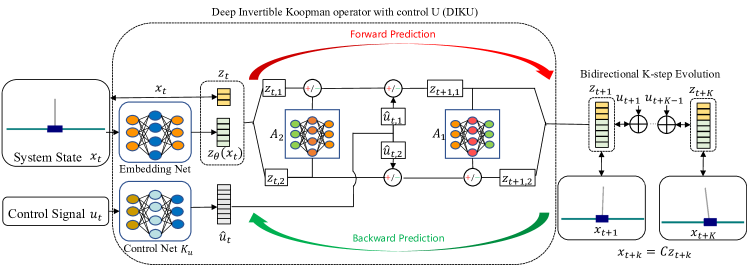
Figure 2: An overview of Deep Invertible Koopman operator with control U (DIKU) neural network model for long-horizon forward and backward dynamics prediction

We collect the training trajectory dataset as $\mathcal{D}=\left[X_{i}\in\mathbb{R}^{N\times n},U_{i}\in\mathbb{R}^{N\times m},i=1,\cdots,K\right]$. We define the following $K$-steps forward and backward dynamical loss as:

$$L(\theta_{z},\,\theta_{1},\theta_{2},\,\theta_{u}) =\frac{1-\gamma^{K}}{1-\gamma}\sum_{i=1}^{K}\gamma^{i-1}[MSE(X_{i},CZ_{i})$$ (11)

$$+MSE(X_{K-i+1},CZ_{K-i+1})]$$

where $MSE$ represents the mean square loss function and $\gamma$ denotes the weight decay constant. This $K$-steps loss is conductive to fine predictions in the long term.

III-B Online Approximate Time-Informed Set via Random Set and Koopman Operator Theories

Random set theory [15] guarantees asymptotic convergence to the convex hull of the reachable sets, whose relevant theorem is restated as follows:

Lemma III.1

[19] Let $\left\{(\bm{x}_{0}^{j},\bm{u}^{j})\right\}_{j=1}^{M}$ be i.i.d. sampled parameters in $\mathcal{X}_{0}\times\mathcal{U}^{k-1}$, where $M$ denotes the number of states. Define $\bm{x}_{t}^{j}$ as (1). Assume that the sampling distribution of the parameters satisfies $\mathbb{P}(\bm{x}_{t}^{j}\in G_{t})>0$ for any open set $G_{t}$ s.t. $\mathcal{X}_{t}\cap G_{t}\neq\emptyset$. Then, as $M\rightarrow\infty$, $\mathcal{X}_{t}$ converges to the convex hull of the RS $\text{Co}(\mathcal{X}_{t})$ almost surely.

A random set is defined as a map from a probability space to a family of sets. Consider sampling i.i.d. initial tuples $(\bm{x}_{0}^{j},\bm{u}_{0}^{j})\in\mathcal{X}^{f}_{0}\times\mathcal{U}$ and goal tuples $({\bm{x}}_{g}^{j},{\bm{u}}_{g}^{j})\in{\mathcal{X}}^{b}_{0}\times\mathcal{U}$ according to arbitrary probability distribution, where $j=1,\cdots,M$. Then, we encode the sampled states, obtaining the tuples in the lifted space, i.e., $(\bm{z}_{0}^{j},\bm{u}_{0}^{j})\in\mathcal{Z}^{f}_{0}\times\mathcal{U}$ and $({\bm{z}}_{g}^{j},{\bm{u}}_{g}^{j})\in{{{\mathcal{Z}}}}^{b}_{0}\times\mathcal{U}$. Next, we define a time step size $\delta$, and forecast the initial observables with the consistent $\bm{u}_{0}^{j}$ by (9) and backcast the goal observables with the ${\bm{u}}_{g}^{j}$ through (10) over $T$ time period simultaneously. We recover the predicted states from the generated observables. The convex hulls of the resulting states forward and backward propagation are denoted as $\text{Co}(\mathcal{X}^{f}_{0:T})$ and $\text{Co}({\mathcal{X}}^{b}_{-T:0})$, respectively.

In most cases, the convex polytopic sets $\mathcal{X}^{f}_{0}$ and ${\mathcal{X}}^{b}_{0}$ are mapped to nonconvex sets $\mathcal{Z}^{f}_{0}$ and ${{\mathcal{Z}}}^{b}_{0}$ since $\bm{z}(\bm{x})$ are nonlinear functions of $\bm{x}$. Our convex hulls will be over-approximations, sufficient for a heuristic sampling. To avoid returning a subset of the true and convex reachable set, we apply the adversarial sampling [19] to inflate the resulting convex hulls. To over-approximate FRS, after obtaining the set of the total $T$ period forward propagated trajectories $\mathcal{X}^{f}_{0:T}=\cup_{0\leq t\leq T}\{\bm{x}_{t}^{j}\}_{j=1}^{M}$, we use projected gradient ascent to maximize $\mathcal{L}^{M}(\bm{p})=\frac{1}{T}\sum_{t=\delta}^{T}\lVert\bm{x}_{t}(\bm{p}_{0})-\bm{c}_{t}^{M}\rVert^{2}_{Q_{t}^{M}}$ to regenerate initial tuples $\bm{p}_{0}=(\bm{x}_{0}^{j},\bm{u}_{0}^{j})$, where $Q_{t}^{M}$ are the positive definite matrices and $\bm{c}_{t}^{M}$ represent the geometric center of $\mathcal{X}^{f}_{t}$. $\bm{p}_{0}\leftarrow\bm{p}_{0}+\eta\nabla_{p}\mathcal{L}^{M}(\bm{x}_{\delta:T}^{j})$, where $\eta$ is a constant. After projecting the new $p_{0}$ onto $\mathcal{X}^{f}_{0}\times\mathcal{U}$, we propagate the new samples again using our DIKU and recover the trajectories to obtain $\{\bm{x}_{0:T}^{j}\}_{j=1}^{M}$ that inflates $\text{Co}(\mathcal{X}^{f}_{0:T})$. The propagated trajectories are updated as $\mathcal{X}^{f}_{0:T}\leftarrow\mathcal{X}^{f}_{0:T}\cup\{\bm{x}_{0:T}^{j}\}_{j=1}^{M}$. According to Lemma III.1, the over-approximation of FRS at time $t$ is $\mathcal{F}(0,t,\bm{x}_{0})=\text{Co}(\mathcal{X}^{f}_{t})$.

Similarly, we resample the goal tuples $p_{g}=(\bm{x}_{g}^{j},\bm{u}_{g}^{j})$ and backcast the $p_{g}$ by utilizing our backward DIKU and retrieve $\{{\bm{x}}_{-T:0}^{j}\}_{j=1}^{M}$. The adversarial sampling procedure of backward trajectories is ${\mathcal{X}}^{b}_{-T:0}\leftarrow{\mathcal{X}}^{b}_{-T:0}\cup\{{\bm{x}}_{-T:0}^{j}\}_{j=1}^{M}$. Given a terminal time instant $t_{f}$, the BRT over the time interval $[t,t_{f}]$ is over-approximated as $\mathcal{R}_{b}(t,t_{f},\mathcal{X}^{g})=\text{Co}({\mathcal{X}}^{b}_{t-t_{f}:0})$.

TIS is finally over-approximated with adequate number of samples $M$ as below according to (5)

$$\Omega(t_{f})=\!\!\!\mathop{\bigcup}\limits_{0\leq t\leq t_{f}}\!\!\!\text{Co}(\mathcal{X}^{f}_{t})\cap\text{Co}({\mathcal{X}}^{b}_{t-t_{f}:0}).$$ (12)

Although we can encode the states in the sets $\mathcal{X}^{f}_{0}$ and ${\mathcal{X}}^{b}_{0}$, it is intractable to embed the sets that have arbitrary shape representations into $\mathcal{Z}^{f}_{0}$ and ${{\mathcal{Z}}}^{b}_{0}$ [22]. Besides, inflation errors would be added in the process due to the extra $\bm{z}_{\theta_{z}}(\bm{x})$ even though we predefine the shapes of $\mathcal{Z}^{f}_{0}$ and ${{\mathcal{Z}}}^{b}_{t_{f}}$ based on experience. Thus, we only propagate the state but do not sample adversarially in the lifted space. System dynamics can be used directly with the sampling-based technique [19] to obtain a better accuracy while the forward DIKU, along with the technique, guarantees online FRS approximation, even possible for some unknown systems.

IV Online Time-Informed SKMP of Nonlinear Systems

Input: $(\bm{x}_{0},\mathcal{X}^{g});\;Q=\{\bm{x}_{0}\};\;E=\emptyset$

Output: $Tree(Q,E)$

1 $\tau=0;\;\mathcal{X}^{b}_{0}=\mathcal{X}^{g};\;M=1000;\;\eta;\;Tree(Q,E);$

2 while $\bm{x}_{0}\notin\rm{Co}(\mathcal{X}^{\textit{b}}_{\tau})$ do

3       $\tau=\tau-\delta$;

4$cost=-\tau$;

5 $\Omega(cost)=$ASKU$(cost,\bm{x}_{0},\mathcal{X}^{g},\eta,M)$; $\triangleright$ Sec. III-B

6 $cost^{\prime}=\infty$;

7 while $|(cost-cost^{\prime})/cost^{\prime}|>eps$ do

8       $cost^{\prime}=cost$; $[Tree,cost_{new}]=$TreeGrowth$(Tree,cost,\Omega(cost))$; if $cost_{new}\neq\infty$ then

9             $cost=cost_{new}$;

10             if $cost_{new}<cost$ then

11                   $\Omega(cost)=\Omega(cost^{\prime})\backslash(\text{Co}(\mathcal{X}^{f}_{cost^{\prime}})\cap\text{Co}({\mathcal{X}}^{b}_{0}))\backslash(\bigcup\limits_{0\leq t\leq cost+\delta}\text{Co}(\mathcal{X}^{f}_{t})\cap\text{Co}({\mathcal{X}}^{b}_{t-cost^{\prime}:t-cost-\delta}))$ ; $Tree=$Prune$(\Omega(cost),Tree,cost)$;

12            

13      else

14             $cost=cost+\delta_{2}$; $\Omega(cost)=\Omega(cost^{\prime})\cup(\text{Co}(\mathcal{X}^{f}_{cost})\cap\text{Co}({\mathcal{X}}^{b}_{0}))\cup(\bigcup\limits_{0\leq t\leq cost-\delta}\text{Co}(\mathcal{X}^{f}_{t})\cap\text{Co}({\mathcal{X}}^{b}_{t-cost:t-cost^{\prime}-\delta}))$ ;

15      

Algorithm 1 Online Time-Informed Sampling-based Kinodynamic Motion Planning

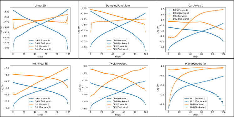
Figure 3: Comparison of forward and backward dynamics prediction by our DIKU and the DKU with consistency loss. The early predictions are more accurate than the late ones, which can be observed from the lines with plus markers of forward prediction from left to right and from those lines with dot markers of backward from right to left. The lower blue lines indicate smaller bidirectional dynamics evolution errors by DIKU, especially for nonlinear systems.

Algorithm $1$ outlines the procedure of our planning method. We obtain the optimal time cost ignoring obstacles by determining the index of BRS that contains the start state $\bm{x}_{0}$. The TIS corresponding to this $cost$ is constructed using our ASKU approach in Section III-B. Then, we grow a search tree within $\Omega(cost)$ and compute the tree’s time cost $cost_{new}$ while considering obstacles. $\Omega(cost)$ reduces and we eliminate the nodes outside it once we find a better suboptimal solution. In contrast, we extend the optimal time of the planning problem $\delta_{2}$s and expand the TIS since a collision-free solution less than $cost$ might not exist.

Algorithm $2$ describes the procedure to grow a search tree with a direct sampling technique, HNR sampling method [23], within the components of TIS. A time $t$ is first uniformly sampled in $[0,cost]$ as the cost-to-come of the sample to be generated. If a random number is generated below the threshold $\mu$, we draw a sample within the TIS to accelerate the convergence speed; otherwise, within the entire state space. We compute the longest time cost from $t$ to reach the goal. A linear programming problem, subject to the linear inequalities of the FRS at $t$ and BRS at $t^{\prime}$, is formulated to check if there exists any intersection. We decrease the cost-to-go until finding the minimum value. A valid cost-to-go $\bar{t}$ is then uniformly sampled. Finally, we use the vertex inclusion algorithm [13] and an off-the-shelf SKMP to find a solution tree and return its cost $cost_{new}$, if there exists.

V Simulation Experiments

In this section, we conduct simulation experiments to 1) verify our DIKU’s bidirectional long-term prediction performance, 2) demonstrate the high performance of our ASKU’s reachability analysis for TIS, and 3) show the improved planning efficiency of our online time-informed SKMP.

Input: $Tree,cost,\Omega(cost)$

Output: $Tree,cost_{new}$

1 for $i=1:N$ do

2       $t=\text{UniformSample}([0,cost])$; $\triangleright$ cost-to-come

3       if $\rm{Rand}(0,1)<\mu$ then

4             $t^{\prime}=t-cost$; $\triangleright$ the maximum cost-to-go while $\{\bm{x}\!\in\!\mathcal{X}|\rm{Co}(\mathcal{X}^{\textit{f}}_{\textit{t}})\!\cap\!\rm{Co}(\mathcal{X}^{\textit{b}}_{\textit{t}^{\prime}}),\textit{t}^{\prime}\!\leq\!0\}\!\neq\!\emptyset$ do

5                   $t^{\prime}=t^{\prime}+\delta$; $\triangleright$ find the minimum cost-to-go

6            $\bar{t}=\text{UniformSample}([t-cost,t^{\prime}))$; $\bm{x}_{new}=$HNR$(\{\bm{x}\in\mathcal{X}\,|\,\text{Co}(\mathcal{X}^{f}_{t})\cap\text{Co}(\mathcal{X}^{b}_{\bar{t}})\})$;

7      else

8             $\bm{x}_{new}=$Sample$(\mathcal{X})$;

9      $[Tree,cost_{new}]=\text{SKMP}(Tree,\bm{x}_{new},t)$;

10if $\bf{no}$ node $\in\mathcal{X}^{g}$ then

11       $cost_{new}=\infty$;

Algorithm 2 Tree Growth

V-A Experiment Environments

We have six dynamic systems for evaluation, including a (a) 2D linear system in [14] (2D-L), (b) 3D polynomial nonlinear system in [14] (3D-PNL), (c) CartPole in [16], (d) DampingPendulum in [16], (e) two-link robot in [16], and (f) planar quadrotor in [24]. For each system, a total of 10000, 2500, and 5000 trajectories are generated by simulating the dynamics, designated for training, validation, and testing, respectively. Our experiments were conducted in Python and C++ using a 64-bit workstation with an Intel Core i9-13900K processor, NVIDIA 4090 GPU, and 128GB RAM, running Ubuntu 20.04 OS.

V-B Long-Term Forward and Backward Dynamics Prediction

We evaluate the long horizon forward and backward dynamical prediction performance of our DIKU model on the six dynamics and compare them with the existing method. We extend the Deep KoopmanU with Control (DKU) in [16] to compute the backward counterpart of (8) through additionally training an independent linear NN of $K_{x}^{-1}$. We impose the weights of parameterized $K_{x}$ and $K_{x}^{-1}$ in a consistency loss as in [25]. One INN module is constructed, where $\bm{z}_{t,2}$ is randomly selected. The hidden layers of $A_{1}$ and $A_{2}$ are $[128,64,32]$ with the ReLU [26] in the dynamics (a)-(e), while with linear activation functions in (f). The structures and weights of embedding and control nets, training and testing datasets, learning rate $0.001$, batch size $1024$, Adam optimizer [27], and K step loss with $\gamma=0.9$ of the extended DKU and DIKU are identical for each system.

The 100-step bidirectional prediction results are shown in Fig. 3. We calculate the mean of the log10 of the maximum error. It can be seen that our DIKU (blue) can bidirectionally predict much more accurate states in the long horizon than the DKU (yellow). Unlike the DKU which uses different structures, parameters, and a soft loss function to train $K_{x}$ and $K_{x}^{-1}$ for bidirectional prediction, our model allows direct back prediction through the INN structure (10), benefiting a better inference and convergence in training. Another reason is that the control field’s nonlinearity can be reflected by the INN’s translation functions. Consequently, DIKU paves the way to efficiently perform accurate long-term bidirectional propagation in sampling-based reachability analysis.

V-C Online Time-Informed Set Approximation

We compare our basic sampling-based approach (ours) and its over-approximation version, the ASKU, (ours(AS)) with level set method [28] (ground truth), ellipsoidal toolbox [29] (ET), and relaxed HJB equation method [14] (RHJB) for the dynamics (a). Set identical time step $0.05$s and horizon $T=5$s. We evaluate the volume convergence of ours for computing BRT and show the results in Fig. 5. We set $M=1000$, $\eta=0.015$, and $\eta=0.04$ for forward and backward prediction to let the gradient and $\bm{p}_{0}$ have the same order of magnitude. We use the ellipsoidal parameters of initial and goal sets and control limits in [14]. The reachable sets and tubes that constitute TIS are shown in Fig. LABEL:fig:tis. Since the ground truth has to discretize the spaces to calculate the numerical result of the HJB partial differential equation, we have tried to reduce the number of girds to save time while guaranteeing the quality of the reachable sets. Table I records the computation costs of reachable tubes. The ground truth takes plenty of time to return a fine FRT. ET must be calculated in 30 random directions, resulting in a heavy computation burden and a more compact ellipsoid than RHJB. RHJB predefines the centers of the external ellipsoids instead of treating them as decision variables since that makes solving SOS optimization intractable. However, the centers highly influence the convergence of RHJB, leading to no solution sometimes. Although sometimes feasible for the system, it is time-consuming and may cause drift, as seen in the purple BRT in Fig. LABEL:fig:tis. These methods also suffer from the curse of dimensionality. In contrast, ours and ASKU can be completed in near real-time. Note that ASKU can be applied to linear and nonlinear systems that can be learned regardless of the number of dimensions, thanks to DIKU’s NN bidirectional propagation. Facing the true convex reachable set, our ASKU can still return over-approximation online.

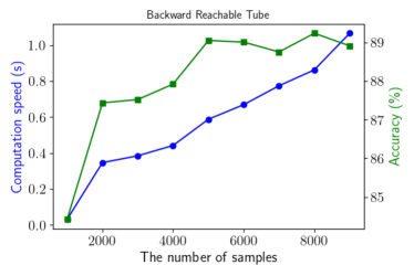
Figure 5: Volume convergence (green line) and speed (blue line) on DIKU with a varying number of samples $M$ for our basic BRT approximation. The volume accuracy is computed by being divided by the volume of ground truth. A high degree of accuracy can be obtained at the cost of computation speed.

V-D Online Time-Informed Kinodynamic Motion Planning

TABLE I: Computation times [s] of the Forward/Backward reachable tubes for the example 2D system in [14]

	Level Set [28]	ET [29]	RHJB [14]	Ours	Ours (AS)
FRT	47.46	51.13	22.17	0.03	0.16
BRT	5.71	6.07	23.31	0.03	0.16

We conduct the problem (2) on all dynamics between SST [8] and our algorithm while only comparing the approach in [14] with default parameters on (a) and (b). We set $\delta_{2}=0.5$s, and $M=1000$ and valid $\eta$ for our method. Set $\mu=0.9$ to accelerate our search progress and $N=500$ in [14] and ours. A library of TIS computed offline exists only for [14]. The running time of approximating TIS is not counted in [14] but it is included in ours because ours is an online time-informed method. The computation time is measured as the condition (line 7, Alg. 1) is no longer satisfied.

TABLE II: Comparison results of the running time, path qualities, and the number of nodes for benchmarks and ours

		$T_{IN}[s]$	$C_{IN}[s]$	$T_{OP}[s]$	$C_{OP}[s]$	$N_{node}(\times 10^{2})$
2D-L	Ours	$\bm{0.87}$	$\bm{4.68\!\!\pm\!\!0.10}$	$\bm{6.87}$	$\bm{4.44\!\!\pm\!\!0.09}$	$\bm{3.21\!\!\pm\!\!0.7}$
	[14]	$1.02$	$4.78\!\!\pm\!\!0.12$	$7.02$	$4.46\!\!\pm\!\!0.12$	$3.4\!\!\pm\!\!0.81$
	SST	$1.78$	$9.11\!\!\pm\!\!2.91$	$25.78$	$4.87\!\!\pm\!\!0.60$	$12.9\!\!\pm\!\!0.29$
3D-PNL	Ours	$\bm{1.45}$	$\bm{4.22\!\!\pm\!\!0.21}$	$\bm{4.45}$	$\bm{4.07\!\!\pm\!\!0.08}$	$\bm{1.67\!\!\pm\!\!0.27}$
	[14]	$1.68$	$4.31\!\!\pm\!\!0.22$	$4.68$	$4.08\!\!\pm\!\!0.10$	$1.71\!\!\pm\!\!0.28$
	SST	$26.37$	$6.38\!\!\pm\!\!2.08$	$56.37$	$5.33\!\!\pm\!\!1.40$	$28.51\!\!\pm\!\!7.58$
CartPole	Ours	$\bm{5.26}$	$\bm{4.91\!\!\pm\!\!1.74}$	$\bm{11.26}$	$\bm{4.18\!\!\pm\!\!1.73}$	$\bm{5.87\!\!\pm\!\!1.91}$
	SST	$14.69$	$8.21\!\!\pm\!\!4.90$	$29.69$	$6.15\!\!\pm\!\!4.21$	$19.44\!\!\pm\!\!5.59$
Damping	Ours	$\bm{6.23}$	$\bm{2.08\!\!\pm\!\!0.35}$	$\bm{10.57}$	$\bm{1.85\!\!\pm\!\!0.39}$	$\bm{5.26\!\!\pm\!\!1.78}$
Pendulum	SST	$21.2$	$2.38\!\!\pm\!\!1.31$	$33.2$	$1.91\!\!\pm\!\!0.96$	$21.25\!\!\pm\!\!6.51$
Two-link	Ours	$\bm{8.34}$	$\bm{4.72\!\!\pm\!\!1.17}$	$\bm{17.34}$	$\bm{4.39\!\!\pm\!\!1.56}$	$\bm{6.52\!\!\pm\!\!2.03}$
Robot	SST	$27.12$	$7.10\!\!\pm\!\!5.20$	$45.12$	$4.60\!\!\pm\!\!4.60$	$26.35\!\!\pm\!\!12.75$
Planar	Ours	$\bm{15.64}$	$\bm{8.50\!\!\pm\!\!1.02}$	$\bm{24.64}$	$\bm{7.72\!\!\pm\!\!1.12}$	$\bm{45.54\!\!\pm\!\!13.04}$
Quadrotor	SST	$39.91$	$10.52\!\!\pm\!\!2.83$	$57.91$	$8.90\!\!\pm\!\!2.62$	$234.03\!\!\pm\!\!52.21$

Fig. LABEL:fig:problem depicts the schematics of the planning problems and Table II reports the statistical results of 100 trials. $T_{IN}$ and $T_{OP}$ represent the computation time of discovering the initial solution and final suboptimal solution, respectively. $C_{IN}$ and $C_{OP}$ stand for the solutions’ costs, respectively. $N_{node}$ denotes the total number of nodes at the conclusion. Since our method attempts to grow the search tree within $\Omega$ from the beginning, better initial and final collision-free solutions are returned much faster than SST in all environments. It can be observed that our algorithm finds better initial and final solutions more quickly compared with [14] because we directly draw samples in a tighter TIS. It can also apply to the nonlinear systems (c)-(f) other than the PNL system (b). The sampling acceptance rate among the six systems is $82\%$ on average. In terms of memory burdens, our algorithm and [14] require fewer nodes than SST in the environments of (a) and (b) due to the elimination effect of the Prune() function. In the other environments, our method retains the tree with $19.5\%\sim 30.2\%$ nodes since we sample within the $\Omega(cost)$ that contains the optimal solution.

VI CONCLUSION

In this work, we realize online TIS approximation and propose an online time-informed SKMP of nonlinear systems. Our proposed Deep Invertible Koopman operator with control U (DIKU) model accurately infers forward and backward dynamics propagation over a long horizon by designing the INN-based auxiliary network. The developed ASKU method can over-approximate TIS in convex sets for a variety of systems at little cost through conducting adversarial sampling for DIKU bidirectional propagation. The time-optimal SKMP that directly samples in the TIS takes less planning time than the [14] algorithm although counting the TIS computation costs. Our next research direction is to improve our DIKU and realize bidirectional search tree growth.

References

- [1] Steven M LaValle and James J Kuffner Jr. Randomized kinodynamic planning. The international journal of robotics research, 20(5):378–400, 2001.
- [2] Sertac Karaman and Emilio Frazzoli. Sampling-based algorithms for optimal motion planning. The international journal of robotics research, 30(7):846–894, 2011.
- [3] Fei Meng, Liangliang Chen, Han Ma, Jiankun Wang, and Max Q-H Meng. Nr-rrt: Neural risk-aware near-optimal path planning in uncertain nonconvex environments. IEEE Transactions on Automation Science and Engineering, 2022.
- [4] Fei Meng, Liangliang Chen, Han Ma, Jiankun Wang, and Max Q-H Meng. Learning-based risk-bounded path planning under environmental uncertainty. IEEE Transactions on Automation Science and Engineering, 2023.
- [5] Jonathan D Gammell, Siddhartha S Srinivasa, and Timothy D Barfoot. Informed rrt: Optimal sampling-based path planning focused via direct sampling of an admissible ellipsoidal heuristic. In 2014 IEEE/RSJ international conference on intelligent robots and systems, pages 2997–3004. IEEE, 2014.
- [6] Alejandro Perez, Robert Platt, George Konidaris, Leslie Kaelbling, and Tomas Lozano-Perez. Lqr-rrt*: Optimal sampling-based motion planning with automatically derived extension heuristics. In 2012 IEEE International Conference on Robotics and Automation, pages 2537–2542. IEEE, 2012.
- [7] Dustin J. Webb and Jur van den Berg. Kinodynamic rrt*: Asymptotically optimal motion planning for robots with linear dynamics. In 2013 IEEE International Conference on Robotics and Automation, pages 5054–5061, 2013.
- [8] Yanbo Li, Zakary Littlefield, and Kostas E Bekris. Asymptotically optimal sampling-based kinodynamic planning. The International Journal of Robotics Research, 35(5):528–564, 2016.
- [9] Tobias Kunz, Andrea Thomaz, and Henrik Christensen. Hierarchical rejection sampling for informed kinodynamic planning in high-dimensional spaces. In 2016 IEEE International Conference on Robotics and Automation (ICRA), pages 89–96. IEEE, 2016.
- [10] Daqing Yi, Rohan Thakker, Cole Gulino, Oren Salzman, and Siddhartha Srinivasa. Generalizing informed sampling for asymptotically-optimal sampling-based kinodynamic planning via markov chain monte carlo. In 2018 IEEE International Conference on Robotics and Automation (ICRA), pages 7063–7070. IEEE, 2018.
- [11] Alexander Shkolnik, Matthew Walter, and Russ Tedrake. Reachability-guided sampling for planning under differential constraints. In 2009 IEEE International Conference on Robotics and Automation, pages 2859–2865. IEEE, 2009.
- [12] Albert Wu, Sadra Sadraddini, and Russ Tedrake. R3t: Rapidly-exploring random reachable set tree for optimal kinodynamic planning of nonlinear hybrid systems. In 2020 IEEE International Conference on Robotics and Automation (ICRA), pages 4245–4251. IEEE, 2020.
- [13] Sagar Suhas Joshi, Seth Hutchinson, and Panagiotis Tsiotras. Tie: Time-informed exploration for robot motion planning. IEEE Robotics and Automation Letters, 6(2):3585–3591, 2021.
- [14] Yongxing Tang, Zhanxia Zhu, and Hongwen Zhang. A reachability-based spatio-temporal sampling strategy for kinodynamic motion planning. IEEE Robotics and Automation Letters, 8(1):448–455, 2022.
- [15] Ilya S Molchanov and Ilya S Molchanov. Theory of random sets, volume 19. Springer, 2005.
- [16] Haojie Shi and Max Q-H Meng. Deep koopman operator with control for nonlinear systems. IEEE Robotics and Automation Letters, 7(3):7700–7707, 2022.
- [17] Somil Bansal and Claire J Tomlin. Deepreach: A deep learning approach to high-dimensional reachability. In 2021 IEEE International Conference on Robotics and Automation (ICRA), pages 1817–1824. IEEE, 2021.
- [18] Laurent Dinh, Jascha Sohl-Dickstein, and Samy Bengio. Density estimation using real nvp. arXiv preprint arXiv:1605.08803, 2016.
- [19] Thomas Lew and Marco Pavone. Sampling-based reachability analysis: A random set theory approach with adversarial sampling. In Conference on robot learning, pages 2055–2070. PMLR, 2021.
- [20] Kshitij Tayal, Arvind Renganathan, Rahul Ghosh, Xiaowei Jia, and Vipin Kumar. Koopman invertible autoencoder: Leveraging forward and backward dynamics for temporal modeling. arXiv preprint arXiv:2309.10291, 2023.
- [21] Milan Korda and Igor Mezić. Linear predictors for nonlinear dynamical systems: Koopman operator meets model predictive control. Automatica, 93:149–160, 2018.
- [22] Stanley Bak, Sergiy Bogomolov, Parasara Sridhar Duggirala, Adam R Gerlach, and Kostiantyn Potomkin. Reachability of black-box nonlinear systems after koopman operator linearization. IFAC-PapersOnLine, 54(5):253–258, 2021.
- [23] Seksan Kiatsupaibul, Robert L. Smith, and Zelda B. Zabinsky. An analysis of a variation of hit-and-run for uniform sampling from general regions. 21(3), feb 2011.
- [24] Carl Folkestad and Joel W Burdick. Koopman nmpc: Koopman-based learning and nonlinear model predictive control of control-affine systems. In 2021 IEEE International Conference on Robotics and Automation (ICRA), pages 7350–7356. IEEE, 2021.
- [25] Omri Azencot, N Benjamin Erichson, Vanessa Lin, and Michael Mahoney. Forecasting sequential data using consistent koopman autoencoders. In International Conference on Machine Learning, pages 475–485. PMLR, 2020.
- [26] Abien Fred Agarap. Deep learning using rectified linear units (relu). arXiv preprint arXiv:1803.08375, 2018.
- [27] Diederik P Kingma and Jimmy Ba. Adam: A method for stochastic optimization. arXiv preprint arXiv:1412.6980, 2014.
- [28] Ian M Mitchell, Alexandre M Bayen, and Claire J Tomlin. A time-dependent hamilton-jacobi formulation of reachable sets for continuous dynamic games. IEEE Transactions on automatic control, 50(7):947–957, 2005.
- [29] Alexander B Kurzhanski and Pravin Varaiya. Ellipsoidal techniques for reachability analysis. In International workshop on hybrid systems: Computation and control, pages 202–214. Springer, 2000.