Timely Requesting for Time-Critical Content Users in Decentralized F-RANs

Abstract

With the rising demand for high-rate and timely communications, fog radio access networks (F-RANs) offer a promising solution. This work investigates age of information (AoI) performance in F-RANs, consisting of multiple content users (CUs), enhanced remote radio heads (eRRHs), and content providers (CPs). Time-critical CUs need rapid content updates from CPs but cannot communicate directly with them; instead, eRRHs act as intermediaries. CUs decide whether to request content from a CP and which eRRH to send the request to, while eRRHs decide whether to command CPs to update content or use cached content. We study two general classes of policies: (i) oblivious policies, where decision-making is independent of historical information, and (ii) non-oblivious policies, where decisions are influenced by historical information. First, we obtain closed-form expressions for the average AoI of eRRHs under both policy types. Due to the complexity of calculating closed-form expressions for CUs, we then derive general upper bounds for their average AoI. Next, we identify optimal policies for both types. Under both optimal policies, each CU requests content from each CP at an equal rate, consolidating all requests to a single eRRH when demand is low or resources are limited, and distributing requests evenly among eRRHs when demand is high and resources are ample. eRRHs command content from each CP at an equal rate under an optimal oblivious policy, while prioritize the CP with the highest age under an optimal non-oblivious policy. Our numerical results validate these theoretical findings.

Index Terms—Age of information, multi-hop networks, fog radio access networks, decentralized policies, stationary randomized policies.

I Introduction

With the proliferation of multimedia services, a massive numbers of end-users are generating large volumes of data-intensive and time-sensitive applications in wireless networks. This has led to a surge in the demand for high-rate and timely communications. Recently, fog radio access networks (F-RANs) have emerged as a promising solution to meet this growing demand. Fog computing, a new paradigm, provides a platform for local computing, distribution, and storage on end-user devices, as opposed to relying solely on centralized data centers [1]. As an evolution of cloud radio access networks (C-RANs) [2], F-RANs feature fog access points to a centralized baseband signal processing unit via fronthaul links. There fog access points are equipped with caching capabilities to proactively store content [3]. This approach allows end-users to access data locally without needing to reach the baseband unit (BBU) pool, thus reducing the load on both the fronthaul links and the BBU pool.

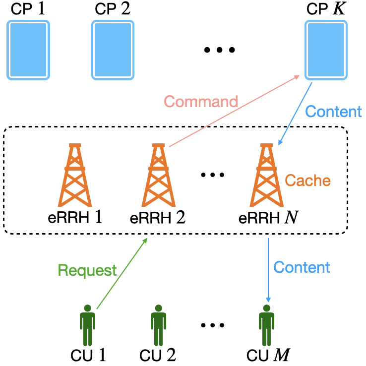
Figure 1: An example of a decentralized F-RAN.

This paper addresses the issue of timely content requests for time-critical end-users, also known as content users (CUs), in decentralized F-RANs (see Fig. 1). In an F-RAN, multiple content providers (CPs), enhanced remote radio heads (eRRHs), and CUs interact in a network. CUs, which require timely content from CPs, cannot communicate directly with CPs. Instead, eRRHs act as gateways. Upon receiving requests from CUs, eRRHs can either command CPs to provide new content or retrieve cached content [4]. Given that all CUs are time-critical, the objective is to optimize the information freshness for CUs by proposing optimal policies for both CUs and eRRHs. To capture freshness, we use the Age of Information (AoI) metric [5], which measures the freshness of information at the receiver side. This metric is crucial in Internet of Things (IoT) applications where the timeliness of information is essential, such as in system status monitoring [5]. Addressing this problem involves two main sequential steps: (i) CUs making request decisions based on demand and resource availability, and (ii) eRRHs making command decisions based on available resources. The practical impact of this work is significant, as optimizing AoI in F-RANs can enhance the efficiency and responsiveness of various real-time applications. These include smart cities, autonomous vehicles, industrial automation, and health monitoring systems [6, 7, 8], where timely and reliable information delivery is critical. Improved AoI management ensures that these systems operate with up-to-date information, reducing latency and enhancing overall performance and reliability.

Associated with this problem are the following primary challenges.

• (i) Decentralization among CUs and eRRHs: In a decentralized F-RAN, each CU and eRRH makes decisions based solely on their local information. This independence in decision-making complicates coordination among CUs and eRRHs.

• (ii) Inter-dependence within each CU: During one time slot, a CU can send at most one request per CP to eRRHs, creating inter-dependence in the decisions made by each CU. This inter-dependence makes analysis extremely difficult, and the age of version metric introduced in previous works [9, 10, 8, 11, 12] cannot be applied.

• (iii) Complexity from the network topology: An F-RAN operates as a two-hop network with multiple receiver nodes at each hop. Designing an optimal policy for F-RANs is challenging due to the limited communication resources.

• (iv) Historical information: Since CUs require the freshest content, any outdated content in the eRRHs’ local cache must be discarded. This requirement makes the objective function a combination of multiple min functions, adding to the complexity of the analysis.

By addressing these challenges, our objective becomes clearer: to develop and analyze an optimal decentralized strategy that effectively utilizes historical information to optimize freshness for time-critical CUs in F-RANs.

I-A Related Work

The AoI has been proposed as ametric to quantify the freshness of information at the receiver side [5]. By definition, AoI measures the time elapsed since the generation of the most recent information available at the receiver side. Formally, AoI is a function of both the frequency of packet transmissions and the delay experienced by packets in the communication network [6]. This work intersects three primary areas: (i) AoI in multi-hop networks, (ii) AoI in edge/fog computing networks, and (iii) AoI in cache updating systems. These areas overlap to some extent. Below, we describe the related work in these fields.

I-A1 AoI in Multi-hop Networks

There exists a significant body of research focusing on the analysis of AoI in single-hop networks. However, studies on AoI in multi-hop networks are less prevalent due to the complexities arising from network topologies and interferences among nodes.

One of the earliest works addressing AoI optimization in general networks is [13]. This study considered multi-source multi-hop wireless networks where nodes function as both senders and receivers. It derived lower and upper bounds on average and peak AoI and proposed an optimal scheduling policy to minimize these metrics. However, the framework is limited to connected networks with nine or fewer nodes. In contrast, [14] proposed near-optimal periodic status update scheduling policies using graph properties and obtained lower bounds for average and peak AoI. These policies can be applied to any connected topology. Another early work, [15], investigated the minimization of AoI for a single information flow in interference-free multi-hop networks. It proved that a preemptive last-generated, first-served policy results in smaller age processes across all nodes in the network compared to any other causal policy (in a stochastic ordering sense) if the packet transmission times are exponentially distributed.

Subsequent studies have explored optimal policies in general multi-hop networks. [16] proposed a near-optimal network control policy, achieving an average AoI close to a theoretical lower bound. [17, 18] investigated optimal stationary randomized policies and optimal scheduling policies, termed age difference policies and age debt policies. The optimal age debt policy can be applied to general multi-hop networks with unicast, multicast, and broadcast flows. Additionally, [19] explored the trade-off between AoI and throughput in general multi-hop wireless networks, identifying Pareto-optimal points and providing insights into balancing AoI and throughput. [20] examined AoI optimization using OFDM for multi-channel spectrum access, focusing on the impacts of real-world factors such as orthogonal channel access and wireless interference on AoI. [21] investigated AoI in multi-hop multicast cache-enabled networks with inter-update times that are not necessarily exponentially distributed. The study demonstrated that the expected AoI has an additive structure and is directly proportional to the variance of inter-update times across all links. Finally, [22] proposed decentralized policies to minimize AoI and estimation error, emphasizing scalability. These policies can be applied to networks of any size, offering a flexible solution for large-scale implementations.

I-A2 AoI in Edge/Fog Computing Networks

In mobile edge computing (MEC) and fog computing networks, information messages typically go through two phases: the transmission phase and the computing/processing phase. Consequently, mathematical models for these networks are often established as two-hop networks and tandem queues.

The first study to focus on the AoI for edge computing applications is [23], which primarily calculated the average AoI. [24] investigated the average AoI in a network with multiple sensors and one destination. The study derived analytical expressions for the average peak AoI for different sensors and designed a derivative-free algorithm to obtain the optimal updating frequency. A generic tandem model with a first-come-first-serve discipline was considered in [25]. The authors obtained the distribution of peak AoI for both M/M/1-M/D/1 and M/M/1-M/M/1 tandems. Building on this, [26] took a step further by considering both average and peak AoI in general tandems with packet management. This work illustrated the tradeoff between computation and transmission when optimizing AoI. In [27], both local computing and edge computing schemes under a first-come-first-serve discipline were considered in an MEC system with multiple users and a single base station (BS). The average AoI of these two computing schemes was derived.

[28] and [29] investigated information freshness in MEC networks from a multi-access perspective. [28] considered multi-access edge computing where a BS serves traffic streams from multiple IoT devices. Packets from each stream arrive at the base station and are then forwarded to their respective destinations after processing by the MEC node. An optimal scheduling algorithm to minimize average AoI was proposed using integer linear programming. [29] considered a NOMA-based MEC offloading scenario where multiple devices use NOMA to offload their computing tasks to an AP integrated with an MEC server. Leveraging tools from queuing theory, the authors proposed an iterative algorithm to obtain the closed-form solution for AoI.

[30] and [31] explored the average AoI in MEC networks using other mathematical tools. [30] considered MEC-enabled IoT networks with multiple source-destination pairs and heterogeneous edge servers. Using game-theoretical analysis, an age-optimal computation-intensive update scheduling strategy was proposed based on Nash equilibrium. Reinforcement learning is also a powerful tool in this context. [31] proposed a computation offloading method based on a directed acyclic graph task model, which models task dependencies. The algorithm combined the advantages of deep Q-network, double deep Q-network, and dueling deep Q-network algorithms to optimize AoI.

I-A3 AoI in Cache Updating Systems

In cache updating systems, it is crucial to ensure that cached data remains current to prevent serving outdated information to users, which could lead to incorrect decisions. In [32], a system is examined where a local cache maintains multiple content items. The authors introduced a popularity-weighted AoI metric for updating dynamic content in a local cache, demonstrating that the optimal policy involves updating the items in the cache at a rate proportional to the square root of their popularity.

Several studies, including [9, 10, 11, 12, 8], introduced a new metric called the age of version to measure information freshness in cache updating systems. In [9], a caching scenario for dynamically changing content was considered, and the authors showed that the optimal caching strategy allocates cache space based solely on item popularity. In [10], three types of cache updating systems were explored: (i) one source, one cache, and one user; (ii) one source, a sequence of cascading caches, and one user; and (iii) one user, one cache, and multiple sources. In these systems, the optimal rate allocation policies for the caches and users are threshold policies. [8] studied timely cache updating policies in parallel multi-relay networks, deriving an upper bound on the average AoI for users and proposing a sub-optimal policy using a stochastic hybrid system approach. [11] investigated the optimal scheduling of cache updates while accounting for content recommendation and AoI. Although the problem was proven NP-hard, efficient algorithms were proposed for the sub-optimization problem. The framework was extended in [12] to a cache updating system with randomly located caches following a Poisson point process, where the distribution of user-perceived version age of files was derived.

AoI for energy-harvesting sensors is another important research direction in cache updating systems. The average AoI for an energy-harvesting sensor with caching capability was studied in [33], where a probabilistic model was used to determine decisions, and the closed form was derived. A request-based scenario was considered in [34], where a cache-enabled base station stores the most recent status observed by energy-harvesting sensors and delivers the cached status to applications upon request. The proposed optimal scheduling policy achieved a 16% performance gain compared to the traditional greedy policy.

The work most closely related to ours is [8], which investigated timely cache updating policies in parallel multi-relay networks. Although the network topologies in both works are similar, there are key differences: (i) Applications: [8] addressed cache updating systems for $N$ files in a time-continuous setting, while our work focused on decentralized F-RANs in a time-discrete setting. (ii) Number of senders: [8] involved only one sender, whereas our work included multiple senders, making our scenario more general since the decisions of one sender affect others. (iii) Decisions within senders: In [8], decisions within the sender are independent, whereas in our work, decisions are inter-dependent, significantly increasing the analysis complexity and making our scenario more general. Our theoretical results encompass those of [8] (see the discussions below Lemma 1). (iv) Policies: [8] used oblivious policies, where decisions are independent of historical information. In contrast, our work includes both oblivious and non-oblivious policies, with the latter depending on historical information. Therefore, our work investigated a more general case and achieved more comprehensive results.

I-B Contributions

In this paper, we address the issue of optimizing the information freshness for time-critical CUs in F-RANs. In each time slot, every CU independently makes decisions based on its own information, focusing on two key aspects: (i) determining whether to send a request to eRRHs for each CP, and (ii) selecting an eRRH to receive the request for each CP. Upon receiving requests, eRRHs decide whether to command CPs to send new content or to retrieve content from their local cache. Our goal is to minimize the average AoI for CUs by proposing decentralized stationary randomized policies. We explore two classes of strategies: (i) oblivious policies, where decisions are made independently of historical information, and (ii) non-oblivious policies, where decisions are influenced by historical information [7, 22]. We begin by focusing on a F-RAN with $2$ CUs, $2$ eRRHs, and $2$ CPs (see Section III and Section IV). From this initial setup, we then extend our framework and theoretical results to general networks with arbitrary number of CUs, eRRHs, and CPs (see Appendix I).

In an F-RAN, CUs receive content from CPs via eRRHs, making the AoI of CUs dependent on the AoI of eRRHs. To understand this relationship, we establish recursive formulas for the AoI of both CUs and eRRHs and examine their average AoI. Under oblivious policies, where decisions are made without historical context, the AoI of an eRRH (associated with a CP) follows a geometric distribution. We derive closed-form expressions for the average AoI of eRRHs in this scenario (see Theorem 1). For non-oblivious policies, where eRRHs utilize historical information, the analysis is more complex. To address this, we introduce an ergodic two-dimensional Markov chain to derive closed-form expressions for the average AoI (see Theorem 4).

Deriving the closed-form expressions for the average AoI of CUs is challenging due to the discarding of outdated content from eRRHs by the CUs. This introduces a set of min functions into the AoI calculations for CUs. As a result, we derive two upper bounds for the average AoI of CUs: see Theorem 2 for oblivious cases and Theorem 5 for non-oblivious cases. The first upper bound represents the average AoI in an extreme scenario where eRRHs only send new packets and do not transmit previously cached ones. This bound is more accurate when the rates of sending requests to different eRRHs for a CP differ significantly. The second upper bound reflects the average AoI in an extreme case where CUs replace the most recently received packets with the currently delivered packets from eRRHs, even if they are older. This bound is more accurate when the rates of sending requests to different eRRHs for a CP are close to each other.

Even without the closed-form expressions for AoI, we theoretically determine the optimal policies in both oblivious and non-oblivious scenarios. An optimal oblivious policy features the following (see Theorem 3): (i) Each eRRH commands content from each CP at an equal rate. (ii) Each CU sends requests to eRRHs for each CP at an equal rate. (iii) To request content from a CP, each CU consolidates all rates to single eRRH when the demand is low or communication resources are limited, while requests are distributed evenly among eRRHs when the demand is high and communication resources are ample. An optimal non-oblivious policy shares similar features with the optimal oblivious one, except for the first feature (see Theorem 6). In non-oblivious policies, each eRRH consolidates all rates to the CP with the highest age in a time slot. This is because the rates of commands vary with the current ages of the CPs, so the best utilization of rates is to allocate them entirely to the CP with the highest age. Our numerical results verify these theoretical findings.

The paper is organized as follows. In Section II, we introduce the system model. In Section III and Section IV, we theoretically obtain an optimal strategy in oblivious and non-oblivious cases, respectively. Simulation results are presented in Section V and our derivations are verified numerically. Finally, we conclude in Section VI.

II System Model

We consider a F-RAN consisting of $M$ CUs, $N$ eRRHs, and $K$ CPs. CUs, eRRHs and CPs are satistically identical within their respective groups. We denote the sets of CUs, eRRHs, and CPs as $[M]=\{1,2,\cdots,M\}$, $[N]=\{1,2,\cdots,N\}$, and $[K]=\{1,2,\cdots,K\}$, respectively. An example of a F-RAN is depicted in Fig. 2. CUs require time-critial content from CPs but cannot communicate with them directly. Instead, eRRHs in the network act as gateways [4]. Content from CPs is transmitted through packets; therefore, we use the terms content and packets interchangeably. These eRRHs have the capability to cache and transmit packets. If CU $m$ needs the latest time-critical packet from CP $k$, it sends a request to eRRHs. The eRRH that receives the request is denoted as eRRH $n$. After receiving the request, eRRH $n$ can either retrieve a cached packet locally or command CP $k$ to update a new packet to serve the request. In this network, all CUs are time-sensitive and require packet updates as quickly as possible.

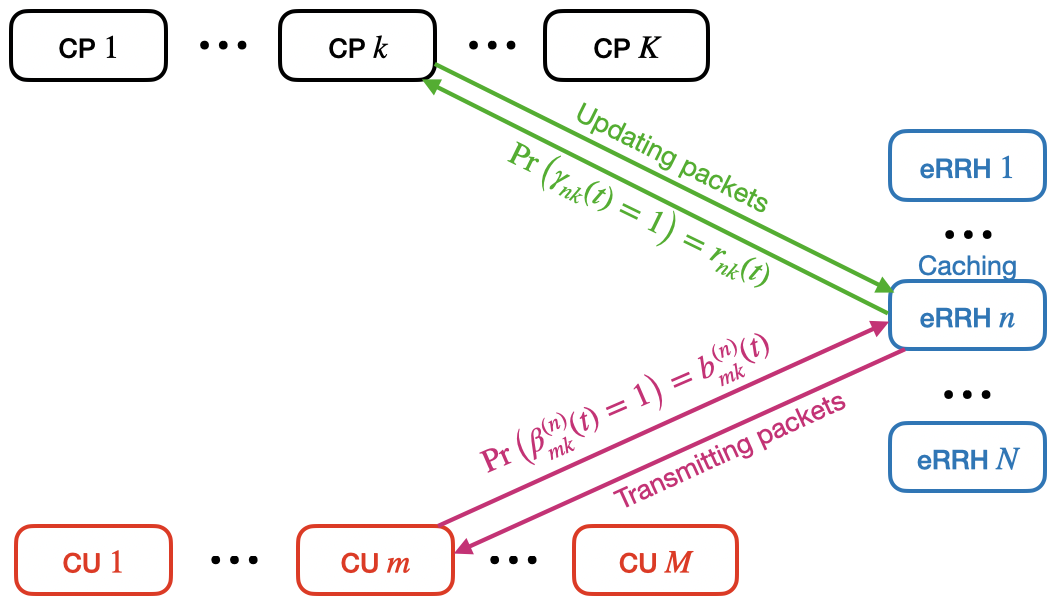
Figure 2: An example of a fog computing-based radio access network.

Let time be slotted, with each time slot spanning several seconds, minutes, hours or even a full day, depending on practice settings. At the beginning of every time slot, CU $m$ decides whether to send a request for packets from CP $k$ to eRRH $n$ or not. Denote $\beta_{mk}^{(n)}(t)\in\{0,1\}$, $m\in[M]$, $n\in[N]$, $k\in[K]$; $\beta_{mk}^{(n)}(t)=1$ indicates that CU $m$ send a request for CP $k$ to eRRH $n$ and $\beta_{mk}^{(n)}(t)=0$ otherwise. Furthermore, for every $k$, CU $m$ sends at most one request, i.e., for all $m,k,t$,

$$\sum_{n\in[N]}\beta_{mk}^{(n)}(t)\leq 1.$$ (1)

It is worth noting that $\{\beta_{mk}^{(n)}(t)\}_{n}$ are not independent over $n$. This setting differs from those in cache updating systems as discussed in [9, 10, 8, 11, 12], where the counterpart variables are independent over $n$. This inter-dependence in our model introduces additional complexity compared to the aforementioned studies. Denote the probability/rate of each action as

$$\Pr\big{(}\beta_{mk}^{(n)}(t)=1\big{)}\triangleq b_{mk}^{(n)}(t)\in[0,1].$$ (2)

From (1) and (2), we have

$$\sum_{n\in[N]}b_{mk}^{(n)}(t)\leq 1,$$ (3)

for all $m,k,t$. CU $m$ sends a request in time slot $t$ with rate $\sum_{n\in[N]}b_{mk}^{(n)}(t)$.

Upon receiving requests from CUs, eRRH $n$ can either command CP $k$ to update with a new packet or retrieve a previously cached packet. Let $\gamma_{nk}(t)\in\{0,1\}$ represent the command of eRRH $n$ for CP $k$ at time slot $t$, given that $\sum_{m\in[M]}\beta_{mk}^{(n)}(t)\geq 1$. If $\gamma_{nk}(t)=1$, eRRH $n$ commands CP $k$ to send a new packet; otherwise, $\gamma_{nk}(t)=0$, indicating that the eRRH uses the cached packet. $\{\gamma_{nk}(t)\}_{k}$ are independent over $k$. Let

$$\Pr(\gamma_{nk}(t)=1)\triangleq r_{nk}(t)\in[0,1].$$ (4)

Recall that we consider decentralized strategies, so $\{\beta_{mk}^{(n)}(t)\}$ is independent over $m$. Then, eRRH $n$ gets new a packet from CP $k$ in time slot $t$ with probability

$$\big{(}1-\prod_{m\in[M]}(1-b_{mk}^{(n)}(t))\big{)}r_{nk}(t),$$ (5)

which reflects the decentralized nature of the decision-making process in the network.

Next, we display several key assumptions in our setting: (i) Requests from CUs and commands from eRRHs are small in size, making the transmission delays negligible, (ii) The transmission delays of packets from CPs to eRRHs are fixed at one time slot, while the transmission delays of packets from eRRHs to CUs are negligible. (iii) We do not assume interference in transmissions, following the precedents [9, 10, 11, 12, 8]. In fact, interference can be avoided utilizing advanced techniques, such as power-domain non-orthogonal multiple access. Let $B$ represent the constraints on the actions of each CU, which include the limitations of ratio resources (e.g., bandwidth) and the demand from external environments. Given that CUs are statistically identical within their groups, we impose the following constraint: constraints:

$$\sum_{n\in[N]}\sum_{k\in[K]}b_{mk}^{(n)}(t)\leq B,\,\,\text{for }m\in[M].$$ (6)

A small $B$ implies that the demand for content from CPs is low or that ratio resources are limited, otherwise $B$ is large, while a large $B$ indicates high demand or ample radio resources. Similarly, let $R$ represent the constraints on the actions of each eRRH, reflecting the resources available on the eRRHs’ side,

$$\sum_{k\in[K]}r_{nk}(t)\leq R,\,\,\text{for }n\in[N].$$ (7)

II-A Age of Information

Packets can be received by both CUs and eRRHs. Accordingly, we define two types of AoI, the AoI at the eRRHs’ side and the AoI at the CUs’ side. By convention, the AoI evolves at the end of each time slot [6, 7, 22].

In time slot $t$, the most recently received packet from CP $k$ cached locally at eRRH $n$ has the generation time $\tau_{nk}$. The AoI of CP $k$ at eRRH $n$ is defined as

$$g_{nk}(t)=t-\tau_{nk}.$$

Recall that the transmission delays of packets from CPs to eRRHs are fixed to be one time slot, so $g_{nk}(t)$ evolves as

$$g_{nk}(t+1)=\left\{\begin{aligned} &1&&\gamma_{nk}(t)\sum_{m\in[M]}\beta_{mk}^{(n)}(t)>0\\ &g_{nk}(t)+1&&\text{otherwise},\end{aligned}\right.$$ (8)

with $g_{nk}(0)=1$.

In time slot $t$, the most recently received packet from CP $k$ has the generation time $\tau^{\prime}_{mk}$. The AoI of CP $k$ at CU $m$ is defined as

$$h_{mk}(t)=t-\tau_{mk}^{\prime}.$$

To ensure the information freshest, if a delivered packet is older than the most recently received one, it will be discarded. Therefore, from (1), $h_{mk}(t)$ evolves as

$$h_{mk}(t+1)=\left\{\begin{aligned} &1&&\text{if }\beta_{mk}^{(n)}(t)\gamma_{nk}(t)=1\\ &\tilde{h}_{mk}^{(n)}(t)+1&&\text{if }\beta_{mk}^{(n)}(t)\big{(}1-\gamma_{nk}(t)\big{)}=1\\ &h_{mk}(t)+1&&\sum_{n}\beta_{mk}^{(n)}(t)=0,\end{aligned}\right.$$ (9)

with $\tilde{h}_{mk}^{(n)}(t)=\min\{h_{mk}(t),g_{nk}(t)\}$ and $h_{mk}(0)=1$. The inter-dependence of decisions within each CU is implied by (1) and (9), meaning the age of version metric introduced in [9, 10, 8, 11, 12] cannot be applied.

Based on (8) and (9), we calculate the average AoI of eRRHs and CUs, respectively. The average AoI of eRRHs is defined as

$$J_{e}=\lim_{T\to\infty}\frac{1}{T}\sum_{t=1}^{T}\frac{1}{NK}\sum_{n\in[N]}\sum_{k\in[K]}\mathbb{E}[g_{nk}(t)].$$ (10)

Similarly, the average AoI of CUs is defined as

$$J_{c}=\lim_{T\to\infty}\frac{1}{T}\sum_{t=1}^{T}\frac{1}{MK}\sum_{m\in[M]}\sum_{k\in[K]}\mathbb{E}[h_{mk}(t)].$$ (11)

II-B Stationary Randomized Policies

We consider decentralized policies for CUs and eRRHs, where each CU and eRRH makes decisions based on its local information. This decentralization implies that $\big{\{}\{\beta_{mk}^{(n)}(t)\}_{n,k}\big{\}}_{m}$ are independent across $m$, and $\big{\{}\{\gamma_{nk}(t)\}_{k}\big{\}}_{n}$ are independent across $n$. We define a decentralized policy as

$$\pi=\Big{\{}\big{\{}\{b_{mk}^{(n)}(t)\}_{n,k}\big{\}}_{m},\big{\{}\{r_{nk}(t)\}_{k}\big{\}}_{n}\Big{\}}_{t}.$$ (12)

For analysis tractability, this paper focuses on a class of widely used decentralized policies, known as stataionary randomized policies, where each action happens with a fixed probability [17, 18]. We first introduce oblivious stationary randomized (OSR) policies, where decisions are independent of AoI history information. Then, we define non-oblivious stationary randomized (NSR) policies, where decisions by eRRHs depend on history information of AoI [7, 22].

II-B1 Oblivious Stationary Randomized Policies

The idea behind OSR policies entails that every node, including CUs and eRRHs, makes decisions based on predetermined probabilities, independent of history information of AoI. Specifically, the decisions of every CU are reduced to

$$b_{mk}^{(n)}(t)=b_{k}^{(n)},\text{ for all }m,t.$$ (13)

For each eRRH $n$, a rate vector $\{r_{1},r_{2},\cdots,r_{K}\}$ is assigned, where $r_{1}\geq r_{2}\geq\cdots\geq r_{K}$. When eRRH $n$ receives requests for CP $k$ in time slot $t$ (i.e., $\sum_{m\in[M]}\beta_{mk}^{(n)}(t)\geq 1$), it then commands CP $k$ with rate $r_{k}$,

$$r_{nk}(t)= r_{k}\cdot 1_{\{\sum_{m\in[M]}\beta_{mk}^{(n)}(t)\geq 1\}}.$$ (14)

Definition 1.

In a network, an O2S strategy is defined by (12), where $\{b_{mk}^{(n)}(t)\}_{m,n,k}$ and $\{r_{nk}(t)\}_{n,k}$ are provided in (13) and (14), respectively.

II-B2 Non-oblivious Stationary Randomized Policies

Under a NSR policy, eRRH $n$ utilizes the history information of AoI to make commanding decisions. A CP with a larger ages is given a higher priority in decision-making. Specifically, in time slot $t$, eRRH $n$ arranges $\{g_{nk}(t)\}_{k\in[K]}$ in descending order: $g_{nl_{1}}(t)\geq g_{nl_{2}}(t)\geq\cdots\geq g_{nl_{K}}(t)$. If eRRH $n$ receives request(s) for CP $l_{k}$, it commands CP $l_{k}$ with rate:

$$r_{nl_{k}}(t)= r_{k}\cdot 1_{\{\sum_{m\in[M]}\beta_{ml_{k}}^{(n)}(t)\geq 1\}}.$$

However, if all CPs have large ages at eRRH $n$, then prioritization among them is unnecessary. In such cases, a predefined threshold $z$ is introduced. If $g_{nl_{K}}(t)\geq z$, then every CP will be commanded with an equal rate. The expression of $r_{nl_{k}}(t)$ is then:

$$r_{nl_{k}}(t)=\left\{\begin{aligned} r_{k}\cdot 1_{\{\sum_{m\in[M]}\beta_{ml_{k}}^{(n)}(t)\geq 1\}}&&g_{nl_{K}}(t)<z\\ r_{0}\cdot 1_{\{\sum_{m\in[M]}\beta_{ml_{k}}^{(n)}(t)\geq 1\}}&&g_{nl_{K}}(t)\geq z,\end{aligned}\right.$$ (15)

where $r_{0}=\frac{1}{K}\sum_{k\in[K]}r_{k}$.

Definition 2.

In a network, a NSR policy is defined by (12), where $\{b_{mk}^{(n)}(t)\}_{m,n,k}$ and $\{r_{nk}(t)\}_{n,k}$ are provided in (13) and (15), respectively.

The policy in Definition 2 allows eRRHs to dynamically adjust commanding rates based on the ages of CPs, promoting efficient resource allocation while maintaining flexibility in handling varying network conditions.

II-B3 Feasible Region

Now, we determine the feasible region of stationary randomized policies. Let $b_{k}\triangleq\sum_{n\in[N]}b_{k}^{(n)}$ represent the rate of a CU sending requests for CP $k$ to eRRHs. Define $b\triangleq\sum_{n\in[N]}\sum_{k\in[K]}b_{k}$ and $r\triangleq\sum_{k\in[K]}r_{k}$. Based on (3), (6), (7), (14), and (15), the feasible region for a stationary randomized policy $\pi$ is

$$\mathcal{F}\triangleq\{(b,r,\{b_{k}\}_{k\in[K]})|b\leq B,r\leq R,b_{k}\leq 1,k\in[K]\}.$$

II-C Optimization Problems

Our goal is to deliver new packets to CUs as quickly as possible. Mathematically, this goal can be modeled by minimizing the average AoI of CUs through a stationary randomized policy, i.e.,

$$\pi^{*}=\min_{\pi}J_{c},$$ (16)

where $\pi$ can be either an OSR or a NSR policy. Given that CUs communicate with CPs through eRRHs, $J_{c}$ is influenced by $J_{e}$. To solve the optimization (16), we follow these $3$ steps: (i) analyze $J_{e}$ theoretically, (ii) analyze $J_{c}$ theoretically, and (iii) determine an optimal strategy $\pi^{*}$ as defined in (16).

In the rest of the paper, we consider $(b,r,\{b_{k}\}_{k\in[K]})\in\mathcal{F}$. First, we analyze $J_{e}$ and $J_{c}$, and derive the O2S and N2S policies for F-RANs with $2$ CUs, $2$ eRRHs, and $2$ CPs in Section III and Section IV, respectively. Then, we generalize the framework and optimal strategies to general networks with $M$ CUs, $N$ eRRHs, and $K$ CPs in Appendix I.

III Optimal OSR Policies

In this section, we investigate an optimal OSR policy in a network with $N=M=K=2$, and the theoretical results presented in this section can be straightforwardly extended to general networks with an arbitrary number of CUs, eRRHs, and CPs (see Appendix I). To achieve this, we start by calculating $J_{e}$ as defined in (10) and derive its closed form of $J_{e}$ (see Theorem 1 in Section III-A). Given the complexity of calculating $J_{c}$, obtaining its closed form is challenging. Instead, we derive two upper bounds for $J_{c}$ (see Theorem 2 in Section III-B). Finally, we solve the optimization (16) and obtain an optimal O2S strategy $\pi^{*}$ (see Theorem 3 in Section III-C).

III-A Closed From of $J_{e}$

From (5), (8) and (14), $g_{nk}(t)$ decreases to $1$ with probability $r_{k}\cdot\big{(}1-(1-b_{k}^{(n)})^{2}\big{)}$. Denote

$$\zeta_{nk}\triangleq 1-(1-b_{k}^{(n)})^{2},$$ (17)

and $\zeta_{nk}$ is a concave function of $b_{k}^{(n)}$. The recursion of $g_{nk}(t)$ in (8) is then given by

$$g_{nk}(t+1)=\left\{\begin{aligned} &1&&\text{w.p. }r_{k}\zeta_{nk}\\ &g_{nk}(t)+1&&\text{w.p. }1-r_{k}\zeta_{nk}.\end{aligned}\right.$$ (18)

We use a graphical argument to calculate the AoI $J_{e}$ [35], as illustrated in Fig. 3.

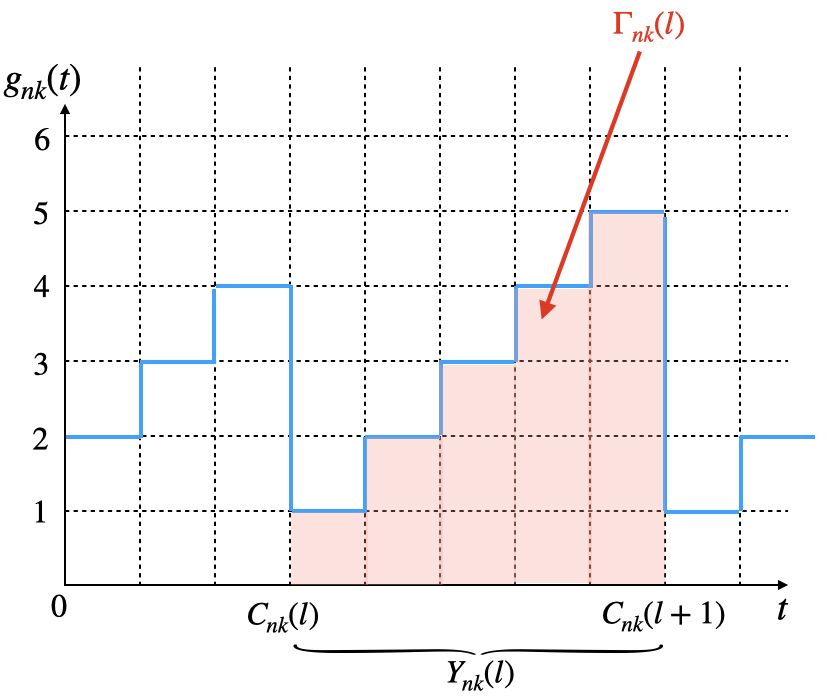
Figure 3: A trajectory of $g_{nk}(t)$.

Let $C_{nk}(l)$ denote the timestamp when eRRH $n$ reiceves a new packet from CP $k$ for the $l$-th time. Let

$$Y_{nk}(l)=C_{nk}(l+1)-C_{nk}(l).$$

Since the transmission delays from CPs and eRRHs are fixed at $1$, we have $g_{nk}(C_{nk}(l))\equiv 1$ for all $l$. Define $\Gamma_{nk}(l)$ as the summation of $g_{nk}(t)$ within $[C_{nk}(l),C_{nk}(l+1))$:

$$\Gamma_{nk}(l)=\sum_{t=C_{nk}(l)}^{C_{nk}(l+1)-1}g_{nk}(t)=\frac{1}{2}Y_{nk}^{2}(l)+\frac{1}{2}Y_{nk}(l).$$

Theorem 1.

Let $\zeta_{nk}$ be given in (17). The closed-form expression for the average AoI of eRRHs is provided by

$$J_{e}=\frac{1}{4}\sum_{n\in[2]}\sum_{k\in[k]}\frac{\mathbb{E}[\Gamma_{nk}(l)]}{\mathbb{E}[Y_{nk}(l)]}=\frac{1}{4}\sum_{n\in[2]}\sum_{k\in[k]}\frac{1}{r_{k}\zeta_{nk}}.$$ (19)

Remark 1.

It is straightforwad to verify that (19) is convex with respect to $r_{1}$ and $r_{2}$. Consequently, given decisions of CUs $\{b_{k}^{(n)}\}_{n,k}$, there exists a unique optimal $\{r_{k}\}_{k\in[2]}$ [36].

Proof.

The proof is given in Appendix A. ∎

III-B Upper Bounds of $J_{c}$

From (9), (13), and (14), we simplify the recursion of $h_{mk}(t)$ as follows:

$$h_{mk}(t+1)=\left\{\begin{aligned} &1&&b_{k}r_{k}\\ &\min\{h_{mk}(t),g_{1k}(t)\}+1&&b_{k}^{(1)}(1-r_{k})\\ &\min\{h_{mk}(t),g_{2k}(t)\}+1&&b_{k}^{(2)}(1-r_{k})\\ &h_{mk}(t)+1&&1-b_{k}.\end{aligned}\right.$$ (20)

Since $\beta_{mk}^{(1)}(t)$ and $\beta_{mk}^{(1)}(t)$ (defined in Section II) are not independent, the $\min\{\cdot\}$ function in (20) complicates the analysis of $J_{c}$, making it challenging to derive a closed form. Therefore, we aim to obtain two upper bounds for $J_{c}$.

Theorem 2.

Let $\zeta_{nk}$ be given in (17). Then, $J_{c}$ has two upper bounds,

$$J_{c}\leq \frac{1}{2}\sum_{k\in[2]}\frac{1}{b_{k}r_{k}},$$ (21)

$$J_{c}\leq \frac{1}{2}\sum_{k\in[2]}\Big{(}\frac{1-b_{k}+b_{k}r_{k}}{b_{k}r_{k}}+\sum_{n=1}^{2}\frac{b_{k}^{(n)}(1-r_{k})}{r_{k}\zeta_{nk}}\Big{)}.$$ (22)

Proof.

The proof is given in Appendix B. ∎

The upper bound in (21) represents the average AoI in an extreme scenario where eRRHs only send new packets and do not transmit previously cached ones. The upper bound in (22) reflects the average AoI in an extreme case where CUs replace the most recently received packets with the current delivered packets from eRRHs, even if they are older. When $b_{k}^{(1)}$ and $b_{k}^{(2)}$ are significantly different, i.e., $|b_{k}^{(1)}-b_{k}^{(2)}|\approx b_{k}$, the second upper bound (22) becomes large, making the first upper bound (21) a better estimate. Conversely, when $b_{k}^{(1)}$ and $b_{k}^{(2)}$ are close to each other, i.e., $b_{k}^{(1)}\approx b_{k}^{(2)}\approx b_{k}/2$, the second upper bound (22) provides a better estimate (see Fig. 6 in Section V).

III-C Optimal OSR Strategy

Now, we aim to obtain an optimal policy $\pi^{*}$ for $J_{c}$ in (11). To achieve this, we follow two steps: (i) Fix $b_{k}$ and $r_{k}$, determine an optimal $\big{(}(b_{k}^{(1)})^{*},(b_{k}^{(2)})^{*}\big{)}$ that minimize

$$\lim_{T\to\infty}\frac{1}{T}\sum_{t=1}^{T}\mathbb{E}[h_{mk}(t)];$$

(ii) Find an optimal policy $\pi^{*}$ to minimize

$$J_{c}=\frac{1}{4}\sum_{m\in[2]}\sum_{k\in[2]}\lim_{T\to\infty}\frac{1}{T}\sum_{t=1}^{T}\mathbb{E}[h_{mk}(t)].$$

By systematically addressing these steps, we identify a policy that optimally minimizes the average AoI for the CUs.

From (20), we derive the following two observations for $h_{mk}(t)$ that help us to understand an optimal $\big{(}(b_{k}^{(1)})^{*},(b_{k}^{(2)})^{*}\big{)}$. (i) When $b_{k}$ is small: This means CU $m$ sends a request for CP $k$ with a samll rate. Assuming $b_{k}^{(1)}\geq b_{k}^{(2)}$, $\mathbb{E}[h_{mk}(t)]$ is likely to be larger than $\mathbb{E}[g_{1k}(t)]$. Therefore, $\mathbb{E}[h_{mk}(t)]$ is primarily determined by $\{g_{1k}(l)\}_{l\leq t}$. In this scenario, an optimal choice is $(b_{k}^{(1)},b_{k}^{(2)})=(b_{k},0)$. (ii) When $b_{k}$ is large, for instance, $b_{k}\approx 1$, CU $m$ sends a request for CP $k$ with a high rate. Since $g_{nk}(t)$ follows a geometric distribution, which is light-tailed, the probability of encountering high $g_{nk}(t)$ (and hence high $h_{mk}(t)$) is small. Then, the min function in (20) becomes significant, and both $g_{nk}(t)$ with $n\in\{1,2\}$ affect $h_{mk}(t)$. Here, an optimal choice is $(b_{k}^{(1)},b_{k}^{(2)})=(b_{k}/2,b_{k}/2)$.

We define two stochastic processes,

$$H_{mk,1}(t+1)=\left\{\begin{aligned} &1&&b_{k}r_{k}\\ &h_{mk}(t)+1&&1-b_{k}r_{k};\end{aligned}\right.$$ (23)

and

$$H_{mk,2}(t+1)=\left\{\begin{aligned} &1&&b_{k}r_{k}\\ &g_{1k}(t)+1&&b_{k}^{(1)}(1-r_{k})\\ &g_{2k}(t)+1&&b_{k}^{(2)}(1-r_{k})\\ &h_{mk}(t)+1&&1-b_{k},\end{aligned}\right.$$ (24)

with $H_{mk,1}(0)=H_{mk,2}(0)=1$. From (20), (23), and (24),

$$h_{mk}(t)\overset{d}{=}\min\{H_{mk,1}(t),H_{mk,2}(t)\}$$ (25)

where $\overset{d}{=}$ represents equality in distribution. By utilizing (25), we derive the following analytical results.

Lemma 1.

Fix $b_{k}$ and $r_{k}$. There exists a threshold depending on $r_{k}$, denoted as $w(r_{k})\in[0,1]$, such that: (i) when $w(r_{k})<b_{k}\leq 1$, $(b_{k}^{(1)},b_{k}^{(2)})=(b_{k}/2,b_{k}/2)$ is a global minimum point of $\mathbb{E}[h_{mk}(t)]$; (ii) when $0<b_{k}\leq w(r_{k})$, $(b_{k}^{(1)},b_{k}^{(2)})=(b_{k},0)$ or $(0,b_{k})$ is a global minimum point of $\mathbb{E}[h_{mk}(t)]$.

Proof.

The proof is given in Appendix C. ∎

Based on Lemma 1, we provide insights into an optimal choice for distributing request rates $b_{k}$ among eRRHs under various conditions. From the definitions of $h_{mk}(t)$, it is evident that $h_{mk}(t)$ is an asymptotically stationary process under stationary randomized policies [37]. Thus, the initial point $h_{mk}(0)$ has a negligible impact on $h_{mk}(t)$ when $t$ becomes large. As established in [37, Eqn. (15)], we have

$$\lim_{T\to\infty}\frac{1}{T}\sum_{t=1}^{T}\mathbb{E}[h_{mk}(t)]=\lim_{t\to\infty}\mathbb{E}[h_{mk}(t)].$$

Given that $b_{k}$ and $r_{k}$ are fixed, we observe the following:

• (i) When the rate of a CU sending a request for CP $k$ to eRRHs is relatively small, i.e., $0<b_{k}<w(r_{k})$, either $(b_{k}^{(1)},b_{k}^{(2)})=(b_{k},0)$ or $(0,b_{k})$ is a global minimum point of $\lim_{t\to\infty}\mathbb{E}[h_{mk}(t)]$. In this case, an optimal choice is to consolidate all rates to single eRRH.

• (ii) When the rate of a CU sending a request for CP $k$ to eRRHs is relatively large, i.e., $w(r_{k})<b_{k}\leq 1$, $(b_{k}^{(1)},b_{k}^{(2)})=(b_{k}/2,b_{k}/2)$ is a global minimum point of $\lim_{t\to\infty}\mathbb{E}[h_{mk}(t)]$. In this case, an optimal choice is to allocate the rate $b_{k}$ equally to both eRRHs.

• (iii) If we relax the condition (1) such that $\beta_{mk}^{(n)}(t)$ are independent across $n$, then using Step 2 of the proof in Appendix D, we obtain the same conclusions as in [10, 11, 8]. That is, the optimal choice is to consolidate all rates to single eRRH.

Lemma 2.

Let $b,r$ be fixed and $(b,r)\in\mathcal{F}$, $(b_{k},r_{k})=(b/2,r/2)$ is a global minimum point of $\sum_{k\in[2]}\mathbb{E}[h_{mk}(t)]$.

Proof.

The proof is given in Appendix D. ∎

From Lemma 1 and Lemma 2, we conclude that for each CU, the optimal decision for allocating rates among CPs is an equal distribution, regardless of how rates are allocated within the eRRHs associated with each CP. Similarly, for each eRRH, the optimal decision for allocating rates among CPs is to distribute them equally.

Theorem 3.

Let $b,r$ be fixed, $(b,r)\in\mathcal{F}$, and $m,n,k\in[2]$. there exists a threshold (depending on $r$), $w(\frac{r}{2})\in[0,1]$, such that if $\frac{b}{2}>w(\frac{r}{2})$, an optimal policy $\pi^{*}$ is given by

$$\pi^{*}=\{b_{mk}^{(n)}=b/4,r_{k}=r/2\};$$ (26)

if $\frac{b}{2}\leq w(\frac{r}{2})$, an optimal policy

$$\pi^{*}=\{ (b_{mk}^{(n)},b_{mk}^{(3-n)})=(b/2,0),r_{k}=r/2\}.$$ (27)

Proof.

The proof follows directly from Lemma 1 and Lemma 2. ∎

In Theorem 3, obtaining the closed form of $w(\frac{r}{2})$ is extremely challenging. However, given that the sequence ${h_{mk}(t)}_{t}$ is asymptotically stationary, for small values of $t$, $w\left(\frac{r}{2}\right)$ can be estimated. For example, as discussed in Step 1 of Appendix C, by setting $t=2$,

$$w(\frac{r}{2})\approx\frac{2}{3-r/2}.$$ (28)

When $\frac{b}{2}$ is significantly larger than $\frac{2}{3-r/2}$, an optimal policy is given in (26), when $\frac{b}{2}$ is significantly smaller than $\frac{2}{3-r/2}$, an optimal policy is given in (27), and when $\frac{b}{2}$ is approximately equal to $\frac{2}{3-r/2}$, the average AoI of CUs under both policies given in (26) and (27) do not differ significantly.

IV Optimal NSR Policies

In this section, we investigate an optimal NSR policy in a network with $N=M=K=2$, following a process similar to the one described in Section III. The theoretical results presented in this section can be straightforwardly extended to general networks with an arbitrary number of CUs, eRRHs, and CPs (see Appendix I). we begin by calculating $J_{e}$ as defined in (10) and derive its closed form of $J_{e}$ (see Theorem 4 in Section IV-A) through introducing a two-dimensional truncated Markov chain in (see (32)). Next, derive two upper bounds for $J_{c}$ (see Theorem 5 in Section IV-B). Finally, we theoretically determine an optimal strategy $\pi^{*}$ (see Theorem 6) in Section IV-C.

IV-A Closed From of $J_{e}$

From (15), the recursions of $g_{n1}(t)$ and $g_{n2}(t)$ are correlated with each other in every time slot $t$. Let $G_{n}(t)=(g_{n1}(t),g_{n2}(t))$, and denote the whole space of $G_{n}(t)$ as $\mathcal{G}_{n}$. The space $\mathcal{G}_{n}$ can be partitioned in the following $3$ disjoint subsets (see Fig. 4),

$$\mathcal{G}_{n1}= \Big{\{}G_{n}(t)|g_{n1}(t)\geq g_{n2}(t),g_{n2}(t)<z,t\geq 0\Big{\}},$$

$$\mathcal{G}_{n2}= \Big{\{}G_{n}(t)|g_{n1}(t)<g_{n2}(t),g_{n1}(t)<z,t\geq 0\Big{\}},$$

$$\mathcal{G}_{n3}= \Big{\{}G_{n}(t)|\{g_{n1}(t)\geq z,g_{n2}(t)\geq z,t\geq 0\Big{\}}.$$

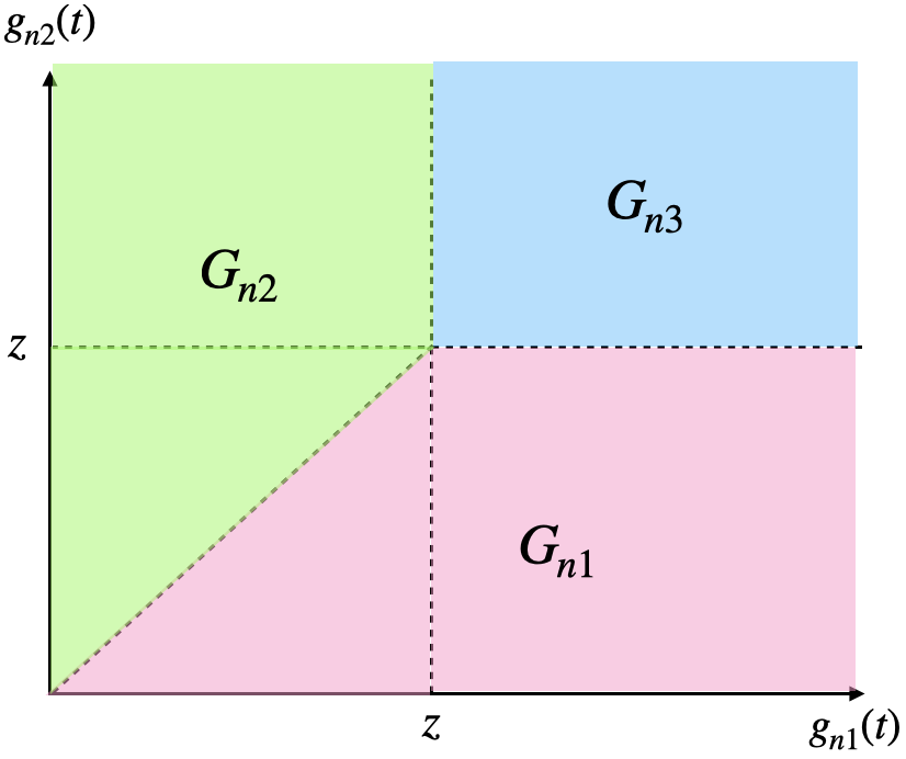
Figure 4: The partition of $\mathcal{G}_{n}$.

For $n,k\in[2]$, according to (4), the rate $r_{nk}(t)=\Pr\{\gamma_{nk}(t)=1\}$ depends on the values of $G_{n}(t)$ and changes over time. Based on (15), we obtain

$$r_{nk}(t)= 1_{\{G_{n}(t)\in\mathcal{G}_{n1}\}}r_{k}+1_{\{G_{n}(t)\in\mathcal{G}_{n2}\}}(r-r_{k})$$

$$+ 1_{\{G_{n}(t)\in\mathcal{G}_{n3}\}}r/2$$ (29)

Then, the recursion of $g_{nk}(t)$ is given by

$$g_{nk}(t+1)=\left\{\begin{aligned} &1&&\text{w.p. }r_{nk}(t)\zeta_{nk}\\ &g_{nk}(t)+1&&\text{w.p. }1-r_{nk}(t)\zeta_{nk},\end{aligned}\right.$$ (30)

where $\zeta_{nk}$ is given in (17).

Similar to [37, Eqn. (13)], we define for any time slot $t$,

$$X_{nk}(t)=\min\{C_{nk}(l)|C_{nk}(l)>t\}-t,$$ (31)

where $C_{nk}(l)$ represents the timestamp when eRRH $n$ receives a new packet from CP $k$ for the $l$-th time, as defined in Section III-A. In other words, $X_{nk}(t)$ in (31) denotes the time period from time slot $t$ to the next update. According to [37, Eqn. (15)],

$$\lim_{T\to\infty}\frac{1}{T}\sum_{t=1}^{T}\mathbb{E}[g_{nk}(t)]=\lim_{t\to\infty}\mathbb{E}[X_{nk}(t)]\quad\text{with probability }1.$$

Thus, $J_{e}$ in (10) can be re-written as

$$J_{e}=\frac{1}{4}\sum_{n\in[2]}\sum_{k\in[2]}\lim_{t\to\infty}\mathbb{E}[X_{nk}(t)]\quad\text{with probability }1.$$

The remainder of this section focuses on calculating $\mathbb{E}[X_{nk}(t)]$.

Note that the state space $\mathcal{G}_{n}$ is infinite, to obtain the closed form of $J_{e}$, we introduce another vector $G_{n}^{z}(t)$, representing the $z$-truncated age state of eRRHs in time slot $t$ [37]:

$$G_{n}^{z}(t)=(g_{n1}^{z}(t),g_{n2}^{z}(t)),$$ (32)

where $g_{nk}^{z}(t)$ is truncated at $z$. The evolution of $g_{nk}^{z}(t)$ is defined as follows

$$g_{nk}^{z}(t+1)=\left\{\begin{aligned} &1&&\text{w.p. }r_{nk}(t)\zeta_{nk}\\ &\min\{g_{nk}^{z}(t)+1,z\}&&\text{w.p. }1-r_{nk}(t)\zeta_{nk}.\end{aligned}\right.$$

From [37, Proposition 1] and [37, Proposition 2], we know that $G_{n}^{z}(t)$, as defined in (32), is a Morkov process and possesses a unique steady-state distribution. The state space of $G_{n}^{z}(t)$ is given by

$$\mathcal{G}_{n}^{z}=\{\phi|G_{n}^{z}(t)=\phi,t\geq 0\},$$

with the cardinality $|\mathcal{G}_{n}^{z}|=z^{2}$. The steady-state distribution, denoted as $\pi=\{\pi_{\phi}\}_{\phi\in\mathcal{G}_{n}^{z}}$, is uniquely determined by

$$\pi={\bf P}\pi,$$ (33)

where ${\bf P}$ is the transition probability matrix. The specific form of ${\bf P}$ is provided in (66), (67), (68), and (69) in Appendix E.

We proceed to derive the closed form of $J_{e}$ using $G_{n}^{z}(t)$ defined in (32). Following a similar approach as in [37, Eqn. (25)], we express the expected age $\mathbb{E}[X_{nk}(t)]$ as

$$\mathbb{E}[X_{nk}(t)]= \sum_{\phi\in\mathcal{G}_{n}^{z}}\mathbb{E}[X_{nk}(t)|G_{n}^{z}(t)=\phi]\Pr(G_{n}^{z}(t)=\phi)$$

$$\triangleq \sum_{\phi\in\mathcal{G}_{n}^{z}}F_{nk}(\phi)\pi_{\phi},$$ (34)

where $F_{nk}(\phi)=\mathbb{E}[X_{nk}(t)|G_{n}^{z}(t)=\phi]$ denotes the expected time until the next new packet from CP $k$, given the AoI state $\phi=(\phi_{1},\phi_{2})$. Define the set $\mathcal{G}_{n,down,k}$ as

$$\mathcal{G}_{n,down,k}=\{\phi|\phi\in\mathcal{G}_{n}^{z},\phi_{k}=1\},\,\,k\in[2].$$ (35)

Here, $F_{nk}(\phi)$ represents the mean first passage time through a state $\mathcal{G}_{n,down,k}$ starting from state $\phi$. The transition probabilities $P_{\phi\phi^{\prime}}$ (see (66), (67), (68), and (69) in Appendix E) indicate the probability of transitioning from state $\phi$ to state $\phi^{\prime}$. Similar to the derivations in [37, Eqns. (28) and (29)], the mean first passage times starting from each state $\phi$, can be determined by using one-step analysis, i.e., by solving the system of equations,

$$F_{nk}(\phi)=1+\sum_{\phi^{\prime}\in\mathcal{G}_{n}^{z}\backslash\mathcal{G}_{n,down,k}}{\bf P}_{\phi\phi^{\prime}}F_{nk}(\phi^{\prime}),\,\,\phi\in\mathcal{G}_{n}^{z}.$$ (36)

By leveraging (33), (IV-A), and (36), we directly establish the following theorem.

Theorem 4.

The closed-form expression for the average AoI of eRRHs is provided by

$$J_{e}=\frac{1}{4}\sum_{n\in[2]}\sum_{k\in[2]}\sum_{\phi\in\mathcal{G}_{n}^{z}}F_{nk}(\phi)\pi_{\phi},$$ (37)

where $\pi_{\phi}$ is provided by (33) and $F_{nk}(\phi)$ is provided by (36).

IV-B Upper Bounds of $J_{c}$

From (9) and (29), under a NSR policy, $h_{mk}(t)$ has the following recursion,

$$h_{mk}(t+1)=\left\{\begin{aligned} &1,\quad\sum_{n\in[2]}b_{k}^{(n)}r_{nk}(t)\\ &\min\{h_{mk}(t),g_{1k}(t)\}+1,\,\,b_{k}^{(1)}(1-r_{1k}(t))\\ &\min\{h_{mk}(t),g_{2k}(t)\}+1,\,\,b_{k}^{(2)}(1-r_{2k}(t))\\ &h_{mk}(t)+1,\quad 1-b_{k},\end{aligned}\right.$$ (38)

where $g_{1k}(t)$ and $g_{2k}(t)$ are given in (30). Similar to Section III-B, we provide two upper bounds of $J_{c}$.

Theorem 5.

$J_{c}$ defined in (11) have two upper bounds,

$$J_{c}\leq \frac{1}{2}\sum_{k\in[2]}\frac{1}{b_{k}r_{2}},$$ (39)

$$J_{c}\leq \frac{1}{2}\sum_{k\in[2]}\Big{(}\frac{1-b_{k}+b_{k}r_{2}}{b_{k}r_{2}}$$

$$+(1-r_{2})\sum_{n\in[2]}b_{k}^{(n)}\sum_{\phi\in\mathcal{G}_{n}^{z}}F_{nk}(\phi)\pi_{\phi}\Big{)}.$$ (40)

Proof.

The proof is given in Appendix F. ∎

Both upper bounds (39) and (40) represent the extreme scenatio where eRRHs always command CPs to update new packets with probability $r_{2}$. In addition, in the case associated with (39), CUs exclusively send new packets without transmitting previously cached ones; while in the case associated with (40), CUs replace the most recently received packets with the current delivered by eRRHs, even if they are older. Similar to Theorem 2, when $b_{k}^{(1)}$ and $b_{k}^{(2)}$ are significantly different, the first upper bound (39) provides a more accurate estimate; while $b_{k}^{(1)}$ and $b_{k}^{(2)}$ are close to each other, the second upper bound (40) serves as a better estimate (see Fig. 7 in Section V).

IV-C Optimal NSR Strategy

Utilizing the approach outlined in Section III-C, we obtain an optimal policy $\pi^{*}$ for $J_{c}$ in (11) through the following two steps: (i) Fix $b_{k}$ and $r_{k}$, determine an optimal $\big{(}(b_{k}^{(1)})^{*},(b_{k}^{(2)})^{*}\big{)}$ that minimize

$$\lim_{T\to\infty}\frac{1}{T}\sum_{t=1}^{T}\mathbb{E}[h_{mk}(t)];$$

(ii) Find an optimal policy $\pi^{*}$ to minimize

$$J_{c}=\frac{1}{4}\sum_{m\in[2]}\sum_{k\in[2]}\lim_{T\to\infty}\frac{1}{T}\sum_{t=1}^{T}\mathbb{E}[h_{mk}(t)].$$

We define two stochastic processes,

$$H_{mk,1}^{\prime}(t+1)=\left\{\begin{aligned} &1&&\sum_{n\in[2]}b_{k}^{(n)}r_{nk}(t)\\ &h_{mk}(t)+1&&1-\sum_{n\in[2]}b_{k}^{(n)}r_{nk}(t)\end{aligned}\right.$$ (41)

and

$$H_{mk,2}^{\prime}(t+1)=\left\{\begin{aligned} &1&&\sum_{n\in[2]}b_{k}^{(n)}r_{nk}(t)\\ &g_{1k}(t)+1&&b_{k}^{(1)}\big{(}1-r_{1k}(t)\big{)}\\ &g_{2k}(t)+1&&b_{k}^{(2)}\big{(}1-r_{2k}(t)\big{)}\\ &h_{mk}(t)+1&&1-b_{k},\end{aligned}\right.$$ (42)

where $g_{1k}(t)$ and $g_{2k}(t)$ are given in (30). By convention, let $H_{mk,1}^{\prime}(0)=H_{mk,2}^{\prime}(0)=1$. From (38), (41), and (42), we have

$$h_{mk}(t)\overset{d}{=}\min\{H_{mk,1}^{\prime}(t),H_{mk,2}^{\prime}(t)\},$$ (43)

where $\overset{d}{=}$ represents equality in distribution. By utilizing (43), we derive the following analytical results.

Lemma 3.

Fix $b_{k},r_{k}$ with $k\in[2]$, there exists a threshold depending on $r_{1}$ and $r_{2}$, denoted as $w^{\prime}(r_{1},r_{2})\in[0,1]$, such that: (i) if $w^{\prime}(r_{1},r_{2})<b_{k}\leq 1$, $(b_{1}^{(1)},b_{1}^{(2)},b_{2}^{(1)},b_{2}^{(2)})=(b_{1}/2,b_{1}/2,b_{2}/2,b_{2}/2)$ is a global minimum point of $\mathbb{E}[h_{mk}(t)]$; (ii) if $0<b_{k}\leq w^{\prime}(r_{1},r_{2})$, either $(b_{1}^{(1)},b_{1}^{(2)},b_{2}^{(1)},b_{2}^{(2)})=(b_{1},0,b_{2},0)$ or $(0,b_{1},0,b_{2})$ is a global minimum point of $\mathbb{E}[h_{mk}(t)]$.

Proof.

The proof is given in Appendix G. ∎

From (29), $r_{nk}(t)$ depends on $(b_{1}^{(1)},b_{1}^{(2)},b_{2}^{(1)},b_{2}^{(2)})$, indicating that $h_{mk}(t)$ is a function of these variables. An optimal distribution of rates $b_{k}$ among eRRHs under NSR policies mirrors that under OSR policies. Specifically, if the rates of CU $m$ sending requests for CP $k$ to eRRHs is relatively small, i.e., $0<b_{k}<w^{\prime}(r_{1},r_{2})$, then either $(b_{1}^{(1)},b_{1}^{(2)},b_{2}^{(1)},b_{2}^{(2)})=(b_{1},0,b_{2},0)$ or $(0,b_{1},0,b_{2})$ serves as a global minimum point for $\lim_{t\to\infty}\mathbb{E}[h_{m1}(t)]$. In such scenarios, an optimal choice is to consolidate all rates for each CP to a single eRRH. Conversely, when the rates is relatively large, i.e., $w^{\prime}(r_{1},r_{2})<b_{k}$, the configuration $(b_{1}^{(1)},b_{1}^{(2)},b_{2}^{(1)},b_{2}^{(2)})=(b_{1}/2,b_{1}/2,b_{2}/2,b_{2}/2)$ emerges as a global minimum point for $\lim_{t\to\infty}\mathbb{E}[h_{mk}(t)]$. In this case, an optimal choice is to equally allocate the rates $b_{1}$ and $b_{2}$ between both eRRHs.

Lemma 4.

Let $b,r$ be fixed and $(b,r)\in\mathcal{F}$, $(b_{1},b_{2})=(b/2,b/2)$ and $(r_{1},r_{2})=(r,0)$ is a global minimum point of $\sum_{k\in[2]}\mathbb{E}[h_{mk}(t)]$.

Proof.

The proof is given in Appendix H. ∎

Theorem 6.

Let $b,r$ be fixed, $(b,r)\in\mathcal{F}$, and $m,n,k\in[2]$. There exists a threshold $w^{\prime}(r,0)\in[0,1]$, such that if $\frac{b}{2}>w^{\prime}(r,0)$, an optimal policy $\pi^{*}$ is given by

$$\pi^{*}=\{b_{mk}^{(n)}=b/4,(r_{1},r_{2})=(r,0)\};$$ (44)

if $\frac{b}{2}\leq w^{\prime}(r,0)$, an optimal policy

$$\pi^{*}=\{ (b_{mk}^{(n)},b_{mk}^{(3-n)})=(b/2,0),(r_{1},r_{2})=(r,0)\}.$$ (45)

Proof.

The proof follows directly from Lemma 3 and Lemma 4. ∎

Unlike an optimal OSR policy, the rates $(r_{1},r_{2})$ are no longer distributed equally. Instead, we have $(r_{1},r_{2})=(r,0)$, meaning all rates are consolidated to the CP with the highest age in a time slot. This approach is optimal because the rates of commands vary with the current ages of the CPs, and thus, the best utilization of rates is to allocate them entirely to the CP with the highest age.

V Numerical Results

In this section, we verify our findings through simulations, focusing on networks with $M=N=K=2$. For non-oblivious policies, we let pre-determined threshold $z=3$.

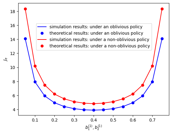
Figure 5: The theoretical and nemerical $J_{e}$ under both oblivious and non-oblivious policies.

In Fig. 5, we validate our theoretical results for $J_{e}$ under both oblivious (see Theorem 1) and non-oblivious (see Theorem 4) policies. For both cases, we let $r_{1}=0.4$, $r_{2}=0.2$, and $b_{1}=b_{2}=0.8$, while varying $b_{1}^{(1)}=b_{2}^{(1)}$ within the range $[0,0.8]$. The closed-form expressions for $J_{e}$ align perfectly with the simulation results, confirming the accuracy of Theorem 1 and Theorem 4. One may observe that $J_{e}$ under the non-oblivious policy is worse than that under the oblivious policy when model parameters are the same. This does not contradict our results, as model parameters impact the performance of age. For example, if we set $r_{1}=0.6$ and $r_{2}=0$, then the non-oblivious policy outperforms the oblivious policy.

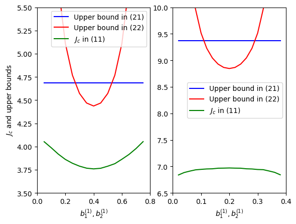
Figure 6: $J_{c}$ and upper bounds under oblivious policies.

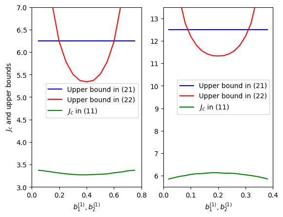
Figure 7: $J_{c}$ and upper bounds under non-oblivious policies.

In Fig. 6 and Fig. 7, we verify our theoretical results for upper bounds (see Theorem 2 and Theorem 5). For both cases, we set $r_{1}=0.4$ and $r_{2}=0.2$. In the left figures, $b_{1}^{(1)}=b_{2}^{(1)}$ varies within the range $[0,0.8]$, while in the left figures, $b_{1}^{(1)}=b_{2}^{(1)}$ varies within the range $[0,0.4]$. We observe that (21), (22), (39), and (40) indeed serve as upper bounds. Specifically, recall that the AoI of eRRH $\{g_{nk}(t)\}_{t}$, as defined in (18) and (30), follows light-tailed distributions. The upper bounds (22) and (40) do not incorporate min functions. When $b_{k}^{(1)}$ and $b_{k}^{(2)}$ are significantly different, and as $b_{k}^{(n)}$ decreases, the coresponding $\mathbb{E}[g_{nk}(t)]$ increases exponentially, causing the upper bound to rise rapidly. Conversely, when $b_{k}^{(1)}$ and $b_{k}^{(2)}$ are close, the upper bounds (22) and (40) become more accurate due to the light-tailed distributions.

Fig. 6 and Fig. 7 also illustrate the optimal choices of $\{b_{k}^{(n)}\}_{n,k}$ when $b_{k}$ and $r_{k}$ are fixed, as discussed in Lemma 1 and Lemma 3. From the left side of both figures, when $b_{1}=b_{2}=0.8$ are relatively large, we observe that $J_{c}$ achieves its minimum point at $(b_{k}^{(1)},b_{k}^{(2)})=(b_{k}/2,b_{k}/2)$. This indicates that the optimal choice is to allocate the rate $b_{k}$ equally to both eRRHs. From the right side of both figures, when $b_{1}=b_{2}=0.4$ are relatively small, $J_{c}$ achieves its minimum point at $(b_{k}^{(1)},b_{k}^{(2)})=(b_{k},0)$ for $k\in[2]$ when $b_{1}=b_{2}=0.4$ are relatively small, suggesting that the an optimal choice to consolidate all rates to single eRRH. These results are consistent with Lemma 1 and Lemma 3. Unlike previous studies [9, 10, 11, 12, 8], where the optimal choice is always to consolidate all rates to a single eRRH (or source), our findings include another different choice. In those precedents, decisions within an eRRH are independent of each other, leading to a straightforward consolidation of rates. However, in our model, the interdependence of decisions within an eRRH results in a different optimal choice. This interdependence decreases the average AoI for CUs by adopting this new optimal choice, resulting in better performance compared to the scenarios considered in the aforementioned studies.

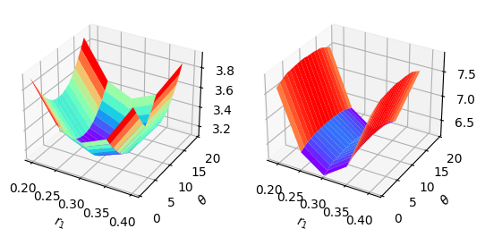
Figure 8: $J_{c}$ under oblivious policies with different $b_{1}$, $b_{2}$, $r_{1}$, and $r_{2}$.

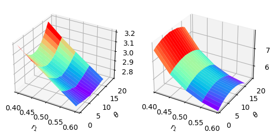
Figure 9: $J_{c}$ under non-oblivious policies with different $b_{1}$, $b_{2}$, $r_{1}$, and $r_{2}$.

In Fig. 8 and Fig. 9, we verify the optimal oblivious and non-oblivious policies as provided in Thoerem 3 and Theorem 6, respectively. In both figures, the $x$-axis represents $r_{1}$, the $y$-axis the index of $b_{k}^{(1)}$ with $k\in[2]$, represented by $\theta\in[20]$, and the $z$-axis represents $J_{c}$. Specifically, when $0\leq\theta\leq 20$, $b_{k}^{(1)}=\frac{b_{k}}{20}\cdot\theta$ with $k\in[2]$. In Fig. 8, we let $(r_{1},r_{2})$ to vary between $[0.2,0.4]$ with $r_{1}+r_{2}=r=0.6$, in the left side of Fig. 8, $(b_{1},b_{2})$ varies within the range $[0.8,1]$ with $b_{1}+b_{2}=b=1.8$, while in the right side, $(b_{1},b_{2})$ varies within the range $[0.3,0.5]$ with $b_{1}+b_{2}=b=0.8$. When $b=0.8$, indicating a relatively low probability of requests for CPs, $J_{c}$ achieves its minimum point at $(b_{1}^{(1)},b_{1}^{(2)},b_{2}^{(1)},b_{2}^{(2)})=(b/2,0,b/2,0)$ and $r_{1}=r_{2}=r/2$; when $b=1.8$, indicating a higher probability of requests for CPs, $J_{c}$ achieves its minimum point at $(b_{1}^{(1)},b_{1}^{(2)},b_{2}^{(1)},b_{2}^{(2)})=(b/4,b/4,b/2,b/4)$ and $r_{1}=r_{2}=r/2$, which are consistent with Theorem 3.

In Fig. 9, we let $r_{1}$ to vary between $[0.4,0.6]$ with $r_{1}+r_{2}=r=0.6$, in the left side of Fig. 9, $(b_{1},b_{2})$ varies within the range $[0.8,1]$ with $b_{1}+b_{2}=b=1.8$, while in the right side, $(b_{1},b_{2})$ varies within the range $[0.3,0.5]$ with $b_{1}+b_{2}=b=0.8$. When $b=0.8$, indicating a relatively low probability of requests for CPs, $J_{c}$ achieves its minimum point at $(b_{1}^{(1)},b_{1}^{(2)},b_{2}^{(1)},b_{2}^{(2)})=(b/2,0,b/2,0)$ and $(r_{1},r_{2})=(r,0)$; when $b=1.8$, indicating a higher probability of requests for CPs, $J_{c}$ achieves its minimum point at $(b_{1}^{(1)},b_{1}^{(2)},b_{2}^{(1)},b_{2}^{(2)})=(b/4,b/4,b/2,b/4)$ and $(r_{1},r_{2})=(r,0)$, which are consistent with Theorem 6.

Comparing Figures 8 and 9, we can observe that the average AoI under an optimal non-oblivious policy is smaller than under an optimal oblivious policy. This is because, in a non-oblivious policy, eRRHs can utilize historical information about the AoI to make more informed decisions. By leveraging this historical data, eRRHs can prioritize updates from CPs with the highest current AoI, thereby optimizing the overall information freshness more effectively than an oblivious policy, which makes decisions without considering past information. Consequently, the ability to incorporate historical AoI data makes the optimal non-oblivious policy more efficient in minimizing the average AoI compared to its oblivious counterpart.

VI Conclusions and Future Research

In this work, we investigated the AoI performance in a decentralized F-RAN consisting $M$ CUs, $N$ eRRHs, and $K$ CPs under two general classes of policies: oblivious and non-oblivious policies. First, we obtained closed-form expressions for the average AoI of eRRHs under both policy types. Due to the complexity in calculating the average AoI of CUs, we derived two general upper bounds for the average AoI of CUs. We then identified optimal oblivious and non-oblivious policies. Under both optimal policies, each CU sends requests to eRRHs for each CP at an equal rate; and consolidates all rates to single eRRH when the demand is low or communication resources are limited, while distributes requests evenly among eRRHs when the demand is high and communication resources are ample. However, the behaviors of eRRHs differ under these policies. In the oblivious case, each eRRH commands content from each CP at an equal rate. In the non-oblivious case, each eRRH consolidates all requests to the CP with the highest age in every time slot. Our numerical results verify these theoretical findings.

Future research includes generalizations to accommodate the following scenarios. 1) Dynamic rates: the probabilities of actions change over time. Addressing this requires the integration of powerful machine learning tools, such as multi-armed bandit algorithms, to adaptively optimize the AoI performance. 2) Heterogeneous networks: Here, CUs, eRRHs, and CPs are no longer statistically identical within their respective groups. A promising approach is to categorize CUs, eRRHs, and CPs into several groups based on their characteristics. We can then apply a similar analytical framework to each group, aggregating the results to identify optimal policies across the heterogeneous network.

Appendix A Proof of Theorem 1

From the definition of $Y_{nk}(l)$, we know that $Y_{nk}(l)$ follows a geometric distribution with parameter $r_{k}\zeta_{nk}$. The first and second moments of $Y_{nk}(l)$ are given by $\mathbb{E}[Y_{nk}(l)]=\frac{1}{r_{k}\zeta_{nk}}$ and $\mathbb{E}[Y_{nk}^{2}(l)]=\frac{2-r_{k}\zeta_{nk}}{(r_{k}\zeta_{nk})^{2}}$, respectively [38].

Considering the definition of $\Gamma_{nk}(l)$, the sequence $\{\Gamma_{nk}(l)\}_{l}$ is i.i.d over $l$ because the sequence $\{Y_{nk}(l)\}_{l}$ is i.i.d over $l$. Let $Q(T)$ denote the number of commands sent by eRRH $n$ to CP $k$ during period $[0,T]$. The average AoI of CP $k$ at eRRH $n$ can then be calculated as follows:

$$\lim_{T\to\infty}\frac{1}{T}\sum_{t=1}^{T}g_{nk}(t)=\lim_{T\to\infty}\frac{1}{T}\sum_{l=1}^{Q(T)}\Gamma_{nk}(l)$$

$$= \lim_{T\to\infty}\frac{Q(T)}{T}\cdot\frac{1}{Q(T)}\sum_{l=1}^{Q(T)}\Gamma_{nk}(l)=\frac{\mathbb{E}[\Gamma_{nk}(l)]}{\mathbb{E}[Y_{nk}(l)]}.$$ (46)

The last equality holds due to Renewal theory [38].

Substituting $\mathbb{E}[Y_{nk}(l)]=\frac{1}{r_{k}\zeta_{nk}}$ and $\mathbb{E}[Y_{nk}^{2}(l)]=\frac{2-r_{k}\zeta_{nk}}{(r_{k}\zeta_{nk})^{2}}$ into (46), and then into (10), we have

$$J_{e}= \frac{1}{NK}\sum_{n\in[N]}\sum_{k\in[K]}\big{(}\frac{\mathbb{E}[Y_{nk}^{2}(l)]}{\mathbb{E}[Y_{nk}(l)]}+\frac{1}{2}\big{)}$$

$$= \frac{1}{NK}\sum_{n\in[N]}\sum_{k\in[K]}\frac{1}{r_{k}\zeta_{nk}}.$$

Setting $N=K=2$, we obtain the desired results.

Appendix B Proof of Theorem 2

We define two independent stochastic processes, $\{u_{mk}(t)\}_{t}$ and $\{v_{mk}(t)\}_{t}$. The process $\{u_{mk}(t)\}_{t}$ has the recursion

$$u_{mk}(t+1)=\left\{\begin{aligned} &1&&b_{k}r_{k}\\ &u_{mk}(t)+1&&1-b_{k}r_{k};\end{aligned}\right.$$ (47)

and $\{v_{mk}(t)\}_{t}$ has the recursion

$$v_{mk}(t+1)=\left\{\begin{aligned} &1&&b_{k}r_{k}\\ &g_{1k}(t)+1&&b_{k}^{(1)}(1-r_{k})\\ &g_{2k}(t)+1&&b_{k}^{(2)}(1-r_{k})\\ &u_{mk}(t)+1&&1-b_{k}.\end{aligned}\right.$$ (48)

By convention, we set $u_{mk}(0)=v_{mk}(0)=1$.

Lemma 5.

In every time slot $t$,

$$\mathbb{E}[h_{mk}(t)]\leq\mathbb{E}[u_{mk}(t)],$$ (49)

$$\mathbb{E}[h_{mk}(t)]\leq\mathbb{E}[v_{mk}(t)].$$ (50)

Proof.

We prove (49) and (50) by mathematical induction. When $t=0$, $\mathbb{E}[h_{mk}(0)]=\mathbb{E}[u_{mk}(0)]=\mathbb{E}[v_{mk}(0)]=1$. We assume that $\mathbb{E}[h_{mk}(t)]\leq\mathbb{E}[u_{mk}(t)]$ and $\mathbb{E}[h_{mk}(t)]\leq\mathbb{E}[u_{mk}(t)]$ for $t\leq l$.

Now, we consider $t=l+1$. From (20), we re-write $\mathbb{E}[h_{mk}(l+1)]$ as follows,

$$\mathbb{E}[h_{mk}(l+1)]=b_{k}r_{k}+\big{(}\mathbb{E}[h_{mk}(l)]+1\big{)}(1-b_{k})$$

$$+\big{(}\mathbb{E}[\min\{h_{mk}(l),g_{1k}(l)\}]+1\big{)}\cdot b_{k}^{(1)}(1-r_{k})$$

$$+\big{(}\mathbb{E}[\min\{h_{mk}(l),g_{2k}(l)\}]+1\big{)}\cdot b_{k}^{(2)}(1-r_{k}).$$ (51)

For $n\in\{1,2\}$,

$$\mathbb{E}[\min\{h_{mk}(l),g_{nk}(l)\}]\leq\mathbb{E}[h_{mk}(l)],$$ (52)

$$\mathbb{E}[\min\{h_{mk}(l),g_{nk}(l)\}]\leq\mathbb{E}[g_{nk}(l)].$$ (53)

Substituting (52) into (51), we have

$$\mathbb{E}[h_{mk}(l+1)]\leq b_{k}r_{k}+\big{(}\mathbb{E}[h_{mk}(l)]+1\big{)}(1-b_{k})$$

$$+\big{(}\mathbb{E}[h_{mk}(l)]+1\big{)}b_{k}^{(1)}(1-r_{k})$$

$$+\big{(}\mathbb{E}[h_{mk}(l)]+1\big{)}b_{k}^{(2)}(1-r_{k})$$

$$=b_{k}r_{k}+\big{(}\mathbb{E}[h_{mk}(l)]+1\big{)}(1-b_{k}r_{k}).$$

By assumption, $\mathbb{E}[h_{mk}(l)]\leq\mathbb{E}[u_{mk}(l)]$. Then,

$$\mathbb{E}[h_{mk}(l+1)]\leq b_{k}r_{k}+\big{(}\mathbb{E}[u_{mk}(l)]+1\big{)}(1-b_{k}r_{k})$$

$$= \mathbb{E}[u_{mk}(l+1)].$$

The last equality holds due to (47).

Substituting (53) into (51), we have

$$\mathbb{E}[h_{mk}(l+1)]\leq\sum_{n\in[2]}\big{(}\mathbb{E}[g_{2k}(l)]+1\big{)}b_{k}^{(n)}(1-r_{k})$$

$$+\big{(}\mathbb{E}[h_{mk}(l)]+1\big{)}(1-b_{k})+b_{k}r_{k}$$

$$\leq\sum_{n\in[2]}\big{(}\mathbb{E}[g_{2k}(l)]+1\big{)}b_{k}^{(n)}(1-r_{k})$$

$$+\big{(}\mathbb{E}[u_{mk}(l)]+1\big{)}(1-b_{k})=\mathbb{E}[v_{mk}(l+1)].$$

The last equality holds due to (48). ∎

Substituting (49) into (11), we have

$$J_{c}\leq\lim_{T\to\infty}\frac{1}{T}\sum_{t=1}^{T}\frac{1}{4}\sum_{m\in[2]}\sum_{k\in[2]}\mathbb{E}[u_{mk}(t)].$$ (54)

From (47), $\{u_{mk}(t)\}_{t}$ is stationary and has a geometric distribution with parameter $b_{k}r_{k}$ over $t$, then

$$\lim_{T\to\infty}\sum_{t=1}^{T}\mathbb{E}[u_{mk}(t)]=\lim_{t\to\infty}\mathbb{E}[u_{mk}(t)]=\frac{1}{b_{k}r_{k}}.$$ (55)

Substituting (55) into (54), we obtain (21).

Substituting (50) into (11), we have

$$J_{c}\leq\lim_{T\to\infty}\frac{1}{T}\sum_{t=1}^{T}\frac{1}{4}\sum_{m\in[2]}\sum_{k\in[2]}\mathbb{E}[v_{mk}(t)].$$ (56)

From (48), $\{v_{mk}(t)\}_{t}$ is stationary. Take the expectation on both sides of (48), let $t$ be sufficiently large, we obtain

$$\mathbb{E}[v_{mk}(t)]= \sum_{k\in[2]}b_{k}^{(1)}(1-r_{k})\mathbb{E}[g_{nk}(t)]+1$$

$$+ (1-b_{k})\mathbb{E}[u_{mk}(t)].$$ (57)

We know that $g_{nk}(t)$ follows a geometric distribution with parameter $r_{k}\zeta_{nk}$,

$$\lim_{t\to\infty}\mathbb{E}[g_{nk}(t)]=\frac{1}{r_{k}\zeta_{nk}}.$$ (58)

Substituting (55), (B) and (58) into (56), we obtain (22).

Appendix C Proof of Lemma 1

We complete the proof using mathematical induction. We verify initial cases in Step 1. Next, we prove the second part of Lemma 1 in Step 2, and we prove the first part of Lemma 1 in Step 3.

Step 1. We verify initial cases. When $t=1$, $h_{mk}(0)=1$, which satisfites Lemma 1. When $t=1$, from (20),

$$h_{mk}(1)=\left\{\begin{aligned} &1&&b_{k}r_{k}\\ &2&&1-b_{k}r_{k},\end{aligned}\right.$$

$\mathbb{E}[h_{mk}(1)]=2-b_{k}r_{k}$ remains unchanged when we vary $b_{k}^{(1)}$. Then, $\mathbb{E}[h_{mk}(1)]$ satisfies Lemma 1.

When $t=2$, we recurse $h_{mk}(1)$ one more ronud. Without loss of generality, we calculate $h_{11}(2)$. The same proof process holds for $h_{mk}(2)$ with $m,k\in[2]$. From the definition of $h_{mk}(t)$ in (20), we know that $h_{11}(t)$ depends on $g_{11}(t)$, $g_{21}(t)$, and $h_{21}(t)$. Denote $H\triangleq\big{(}h_{11}(1),g_{11}(1),h_{21}(1),g_{21}(1)\big{)}$, we have the following $8$ cases:

$$H=(1,1,1,1),\,\,H=(1,1,1,2),\,\,H=(1,2,1,1)$$

$$H=(1,1,2,2),\,\,H=(1,2,2,1),\,\,H=(2,1,1,2)$$

$$H=(2,2,1,1),\,\,H=(2,2,2,2).$$

First, we consider the case $\big{(}h_{11}(1),h_{21}(1)\big{)}=(1,1)$. By calculation, we have

$$q_{1}\triangleq \Pr\{H=(1,1,1,1)\}=2r_{1}^{2}b_{1}^{(1)}b_{1}^{(2)}$$

$$q_{2}\triangleq \Pr\{H=(1,1,1,2)\}=r_{1}(b_{1}^{(1)})^{2}$$

$$q_{3}\triangleq \Pr\{H=(1,2,1,1)\}=r_{1}(b_{1}^{(2)})^{2}.$$

Next, we consider $\big{(}h_{11}(1),h_{21}(1)\big{)}=(1,2)$. By calculation, we have

$$q_{4}\triangleq \Pr\{H=(1,1,2,2)\}=r_{1}b_{1}^{(1)}\big{(}1-b_{1}+b_{1}^{(2)}(1-r_{1})\big{)}$$

$$q_{5}\triangleq \Pr\{H=(1,2,2,1)\}=r_{1}b_{1}^{(2)}\big{(}1-b_{1}+b_{1}^{(1)}(1-r_{1})\big{)}.$$

Then, we consider $\big{(}h_{11}(1),h_{21}(1)\big{)}=(2,1)$. By calculation, we have

$$q_{6}\triangleq \Pr\{H=(2,1,1,2)\}=r_{1}b_{1}^{(1)}\big{(}1-b_{1}+b_{1}^{(2)}(1-r_{1})\big{)}$$

$$q_{7}\triangleq \Pr\{H=(2,2,1,1)\}=r_{1}b_{1}^{(2)}\big{(}1-b_{1}+b_{1}^{(1)}(1-r_{1})\big{)}.$$

Finally, we consier $\big{(}h_{11}(1),h_{21}(1)\big{)}=(2,2)$. By calculation, we have

$$q_{8}\triangleq \Pr\{H=(2,2,2,2)\}=(1-r_{1})\big{(}b_{k}-2r_{1}b_{1}^{(1)}b_{1}^{(2)}\big{)}$$

$$+ (1-b_{k})\big{(}1-r_{1}b_{1}^{(1)}-r_{1}b_{1}^{(2)}\big{)}.$$

Denote $\tilde{H}\triangleq\big{(}h_{11}(2),h_{21}(2)\big{)}$. Combining all cases above, when $h_{11}(2)=1$, we have

$$\Pr\{\tilde{H}=(1,1)\}=q_{1}+q_{2}+q_{3}\triangleq A$$

$$\Pr\{\tilde{H}=(1,2)\}=(q_{1}+q_{2}+q_{3})(q_{4}+q_{5})+(q_{4}+q_{5})^{2}$$

$$+(q_{4}+q_{5})(1-r_{1})r_{1}b_{1}^{(1)}b_{1}^{(2)}\triangleq B$$

$$\Pr\{\tilde{H}=(1,3)\}=q_{4}\big{(}q_{4}+r_{1}b_{1}^{(2)}(1-b_{1})\big{)}+q_{8}(q_{4}+q_{5})$$

$$+q_{5}(q_{5}+r_{1}(1-b_{1})b_{1}^{(1)})\triangleq C.$$

When $h_{11}(2)=2$, we have

$$\Pr\{\tilde{H}=(2,1)\}= (q_{1}+q_{2}+q_{3})(q_{4}+q_{5})+(q_{4}+q_{5})^{2}=B$$

$$\Pr\{\tilde{H}=(2,2)\}= q_{8}(q_{1}+q_{2}+q_{3})$$

$$+ 2q_{4}\big{(}(1-r_{1})(b_{1}^{(1)}-r_{1}b_{1}^{(1)}b_{1}^{(2)})\big{)}$$

$$+ 2q_{5}\big{(}(1-r_{1})(b_{1}^{(2)}-r_{1}b_{1}^{(1)}b_{1}^{(2)})\big{)}\triangleq D$$

$$\Pr\{\tilde{H}=(2,3)\}= q_{4}(1-r_{1})(b_{1}^{(2)}-r_{1}b_{1}^{(1)}b_{1}^{(2)})$$

$$+ q_{4}(1-b_{1})(1-r_{1}b_{1}^{(1)}-r_{1}b_{1}^{(2)})$$

$$+ q_{5}(1-r_{1})(b_{1}^{(1)}-r_{1}b_{1}^{(1)}b_{1}^{(2)})$$

$$+ q_{5}(1-b_{1})(1-r_{1}b_{1}^{(1)}-r_{1}b_{1}^{(2)})\triangleq E.$$

When $h_{11}(2)=3$, we have

$$\Pr\{\tilde{H}=(3,1)\}= q_{4}\big{(}q_{4}+r_{1}b_{1}^{(2)}(1-b_{1})\big{)}+q_{8}(q_{4}+q_{5})$$

$$+q_{5}(q_{5}+r_{1}(1-b_{1})b_{1}^{(1)})=C$$

$$\Pr\{\tilde{H}=(3,2)\}= q_{4}(1-r_{1})(b_{1}^{(2)}-r_{1}b_{1}^{(1)}b_{1}^{(2)})$$

$$+ q_{4}(1-b_{1})(1-r_{1}b_{1}^{(1)}-r_{1}b_{1}^{(2)})$$

$$+ q_{5}(1-r_{1})(b_{1}^{(1)}-r_{1}b_{1}^{(1)}b_{1}^{(2)})$$

$$+ q_{5}(1-b_{1})(1-r_{1}b_{1}^{(1)}-r_{1}b_{1}^{(2)})=E$$

$$\Pr\{\tilde{H}=(3,3)\}= q_{8}^{2}\triangleq F.$$

Therefore, $\mathbb{E}[h_{11}(2)]$ can be calculated by

$$\mathbb{E}[h_{11}(2)]= A+B+C+2(B+D+E)$$

$$+ 3(C+E+F)$$

$$= \big{(}b_{1}^{(1)}\big{)}^{2}(r_{1}^{3}b_{1}-4r_{1}^{2}b_{1}+2r_{1}^{2}+3r_{1}b_{1}-2r_{1})$$

$$+ b_{1}^{(1)}(-r_{1}^{3}b_{1}^{2}+4r_{1}^{2}b_{1}^{2}-2r_{1}^{2}b_{1}-3r_{1}b_{1}^{2}+2r_{1}b_{1})$$

$$+ (-r_{1}^{2}b_{1}^{3}+2r_{1}^{2}b_{1}^{2}+r_{1}b_{1}^{3}-r_{1}b_{1}^{2}-3r_{1}b_{1}+3).$$

Taking the second derivative of $\mathbb{E}[h_{11}(2)]$ with respect to $b_{1}^{(1)}$, we have

$$\frac{\partial^{2}(\mathbb{E}[h_{11}(2)])}{\partial(b_{1}^{(1)})^{2}}=6r_{1}b_{1}-4r_{1}-8r_{1}^{2}b_{1}+2r_{1}^{3}b_{1}+4r_{1}^{2}.$$

Therefore, $\mathbb{E}[h_{11}(2)]$ is convex with respect to $b_{1}^{(1)}$ when $b_{1}>\frac{2}{3-r_{1}}$. Then, $\mathbb{E}[h_{11}(2)]$ is minimized when $b_{1}^{(1)}=b_{1}/2$. Conversely, $\mathbb{E}[h_{11}(2)]$ is concave with respect to $b_{1}^{(1)}$ when $b_{1}<\frac{2}{3-r_{1}}$, and it is minimized when $b_{1}^{(1)}=0$ or $b_{1}$. When $b_{1}^{(1)}=\frac{2}{3-r_{1}}$, $\mathbb{E}[h_{11}(2)]$ remains constant. These observations show that $\mathbb{E}[h_{11}(2)]$ satisfies Lemma 1.

For small values of $t$, through similar recursive rounds as described above, we demonstrate that $\mathbb{E}[h_{mk}(t)]$ also satisfies Lemma 1. In the subsequent part of the proof, we consider the case where $t$ is large. Assume that Lemma 8 holds for all $t\leq l$, we now proceed to examine $t=l+1$.

Step 2. In this step, we prove that $\mathbb{E}[h_{mk}(l+1)]$ has a global minimum point $(b_{k}^{(1)},b_{k}^{(2)})=(b_{k},0)$ when $b_{k}\in[0,w(r_{k})]$. By assumption, for any $(b_{k}^{(1)},b_{k}^{(2)})$,

$$\mathbb{E}[h_{mk}(l)]\big{|}_{(b_{k},0)}\leq\mathbb{E}[h_{mk}(l)]\big{|}_{(b_{k}^{(1)},b_{k}^{(2)})}.$$ (59)

For any $(b_{k}^{(1)},b_{k}^{(2)})$, $\mathbb{E}[h_{mk}(l+1)]$ in (20) can be re-written as

$$\mathbb{E}[h_{mk}(l+1)]\big{|}_{(b_{k}^{(1)},b_{k}^{(2)})}=1+(1-b_{k})\mathbb{E}[h_{mk}(l)]\big{|}_{(b_{k}^{(1)},b_{k}^{(2)})}$$

$$+\sum_{n\in[2]}b_{k}^{(1)}(1-r_{k})\mathbb{E}\big{[}\min\{h_{mk}(l),g_{nk}(l)\}\big{]}\big{|}_{(b_{k}^{(1)},b_{k}^{(2)})}.$$

From (18), $g_{nk}(t)$ has a geometric distribution, and $\mathbb{E}[g_{nk}(t)]$ decreases with $b_{k}^{(n)}$ when $r_{k}$ is fixed. By symmetry, for any $(b_{k}^{(1)},b_{k}^{(2)})$ and $n\in[2]$,

$$\mathbb{E}[g_{1k}(l)]\big{|}_{(b_{k},0)}=\mathbb{E}[g_{2k}(l)]\big{|}_{(0,b_{k})}\leq\mathbb{E}[g_{nk}(l)]\big{|}_{(b_{k}^{(1)},b_{k}^{(2)})}.$$ (60)

Combining (59) and (60), we have

$$\mathbb{E}\big{[}\min\{h_{mk}(l),g_{1k}(l)\}\big{]}\big{|}_{(b_{k},0)}$$

$$\leq\mathbb{E}\big{[}\min\{h_{mk}(l),g_{nk}(l)\}\big{]}\big{|}_{(b_{k}^{(1)},b_{k}^{(2)})}$$ (61)

Substituting (59), (60), and (C) into $\mathbb{E}[h_{mk}(l+1)]\big{|}_{(b_{k}^{(1)},b_{k}^{(2)})}$, we have

$$\mathbb{E}[h_{mk}(l+1)]\big{|}_{(b_{k}^{(1)},b_{k}^{(2)})}\geq 1+(1-b_{k})\mathbb{E}[h_{mk}(l)]\big{|}_{(b_{k},0)}$$

$$+\sum_{n\in[2]}b_{k}^{(1)}(1-r_{k})\mathbb{E}\big{[}\min\{h_{mk}(l),g_{1k}(l)\}\big{]}\big{|}_{(b_{k},0)}$$

$$=b_{k}(1-r_{k})\mathbb{E}\big{[}\min\{h_{mk}(l),g_{1k}(l)\}\big{]}\big{|}_{(b_{k},0)}$$

$$+1+(1-b_{k})\mathbb{E}[h_{mk}(l)]\big{|}_{(b_{k},0)}=\mathbb{E}[h_{mk}(l+1)]\big{|}_{(b_{k},0)}.$$

The same process holds for the other global minimum point $(b_{k}^{(1)},b_{k}^{(2)})=(0,b_{k})$.

Step 3. In this step, we prove that $\mathbb{E}[h_{mk}(l+1)]$ has a global minimum point $(b_{k}^{(1)},b_{k}^{(2)})=(b_{k}/2,b_{k}/2)$ when $b_{k}\in(w(r_{k}),1]$.

Lemma 6.

Fix $b_{k}$ and $r_{k}$, $h_{mk}(l+1)$, $H_{mk,1}(l+1)$ and $H_{mk,2}(l+1)$ are symmetric with respect to $(b_{k}^{(1)},b_{k}^{(2)})$.

Proof.

We prove Lemma 6 using mathematical induction. When $t=0$, $H_{mk,1}(0)=H_{mk,2}(0)=h_{mk}(0)=1$, so they are symmetric with respect to $(b_{k}^{(1)},b_{k}^{(2)})$. We assume that $h_{mk}(t)$, $H_{mk,1}(t)$ and $H_{mk,2}(t)$ are symmetric with respect to $(b_{k}^{(1)},b_{k}^{(2)})$ for all $t\leq l$. Now, we consider $t=l+1$.

Since $h_{mk}(l)$ is symmetric with respect to $(b_{k}^{(1)},b_{k}^{(2)})$, from (23), $H_{mk,1}(l+1)$ remains unchanged if we exchange $b_{k}^{(1)}$ and $b_{k}^{(2)}$. Thus, $H_{mk,1}(l+1)$ is symmetric with respect to $(b_{k}^{(1)},b_{k}^{(2)})$.

Fix $b_{k}$ and $r_{k}$, the stochastic process $\{g_{nk}(t)\}_{t}$ depends only on $b_{k}^{(n)}$ for $n\in[2]$. Recall that $h_{mk}(l)$ is symmetric with respect to $(b_{k}^{(1)},b_{k}^{(2)})$. From (24), we see that $H_{mk,2}(l+1)$ remains unchanged if we exchange $b_{k}^{(1)}$ and $b_{k}^{(2)}$. Thus, $H_{mk,2}(l+1)$ is symmetric with respect to $(b_{k}^{(1)},b_{k}^{(2)})$.

Since both $H_{mk,1}(l+1)$ and $H_{mk,2}(l+2)$ are symmetric with respect to $(b_{k}^{(1)},b_{k}^{(2)})$, then from (25), $h_{mk}(l+1)=\min\{H_{mk,1}(l+1),H_{mk,2}(l+1)\}$ is symmetric with respect to $(b_{k}^{(1)},b_{k}^{(2)})$. We complete the proof. ∎

Lemma 7.

$\mathbb{E}[h_{mk}(l+1)]$, $\mathbb{E}[H_{mk,1}(l+1)]$ and $\mathbb{E}[H_{mk,2}(l+1)]$ are symmetric with respect to $(b_{k}^{(1)},b_{k}^{(2)})$.

Proof.

From Lemma 6, $h_{mk}(l+1)$, $H_{mk,1}(l+1)$ and $H_{mk,2}(l+1)$ are symmetric with respect to $(b_{k}^{(1)},b_{k}^{(2)})$. Then, taking the expectation on $h_{mk}(l+1)$, $H_{mk,1}(l+1)$ and $H_{mk,2}(l+1)$, we have the desired results. ∎

Note that $b_{k}$ is fixed. By substituting $b_{k}^{(2)}=b_{k}-b_{k}^{(1)}$ into $\mathbb{E}[h_{mk}(l+1)]$, $\mathbb{E}[H_{mk,1}(l+1)]$ and $\mathbb{E}[H_{mk,2}(l+1)]$, we observe that they are functions of $b_{k}^{(1)}$. For clarity, we denote them as follows,

$$\mathbb{E}[h_{mk}(l+1)]\triangleq f_{1}(b_{k}^{(1)};l+1)$$

$$\mathbb{E}[H_{mk,1}(l+1)]\triangleq f_{2}(b_{k}^{(1)};l+1)$$

$$\mathbb{E}[H_{mk,2}(l+1)]\triangleq f_{3}(b_{k}^{(1)};l+1).$$

From Lemma 7, $f_{1}(b_{k}^{(1)};l+1)$, $f_{2}(b_{k}^{(1)};l+1)$, and $f_{3}(b_{k}^{(1)};l+1)$ are symmetric with respect to the line $b_{k}^{(1)}=b_{k}/2$. By definitions of $h_{mk}(t)$, $H_{mk,1}(t)$, and $H_{mk,2}(t)$, $f_{1}(b^{(1)}_{k};l+1)$, $f_{2}(b^{(1)}_{k};l+1)$ and $f_{3}(b^{(1)}_{k};l+1)$ have a single symmetric point at $b_{k}^{(1)}=b_{k}/2$.

Lemma 8.

$f_{1}(b_{k}^{(1)};l+1)$, $f_{2}(b_{k}^{(1)};l+1)$ and $f_{3}(b_{k}^{(1)};l+1)$ has a global minimum point $b_{k}^{(1)}=b_{k}/2$.

Proof.

By assumption in Step 1, Lemma 8 holds for all $t\leq l$ with large $l$. Now, we consider $t=l+1$.

Step 3-(1) Taking the expectation on both sides of (23), we obtain

$$f_{2}(b_{k}^{(1)};l+1)=(1-b_{k}r_{k})f_{1}(b_{k}^{(1)};l)+1.$$

Note that $(1-b_{k}r_{k})$ is constant with respect to $b_{k}^{(1)}$ since $b_{k}$ is fixed. By assumption, $f_{1}(b_{k}^{(1)};l)$ has a global minimum point $b_{k}^{(1)}=b_{k}/2$. Consequently, $f_{2}(b_{k}^{(1)};l+1)$ has a global minimum point $b_{k}^{(1)}=b_{k}/2$.

Step 3-(2) From (24), $H_{mk,2}(t+1)$ has an equivalent expression,

$$H_{mk,2}(t+1)=\left\{\begin{aligned} &g_{1k}(t+1)&&b_{k}^{(1)}\\ &g_{2k}(t+1)&&b_{k}^{(2)}\\ &h_{mk}(t)+1&&1-b_{k}.\end{aligned}\right.$$ (62)

When $l$ is large, from (18) and (20), both $h_{mk}(l)$ and $g_{nk}(l)$ are asymptotically stationary [37]. In other words, when $l$ is large,

$$h_{mk}(l+1)=h_{mk}(l),\quad\text{almost surely},$$

$$g_{nk}(l+1)=g_{nk}(l),\quad\text{almost surely}.$$

Taking the expectation on both sides of (62), we obtain

$$f_{3}(b_{k}^{(1)};l+1)=\mathbb{E}[g_{1k}(l+1)]b_{k}^{(1)}$$

$$+\mathbb{E}[g_{2k}(l+1)]b_{k}^{(2)}+f_{1}(b_{k}^{(1)};l)(1-b_{k})+1.$$

By assumption, $f_{1}(b_{k}^{(1)};l)(1-b_{k})$ is convex with respect to $b_{k}^{(1)}$. Next, we need to prove that

$$q_{1}(b_{k}^{(1)};l+1)\triangleq\mathbb{E}[g_{1k}(l+1)]b_{k}^{(1)}+\mathbb{E}[g_{2k}(l+1)]b_{k}^{(2)}$$

is convex with respect to $b_{k}^{(1)}$. As discussed above, $\{g_{nk}(t)\}_{t}$ is an asymptotically stationary process for $n\in[2]$. Therefore, when $l$ is large, we have $\mathbb{E}[g_{nk}(l)]=\frac{1}{r_{k}\big{(}1-(1-b_{k}^{(n)})^{2}\big{)}}$. Substituting $\mathbb{E}[g_{nk}(l)]=\frac{1}{r_{k}\big{(}1-(1-b_{k}^{(n)})^{2}\big{)}}$ into $q_{1}(b_{k}^{(1)};l+1)$, we have

$$q_{1}(b_{k}^{(1)};l+1)=\frac{1}{r_{k}(2-b_{k}^{(1)})}+\frac{1}{r_{k}(2-b_{k}+b_{k}^{(1)})}.$$

It is straightforward to verify that $q_{1}(b_{k}^{(1)};l+1)$ is a convex function of $b_{k}^{(1)}$, which has a unique minimum point $b_{k}^{(1)}=b_{k}/2$. Consequently, $f_{3}(b_{k}^{(1)};l+1)$ has a global minimum point $b_{k}^{(1)}=b_{k}/2$.

Step 3-(3) We prove that $f_{1}(b_{k}^{(1)};l+1)$ has a global minimum point $b_{k}^{(1)}=b_{k}/2$ by contradiction. Assume that $b_{k}^{(1)}=b_{k}/2$ is not a global minimum point, but $b_{k}^{(1)}=b^{\prime}$ is a global minimum point. Then, from (25),

$$\mathbb{E}[\min\{H_{mk,1}(l+1),H_{mk,2}(l+1)\}]_{b_{k}^{(1)}=b^{\prime}}$$

$$<\mathbb{E}[\min\{H_{mk,1}(l+1),H_{mk,2}(l+1)\}]_{b_{k}^{(1)}=b_{k}/2}$$

Recall that $\mathbb{E}[h_{mk}(t)]$, $\mathbb{E}[H_{mk,1}(t)]$ and $\mathbb{E}[H_{mk,2}(t)]$ have the same single symmetric point $b_{k}^{(1)}=b_{k}/2$. Thus, at least one of the following inequalities holds,

$$\mathbb{E}[H_{mk,1}(l+1)]_{b_{k}^{(1)}=b^{\prime}}<\mathbb{E}[H_{mk,1}(l+1)]_{b_{k}^{(1)}=b_{k}/2}$$

$$\mathbb{E}[H_{mk,2}(l+1)]_{b_{k}^{(1)}=b^{\prime}}<\mathbb{E}[H_{mk,2}(l+1)]_{b_{k}^{(1)}=b_{k}/2},$$

which contradicts Step 3-(1) or Step 3-(2). Threfore, $b_{k}^{(1)}=b_{k}/2$ is a global minimum point of $f_{1}(b_{k}^{(1)};l+1)$. ∎

From Lemma 8, we complete the proof of Step 3.

From Step 1, Step 2, and Step 3, we complete the proof of Lemma 1.

Remark 2.

As discussed in Step 3-(2), both $h_{mk}(l)$ and $g_{nk}(l)$ are asymptotically stationary under stationary randomized policies. As such, the initial points $h_{mk}(0)$ and $g_{nk}(0)$ have a negligible impact on $h_{mk}(l)$ and $g_{nk}(l)$ when $l$ becomes large, respectively. In Step 2 and Step 3, we investigate the case where $l$ is large. Since $h_{mk}(l+1)=h_{mk}(l)$ almost surely, then $w(r_{k})$ remains unchanged as $l$ increases.

Appendix D Proof of Lemma 2

We complete the proof using mathematical induction.

Step 1. We verify initial cases. When $t=0$, $\sum_{k\in[2]}h_{mk}(0)=2$, which satisfies Lemma 2. When $t=1$, from (20),

$$h_{mk}(1)=\left\{\begin{aligned} &1&&b_{k}r_{k}\\ &2&&1-b_{k}r_{k},\end{aligned}\right.$$

which implies

$$\sum_{k\in[2]}\mathbb{E}[h_{mk}(1)]=4-\sum_{k\in[2]}b_{k}r_{k}.$$

Recall that $b_{2}=b-b_{1}$ and $r_{2}=r-r_{1}$, then it is straightforward to verify that $\sum_{k\in[2]}\mathbb{E}[h_{mk}(1)]$ has a unique minimum point $(b_{1},r_{1})=(b/2,r/2)$.

For small values of $t$, through similar recursive rounds as described above, we demonstrate that $\mathbb{E}[h_{mk}(t)]$ also satisfies Lemma 2. In the subsequent part of the proof, we consider the case where $t$ is large. Assume that Lemma 2 holds for all $t\leq l$, we now proceed to examine $t=l+1$.

Step 2. In this step, we prove that Lemma 2 holds under the condition that, for both $k\in[2]$, an optimal choice of $\big{(}(b_{k}^{(1)})^{*},(b_{k}^{(2)})^{*}\big{)}$ takes the form $\big{(}(b_{k}^{(1)})^{*},(b_{k}^{(2)})^{*}\big{)}=(b_{k},0)$.

When $\big{(}(b_{k}^{(1)})^{*},(b_{k}^{(2)})^{*}\big{)}=(b_{k},0)$, CU $m$ only sends request to eRRH $1$ (with rate $b_{k}$). From (20), $h_{mk}(l)\geq g_{1k}(l)$ for all $l$. The recursion of $h_{mk}(l)$ is therefore reduced to

$$h_{mk}(l+1)=\left\{\begin{aligned} &g_{1k}(l+1)&&b_{k}\\ &h_{mk}(l)+1&&1-b_{k}.\end{aligned}\right.$$ (63)

As discussed in Step 3-(2) in the proof of Lemma 8, both $g_{nk}(l)$ and $h_{mk}(l)$ are asymptotically stationary. When $l$ is large, taking the expectation on both sides of (63), we have

$$\mathbb{E}[h_{mk}(l+1)]=\frac{1}{b_{k}}+\mathbb{E}[g_{1k}(l+1)]-1.$$

Then, $\mathbb{E}[g_{1k}(l)]\big{|}_{b_{k}^{(1)}=b_{k}}=\frac{1}{r_{k}\big{(}1-(1-b_{k})^{2}\big{)}}$, which implies

$$\sum_{k\in[2]}\mathbb{E}[h_{mk}(l+1)]=\sum_{k\in[2]}\frac{1}{b_{k}}+\sum_{k\in[2]}\frac{1}{r_{k}(2b_{k}-b_{k}^{2})}-2.$$

Recall that $b_{2}=b-b_{1}$ and $r_{2}=r-r_{1}$, then it is straightforward to verify that $\sum_{k\in[2]}\mathbb{E}[h_{mk}(l+1)]$ is convex with respect to $b_{k}$ and $r_{k}$. Then, it has a unique minimum point $(b_{1},r_{1})=(b/2,r/2)$.

Step 3. In this step, we prove that $\sum_{k\in[2]}\mathbb{E}[h_{mk}(l+1)]$ has a global minimum point $(b_{1},b_{2},r_{1},r_{2})=(b/2,b/2,r/2,r/2)$ in the case where, for both $k\in[2]$, an optimal choice of $\big{(}(b_{k}^{(1)})^{*},(b_{k}^{(2)})^{*}\big{)}$ has the form $\big{(}(b_{k}^{(1)})^{*},(b_{k}^{(2)})^{*}\big{)}=(b_{k}/2,b_{k}/2)$.

Lemma 9.

$\sum_{k\in[2]}\mathbb{E}[h_{mk}(l+1)]$, $\sum_{k\in[2]}\mathbb{E}[H_{mk,1}(l+1)]$ and $\sum_{k\in[2]}\mathbb{E}[H_{mk,2}(l+1)]$ are symmetric with respect to $(b_{1},r_{1})$ and $(b_{2},r_{2})$.

Proof.

The proof is similar to the proof of Lemma 7. ∎

Note that $b$ and $r$ are fixed. By substituting $b_{2}=b-b_{1}$ and $r_{2}=r-r_{1}$ into $\sum_{k\in[2]}\mathbb{E}[h_{mk}(l+1)]$, $\sum_{k\in[2]}\mathbb{E}[H_{mk,1}(l+1)]$ and $\sum_{k\in[2]}\mathbb{E}[H_{mk,2}(l+1)]$. For clarity, we denote them as follows,

$$\sum_{k\in[2]}\mathbb{E}[h_{mk}(l+1)]\triangleq f_{1}(b_{1},r_{1};l+1)$$

$$\sum_{k\in[2]}\mathbb{E}[H_{mk,1}(l+1)]\triangleq f_{2}(b_{1},r_{1};l+1)$$

$$\sum_{k\in[2]}\mathbb{E}[H_{mk,2}(l+1)]\triangleq f_{3}(b_{1},r_{1};l+1),$$

From Lemma 9, $f_{1}(b_{1},r_{1};l+1)$, $f_{2}(b_{1},r_{1};l+1)$, and $f_{3}(b_{1},r_{1};l+1)$ are symmetric with respect to the point at $(b_{1},r_{1})=(b/2,r/2)$. By definitions of $h_{mk}(t)$, $H_{mk,1}(t)$, and $H_{mk,2}(t)$, $f_{1}(b_{1},r_{1};l+1)$, $f_{2}(b_{1},r_{1};l+1)$ and $f_{3}(b_{1},r_{1};l+1)$ have a single symmetric point at $(b_{1},r_{1})=(b/2,r/2)$.

Lemma 10.

$f_{1}(b_{1},r_{1};l+1)$, $f_{2}(b_{1},r_{1};l+1)$ and $f_{3}(b_{1},r_{1};l+1)$ has a global minimum point $(b_{1},r_{1})=(b/2,r/2)$.

Proof.

By assumption in Step 1, Lemma 10 holds for all $t\leq l$ with large $l$. Now, we consider $t=l+1$.

Step 3-(1). From (23), we have

$$f_{2}(b_{1},r_{1};l+1)=2+q_{2}(b_{1},r_{1};l),$$

where

$$q_{2}(b_{1},r_{1};l)\triangleq\sum_{k\in[2]}(1-b_{k}r_{k})\mathbb{E}[h_{mk}(l)].$$

To show $(b_{1},r_{1})=(b/2,r/2)$ is a global minimum point of $f_{2}(b_{1},r_{1};l+1)$, it suffices to show $q_{2}(b_{1},r_{1};l)$ has a global minimum point $(b_{1},r_{1})=(b/2,r/2)$. Denote

$$\theta_{1}(b_{1},r_{1};l)=2-b_{1}r_{1}-b_{2}r_{2}.$$

It is straightforward to verify that $\theta_{1}(b_{1},r_{1};l)$ has a unique minimum point $(b_{1},r_{1})=(b/2,r/2)$. Thus,

$$\theta_{1}(b_{1},r_{1};l)\geq 2-\frac{br}{2}.$$

By assumption, $f_{1}(b_{1},r_{1};l)$ has a global minimum point $(b_{1},r_{1})=(b/2,r/2)$, so the following term

$$\theta_{1}(b_{1},r_{1};l)f_{1}(b_{1},r_{1};l)$$

has a global minimum point of $(b_{1},r_{1})=(b/2,r/2)$. Denote

$$q_{2}^{\prime}(b_{1},r_{1};l)= \big{(}1-b_{2}r_{2}\big{)}\mathbb{E}[h_{m1}(l)]$$

$$+ \big{(}1-b_{1}r_{1}\big{)}\mathbb{E}[h_{m2}(l)].$$

Then,

$$\theta_{1}(b_{1},r_{1};l)f_{1}(b_{1},r_{1};l)$$

$$= q_{2}(b_{1},r_{1};l)+q_{2}^{\prime}(b_{1},r_{1};l).$$

Utilizing a similar approach as in the proof of Lemma 7, we establish the symmetry of $\theta_{1}(b_{1},r_{1};l)f_{1}(b_{1},r_{1};l)$, $q_{2}(b_{1},r_{1};l)$, and $q_{2}^{\prime}(b_{1},r_{1};l)$ with respect to $(b_{1},r_{1})=(b/2,r/2)$. Considering the definition of $h_{mk}$ in (20), we note that $\theta_{1}(b_{1},r_{1};l)f_{1}(b_{1},r_{1};l)$, $q_{2}(b_{1},r_{1};l)$ and $q_{2}^{\prime}(b_{1},r_{1};l)$ all have a single symmetric point at $(b_{1},r_{1})=(b/2,r/2)$. Since $(b_{1},r_{1})=(b/2,r/2)$ is a global minimum point of $\theta_{1}(b_{1},r_{1};l)f_{1}(b_{1},r_{1};l)$, it follows that $(b_{1},r_{1})=(b/2,r/2)$ must be a global minimum point of at least one of $q_{2}(b_{1},r_{1};l)$ and $q_{2}^{\prime}(b_{1},r_{1};l)$. If $(b_{1},r_{1})=(b/2,r/2)$ is a global minimum point of $q_{2}(b_{1},r_{1};l)$, thus completing the proof.

Assume $(b_{1},r_{1})=(b^{\prime},r^{\prime})$ is a global minimum point of $q_{2}(b_{1},r_{1};l)$, while $(b_{1},r_{1})=(b/2,r/2)$ is a global minimum point of $q_{2}^{\prime}(b_{1},r_{l};l)$, but not of $q_{2}(b_{1},r_{1};l)$. Then,

$$q_{2}(b^{\prime},r^{\prime};l)<q_{2}(b/2,r/2;l)$$

$$= q_{2}^{\prime}(b/2,r/2;l)\leq q_{2}^{\prime}(b^{\prime},r^{\prime};l).$$

By some algebra, we have

$$(\mathbb{E}[h_{m1}(l)]\big{|}_{b^{\prime},r^{\prime}}-\mathbb{E}[h_{m2}(l)]\big{|}_{b-b^{\prime},r-r^{\prime}})$$

$$\times\big{(}b^{\prime}r^{\prime}-(b-b^{\prime})(r-r^{\prime})\big{)}>0.$$ (64)

Consider the following event,

$$E_{1}=\{\text{a new packet from CP $k$ is received by CU $m$}\},$$

then $\Pr\{E_{1}\}=b_{k}r_{k}$. From the definition of $h_{mk}(t)$ (or see (20)), the larger probability of event $E_{1}$, the more new packets are received by CU $m$. Consequently, this results in a lower $\mathbb{E}[h_{mk}(t)]$ . Therefore, $\mathbb{E}[h_{mk}(t)]$ is a decreasing function of $b_{k}r_{k}$,

$$(\mathbb{E}[h_{m1}(l)]\big{|}_{b^{\prime},r^{\prime}}-\mathbb{E}[h_{m2}(l)]\big{|}_{b-b^{\prime},r-r^{\prime}})$$

$$\times\big{(}b^{\prime}r^{\prime}-(b-b^{\prime})(r-r^{\prime})\big{)}<0.$$ (65)

Inequality (65) contradicts the inequality (64), which implies $(b_{1},r_{1})=(b/2,r/2)$ is a global minimum point of $q_{2}(b_{1},r_{1};l)$. Hence, $(b_{1},r_{1})=(b/2,r/2)$ is a global minimum point of $f_{2}(b_{1},r_{1};l+1)$.

Step 3-(2). Denote

$$e_{nk}\triangleq\mathbb{E}\big{[}g_{nk}(l)-h_{mk}(l)\big{]}.$$

From (24), we have

$$\mathbb{E}[H_{mk,2}(l+1)]= 1+\sum_{n\in[2]}(1-r_{k})b_{k}^{(n)}e_{nk}$$

$$+ \mathbb{E}[h_{mk}(l)](1-b_{k}).$$

Then,

$$f_{3}(b_{1},r_{1};l+1)= 2+\sum_{k\in[2]}\sum_{n\in[2]}(1-r_{k})b_{k}^{(n)}e_{nk}$$

$$+ q_{2}(b_{1},r_{1};l).$$

From Step 3-(1) has a global minimum point $(b_{1},r_{1})=(b/2,r/2)$. In this step, we have $b_{k}^{(1)}=b_{k}^{(2)}=b_{k}/2$, then $\{g_{1k}(t)\}_{t}$ and $\{g_{2k}\}_{t}$ are identical, thus $e_{1k}$ and $e_{2k}$ are identical. We denote

$$q_{3}(b_{1},r_{1};l)\triangleq \sum_{k\in[2]}\sum_{n\in[2]}(1-r_{k})b_{k}^{(n)}e_{nk}$$

$$= 2\sum_{k\in[2]}(1-r_{k})\frac{b_{k}}{2}e_{1k}=\sum_{k\in[2]}(1-r_{k})b_{k}e_{1k}.$$

To complete the proof in Step 3-(2), we will show that $q_{3}(b_{1},r_{1};l)$ has a global minimum point $(b_{1},r_{1})=(b/2,r/2)$.

Fact 1. If $\big{(}(b_{k}^{(1)})^{*},(b_{k}^{(2)})^{*}\big{)}=(b_{k}/2,b_{k}/2)$, then $\mathbb{E}[g_{nk}(l)]\big{|}_{b_{k}^{(n)}=b_{k}/2}>\mathbb{E}[h_{mk}(l)]\big{|}_{b_{k}^{(n)}=b_{k}/2}$.

Proof. We prove this lemma by contradiction. Given that $r_{k}$ is fixed, we have

$$\mathbb{E}[g_{nk}(l)]\big{|}_{b_{k}^{(1)}=b_{k}/2}>\mathbb{E}[g_{nk}(l)]\big{|}_{b_{k}^{(1)}=b_{k}}.$$

Assume that

$$\mathbb{E}[g_{nk}(l)]\big{|}_{b_{k}^{(1)}=b_{k}/2}\leq\mathbb{E}[h_{mk}(l)]\big{|}_{b_{k}^{(1)}=b_{k}/2},$$

then we have

$$\mathbb{E}[h_{mk}(l)]\big{|}_{b_{k}^{(1)}=b_{k}/2}\geq\mathbb{E}[g_{nk}(l)]\big{|}_{b_{k}^{(1)}=b_{k}/2}$$

$$>\mathbb{E}[g_{nk}(l)]\big{|}_{b_{k}^{(1)}=b_{k}}.$$

Based on (20), it is straightforward to show that $\mathbb{E}[h_{mk}(l)]\big{|}_{b_{k}^{(1)}=b_{k}/2}>\mathbb{E}[h_{mk}(l)]\big{|}_{b_{k}^{(1)}=b_{k}}$ by mathematical induction. This contradicts the fact that $\big{(}(b_{k}^{(1)})^{*},(b_{k}^{(2)})^{*}\big{)}=(b_{k}/2,b_{k}/2)$ is a global minimum point of $\mathbb{E}[h_{mk}(l)]$. ∎

Fact 2. $\sum_{k\in[2]}e_{1k}$ has a global minimum point $(b_{1},r_{1})=(b/2,r/2)$.

Proof. As discussed in Step 3-(2) in the proof of Lemma 8, both $g_{nk}(l)$ is asymptotically stationary. When $l$ is large, we have

$$\mathbb{E}[g_{1k}(l)]=\frac{1}{r_{k}\big{(}1-(1-b_{k}/2)^{2}\big{)}}.$$

Thus,

$$\sum_{k\in[2]}\mathbb{E}[g_{1k}(l)]=\sum_{k\in[2]}\frac{1}{r_{k}(b_{k}-b_{k}^{2}/4)}.$$

It is straightforward to verify that $\sum_{k\in[2]}\mathbb{E}[g_{1k}(l)]$ is convex with respect to $b_{1}$ and $r_{1}$. Then, $\sum_{k\in[2]}\mathbb{E}[g_{1k}(l)]$ has a unique minimum point $(b_{1},r_{1})=(b/2,r/2)$.

By assumption, $\sum_{k\in[2]}\mathbb{E}[h_{mk}(l)]$ has a global minimum point at $(b_{1},r_{1})=(b/2,r/2)$. From discussed above, $\sum_{k\in[2]}\mathbb{E}[g_{1k}(l)]$ has a unique minimum point at $(b_{1},r_{1})=(b/2,r/2)$. Then, both $\sum_{k\in[2]}h_{mk}(l)$ and $\sum_{k\in[2]}\mathbb{E}[g_{nk}(l)]$ has a same global minimum point. From Fact 1, $e_{1k}>0$ with $k\in[2]$, which implies the “gap” between $\sum_{k\in[2]}\mathbb{E}[h_{mk}(l)]$ and $\sum_{k\in[2]}\mathbb{E}[g_{1k}(l)]$ is positive when $b_{k}^{(n)}=b_{k}/2$ with $n,k\in[2]$. Based on the definition of $h_{mk}(t)$ in (20), given that $\{g_{1k}(t)\}_{t}$ and $\{g_{2k}\}_{t}$ are identical, the sequence $\{h_{mk}(t)\}_{t}$ is determined by $\{g_{1k}(t)\}_{t}$. Additionally, both $\sum_{k\in[2]}\mathbb{E}[h_{mk}(l)]$ and $\sum_{k\in[2]}\mathbb{E}[g_{1k}(l)]$ achieve minimum value at the same minimum point, then the “gap” between $\sum_{k\in[2]}\mathbb{E}[h_{mk}(l)]$ and $\sum_{k\in[2]}\mathbb{E}[g_{1k}(l)]$ (i.e., $\sum_{k\in[2]}e_{nk}$) is minimized at this point, i.e., $(b_{1},r_{1})=(b/2,r/2)$.

Remark 3.

One may argue that $\sum_{k\in[2]}e_{nk}$ is minimized when $(b_{1},b_{2},r_{1},r_{2})=(b,0,0,r)$ because $h_{mk}(0)=g_{1k}(0)=1$ for $k\in[2]$. However, in this step, since for each $k\in[2]$, the optimal $\big{(}(b_{k}^{(1)})^{*},(b_{k}^{(2)})^{*}\big{)}$ has the form $(b_{k}/2,b_{k}/2)$, by Lemma 1, it follows that $b_{2}>w(r_{2})\geq 0$. Thus, the configuration $(b_{1},b_{2},r_{1},r_{2})=(b,0,0,r)$ is not within the feasible region for this scenario.

∎

Define $\theta_{2}(r_{1},r_{1};l)\triangleq\sum_{k\in[2]}(1-r_{k})b_{k}=b-\sum_{k\in[2]}r_{k}b_{k}$. Then, $\theta_{2}(r_{1},r_{1};l)$ represents the probability of the event that CU $m$ sends requests for CPs to eRRHs, but all eRRHs retrive cached packets to serve the requests. From Fact 1, $\sum_{k\in[2]}e_{1k}>0$. Based on the definition of $\theta_{2}(r_{1},r_{1};l)$, when $b=b_{1}+b_{2}$ is fixed, $\sum_{k\in[2]}e_{1k}$ increases with $\theta_{2}(r_{1},r_{1};l)$.

Utilizing a similar approach as in the proof of Lemma 7, we establish the symmetry of $\theta_{2}(b_{1},r_{1};l)$ and $\sum_{k\in[2]}e_{1k}$ with respect to $(b_{1},r_{1})=(b/2,r/2)$. Note that $\theta_{2}(b_{1},r_{1};l)$ and $\sum_{k\in[2]}e_{1k}$ both have a single symmetric point at $(b_{1},r_{1})=(b/2,r/2)$. From Fact 2, $\sum_{k\in[2]}e_{1k}$ has a global minimum point $(b_{1},r_{1})=(b/2,r/2)$. Additionally, it is straightforward to verify that $\theta_{2}(r_{1},r_{1};l)$ has a unique minimum point $(b_{1},r_{1})=(b/2,r/2)$. By symmetry, $q_{3}(b_{1},r_{1};l)=\sum_{k\in[2]}(1-r_{k})b_{k}e_{1k}$ also has a global minimum point at $(b_{1},r_{1})=(b/2,r/2)$. Hence, $f_{3}(b_{1},r_{1};l+1)$ has a global minimum point at $(b_{1},r_{1})=(b/2,r/2)$.

Step 3-(3). We prove that $f_{1}(b_{1},r_{1};t)$ has a global minimum point at $(b_{1},r_{1})=(b/2,r/2)$ by contradiction. Consider $t=l+1$. Since $f_{2}(b_{1},r_{1};l+1)$ and $f_{3}(b_{1},r_{1};l+1)$ have the same global minimum point at $(b_{1},r_{1})=(b/2,r/2)$, both $f_{2}(b_{1},r_{1};l+1)$ and $f_{3}(b_{1},r_{1};l+1)$ have a signle symmetric point at $(b_{1},r_{1})=(b/2,r/2)$. Assume that $f_{1}(b_{1},r_{1};l)$ has a global minimum point $(b^{\prime},r^{\prime})$ such that

$$f_{1}(b^{\prime},r^{\prime};l+1)<f_{1}(b/2,r/2;l+1),$$

which implies at least one of the following two inequalities hold,

$$f_{2}(b^{\prime},r^{\prime};l+1)<f_{2}(b/2,r/2;l+1)$$

$$f_{3}(b^{\prime},r^{\prime};l+1)<f_{3}(b/2,r/2;l+1).$$

It contradicts Step 3-(1) and Step 3-(2).

From Step 3-(1), Step 3-(2), and Step 3-(3), we complete the proof in Lemma 10, and from Lemma 10, we complete the proof in Step 3.

Step 4. In this step, we consider the case where an optimal choice of $\big{(}(b_{1}^{(1)})^{*},(b_{1}^{(2)})^{*}\big{)}$ takes the form $\big{(}(b_{1}^{(1)})^{*},(b_{1}^{(2)})^{*}\big{)}=(b_{1},0)$, and an optimal choice of $\big{(}(b_{2}^{(1)})^{*},(b_{2}^{(2)})^{*}\big{)}$ takes the form $\big{(}(b_{2}^{(1)})^{*},(b_{2}^{(2)})^{*}\big{)}=(b_{2}/2,b_{2}/2)$. We aim to demonstrate that such a case cannot exist.

Assume that in time slot $l$, $r_{1}$ and $r_{2}$ have small disturbances $\epsilon_{1}$ and $\epsilon_{2}$, respectively, such that $\epsilon_{1}+\epsilon_{2}=0$. We calculate the disturbances in $\mathbb{E}[h_{mk}(l+1)]$ due to these perturbations.

From (63), let us denote the disturbance by

$$\Delta_{1}(\epsilon_{1};b_{1},b_{2})\triangleq\mathbb{E}[h_{m1}(l+1)|r_{1}+\epsilon_{1},h_{m1}(l)]$$

$$-\mathbb{E}[h_{m1}(l+1)|r_{1},h_{m1}(l)]=-b_{1}\epsilon_{1}\mathbb{E}[g_{1k}(l)]\big{|}_{b_{1},r_{1}}.$$

Similarly, from (20), let us denote the disturbance by

$$\Delta_{2}(\epsilon_{2};b_{1},b_{2})\triangleq\mathbb{E}[h_{m2}(l+1)|r_{2}+\epsilon_{2},h_{m2}(l)]$$

$$-\mathbb{E}[h_{m2}(l+1)|r_{2},h_{m1}(l)]$$

$$=-b_{2}\epsilon_{2}\mathbb{E}[\min\{h_{m2}(l),g_{1k}(l)\}]\big{|}_{b_{2}/2,r_{2}}.$$

From the definitions of $h_{mk}(l)$ in (20), it is evident that $\Delta_{1}(\epsilon_{1};b_{1},b_{2})+\Delta_{2}(\epsilon_{2};b_{1},b_{2})\neq 0$ if $b_{1}\neq b_{2}$ and $r_{1}\neq r_{2}$. If $\Delta_{1}(\epsilon_{1};b_{1},b_{2})+\Delta_{2}(\epsilon_{2};b_{1},b_{2})<0$, applying these disturbances will reduce $\sum_{k\in[2]}\mathbb{E}[h_{mk}(l+1)]$. Conversely, if $\Delta_{1}(\epsilon_{1};b_{1},b_{2})+\Delta_{2}(\epsilon_{2};b_{1},b_{2})>0$, we can exchange $\epsilon_{1}$ and $\epsilon_{2}$, resulting in the corresponding $\Delta_{1}(\epsilon_{1};b_{1},b_{2})+\Delta_{2}(\epsilon_{2};b_{1},b_{2})<0$, This ensures that applying these altered disturbances will always reduce $\sum_{k\in[2]}\mathbb{E}[h_{mk}(l+1)]$. When $b_{1}=b_{2}$ and $r_{1}=r_{2}$, we have $\Delta_{1}(\epsilon_{1};b_{1},b_{2})+\Delta_{2}(\epsilon_{2};b_{1},b_{2})=0$ if $\epsilon_{1}+\epsilon_{2}=0$, and it merges into Step 2 or Step 3.

The same argument applies to perturbations in $b_{1}$ and $b_{2}$. Thus, we demonstrate that any $(b_{1},b_{2},r_{1},r_{2})$ is not an minimum point if $b_{1}\neq b_{2}$ and $r_{1}\neq r_{2}$. This implies that the scenario considered in this step does not exist.

From Step 1 to Step 4, we complete the proof.

∎

Appendix E Transition Probability Matrix

Denote $\bar{r}_{k}=1-r_{k}$, $r_{0}=r/2$, $\bar{r}_{0}=1-r_{0}$, and $\bar{\zeta}_{nk}=(1-b_{k}^{(n)})^{2}$. Let $\phi=(\phi_{1},\phi_{2})$ represent the values of truncated age in the current time slot, and $\phi^{\prime}=(\phi_{1}^{\prime},\phi_{2}^{\prime})$ be the values of truncated age in the next time slot. Denote

$$\mathcal{G}_{A}^{z}=\{\phi^{\prime}|\phi^{\prime}=(1,1)\},$$

$$\mathcal{G}_{B}^{z}=\{\phi^{\prime}|\phi^{\prime}=(1,\min\{\phi_{2}+1,z\})\},$$

$$\mathcal{G}_{C}^{z}=\{\phi^{\prime}|\phi^{\prime}=(\min\{\phi_{1}+1,z\},1)\}$$

$$\mathcal{G}_{D}^{z}=\{\phi^{\prime}|\phi^{\prime}=(\min\{\phi_{1}+1,z\},\min\{\phi_{2}+1,z\})\},$$

and

$$\mathcal{G}_{1}^{z}=\{(\phi_{1},\phi_{2})|\phi_{2}<\phi_{1}<z\}$$

$$\mathcal{G}_{2}^{z}=\{(\phi_{1},\phi_{2})|\phi_{1}<\phi_{2}<z\}$$

$$\mathcal{G}_{3}^{z}=\{(\phi_{1},\phi_{2})|\phi_{1}=\phi_{2}\}.$$

If $\phi\in\mathcal{G}_{3}^{z}$ and $\phi^{\prime}\in\mathcal{G}_{A}^{z}$, $\Pr\{\phi\to\phi^{\prime}\}=r_{0}\zeta_{n1}r_{0}\zeta_{n2}$; if $\phi\in\mathcal{G}_{1}^{z}\cup\mathcal{G}_{2}^{z}$ and $\phi^{\prime}\in\mathcal{G}_{A}^{z}$ $\Pr\{\phi\to\phi^{\prime}\}=r_{1}\zeta_{n1}r_{2}\zeta_{n2}$. Then, we obtain

$${\bf P}_{\phi\phi^{\prime}}=\left\{\begin{aligned} &r_{0}^{2}\zeta_{n1}\zeta_{n2},\,\,\phi\in\mathcal{G}^{z}_{3},\phi^{\prime}\in\mathcal{G}_{A}^{z}\\ &r_{1}r_{2}\zeta_{n1}\zeta_{n2},\,\,\phi\in\mathcal{G}_{1}^{z}\cup\mathcal{G}_{2}^{z},\phi^{\prime}\in\mathcal{G}_{A}^{z}\end{aligned}\right.$$ (66)

If $\phi\in\mathcal{G}_{3}^{z}$ and $\phi^{\prime}\in\mathcal{G}_{B}^{z}$, $\Pr\{\phi\to\phi^{\prime}\}=r_{0}\zeta_{n1}\cdot\big{(}\bar{r}_{0}\zeta_{n2}+\bar{\zeta}_{n2}\big{)}$. If $\phi\in\mathcal{G}_{1}^{z}$ and $\phi^{\prime}\in\mathcal{G}_{B}^{z}$, $\Pr\{\phi\to\phi^{\prime}\}=r_{1}\zeta_{n1}\cdot(\bar{r}_{2}\zeta_{n2}+\bar{\zeta}_{n2})$. If $\phi\in\mathcal{G}_{2}^{z}$ and $\phi^{\prime}\in\mathcal{G}_{B}^{z}$, $\Pr\{\phi\to\phi^{\prime}\}=r_{2}\zeta_{n1}\cdot(\bar{r}_{1}\zeta_{n2}+\bar{\zeta}_{n2})$. Then, we obtain

$${\bf P}_{\phi\phi^{\prime}}=\left\{\begin{aligned} &r_{0}\zeta_{n1}\big{(}\bar{r}_{0}\zeta_{n2}+\bar{\zeta}_{n2}\big{)},\,\,\phi\in\mathcal{G}_{3}^{z},\phi^{\prime}\in\mathcal{G}_{B}^{z}\\ &r_{1}\zeta_{n1}(\bar{r}_{2}\zeta_{n2}+\bar{\zeta}_{n2}),\,\,\phi\in\mathcal{G}^{z}_{1},\phi^{\prime}\in\mathcal{G}_{B}^{z}\\ &r_{1}\zeta_{n2}(\bar{r}_{2}\zeta_{n1}+\bar{\zeta}_{n1}),\,\,\phi\in\mathcal{G}^{z}_{2},\phi^{\prime}\in\mathcal{G}_{B}^{z}.\end{aligned}\right.$$ (67)

If $\phi\in\mathcal{G}_{3}^{z}$ and $\phi^{\prime}\in\mathcal{G}_{C}^{z}$, $\Pr\{\phi\to\phi^{\prime}\}=r_{0}\zeta_{n2}\cdot\big{(}\bar{r}_{0}\zeta_{n1}+\bar{\zeta}_{n1}\big{)}$. If $\phi\in\mathcal{G}_{1}^{z}$ and $\phi^{\prime}\in\mathcal{G}_{C}^{z}$, $\Pr\{\phi\to\phi^{\prime}\}=r_{2}\zeta_{n2}\cdot(\bar{r}_{1}\zeta_{n1}+\bar{\zeta}_{n1})$.If $\phi\in\mathcal{G}_{2}^{z}$ and $\phi^{\prime}\in\mathcal{G}_{C}^{z}$, $\Pr\{\phi\to\phi^{\prime}\}=r_{1}\zeta_{n2}\cdot(\bar{r}_{2}\zeta_{n1}+\bar{\zeta}_{n1})$. Then, we obtain

$${\bf P}_{\phi\phi^{\prime}}=\left\{\begin{aligned} &r_{0}\zeta_{n2}\big{(}\bar{r}_{0}\zeta_{n1}+\bar{\zeta}_{n1}\big{)},\,\,\phi\in\mathcal{G}_{3}^{z},\phi^{\prime}\in\mathcal{G}_{C}^{z}\\ &r_{2}\zeta_{n2}(\bar{r}_{1}\zeta_{n1}+\bar{\zeta}_{n1}),\,\,\phi\in\mathcal{G}_{1}^{z},\phi^{\prime}\in\mathcal{G}_{C}^{z}\\ &r_{1}\zeta_{n2}(\bar{r}_{2}\zeta_{n1}+\bar{\zeta}_{n1}),\,\,\phi\in\mathcal{G}_{2}^{z},\phi^{\prime}\in\mathcal{G}_{C}^{z}\end{aligned}\right.$$ (68)

If $\phi\in\mathcal{G}_{3}^{z}$ and $\phi^{\prime}\in\mathcal{G}_{D}^{z}$, $\Pr\{\phi\to\phi^{\prime}\}=(\bar{r}_{0}\zeta_{n1}+\bar{\zeta}_{n1})\cdot\big{(}\bar{r}_{0}\zeta_{n2}+\bar{\zeta}_{n2}\big{)}$. If $\phi\in\mathcal{G}_{1}^{z}$ and $\phi^{\prime}\in\mathcal{G}_{D}^{z}$, $\Pr\{\phi\to\phi^{\prime}\}=(\bar{r}_{1}\zeta_{n1}+\bar{\zeta}_{n1})\cdot\big{(}\bar{r}_{2}\zeta_{n2}+\bar{\zeta}_{n2}\big{)}$. If $\phi\in\mathcal{G}_{2}^{z}$ and $\phi^{\prime}\in\mathcal{G}_{D}^{z}$, $\Pr\{\phi\to\phi^{\prime}\}=(\bar{r}_{2}\zeta_{n1}+\bar{\zeta}_{n1})\cdot\big{(}\bar{r}_{1}\zeta_{n2}+\bar{\zeta}_{n2}\big{)}$. Then, we obtain

$${\bf P}_{\phi\phi^{\prime}}=\left\{\begin{aligned} &(\bar{r}_{0}\zeta_{n1}+\bar{\zeta}_{n1})\big{(}\bar{r}_{0}\zeta_{n2}+\bar{\zeta}_{n2}\big{)},\,\,\phi\in\mathcal{G}_{3}^{z},\phi^{\prime}\in\mathcal{G}_{D}^{z}\\ &(\bar{r}_{1}\zeta_{n1}+\bar{\zeta}_{n1})\big{(}\bar{r}_{2}\zeta_{n2}+\bar{\zeta}_{n2}\big{)},\,\,\phi\in\mathcal{G}_{1}^{z},\phi^{\prime}\in\mathcal{G}_{D}^{z}\\ &(\bar{r}_{2}\zeta_{n1}+\bar{\zeta}_{n1})\big{(}\bar{r}_{1}\zeta_{n2}+\bar{\zeta}_{n2}\big{)},\,\,\phi\in\mathcal{G}_{2}^{z},\phi^{\prime}\in\mathcal{G}_{D}^{z}.\end{aligned}\right.$$ (69)

Appendix F Proof of Theorem 5

We define two independent stochastic processes, $\{u_{mk}^{\prime}(t)\}_{t}$ and $\{v_{mk}^{\prime}(t)\}_{t}$. $\{u_{mk}^{\prime}(t)\}_{t}$ has the recursion

$$u_{mk}^{\prime}(t+1)=\left\{\begin{aligned} &1&&b_{k}r_{2}\\ &u_{mk}^{\prime}(t)+1&&1-b_{k}r_{2};\end{aligned}\right.$$

and $\{v_{mk}^{\prime}(t)\}_{t}$ has the recursion

$$v_{mk}^{\prime}(t+1)=\left\{\begin{aligned} &1&&b_{k}r_{2}\\ &g_{1k}(t)+1&&b_{k}^{(1)}(1-r_{2})\\ &g_{2k}(t)+1&&b_{k}^{(2)}(1-r_{2})\\ &u_{mk}^{\prime}(t)+1&&1-b_{k},\end{aligned}\right.$$

where $g_{1k}(t)$ and $g_{2k}(t)$ are given in (30). By convention, let $u_{mk}^{\prime}(0)=v_{mk}^{\prime}(0)=1$. Similar to Lemma 5, using mathematical induction, we can prove that

$$\mathbb{E}[h_{mk}(t)]\leq\mathbb{E}[u_{mk}^{\prime}(t)],\quad\mathbb{E}[h_{mk}(t)]\leq\mathbb{E}[v_{mk}^{\prime}(t)].$$

The remainder of the proof follows similarly to the proof of Theorem 2 provided in Appendix B.

Appendix G Proof of Lemma 3

The entire proof is similar to that of the Lemma 1 in Appendix C. We complete the proof by mathematical induction.

Step 1. Similar to the counterparts in Step 1 of Appendix C, we can show that Lemma 3 holds when $t$ is small. We omit the proof for the limitation of the space. In the subsequent part of the proof, we consider the case where $t$ is large. Assume that Lemma 3 holds for all $t\leq l$, we now proceed to examine $t=l+1$.

Step 2. Before delving into further proofs using mathematical induction, we first present the following statement. From (29) and (30), $r_{nk}(t)$ depends on $b_{1}^{(n)}$ and $b_{2}^{(n)}$. Denote

$$q_{4}(b_{1}^{(1)},b_{2}^{(1)};t,k)= \sum_{n\in[2]}b_{k}^{(n)}\mathbb{E}[r_{nk}(t)]$$

$$q_{5}(b_{1}^{(1)},b_{2}^{(1)};t,k)= \sum_{n\in[2]}\zeta_{nk}\mathbb{E}[r_{nk}(t)].$$

Lemma 11.

For $k\in[2]$, if $b_{k}$ and $r_{k}$ with $k\in[2]$ are fixed, then

• (i) $\zeta_{nk}\mathbb{E}[r_{nk}(t)]$ increases with $b_{1}^{(n)}$, $b_{2}^{(n)}$, and $r_{1}$.

• (ii) $q_{4}(b_{1}^{(1)},b_{2}^{(1)};t,k)$ has a unique maximum point at $(b_{1}^{(1)},b_{2}^{(1)})=(b_{1}/2,b_{2}/2)$.

• (iii) $q_{5}(b_{1}^{(1)},b_{2}^{(1)};t,k)$ has a unique maximum point at $(b_{1}^{(1)},b_{2}^{(1)})=(b_{1}/2,b_{2}/2)$.

Proof.

Based on (29), we copy the expression of $\mathbb{E}[r_{nk}(t)]$ as follows,

$$\mathbb{E}[r_{nk}(t)]= \Pr\{G_{n}(t)\in\mathcal{G}_{n1}\}r_{k}+\Pr\{G_{n}(t)\in\mathcal{G}_{n2}\}(r-r_{k})$$

$$+ \Pr\{G_{n}(t)\in\mathcal{G}_{n3}\}r/2.$$

To prove Lemma 11, without loss of generality, we consider the case $z\to\infty$. In fact, when $z$ is bounded, denote

$$\mathcal{G}_{n3,1}= \Big{\{}G_{n}(t)|g_{n1}(t)\geq g_{n2}(t)\geq z,t\geq 0\Big{\}}$$

$$\mathcal{G}_{n3,2}= \Big{\{}G_{n}(t)|g_{n2}(t)>g_{n1}(t)\geq z,t\geq 0\Big{\}}.$$

Then, there exists $r_{1}^{\prime}$ and $r_{2}^{\prime}$, such that $r_{2}\leq r_{2}^{\prime}\leq r_{1}^{\prime}\leq r_{1}$ and $r_{1}^{\prime}+r_{2}^{\prime}=r$, which makes $\mathbb{E}[r_{nk}(t)]$ have an equivalent expressed as

$$\mathbb{E}[r_{nk}(t)]= \Pr\{G_{n}(t)\in\mathcal{G}_{n1}\cup\mathcal{G}_{n3,1}\}r_{k}^{\prime}$$

$$+ \Pr\{G_{n}(t)\in\mathcal{G}_{n2}\cup\mathcal{G}_{n3,1}\}(r-r_{k}^{\prime}).$$

In the case when $z\to\infty$, we denote

$$\mathcal{G}_{n1}^{*}=\mathcal{G}_{n1}\cup\mathcal{G}_{n3,1},\,\,\mathcal{G}_{n2}^{*}=\mathcal{G}_{n2}\cup\mathcal{G}_{n3,2}.$$

Then, states $\mathcal{G}_{n1}^{*}$ and $\mathcal{G}_{n2}^{*}$ form a Markov chain. We have

$$\Pr\{\mathcal{G}_{n1}^{*}\to\mathcal{G}_{n2}^{*}\}= \zeta_{n1}r_{1}\big{(}1-\zeta_{n2}r_{2}\big{)}$$

$$\Pr\{\mathcal{G}_{n1}^{*}\to\mathcal{G}_{n1}^{*}\}= 1-\zeta_{n1}r_{1}\big{(}1-\zeta_{n2}r_{2}\big{)}$$

$$\Pr\{\mathcal{G}_{n2}^{*}\to\mathcal{G}_{n1}^{*}\}= \zeta_{n2}r_{1}$$

$$\Pr\{\mathcal{G}_{n2}^{*}\to\mathcal{G}_{n2}^{*}\}= 1-\zeta_{n2}r_{1},$$

which implies

$$\Pr\{\mathcal{G}_{n1}^{*}\}=\frac{\zeta_{n2}r_{1}}{r_{1}\zeta_{n1}+r_{1}\zeta_{n2}-r_{1}r_{2}\zeta_{n1}\zeta_{n2}},$$

$$\Pr\{\mathcal{G}_{n2}^{*}\}=\frac{\zeta_{n1}r_{1}(1-\zeta_{n2}r_{2})}{r_{1}\zeta_{n1}+r_{1}\zeta_{n2}-r_{1}r_{2}\zeta_{n1}\zeta_{n2}}.$$

Therefore, from (29), we have

$$\mathbb{E}[r_{n1}(t)]= \frac{r_{1}^{2}\zeta_{n2}+r_{1}r_{2}\zeta_{n1}-r_{2}^{2}r_{1}\zeta_{n1}\zeta_{n2}}{r_{1}\zeta_{n1}+r_{1}\zeta_{n2}-r_{1}r_{2}\zeta_{n1}\zeta_{n2}}$$

$$\mathbb{E}[r_{n2}(t)]= \frac{r_{1}r_{2}\zeta_{n2}+r_{1}^{2}\zeta_{n1}-r_{1}^{2}r_{2}\zeta_{n1}\zeta_{n2}}{r_{1}\zeta_{n1}+r_{1}\zeta_{n2}-r_{1}r_{2}\zeta_{n1}\zeta_{n2}}.$$

Firstly, we prove $\zeta_{nk}\mathbb{E}[\tau_{nk}(t)]$ increases with $b_{1}^{(n)}$ and $b_{2}^{(n)}$. We only consider $k=1$; the proof for $k=2$ is similar,

$$\zeta_{n1}\mathbb{E}[r_{n1}(t)]=\zeta_{n1}\frac{\frac{r_{1}}{\zeta_{n1}}+\frac{r_{2}}{\zeta_{n2}}-r_{2}^{2}}{\frac{1}{\zeta_{n1}}+\frac{1}{\zeta_{n2}}-r_{2}}.$$

Note that $\zeta_{nk}=1-(1-b_{k}^{(n)})^{2}$ is an increasing function of $b_{k}^{(n)}$ since $b_{k}^{(n)}\leq 1$. Recall that $1\geq r_{1}\geq r_{2}\geq 0$ and $0\leq\zeta_{nk}\leq 1$, then it is straightforwardly to verify that $\zeta_{n1}\mathbb{E}[\tau_{n1}(t)]$ increases with $b_{1}^{(n)}$, $b_{2}^{(n)}$, and $r_{1}$. By a similar approach, $\zeta_{n2}\mathbb{E}[\tau_{n2}(t)]$ increases with $b_{1}^{(n)}$, $b_{2}^{(n)}$, and $r_{1}$.

Secondly, we prove $q_{4}(b_{1}^{(1)},b_{2}^{(1)};t,k)$ has a global minimum point at $(b_{1}^{(1)},b_{2}^{(1)})=(b_{1}/2,b_{2}/2)$. Recall that

$$q_{4}(b_{1}^{(1)},b_{2}^{(1)};t,k)=\sum_{n\in[2]}b_{k}^{(n)}\mathbb{E}[r_{nk}(t)].$$

We consider

$$b_{1}^{(n)}\mathbb{E}[r_{n1}(t)]=b_{1}^{(n)}\frac{\frac{r_{1}}{\zeta_{n1}}+\frac{r_{2}}{\zeta_{n2}}-r_{2}^{2}}{\frac{1}{\zeta_{n1}}+\frac{1}{\zeta_{n2}}-r_{2}}$$

as an example. Since $\zeta_{nk}=1-(1-b_{k}^{(n)})^{2}$ is concave with respect to $b_{k}^{(n)}$, and $r_{1}\geq r_{2}$, then it is straightforwardly to verify that $b_{1}^{(n)}\frac{\frac{r_{1}^{2}}{\zeta_{n1}}+\frac{r_{1}r_{2}}{\zeta_{n2}}-r_{1}r_{2}^{2}}{\frac{r_{1}}{\zeta_{n1}}+\frac{r_{1}}{\zeta_{n2}}-r_{1}r_{2}}$ is concave with respect to $b_{k}^{(n)}$ with $k\in[2]$. By a similar approach, $q_{4}(b_{1}^{(1)},b_{2}^{(1)};t,k)$ is concave with respect to $b_{k}^{(n)}$ with $k\in[2]$, which has a unique maximum point $(b_{1}^{(1)},b_{2}^{(1)})=(b_{1}/2,b_{2}/2)$.

Thirdly, we prove $q_{5}(b_{1}^{(1)},b_{2}^{(1)};t,k)$ has a global minimum point at $(b_{1}^{(1)},b_{2}^{(1)})=(b_{1}/2,b_{2}/2)$. Recall that

$$q_{5}(b_{1}^{(1)},b_{2}^{(1)};t)=\sum_{k\in[2]}\sum_{n\in[2]}\zeta_{n1}\mathbb{E}[r_{n1}(t)].$$

Similarly, it is straightforwardly to verify that $\zeta_{n1}\mathbb{E}[r_{n1}(t)]=\zeta_{n1}\frac{\frac{r_{1}}{\zeta_{n1}}+\frac{r_{2}}{\zeta_{n2}}-r_{2}^{2}}{\frac{1}{\zeta_{n1}}+\frac{1}{\zeta_{n2}}-r_{2}}$ is concave with respect to $b_{k}^{(n)}$ with $k\in[2]$. By a similar approach, $q_{5}(b_{1}^{(1)},b_{2}^{(1)};t,k)$ is concave with respect to $b_{k}^{(n)}$ with $k\in[2]$, which has a unique maximum point $(b_{1}^{(1)},b_{2}^{(1)})=(b_{1}/2,b_{2}/2)$. ∎

We will continue the mathematical induction in Step 3 and Step 4 by using Lemma 11.

Step 3. In this step, we prove that $\mathbb{E}[h_{mk}(l+1)]$ has a global minimum point $(b_{1}^{(1)},b_{1}^{(2)},b_{2}^{(1)},b_{2}^{(2)})=(b_{1},0,b_{2},0)$ when $b_{k}\leq w^{\prime}(r_{1},r_{2};b-b_{k})$. The same process hold for another global minimum point $(b_{1}^{(1)},b_{1}^{(2)},b_{2}^{(1)},b_{2}^{(2)})=(0,b_{1},0,b_{2})$.

First of all, $r_{nk}(l)$ is correlated with $g_{nk}(l)$. Note that the distribution of $g_{nk}(l)$ is complex and unknown, which makes it challenging to obtain $\mathbb{E}[r_{nk}(l)g_{nk}(l)]$. Thus, to complete the proof in this step, we need utilize the correlations between $r_{nk}(l)$ is and $g_{nk}(l)$.

From (30), $\zeta_{nk}r_{nk}(l)$ represents the probability that eRRH $n$ receives a new packet from CP $k$ in time slot $l$, which is a random variable. Thus, the larger $\zeta_{nk}r_{nk}(l)$ is, the higher probability of receiving a new packet, which results in a smaller $g_{nk}(l+1)$. Thus, $g_{nk}(l+1)$ is negatively correlated with $\zeta_{nk}r_{nk}(l)$. When $l$ is large, $g_{nk}(l+1)=g_{nk}(l)$ almost surely, so $g_{nk}(l)$ is negatively correlated with $\zeta_{nk}r_{nk}(l)$. This means that if $\mathbb{E}[\zeta_{nk}r_{nk}(l)]$ increases, $\mathbb{E}[g_{nk}(l)]$ will be non-increasing because the negative correlation indicates a negative association between the two random variables.

From Lemma 11 (i), we know that $\zeta_{nk}\mathbb{E}[r_{nk}(t)]$ increases with $b_{1}^{(n)}$ and $b_{2}^{(n)}$; hence $\mathbb{E}[g_{nk}(t)]$ is non-increasing with respect to $b_{1}^{(n)}$ and $b_{2}^{(n)}$, for any $(b_{1}^{(n)},b_{2}^{(n)})=(x,y)$,

$$\mathbb{E}[g_{nk}(l)]\big{|}_{(b_{1}^{(n)},b_{2}^{(n)})=(b_{1},b_{2})}\leq\mathbb{E}[g_{nk}(l)]\big{|}_{(b_{1}^{(n)},b_{2}^{(n)})=(x,y)}.$$

Next, by applying a similar mathematical induction as in Step 2 in Appendix C, we can complete the rest of the proof in this step.

Step 4. In this step, we prove that $\mathbb{E}[h_{mk}(l+1)]$ has a global minimum point $(b_{1}^{(1)},b_{1}^{(2)},b_{2}^{(1)},b_{2}^{(2)})=(b_{1}/2,b_{1}/2,b_{2}/2,b_{2}/2)$ when $b_{k}>w^{\prime}(r_{1},r_{2};b-b_{k})$.

Lemma 12.

Fix $b_{k},r_{k}$ with $k\in[2]$. Then, $\mathbb{E}[h_{mk}(l)]$, $\mathbb{E}[H_{mk,1}^{\prime}(l)]$, $\mathbb{E}[H_{mk,2}^{\prime}(l)]$, $q_{4}(b_{1}^{(1)},b_{2}^{(1)};l)$, and $q_{5}(b_{1}^{(1)},b_{2}^{(1)};l)$ are symmetric with respect to $(b_{1}^{(1)},b_{2}^{(1)})$ and $(b_{1}^{(2)},b_{2}^{(2)})$.

Proof.

The proof is similar to the proof of Lemma 7. ∎

By substituting $b_{k}^{(2)}=b_{k}-b_{k}^{(1)}$ with $k\in[2]$ into $\mathbb{E}[h_{mk}(t)]$, $\mathbb{E}[H_{mk,1}^{\prime}(t)]$ and $\mathbb{E}[H_{mk,2}^{\prime}(t)]$. For clarity, we denote them as follows,

$$\mathbb{E}[h_{mk}(t)]\triangleq f_{1}(b_{1}^{(1)},b_{2}^{(1)};t)$$

$$\mathbb{E}[H_{mk,1}^{\prime}(t)]\triangleq f_{2}(b_{1}^{(1)},b_{2}^{(1)};t)$$

$$\mathbb{E}[H_{mk,2}^{\prime}(t)]\triangleq f_{3}(b_{1}^{(1)},b_{2}^{(1)};t),$$

From the definitions of $g_{nk}(l)$ in (30), $h_{mk}(l)$ in (38), and Lemma 12, $f_{1}(b_{1}^{(1)},b_{2}^{(1)};l)$, $f_{2}(b_{1}^{(1)},b_{2}^{(1)};l)$, $f_{3}(b_{1}^{(1)},b_{2}^{(1)};l)$, $q_{4}(b_{1}^{(1)},b_{2}^{(1)};l)$, and $q_{5}(b_{1}^{(1)},b_{2}^{(1)};l)$ has a single symmetric point at $(b_{1}^{(1)},b_{2}^{(1)})=(b_{1}/2,b_{2}/2)$.

Step 4-(1). Taking the expectation on both sides of (41), we have

$$f_{2}(b_{1}^{(1)},b_{2}^{(1)};l+1)$$

$$=\mathbb{E}[(1-\sum_{n\in[2]}b_{k}^{(n)}r_{nk}(l))h_{mk}(l)]+2.$$

As discussed in Step 3, obtaining $\mathbb{E}[r_{nk}(l)h_{mk}(l)]$ is extremely challenging due to the correlation between $r_{nk}(l)$ and $h_{mk}(l)$. Since $1-\sum_{n\in[2]}b_{k}^{(n)}r_{nk}(l)$ represents the probability of receiving a new packet from CP $k$ in time slot $l$, a larger $1-\sum_{n\in[2]}b_{k}^{(n)}r_{nk}(l)$ corresponds to a higher probability of receiving a new packet from CP $k$, which in turn results in a smaller $h_{mk}(l+1)$. Thus, $h_{mk}(l+1)$ is negatively correlated with $\sum_{n\in[2]}b_{k}^{(n)}r_{nk}(l)$, hence is positively correlated with $1-\sum_{n\in[2]}b_{k}^{(n)}r_{nk}(l)$. When $l$ is large, $h_{mk}(l+1)=h_{mk}(l)$ almost surely, indicating that $h_{mk}(l)$ maintains a positive correlation with $1-\sum_{n\in[2]}b_{k}^{(n)}r_{nk}(l)$. Therefore, if $\big{(}1-\sum_{n\in[2]}b_{k}^{(n)}\mathbb{E}[r_{nk}(l)]\big{)}$ increases, $\sum_{k\in[2]}\mathbb{E}[h_{mk}(l)]$ will be non-decreasing, due to the positive correlation between these two quantities.

From Lemma 11 (ii), $1-\sum_{n\in[2]}b_{k}^{(n)}r_{nk}(l)=1-q_{4}(b_{1}^{(1)},b_{2}^{(1)};l)$ has a unique minimum point at $(b_{1}^{(1)},b_{2}^{(1)})=(b_{1}/2,b_{2}/2)$. By assumption, $\mathbb{E}[h_{mk}(l)]$ has a global minimum point at $(b_{1}^{(1)},b_{2}^{(1)})=(b_{1}/2,b_{2}/2)$. Since $1-q_{4}(b_{1}^{(1)},b_{2}^{(1)};l)$ and $\mathbb{E}[h_{mk}(l)]$ are positively correlated, and both have a single symmetric point at $(b_{1}^{(1)},b_{2}^{(1)})=(b_{1}/2,b_{2}/2)$. By symmetry, $\mathbb{E}[(1-\sum_{n\in[2]}b_{k}^{(n)}r_{nk}(l))h_{mk}(l)]$ has a global minimum point at $(b_{1}^{(1)},b_{2}^{(1)})=(b_{1}/2,b_{2}/2)$, which implies $f_{2}(b_{1}^{(1)},b_{2}^{(1)};l+1)$ has a global minimum point at $(b_{1}^{(1)},b_{2}^{(1)})=(b_{1}/2,b_{2}/2)$.

Step 4-(2). Taking the expectation on both sides of (42), we have

$$f_{3}(b_{1}^{(1)},b_{2}^{(1)};l+1)= \sum_{n\in[2]}\mathbb{E}[b_{k}^{(n)}(1-r_{nk}(l))g_{nk}(l)]$$

$$+ \mathbb{E}[(1-b_{k})h_{mk}(l)]+2.$$

Similar to Step 3-(2) in the proof of Lemma 10, by some algebra, we have

$$f_{3}(b_{1}^{(1)},b_{2}^{(1)};l+1)=f_{2}(b_{1}^{(1)},b_{2}^{(1)};l+1)+$$

$$\sum_{n\in[2]}\mathbb{E}\Big{[}b_{k}^{(n)}(1-r_{nk}(l))\big{(}g_{nk}(l)-h_{mk}(l)\big{)}\Big{]}.$$

From Step 4-(1), we know that $f_{2}(b_{1}^{(1)},b_{2}^{(1)};l+1)$ has a global minimum point at $(b_{1}^{(1)},b_{2}^{(1)})=(b_{1}/2,b_{2}/2)$. Next, we need to prove that $\sum_{n\in[2]}\mathbb{E}\Big{[}b_{k}^{(n)}(1-r_{nk}(l))\big{(}g_{nk}(l)-h_{mk}(l)\big{)}\Big{]}$ has a global minimum point at $(b_{1}^{(1)},b_{2}^{(1)})=(b_{1}/2,b_{2}/2)$.

Fact 3. Denote

$$q_{6}(b_{1}^{(1)},b_{2}^{(1)};t)\triangleq\sum_{n\in[2]}\mathbb{E}[g_{nk}(t)].$$

$q_{6}(b_{1}^{(1)},b_{2}^{(1)};t)$ has a global minimum point at $(b_{1}^{(1)},b_{2}^{(1)})=(b_{1}/2,b_{2}/2)$.

Proof. We complete the proof by mathematical induction. When $t=0$, $q_{6}(b_{1}^{(1)},b_{2}^{(1)};0)=2$, then $(b_{1}^{(1)},b_{2}^{(1)})=(b_{1}/2,b_{2}/2)$ is an minimum point. Assume that Fact 3 holds for all $t\leq l$. Now, we consider $t=l+1$. From (30), we have

$$q_{6}(b_{1}^{(1)},b_{2}^{(1)};l+1)=2+\sum_{n\in[2]}\mathbb{E}[\big{(}1-\zeta_{nk}r_{nk}(l)\big{)}g_{nk}(l)].$$

As discussed in Step 3, $\zeta_{nk}\tau_{nk}(l)$ and $g_{nk}(l)$ are positively correlated. From Lemma 11 (iii), $\sum_{n\in[2]}\mathbb{E}[1-\zeta_{nk}\tau_{nk}(l)]=2-q_{5}(b_{1}^{(1)},b_{2}^{(1)};l)$ has a unique minimum point at $(b_{1}^{(1)},b_{2}^{(1)})=(b_{1}/2,b_{2}/2)$. By assumption, $q_{6}(b_{1}^{(1)},b_{2}^{(1)};l)$ has a global minimum point at $(b_{1}^{(1)},b_{2}^{(1)})=(b_{1}/2,b_{2}/2)$.

From Lemma 11 (iii), $q_{5}(b_{1}^{(1)},b_{2}^{(1)};l)$ has a single symmetric point at $(b_{1}^{(1)},b_{2}^{(1)})=(b_{1}/2,b_{2}/2)$, so $\sum_{n\in[2]}\mathbb{E}[1-\zeta_{nk}\tau_{nk}(l)]=2-q_{5}(b_{1}^{(1)},b_{2}^{(1)};l)$ has a single symmetric point at $(b_{1}^{(1)},b_{2}^{(1)})=(b_{1}/2,b_{2}/2)$. Utilizing a similar approach as in the proof of Lemma 7 given in Appendix C, we can show that $q_{6}(b_{1}^{(1)},b_{2}^{(1)};l)$ have a single symmetric point at $(b_{1}^{(1)},b_{2}^{(1)})=(b_{1}/2,b_{2}/2)$. Then, by symmetry, $\sum_{n\in[2]}\mathbb{E}[\big{(}1-\zeta_{nk}r_{nk}(l)\big{)}g_{nk}(l)]$ has a global minimum point at $(b_{1}^{(1)},b_{2}^{(1)})=(b_{1}/2,b_{2}/2)$. Hence, $q_{6}(b_{1}^{(1)},b_{2}^{(1)};l+1)$ has a global minimum point at $(b_{1}^{(1)},b_{2}^{(1)})=(b_{1}/2,b_{2}/2)$. ∎

Utilizing the approaches in Fact 1 and Fact 2 in the proof of Lemma 10, we have

$$\mathbb{E}[g_{nk}(l)]\big{|}_{b_{k}^{(n)}=b_{k}/2}>\mathbb{E}[h_{mk}(l)]\big{|}_{b_{k}^{(n)}=b_{k}/2},$$

and $\sum_{n\in[2]}\mathbb{E}\big{[}g_{nk}(l)-h_{mk}(l)\big{]}$ has a global minimum point at $(b_{1}^{(1)},b_{2}^{(1)})=(b_{1}/2,b_{2}/2)$. Define $\theta_{3}(b_{1}^{(1)},b_{2}^{(1)};l)\triangleq\sum_{n\in[2]}b_{k}^{(n)}\big{(}1-r_{nk}(l)\big{)}=b_{k}-q_{4}(b_{1}^{(1)},b_{2}^{(1)};l)$. Then, $\theta_{3}(b_{1}^{(1)},b_{2}^{(1)};l)$ represents the probability of the event that CU $m$ sends requests for CPs to eRRHs, but all eRRHs retrive cached packets to serve the requests. By the similar analysis in Step 3-(2) in the proof of Lemma 10, when $b_{k}$ is fixed, $\sum_{n\in[2]}\mathbb{E}\big{[}g_{nk}(l)-h_{mk}(l)\big{]}$ increases with $\theta_{3}(b_{1}^{(1)},b_{2}^{(1)};l)$. From Lemma 11 (ii), $\theta_{3}(b_{1}^{(1)},b_{2}^{(1)};l)$ has a global minimum point at $(b_{1}^{(1)},b_{2}^{(1)})=(b_{1}/2,b_{2}/2)$.

Since $q_{4}(b_{1}^{(1)},b_{2}^{(1)};l)$ has a single symmtric point at $(b_{1}^{(1)},b_{2}^{(1)})=(b_{1}/2,b_{2}/2)$, it follows that $\theta_{3}(b_{1}^{(1)},b_{2}^{(1)};l)$ has a single symmtric point at $(b_{1}^{(1)},b_{2}^{(1)})=(b_{1}/2,b_{2}/2)$. Utilizing a similar approach as in the proof of Lemma 7, we establish the symmetry of $\sum_{n\in[2]}\mathbb{E}\big{[}g_{nk}(l)-h_{mk}(l)\big{]}$ with respect to $(b_{1}^{(1)},b_{2}^{(1)})=(b_{1}/2,b_{2}/2)$. Considering the definition of $h_{mk}$ in (38), we note that $\sum_{n\in[2]}\mathbb{E}\big{[}g_{nk}(l)-h_{mk}(l)\big{]}$ has a single symmetric point at $(b_{1}^{(1)},b_{2}^{(1)})=(b_{1}/2,b_{2}/2)$. Recall that both $\theta_{3}(b_{1}^{(1)},b_{2}^{(1)};l)$ and $\sum_{n\in[2]}\mathbb{E}\big{[}g_{nk}(l)-h_{mk}(l)\big{]}$ have a global minimum point at $(b_{1}^{(1)},b_{2}^{(1)})=(b_{1}/2,b_{2}/2)$. By symmetry, $\sum_{n\in[2]}\mathbb{E}[\big{(}1-\zeta_{nk}r_{nk}(l)\big{)}g_{nk}(l)]$ also has a global minimum point at $(b_{1}^{(1)},b_{2}^{(1)})=(b_{1}/2,b_{2}/2)$. Hence, $f_{3}(b_{1},r_{1};l+1)$ has a global minimum point at $(b_{1}^{(1)},b_{2}^{(1)})=(b_{1}/2,b_{2}/2)$.

Step 4-(3). This step is very similar to Step 3-(3) in Appendix C. From Step 4-(1), Step 4-(2), and Step 4-(3), we complete the proof of Step 4.

Appendix H Proof of Lemma 4

In this proof, we have two parts. In the first part, we demonstrate that $(b_{1},b_{2})=(b/2,b/2)$ is a global minimum point of $\sum_{k\in[2]}\mathbb{E}[h_{mk}(t)]$, assuming $r_{1}$ and $r_{2}$ are fixed. In the second part, we show that $(r_{1},r_{2})=(r,0)$ is a global minimum point of $\sum_{k\in[2]}\mathbb{E}[h_{mk}(t)]$ for any $(b_{1},b_{2})=(b/2,b/2)$ with fixed $b$.

Part I. we demonstrate that $(b_{1},b_{2})=(b/2,b/2)$ is a global minimum point of $\sum_{k\in[2]}\mathbb{E}[h_{mk}(t)]$, assuming $r_{1}$ and $r_{2}$ are fixed.

This part is similar to the proof of Lemma 2 in Appendix D. We complete the proof by mathematical induction.

Step 1. This step is similar to Step 1 in Appendix D, we check initial cases. In the subsequent part of the proof, we consider the case where $t$ is large. Assume that the statement holds for all $t\leq l$, we now proceed to examine $t=l+1$.

Step 2. In this step, we prove that $\sum_{k\in[2]}\mathbb{E}[h_{mk}(l+1)]$ has a global minimum point $(b_{1},b_{2})=(b/2,b/2)$ under the condition that, for both $k\in[2]$, an optimal choice of $\big{(}(b_{k}^{(1)})^{*},(b_{k}^{(2)})^{*}\big{)}$ takes the form $\big{(}(b_{k}^{(1)})^{*},(b_{k}^{(2)})^{*}\big{)}=(b_{k},0)$.

$$h_{mk}(l+1)=\left\{\begin{aligned} &g_{1k}(l)&&b_{k}\\ &h_{mk}(l)+1&&1-b_{k},\end{aligned}\right.$$ (70)

where $g_{1k}(t)$ is given in (30). When $l$ is large, $h_{mk}(l+1)=h_{mk}(l)$ almost surely. Taking the expectation on both sides of (70), we have

$$\mathbb{E}[h_{mk}(l+1)]= \frac{1}{b_{k}}+\mathbb{E}[g_{1k}(l)]-1.$$

Utilizing a similar approach as in the proof of Fact 3 in Lemma 12, we can show that $\sum_{k\in[2]}\mathbb{E}[g_{1k}(l)]$ has a global minimum point at $(b_{1},b_{2})=(b/2,b/2)$. And it is straightforwad to verify that $\sum_{k\in[2]}\frac{1}{b_{k}}$ has a global minimum point at $(b_{1},b_{2})=(b/2,b/2)$. Therefore, in this case, $\sum_{k\in[2]}\mathbb{E}[h_{mk}(l+1)]$ has a global minimum point $(b_{1},b_{2})=(b/2,b/2)$

Step 3. In this step, we prove that $\sum_{k\in[2]}\mathbb{E}[h_{mk}(l+1)]$ has a global minimum point $(b_{1},b_{2})=(b/2,b/2)$ under the condition that, for both $k\in[2]$, an optimal choice of $\big{(}(b_{k}^{(1)})^{*},(b_{k}^{(2)})^{*}\big{)}$ takes the form $\big{(}(b_{k}^{(1)})^{*},(b_{k}^{(2)})^{*}\big{)}=(b_{k}/2,b_{k}/2)$.

Utilizing similar approaches in Step 4-(1) $\sim$ Step 4-(3) in Appendix G, we can show that $\sum_{k\in[2]}\mathbb{E}[h_{mk}(t)]$ has a global minimum point at $(b_{1},b_{2})=(b/2,b/2)$.

Step 4. In this step, we consider the case where an optimal choice of $\big{(}(b_{1}^{(1)})^{*},(b_{1}^{(2)})^{*}\big{)}$ takes the form $\big{(}(b_{1}^{(1)})^{*},(b_{1}^{(2)})^{*}\big{)}=(b_{1},0)$, and an optimal choice of $\big{(}(b_{2}^{(1)})^{*},(b_{2}^{(2)})^{*}\big{)}$ takes the form $\big{(}(b_{2}^{(1)})^{*},(b_{2}^{(2)})^{*}\big{)}=(b_{2}/2,b_{2}/2)$. Similar to Step 4 in Appendix D, we can demonstrate that such a case cannot exist.

Part II. We prove that $(r_{1},r_{2})=(r,0)$ is a global minimum point of $\sum_{k\in[2]}\mathbb{E}[h_{mk}(t)]$ for any $(b_{1},b_{2})=(b/2,b/2)$ with fixed $b$.

As discussed in Step 4-(1), $\sum_{n\in[2]}b_{k}^{(n)}r_{nk}(l)$ is negatively correlated with $h_{mk}(l)$, so $\sum_{k\in[2]}\sum_{n\in[2]}b_{k}^{(n)}r_{nk}(l)$ is negatively correlated with $\sum_{k\in[2]}h_{mk}(l)$.

From Part I, for any $r_{1}$ and $r_{2}$, an optimal choice of $\big{(}(b_{k}^{(1)})^{*},(b_{k}^{(2)})^{*}\big{)}$ takes the form either $\big{(}(b_{k}^{(1)})^{*},(b_{k}^{(2)})^{*}\big{)}=(b/2,0)$ or $(b/4,b/4)$. In each case, we can calculate that

$$\sum_{k\in[2]}\sum_{n\in[2]}b_{k}^{(n)}r_{nk}(l)=\frac{br}{2}$$

is a constant. Therefore, to determine an optimal $(r_{1},r_{2})$, we need to consider another random variable which is correlated with $\sum_{k\in[2]}h_{mk}(l)$.

Under the case where, for $k\in[2]$, an optimal choice of $\big{(}(b_{k}^{(1)})^{*},(b_{k}^{(2)})^{*}\big{)}$ takes the form $\big{(}(b_{k}^{(1)})^{*},(b_{k}^{(2)})^{*}\big{)}=(b/2,0)$, $h_{mk}(l)$ follows the recursion (70), then $\sum_{k\in[2]}h_{mk}(l)$ is positively correlated with $\sum_{k\in[2]}\mathbb{E}[g_{1k}(l)]$. As discussed in Step 3 in Appendix G, $g_{nk}(l)$ is negatively correlated with $\zeta_{nk}r_{nk}(l)$, leading to a negative correlation between $\sum_{k\in[2]}h_{mk}(l)$ and $\sum_{k\in[2]}\zeta_{nk}r_{nk}(l)$. Under the case where, for $k\in[2]$, an optimal choice of $\big{(}(b_{k}^{(1)})^{*},(b_{k}^{(2)})^{*}\big{)}$ takes the form $\big{(}(b_{k}^{(1)})^{*},(b_{k}^{(2)})^{*}\big{)}=(b/4,b/4)$, as discussed in Step 4-(2) in Appendix G, $\sum_{k\in[2]}h_{mk}(l)$ is positively correlated with $\sum_{k\in[2]}\sum_{n\in[2]}g_{nk}(l)$, resulting in a negative correlation between $\sum_{k\in[2]}h_{mk}(l)$ and $\sum_{k\in[2]}\zeta_{nk}r_{nk}(l)$. Therefore, if $\sum_{k\in[2]}\mathbb{E}[\zeta_{nk}r_{nk}(l)]$ increases, $\sum_{k\in[2]}\mathbb{E}[h_{mk}(l)]$ will be non-increasing.

From Lemma 11 (i) in Appendix G, $\zeta_{nk}\mathbb{E}[r_{nk}(t)]$ increases with $r_{1}$. Thus, $\sum_{k\in[2]}\mathbb{E}[\zeta_{nk}r_{nk}(l)]$ achieves the maximum value when $r_{1}=r$, and consequently, $\sum_{k\in[2]}\mathbb{E}[h_{mk}(l)]$ achieves its minimum value. Therefore, $(r_{1},r_{2})=(r,0)$ is a global minimum point of $\sum_{k\in[2]}\mathbb{E}[h_{mk}(t)]$ for any $(b_{1},b_{2})=(b/2,b/2)$ with fixed $b$.

Appendix I Optimal Stationary Randomized Policies in General Networks

The extension of the framework is straightforward and the proofs are very similar to those in Section III and Section IV, so we display the theoretical results without proofs.

I-A Optimal OSR Strategies in General Networks

Based on (8), the recursion of $g_{nk}(t)$ in general networks is given by

$$g_{nk}(t+1)=\left\{\begin{aligned} &1&&\text{w.p. }r_{k}\zeta^{\prime}_{nk}\\ &g_{nk}(t)+1&&\text{w.p. }1-r_{k}\zeta^{\prime}_{nk},\end{aligned}\right.$$ (71)

where $\zeta^{\prime}_{nk}=r_{k}\big{(}1-(1-b_{k}^{(n)})^{N}\big{)}$. Consequently, we give the closed form of average AoI of eRRHs by

$$J_{e}=\frac{1}{NK}\sum_{n=1}^{N}\sum_{k=1}^{K}\frac{1}{r_{k}\zeta^{\prime}_{nk}}.$$

According to (9), the recursion of $h_{mk}(t)$ in general networks is given by

$$h_{mk}(t+1)$$

$$=\left\{\begin{aligned} &1&&b_{k}r_{k}\\ &\min\{h_{mk}(t),g_{nk}(t)\}+1&&b_{k}^{(n)}(1-r_{k}),\,\,n\in[N]\\ &h_{mk}(t)+1&&1-b_{k},\end{aligned}\right.$$

where $g_{nk}(t)$ is provided in (71). Utilizing a similar approach as in the proof of Theorem 2 given in Appendix B, the upper bounds of $J_{c}$ are given as

$$J_{c}\leq \frac{1}{K}\sum_{k\in[K]}\frac{1}{b_{k}r_{k}},$$

$$J_{c}\leq \frac{1}{K}\sum_{k\in[K]}\Big{(}\frac{1-b_{k}+b_{k}r_{k}}{b_{k}r_{k}}+\sum_{n\in[N]}\frac{b_{k}^{(n)}(1-r_{k})}{r_{k}\zeta^{\prime}_{nk}}\Big{)}.$$

Finally, following similar proofs in Lemma 1 and Lemma 2, we can show that for fixed $b,r$ and $(b,r)\in\mathcal{F}$, there exists a threshold $w(\frac{r}{K})\in[0,1]$, such that if $\frac{b}{M}>w(\frac{r}{K})$, an optimal policy $\pi^{*}$ is given by

$$\pi^{*}=\{b_{mk}^{(n)}=\frac{b}{MN},r_{k}=\frac{r}{K}\};$$

if $\frac{b}{M}\leq w(\frac{r}{K})$, an optimal policy

$$\pi^{*}=\{ b_{mk}^{(i)}=\frac{b}{M},b_{mk}^{(n)}=0,n\in[N]\backslash\{i\},r_{k}=\frac{r}{K}\}.$$

I-B Optimal NSR Strategies in General Networks

For $n\in[N]$ and $k\in[K]$, we calculate $r_{nk}(t)$ in (4) by

$$r_{nk}(t)= \sum_{j\in[K]}1_{\{g_{nk}(t)=g_{nl_{j}}(t),g_{nl_{K}}(t)<z\}}r_{j}+1_{\{g_{nl_{K}}(t)\geq z\}}\frac{r}{K}.$$

The recursion of $g_{nk}(t)$ is changed to

$$g_{nk}(t+1)=\left\{\begin{aligned} &1&&\text{w.p. }r_{nk}(t)\zeta^{\prime}_{nk}\\ &g_{nk}(t)+1&&\text{w.p. }1-r_{nk}(t)\zeta^{\prime}_{nk}.\end{aligned}\right.$$ (72)

Similar to (37), the closed form of average AoI of eRRHs is given by

$$J_{e}=\frac{1}{NK}\sum_{n\in[N]}\sum_{k\in[K]}\sum_{\phi\in\mathcal{G}_{n}^{z}}F_{nk}(\phi)\pi_{\phi}.$$

Here, $F_{nk}(\phi)$ is given by (36). It is worth noting that the cardinality of $\mathcal{G}_{n}^{z}$ is $z^{K}$ instead of $z^{2}$.

Next, in general networks, $h_{mk}(t)$ has the following recursion,

$$h_{mk}(t+1)$$

$$=\left\{\begin{aligned} &1,\quad\sum_{n\in[N]}b_{k}^{(n)}r_{nk}(t)\\ &\min\{h_{mk}(t),g_{nk}(t)\}+1,\,\,b_{k}^{(n)}(1-r_{nk}(t)),n\in[N]\\ &h_{mk}(t)+1,\quad 1-b_{k},\end{aligned}\right.$$

where $g_{nk}(t)$ is given by (72). Similar to Theorem 5, we provide two upper bounds of $J_{c}$.

$$J_{c}\leq \frac{1}{2}\sum_{k\in[K]}\frac{1}{b_{k}r_{K}},$$

$$J_{c}\leq \frac{1}{2}\sum_{k\in[K]}\Big{(}\frac{1-b_{k}+b_{k}r_{K}}{b_{k}r_{K}}$$

$$+(1-r_{K})\sum_{n\in[N]}b_{k}^{(n)}\sum_{\phi\in\mathcal{G}_{n}^{z}}F_{nk}(\phi)\pi_{\phi}\Big{)}.$$

Finally, following similar proofs in Lemma 3 and Lemma 4, we can show that for fixed $b,r$ and $(b,r)\in\mathcal{F}$, there exists a threshold $w^{\prime}(r,0,\cdots,0)\in[0,1]$, such that if $\frac{b}{K}>w^{\prime}(r,0,\cdots,0)$, an optimal policy $\pi^{*}$ is given by

$$\pi^{*}=\{b_{mk}^{(n)}=\frac{b}{MN},r_{1}=r,r_{k}=0,k\in[K]\backslash\{1\}\};$$

if $\frac{b}{K}\leq w^{\prime}(r,0,\cdots,0)$, an optimal policy

$$\pi^{*}=\{ b_{mk}^{(i)}=\frac{b}{M},b_{mk}^{(n)}=0,n\in[N]\backslash\{i\},$$

$$r_{1}=r,r_{k}=0,k\in[K]\backslash\{1\}\}.$$

References

- [1] F. Bonomi, R. Milito, P. Natarajan, etc. Fog Computing: A Platform for Internet of Things and Analytics. Springer International Publishing, 2014.
- [2] M. Peng, X. Xie, Q. Hu, etc. Contract-Based Interference Coordination in Heterogeneous Cloud Radio Access Networks. IEEE Journal on Selected Areas in Communications, 33(6):1140 – 1153, 2015.
- [3] H. Kong, I. Flint, P. Wang, etc. Fog Radio Access Networks: Ginibre Point Process Modeling and Analysis. IEEE Transactions on Wireless Communications, 17(8):5564 – 5580, 2018.
- [4] M. Hatami, M. Leinonen, and M. Codreanu. AoI minimization in status update control with energy harvesting sensors. IEEE Transactions on Communications, 69(12):8335 – 8351, 2021.
- [5] S. Kaul, R. D. Yates, and M. Gruteser. Real-time status: How often should one update? In IEEE International Conference on Computer Communications, 2012.
- [6] X. Chen, K. Gatsis, H. Hassani, and S. Saeedi-Bidokhti. Age of Information in Random Access Channels. IEEE Transactions on Information Theory, 68(10):6548 – 6568, 2022.
- [7] X. Chen, X. Liao, and S. Saeedi-Bidokhti. Real-time Sampling and Estimation on Random Access Channels: Age of Information and Beyond. In IEEE International Conference on Computer Communications, 2021.
- [8] P. Kaswan, M. Bastopcu, and S. Ulukus. Timely cache updating in parallel multi-relay networks. IEEE Transactions on Wireless Communications, 23(1):2 – 15, 2024.
- [9] B. Abolhassani, J. Tadrous, A. Eryilmaz, et. al. Fresh caching of dynamic content over the wireless edge. IEEE/ACM Transactions on Networking, 30(5):2315 – 2327, 2022.
- [10] M. Bastopcu and S. Ulukus. Information freshness in cache updating systems. IEEE Transactions on Wireless Communications, 20(3):1861 – 1874, 2021.
- [11] G. Ahani and D. Yuan. Optimal content caching and recommendation with age of information. IEEE Transactions on Mobile Computing, 23(1):689 – 704, 2024.
- [12] Z. Chen. Timely Proactive Cache Updating in Poisson Networks. In IEEE WiOpt Workshop on Spatial Stochastic Models for Wireless Networks, 2023.
- [13] S. Farazi, A. G. Klein, J. A. McNeill, et. al. On the age of information in multi-source multi-hop wireless status update networks. In IEEE 19th International Workshop on Signal Processing Advances in Wireless Communications, 2018.
- [14] S. Farazi, A. G. Klein, and D. R. Brown III. Fundamental bounds on the age of information in multi-Hop global status update networks. Journal of Communications and Networks, 21(3):268 – 279, 2019.
- [15] A. M. Bedewy, Y. Sun, and N. B. Shroff. The Age of Information in Multihop Networks. IEEE/ACM Transactions on Networking, 27(3):1248 – 1257, 2019.
- [16] K. S. A. Krishnan and V. Sharma. Minimizing age of information in a multihop wireless network. In IEEE International Conference on Communications, 2020.
- [17] V. Tripathi, R. Talak, and E. Modiano. Information freshness in multihop wireless networks. IEEE/ACM Transactions on Networking, 31(2):784 – 789, 2023.
- [18] V. Tripathi and E. Modiano. Age debt: a general framework For Minimizing Age of Information. In IEEE INFOCOM Age of Information Workshop, 2021.
- [19] J. Lou, X. Yuan, S. Kompella, et. al. Boosting or hindering: AoI and throughput interrelation in routing-aware multi-hop wireless networks. IEEE/ACM Transactions on Networking, 29(3):1008 – 1021, 2021.
- [20] J. Lou, X. Yuan, P. Sigdel, et. al. Age of information optimization in multi-channel based multi-hop wireless networks. IEEE Transactions on Mobile Computing, 22(10):5719 – 5732, 2023.
- [21] P. Kaswan and S. Ulukus. Age of information with non-poisson updates in cache-updating networks. In IEEE International Symposium on Information Theory, 2023.
- [22] X. Chen, N. NaderiAlizadeh, A. Ribeiro, et. al. Decentralized learning strategies for estimation error minimization with graph neural networks. arXiv: 2404.03227, Apr 2024.
- [23] Q. Kuang, J. Gong, X. Chen, et. al. Age-of-information for computation-intensive messages in mobile edge computing. In The 11th International Conference on Wireless Communications and Signal Processing, 2019.
- [24] C. Xu, H. H. Yang, X. Wang, et. al. Optimizing information freshness in computing-enabled IoT networks. IEEE Internet of Things Journal, 2(971 - 985), 2020.
- [25] F. Chiariotti, O. Vikhrova, B. Soret, et. al. Peak age of information distribution for edge computing with wireless links. IEEE Transactions on Communications, 69(5):3176 – 3191, 2021.
- [26] P. Zou, O. Ozel, and S. Subramaniam. Optimizing information freshness through computation–transmission tradeoff and queue management in edge computing. IEEE/ACM Transactions on Networking, 29(2):949 – 963, 2021.
- [27] Z. Tang, Z. Sun, N. Yang, et. al. Age of information analysis of multi-user mobile edge computing systems. In IEEE Global Communications Conference, 2021.
- [28] A. Muhammad, I. Sorkhoh, M. Samir, et. al. Minimizing age of information in multiaccess-edge-computing-assisted IoT networks. IEEE Internet of Things Journal, 9(15):13052 – 13066, 2022.
- [29] L. Liu, J. Qiang, Y. Wang, et. al. Age of information analysis of NOMA-MEC offloading with dynamic task arrivals. In IEEE the 14th International Conference on Wireless Communications and Signal Processing, 2022.
- [30] J. He, D. Zhang, S. Liu, et. al. Decentralized updates scheduling for data freshness in mobile edge computing. In IEEE International Symposium on Information Theory, 2022.
- [31] K. Peng, P. Xiao, S. Wang, et. al. AoI-aware partial computation offloading in IIoT with edge computing: a deep reinforcement learning based approach. IEEE Transactions on Cloud Computing, 11(4):3766 – 3777, 2023.
- [32] R. D. Yates, P. Ciblat, A. Yener, et. al. Age-Optimal Constrained Cache Updating. In IEEE International Symposium on Information Theory, 2017.
- [33] N. Pappas, Z. Cheny, and M. Hatami. Average AoI of cached status updates for a process monitored by an energy harvesting sensor. In 2020 54th Annual Conference on Information Sciences and Systems, 2020.
- [34] Y. Yan, Y. Wang, J. Zhao, et. al. Request oriented cache update for age of information minimization in industrial control systems. In IEEE International Conference on Communications, 2023.
- [35] S. Kaul, R. Yates, and M. Gruteser. Real-time status: how often should one update? In IEEE International Conference on Computer Communications, 2012.
- [36] S. Boyd and L. Vandenberghe. Convex Optimization. Cambridge University Press, 2004.
- [37] D. C. Atabay, E. Uysal, and O. Kaya. Improving Age of Information in Random Access Channels. In IEEE Conference on Computer Communications Workshops, 2020.
- [38] R. Durrett. Essentials of Stochastic Processes. Springer Science and Business Media, 2012.