Nonuniqueness for continuous solutions to 1D hyperbolic systems
Abstract.
In this paper, we show that a geometrical condition on 2 × 2 systems of conservation laws leads to non-uniqueness in the class of 1D continuous functions. This demonstrates that the Liu Entropy Condition alone is insufficient to guarantee uniqueness, even within the mono-dimensional setting. We provide examples of systems where this pathology holds, even if they verify stability and uniqueness for small BV solutions. Our proof is based on the convex integration process. Notably, this result represents the first application of convex integration to construct non-unique continuous solutions in one dimension.
Key words and phrases:
Global weak solutions, non-uniqueness, Conservation laws, Liu conditions2010 Mathematics Subject Classification:
35L45, 35L65, 76N101. Introduction
The aim of this paper is to describe non-uniqueness pathologies for continuous solutions to mono-dimensional conservation laws. We are considering hyperbolic systems of conservation laws in one space dimension:
| (1.1) |
where is the one-dimensional torus . The flux function is a function defined on a neighborhood of the origin . For all , the system is strictly hyperbolic, when the Jacobian matrix has two distinct real eigenvalues: .
The study of hyperbolic systems of conservation laws has its roots in the work of Riemann in 1860, where he investigated the isentropic gas dynamics. For such systems, it is possible to construct global uniformly bounded solutions for general initial values, using the compensated compactness method [29]. However, the problem of uniqueness in this class is completely open.
A fundamental difficulty to study the uniqueness of such systems is the development of discontinuities in finite time, known as shocks. This motivates the introduction of additional admissibility conditions. The prevailing view is that for conservation laws in dimension 1, the issue of admissibility for general weak solutions should be resolved through a test applied to every point of the shock set of the solutions (see Dafermos [12] Chapter 8, page 205). This has been proved to be correct in the small BV framework. Bressan and De Lellis proved in [4] the uniqueness of small BV solutions under the only assumption that all points of approximate jump satisfy the Liu admissibility conditions [25].
However, we show in this article that the uniqueness of weak solutions cannot be enforced that way in general. For a family of systems (1.1), we construct non-unique solutions which do not have any discontinuities.
Since the system is strictly hyperbolic, the spectral gap at 0 is positive:
Moreover, we can choose a base of right eigenvectors of , , defined as regular functions of on . We have
Consider the integral curves of these vector fields passing through the origin:
We denote , , the curvature of these curves at 0. Our condition on System (1.1) to exhibit non-uniqueness pathologies is the following.
Definition 1.1.
For any given , we say that that the system (1.1) verifies the condition if , and:
| () |
1.1. Main result
Under this condition, we can show the following main theorem.
Theorem 1.1.
To be more precise, we define a weak solution in the following sense.
Definition 1.2.
A bounded measurable function is called a weak solution of (1.1) with the bounded and measurable intial data , provided that the following equality holds for all :
| (1.2) |
For the sake of clarity, we focus in this article on the construction of only two different solutions. However, our proof can be easily extended to obtain infinitely many such solutions.
Remark 1.1.
Note that the result is not true in the scalar case. Indeed, any continuous solution of a scalar conservation laws of the form (1.1) is unique. This is a consequence of the uniqueness in of solutions to the associated Hamilton-Jacobi equation [11]. Consider . Then is the unique solution to the Hamilton-Jacobi equation
Remark 1.2.
Our result is then optimal in terms of space dimension () and size of the systems (). Note that a similar result was proved by Giri and Kwon [17] in dimension bigger than 2 for the isentropic Euler system. Theorem 1.1 however is the first 1D result of non-uniqueness for continuous solutions to conservation laws.
The condition of positive curvatures excludes the cases of linear fluxes or trivial systems formed of two independent scalar conservation laws, since in these cases, the integral curves would be lines. This prevents also the case of Rich systems which share a lot of properties with the scalar case. Theorem 1.1 offers a strikingly different picture with what is known in the small BV theory. Extensive efforts have been devoted to this case, employing various methods such as the Glimm scheme, front tracking scheme, and vanishing viscosity method (see for instance [12, 3] for a survey). These approaches have been instrumental in the thorough investigation of the well-posedness of small BV solutions to systems. The uniqueness of solutions in this framework has been developed by Bressan and al in the late 90’ [7, 6] (See also Liu and Yang [26]). Technical conditions have been removed recently in [5, 4]. Note that all these works proved the uniqueness and stability of small BV solutions among solutions from the same class of regularity. In the last decade, the method of -contraction with shifts in [8, 20] extended those results to weak/BV uniqueness and stability results (in the spirit of weak/strong principles of Dafermos and DiPerna [13, 16]). Considering cases with a strictly convex entropy functional, it shows that small BV solutions are unique among a large class of entropic weak solutions (bounded and verifying the so-called very strong trace property). Bianchini and Bressan showed in [1], that in the case of artificial viscosity, the unique BV solution can be obtained and selected via the inviscid limit. In the isentropic case, the result was extended to inviscid limit of the Navier-Stokes equation in [9] (see also [22] and [30]). This result, based on the -contraction theory, extends also the uniqueness and stability of small BV solutions among the large class of any inviscid limits of the Navier-Stokes equation. It would be interesting to see if either the use of a convex entropy, or the principle of inviscid limit could restore uniqueness in our setting.
Our method is based on convex integration first introduced by De Lellis and Szekelyhidi [14, 15] to show non-uniqueness results for the incompressible Euler. For compressible fluid, convex integration was used for the first time by Chiodaroli, De Lellis, and Kreml [10] to demonstrate the non-uniqueness of weak solutions to the isentropic compressible Euler system with Riemann initial data in 2D. Recently, Giri and Kwon constructed non-unique continuous entropic solutions also in 2D in [17]. Their primary method involves the convex integration technique developed for the incompressible Euler equations. This approach, however, cannot be extended directly to hyperbolic systems of conservation laws in 1D, since 1D incompressible flows are trivial. In a different approach, Krupa and Szekelyhidi investigated the non-uniqueness for 1D (possibly) discontinuous entropic solutions in [24]. they showed that the classical T4 convex integration method cannot be applied in this context (see also Lorent and Peng [27], and Johansson and Tione [21] for the -system). Finally, Krupa showed in [23] that without entropy condition, it is possible to construct solutions of the -system that are so oscillating that they do not even verify the Rankine-Hugoniot condition. In order to construct non-unique continuous solutions, we are developing new techniques that amplify oscillations in line with the strict hyperbolic feature. We will explain our main idea in Section 2.
1.2. Comment on Condition
Along the integral curve , the quantity
is the rate of change of the -th eigenvalue along the integral curve. Therefore, the condition of Definition 1.1 illustrates that for each characteristic field, the rate of change of the associated characteristic speed at 0 in the direction of the corresponding eigenvectors is very small compared to the ratio between the product of the curvature of the other integral curve and the spectral gap at 0, and the “area distortion” induced by two normalized eigenvectors. In the theory of conservation laws, an -th characteristic field is called linearly degenerate if is equal to 0 in , and it is called genuinely nonlinear if in . If both characteristic fields are genuinely nonlinear we say the system is a genuinely nonlinear system. Note that the condition is always verified for linearly degenerate fields with non-zero curvatures.
1.3. Example
To illustrate our Theorem 1.1, we consider the following system:
| (1.3) |
We show the following theorem.
Theorem 1.2.
Genuinely nonlinear fields are the natural extensions to systems of convex flux for scalar conservation laws. This example shows that non-uniqueness for continuous weak solutions can hold even under these conditions.
Remark 1.3.
The rest of the paper is structured as follows. We give the main idea of the proof in Section 2. We describe the notion of subsolutions and the approximation scheme in Section 3. The strength of the high frequency waves is introduced in Section 4. We describe the induction argument and prove the convergence in Section 5. The non-uniqueness through the dephasing process is done in Section 6, then our main Theorem 1.1 follows. Finally, System (1.3) is studied in Section 7.
2. Ideas of the proof
The goal of this paper is to show that under the condition of Definition 1.1 for small enough, for any ball in a small neighborhood of 0, System (1.1) admits multiple continuous solutions sharing the same initial data. Since we assume that the system (1.1) is regular and strictly hyperbolic, we have:
-
(H1)
and for some .
-
(H2)
has two distinct real eigenvalues , with the associated (normalized) right eigenvectors . We denote
(2.1) Strict hyperbolicity implies that .
We denote the left eigenvectors of corresponding to respectively, and
| (2.2) |
Following the general methodology of convex integration, we will construct a family of approximations with such that
This is an approximation to the system (1.1) where the error term (equivalent to the Reynolds tensor in the classical convex integration of the incompressible Euler equations) is projected on the basis as defined in (2.2). Note that Lemma 2.1 below will actually prove that under the Hypothesis of Definition 1.1, this forms a basis of . The rough idea is then to construct recursively the family by adding highly oscillating functions
such that converges in , and that the error terms and converge in a controlled way to 0. Adding phase shifts in the oscillations of the functions ensures that we can obtain different solutions at the limit. The correction term has actually two parts: . Let us first focus on the first level of correction . A careful reader may notice that we are lightly oversimplifying the argument here, since the oscillating function is actually added to a slightly regularized (see (3.8)). This slight regularization is for technical reasons which are classical in the convex integration method. It allows a sharp control on higher derivatives of which is needed during the expansion. The computation involves an expansion of the flux function near 0. The correction of the error term is done at the order 2. Because of that it is very important to carefully tune the oscillations in the eigen-modes of . (In the parlance of convex integration for the incompressible Euler, it is to avoid as much as possible transport and Nash errors). The rough idea is to construct a first level of correction as
where the wave amplitude , the right eigenvectors of , and the eigenvalues can be seen as low frequency with respect to the new high frequency . (Actually, the oscillations of are too fast, necessitating the localization of phase in Subsection 3.3). Then, taking into account only the high order oscillations and the first term of correction, we have roughly for , up to small errors denoted by , that
And so, up to possible additional errors from truncating the expansion of the flux function at the second order (we still denote the cumulative error):
| (2.3) |
Using that
and
we have
| (2.4) |
Choosing carefully and , we can deplete geometrically the error terms and when converges to infinity. Note that the other error terms always can be projected onto the basis . And because the system is strictly hyperbolic close to 0, we always have two directions of oscillations. However, the remaining oscillating terms are not necessarily small in and they pose serious challenges. In the classical theory of convex integration for the incompressible Euler equations, these terms can be absorbed into the pressure. But we don’t have this luxury here. We need a principle to filter these oscillations out of the system. This is where the hypothesis based on Definition 1.1 comes into play. For the sake of a simple presentation of the idea, let us for now drop the cross terms involved in the still oscillating terms in (2.4) (they are easier to treat anyway). The two other terms are exactly:
| (2.5) |
To filter out these oscillations, we consider the second family of correctors of the form
for some suitably chosen . Then, taking into account only the high order oscillations again:
| (2.6) |
where is the identity matrix.
Note that these terms in are small compared to (because they are quadratic in amplitude). Therefore the second order error in the expansion of for this term in (2.3) is very small. For the same reason, and because we are constructing very small solutions , the corrector can help cancel the terms in (2.5) if we can find vectors such that
Multiplying on the left the first equation by the vector , and the second equation by the vector , this leads to the condition
Note that this “twisted” condition is equivalent to saying that . We do not need such a strong condition, but we need that the component of along , , contributes only a small error when reprojected on the basis . This property follows from the assumptions of Definition 1.1 for small enough:
Proof.
We split the proof into two steps. For simplicity of the presentation, we wite and . Step 1. Projection of the vector onto the basis . First, we have
where the left eigenvectors are chosen in a way such that , and so
We have to compute and . For in a neighborhood of 0, we have
Differentiating in the direction , and evaluating the result at , we find
and so
In the same way, we have
Differentiating again in the direction , and evaluating the result at , we find
Since
we find
Therefore
| (2.8) |
Step 2. Writing in the base of . Inverting the matrix, we find:
Using the estimates of Definition 1.1, we find
which leads to (2.7). ∎
Now we can apply the above lemma to the second-order corrector to help filter out the oscillation in (2.5). Note that now
| (2.9) |
and we can find vectors such that
| (2.10) |
Therefore from (2.5) and (2.6) we find that after applying the corrector , the remaining oscillation in (2.5) becomes
where from (2.7) we have
Hence this remaining oscillation is much smaller compared with the “error-depleting” term (2.4).
3. Subsolutions and approximation scheme
3.1. Subsolutions
We start with a relaxed version of (1.1) and consider the following notion of subsolutions.
Definition 3.1.
A subsolution to (1.1) is a triple with and such that for some and
| (3.1) |
An easy choice for the subsolution is
| (3.2) |
Starting from the above subsolution , we aim to construct a family of approximation with such that
| (3.3) |
together with further properties that we will discuss in the following. Suppose that admits two distinct real eigenvalues.
3.2. Regularization
Let be a smooth function supported within a space-time cube of sidelength . Given a function we define the regularization of to be
where the convolution is taken in both space and time.
Regularizing (3.3) with some scale leads to
| (3.4) |
Commutator estimates imply that
which yields
| (3.5) |
where the constants in these estimates depend only on . For simplicity, we will use to indicate the norm from now.
Notation. For sufficiently small we know that also has two distinct real eigenvalues. To fix notation, we will denote to be the two distinct real eigenvalues of , with the right eigenvectors . The right eigenvectors of are .
3.3. Localization
Let be an increasing (super-geometric) sequence with . For each , let be such that forms a smooth partition of unity for , that is
| (3.6) |
On the th interval we define an average of the eigenvalues to be
| (3.7) |
Thus it follows that for ,
| (3.8) |
If is bounded, say,
then we further have the following derivative estimates for
| (3.9) |
where the constants in the above estimates depend on .
3.4. Iteration
Choosing an increasing (super-geometric) sequence as above. Given the -th iteration , we then choose an appropriate smoothing scale and amplitude function , to be determined later, and define
| (3.10) |
where has two parts: , where is supposed to correct the iteration error at the first order, and is designed to give the second order correction.
We further make the following decomposition
where
| (3.11) |
for some phase function with bounded derivatives, and will be given later in Section 3.6. Note that the above is a finite sum since is bounded.
We would like to find the equation that satisfies. Note that
| (3.13) |
where we have from the Taylor’s theorem that
| (3.14) |
3.5. First order correction
The first part of the -st oscillation, , is supposed to decrease the error at the linear level. We will leave most of the technical estimates in Appendix A. One can check that
3.6. Second order correction
From above we find that with a controllable error, the first part of the oscillation “corrects” the equation up to a quadratic error
where and are defined in (2.2). Note that this error term involves the interaction between two cosine waves. By symmetry we know that .
Consider the first term on the right-hand side of the above. Roughly, we expect to be very small, and hence is close to , say
This implies that remain separate due to strict hyperbolicity at 0. In particular by taking
we have that for all .
The goal is to correct the above quadratic error using the second part of the oscillation: . To balance those oscillating terms it is natural to consider of the form
where
| (3.18a) | ||||
| for , and are defined in (2.10), and | ||||
| (3.18b) | ||||
| where is such that | ||||
| Note that the existence of is the consequence of strict hyperbolicity at 0. | ||||
Similar to (3.12), we have the following estimate for : for ,
| (3.19) | ||||||
This way we know that we only need to take into account of the contribution from to the system (3.13) from the linear terms (corresponding to the fourth line of (3.15)) of the form
and
where the last terms in the above can be replaced by
with
| (3.20) |
and for ,
where
| (3.21) |
Similarly, we obtain that
The estimates for can be found in (A.11).
3.7. System at st iteration
With all of the above effort, we finally arrive at the system satisfied by :
| (3.24) | ||||
which is equivalent to
| (3.25) |
This way we can complete the st iteration by setting
| (3.26) |
where are obtained through Cramer’s rule
| (3.27) |
Keep in mind that at this stage the choice for is completely open.
3.8. Estimate on
To obtain the estimate for , we further deduce from (3.13), (3.16), (3.20), and (3.21) that
| (3.28) |
and
| (3.29) |
Putting together, the estimates on read
4. Choice for
The goal is to choose some appropriate such that as . We pick two parameters to be determined later, and define a smooth function such that
and is nondecreasing; see Figure 1.
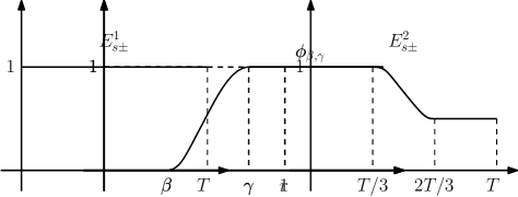
Looking to obtain a bound on of the kind that
we will choose to be such that
| (4.1) |
this leads to
Note that only for , and for . Thus
| (4.2) | ||||
5. Induction argument and convergence
We pick the super-geometric sequence to satisfy
| (5.1) |
Now we aim to establish the following estimates using an induction argument
| (5.2) |
for some , with some well-designed bounds .
5.1. Bounds on
From (3.10), (3.12), and (3.6) we find that
From the induction assumption (5.2) and the estimates on in Section 4, it follows that
| (5.3) |
By choosing
we obtain
| (5.4) |
for some constant . Since , it then follows that
Proposition 5.1.
For , there is a choice for such that
| (5.5) |
where is the -norm.
Choosing a summable sequence , the above implies that is bounded, which, combining with the estimate in Section 3.8, yields that
5.2. Bounds on
Choose so that
then we have
| (5.6) |
for some constant .
Proposition 5.2.
For , there exist suitable parameters , and such that if satisfies (5.2), then the following estimate for holds:
| (5.7) |
Proof.
We will divide the argument into the following three cases, according to the definition of .
Case 2. . In this case we have from (3.23) and (4.1) that
So we need
| (5.9) |
The above also imposes the following condition
Case 3. . Now we have
Thus for
| (5.10) |
one would obtain (5.7). As in the previous cases, the above leads to assuming
Summarizing the above, we have obtained that
| (5.12) |
Choosing sufficiently small we are able to achieve that , and hence we may take in all of the preceding estimates.
5.3. Bounds on
5.4. Bounds on
5.5. A quick summary
What we have achieved in this section is the following.
For satisfying
choose
where is as in (5.6). By choosing the two sequences , with
then the sequence of the iterative approximations enjoys the following property:
| (5.15) |
5.6. Convergence to a weak solution
From (5.15) we see that there exists a subsequence of , still denoted by , such that as ,
6. Dephasing and non-uniqueness
Sections 3–5 provide a systematic way to build weak solutions to system (1.1) from a “constant state” subsolution of the form (3.2). We would like to take advantage of the temporal phase function in the approximation iteration (3.10) to generate two distinct weak solutions and , sharing the same data at .
For this, we first define a smooth function such that
and is increasing.
Starting with the same subsolution of the form (3.2) for sufficiently small, say
| (6.1) |
as in (5.15), consider two iteration sequences and as in (3.10), where the phase functions , in the oscillatory parts and are given by
The discussion in the previous sections implies that
| (6.2) |
with being a weak solution of (1.1), for . We further choose the mollification scales to be sufficiently small such that
Proposition 6.1.
For all it holds that
| (6.3) |
where we consider when . In particular, this implies that
| (6.4) |
Proof.
Recall that now we have
We can prove that
Proposition 6.2.
Proof.
We will use an induction argument to prove (6.6) and (6.7). Consider first the case when . For any ,
and thus
From the condition (5.11) on the parameters we can choose appropriate , and the function such that , and so
Recall the definition of the localization in Section 3.3. We may choose sufficiently large such that there exists only one such that . The partition of unity further implies that at such , . Similar result holds for . Therefore we have
with
Similarly, for we have
with .
For we know that and the above becomes
Note that
Therefore
where is given in (6.5). This way, if we choose
then
Choose and sufficiently small, and hence in this region
Assume now that (6.6) and (6.7) hold for some general . When we have
where and are the right eigenvectors of , for . From (5.12) and (6.1) we see that
| (6.8) |
Similarly as before, by choosing sufficiently large, it holds that for any , , there exists a unique such that
From the definition of in Section 3.3 we know that
Therefore
where is given in (6.5). Taking we have
Using (6.8) we have
From (4.1) we know that . From (5.15) we see that . Hence
and therefore
So when , from the induction assumption,
The rest of the estimates can be obtained through the same argument. ∎
Now we can state our main non-uniqueness result of this section.
Theorem 6.1.
Proof.
7. Proof of Theorem 1.2
In this section, we study System 1.3 that substantiates our hypothesis regarding the non-uniqueness of continuous solutions within the context of a 1D system of conservation laws, and prove Theorem 1.2. Letting and , one calculates
Computing the trace and the determinant of this matrix, we find that
Hence, System (1.3) is strictly hyperbolic on , and on this set
The associated eigenvectors are
We now compute:
and so
| (7.1) |
Note that at 0, these quantities are equal to 0. Therefore, to verify of Definition 1.1, we only need to show that the curvatures are not 0.
We are able to calculate , and at . From (2.8), this would imply that if at But we can calculate that
which implies that
Therefore, System 1.3 verifies for all at 0. From Theorem 1.1, there exists such that for any ball , there exists two solutions of (1.3) in sharing the same initial value. Choosing such a ball which does not intersect the line , we see from (7.1) that, in addition, both fields are genuinely nonlinear in . This ends the proof of Theorem 1.2. Note that this system has an entropy as
in term of We can verify that
The trace of this matrix is given by for any , and its determinant is given by for any . Hence, is a convex function around . This assertion underscores the suitability of our system (1.3) as a good system.
Appendix A Calculation and estimates on the correctors
In this appendix we collect the explicit computation involved in Section 3, together with the remainder estimates.
Recall that
Using the fact that , an improved estimate can be obtained.
| (A.3) | ||||||
The remainder is defined as
| (A.6) | ||||
and
| (A.7) | ||||
The estimates of are as below.
| (A.8) | ||||||
The definition of , for , together with the corresponding estimates, are given as
| (A.9) | ||||
and
| (A.10) |
| (A.11) | ||||||
Acknowledgement
Robin Ming Chen is partially supported by the NSF grant: DMS 2205910. Alexis Vasseur is partially supported by the NSF grant: DMS 2306852. Cheng Yu is is partially supported by the Collaboration Grants for Mathematicians from Simons Foundation.
References
- [1] S. Bianchini and A. Bressan, Vanishing viscosity solutions of nonlinear hyperbolic systems, Ann. of Math. (2)161(2005), no.1, 223–342.
- [2] S. Bianchini, R. Colombo and F. Monti, systems of conservation laws with data, J. Differential Equations, 249 (2010), pp. 3466–3488.
- [3] A. Bressan, Hyperbolic systems of conservation laws. Oxford University Press, 2000.
- [4] A. Bressan and C. De Lellis, A remark on the uniqueness of solutions to hyperbolic conservation laws, Arch. Ration. Mech. Anal., 247 (2023), pp. Paper No. 106, 12.
- [5] A. Bressan and G. Guerra, Unique Solutions to Hyperbolic Conservation Laws with a Strictly Convex Entropy, J. Differential Equations 387 (2024), 432–447.
- [6] A. Bressan and M. Lewicka, A uniqueness condition for hyperbolic systems of conservation laws, Discrete Cont. Dynam. Systems 6 (2000), 673–682.
- [7] A. Bressan and P. LeFloch, Uniqueness of weak solutions to systems of conservation laws, Arch. Rational Mech. Anal. 140 (1997), no. 4, 301–317.
- [8] G. Chen, S. Krupa and A. Vasseur, Uniqueness and Weak-BV Stability for Conservation Laws, Arch. Ration. Mech. Anal. 246 (2022), no. 1, 299–332.
- [9] G. Chen, M.-J. Kang and A. Vasseur, From Navier-Stokes to BV solutions of the barotropic Euler equations, arXiv:2401.09305.
- [10] E. Chiodaroli, C. De Lellis and O. Kreml,Global ill-posedness of the isentropic system of gas dynamics, Comm. Pure Appl. Math. 68 (2015), no. 7, 1157-1190.
- [11] M. G. Crandall and P.-L. Lions, Viscosity solutions of hamilton-jacobi equations, Transactions of the American Mathematical Society, 277 (1983), pp. 1–42.
- [12] C. M. Dafermos, Hyperbolic conservation laws in continuum physics, vol. 3, Springer, 2005.
- [13] C. M. Dafermos, The second law of thermodynamics and stability, Arch. Rational Mech. Anal., 70 (1979), no. 2, pp. 167–179.
- [14] C. De Lellis and L. Székelyhidi Jr, The Euler equations as a differential inclusion, Annals of mathematics, (2009), pp. 1417–1436.
- [15] C. De Lellis and L. Székelyhidi Jr, On admissibility criteria for weak solutions of the Euler equations, Arch. Ration. Mech. Anal., 195(1):225–260, 2010.
- [16] R. J. DiPerna, Uniqueness of solutions to hyperbolic conservation laws, Indiana Univ. Math. J., 28 (1979), no. 1, pp. 137–188.
- [17] V. Giri and H. Kwon, On non-uniqueness of continuous entropy solutions to the isentropic compressible Euler equations, Arch. Ration. Mech. Anal., 245 (2022), pp. 1213–1283.
- [18] J. Glimm, Solutions in the large for nonlinear hyperbolic systems of equations, Comm. Pure Appl. Math. 18 (1965), 697-715.
- [19] J. Glimm and P. Lax, Decay of solutions of systems of nonlinear hyperbolic conservation laws, Amer. Math. Soc. Memoir 101 (1970).
- [20] W. M. Golding, S. G. Krupa and A. F. Vasseur, Sharp a-contraction estimates for small extremal shocks, Journal of Hyperbolic Differential Equations, 20 (2023), no.3, pp. 541–602.
- [21] C. J. P. Johansson and R. Tione, T5 configurations and hyperbolic systems, Communications in Contemporary Mathematics, (2023).
- [22] M.-J. Kang and A. Vasseur, Uniqueness and stability of entropy shocks to the isentropic Euler system in a class of inviscid limits from a large family of Navier–Stokes systems, Invent. Math., 224 (2021), pp.55–146.
- [23] S. G. Krupa, Finite time BV blowup for Liu-admissible solutions to P-system via computer-assisted proof, arXiv:2403.07784.
- [24] S. G. Krupa and L. Székelyhidi Jr, Nonexistence of configurations for hyperbolic systems and the Liu entropy condition, (2022).
- [25] T.-P. Liu,Nonlinear stability of shock waves for viscous conservation laws, Mem. Amer. Math. Soc. 328 (1985), v+108.
- [26] T.P. Liu and T. Yang, stability for systems of hyperbolic conservation laws, J. Amer. Math. Soc. 12 (1999), pp. 729-774.
- [27] A. Lorent and G. Peng, On the rank-1 convex hull of a set arising from a hyperbolic system of Lagrangian elasticity, Calc. Var. Partial Differential Equations, 59 (2020), pp. Paper No. 156, 36.
- [28] B. Riemann, Uber die Fortpflanzung ebener Luftwellen von endlicher Schwingungsweite, Gottingen Abh. Math. Cl. 8 (1860), pp. 43-65.
- [29] L. Tartar,Compensated compactness and applications to partial differential equations, Nonlinear analysis and mechanics: Heriot-Watt Symposium, Vol. IV, Res. Notes in Math., 39 (1979), pp. 136-212.
- [30] A. Vasseur, Recent results on hydrodynamic limits. In Handbook of differential equations: evoluationary equations. Vol. IV, Handb. Differ. Equ., pp. 323-376. Elsevier/North-Holland, Amsterdam, 2008.