EgoFlowNet: Non-Rigid Scene Flow from Point Clouds with Ego-Motion Support

Abstract

Recent weakly-supervised methods for scene flow estimation from LiDAR point clouds are limited to explicit reasoning on object-level. These methods perform multiple iterative optimizations for each rigid object, which makes them vulnerable to clustering robustness. In this paper, we propose our EgoFlowNet – a point-level scene flow estimation network trained in a weakly-supervised manner and without object-based abstraction. Our approach predicts a binary segmentation mask that implicitly drives two parallel branches for ego-motion and scene flow. Unlike previous methods, we provide both branches with all input points and carefully integrate the binary mask into the feature extraction and losses. We also use a shared cost volume with local refinement that is updated at multiple scales without explicit clustering or rigidity assumptions. On realistic KITTI scenes, we show that our EgoFlowNet performs better than state-of-the-art methods in the presence of ground surface points.

1 Introduction

Scene flow estimation is an important computer vision problem for navigation, planning, and autonomous driving systems. It provides a representation of the dynamic environment by estimating the 3D motion field relative to the observer. Until a few years ago, stereo images were used for joint disparity estimation and optical flow estimation to represent scene flow [Saxena et al.(2019)Saxena, Schuster, Wasenmüller, and Stricker, Jiang et al.(2019)Jiang, Sun, Jampani, Lv, Learned-Miller, and Kautz, Ma et al.(2019)Ma, Wang, Hu, Xiong, and Urtasun, Chen et al.(2020)Chen, Gool, Schmid, and Sminchisescu, Schuster et al.(2020)Schuster, Wasenmüller, Unger, Kuschk, and Stricker]. However, the two-view geometry used in self-driving cars has inherent limitations, such as inaccuracies in depth estimation in distant regions.

With the advent of LiDAR, many learning-based methods have been developed to estimate scene flow directly from point clouds in a fully-supervised manner [Gu et al.(2019)Gu, Wang, Wu, Lee, and Wang, Wu et al.(2020)Wu, Wang, Li, Liu, and Fuxin, Cheng and Ko(2022), Wang et al.(2022b)Wang, Hu, Liu, Zhou, Tomizuka, Zhan, and Wang, Kittenplon et al.(2021)Kittenplon, Eldar, and Raviv]. They differ from each other in their basic feature extraction framework and the way they design their cost volume. Due to the lack of annotated data on realistic sequences, some methods train their end-to-end models with self-supervised losses [Wu et al.(2020)Wu, Wang, Li, Liu, and Fuxin, Kittenplon et al.(2021)Kittenplon, Eldar, and Raviv, Mittal et al.(2020)Mittal, Okorn, and Held, Li et al.(2021b)Li, Lin, and Xie].

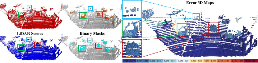
Figure 1: Our EgoFlowNet operates non-rigidly at the point-level and shows high accuracy for regions of varying local density (e.g, the red, blue, and green rectangles).

Apart from the point-wise estimation of scene flow, some methods perform better when using self-supervised losses under conditions of rigidity [Li et al.(2022)Li, Zhang, Lin, Wang, and Shen, Deng and Zakhor(2023)]. Other methods support scene flow estimation with ego-motion [Behl et al.(2019)Behl, Paschalidou, Donné, and Geiger, Tishchenko et al.(2020)Tishchenko, Lombardi, Oswald, and Pollefeys, Wang et al.(2022a)Wang, Feng, Jiang, and Wang]. All of the above methods work well on ideal conditions (e.g, no ground points, no occlusions, or with nearly direct correspondences between consecutive scenes).

A recent breakthrough has been achieved by WSLR [Gojcic et al.(2021)Gojcic, Litany, Wieser, Guibas, and Birdal], where a multi-task prediction network is designed and trained with real scenes in a weakly-supervised manner in the presence of ground points. This approach segments the scene into static parts (i.ebackground ($BG$)) and moving agents (i.eforeground ($FG$)). It then optimizes the initial estimate of ego-motion and scene flow via non-parametric object-based optimizations using explicit rigidity constraints. Towards learning-based optimization, ERC [Dong et al.(2022)Dong, Zhang, Li, Sun, and Xiong] uses the predicted segmentation mask from [Gojcic et al.(2021)Gojcic, Litany, Wieser, Guibas, and Birdal] and proposes a novel optimization method with an error-driven Gated Recurrent Unit and residual scene flow heads. These methods [Gojcic et al.(2021)Gojcic, Litany, Wieser, Guibas, and Birdal, Dong et al.(2022)Dong, Zhang, Li, Sun, and Xiong] show impressive results for more difficult scenes (e.gwith ground points, outliers, occlusions, etc). However, both methods rely on the DBSCAN clustering algorithm [Ester et al.(1996)Ester, Kriegel, Sander, Xu, et al.], which may limit their ability to work on low-density regions or under-sampled objects (e.g, distant cars or small objects). In addition, they must perform iterative optimizations for each clustered region, which negatively impacts efficiency when the scene contains a large number of clusters.

Compared to these methods, our approach is far removed from any clustering strategy and instead predicts unconstrained scene flow at the point-level. To this end, we design our multi-task network to predict a binary $FG$/$BG$ segmentation mask, which is then carefully used to estimate ego-motion and scene flow (c.f. Figure 1). Unlike object-based methods, we feed the ego-motion and scene flow branches with all input points, integrate our predicted mask into both branches and combine everything with point-based coarse-to-fine refinement to obtain accurate scene flow. For robust estimation in both branches, we also develop a hybrid feature extraction to provide both branches with well-suited features.

Our contributions are summarized as follows:

• We propose EgoFlowNet – a multi-task neural network architecture to estimate scene flow directly from raw point clouds that jointly estimates binary segmentation masks, ego-motion, and scene flow.

• We propose a hybrid feature extraction along with a hybrid warping layer and integrate the binary masks to obtain robust scene flow.

• We work with a point-level refinement of the scene flow, which is free of explicit clustering mechanisms or rigidity assumptions for dynamic objects.

• On difficult real LiDAR scenes (i.e, with ground points, occlusions, and outliers), we show that our proposed approach outperforms recent clustering-based methods.

2 Related Work

3D scene flow was first introduced in the image domain using RGB-D [Jaimez et al.(2015)Jaimez, Souiai, Gonzalez-Jimenez, and Cremers, Jaimez et al.(2017)Jaimez, Kerl, Gonzalez-Jimenez, and Cremers, Qiao et al.(2018)Qiao, Gao, Lai, Zhang, Yuan, and Xia, Shao et al.(2018)Shao, Shah, Dwaracherla, and Bohg] for indoor scenarios and stereo images [Vogel et al.(2015)Vogel, Schindler, and Roth, Ilg et al.(2018)Ilg, Saikia, Keuper, and Brox, Jiang et al.(2019)Jiang, Sun, Jampani, Lv, Learned-Miller, and Kautz, Ma et al.(2019)Ma, Wang, Hu, Xiong, and Urtasun, Chen et al.(2020)Chen, Gool, Schmid, and Sminchisescu, Schuster et al.(2020)Schuster, Wasenmüller, Unger, Kuschk, and Stricker, Teed and Deng(2021)] for outdoor scenarios. However, learning scene flow directly from point clouds without relying on RGB images opens up a wide field of research [Wang et al.(2018)Wang, Suo, Ma, Pokrovsky, and Urtasun, Liu et al.(2019)Liu, Qi, and Guibas, Gu et al.(2019)Gu, Wang, Wu, Lee, and Wang, Wu et al.(2020)Wu, Wang, Li, Liu, and Fuxin, Puy et al.(2020)Puy, Boulch, and Marlet, Wei et al.(2021)Wei, Wang, Rao, Lu, and Zhou, Kittenplon et al.(2021)Kittenplon, Eldar, and Raviv, Li et al.(2021a)Li, Lin, He, Liu, and Shen, Wang et al.(2021)Wang, Wu, Liu, and Wang, Gojcic et al.(2021)Gojcic, Litany, Wieser, Guibas, and Birdal, Gu et al.(2022)Gu, Tang, Yuan, Dai, Zhu, and Tan, Cheng and Ko(2022), Dong et al.(2022)Dong, Zhang, Li, Sun, and Xiong, Deng and Zakhor(2023)].

GRU-based Scene Flow from Point Cloud: The Gated Recurrent Unit (GRU) [Cho et al.(2014)Cho, Van Merriënboer, Gulcehre, Bahdanau, Bougares, Schwenk, and Bengio] is used to iteratively refine the global cost volume to provide an accurate estimate of the scene flow [Teed and Deng(2021)]. FlowStep3D [Kittenplon et al.(2021)Kittenplon, Eldar, and Raviv] updates the cost volume locally using GRU with multiple reconstructions and iterative point cloud alignment. To encode a large correspondence set within the cost volume, PV-RAFT [Wei et al.(2021)Wei, Wang, Rao, Lu, and Zhou] combines a voxel representation with a point-wise cost volume. A point-wise optimization combined with a recurrent network regularization is proposed by RCP [Gu et al.(2022)Gu, Tang, Yuan, Dai, Zhu, and Tan]. Our EgoFlowNet avoids strict iterative updates and works from coarse-to-fine, driven by a binary segmentation mask and jointly estimates scene flow and the ego-motion.

Hierarchical Scene Flow from Point Cloud: FlowNet3D [Liu et al.(2019)Liu, Qi, and Guibas] is the first work to introduce a cost volume layer from a point cloud with hierarchical refinement. However, it is limited to a single cost volume layer. To overcome this limitation, HPLFlowNet [Gu et al.(2019)Gu, Wang, Wu, Lee, and Wang] introduces multi-scale correlation layers by projecting points into a permutohedral grid [Su et al.(2018)Su, Jampani, Sun, Maji, Kalogerakis, Yang, and Kautz]. Moving away from the grid representation, PointPWC-Net [Wu et al.(2020)Wu, Wang, Li, Liu, and Fuxin] improves the direct estimation of scene flow from raw point clouds by constructing cost volumes at a range of scales from coarse-to-fine. Following the hierarchical point-based designs, intensive improvements are proposed in the development of cost volume using dual attentions as in [Wang et al.(2021)Wang, Wu, Liu, and Wang, Wang et al.(2022c)Wang, Hu, Wu, and Wang, Wang et al.(2022b)Wang, Hu, Liu, Zhou, Tomizuka, Zhan, and Wang, Battrawy et al.(2022)Battrawy, Schuster, Mahani, and Stricker]. Our network is basically hierarchical, but integrates further multi-task estimates of ego-motion and segmentation. It operates in challenging outdoor scenes with typical occlusions and in dense scenes with ground points.

Scene Flow from Point Cloud with Constraints: Axiomatic concepts of rigidity assumptions are explored in [Deng and Zakhor(2023), Li et al.(2022)Li, Zhang, Lin, Wang, and Shen] along with cluster-based or object-level optimization. However, the above methods are not well explored with typical outdoor scenes in the presence of ground surface points. More recently, WSLR [Gojcic et al.(2021)Gojcic, Litany, Wieser, Guibas, and Birdal] has proposed pioneering weakly-supervised learning along with non-parametric optimization, and ERC [Dong et al.(2022)Dong, Zhang, Li, Sun, and Xiong] extends this to learning-based optimization. Both work well on challenging outdoor scenes where ground points are present. However, both require multiple optimization steps and work under object-level constraints using DBSCAN clustering [Ester et al.(1996)Ester, Kriegel, Sander, Xu, et al.]. Chodosh et al [Chodosh et al.(2023)Chodosh, Ramanan, and Lucey] is a very recent conventional and cluster-based method that works by test time optimization using ICP [Besl and McKay(1992), Segal et al.(2009)Segal, Haehnel, and Thrun] and RANSAC to achieve appropriate piece-wise rigidity. In contrast to the above methods, we do not use clustering algorithms and work with point-level optimization, which allows us to estimate non-rigid motion and is more accurate and robust than state-of-the-art methods.

3 Network Design

Our EgoFlowNet estimates scene flow as translational vectors from two consecutive frames of point clouds, with no assumptions about object rigidity. Given Cartesian 3D point cloud frames $P$ and $Q$ at timestamps $t$ and $t+1$, our goal is to estimate point-wise 3D flow vectors $\hat{S}$ for each point within $P$. Our network is designed to combine segmentation, ego-motion, and scene flow tasks at four scales $\{L\}^{3}_{k=0}$, where $l_{0}$ is the full resolution of $P$ and $Q$. An illustration of our hierarchical modules of our feature extraction, cost volume, ego-motion and scene flow is given in Figure 2, where the right part of the figure illustrates a single layer or scale $l_{k}$ for each of these modules. The following sections describe the components of each module in detail.

3.1 Feature Extraction

Our feature extraction module consists of two networks: The first one is an encoder-decoder module, while the second one consists only of a context encoder. The backbone of our feature extraction is inspired by RandLA-Net [Hu et al.(2020)Hu, Yang, Xie, Rosa, Guo, Wang, Trigoni, and Markham].

Encoder Module: Each scale in the encoder module essentially consists of two layers, where Local-Feature-Aggregation (LFA) is applied to aggregate the features at the $l_{k}$ scale, followed by a Down-Sampling (DS) layer to aggregate the features from the $l_{k}$ level to $l_{k+1}$, resulting in a simultaneous decrease in resolution. The backbone of the LFA is inspired by RandLA-Net [Hu et al.(2020)Hu, Yang, Xie, Rosa, Guo, Wang, Trigoni, and Markham], which uses attentive pooling based on self-attention as in [Yang et al.(2020)Yang, Wang, Markham, and Trigoni, Zhang and Xiao(2019)]. At all scales, we search for 16 neighbors in Euclidean space using K-Nearest-Neighbors (KNNs), then their weighted features are summed based on attentive pooling. The DS layer samples the points based on Farthest-Point-Sampling (FPS) to the defined resolution $l_{k+1}$, and aggregates $16$ nearest neighbors in the higher resolution $l_{k}$ for each selected sample simply by using Max-Pooling.

Decoder Module: The decoder module of the hourglass network consists of ${\{L\}}^{3}_{k=0}$ layers for extracting the features up to the full (input) resolution $l_{0}$ of $P$ and $Q$, respectively. To up-sample from the $l_{k+1}$ level to $l_{k}$, we simply assign the one nearest neighbor for each point of the higher resolution to the lower one, followed by a simple Multi-Layer Perceptron (MLP). To increase the quality of the features in the encoder-decoder network, lateral connections are added to each layer.

Segmentation Features: The encoder-decoder of the first network extracts the features $F^{P}_{s,0}$ and $F^{Q}_{s,0}$ at the input resolution, which are used to predict the binary segmentation masks ($M^{P}_{fg}$ and $M^{Q}_{fg}$) and/or ($M^{P}_{bg}$ and $M^{Q}_{bg}$) for $P$ and $Q$, respectively.

Hybrid Features: The encoder module of the first network and the context network compute the features ($F^{P}_{encoder,k}$, $F^{Q}_{encoder,k}$) and ($F^{P}_{context,l}$, $F^{Q}_{context,k}$), at each scale level $l_{k}$. The encoder modules down-sample the input to the resolutions $l_{1}=2048,l_{2}=512,l_{3}=128$ with feature dimensions $C_{0}=32,C_{1}=128,C_{2}=256,C_{3}=512$. The output features of the two encoders at each scale level $l_{k}$ are merged using the predicted and down-sampled segmentation masks $M_{fg,k}$ as follows:

$$HF_{k}=M_{fg,k}\cdot{F_{context,k}}+(1-M_{fg,k})\cdot{\perp{(F_{encoder,k})}},$$ (1)

where $M_{fg,k}$ refers to the binary mask of foreground points, ($1-M_{fg,k}$) refers to the background mask (i.e, $M_{bg,k}$) and $\perp$ is an operator that sets the gradient of the operand to zero, $\triangledown{(x)}=0$ (i.e, stop gradient). Since the number of background points ($BG$) within a scene, including the ground points, is usually much higher than the number of foreground points ($FG$), using the stop gradient eliminates the negative effect of the ego-motion branch on the segmentation head and the scene flow branch. By merging the context encoders, the features of the $FG$ points can be enhanced to provide an accurate estimate of scene flow for these points. We apply Eq. 1 at each scale level $l_{k}$ using $M^{P}_{fg,k}$ and $M^{Q}_{fg,k}$, resulting in $HF^{P}_{k}$ and $HF^{Q}_{k}$ for $P$ and $Q$, respectively, which are then used for the shared cost volume.

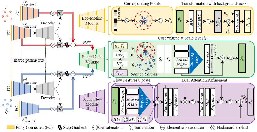
Figure 2: Our EgoFlowNet architecture predicts a binary segmentation masks ($M^{P}_{fg}$ and $M^{Q}_{fg}$) for foreground points ($FG$) and ($M^{P}_{bg}$ and $M^{Q}_{bg}$) for background points ($BG$). We use the binary mask to jointly estimate ego-motion and scene flow at the point-level. For this, we extract hybrid features ($HF^{P}$ and $HF^{Q}$) and hierarchically refine our point-wise scene flow.

3.2 Segmentation Head

We apply three layers of Multi-Layer Perceptions (MLPs) with 64, 32 and 1 output channels to the computed segmentation features $F^{P}_{s,0}$ and $F^{Q}_{s,0}$. The output of the last layer provides the segmentation probabilities at full (input) resolution layer $l_{0}$, allowing us to define the binary segmentation masks $M^{P}_{fg}$ and $M^{Q}_{fg}$ for $P$ and $Q$, respectively.

3.3 Shared Cost Volume

We learn the geometric and feature correlations based on the hybrid features $HF^{P}_{k}$ and $HF^{Q}_{k}$ (c.f. Eq. 1).

Searching for Correspondences: As a first step, we need to find the correlation set in $Q_{k}$ for each point in $P_{k}$. Since finding correlations based on Euclidean space may not be sufficient to capture distant correspondences, we use the feature space to find the correspondences at the coarsest scale $l_{3}$. This provides a high quality initial estimate of the scene flow $\hat{S}_{3}$ and a high quality initial estimate of the ego-motion parameters represented by the rotation $\hat{R}_{3}$ and translation $\hat{t}_{3}$ components. For the scene flow, when searching for correspondences in feature space, the distant matches on the upper scales are approximated by our hybrid warping layer so that the warped point cloud $\widetilde{P}_{k}$ is close to its match in $Q_{k}$. With this initialization, it becomes worthwhile to search for the closest $16$ matches in Euclidean space for the upper scales $\{L\}^{2}_{k=0}$.

After grouping the correspondence set with its geometric features ${\{q_{j,k}\}}^{16}_{j=1}$ and hybrid features ${\{{hf}^{q}_{j,k}\}}^{16}_{j=1}$, we compute the differences to the point $P_{k}$ and its hybrid feature ${hf}^{P}_{i,k}$, respectively. This yields the geometric and feature differences $\widetilde{G}_{k}$ and $\widetilde{F}_{k}$, which are then concatenated. We apply Max-Pooling along the feature dimension to compute attentive weights similar to HRegNet [Lu et al.(2021)Lu, Chen, Liu, Zhang, Qu, Liu, and Gu]. The geometric and feature differences are then smoothly weighted by the attentional weights and summed to obtain ${\hat{F}}_{k}$.

Hybrid Warping Layer: Our hybrid warping layer (${HW}_{k}$) is jointly driven by the ego-motion, the scene flow, and the predicted segmentation $M^{P}_{fg,k}$ of frame $P_{k}$. After obtaining the initial ego-motion and the initial scene flow at the coarse scale $l_{3}$, we apply hybrid warping to refine the estimate at the upper scales $\{L\}^{2}_{k=0}$. Fo this purpose, we use the the corresponding binary masks ($M^{P}_{fg,k}$ and $M^{P}_{bg,k}$), the up-sampled scene flow ${\hat{S}}_{k}$ from the coarser scale through a simple Up-Sampling layer (${US}_{k}$), and the ego-motion transformation to warp the points in $P_{k}$ towards the target $Q_{k}$ and obtain ${\widetilde{P}}_{k}$. For all upper scales, we apply the following equation:

$${\widetilde{P}}_{k}=M_{fg,k}\cdot{(P_{k}+{\hat{S}}_{k}})+(M_{bg,k}\cdot{((\hat{R}_{k}P^{T}_{k})^{T}+\hat{t}_{k})}$$ (2)

3.4 Ego-Motion branch

We compute point correspondences and apply the Kabsch algorithm [Kabsch(1976)] to estimate the ego-motion parameters $\hat{R}_{k}$ and $\hat{t}_{k}$.

Corresponding Points: Inspired by HRegNet [Lu et al.(2021)Lu, Chen, Liu, Zhang, Qu, Liu, and Gu], after obtaining the correspondence set ${\{q_{j,k}\}}^{16}_{j=1}$ for each point in $Q_{k}$ as described in the cost volume, we multiply the computed attentive weights with them and sum over the nearest neighbors to obtain the corresponding points $\hat{P}_{k}$.

Optimal Transformation: Multi-Layer Perceptrons (MLPs) are applied to the cost volume output ${\hat{F}}_{k}$, followed by a Sigmoid function to obtain confidence values inspired by [Lu et al.(2021)Lu, Chen, Liu, Zhang, Qu, Liu, and Gu, Gojcic et al.(2021)Gojcic, Litany, Wieser, Guibas, and Birdal, Dong et al.(2022)Dong, Zhang, Li, Sun, and Xiong]. However, unlike previous approaches [Dong et al.(2022)Dong, Zhang, Li, Sun, and Xiong, Gojcic et al.(2021)Gojcic, Litany, Wieser, Guibas, and Birdal], we do not filter out the ($FG$) points to feed the ego-motion branch with only ($BG$) points. Instead, we feed this branch with all points and multiply the confidence values by $M^{P}_{bg,k}$, to refine the corresponding points $\hat{P}_{k}$ so that the transformation matrix can be computed according to [Kabsch(1976)] to obtain $\hat{R}_{k}$ and $\hat{t}_{k}$.

3.5 Scene Flow branch

Across all scales, our scene flow branch consists of three refinement stages and four scene flow predictors with simple nearest-neighbor Up-Sampling (US). The total number of layers with attention-based refinement is inspired by RMS-FlowNet [Battrawy et al.(2022)Battrawy, Schuster, Mahani, and Stricker], which is designed to estimate scene flow only, but we add three feature updating units.

Feature Updates: With the obtained cost volume features ${\hat{F}}_{k}$, we search for the 16 nearest neighbors in the feature space, group them and then apply MLPs followed by Max-Pooling. This helps to capture similar features and implicitly extends features to semantic objects as inspired by DGCNN [Wang et al.(2019)Wang, Sun, Liu, Sarma, Bronstein, and Solomon].

Dual Attention Refinement: We concatenate the updated features ${\hat{F}}_{k}$ with $HF^{P}_{k}$, $\hat{SF}_{k}$ and $\hat{S}_{k}$, where the latter two components are the scene flow features and the scene flow, respectively. Both are initialized to zero in the coarse layer $l_{3}$ and are only used in the upper scales ${\{L\}}^{2}_{k=1}$. We use the defined nearest neighbors ($16$) in Euclidean space to group the concatenated features and we apply dual attentions to refine the corresponding features as performed in [Battrawy et al.(2022)Battrawy, Schuster, Mahani, and Stricker].

Scene Flow Predictor: Our EgoFlowNet predicts scene flow at multiple scales, inspired by [Wu et al.(2020)Wu, Wang, Li, Liu, and Fuxin, Battrawy et al.(2022)Battrawy, Schuster, Mahani, and Stricker]. The scene flow estimation head takes the resulting scene flow features at each scale $\hat{SF}_{k}$ and applies three layers of MLPs with 64, 32 and 3 output channels. Then, the estimated scene flow $\hat{S}_{k}$ and the features from the attention-based refinement are up-sampled to the next higher scale using a simple KNN search.

3.6 Scene Flow of $\mathbf{BG}$ Points

At the input point resolution $l_{0}$, we compute the scene flow of the background $BG$ from the predicted rotation and translation (i.e, $\hat{R}_{0}$ and $\hat{t}_{0}$) of the ego-motion branch. We use the binary segmentation mask $M^{P}_{bg}$ to merge the scene flow of the $BG$ points with the output of the scene flow $\hat{S}_{0}$ obtained from the scene flow branch.

3.7 Loss Function

To guide the training of segmentation, ego-motion, and scene flow, we combine three losses:

$$\mathcal{L}_{total}=\mathcal{L}_{seg}+\mathcal{L}_{ego}+\mathcal{L}_{sf},$$ (3)

Segmentation Loss: We use the Weighted Binary Cross-Entropy loss to overcome the severe imbalance of $FG$ and $BG$ classes as follows:

$$\mathcal{L}_{seg}=-\frac{1}{N}\sum_{i=1}^{N}\gamma\cdot{y_{i}}\cdot{log(\sigma{(p(y_{i}))})}+(1-y_{i})\cdot{log(1-\sigma{(p(y_{i}))})},$$ (4)

where $i$ is the index in $P$ or $Q$, $y_{i}$ is the ground truth label, $p(y_{i})$ is the probability of the predictions and $\gamma$ is the $FG$ class weight, which is set to 20.

Ego-Motion Loss: Inspired by [Lu et al.(2021)Lu, Chen, Liu, Zhang, Qu, Liu, and Gu], the ego-motion loss is computed hierarchically. Given a four-scale estimate of the transformation parameters $\hat{R}_{k}$ and $\hat{t}_{k}$ and the ground truth $R$ and $t$, we compute the final ego-motion loss as follows:

$$\mathcal{L}_{ego}=\frac{1}{4}\sum_{k=0}^{3}\beta{\|{\hat{R}}^{T}_{k}R-I\|}_{2}+{\|{\hat{t}}_{k}-t\|}_{2}$$ (5)

where ${\|.\|}_{2}$ denotes the $L_{2}$-norm and $\beta$ is set to $1.8$.

Scene Flow Losses: To train the scene flow branch, we apply a bidirectional Chamfer loss $\mathcal{L}_{cd,k}$ and Smoothness loss $\mathcal{L}_{sm,k}$ per scale, both driven by $M^{P}_{fg,k}$ and $M^{Q}_{fg,k}$ as follows:

$$\mathcal{L}_{cd,k}=\sum_{\tilde{p_{k}}\in{\tilde{P}}_{k}}m^{P}_{fg,k}\cdot{\underset{q_{k}\in Q_{k}}{min}{\|{\tilde{p}}_{k}-q_{k}\|}_{2}}+\sum_{q_{k}\in Q_{k}}m^{Q}_{fg,k}\cdot{\underset{{\tilde{p}}_{k}\in{\tilde{P}}_{k}}{min}{\|{\tilde{p}}_{k}-q_{k}\|}_{2}}$$ (6)

$$\mathcal{L}_{sm,k}=\sum_{p^{i}_{k}\in P_{k}}m^{P}_{fg,k}\cdot{\frac{1}{N_{k}(p^{i}_{k})}\sum_{p^{j}_{k}\in N_{k}(p^{i}_{k})}{\|{\hat{S}_{k}}(p^{j}_{k})-\hat{S}_{k}(p^{i}_{k})\|}_{1}}$$ (7)

where ${\|.\|}_{1}$ denotes the $L_{1}$-norm, and the number of neighborhood points are $N_{0}=16,N_{1}=12,N_{2}=8,N_{3}=4$. Both losses are then combined as follows:

$$\mathcal{L}_{sf}=\sum_{k=0}^{3}{\alpha}_{k}(\mathcal{L}_{cd,k}+\mathcal{L}_{sm,k}),$$ (8)

and the weights per scale are ${\alpha}_{0}=0.02,{\alpha}_{1}=0.04,{\alpha}_{2}=0.08,{\alpha}_{3}=0.16$.

4 Experiments

First, we give a brief description of the data sets and metrics used for evaluation. We also demonstrate the accuracy of the method in comparison to state-of-the-art methods. Finally, there is a verification of our design choices.

4.1 Evaluation Metrics

Let $\hat{S}$ denotes the predicted scene flow, and $S$ denotes the ground truth scene flow. The evaluation metrics for the 3D motion are averaged over all points and computed as follows:

• EPE3D [m]: The 3D end-point error computed in meters as ${\|\hat{S}-S\|}_{2}$.

• Acc3DS [%]: The strict 3D accuracy which is the ratio of points whose EPE3D $<0.05~{}m$ or relative error $<5\%$.

• Acc3DR [%]: The relaxed 3D accuracy which is the ratio of points whose EPE3D $<0.1~{}m$ or relative error $<10\%$.

• Out3D [%]: The ratio of outliers whose EPE3D $>0.3~{}m$ or relative error $>10\%$.

To evaluate the predicted ego-motion parameters (i.e, $\hat{R}$ and $\hat{t}$), compared to the ground truth ($R$ and $t$), respectively, we report the following metrics averaged over all the consecutive scenes:

• RAE [$\mathbf{\degree}$]: The relative angular error computed in degrees as: $\arccos(\mathrm{Tr}(\hat{R}^{T}R-1)/2)$.

• RTE [m]: The relative translation error computed in meters as ${\|\hat{t}-t\|}_{2}$.

4.2 Data Sets and Preprocessing

As with all related methods, the point clouds generated from the following data sets are randomly sub-sampled to be evaluated at a defined resolution (e.g, 8192 points) and are shuffled in a random order to resolve possible correlations between consecutive point clouds. We evaluate all of the methods in the different versions of KITTI that are described below. All data include ground surface points.

semKITTI [Behley et al.(2019)Behley, Garbade, Milioto, Quenzel, Behnke, Stachniss, and Gall]: It contains semantic labels of point clouds and ego-motion ground truth, including many sequences of real-world autonomous driving scenes. WSLR [Gojcic et al.(2021)Gojcic, Litany, Wieser, Guibas, and Birdal] has created a preprocessed version of this data set, including large sequences for training and a test split.

stereoKITTI [Menze and Geiger(2015)]: This is a real scene flow data set with scene flow labels. As with most LiDAR-based methods, it is preprocessed using HPLFlowNet [Gu et al.(2019)Gu, Wang, Wu, Lee, and Wang]. This processing creates direct correlations across the consecutive scenes, and exhibits non-uniform point cloud density.

lidarKITTI [Geiger et al.(2012)Geiger, Lenz, and Urtasun]: Unlike $\mathrm{stereoKITTI}$, the consecutive point clouds in this data set are not in direct correspondence and some points have typical occlusions. The scene flow vectors of the ground truth are obtained by mapping the points to the corresponding pixels in the $\mathrm{stereoKITTI}$ data set. The point clouds have a non-uniform density that mimics the sampling pattern of a typical LiDAR scan. We use exactly the preprocessed and published data from WSLR [Gojcic et al.(2021)Gojcic, Litany, Wieser, Guibas, and Birdal].

4.3 Comparison to State-of-the-Art

To demonstrate the accuracy of our model, we compare our segmentation, ego-motion estimation, and scene flow estimation with state-of-the-art methods.

Segmentation and Ego-Motion:

Table 1: The segmentation accuracy of our EgoFlowNet generalizes better to $\mathrm{lidarKITTI}$ and shows better results for ego-motion estimation (i.e, $\mathrm{RAE}$ and $\mathrm{RTE}$) on $\mathrm{semKITTI}$.

Method	$\mathbf{semKITTI}$ [Behley et al.(2019)Behley, Garbade, Milioto, Quenzel, Behnke, Stachniss, and Gall]						$\mathbf{lidarKITTI}$ [Geiger et al.(2012)Geiger, Lenz, and Urtasun]
	prec. FG $\mathbf{\uparrow}$	rec. FG $\mathbf{\uparrow}$	prec. BG $\mathbf{\uparrow}$	rec. BG $\mathbf{\uparrow}$	RAE $\mathbf{\downarrow}$	RTE $\mathbf{\downarrow}$	prec. FG $\mathbf{\uparrow}$	rec. FG $\mathbf{\uparrow}$	prec. BG $\mathbf{\uparrow}$	rec. BG $\mathbf{\uparrow}$
	[%]	[%]	[%]	[%]	[$\degree$]	[m]	[%]	[%]	[%]	[%]
WSLR [Gojcic et al.(2021)Gojcic, Litany, Wieser, Guibas, and Birdal]	0.950	0.892	0.991	0.996	0.116	0.029	0.734	0.855	0.991	0.980
Ours	0.898	0.922	0.997	0.996	0.097	0.024	0.797	0.887	0.992	0.975

Table 2: We outperform point-wise models that are fully supervised and methods that optimize for rigid motion at the object-level [Gojcic et al.(2021)Gojcic, Litany, Wieser, Guibas, and Birdal, Dong et al.(2022)Dong, Zhang, Li, Sun, and Xiong, Chodosh et al.(2023)Chodosh, Ramanan, and Lucey].

Data Set	Method	Sup.	Rigid.	$\mathbf{stereoKITTI}$ [Menze and Geiger(2015)]				$\mathbf{lidarKITTI}$ [Geiger et al.(2012)Geiger, Lenz, and Urtasun]
				EPE3D $\mathbf{\downarrow}$	Out3D $\mathbf{\downarrow}$	Acc3DS $\mathbf{\uparrow}$	Acc3DR $\mathbf{\uparrow}$	EPE3D $\mathbf{\downarrow}$	Out3D $\mathbf{\downarrow}$	Acc3DS $\mathbf{\uparrow}$	Acc3DR $\mathbf{\uparrow}$
				[m]	[%]	[%]	[%]	[m]	[%]	[%]	[%]
$\mathbf{FT3D_{s}}$ [Mayer et al.(2016)Mayer, Ilg, Hausser, Fischer, Cremers, Dosovitskiy, and Brox]	PointPWC-Net [Wu et al.(2020)Wu, Wang, Li, Liu, and Fuxin]	full	✗	0.204	0.645	0.292	0.556	0.710	0.932	0.114	0.219
	FlowStep3D [Kittenplon et al.(2021)Kittenplon, Eldar, and Raviv]	full	✗	0.109	0.391	0.577	0.765	0.797	0.929	0.087	0.184
	RMS-FlowNet [Battrawy et al.(2022)Battrawy, Schuster, Mahani, and Stricker]	full	✗	0.199	0.547	0.391	0.618	0.652	0.920	0.120	0.233
	WM3D [Wang et al.(2022b)Wang, Hu, Liu, Zhou, Tomizuka, Zhan, and Wang]	full	✗	0.119	0.487	0.488	0.721	0.646	0.928	0.165	0.270
	Bi-PointFlowNet [Cheng and Ko(2022)]	full	✗	0.135	0.439	0.578	0.760	0.686	0.905	0.179	0.268
	Chodosh et al [Chodosh et al.(2023)Chodosh, Ramanan, and Lucey]	None	✓	-	-	-	-	0.061	-	0.917	0.962
$\mathbf{semKITTI}$ [Behley et al.(2019)Behley, Garbade, Milioto, Quenzel, Behnke, Stachniss, and Gall]	WSLR [Gojcic et al.(2021)Gojcic, Litany, Wieser, Guibas, and Birdal]	Weak	✓	0.068	0.263	0.836	0.897	0.080	0.369	0.742	0.850
	ERC [Dong et al.(2022)Dong, Zhang, Li, Sun, and Xiong]	Weak	✓	0.053	0.269	0.858	0.917	0.065	0.290	0.857	0.940
	Ours	Weak	✗	0.039	0.212	0.922	0.966	0.049	0.267	0.918	0.964

We compare the predicted mask and ego-motion estimates of our EgoFlowNet with the pioneering work of WSLR [Gojcic et al.(2021)Gojcic, Litany, Wieser, Guibas, and Birdal], which is the first to jointly predict binary segmentation, ego-motion, and scene flow for point clouds in a single network. The comparison is shown in Table 1. The results shown by WSLR [Gojcic et al.(2021)Gojcic, Litany, Wieser, Guibas, and Birdal] are the best optimized results presented in their paper, obtained by pre-training on FlyingThings3D [Mayer et al.(2016)Mayer, Ilg, Hausser, Fischer, Cremers, Dosovitskiy, and Brox] and subsequent further training on $\mathrm{semKITTI}$ [Behley et al.(2019)Behley, Garbade, Milioto, Quenzel, Behnke, Stachniss, and Gall]. With the exception of $FG$ precision, our model trained from scratch on the same training split of $\mathrm{semKITTI}$ outperforms WSLR on all other segmentation metrics. Since we predict point-wise scene flow for the $FG$, errors in the segmentation have less impact compared to other methods that predict rigid object motion. That said, our segmentation generalizes better to $\mathrm{lidarKITTI}$ and outperforms WSLR in the $FG$ category. In addition, our ego-motion estimation (i.e, rotation $\mathrm{RAE}$, and translation $\mathrm{RTE}$ errors ) on $\mathrm{semKITTI}$ surpasses that of WSLR [Gojcic et al.(2021)Gojcic, Litany, Wieser, Guibas, and Birdal].

Scene Flow: The ultimate goal of our model is to predict the scene flow for each input point in the scene with respect to point cloud $P$. To this end, we evaluate our final scene flow estimate against point-wise methods [Wu et al.(2020)Wu, Wang, Li, Liu, and Fuxin, Kittenplon et al.(2021)Kittenplon, Eldar, and Raviv, Battrawy et al.(2022)Battrawy, Schuster, Mahani, and Stricker, Wang et al.(2022b)Wang, Hu, Liu, Zhou, Tomizuka, Zhan, and Wang, Cheng and Ko(2022)], which are state-of-the-art methods that perform best on $\mathrm{stereoKITTI}$ when ground points are omitted. However, the accuracy of these methods is severely limited in the presence of ground points on $\mathrm{stereoKITTI}$ and even worse on $\mathrm{lidarKITTI}$, a data set that resembles real LiDAR scenes with occlusions and no direct correspondences between successive LiDAR scans. Our point-based scene flow is comparable to the latest conventional method [Chodosh et al.(2023)Chodosh, Ramanan, and Lucey] on $\mathrm{lidarKITTI}$, which integrates the ego-motion and rigidity assumptions into the scene flow estimation, but our method performs significantly better with respect to EPE3D. We also outperform the object-based weakly supervised methods WSLR [Gojcic et al.(2021)Gojcic, Litany, Wieser, Guibas, and Birdal] and ERC [Dong et al.(2022)Dong, Zhang, Li, Sun, and Xiong] on both KITTI versions in all metrics (c.f. Table 2). We also visualize our qualitative results on $\mathrm{lidarKITTI}$ in Figure 3. Further qualitative results can be found in the supplementary material.

Efficiency: Our model contains about 16 million parameters. For $8192$ input points, it requires 11 GFLOPs, which takes an average of $140ms$ for a pair of point clouds on a single NVIDIA Titan V.

	Example 1	Example 2	Example 3
Scene
$M^{P}_{fg}$
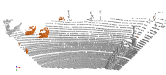
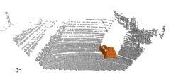
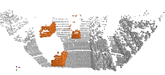
Error Map

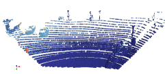
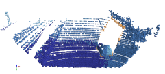
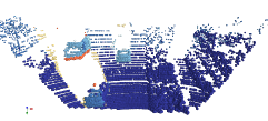
Figure 3: Three examples from $\mathrm{lidarKITTI}$ [Geiger et al.(2012)Geiger, Lenz, and Urtasun] show the qualitative results of our EgoFlowNet. For visual enhancement only, we show the RGB images of each scene. We visualize the predicted binary mask, where $BG$ and $FG$ points are encoded by gray and orange colors, respectively. The error map for each scene (third row) shows the end-point error in meters and is colored according to the map shown in the last row. Our EgoFlowNet shows low errors (dark blue) over a wide area in each scene, including $FG$ and $BG$ points.

4.4 Ablation Study

We conduct several experiments by training on $\mathrm{semKITTI}$ and evaluating on $\mathrm{lidarKITTI}$ to verify our design decisions. To do this, we evaluate $FG$ and $BG$ points separately in $\mathrm{EPE3D_{fg}}$ and $\mathrm{EPE3D_{bg}}$, respectively. We build our baseline design by computing our features from the encoder of the first feature extraction network ($F_{encoder}$), so that no context encoder module and hybrid features are applied, and we do not consider binary masks for any of our network branches (i.e, ego-motion and scene flow) and our warping layer is computed based on the scene flow branch only. Then, we check the basic estimates of our model by applying only the proposed losses (c.f. Eq. 3), as shown in the $1^{st}$ row in Table 3. In the $2^{nd}$ row, we see the positive influence of integrating the predicted background mask $\mathrm{M^{P}_{bg}}$ into the ego-motion branch. In the $3^{rd}$ row, we apply our hybrid warping layer as in Eq. 2, which further improves the results. Adding scene flow feature updating and dual attention refinement significantly improves the results for all metrics, as can be clearly seen in rows $4^{th}$ and $5^{th}$. Without the stop gradient in Eq. 1, the results are the same as after using refinements, but applying it shows an improvement in $\mathrm{EPE3D_{fg}}$ and consequently in all other metrics. We provide further experiments in the supplementary material.

Table 3: We investigate the contribution of each component in our design on $\mathrm{lidarKITTI}$ [Geiger et al.(2012)Geiger, Lenz, and Urtasun].

$\mathbf{M^{P}_{bg}}$	Hyprid	Feature	Attention	Hybrid	Hybrid	$\mathbf{EPE3D}~{}\downarrow$	$\mathbf{EPE3D_{fg}}~{}\downarrow$	$\mathbf{EPE3D_{bg}}~{}\downarrow$	Acc3DR $\uparrow$
	Warping	Update	Refinement	Features	Features $\perp{}$	[m]	[m]	[m]	[%]
✗	✗	✗	✗	✗	✗	0.168	0.375	0.154	0.689
✓	✗	✗	✗	✗	✗	0.139	0.363	0.119	0.808
✓	✓	✗	✗	✗	✗	0.085	0.335	0.065	0.871
✓	✓	✓	✗	✗	✗	0.067	0.326	0.048	0.931
✓	✓	✓	✓	✗	✗	0.053	0.287	0.035	0.952
✓	✓	✓	✓	✓	✗	0.053	0.282	0.036	0.957
✓	✓	✓	✓	✓	✓	0.049	0.267	0.033	0.964

5 Conclusion

We propose EgoFlowNet, which predicts binary segmentation masks for dynamic and static LiDAR-based scenes and jointly estimates hierarchical ego-motion and scene flow. Our method works by estimating scene flow at the point-level rather than optimizing it at the object level. Our network is free of any clustering and uses point-level refinement, which produces better results than competing methods and allows for non-rigid object motions. Our approach outperforms recent approaches that rely on the object-level and shows robust accuracy in the presence of ground points.

Acknowledgment

This work was partially funded by the Federal Ministry of Education and Research Germany under the project DECODE (01IW21001) and partially in the funding program Photonics Research Germany under the project FUMOS (13N16302).

SUPPLEMENTARY

In our supplementary material, we explain details of implementation, training and augmentation and we perform further ablation studies to validate our design choices. We then add another comparison with a newer method that works under the assumption of rigidity. Finally, we discuss the possible shortcomings of our approach and show more qualitative results.

I Implementation, Training and Augmentation

Following related approaches [Gojcic et al.(2021)Gojcic, Litany, Wieser, Guibas, and Birdal, Dong et al.(2022)Dong, Zhang, Li, Sun, and Xiong], we train our method by considering all frames of the train split of semKITTI [Behley et al.(2019)Behley, Garbade, Milioto, Quenzel, Behnke, Stachniss, and Gall]. During training, the preprocessed data is randomly sub-sampled to a certain resolution (i.e, $8192$ points), where the order of the points is random and the correlation between consecutive frames is resolved by random selection. We use the Adam optimizer with default parameters and train our model for $150$ epochs. We use an exponentially decaying learning rate, initialized at $0.001$ and then decaying at a rate of $0.7$ every $10$ epochs. We apply batch normalization to all layers of our model except the last layer in each head (i.e, segmentation, scene flow, and the layer providing confidence values in the ego-motion branch). We perform geometric augmentation, which is a random rotation of all points around one randomly chosen axis by a random degree uniformly selected between $-10\degree$ and $+10\degree$. Our entire architecture is implemented using TensorFlow.

II More Experiments

II.1 Additional Ablation Studies

Verification of Losses: We conduct further experiments to verify our losses. The results are shown in Table I. Supervision for all points by the basic self-supervised loss for scene flow (marked with ✓(*) in the Table I) and without the losses of segmentation $\mathcal{L}_{seg}$ and ego-motion $\mathcal{L}_{ego}$ results in extremely inaccurate scene flow. However, integrating both the additional losses significantly improves the scene flow in all metrics. Adding the binary masks to our self-supervised loss, as suggested in the paper, improves the scene flow over $FG$ and $BG$ points even further, as shown in the last row.

Table I: We explore the impact of our losses. For this experiment, we train on $\mathrm{semanticKITTI}$ [Behley et al.(2019)Behley, Garbade, Milioto, Quenzel, Behnke, Stachniss, and Gall] and test on $\mathrm{lidarKITTI}$ [Geiger et al.(2012)Geiger, Lenz, and Urtasun] in the presence of ground surface points. The marker (*) indicates that the self-supervised loss of scene flow is applied to all points without considering the segmentation masks.

$\mathcal{L}_{sf}$	$\mathcal{L}_{seg}$	$\mathcal{L}_{ego}$	$\mathbf{EPE3D_{all}}$	$\mathbf{EPE3D_{fg}}$	$\mathbf{EPE3D_{bg}}$	Acc3DR
			[m]	[m]	[m]	[%]
✓(*)	✗	✗	0.509	0.485	0.501	0.193
✓(*)	✓	✓	0.071	0.380	0.049	0.920
✓	✓	✓	0.049	0.267	0.033	0.964

Table II: The use of hybrid features with the stop gradient in our EgoFlowNet almost matches the results of the task-specific segmentation network and provides the most accurate results for the ego-motion.

Task	$\mathbf{F_{s,0}}$	$\mathbf{F_{encoder}}$	$\mathbf{HF}$	$\mathbf{HF\perp{}}$	$\mathbf{lidarKITTI}$ [Geiger et al.(2012)Geiger, Lenz, and Urtasun]
					prec. FG $\mathbf{\uparrow}$	rec. FG $\mathbf{\uparrow}$	prec. BG $\mathbf{\uparrow}$	rec. BG $\mathbf{\uparrow}$	RAE $\mathbf{\downarrow}$	RTE $\mathbf{\downarrow}$
					[%]	[%]	[%]	[%]	[$\degree$]	[m]
seg.	✓	✗	✗	✗	0.8058	0.8895	0.9920	0.9800	-	-
seg. + ego.	✓	✓	✗	✗	0.7083	0.8869	0.9918	0.9691	0.1143	0.0389
seg. + ego. + sf.	✓	✓	✗	✗	0.7207	0.8865	0.9913	0.9716	0.1046	0.0398
seg. + ego. + sf.	✓	✗	✓	✗	0.7133	0.8800	0.9916	0.9702	0.1128	0.0422
seg. + ego. + sf.	✓	✗	✗	✓	0.7958	0.8872	0.9917	0.9784	0.0943	0.0293

Impact of Hybrid Features with Stop Gradient: We verify our decision to develop hybrid features $\mathrm{HF\perp{}}$ with stop gradient by evaluating the segmentation and ego-motion on the $\mathrm{lidarKITTI}$ data set [Geiger et al.(2012)Geiger, Lenz, and Urtasun] in the presence of the ground surface points in Table II.

First, we verify the accuracy of our segmentation without the ego-motion and scene flow branches by training the segmentation task using only the features extracted by the decoder module $F_{s,0}$. Then, we add the ego-motion branch without scene flow, but using the features from the encoder module of the first feature extraction network $F_{encoder}$. The precision of the segmentation at $FG$ points is negatively affected by the addition of the ego-motion branch. The addition of the scene flow branch slightly improves the segmentation precision at $FG$ points, and the addition of the context encoder using the hybrid features without stop gradients still shows poor precision at $FG$ points. With the stop gradient $\mathrm{\perp{}}$, we improve the overall accuracy of the segmentation almost to the results of the specific-segmentation task $1^{st}$ row and we also improve the relative angular error $\mathrm{RAE}$ and the relative translational error $\mathrm{RTE}$.

II.2 Additional Comparison

We compare with the very recent scene flow estimation method, RSF [Deng and Zakhor(2023)], which jointly optimizes a global ego-motion and a set of bounding boxes with their own rigid motions, without using any annotated labels. The RSF [Deng and Zakhor(2023)] approach provides a robust scene flow and outperforms most of the recent scene flow approaches when the ground surface is excluded. However, reliable exclusion of the ground surface is not always possible, may lead to an incomplete representation of the scene. Therefore, we compare our EgoFlowNet with RSF once with excluded ground points, and again when they are present. The comparison is presented in Table III. We consider the default settings of RSF [Deng and Zakhor(2023)] for the evaluation. For the test without ground points, we feed our network with all points including the ground points, but we evaluate all remaining points after removing the ground points. The presence of ground points affects the overall accuracy of the RSF [Deng and Zakhor(2023)] method while our approach still shows a comparable result to RSF [Deng and Zakhor(2023)] when we evaluate without ground points.

In terms of efficiency, RSF [Deng and Zakhor(2023)] takes more than $30$ seconds for each point cloud pair, while our EgoFlowNet takes $140ms$ on the same NVIDIA Titan V GPU.

Table III: In comparison to RSF [Deng and Zakhor(2023)], our method shows a consistently high accuracy, independent of the data set or the whether the ground surface is included or excluded.

	Method	Sup.	Rigid.	$\mathbf{stereoKITTI}$ [Menze and Geiger(2015)]				$\mathbf{lidarKITTI}$ [Geiger et al.(2012)Geiger, Lenz, and Urtasun]
				EPE3D $\mathbf{\downarrow}$	Out3D $\mathbf{\downarrow}$	Acc3DS $\mathbf{\uparrow}$	Acc3DR $\mathbf{\uparrow}$	EPE3D $\mathbf{\downarrow}$	Out3D $\mathbf{\downarrow}$	Acc3DS $\mathbf{\uparrow}$	Acc3DR $\mathbf{\uparrow}$
				[m]	[%]	[%]	[%]	[m]	[%]	[%]	[%]
without	RSF [Deng and Zakhor(2023)]	None	✓	0.035	0.146	0.932	0.971	0.085	0.239	0.883	0.929
ground	Ours	Weak	✗	0.042	0.190	0.874	0.969	0.069	0.257	0.857	0.932
with	RSF [Deng and Zakhor(2023)]	None	✓	0.205	0.387	0.735	0.802	0.416	0.767	0.308	0.498
ground	Ours	Weak	✗	0.039	0.212	0.922	0.966	0.049	0.267	0.918	0.964

II.3 Limitations

In terms of accuracy, we find that our EgoFlowNet can fail for moving objects that leave the field of view, so that they are partially occluded or disappear in the second LiDAR frame $Q$. In this case, the scene flow prediction for these areas is often partially or completely wrong. We illustrate such cases in Figure I.

	Example 1	Example 2	Example 3
Scene
$M^{P}_{fg}$
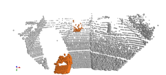
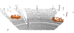
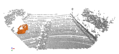
$M^{Q}_{fg}$
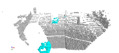
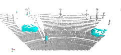
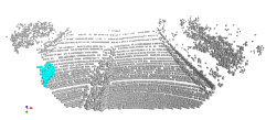
Error Map

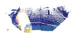
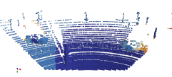
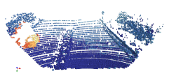
Figure I: Three examples from $\mathrm{lidarKITTI}$ [Geiger et al.(2012)Geiger, Lenz, and Urtasun] show the cases where cars are not fully sensed in the second frame $Q$ and our scene flow prediction partially fails. For visual enhancement only, we show the RGB images of each scene. We visualize the predicted binary mask, where $BG$ and $FG$ points are encoded by gray and orange or cyan colors, respectively. The error map for each scene (third row) shows the end-point error in meters and is colored according to the map shown in the last row.

Adding robustness against occlusions remains a challenge for future work.

II.4 Additional Qualitative Results

We visualize our predicted masks and the error maps of scene flow of six examples from $\mathrm{stereoKITTI}$ in Figure II and another six examples from $\mathrm{lidarKITTI}$ in Figure III.

	Example 1	Example 2	Example 3
Scene
$M^{P}_{fg}$
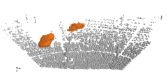
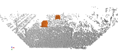
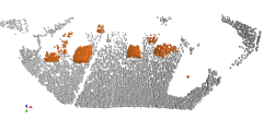
$M^{Q}_{fg}$
Error Map
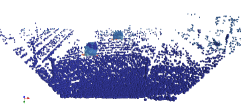
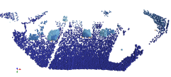
	Example 4	Example 5	Example 6
Scene
$M^{P}_{fg}$
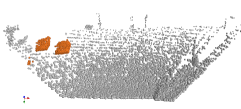
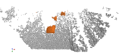
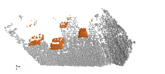
$M^{Q}_{fg}$
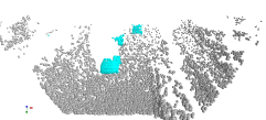
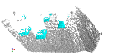
Error Map

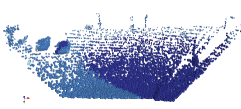
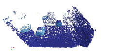
Figure II: Six examples from $\mathrm{stereoKITTI}$ [Menze and Geiger(2015)] show the qualitative results of our EgoFlowNet.

	Example 1	Example 2	Example 3
Scene			ng
$M^{P}_{fg}$
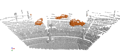
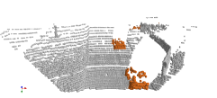
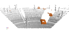
$M^{Q}_{fg}$
Error Map
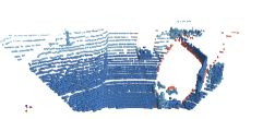
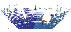
	Example 4	Example 5	Example 6
Scene
$M^{P}_{fg}$
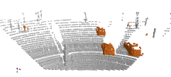
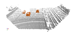
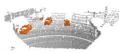
$M^{Q}_{fg}$
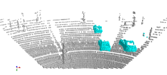
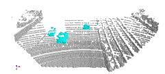
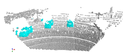
Error Map

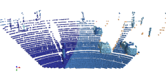
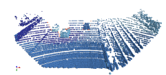
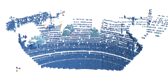
Figure III: Six examples from $\mathrm{lidarKITTI}$ [Geiger et al.(2012)Geiger, Lenz, and Urtasun] show the qualitative results of our EgoFlowNet.

References

- [Battrawy et al.(2022)Battrawy, Schuster, Mahani, and Stricker] Ramy Battrawy, René Schuster, Mohammad-Ali Nikouei Mahani, and Didier Stricker. RMS-FlowNet: Efficient and Robust Multi-Scale Scene Flow Estimation for Large-Scale Point Clouds. In IEEE International Conference on Robotics and Automation (ICRA), 2022.
- [Behl et al.(2019)Behl, Paschalidou, Donné, and Geiger] Aseem Behl, Despoina Paschalidou, Simon Donné, and Andreas Geiger. PointFlowNet: Learning Representations for Rigid Motion Estimation from Point Clouds. In IEEE/CVF Conference on Computer Vision and Pattern Recognition (CVPR), 2019.