Data-driven Software-based Power Estimation for Embedded Devices

Abstract

Energy measurement of computer devices, which are widely used in the Internet of Things (IoT), is an important yet challenging task. Most of these IoT devices lack ready-to-use hardware or software for power measurement. A cost-effective solution is to use low-end consumer-grade power meters. However, these low-end power meters cannot provide accurate instantaneous power measurements. In this paper, we propose an easy-to-use approach to derive an instantaneous software-based energy estimation model with only low-end power meters based on data-driven analysis through machine learning. Our solution is demonstrated with a Jetson Nano board and Ruideng UM25C USB power meter. Various machine learning methods combined with our smart data collection method and physical measurement are explored. Benchmarks were used to evaluate the derived software-power model for the Jetson Nano board and Raspberry Pi. The results show that 92% accuracy can be achieved compared to the long-duration measurement. A kernel module that can collect running traces of utilization and frequencies needed is developed, together with the power model derived, for power prediction for programs running in real environment.

I Introduction

Measuring the energy consumption of computer systems has always been an important task, as:

• Energy consumption is an important indicator of system performance [1] [2] [3]. In the realms of head-mounted AR [4] and edge computing [5], energy efficiency directly influences the operational capabilities and sustainability.

• Some energy-aware system design methodology makes control based on energy consumption feedback [6] [7] [8].

High-end and accurate hardware-based measurement [9] [10] [11] is one solution, but such hardware is often expensive and requires specialized operation and integration knowledge. To allow users to measure the energy consumption of their devices without the need of specialized hardware, vendors offer several software-level solutions, such as Intel RAPL [12] and AMD uProf [13]. Such tools estimate energy consumption through statistics collected from runtime hardware devices. Building a software-level energy analysis tool is often accompanied by building an energy model [14] [15] [16] [17] and ensuring that the hardware devices can provide the parameters needed for that model with low overhead.

Unfortunately, as of today, many popular embedded hardware (for example, Raspberry Pi and Nvidia Jetson Board) [12] [18] [19] that is widely used in IoT and Mobile Edge Computing (MEC) System, lacks a software-level approach for energy measurement. In this case, users who do not have access to high-end equipment can only measure power consumption based on consumer-grade meters [20] [21] [22]. We next discuss the limitations of using consumer-grade meters.

I-A Limitations of using consumer-grade power meters for energy measurement

Consumer-grade power meters often do not provide data API. To integrate power measurement into energy-saving policy design, a practical solution will be using the data interface provided by the meter (similar to the sysfs interface in Linux) for programs to access power meter measurement. Unfortunately, we did not find a consumer-grade energy meter that offers a data API. In most cases, the power meter provides a GUI interface for the user to read data from the hardware or software connected to the meter via Bluetooth [23]. The lack of a low-overhead and low-latency data access scheme means that making a policy design approach feasible based on energy feedback for control is challenging with consumer-grade power meters.

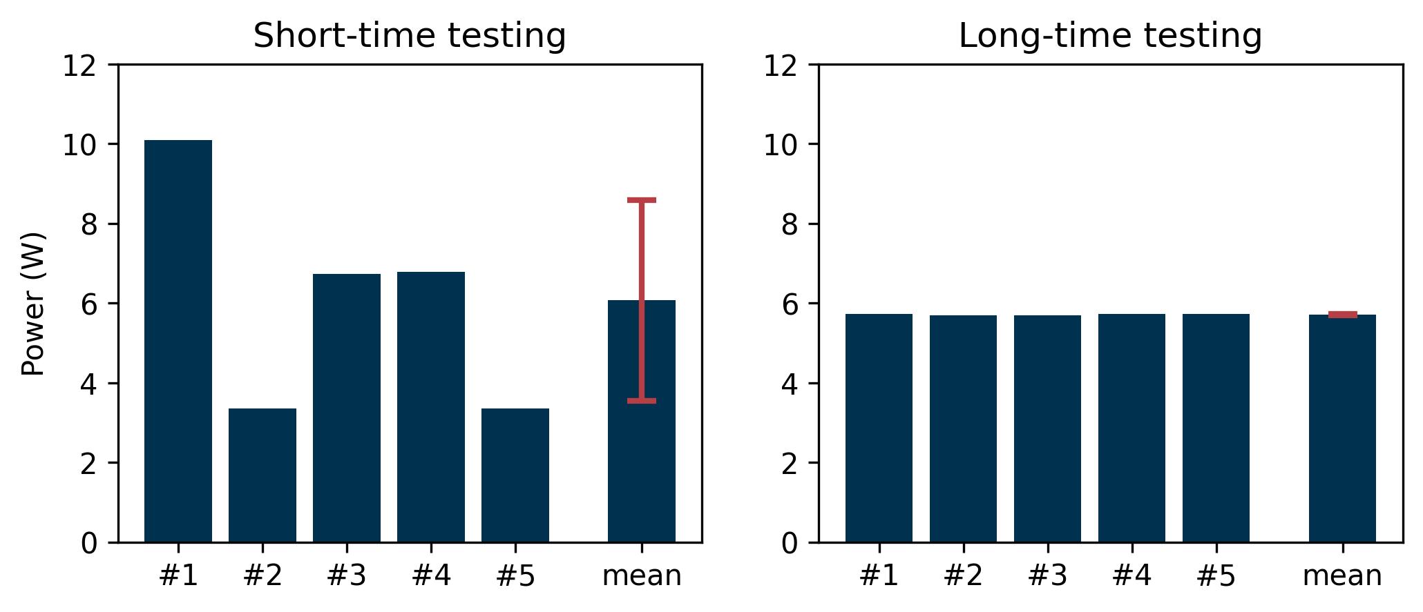
Figure 1: Power measuring using a consumer-grade meter.

Consumer-grade power meters cannot provide accurate short-duration measurement.

Due to hardware limitations, consumer-grade meters record voltage/current changes in a coarse-grained view, usually in seconds. This means it is difficult to accurately measure energy consumption over short periods of time. Next we illustrate this point using an example of measuring the energy consumption of a CPU-intensive program with an execution time of around 1 second. We applied two methods. One is based on short-duration measurement, where we simply record the energy consumption during the 1-second execution. Another one is based on long-duration measurement, where we run the workload repetitively in a loop for three minutes and obtain the average energy consumption for 1-second execution as the total 2-minute energy consumption divided by the number of executions. The test is shown in Fig. 1. The variance of measurements over short periods of time is much larger than over long periods of time. This illustrates that short-duration measurement is not reliable and only measurements over a long period of time can provide an accurate, consistent result.

Because of the above-discussed limitations, energy measurements in our previous works [24] [25], were very labor intensive.

I-B Proposed approach

In this paper, we propose a data-driven method to derive software-based power estimate model using only consumer-grade meter. The contributions of the paper can be summarized as follows.

• For users or researchers with devices that do not have software-based energy measurement support and have access only to consumer-grade meters, our method can help them construct a software-based energy consumption estimation model for their devices.

• Our estimation model allows short-duration estimation, overcoming the limitation of the consumer-grade power meters.

• Our method is based on smart data collection and data analytics techniques to estimate power. Our data collection method is simple yet able to sample the parameter space evenly.

• Our energy estimation model can be used to obtain timely feedback on energy consumption, which is especially useful for AI researchers to design or improve energy control policies as it avoids the inconvenience of integrating hardware-based measurements.

I-C Related works

Unlike design solutions that are based on mathematical models for offline analysis[26] [27] [28] [29] [30] [31] [32] [33] [34], adaptive system design and measurement methods based on machine learning [24] [25] [35] [36] [37] [38] [39] [40] [41] [42] [43] [44] have received attention in recent years. Accurate power modeling and measurement have been widely explored in the literature, with various approaches proposed for different types of processors and systems. Below, we review some key contributions and compare them with our proposed method.

Rethinagiri et al. [45] built power models for ARM-based processors, such as Cortex-A8 and Cortex-A9. They measure static and dynamic currents with an Agilent LXI digitizer and use a multimeter to measure the voltage on the jumpers to get the power. The parameters used to build the model are frequency, instructions per cycle (IPC), cache miss rate, etc. The models are built differently for different processors. They built accurate models for the processors and used measuring instruments with high precision. In contrast, our work proposes a method that allows researchers who can only use consumer-level devices to construct energy consumption models for their own devices. Also, the parameters we chose are common to all processors, while their work chose parameters based on the specific processor, including some low-level parameters.

Walker et al. [46] also derived models for ARM-based processors. Their approach is noteworthy because they collected data from multiple PMCs and then constructed algorithms to select the PMC parameters that were ultimately put into the model. Nikov et al. [47] constructed a linear regression model for Cortex-M0 using a total of 6 parameters such as executed instructions, multiplication instructions, taken branches and RAM data reads. They measure energy consumption using a custom measurement board.

There are some methods to build a power model from the RTL level. Zoni et al. [48] proposed a method that could implement a power model based on the RTL description of the target architecture. Kim et al. [49] collected 50 signals at the RTL level and then proposed a method to select the signals to build the model automatically. These methods are characterized by a more complex model-building process and require domain-specific knowledge. In contrast, our proposed approach is easy to follow, reproducible, and does not require much domain-specific knowledge of CPU architecture.

Some works also build power models, but they do not use real machine measurements. They use simulated power [50] [51] [52] or simulators [53]. Simulated models provide insights and theoretical frameworks but often lack the accuracy and real-world applicability of models built with actual hardware measurements. Our approach is performed on real devices for energy measurement as well as model testing, ensuring practical applicability and accuracy.

In summary, while existing methods provide high accuracy and detailed models, they often involve high costs, complexity, and specialized knowledge. Our approach offers a practical alternative that balances ease of use, cost-effectiveness, and accuracy, making it suitable for embedded and IoT devices lacking built-in power measurement capabilities.

II Data-driven Power Estimation with Consumer-grade Meters

Our data-driven method to derive a software-based power estimate model using only consumer-grade meters is divided into three main steps.

1. Collect data related to workload execution and energy using long-duration energy measurement with power-meter.

2. Construct energy model based on collected data from the devices and the power meter.

3. Estimate the power of the workloads using the model constructed and a software module that can track workload executions.

The hardware connection for the approach is shown in Figure 2. The power meter is connected to the underlying device to be studied. Note that workload will run on the device for data collection to construct energy model for the device. A PC is used to receive the Bluetooth data sent by the power meter, which is energy consumption data. In addition, the parameters (frequency and utilization of the device) that are used to build the model, are recorded when the workload runs on the device. These data are integrated together with the energy consumption data for energy model construction. A data collection module is required to retrieve the necessary parameters like the frequency and utilization data for using the model.

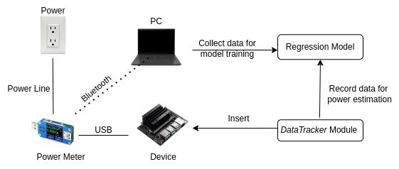
Figure 2: An illustration of the methodology

II-A Training Data Collection

The way to collect training data is to run benchmark programs and measure the energy consumption with a power meter while collecting corresponding parameter traces while the benchmark runs. There are many factors that can affect power, such as voltage, current, frequency, utilization, etc. Among these parameters, we choose frequency and utilization because there is a strong correlation between these two parameters and the power. Utilization is an empirical choice and there are other studies [54] that consider utilization when constructing power models or energy models. Based on the equations of the CMOS circuit model [55], frequency and power show a sub-square relationship, which means frequency and power are strongly correlated.

In order to collect observations of evenly distributed utilization and frequency levels, we choose CPU-intensive workloads as our benchmarks so that we can control the frequency and utilization easily. One of the benchmarks is a single-threaded benchmark, which performs multiple multiplications. This benchmark’s utilization on a single core is 100%. The embedded device that we perform our experiments is a Nvidia Jetson Nano Board 2GB. The number of cores on the board is 4. Thus, the average utilization for the four cores is 25%, which means the highest utilization for running this benchmark is 25%. The other benchmark is a multi-threaded benchmark, which runs multiple multiplication programs, each of which is 100% CPU-intensive on one core. In our experiments, there are 4 threads in total.

Since the data to be collected are related to frequency and utilization, we controlled (regulated) both frequency and utilization levels (evenly distributed) to different values for data collection, which is shown in Algorithm 1. In this algorithm, the frequency is controlled by setting the DVFS governor to $userspace$ and then running the benchmark at each frequency. Controlling utilization levels is relatively more complicated. Different utilization levels are obtained by setting a proper combination of runtime and idle time. For example, an approximate utilization of 50% can be obtained by first running the benchmark and then letting the device stay idle for the same amount of time. The purpose of regulating the frequencies to all available levels and utilization to evenly spaced values is to allow simple data sampling with good data distribution.

The total runtime of each workload is set to 180 seconds. The runtime is controlled by a $factor$, ranging from 0 to 10. By multiplying a different $factor$, the runtime of the benchmark will be different. The idle time is obtained by subtracting the run time from the total time.

In the algorithm, $read\_energy()$ is done through power meter measurements. The utilization is retrieved from the $/proc$ file system.

Algorithm 1 Power Measurement for Regulated Frequency and Utilization Levels

1:set $total\_time$ to 180 seconds

2:set $runtime\_factor$ to 18

3:set governer to userspace

4:for each $frequency$ that the device support do

5:     set $frequency$

6:     for $factor$ from 0 to 10 do

7:         $energy\_start$ $\leftarrow$ read_energy()

8:         $time\_start$ $\leftarrow$ time.time()

9:         while $time.time()-time\_start<factor\times runtime\_factor$ do

10:              run the benchmark

11:         end while

12:         $time.sleep(total\_time-$

13:$\qquad\qquad\qquad factor\times runtime\_factor)$

14:         $energy\_end$ $\leftarrow$ read_energy()

15:         $time\_end$ $\leftarrow$ time.time()

16:         $power\leftarrow\frac{energy\_end-energy\_start}{time\_end-time\_start}$

17:         $utilization$ $\leftarrow$ system recorder

18:         record ($power$, $frequency$, $utilization$)

19:     end for

20:end for

II-B Derive Power Model from Collected Data

After obtaining the training data, various methods can be explored to derive a model to predict the power for a given utilization and frequency. The models that we explored include regression models, decision tree models, and neural network models. Note that the types of models to be used are not limited to the above. The details of deriving models for a Jeston Nano board will be described in section III. Here we show the regression model as an example.

$$Power= k_{0}\cdot utilization^{2}+k_{1}\cdot frequency\cdot utilization$$ (1)

$$+k_{2}\cdot utilization+b$$

Different regression models were explored for the Jeston nano board. Among them, the best results were obtained from the per-frequency regression model. In this model, at each frequency the device supports, there is a polynomial expression consisting of utilization, as shown in Equation 1.

At each frequency, there are corresponding values for $k_{0}$, $k_{1}$, $k_{2}$ and $b$. The reason for choosing such a regression model is that the change in frequency causes a jump of the power, which will be explained in detail in Section III-C1.

II-C How to Use the Software-based Power Model?

Our model is constructed based on benchmark programs measured at a single frequency. However, in a real environment, programs do not often run at a fixed frequency because Operating Systems may dynamically change the frequencies based on system demand. Our model can also predict power for such running scenarios, but the operation becomes relatively complex.

To predict the power for programs running with multiple frequencies, it is necessary to obtain multiple frequencies for the running trace, the utilization for each frequency and the duration of the frequency. With the utilization of each frequency segment, the power over this frequency period can be obtained based on our model.

The total power of the program can then be calculated by Equation 2, where $n$ represents the total number of frequency segments, $P_{i}$ represents the predicted power of the segment which is calculated based on the constructed model, and $t_{i}$ represents the duration of the segment.

$$Power=\frac{\sum_{i=1}^{n}p_{i}\times t_{i}}{\sum_{i=1}^{n}t_{i}}$$ (2)

To get the duration and utilization information for a running traces, we built a kernel module called DataTracker module that can directly track all the frequencies used together with their duration and the utilization of each core at each frequency change. The detailed information of this module will be explained in Section IV-A.

III Building Power Model

In this section, we illustrate our method by showing how to construct power models based on regulated data collection. We use a Jetson Nano Board (2GB) as an example.

III-A Training Data Collection

The data collection includes setting frequency and utilization for a given workload and measuring the energy consumption of running the workload. We choose frequency and utilization as parameters as they are the two most important parameters that affect CPU energy consumption during a period of time when running a workload under a DVFS policy. Note that CPU energy consumption consumes the vast majority of energy among all the components of the device, especially when there is no display. Therefore, the model we build will be a good approximation of the energy model device, even though we do not take the detailed model of the CMOS circuit and board architecture as input.

III-A1 Time for Running Workload

The total run time for each workload is set to 3 minutes. The duration for measurement is set to such a consistently long time because the power meter cannot accurately measure the energy consumption of workloads that run for a short period. The longer the test time, the more accurate it will be. Such a setting guarantees that each measurement of collected energy consumption is sufficiently accurate.

III-A2 Frequency Control

Controlling the frequencies can be achieved by setting the frequency of the workload with the User Governor provided by Linux. The workload will be running with each available frequencies.

III-A3 Utilization Control

To collect data that covers the parameter space evenly, as discussed in Section II-A, we divide the utilization into several levels with equal distance in between and measure the energy consumption for each combination of utilization and frequency. This method avoids the need to use multiple benchmarks to collect data with different utilization and is more convenient. But note that the level to which we want to control the CPU utilization can only be approximate. For example, if we want to get a 10% utilization by controlling the running pattern of workload, the real CPU utilization could be 8%. Thus, we use the target utilization to control the workload and measure the resulting exact utilization for each controlled workload. The utilization data collected for training is the exact utilization for the controlled workload. How to control the utilization of a workload was described by Algorithm 1 in Section II-A.

III-A4 Training Data Illustration

The embedded device, Nvidia Jetson Nano Board 2GB (JTN), supports a range of frequencies from 0.102 GHz to 1.479 GHz. The number of CPU cores is 4. Training data collection is done based on the algorithm explained in Section II-A. The training data are shown in Fig. 3. This is a 3D figure with the x, y, and z axes representing frequency, utilization, and power, respectively.

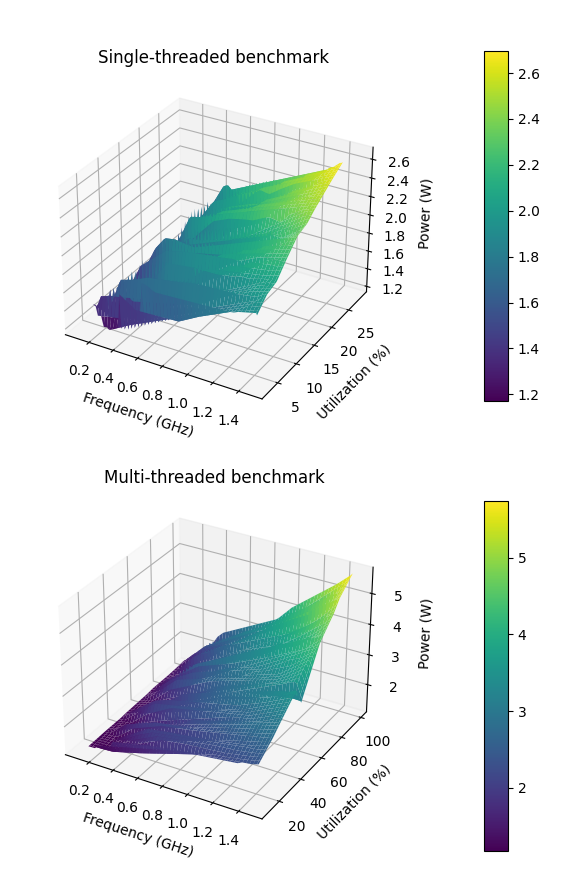
Figure 3: Measurement results of single-threaded (top) and multi-threaded (bottom) benchmark

It can be seen that as the frequency and utilization increase, so does the power. When the frequency is constant, the utilization and power are smoothly related. When the utilization is roughly within a range, there is a jump in power as the frequency changes. This is obvious in the single-threaded benchmark. The first three frequencies correspond to a power level, and the latter frequency corresponds to another power level. We inferred that the reason for this jump is the change in voltage. Comparing the single-threaded data with the multi-threaded data, we can see that the multi-threaded data has a steeper trend.

We only used multi-threaded data and not single-threaded data when constructing the model as they span across a wide range of utilization.

III-B Testing Data Collection

We chose to select benchmarks from Mibench [56] and Sysbench [57] as the testing data. These two test sets were chosen because they are both commonly used, lightweight and easy to measure. Mibench contains different types of benchmarks, most of them are single-threaded, while the benchmarks in Sysbench are multi-threaded.

We selected 10 benchmarks from Mibench, which are $basicmath$, $bitcount$, $jpeg$, $typeset$, $dijkstra$, $particia$, $stringsearch$, $blowfish$, $sha$ and $crc32$. These 10 benchmarks cover all types in Mibench.

The benchmarks selected from Sysbench are $cpu$, $memory$ and $fileio$, where $cpu$ performs a series of CPU-intensive computational tasks, $memory$ performs a series of memory-related operations and $fileio$ performs file read and write operations. Since Sysbench is a multi-threaded benchmark test, the number of threads can be set to different values. In the experiment, we set it to 1, 2, 3, and 4 to get multi-threaded data.

We set the CPU frequency to each available level when running each Mibench (or Sysbench) benchmark. We then obtain the utilization and power for each running case. The utilization is obtained by reading from the $/proc$ file system, and the power is obtained by a long-time measurement with the power meter. At each frequency, each benchmark is run multiple times for 3 minutes. The purpose of this is to reduce errors introduced by single or short-time measurement. The method of reading energy consumption is the same as in Section II-A. Fig. 4 shows the measurement results of the Mibench benchmarks.

The testing data collected will be used to evaluate the software estimation models developed in the next subsection.

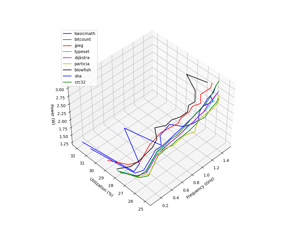
Figure 4: Measurement results of 9 benchmarks in Mibench

In general, the measurements of the utilization of these 9 benchmarks are more stable and do not vary much.

The one remaining benchmark in Mibench, $stringsearch$, has a different trend from these nine benchmarks, as shown in Fig. 5. The other benchmark is $bitcount$ of the other 9, selected to be used as a comparison. It can be seen from the figure that the power of $bitcount$ is shown as the previous illustration where it has a jump. However, the power of $stringsearch$ show a different trend. Its power consumption increases progressively with increasing frequency. The reason is that the other benchmarks show little change in utilization at all frequencies. However, $stringsearch$ has higher utilization at lower frequencies than the other benchmarks. At high frequencies, its utilization is reduced. Therefore no jump in energy consumption of this benchmark.

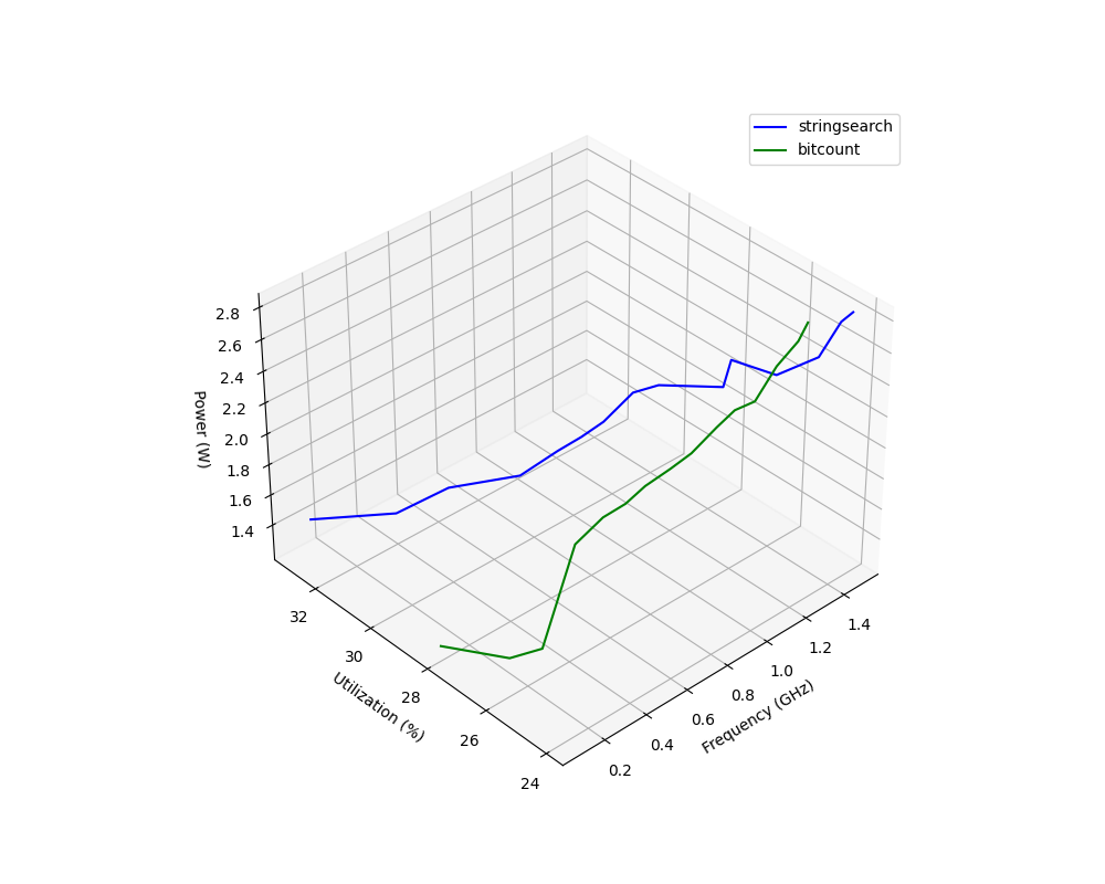
Figure 5: $stringsearch$ vs $bitcount$

The measurement results of Sysbench are shown in Fig. 6. It can be seen from the figure that for $cpu$ and $memory$, their thread count is reflected in the variation of utilization, which is 30% utilization for a single thread, 60% utilization for 2 threads, 80% utilization for 3 threads and 100% utilization for 4 threads. Their power also appears as a jump with frequency.

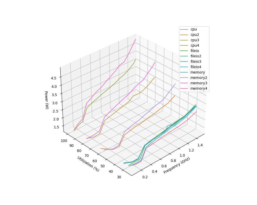
Figure 6: Measurement results of Sysbench

III-C Model Derivation and Evaluation

We use the data collected (illustrated in Section III-A4) to build the models and the test data from Section III-B to evaluate the accuracy of the models. The metrics used are mean squared error (MSE), mean absolute error (MAE), and $R^{2}$ score [58].

Mean Squared Error (MSE) is the average of the squares of the errors—that is, the average squared difference between the estimated values and the actual value. Mean Absolute Error (MAE) is the average of the absolute errors—the average absolute difference between the estimated values and the actual value. The $R^{2}$ score indicates the degree of explanation of the dependent variable by the independent variable. It ranges from 0 to 1. The higher the value of this indicator, the higher the degree of prediction accuracy.

III-C1 Polynomial Regression Model

We constructed four linear models based on the training data. The first model we choose is the simplest polynomial model. We call Model 1 the Simple Regression Model. Frequency and utilization as two parameters are selected in the model as cubic and primary, respectively. This is because, in the CMOS circuit model, frequency and power consumption are cubic. The second model is optimized based on Model 1. It added more terms with different exponents, with the highest order being 3. The reason for this modification is simply the intuitive idea that adding more terms will improve the accuracy of the model. We call Model 2 the Multi-Term Regression Model. Considering the frequency/voltage levels, we further divide Model 2 into two different equations corresponding to 2 frequency/voltage levels. It uses one set of coefficients when the frequency is in the first 3 levels, and another set of coefficients when the frequency is in the later levels. We call it the Multi-Frequency Regression Model. We improve Model 3 further and introduce Model 4, called the Per-Frequency Regression Model, which fits data to individual frequency.

All results of four models based on testing data can be seen from Table I.

TABLE I: The accuracy of regression models

Model	MSE	MAE	$R^{2}$ score
Simple Regression Model	0.2397	0.4184	-0.0242
Multi-Term Regression Model	0.0272	0.1365	0.8839
Multi-Frequency Regression Model	0.0270	0.1344	0.8848
Per-Frequency Regression Model	0.0182	0.1040	0.9221

The results show that Per-Frequency Regression Model performs much better than the previous three models, with the lowest MSE and MAE and the highest $R^{2}$ score.

III-C2 Decision Tree Model

The following two models use the decision tree model. The accuracy of 2 decision tree models is shown in Table II.

TABLE II: The accuracy of decision tree models

Model	MSE	MAE	$R^{2}$ score
Decision Tree Model 1	0.1361	0.3052	0.4187
Decision Tree Model 2	0.0433	0.1668	0.8149

Decision tree model 1 is a model fitted by a machine learning algorithm based on XGBoost [59]. It trains and integrates decision tree models using gradient-boosting methods and generates a forest for making a decision.

The results show that this model performs worse than the regression models 2-4, with an MSE of 0.1361 and MAE of 0.3052. Its $R^{2}$ score of 41.87%, which is low. Obviously, this model does not work well.

Decision tree model 2 enhances Decision tree model 1 by applying the XGBoost algorithm for each frequency, using a similar idea in the construction of polynomial regression model 4. The results show that Decision Tree Model 2’s performance is much better than Decision Tree Model 1, with a lower mean squared error of 0.0433 and a slightly lower mean absolute error of 0.1668. Its $R^{2}$ score of 0.894.

III-C3 Neural Network Model

The above six models constructed are based on explicit parameters: frequency and average utilization. We also tried to construct models with more input data. We replace the original average utilization with the utilization per core. Because of the more input parameters used, we train it with a neural network model.

We use the same training data as before, that is measurements from the multi-threaded CPU-intensive benchmark. The utilization of each core has been recorded in the previous measurements. The defined neural network has 5 inputs and 1 output. The 5 inputs correspond to the frequency and the utilization of the 4 cores and the 1 output is the predicted power consumption. The middle layer consists of a total of 4 hidden layers with 128, 64, 32 and 16 neurons.

The Neural Network model is trained 4000 times with the training data. The model was then tested with the testing data. The MSE is 0.0328, MAE is 0.1346. This model is not as effective as the best regression model 4, but it is still a plausible model.

IV Power Prediction for Programs running in Real-World Environment

An operating system that supports power governors can regulate frequency to save energy. Thus, a program is unlikely to run with only one frequency. Predicting the power of programs running with variable frequencies is important. This section introduces our method for predicting the power of programs running in a real environment using the device’s derived power model together with a data tracker software module.

IV-A Kernel-Level Data-Tracker Module

We have developed a Kernel-level Data Tracker module to monitor real-time CPU frequency changes and log the corresponding CPU load data. The Kernel-level Data Tracker, together with the derived power model, is essential for software-based energy prediction. This module leverages the Linux $cpufreq$ API, specifically utilizing the $get\_cpu\_idle\_time$ function, which retrieves the CPU’s idle time over a period. By tracking these changes, the module provides data for power estimation and performance analysis.

Each CPU in the system has a dedicated $cpu\_data$ structure that stores the previous idle and total times of the CPU. This structure is crucial for calculating the CPU load, as it allows the module to determine the difference in idle and total times between frequency changes.

IV-A1 Core Mechanism

When the CPU frequency changes, a callback function $frequency\_notifier$ is triggered, which responsible for recording the old frequency, the duration for which it was maintained, and the CPU load during this period. The following steps outline the process:

• Frequency Change Detection: The module registers a notifier for CPU frequency transitions using the $cpufreq\_register\_notifier$ function. This notifier is called whenever the CPU frequency changes.

• Data Logging: The notifier function logs the old frequency, the duration it was active, and the load of each CPU. The data is formatted into a string and written to a specified file path data_file_path using Linux file system APIs.

• CPU Load Calculation: The CPU load is calculated by comparing the current idle and total times with the previously recorded values. This calculation is performed using the $cpu\_load$ function, which ensures that negative values are handled appropriately and that the load percentage does not exceed 100%.

IV-A2 Data Persistence

To persist the tracked data, the module writes the information to a file specified by data_file_path. The file operations are performed in kernel space using the $vfs\_write$ function. The data is appended to the file, ensuring that all frequency changes and corresponding loads are recorded sequentially.

IV-A3 Proc File System Interface

The module provides an interface through the $proc$ file system, allowing users to control the logging functionality. By writing specific symbols (’1’ to start logging, ’0’ to stop logging) to the $cpufreq\_monitor$ proc file, users can enable or disable the logging process dynamically. This interface is implemented in the $procfile\_write$ function, which interprets user input and updates the logging state accordingly.

IV-A4 Stability and Error Handling

To enhance the stability and reliability of the module, several error handling mechanisms are included:

• Negative Time Handling: The $cpu\_load$ function checks for negative values in idle and total time calculations. If such values are detected, a warning is logged, and appropriate measures are taken to ensure the calculations remain valid.

• Load Percentage Bounds: The module ensures that the calculated CPU load does not exceed 100%. If an anomaly is detected, such as a load percentage greater than 100%, a warning is logged for further investigation.

• File Operation Errors: The $log\_data$ function includes checks to handle errors that may occur during file operations, such as failure to open the file. Appropriate error messages are logged to help diagnose issues.

IV-A5 Portability

The module is built using standard Linux kernel APIs, making it highly portable across different hardware platforms. It can be deployed on x86, ARM, or any other Linux-enabled architecture without requiring hardware-specific modifications. This portability ensures that the module can be used in a wide range of environments, from desktop systems to embedded devices.

This module offers a robust solution for monitoring CPU performance, enhancing the understanding of power consumption and enabling optimized resource management across diverse computing environments. The Data Tracker module’s design and implementation reflect a significant contribution to performance analysis tools, providing a reliable and versatile mechanism for real-time CPU monitoring.

IV-B Example: Power Prediction for programs with Multiple Frequencies

Figure 7 shows a portion of the real trace derived from the Data Tracker module. The trace includes the utilization and frequency of a workload (top) and the predicted power values (bottom) for each frequency segment. The trace is the experimental result for the benchmark $basicmath$ running with variable frequencies under the $ondemand$ governor. The x-axis represents time, while the y-axis conveys information about each frequency segment. In the upper part of Figure 7, the height of the orange bar indicates the frequency level, and the height of the blue bar denotes the utilization at that frequency. The lower part of Figure 7 shows the predicted power values (depicted by the red dashed line) for each frequency segment, calculated using our constructed power model.

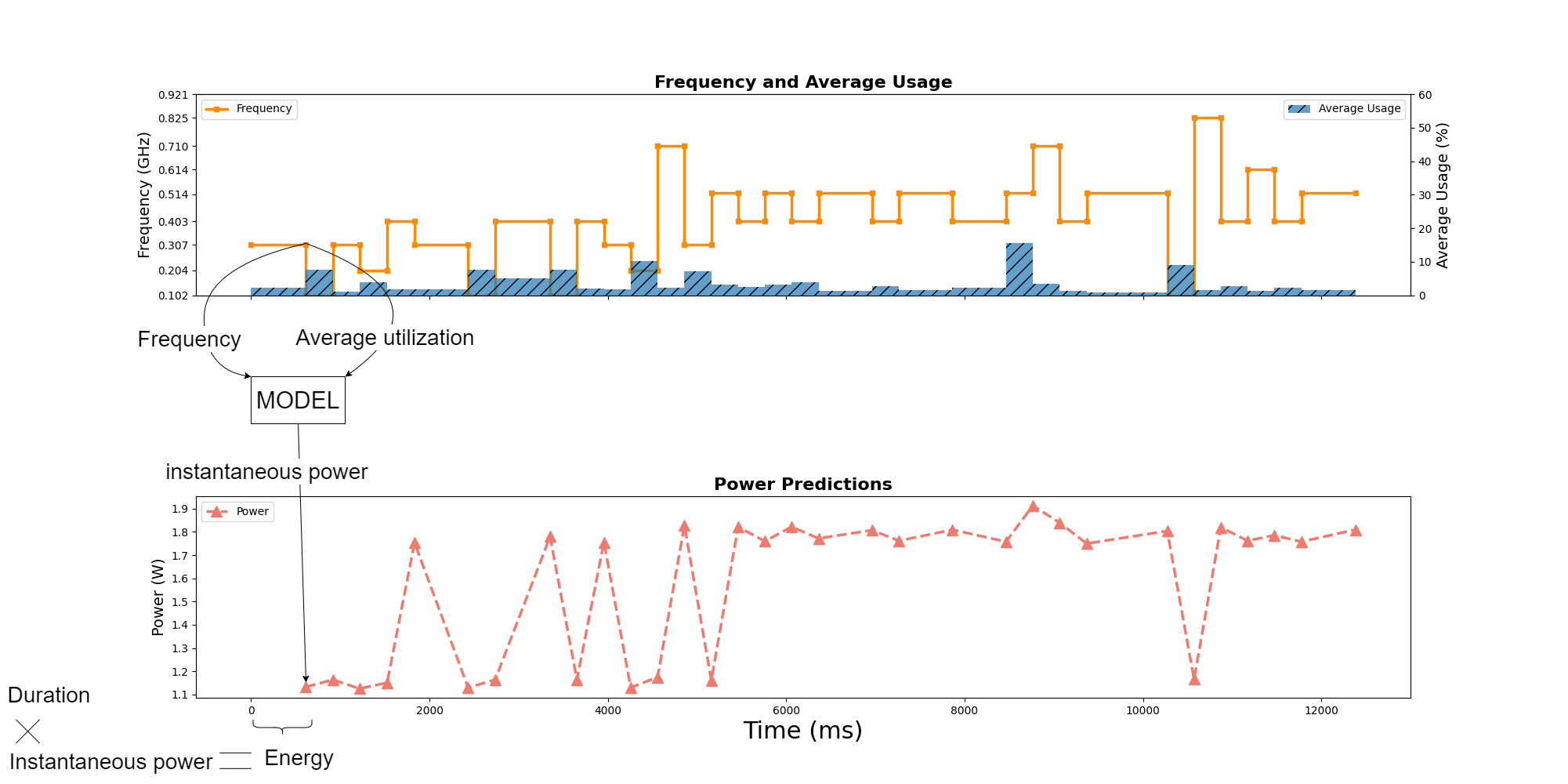
Figure 7: A real trace of utilization and frequency and it’s prediction

The predicted power value based on the entire trace of collected data is 2.137. The measured true value is 2.285. The power prediction model used is the Per-frequency Regression Model (Model 4). The low prediction error demonstrates that our model is applicable for power prediction under multiple frequencies with high accuracy.

V Evaluation of Power Prediction and Discussion

In this section, we rigorously evaluate our models by comparing the predicted results with empirical data for programs executed under variable frequencies and discuss the implications of our findings. The evaluation includes testing programs that runs under the Linux $ondemand$ governor, which dynamically adjusts frequencies based on system utilization. We also deploy our approach on a different embedded platform to validate its reproducibility.

V-A Evaluation Under $ondemand$ Governor

We tested various benchmarks running under the Linux $ondemand$ governor to assess the accuracy of our power prediction model. The $ondemand$ governor dynamically adjusts the CPU frequency based on system utilization, which necessitates capturing all frequencies, utilizations, and durations for which the underlying program is executed. We achieved this by incorporating the data tracking module previously discussed in Section IV-A, which records data each time a frequency change occurs.

Figure 8 shows the comparison between the measured data and the predicted data for 11 benchmarks. The red bars represent the measured data, while the blue bars indicate the data predicted by our model. As observed, the predicted and actual values are closely aligned, signifying the high prediction accuracy of our model.

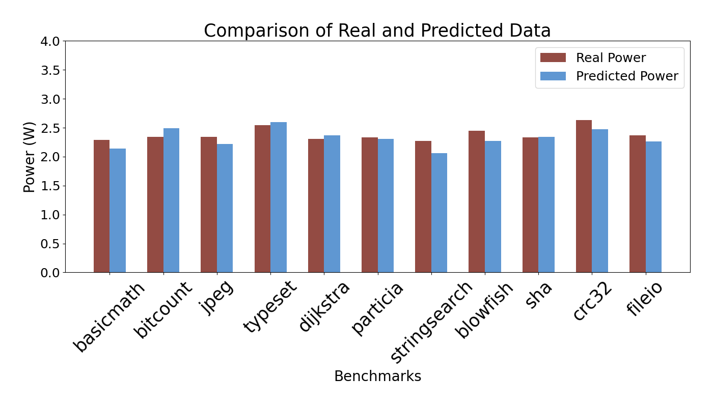
Figure 8: Benchmark predictions vs real values on JTN

Table III presents the absolute error for each benchmark’s prediction. The mean absolute error across all benchmarks is 0.1118, and the mean squared error is 0.0164. These metrics confirm that the prediction error is minimal, thereby validating the high prediction accuracy of our model.

TABLE III: Absolute error

Benchmark	AE	Benchmark	AE
$basicmath$	0.148	$bitcount$	0.1506
$jpeg$	0.1236	$typeset$	0.0499
$dijkstra$	0.0576	$patricia$	0.0341
$stringsearch$	0.2163	$blowfish$	0.1739
$sha$	0.0091	$crc32$	0.1592
$fileio$	0.1063

V-B Reproducibility on Different Platforms

To further validate our approach, we also deployed it on a different embedded platform, specifically, the Raspberry Pi. The validation process includes data collection, model building, prediction of simulated behavioural data, and prediction of real behavioural data.

Figure 9 presents the benchmark predictions versus real values on the Raspberry Pi. The results indicate that the average mean error is approximately 4%, with the best test achieving an average error of 2%. These results demonstrate that the methodology is applicable to different embedded platforms for achieving accurate energy consumption predictions.

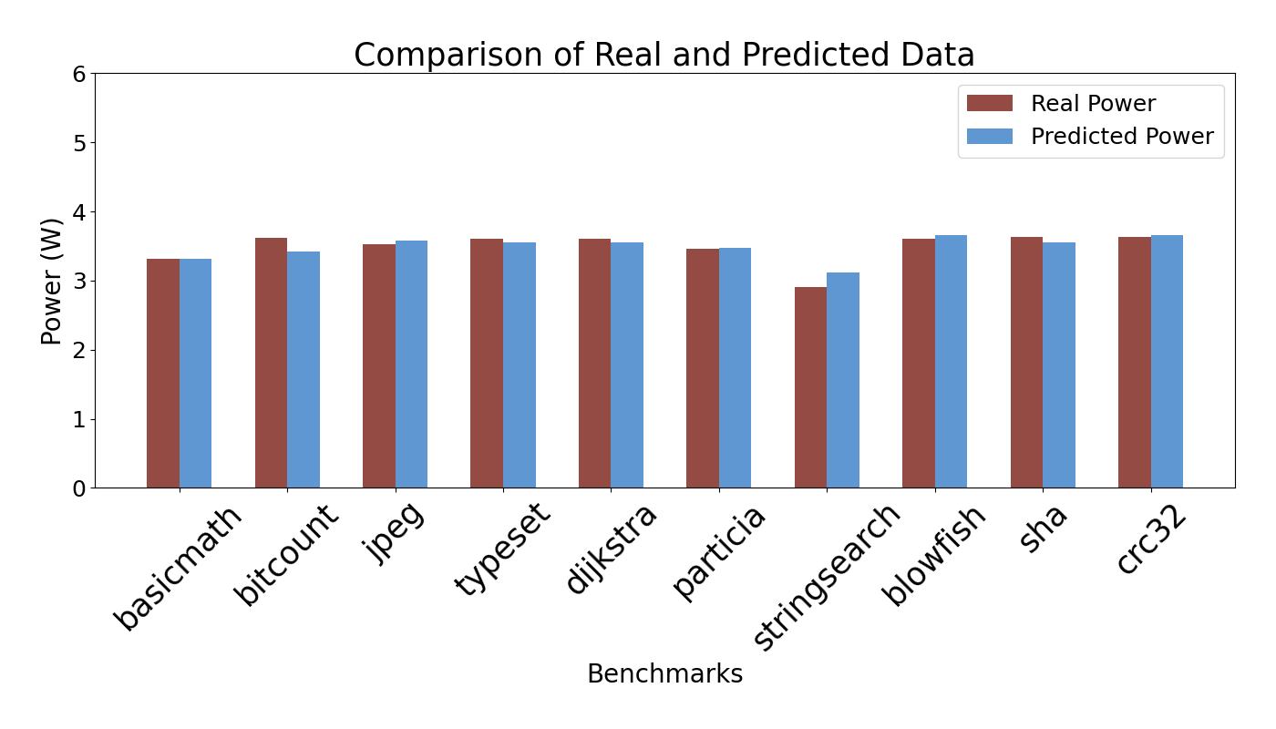
Figure 9: Benchmark predictions vs real values on RBP

However, certain discrepancies were observed. For instance, the $fileio$ benchmark behaves differently on the Raspberry Pi. This is due to the specific behavior of file I/O operations on this platform.

Overall, our model demonstrates high prediction accuracy under varying conditions and on different platforms, validating its robustness and applicability.

VI conclusion

Most small inexpensive embedded devices in MEC systems do not have software-based power measurement support. This paper proposes a smart data-driven method using consumer-grade meters to construct software-level power estimation models for such embedded devices. We first describe the two drawbacks associated with the use of a power meter to measure energy consumption, which are the inability to measure instantaneous power consumption and the inability to act on energy feedback-based systems. Then, we describe our approach to constructing the power model by systematically generating workloads and collecting training data. To use our approach, one can follow the steps described in this paper to build the model for their own devices. The steps include building the workload, collecting training data, constructing the model and using the model. During the experiments, we explored several types of models, and in the end, the model that worked best on the device that we tested was a per-frequency polynomial regression model on utilization. The model accuracy is 92% compared to the long-duration measurement. The approach is simple and systematic, capable of achieving good results in predicting energy consumption, thus allowing the researchers/application developers to avoid using a power meter for power management. We also provide a platform-independent kernel module that can be used to collect running traces of utilization and frequencies needed for power prediction for programs running in Linux environment.

References

- [1] M. Weiser, B. Welch, A. Demers, and S. Shenker, “Scheduling for reduced cpu energy,” Mobile Computing, pp. 449–471, 1996.
- [2] V. M. Weaver, M. Johnson, K. Kasichayanula, J. Ralph, P. Luszczek, D. Terpstra, and S. Moore, “Measuring energy and power with papi,” in 2012 41st international conference on parallel processing workshops. IEEE, 2012, pp. 262–268.
- [3] M. Walker, S. Bischoff, S. Diestelhorst, G. Merrett, and B. Al-Hashimi, “Hardware-validated cpu performance and energy modelling,” in 2018 IEEE International Symposium on Performance Analysis of Systems and Software (ISPASS). IEEE, 2018, pp. 44–53.
- [4] J. Choi, S. Park, and J. Ko, “Analyzing head-mounted ar device energy consumption on a frame rate perspective,” in 2017 14th Annual IEEE International Conference on Sensing, Communication, and Networking (SECON), 2017, pp. 1–2.
- [5] W. Shi, J. Cao, Q. Zhang, Y. Li, and L. Xu, “Edge computing: Vision and challenges,” IEEE Internet of Things Journal, vol. 3, no. 5, pp. 637–646, 2016.
- [6] J. Yan, Y. Huang, A. Gupta, A. Gupta, C. Liu, J. Li, and L. Cheng, “Energy-aware systems for real-time job scheduling in cloud data centers: A deep reinforcement learning approach,” Computers and Electrical Engineering, vol. 99, p. 107688, 2022.
- [7] J. Chen, Y. He, Y. Zhang, P. Han, and C. Du, “Energy-aware scheduling for dependent tasks in heterogeneous multiprocessor systems,” Journal of Systems Architecture, vol. 129, p. 102598, 2022.
- [8] J. Zhou, J. Sun, P. Cong, Z. Liu, X. Zhou, T. Wei, and S. Hu, “Security-critical energy-aware task scheduling for heterogeneous real-time mpsocs in iot,” IEEE Transactions on Services Computing, vol. 13, no. 4, pp. 745–758, 2019.
- [9] A. Carroll and G. Heiser, “An analysis of power consumption in a smartphone,” in 2010 USENIX Annual Technical Conference (USENIX ATC 10), 2010.
- [10] A. B. Jørgensen, T. S. Aunsborg, S. Bęczkowski, C. Uhrenfeldt, and S. Munk-Nielsen, “High-frequency resonant operation of an integrated medium-voltage sic mosfet power module,” IET Power Electronics, vol. 13, no. 3, pp. 475–482, 2020.
- [11] K. Ammous, H. Morel, and A. Ammous, “Analysis of power switching losses accounting probe modeling,” IEEE transactions on Instrumentation and Measurement, vol. 59, no. 12, pp. 3218–3226, 2010.
- [12] Intel, “Running average power limit energy reporting / cve-2020-8694 , cve-2020-8695 / intel-sa-00389,” https://www.intel.com/content/www/us/en/developer/articles/technical/software-security-guidance/advisory-guidance/running-average-power-limit-energy-reporting.html?wapkw=rapl, 2020.
- [13] AMD, “Amd uprof,” https://www.amd.com/en/developer/uprof.html, 2023.
- [14] E. O. Lange, J. M. Jose, S. Benedict, and M. Gerndt, “Automated energy modeling framework for microcontroller-based edge computing nodes,” in International Conference on Advanced Network Technologies and Intelligent Computing. Springer, 2022, pp. 422–437.
- [15] W. Liu, Y. Ni, X. Du, W. Li, L. Chen, Z. Zeng, and R. Xiao, “Measurement system for energy consumption of runtime software in embedded system,” in International Symposium on Intelligence Computation and Applications. Springer, 2021, pp. 124–138.
- [16] D. Gis, N. Büscher, and C. Haubelt, “Real-time power analysis of smart sensors using advanced debugging methods,” Micromachines, vol. 12, no. 11, p. 1276, 2021.
- [17] A. Rahimifar, Y. Seifi Kavian, H. Kaabi, and M. Soroosh, “Predicting the energy consumption in software defined wireless sensor networks: a probabilistic markov model approach,” Journal of Ambient Intelligence and Humanized Computing, vol. 12, pp. 9053–9066, 2021.
- [18] R. P. Ltd, “Raspberry pi documentation,” 2012, last accessed 29 September 2023. [Online]. Available: https://www.raspberrypi.com/documentation/computers/raspberry-pi.html
- [19] N. Corporation, “Jetson nano,” 2023, last accessed 29 September 2023. [Online]. Available: https://developer.nvidia.com/embedded/jetson-nano
- [20] P. Liu, D. Da Silva, and L. Hu, “DART: A scalable and adaptive edge stream processing engine,” in 2021 USENIX Annual Technical Conference (USENIX ATC 21), 2021, pp. 239–252.
- [21] M. A. Alsahli, A. Alsanad, M. M. Hassan, and A. Gumaei, “Privacy preservation of user identity in contact tracing for covid-19-like pandemics using edge computing,” IEEE Access, vol. 9, pp. 125 065–125 079, 2021.
- [22] T. Zhou, H. Wang, X. Li, and M. Lin, “Profiling and understanding cpu power management in linux,” in 2023 IEEE Smart World Congress (SWC). IEEE, 2023, pp. 1–8.
- [23] L. HangZhou RuiDeng Technologies Co., “Instructions for usb tester with full colour display,” 2023, last accessed 29 September 2023. [Online]. Available: https://phuketshopper.com/software/UM25C/UM25C%20USB%20tester%20meter%20Instructions.pdf
- [24] T. Zhou and M. Lin, “Deadline-aware deep-recurrent-q-network governor for smart energy saving,” IEEE Transactions on Network Science and Engineering, vol. 9, no. 6, pp. 3886–3895, 2022.
- [25] T. Zhou and M. Lin, “Cpu frequency scheduling of real-time applications on embedded devices with temporal encoding-based deep reinforcement learning,” Journal of Systems Architecture, vol. 142, p. 102955, 2023.
- [26] F. Reghenzani, A. Bhuiyan, W. Fornaciari, and Z. Guo, “A multi-level dpm approach for real-time dag tasks in heterogeneous processors,” in 2021 IEEE Real-Time Systems Symposium (RTSS). IEEE, 2021, pp. 14–26.
- [27] B. Ranjbar, T. D. Nguyen, A. Ejlali, and A. Kumar, “Power-aware runtime scheduler for mixed-criticality systems on multicore platform,” IEEE Transactions on Computer-Aided Design of Integrated Circuits and Systems, vol. 40, no. 10, pp. 2009–2023, 2020.
- [28] D. Zhu, R. Melhem, and B. R. Childers, “Scheduling with dynamic voltage/speed adjustment using slack reclamation in multiprocessor real-time systems,” IEEE transactions on parallel and distributed systems, vol. 14, no. 7, pp. 686–700, 2003.
- [29] B. Xue, Y. Mao, S. B. Venkatakrishnan, and S. Kannan, “Goldfish: Peer selection using matrix completion in unstructured p2p network,” in 2023 IEEE International Conference on Blockchain and Cryptocurrency (ICBC). IEEE, 2023, pp. 1–9.
- [30] A. Bhuiyan, Z. Guo, A. Saifullah, N. Guan, and H. Xiong, “Energy-efficient real-time scheduling of dag tasks,” ACM Transactions on Embedded Computing Systems (TECS), vol. 17, no. 5, pp. 1–25, 2018.
- [31] A. Bhuiyan, D. Liu, A. Khan, A. Saifullah, N. Guan, and Z. Guo, “Energy-efficient parallel real-time scheduling on clustered multi-core,” IEEE Transactions on Parallel and Distributed Systems, vol. 31, no. 9, pp. 2097–2111, 2020.
- [32] Z. Guo, A. Bhuiyan, A. K. Di Liu, A. Saifullah, and N. Guan, “Energy-efficient real-time scheduling of dags on clustered multi-core platforms. in 2019 ieee real-time and embedded technology and applications symposium (rtas),” IEEE, 156ś168, 2019.
- [33] J. Huang, H. Sun, F. Yang, S. Gao, and R. Li, “Energy optimization for deadline-constrained parallel applications on multi-ecu embedded systems,” Journal of Systems Architecture, vol. 132, p. 102739, 2022.
- [34] Z. Li, S. Ren, and G. Quan, “Energy minimization for reliability-guaranteed real-time applications using dvfs and checkpointing techniques,” Journal of Systems Architecture, vol. 61, no. 2, pp. 71–81, 2015.
- [35] A. Bakshi, Y. Mao, K. Srinivasan, and S. Parthasarathy, “Fast and efficient cross band channel prediction using machine learning,” in The 25th Annual International Conference on Mobile Computing and Networking, 2019, pp. 1–16.
- [36] S. Ayvaz and K. Alpay, “Predictive maintenance system for production lines in manufacturing: A machine learning approach using iot data in real-time,” Expert Systems with Applications, vol. 173, p. 114598, 2021.
- [37] S. K. Panda, M. Lin, and T. Zhou, “Energy-efficient computation offloading with dvfs using deep reinforcement learning for time-critical iot applications in edge computing,” IEEE Internet of Things Journal, vol. 10, no. 8, pp. 6611–6621, 2022.
- [38] J. L. C. Hoffmann and A. A. Fröhlich, “Online machine learning for energy-aware multicore real-time embedded systems,” IEEE Transactions on Computers, vol. 71, no. 2, pp. 493–505, 2021.
- [39] J.-G. Park, N. Dutt, and S.-S. Lim, “An interpretable machine learning model enhanced integrated cpu-gpu dvfs governor,” ACM Transactions on Embedded Computing Systems (TECS), vol. 20, no. 6, pp. 1–28, 2021.
- [40] A. Das, G. V. Merrett, M. Tribastone, and B. M. Al-Hashimi, “Workload change point detection for runtime thermal management of embedded systems,” IEEE Transactions on Computer-Aided Design of Integrated Circuits and Systems, vol. 35, no. 8, pp. 1358–1371, 2015.
- [41] Y. Wang and M. Pedram, “Model-free reinforcement learning and bayesian classification in system-level power management,” IEEE Transactions on Computers, vol. 65, no. 12, pp. 3713–3726, 2016.
- [42] Y. Wang, W. Zhang, M. Hao, and Z. Wang, “Online power management for multi-cores: A reinforcement learning based approach,” IEEE Transactions on Parallel and Distributed Systems, vol. 33, no. 4, pp. 751–764, 2021.
- [43] R. A. Shafik, S. Yang, A. Das, L. A. Maeda-Nunez, G. V. Merrett, and B. M. Al-Hashimi, “Learning transfer-based adaptive energy minimization in embedded systems,” IEEE Transactions on Computer-Aided Design of Integrated Circuits and Systems, vol. 35, no. 6, pp. 877–890, 2015.
- [44] D. Ramegowda and M. Lin, “Can learning-based hybrid dvfs technique adapt to different linux embedded platforms?” in 2021 IEEE SmartWorld, Ubiquitous Intelligence & Computing, Advanced & Trusted Computing, Scalable Computing & Communications, Internet of People and Smart City Innovation (SmartWorld/SCALCOM/UIC/ATC/IOP/SCI), 2021, pp. 170–177.
- [45] S. K. Rethinagiri, O. Palomar, R. Ben Atitallah, S. Niar, O. Unsal, and A. C. Kestelman, “System-level power estimation tool for embedded processor based platforms,” in Proceedings of the 6th Workshop on Rapid Simulation and Performance Evaluation: Methods and Tools, 2014, pp. 1–8.
- [46] M. J. Walker, S. Diestelhorst, A. Hansson, A. K. Das, S. Yang, B. M. Al-Hashimi, and G. V. Merrett, “Accurate and stable run-time power modeling for mobile and embedded cpus,” IEEE Transactions on Computer-Aided Design of Integrated Circuits and Systems, vol. 36, no. 1, pp. 106–119, 2016.
- [47] K. Nikov, K. Georgiou, Z. Chamski, K. Eder, and J. Nunez-Yanez, “Accurate energy modelling on the cortex-m0 processor for profiling and static analysis,” in 2022 29th IEEE International Conference on Electronics, Circuits and Systems (ICECS). IEEE, 2022, pp. 1–4.
- [48] D. Zoni, L. Cremona, and W. Fornaciari, “Powerprobe: Run-time power modeling through automatic rtl instrumentation,” in 2018 Design, Automation & Test in Europe Conference & Exhibition (DATE). IEEE, 2018, pp. 743–748.
- [49] D. Kim, J. Zhao, J. Bachrach, and K. Asanović, “Simmani: Runtime power modeling for arbitrary rtl with automatic signal selection,” in Proceedings of the 52nd Annual IEEE/ACM International Symposium on Microarchitecture, 2019, pp. 1050–1062.
- [50] Z. Xie, X. Xu, M. Walker, J. Knebel, K. Palaniswamy, N. Hebert, J. Hu, H. Yang, Y. Chen, and S. Das, “Apollo: An automated power modeling framework for runtime power introspection in high-volume commercial microprocessors,” in MICRO-54: 54th Annual IEEE/ACM International Symposium on Microarchitecture, 2021, pp. 1–14.
- [51] C. Zhan, M. Ghaderibaneh, P. Sahu, and H. Gupta, “Deepmtl: Deep learning based multiple transmitter localization,” in 2021 IEEE 22nd International Symposium on a World of Wireless, Mobile and Multimedia Networks (WoWMoM). IEEE, 2021, pp. 41–50.
- [52] C. Zhan, M. Ghaderibaneh, P. Sahu, and H. Gupta, “Deepmtl pro: Deep learning based multiple transmitter localization and power estimation,” Pervasive and Mobile Computing, vol. 82, p. 101582, 2022.
- [53] K. Nikov and J. Nunez-Yanez, “Intra and inter-core power modelling for single-isa heterogeneous processors,” International Journal of Embedded Systems, vol. 12, no. 3, pp. 324–340, 2020.
- [54] R. Lajara, J. Pelegrí-Sebastiá, and J. J. Perez Solano, “Power consumption analysis of operating systems for wireless sensor networks,” Sensors, vol. 10, no. 6, pp. 5809–5826, 2010.
- [55] N. H. E. Weste and D. Harris, CMOS VLSI Design: A Circuits and Systems Perspective, 3rd ed. Pearson Education, 2004.
- [56] M. R. Guthaus, J. S. Ringenberg, D. Ernst, T. M. Austin, T. Mudge, and R. B. Brown, “Mibench: A free, commercially representative embedded benchmark suite,” in Proceedings of the fourth annual IEEE international workshop on workload characterization. WWC-4 (Cat. No. 01EX538). IEEE, 2001, pp. 3–14.
- [57] A. Kopytov, “Sysbench: a system performance benchmark,” http://sysbench. sourceforge. net/, 2004.
- [58] A. Ash and M. Shwartz, “R2: a useful measure of model performance when predicting a dichotomous outcome,” Statistics in medicine, vol. 18, no. 4, pp. 375–384, 1999.
- [59] T. Chen and C. Guestrin, “Xgboost: A scalable tree boosting system,” in Proceedings of the 22nd acm sigkdd international conference on knowledge discovery and data mining, 2016, pp. 785–794.