Linear Relativistic Corrections in the Spherical Fourier-Bessel Power Spectrum

Abstract

The three-dimensional galaxy power spectrum is a powerful probe of primordial non-Gaussianity and additional general relativistic (GR) effects on large scales, which can be constrained by the current and upcoming large-scale structure surveys. In this work, we calculate the linear-order relativistic power spectrum in the spherical Fourier-Bessel (SFB) basis, a coordinate system that preserves the geometry of the curved sky and fully accounts for the wide-angle effect. In particular, we model the GR effects present in the discrete SFB power spectrum, which is a more efficient and stable decomposition of the galaxy density field compared to the continuous SFB basis in the presence of radial windows. To validate our GR calculations, we introduce a mapping between the angular power spectrum and the SFB power spectrum, and we compare our calculations with outputs from CLASS. We discuss the rich pattern of GR effects in the SFB basis and compare the GR effects to the local primordial non-Gaussianity (PNG) effect. The Doppler and lensing effects have different angular and Fourier dependence compared to the PNG in the SFB basis, while the gravitational potential term is more degenerate with the PNG and comparable to a signal of $f_{\rm NL}\sim 1$. We also discuss the potential opportunities of extracting the lensing effect through SFB modes in upcoming LSS surveys.

1 Introduction

Current and upcoming surveys such as DESI [1], Euclid [2], LSST [3], SPHEREx [4], and Roman [5] will trace the large-scale structure (LSS) of the universe over increasingly large volumes by measuring the positions and spectra of hundreds of millions of galaxies. The unprecedented constraining power of these surveys offers exciting prospects for probing fundamental physics such as the nature of inflation, dark matter, and dark energy.

To fully leverage the potential of these surveys, it is crucial to accurately model the observed data. In practice, all tracers of the LSS are observed via photon arrival directions (right ascension and declination) and redshifts, inferred from the shift in frequency of the observed spectral energy distributions of the galaxy relative to the rest-frame frequency. That is, we do not have access to the rest-frame galaxy density (or line intensity) directly. Hence, an essential ingredient in the interpretation of large-scale structure is the modeling of redshift space distortion (RSD) effects – the mapping between the observed coordinates of an object on the sky and its true position on the rest-frame light cone.

Traditionally, the Newtonian modeling of the RSD only considers the impacts of the galaxies’ peculiar velocities on the observed redshift. As we probe galaxy clustering at increasingly larger scales, such Newtonian modeling of the RSD breaks down when general relativity (GR) becomes important. The GR corrections present in the galaxy density fluctuation scale with integer powers of $\mathcal{H}/k$, where $\mathcal{H}$ is the conformal Hubble factor, and $k$ is the comoving 3D Fourier mode, so they can be safely ignored in the previous generation surveys with smaller volume. However, the relativistic corrections will become non-negligible when the current and upcoming LSS surveys start to probe cosmological modes whose length scale is comparable to the Hubble scale.

These GR effects contain additional cosmological information on the cosmic velocity field through the Doppler effect, the gravitational potential field through the (integrated) Sachs-Wolfe effect and Shapiro time-delay effects, and the perturbations of the geometry through gravitational lensing. Since Einstein’s equations specify the relationships among the density, velocity, and potential perturbations, these relativistic effects allow us to test general relativity and to constrain cosmological parameters. Modeling relativistic effects is also critical for galaxy surveys aiming to constrain the local primordial non-Gaussianity (PNG) to the precision of $\sigma(f_{\rm NL})\sim 1$ [6, 7, 8, 9], since local PNG is constrained at the largest scales where the GR corrections become non-negligible theoretical contaminants.

The linear-order GR effects have already been calculated for the angular power spectrum [10, 11, 12, 13] (also known as tomographic spherical harmonics, abbreviated as TSH), and incorporated into the well-established linear Boltzmann codes CAMB [14] and CLASS [15] with accurate implementation. However, for other common two-point statistics, in particular for those often used in spectroscopic surveys such as two-point correlation functions (2CF) and power spectrum multipoles (PSM), a fully consistent calculation of linear-order GR effects has only been carried out in the past few years. Refs. [16] and [17] have achieved the numerical evaluation of linear-order GR effects in both configuration-space 2CF and Fourier-space PSM, culminating in the public codes COFFE [18] and GaPSE [7].

Both correlation function multipoles (2CFM) and power spectrum multipoles are statistics in Cartesian coordinates, and one needs to explicitly model the wide-angle (WA) effects [19, 20, 21, 6, 22], the fact that the commonly assumed plane-parallel approximation breaks down for galaxy pairs with large separations in a wide-field survey, in order to perform a consistent calculation of GR effects. The Cartesian Fourier basis consists of the eigenfunctions of the Laplacian in Cartesian coordinates, while in contrast, the spherical Fourier-Bessel (SFB) basis, consisting of the eigenfunctions of the Laplacian in spherical coordinates, is a more natural basis for analyzing the curved sky and addressing the WA effects.

Besides preserving the geometry of the curved sky, the SFB power spectrum also accounts for the differing lines-of-sight (LOS) of the galaxies in a galaxy pair and contains the full information on the anisotropic clustering and redshift evolution, while in contrast the Cartesian-based 2CFM and PSM only adopt a single LOS for a galaxy pair and erase the redshift evolution information within the redshift bin. Furthermore, Ref. [23] has shown the PSM as a compression of the SFB power spectrum and demonstrated the use of SFB basis for the ultra-large modeling of both the signals and the covariance in the standard Cartesian analysis. In addition, the SFB basis allows one to cross-correlate a 3D density field (with both angular and redshift information) with a projected density field (with only angular information) while retaining the radial modes provided by spectroscopic redshift. It is therefore the natural and optimal basis for cross-correlating spectroscopic surveys with photometric galaxy, cosmic shear, and CMB lensing surveys. It is for all these reasons that the SFB analysis has gained significant traction in recent years [24, 25, 26, 27, 28, 29, 30, 31, 32, 33, 34, 35, 36, 23].

Despite these advantages, the theoretical computation of the SFB power spectrum is less developed compared to the PSM, especially at the mildly non-linear scales $(k\geq 0.05\,h/{\rm Mpc)}$ where the 1-loop correction becomes important. Even at the linear level, the numerical evaluation of the SFB power spectrum (PS) remains non-trivial due to its three-dimensional nature involving a large number of modes. Recently, Ref. [35] has employed an efficient method of calculating the SFB PS at the linear level under the Newtonian RSD. Under their method, the numerical evaluation of the SFB only takes seconds on a single CPU, enabling Ref. [35] to perform Markov chain Monte Carlo (MCMC) analysis on mocks with the SFB PS.

Preparing for the upcoming cosmological data that have the potential of measuring GR effects and achieving stringent constraints on $f_{\rm NL}$, it is critical to compute the GR effects with efficiency and accuracy in the two-point statistics. In this work, we build upon the method introduced in Ref. [35] to calculate the linear-order general relativistic corrections present in the SFB power spectrum. Most of the literature about the theoretical modeling of the SFB PS, such as Refs. [27, 28, 29, 31, 34], only contains the linear Newtonian RSD effects. Ref. [23] further adds the Doppler effect, while Ref. [32] considers the lensing effect. To our knowledge, Refs. [25] and [37] are the only works that have calculated all the linear-order GR effects in the SFB PS, but they adopt the continuous SFB basis. Compared to these two works, we will calculate the GR effects in the discrete SFB basis instead of the continuous one, since the discrete SFB basis is a more efficient and stable decomposition of the galaxy density field and a more natural choice for numerical computation and data estimation. In addition, we will place greater emphasis on the numerical technique compared to the previous works and provide explicit validation for our calculations.

This paper is outlined as follows: we first summarize the GR effects at linear order in section 2. In particular, we will clarify the meaning of Newtonian approximations in section 2.1 and provide a review of the local PNG in the relativistic context in section 2.2. We next outline the SFB formalism in section 3: we will review the basics of the SFB decomposition (section 3.1) and emphasize the benefit of discrete SFB basis over the continuous one (section 3.2). We present the analytical formalism for computing the SFB power spectrum and GR effects in section 4.1. Our main numerical approach is based on the Iso-qr integration method proposed in Ref. [35], which we will review and extend for GR effects in section 4.2. We present and discuss our numerical results in section 5 and outline the future prospects in section 6.

We defer some technical details and extensions of our work to appendices. We outline the mappings between the SFB power spectrum and other two-point statistics in appendix A. In particular, the mappings between the SFB PS and the angular power spectrum developed in section A.1 are critical for developing the theoretical formalism of SFB and validating our GR effects implementation. We next review the derivation of the angular kernels for all GR effects in appendix B. In appendix C, we provide validation for our GR effects computation by comparing our results with outputs from CLASS. We then discuss approximation schemes for the lensing effect (appendix D) and the divergence encountered in the SFB monopole (appendix E). We last provide details for the Iso-qr integration scheme introduced in Ref. [35] and further extend the method in appendix F.

Though focused on galaxy surveys, our work will have implications for future intensity mapping surveys where relativistic effects can also become important [38, 39]. Our formalism for calculating the lensing convergence in the SFB power spectrum can also be used for lensing potential and lensing shear, which have different angular dependence compared to the lensing convergence [40].

Throughout this work, we consider the simplest case of a full-sky window with uniform radial selection in some redshift bin from $z_{\rm min}$ and $z_{\rm max}$ (a top-hat radial window), that is we consider a galaxy survey with uniform galaxy density in the comoving space with a finite redshift footprint without any angular mask. The window convolution can be further modeled based on Ref. [33] where the window mixing matrix is applied on top of the full-sky SFB power spectrum. We ignore the integral constraint (also known as the local average effect) [41, 35] and the observer’s terms [42, 17] in our numerical evaluations. All plots presented in this work assume a best-fit Planck 2018 $\Lambda$CDM cosmology [43]. We use julia for all numerical implementations, and the code will be made publicly accessible in a follow-up paper.

2 Relativistic Effects in Observed Galaxy Number Count

In this section, we review the relativistic effects present in the galaxy clustering at the linear order. It is also referred to as the projection effects in some literature [44, 7]. The starting point is the linear-order relativistic expression for the so-called observed galaxy (source) number count. For a sample of galaxies observed with a given set of selection criteria, we denote the galaxy number density as $N_{\rm g}(\hat{\mathbf{n}},z)$ in terms of the observed angle $\hat{\mathbf{n}}$ and redshift $z$, and the observed galaxy number count is

$$\delta_{\rm g}(\hat{\mathbf{n}},z)=\frac{N_{\rm g}(\hat{\mathbf{n}},z)-\langle N_{\rm g}(\hat{\mathbf{n}},z)\rangle}{\langle N_{\rm g}(\hat{\mathbf{n}},z)\rangle},$$ (2.1)

where $\langle...\rangle$ is the ensemble average at fixed observed redshift. The galaxy number count $\delta_{\rm g}(\hat{\mathbf{n}},z)$ is an observable that is gauge invariant, so it can be expressed in any gauge for the perturbed Friedmann-Lemaître-Robertson-Walker metric. It is mostly commonly expressed in the conformal Newtonian gauge (CNG):

$$ds^{2}=a(\tau)^{2}[-(1+2\Psi)d\tau^{2}+(1-2\Phi)\delta_{ij}dx^{i}dx^{j}],$$ (2.2)

where $\tau$ denotes the conformal time, $\mathbf{x}$ is the Cartesian comoving coordinate in the configuration space, and $\Psi$ and $\Phi$ are the Bardeen potentials, corresponding to the temporal and spatial metric perturbations in the CNG. Equation 2.2 is named the Newtonian gauge since $\Psi$ coincides with the gravitational potential under Newtonian gravity. Here we only consider the metric perturbation caused by scalar modes in an otherwise flat background (that is $\Omega_{\rm K}=0$).

The linear relativistic calculation for the galaxy number count has been carried out in Refs. [45, 10, 11, 46] with the observer terms added in Refs. [42, 47, 17]. Following the notations of Refs. [6] and [17], we have

$$\delta_{\rm g}^{\rm rel}(\hat{\mathbf{n}},z) =b_{1}D_{\rm m}-\frac{1}{\mathcal{H}}\frac{\partial\mathbf{v}}{\partial x}\cdot\hat{\mathbf{n}}$$

$$-(2-5s)\kappa$$

$$-\mathcal{A}_{1}(\mathbf{v}-\mathbf{v}_{o})\cdot\hat{\mathbf{n}}+(2-5s)\mathbf{v}_{o}\cdot\hat{\mathbf{n}}$$

$$+\mathcal{A}_{1}(\Psi-\Psi_{o})+\left(\mathcal{A}_{1}\mathcal{H}_{0}-\frac{2-5s}{x}\right)V_{o}-(2-5s)\Phi+\Psi+\frac{1}{\mathcal{H}}\dot{\Phi}+(b_{\rm e}-3)\mathcal{H}V$$

$$-\frac{2-5s}{x}\int_{\tau_{0}}^{\tau(z)}(\Psi(\tau^{\prime})+\Phi(\tau^{\prime}))\,d\tau^{\prime}$$

$$-\mathcal{A}_{1}\int_{\tau_{0}}^{\tau(z)}(\dot{\Psi}(\tau^{\prime})+\dot{\Phi}(\tau^{\prime}))\,d\tau^{\prime}.$$ (2.3)

In the above equation, we have grouped the relativistic effects as follows: standard density plus RSD (first line, abbreviated as DRSD), lensing (second line), Doppler (third line), non-integrated potential (fourth line, abbreviated as NIP hereafter), Shapiro (fifth line), and integrated Sachs–Wolfe (sixth line, referred to as ISW hereafter). We refer to the NIP, Shapiro, and ISW terms (last three lines) together as the gravitational potential term (abbreviated as GP).

We next explain the cosmological quantities used in eq. 2.3. There, $D_{\rm m}$ is the gauge-invariant density contrast that coincides with the matter density fluctuation in the comoving gauge, and $\mathbf{v}$ is the peculiar velocity of the galaxies in the CNG, assumed to follow the matter velocity. The velocity potential $V$ is related to the peculiar velocity $\mathbf{v}$ via $\mathbf{v}=-\nabla V$, and we define the velocity scalar $v$ through $v(k)\equiv kV(k)$ such that $v$ and $\mathbf{v}$ will have the same dependence on $k$ in the Fourier space. The lensing convergence $\kappa$ is given by

$$\kappa(\hat{n},z)=\frac{1}{2}\nabla^{2}_{\hat{\mathbf{n}}^{\prime}}\psi^{\rm lens}=-\frac{1}{2}\nabla^{2}_{\hat{\mathbf{n}}}\int_{\tau_{0}}^{\tau(z)}\frac{\tau^{\prime}-\tau(z)}{(\tau_{0}-\tau(z))(\tau_{0}-\tau^{\prime})}(\Phi(\tau^{\prime})+\Psi(\tau^{\prime}))\,d\tau^{\prime},$$ (2.4)

where $\psi^{\rm lens}$ is the lensing potential, and the integration occurs along the LOS $(\hat{\mathbf{n}}=\hat{\mathbf{n}}^{\prime})$. In eq. 2.3, we use the subscript $o$ to indicate that the quantity is evaluated at the observer’s location (e.g., $\Psi_{o}$ indicates the temporal gravitational potential at the observer), the subscript $0$ to indicate the current time (e.g. $\tau_{0}$), and the dot to refer to a partial derivative with respect to the conformal time.

We have also dropped the explicit redshift dependence for variables in eq. 2.3, that is $b_{1}$, $\mathcal{H}$, $\mathcal{A}_{1}$, $s$, and $b_{\rm e}$ all depend upon the source’s redshift. We next give the explicit definitions of these redshift-dependent variables. The linear galaxy bias $b_{1}(z)$ characterizes the relationship between the dark matter and the proper galaxy density fluctuation in the comoving gauge. The conformal Hubble parameter is defined as $\mathcal{H}(z)\equiv\frac{da}{d\tau}/a=aH(z)$, and it is in the natural unit assuming $c=1$. $\mathcal{A}_{1}$ is defined through

$$\mathcal{A}_{1}(z)\equiv\frac{\dot{\mathcal{H}}}{\mathcal{H}^{2}}+\frac{2-5s}{\mathcal{H}x}+5s-b_{\rm e}.$$ (2.5)

The evolution bias $b_{\rm e}$ measures the evolution of the galaxy comoving density:

$$b_{\rm e} \equiv\frac{\partial\ln\bar{n}_{g}}{\mathcal{H}\partial\tau}=\frac{\partial\ln\bar{n}_{g}}{\partial\ln a},$$ (2.6)

where $\bar{n}_{g}(x)$ denotes the mean galaxy density in the comoving space, and it can be converted to the physical mean galaxy density $\bar{n}_{g}^{\rm phys}$ via $\bar{n}_{g}=a^{3}\bar{n}_{g}^{\rm phys}$. The magnification bias $s$ measures the change in the galaxy number density with respect to the luminosity cut $L_{\rm c}$ (assuming the galaxy survey is magnitude limited) at fixed redshift:

$$s \equiv-\frac{2}{5}\frac{\partial\ln\bar{n}_{g}}{\partial\ln L}\bigg{|}_{\ln L_{\rm c}}.$$ (2.7)

The above definition of magnification bias is based on a simple magnitude cut for the galaxy samples. For realistic surveys with more complicated sample selections, the bias $s$ measures the response of the sample selection function to the change in the observed galaxies’ flux due to magnification. In the $(2-5s)$ factor present in eq. 2.3, the factor $2$ characterizes how the observed galaxy number density changes with respect to the observed angular area, which varies across different LOS due to cosmological perturbations. This is often known as the geometric magnification. Besides changing the observed angular area, cosmological perturbations will also change the observed galaxies’ flux from its background expectation, that is the luminosity distance at each LOS will be perturbed from the background luminosity distance. Since the survey selection of galaxy samples primarily depends on the observed flux of galaxies at different photometric bands, the flux magnification will then change whether a particular galaxy is selected or not, thereby changing the observed number count. The factor $5s$ characterises how the observed galaxy number density changes with respect to this flux magnification.

The evolution and magnification biases determine the amplitude of relativistic corrections in the number count, so measuring these two biases is important for upcoming LSS surveys that have the constraining power to measure GR effects or in surveys that can reach $\sigma(f_{\rm NL})\sim 1$ for which GR effects are important  [50, 6, 51, 7]. Note that the magnification bias is already important for current photometric surveys that probe galaxy clustering and cosmic shear [52, 53, 54]. For examples of measuring magnification bias in real surveys, see Refs. [52] and [55].

We emphasize that the linear-order relativistic galaxy number count given in eq. 2.3 applies to any metric theory of gravity. For this work, we will restrict ourselves to GR under $\Lambda$CDM cosmology for all the numerical calculations. Since the perturbed Einstein equations are not used to derive eq. 2.3, it still applies when one considers different dark energy models with perturbation or modified gravity models.

2.1 Newtonian Approximations

The expression for the observed galaxy number count in eq. 2.3 includes all relativistic terms at linear order. However, most of these effects are not needed in the previous LSS surveys with relatively small volumes and small angular coverage focusing on scales $k\gtrapprox 0.01\,h/{\rm Mpc}$. For a spectroscopic survey with precise redshift, the linear modeling has only used the first line of eq. 2.3 [56, 57]:

$$\delta_{\rm g}^{\rm spec}(\hat{\mathbf{n}},z) =b_{1}D_{\rm m}-\frac{1}{\mathcal{H}}\frac{\partial\mathbf{v}}{\partial x}\cdot\hat{\mathbf{n}}\,.$$ (2.8)

This is the galaxy density and the standard Newtonian RSD term, which are used to calculate the two-point correlation function multipoles $\xi_{L}(s)$ and power spectrum multipoles $P_{L}(k)$. These two statistics are the standard galaxy clustering statistics used in spectroscopic surveys for extracting cosmological information, and eq. 2.8 has been sufficient for modeling galaxy clustering at the linear level for the Stage-III surveys.

However, as demonstrated in Refs. [22, 58, 23], an additional velocity term needs to be included to eq. 2.8 for analyzing the large-scale clustering of mocks or surveys with large angular coverage. The full expression for the linear RSD in the Newtonian limit is [59, 60]:

$$\delta_{\rm g}^{\rm Newt}(\hat{\mathbf{n}},z) =b_{1}D_{\rm m}-\frac{1}{\mathcal{H}}\frac{\partial\mathbf{v}}{\partial x}\cdot\hat{\mathbf{n}}-\frac{\alpha}{\mathcal{H}x}\mathbf{v}\cdot\hat{\mathbf{n}}\,,$$ (2.9)

in which the third term is generated from the Jacobian associated with the change of coordinates caused by the Newtonian RSD. This additional velocity term is often referred to as the $\alpha$-term [21] or the Newtonian Doppler term [22]. In the plane-parallel limit, this additional velocity term becomes negligible as $x\to\infty$, which reduces eq. 2.9 to eq. 2.8 used in Stage-III spectroscopic surveys. When one analyzes the large-scale clustering under the Newtonian RSD in the full-sky limit where wide-angle effects are also important, the full Newtonian expression in eq. 2.9 should be adopted.

One can see that the $\alpha$-term has the same form as the Doppler term in the GR number count (the third line of eq. 2.3) albeit with a different coefficient. The coefficient $\alpha$ is defined as [19, 21, 22]:

$$\alpha(x)\equiv\frac{\partial\ln[x^{2}\bar{n}_{g}(x)]}{\partial\ln x}=2-x\mathcal{H}b_{\rm e},$$ (2.10)

and it is related to the evolution bias defined in eq. 2.6. In the absence of the evolution bias, that is the galaxy has a constant density in the comoving space, $\alpha=2$.

Comparing the coefficients for the Newtonian and GR Doppler terms, we see

$$\mathcal{A}_{1}-\frac{\alpha}{\mathcal{H}x}=\frac{\dot{\mathcal{H}}}{\mathcal{H}^{2}}-\frac{5s}{\mathcal{H}x}+5s.$$ (2.11)

Under GR, the peculiar velocity not only impacts the observed redshift but also changes the luminosity distance and thereby the observed flux of the galaxy, which adds terms proportional to the magnification bias [19]. Furthermore, the redshift space distortion takes place through the past light cone under GR and causes not only spatial but also time displacement, which explains the $\dot{\mathcal{H}}/\mathcal{H}^{2}$ term present in eq. 2.11. Both of these effects are ignored in the Newtonian modeling of RSD, which explains the difference of the coefficients between the Newtonian and GR Doppler effects.

For modeling the galaxy clustering observed in photometric surveys, it is standard to use [61, 62, 53]

$$\delta_{\rm g}^{\rm photo}(\hat{\mathbf{n}},z) =b_{1}D_{\rm m}-\frac{1}{\mathcal{H}}\frac{\partial\mathbf{v}}{\partial x}\cdot\hat{\mathbf{n}}-(2-5s)\kappa,$$ (2.12)

which adds the lensing term compared to eq. 2.8 used for spectroscopic surveys. Due to the presence of substantial redshift errors in photometric surveys, it is standard to use the angular correlation function $\omega(\theta)$ or the angular power spectrum $C_{\ell}$ to probe the radially-projected galaxy clustering. For the 3D clustering often probed by power spectrum multipoles $P_{L}(k)$, the lensing term only becomes important for ultra-large scales at lower $k$ [17, 6], which justifies the ignorance of the lensing term in the Stage-III spectroscopic surveys focusing on $k\gtrapprox 0.01h/{\rm Mpc}$.

In comparison, for the projected clustering measured by $C_{\ell}$, lensing becomes non-negligible across all angular multipoles $\ell$ at redshift $z\gtrapprox 0.5$ [10, 11]. In particular, for high $\ell$ at small angular scales, lensing dominates over the Newtonian RSD contribution and becomes the leading correction in addition to the density term $b_{1}D_{\rm m}$, so lensing needs to be included for modeling the galaxy clustering and its cross-correlation with cosmic shear and CMB lensing even in the Stage-III photometric surveys. We will discuss more on the behavior of the lensing term under the SFB basis in section 5.4.

Due to the use of different approximations of the galaxy number count under different settings, different groups of terms in eq. 2.3 are referred to as the GR effects in different literature. In this work, we refer to all terms beyond the density and the standard RSD terms (the first line of eq. 2.3) as the GR effects. Since the SFB power spectrum is of most interest for a wide-field spectroscopic survey, we benchmark against eq. 2.8, the standard approximation used in spectroscopic surveys.

2.2 Primordial Non-Gaussianities

We have so far reviewed the relativistic galaxy number count for a Universe with Gaussian primoridial fluctuations. However, different models of the early universe such as various inflationary models could lead to a certain level of primordial non-Gaussianities (PNG). In particular, at large scales, the LSS is primarily sensitive to the so-called PNG of the local type, which includes a local, quadratic correction to the primordial gravitational potential $\phi_{\rm p}$ parametrized by $f_{\rm NL}$ [63]:

$$\phi_{\rm p}(\mathbf{x})=\phi_{\rm G}(\mathbf{x})+f_{\rm NL}\left[\phi_{\rm G}(\mathbf{x})^{2}-\langle\phi_{\rm G}(\mathbf{x})^{2}\rangle\right].$$ (2.13)

Here we introduce the additional variable $\phi\equiv-\Phi$ ($\Phi$ is the Bardeen potential defined in eq. 2.2) to be consistent with the sign convention of $f_{\rm NL}$ used in literature such that a positive ${f_{\rm NL}}$ enhances the power in the galaxy power spectrum. In single-field, slow-roll, models of inflation, local PNG are, for all practical purposes, negligible [64, 65], while multi-field models of inflation generically predict large local PNG values $f_{\rm NL}\sim\mathcal{O}(1)$ [66, 67, 68], so a local PNG provides a smoking gun signature of those models. Measuring the PNG is an important goal of next-generation LSS surveys such as SPHEREx.

Besides generating a primordial matter bispectrum, the local PNG also introduces a very distinct scale-dependent bias on the largest scales for the biased tracers [69, 70], and this characteristic scale-dependent bias is observable from the two-point clustering. Under the local PNG, the bias relation between the biased tracers and the underlying matter density field at the linear order now becomes:

$$D_{\rm g}=b_{1}D_{\rm m}+f_{\rm NL}b_{\phi}\phi,$$ (2.14)

where $b_{\phi}$ describes the response of galaxy formation to the large-scale potential $\phi$ at the time of structure formation. Even though the bias relation is usually discussed and formulated in the Newtonian limit, the only requirement to make the bias expansion consistent in the relativistic formalism at linear order is that the time slicing (constant-time hypersurface) chosen to perform the bias expansion should correspond to a constant proper time of comoving observers, which coincides with the synchronous-comoving gauge [72, 73, 44]. Therefore, both the galaxy density $D_{\rm g}$ and the matter density $D_{\rm m}$ in eq. 2.14 shall be interpreted as quantities in the synchronous-comoving gauge, which is consistent with our notation for the relativistic number count in eq. 2.3.

Assuming halo abundance models with a universal mass function (UMF), the halo bias with respect to the gravitational potential satisfies [70, 74]

$$b_{\phi}(b_{1})=2\delta_{\rm c}(b_{1}-1),$$ (2.15)

where $\delta_{\rm c}=1.686$ is the threshold for spherical collapse. However, the UMF assumption breaks down for galaxy samples selected from real surveys, and eq. 2.15 no longer holds for these realistic tracers. In this case, one could then measure $b_{\phi}$ from simulations [75, 76] or real data [77] and marginalize over the priors on $b_{\phi}$ for constraining $f_{\rm NL}$ [78, 79].

The Bardeen potential and the matter density in the comoving gauge are related by the relativistic Poisson equation [80, 81]:

$$\nabla^{2}\Phi(\mathbf{x},z)=\frac{3}{2}\mathcal{H}^{2}(z)\Omega_{\rm m}(z)D_{\rm m}(\mathbf{x},z),$$ (2.16)

which is the same form as the Newtonian Poisson equation. In GR, the Poisson equation relates the Bardeen potential $\Phi$ (coincides with the potential in the conformal Newtonian Gauge) and the gauge-invariant density contrast $D_{\rm m}$ (coincides with the matter density in the comoving gauge). In the Fourier space, at the matter-dominated epoch $z_{\rm md}$, eq. 2.16 becomes

$$\Phi(k,z_{\rm md}) =-\frac{3}{2}\frac{\mathcal{H}^{2}(z_{\rm md})}{k^{2}}\Omega_{M}(z_{\rm md})D_{\rm m}(k,z_{\rm md}).$$ (2.17)

We can rewrite the above equation in terms of the matter density at the source redshift $z$ (the redshift of the observed galaxy):

$$\Phi(k,z_{\rm md}) =-\frac{D_{\rm m}(k,z)}{\alpha(k,z)},$$ (2.18)

where

$$\alpha(k,z) =\frac{2k^{2}\tilde{D}(z)(1+z_{\rm md})T(k)}{3\mathcal{H}^{2}(z_{\rm md})\Omega_{\rm m}(z_{\rm md})}=\frac{2k^{2}\tilde{D}(z)T(k)}{3H_{0}^{2}\Omega_{\rm m0}}.$$ (2.19)

Here $\tilde{D}(z)$ is the growth factor normalized to the scale factor $(1+z)^{-1}$ at the matter-dominated epoch, $T(k)$ is the matter transfer function, and $\Omega_{{\rm m}0}$ and $H_{0}$ are the matter density and the Hubble parameter today. Combining eq. 2.14 and eq. 2.18, one obtains

$$D_{\rm g}=\left(b_{1}+\frac{f_{\rm NL}b_{\phi}}{\alpha(k,z)}\right)D_{\rm m},$$ (2.20)

which recovers the scale-dependent bias relation of local PNG initially derived in the Newtonian limit [69, 70].

Therefore, the commonly adopted eq. 2.20 remains true under GR at the linear order, and the power spectrum of galaxies still acquires the characteristic $k^{-2}$ signature on large scales. As $k\to 0$, the local PNG term diverges, which is physical and consistent with GR: the divergence is only acquired through the relativistic Poisson equation, while the galaxy bias $b_{\phi}$ remains constant, which suggests that the physical effect of long-wavelength fluctuations on the local overdensity does not blow up. Strictly speaking, the term "scale-dependent bias" ubiquitously used to describe the local PNG effect is a misnomer, as discussed in Ref. [79], since neither $b_{1}$ nor $b_{\phi}$ have any scale-dependence themselves, and it is the relativistic Poisson equation that depends on scales.

This $k^{-2}$ signature on large scales for the local PNG effect is shared by the gravitational potential term in eq. 2.3. The PNG and GP terms are both directly proportional to the Bardeen potential $\Phi$, which scales with $k^{-2}$ through the relativistic Poisson equation derived from the linearized Einstein equations. The difference is that the PNG term depends on the potential at the matter-dominated epoch, while the GP term depends on the potential at the source redshift. From a heuristic argument, we can see that the GP term in GR effects can be degenerate with the scale-dependent $f_{\rm NL}$ signal, since they essentially have the same form proportional to the gravitational potential.

3 SFB Basis and Power Spectrum

In this section, we focus on the theoretical formalism behind the SFB power spectrum. We first briefly review the spherical Fourier-Bessel decomposition in both continuous and discrete cases following Ref. [33]. We then emphasize the benefit of using the discrete SFB basis over the continuous one.

3.1 SFB Decomposition

The continuous SFB basis is composed of eigenfunctions of the Laplacian in spherical coordinates, namely the spherical Bessel functions of first kind $j_{\ell}(kx)$ and the spherical harmonics $Y^{*}_{\ell m}(\hat{\mathbf{n}})$. The SFB decomposition of the density field $\delta(\mathbf{x})$ and the inverse transformation are:

$$\delta_{\ell m}(k) =\int_{\mathbf{x}}j_{\ell}(kx)Y^{*}_{\ell m}(\hat{\mathbf{n}})\delta(\mathbf{x}),$$ (3.1)

$$\delta(\mathbf{x}) =\frac{2}{\pi}\int_{0}^{\infty}dk\,k^{2}\sum_{\ell m}j_{\ell}(kx)\,Y_{\ell m}(\hat{\mathbf{n}})\delta_{\ell m}(k)\,,$$ (3.2)

where $\mathbf{x}=x(z)\hat{\mathbf{n}}$ is the position vector in the configuration space. The factor $2k^{2}/\pi$ can be split between eqs. 3.2 and 3.1 as pleased. The continuous SFB power spectrum is defined as:

$$\langle\delta_{\ell_{1}m_{1}}(k_{1})\delta_{\ell_{2}m_{2}}^{*}(k_{2})\rangle=C_{\ell_{1}}(k_{1},k_{2})\delta_{\ell_{1}\ell_{2}}^{K}\delta_{m_{1}m_{2}}^{K}\,,$$ (3.3)

where $\delta^{K}$ is the Dirac-delta symbol.

In a homogeneous and isotropic Universe of infinite size with no LOS effects, $C_{\ell}(k_{1},k_{2})\sim P(k_{1})\delta^{D}(k_{1}-k_{2})/k_{1}^{2}$ for all $\ell$, where the SFB power spectrum is diagonal and proportional to the 3D power spectrum $P(k)$ [25, 33]. This translational invariance is broken in the presence of redshift evolution and redshift space distortions, while the rotational invariance is still preserved, leading to the angular mode $\ell$ and two wavenumbers $k_{1},k_{2}$ in eq. 3.3 as a complete decomposition of the two-point statistics for the density field. The two wavenumbers are obtained via the spherical Bessel transform, which is the Fourier transform in the radial direction, so $k_{1}$ and $k_{2}$ are the canonical Fourier modes.

Now eq. 3.1 is the SFB decomposition of an infinite universe, where the Fourier modes are continuous, and for any $k$, $j_{\ell}(kx)Y^{*}_{\ell m}(\hat{\mathbf{n}})$ is the eigenfunction of the Laplacian without any boundary conditions. Due to the finite speed of light, we only observe a finite universe, where a continuous decomposition of a field with only finite volume becomes redundant. The finite volume leads to discretization, which is similar to the discrete Fourier transform where the finiteness in the time domain leads to discrete modes in the frequency domain. In the presence of boundary conditions at the radial direction for some finite comoving distance range $x_{\rm min}\leq x\leq x_{\rm max}$, the orthogonality relation leads to discrete radial modes $k_{nl}$, and the radial eigenfunction of Laplacian becomes [30, 33]:

$$g_{n\ell}(x)=c_{n\ell}\,j_{\ell}(k_{n\ell}x)+d_{n\ell}\,y_{\ell}(k_{n\ell}x),$$ (3.4)

which are linear combinations of spherical Bessel functions of the first and second kind, chosen to satisfy the orthonormality relation

$$\int_{x_{\rm min}}^{x_{\rm max}}dx\,x^{2}\,g_{n\ell}(x)\,g_{n^{\prime}\ell}(x) =\delta^{K}_{nn^{\prime}}\,.$$ (3.5)

Here the index $n$ denotes the index for wavenumber $k_{n\ell}$ at each angular multipole $\ell$, and $c_{n\ell}$ and $d_{n\ell}$ are constants that are determined by the boundary conditions. With the eigenvalue $-k_{n\ell}^{2}$, the function $g_{n\ell}(x)$ now serves as the eigenfunction to the radial component of the Laplacian under a chosen boundary condition. It is common to use either the potential or velocity boundary conditions, which are given in Appendix D of Refs. [33] and [35] respectively. In practice, we can compute $g_{n\ell}(x)$ of these two boundary conditions with the public code SphericalFourierBesselDecompositions.jl. Generally, the differences between the two boundary conditions are small, and we choose the potential boundary condition throughout this work.

The discrete SFB decomposition of the density field $\delta(\mathbf{x})$ and the inverse transformation then become

$$\delta_{n\ell m} =\int_{\mathbf{x}}\,g_{n\ell}(x)\,Y^{*}_{\ell m}(\hat{\mathbf{n}})\delta(\mathbf{x})\,,$$ (3.6)

$$\delta(\mathbf{x}) =\sum_{n\ell m}g_{n\ell}(x)\,Y_{\ell m}(\hat{\mathbf{n}})\,\delta_{n\ell m}\,,$$ (3.7)

where the integral of eq. 3.6 goes over the finite volume within $x_{\rm min}\leq x\leq x_{\rm max}$. One can compare the above equations with the continuous SFB transform in eqs. 3.1 and 3.2 to see the integral with respect to $k$ is reduced to a sum over $n$ due to the discretization, which is analogous to the summation replacing the integral in the discrete Fourier transform. We can then form the discrete SFB power spectrum through:

$$\langle\delta_{n_{1}\ell_{1}m_{1}}\delta_{n_{2}\ell_{2}m_{2}}^{*}\rangle=C_{\ell_{1}n_{1}n_{2}}\delta_{\ell_{1}\ell_{2}}^{K}\delta_{m_{1}m_{2}}^{K}\,.$$ (3.8)

3.2 Advantage of the Discrete Basis

In the canonical Fourier space, the continuous Fourier transform is used for analytical calculations where integration over an infinite range is both natural and possible, while data estimations and numerical computations always rely on the discrete Fourier transform due to a finite spatial or time domain. Similarly, the continuous SFB (CSFB) transform will be useful for analytical predictions to develop intuition, while one should apply the discrete SFB (DSFB) transform for extracting information on cosmological data and numerically computing the signal.

In this work, we will calculate GR effects in the DSFB power spectrum. To fully justify this choice, we will explain the practical advantages of the DSFB basis in this section, besides drawing an analogy to the discrete Fourier transform. The DSFB basis (extending from $x_{\rm min}$ to $x_{\rm max}$ with radial functions $g_{n\ell}(x)$) is pioneered by Ref. [30] and then used for estimators and theory calculations in Refs. [33, 34, 35]. Our advocacy for the discrete basis is therefore not new, but we here provide a more detailed and explicit summary of its benefits and practical applications.

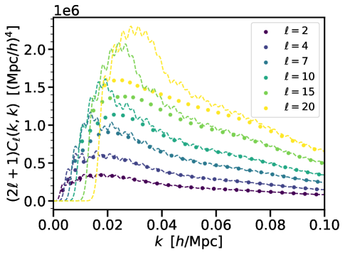
Figure 1: Comparing the continuous and discrete SFB power spectra for a uniform radial selection with a finite redshift range from $z_{\rm min}=0.2$ to $z_{\rm max}=0.5$. The points show the DSFB power spectrum, while the dashed lines show the CSFB. We assume the linear Newtonian RSD modeling in eq. 2.8 and $b_{1}=1.5$. Since it is impossible to properly normalize the CSFB basis in a finite volume, the CSFB and DSFB PS will not match in general. To roughly match the two spectra for comparison, we apply a single normalization factor to the continuous SFB PS at all $\ell$ and $k$. An additional $2(\ell+1)$ factor is applied on both the discrete and the continuous SFB PS to distinguish the different angular multipoles in the plot. We see that the DSFB spectrum is smooth and well-behaved since DSFB is a complete basis over the finite volume, while the CSFB spectrum suffers from oscillations due to the non-smoothness of the top-hat window in a finite redshift range.

In the case that the density volume reaches $x_{\rm min}=0$, the DSFB radial function is proportional to the continuous one at the discretized wavenumbers, that is $g_{n\ell}(x)=c_{n\ell}j_{\ell}(k_{n\ell}x)$, so the two power spectra will coincide up to some normalization. However, most tracers in realistic galaxy surveys start at some minimum redshift such that $x_{\rm min}(z_{\rm min})\neq 0$, in which case the DSFB radial basis function will become a generic linear combination of spherical Bessel functions of both first and second kinds as given in eq. 3.4, so the DSFB and CSFB spectra will become different. Assuming a finite redshift coverage from $z=0.2$ to $0.5$, we compare the CSFB and DSFB power spectra in figure 1, which are computed following section 4.2. Since the CSFB is not an orthonormal basis in a finite volume, it is hard to properly normalize the CSFB PS to exactly match the DSFB PS. We apply a single normalization factor to the continuous SFB PS at all $\ell$ and $k$ in figure 1 to roughly match the two spectra for comparison. We see that the discrete spectrum is smooth and well-behaved, while the CSFB spectrum suffers from oscillations due to the abrupt drop of galaxy density at the boundaries of the finite redshift range. Therefore, the DSFB PS is a more stable quantity when the redshift range starts at non-zero redshift.

Besides its numerical stability and aesthetic appeal, the DSFB basis has the theoretical advantage of being a complete basis of the density field over a finite volume. Discretisation imposes a discrete sampling of the SFB PS that can be efficiently represented in a matrix form $C_{\ell n_{1}n_{2}}\equiv C_{\ell}(k_{n_{1}\ell},k_{n_{2}\ell})$. For a Gaussian universe, the DSFB PS will contain all the information with a finite number of data points, serving as a lossless compression of the density field. For the CSFB, one has to choose a fine but arbitrary resolution in the Fourier $k$ modes during numerical computation, and results still need to be binned for practical purposes. In comparison, the DSFB naturally sets the $k$ resolution and avoids the arbitrary binning step. As seen in figure 1, there are only about 20 $k_{n\ell}$ modes in the linear regime ($k\lessapprox 0.1\,h/{\rm Mpc}$) for a full-sky volume from $z=0.2$ to $0.5$. Due to its efficient and complete decomposition of the field, the DSFB PS can be mapped to other two-point statistics, and the discrete basis simplifies and stabilizes the numerical implementation of these mappings as we will discuss in appendix A.

Furthermore, discretization explicits how the Fourier $k_{n\ell}$ modes depend on and vary with respect to angular multipoles $\ell$. For each angular mode $\ell$, DSFB naturally gives the lowest Fourier mode $k_{1\ell}$, representing the largest scale accessible at the given angular scale $\ell$. In general, only the largest angular scales at multipoles $\ell\lessapprox 10$ contribute to the lowest Fourier modes at $k\lessapprox 0.01\,h/{\rm Mpc}$, demonstrated in figure 1. Such explicit relationships between the angular and Fourier modes can help us better understand and control the various angular and redshift systematics in real surveys.

Besides the Fourier mode $k$ and angular multipole $\ell$, the DSFB basis also gives access to an additional index variable $n$, which does not exist for the CSFB. The exact meanings and applications of $n$ have not been extensively discussed, but in section 5.4 we will see that most of the lensing effect is contained in the $n=1$ modes, so these modes will be useful for measuring the lensing signal. We will also see that the index $n$ in the DSFB basis is somewhat analogous to the variable $\mu\equiv k_{||}/k$, parametrizing the component parallel to the LOS, often used in the plane-parallel limit. We expect $n$ to provide a useful handle for isolating different combinations of angular and radial modes in LSS surveys.

It is also more natural to use the DSFB basis to build estimators that can be applied to data, and a pseudo-$C_{\ell}$ estimator for the DSFB power spectrum has been fully developed in Ref. [33]. Therefore, the theoretical computation should match the DSFB estimator for validation and inference. For all these reasons, we recommend the use of the DSFB basis over the continuous one for numerical computation. In the rest of the paper, we simply use "SFB" to refer to the DSFB basis, and we will explicitly mention "continuous" when we refer to CSFB.

4 Computation of the SFB Power Spectrum

We now describe our method for computing the SFB power spectrum. We first summarize all the analytical formulas used for computing the SFB PS and GR effects in section 4.1, and we will develop some intuition based on these formulas. We next review the numerical approach proposed in Sec. IV of Ref. [35] for computing the SFB PS under the Newtonian RSD in section 4.2.1. We then adapt this approach to compute the GR effects in section 4.2.2.

4.1 Analytical Formalism

According to Refs. [34, 35], the SFB power spectrum given in eq. 3.8 can be computed using the following integral:

$$C_{\ell n_{1}n_{2}}^{\rm R} =\int_{0}^{\infty}dq\,\mathcal{W}_{n_{1}\ell}^{\rm R}(q)\mathcal{W}_{n_{2}\ell}^{\rm R}(q)P_{\rm m,0}(q)\,,$$ (4.1)

where $P_{\rm m,0}(q)$ is the present matter power spectrum under the comoving gauge, which can be computed from the linear Boltzmann codes. The SFB kernel $\mathcal{W}_{n\ell}(q)$ is given by

$$\mathcal{W}_{n\ell}^{\rm R}(q)\equiv\sqrt{\frac{2}{\pi}}q\int_{x_{\rm min}}^{x_{\rm max}}dx\,x^{2}g_{n\ell}(x)R(x)\Delta_{\ell}(x,q)\,.$$ (4.2)

We have added a radial selection function $R(x)$ to the SFB PS, and we use the subscript R to indicate this case. Here $\Delta_{\ell}(x,q)$ is the angular kernel that can contain various physical effects including the Newtonian RSD, GR effects [11, 12], redshift error modeling, and Fingers-of-god effects [34]. We will review the derivation of the above two formulas in section B.1.

To compute the GR effects in the SFB PS using eqs. 4.1 and 4.2, we summarize the angular kernels $\Delta_{\ell}(x,q)$ corresponding to all the linear-order GR effects (ignoring the observer’s terms) following Ref. [11, 12]:

$$\Delta_{\ell}(x,q)^{\rm DRSD}=b_{1}(x)D_{\rm m}(x,q)j_{\ell}(qx)+\frac{q}{\mathcal{H}(x)}v(x,q)j_{\ell}^{\prime\prime}(qx)$$ (4.3)

$$\Delta_{\ell}(x,q)^{\rm Doppler}=\mathcal{A}_{1}(x)v(x,q)j_{\ell}^{\prime}(qx)$$ (4.4)

$$\Delta_{\ell}(x,q)^{\rm NIP}=\Bigg{[}\left(\mathcal{A}_{1}(x)+1\right)\Psi(x,q)-(2-5s(x))\Phi(x,q)+\frac{1}{\mathcal{H}(x)}\dot{\Phi}(x,q)$$

$$\qquad\qquad\qquad+\left(b_{\rm e}(x)-3\right)\mathcal{H}(x)V(x,q)\Bigg{]}j_{\ell}(qx)$$ (4.5)

$$\Delta_{\ell}(x,q)^{\rm Lensing}=\ell(\ell+1)\frac{2-5s(x)}{2}\int_{0}^{x}dr\,\frac{x-r}{xr}(\Phi(r,q)+\Psi(r,q))j_{\ell}(qr)$$ (4.6)

$$\Delta_{\ell}(x,q)^{\rm Shapiro}=\frac{2-5s(x)}{x}\int_{0}^{x}dr\,(\Phi(r,q)+\Psi(r,q))j_{\ell}(qr)$$ (4.7)

$$\Delta_{\ell}(x,q)^{\rm ISW}=\mathcal{A}_{1}(x)\int_{0}^{x}dr\,\left(\dot{\Phi}(r,q)+\dot{\Psi}(r,q)\right)j_{\ell}(qr)\,.$$ (4.8)

Here $V(x(z),q)$ represents the transfer function for the velocity potential from the present-time matter perturbation $D_{{\rm m},0}(q)$; the same convention is followed for the transfer functions $\Phi(x,q)$ and $\Psi(x,q)$ for the two Bardeen potentials. These angular kernels have been given in Refs. [10, 11, 12] to compute the GR effects in the angular power spectrum, and they can be directly derived from the galaxy number count expression in eq. 2.3. For completeness, we will review the derivation of the above, as well as the angular kernels for the observer’s terms, in section B.2.

For a Universe with local non-Gaussian primordial fluctuations, an additional scale-dependent component to the angular kernel is added:

$$\Delta_{\ell}(x,q)^{\rm PNG}=\frac{f_{\rm NL}b_{\phi}(x)}{\alpha(q,x)}D_{\rm m}(x,q)j_{\ell}(qx).$$ (4.9)

The transfer functions for the velocity and gravitational potentials depend on the particular choice of cosmology, and in general they need to be calculated from the linear Boltzmann codes such as CAMB and CLASS. However, in the standard $\Lambda$CDM cosmology at the late time where one can ignore the anisotropic stress caused by radiation and neutrinos, the Friedmann equation and the linearized Einstein equations give the following [86, 17, 6]:

$$D_{\rm m}(x,q)=D(x)$$ (4.10)

$$v(x,q)=qV(x,q)=-f(x)\frac{\mathcal{H}(x)}{q}D(x)$$ (4.11)

$$\Phi(x,q)=\Psi(x,q)=-\frac{3}{2}\frac{\mathcal{H}^{2}(x)}{q^{2}}\Omega_{\rm m}(x)D(x)$$ (4.12)

$$\dot{\Phi}(x,q)=\dot{\Psi}(x,q)=-\frac{3}{2}\frac{\mathcal{H}^{3}(x)}{q^{2}}\Omega_{\rm m}(x)(f(x)-1)D(x)$$ (4.13)

$$\frac{\dot{\mathcal{H}}}{\mathcal{H}^{2}}=1-\frac{3}{2}\Omega_{\rm m}(x)\,,$$ (4.14)

where $D(x)$ is the linear growth factor normalized at the current time and $f(x)$ is the linear growth rate. In the $\Lambda$CDM model, the transfer functions are separable in terms of the conformal time indicated by the comoving distance $x(z)$ and the Fourier mode $k$. In this work, we will assume the $\Lambda$CDM model and use the above transfer functions to calculate the GR effects.

The above expressions for transfer functions directly indicate how individual GR effects scale with the Fourier mode as one moves closer to the horizon. The Doppler term is proportional to the velocity scalar $v$, which scales as $k^{-1}$ according to eq. 4.11. The GP term, including the NIP, Shapiro, and ISW effects, is proportional to the Bardeen potentials and their time derivative, which scale as $k^{-2}$ seen from eqs. 4.12 and 4.13. Proportional to the angular Laplacian of the Bardeen potentials, the lensing term will also scale as $k^{-2}$.

We can also predict the angular dependence of individual GR terms through the analytical formulas summarized in this section. Since the transfer functions do not contain any angular dependence, we see that there is no explicit dependence on $\ell$ besides the spherical Bessel function $j_{\ell}(qx)$ in the angular kernels for most GR terms. The exception is the lensing effect, which explicitly contains an $\ell(\ell+1)$ factor in its angular kernel given by eq. 4.6. We can therefore naively predict the lensing effect to scale as approximately $\ell^{2}$. These analytical predictions of dependence on $\ell$ and $k$ will be confirmed by the numerical results in section 5.1.

4.2 Numerical Computation

Our overall numerical strategy is to first integrate along $x$ to compute the SFB kernel in eq. 4.2 and then perform the integration along $q$ to obtain the SFB PS following eq. 4.1. This is also the integration order followed by previous SFB literature [25, 27, 28, 32, 34, 35], since eqs. 4.1 and 4.2 reduce the 3-dimensional (3D) integrals contained in the SFB PS to an effective 2D integral.

4.2.1 Summary of Iso-qr Integration

The main difficulty in computing the SFB power spectrum lies in the numerical evaluation of the SFB kernel $\mathcal{W}_{n\ell}(q)$. In the absence of GR effects with only the Newtonian RSD, Ref. [35] has proposed an efficient procedure to compute the SFB kernel such that the evaluation of the SFB power spectrum only takes seconds on a single CPU, enabling inference of cosmological parameters through MCMC with the SFB PS.

The key insight realized by Ref. [35] is that the bulk of the computation for the SFB kernel in eq. 4.2 is spent on evaluating the spherical Bessel functions $j_{\ell}(qx)$ inside the angular kernel $\Delta_{\ell}(x,q)$. We can put the formula for the SFB kernel into the general form of

$$\int_{x_{\rm min}}^{x_{\rm max}}dx\,f(x,q)j_{\ell}(qx)\,.$$ (4.15)

In the SFB kernel, the radial basis function $g_{n\ell}(x)$ will be precomputed, while the angular kernels $\Delta_{\ell}(x,q)$ for the DRSD term, as shown in eq. 4.3, only involves simple algebraic operations except the spherical Bessel functions $j_{\ell}(qx)$, so the evaluation of $f(x,q)$ is fast, while computing $j_{\ell}(qx)$ is slow.

Ref. [35] further notices that the spherical Bessel functions only depend on the variable combination $qx$, not on $q$ and $x$ separately. Thus, we can choose discretizations for $q$ and $x$ such that in q-x space the “iso-qx” lines go precisely through the grid points of $q$ and $x$. Using the “iso-qx” lines transforms the problem of calculating the spherical Bessel function from a 2D to a 1D problem: we can efficiently precompute and cache the values of spherical Bessel functions only on the “iso-qx” lines and then perform the 1D integration in eq. 4.15. We refer to this procedure as the Iso-qr integration. Ref. [35] has already given an outline of this algorithm, and we will supplement the details in appendix F and extend the algorithm to perform the Iso-qr integration over multiple subintervals in section F.5.

4.2.2 Adaptation for GR effects

The Iso-qr integration scheme has allowed the efficient computation of the SFB power spectrum under Newtonian RSD in Ref. [35]. In this work, we will use the same scheme extended for all the linear-order GR effects. The effects from eq. 4.3 to eq. 4.8 can be classified into two classes: the non-integrated terms and the integrated terms, the latter containing an extra integration along the LOS. The calculation of the SFB kernel $\mathcal{W}_{n\ell}(q)$ for the non-integrated terms can be directly achieved using the Iso-qr integration scheme without any modification: the standard Newtonian RSD term has already been implemented in Ref. [35], and the Doppler and NIP terms are simple extensions.

For the integrated terms including the lensing, Shapiro, and ISW terms (eqs. 4.8, 4.6 and 4.7), the SFB kernels contain an additional integration along the LOS in the angular kernel $\Delta_{\ell}(x,q)$. Fortunately, evaluating these integrated terms only requires small modifications to the Iso-qr integration method, which we will explain below.

To simplify the implementation, we first observe that the lensing term in eq. 4.6 can be written as a sum:

$$\Delta_{\ell}(x,q)^{\rm Lensing} =\left(\frac{2-5s(x)}{2}\right)\ell(\ell+1)\Bigg{[}\int_{0}^{x}dr\,\frac{1}{r}(\Phi(r,q)+\Psi(r,q))j_{\ell}(qr)$$

$$\qquad-\frac{1}{x}\int_{0}^{x}dr\,(\Phi(r,q)+\Psi(r,q))j_{\ell}(qr)\Bigg{]},$$ (4.16)

where the two integrands inside the integral along the LOS do not depend on the source redshift $x(z)$. The angular kernels of all three integrated terms can then be cast to the following form:

$$\Delta_{\ell}(x,q)^{\rm I} =K(x)\int_{0}^{x}dr\,g(r,q)j_{\ell}(qr)=K(x)\left[\int_{0}^{x_{\rm min}}dr\,g(r,q)j_{\ell}(qr)+\int_{x_{\rm min}}^{x}dr\,g(r,q)j_{\ell}(qr)\right]$$

$$=K(x)G(q)+\Delta_{\ell}(r=x_{\rm min}\to x,q)^{\rm I},$$ (4.17)

where we have split the LOS integral into two parts. The integration from $0$ to $x_{\rm min}$ does not depend on the source position $x$, so this part of the integral can be precomputed using the Iso-qr integration scheme over $0$ to $x_{\rm min}$ outside the SFB kernel evaluation loop and stored as an 1-D array $G(q)$.

We next examine the integration step from $x_{\rm min}$ to $x$. The SFB kernel in eq. 4.2 has the following form for the integrated terms (from $x_{\rm min}$ to $x$):

$$\mathcal{W}_{n_{1}\ell}^{\rm I}(q) \sim\int_{x_{\rm min}}^{x_{\rm max}}dx\,M(x)\int_{x_{\rm min}}^{x}dr\,g(r,q)j_{\ell}(qr)\,.$$ (4.18)

We can choose the outer integral and the inner integral in eq. 4.18 to share the same discretization scheme $\Delta x_{i}=\Delta r_{i}$ over the range $x_{\rm min}$ to $x_{\rm max}$ for the trapezoidal rule such that at a particular $q$:

$$\mathcal{W}_{n_{1}\ell}^{\rm I}(q)\sim\sum_{i=0}^{N}\Delta x_{i}\,M(x_{i})\sum_{j=0}^{i}\Delta r_{j}\,g(r_{j},q)j_{\ell}(qr_{j})\,.$$ (4.19)

Since the inner integrand in eq. 4.18 does not depend on $x$, the integration only needs to be performed for the outer integral, while we increment the inner integrand over the same interval as the following:

$$R_{i+1} \leftarrow R_{i}+\Delta x_{i}\,g(x_{i},q)j_{\ell}(qx_{i})\,,$$ (4.20)

$$\mathcal{W}_{n_{1}\ell}^{\rm I} \sim\sum_{i=0}^{N}\Delta x_{i}\,M(x_{i})R_{i}\,.$$ (4.21)

The above equations effectively rewrite eq. 4.19 into a weighted sum of a cumsum (cumulative sum), so the integrand only needs to be evaluated $N$ times where $N$ is the number of discretized bins from $x_{\rm min}$to $x_{\rm max}$. This reduces the 2D integral in eq. 4.18 to a 1-D summation, and one can obtain the discretization $\Delta x_{i}$ following the Iso-qr integration scheme to evaluate $j_{\ell}(qx)$.

Recall that the SFB kernel for the non-integrated terms has the form:

$$\mathcal{W}_{n_{1}\ell}^{\rm NI}(q) \sim\int_{x_{\rm min}}^{x_{\rm max}}dx\,f(x,q)j_{\ell}(qx)\,.$$ (4.22)

We can use the same "iso-qx" line from the Iso-qr integration scheme to evaluate the spherical Bessel functions for both non-integrated and integrated terms, since they cover the same range from $x_{\rm min}$ to $x_{\rm max}$. In summary, the computational complexity for the integrated terms remains the same order as the non-integrated terms. The integrated terms simply require an additional precomputation step to integrate from $0$ to $x_{\rm min}$ following eq. 4.17, and then increment the integrand following eq. 4.20 to integrate from $x_{\rm min}$ to $x_{\rm max}$.

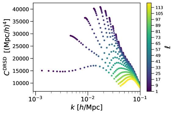
Figure 2: The DRSD (density plus RSD) term in the diagonal part of the SFB power spectrum $C_{\ell nn}\equiv C_{\ell}(k_{n\ell},k_{n\ell})$ for a redshift range from $z=1.0$ to $1.5$. The colormap shows the corresponding angular multipoles $\ell$. We only plot a subset of all the $\ell$ multipoles for visualization.

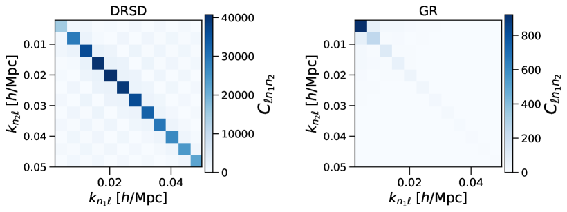
Figure 3: The full SFB power spectrum $C_{\ell n_{1}n_{2}}\equiv C_{\ell}(k_{n_{1}\ell},k_{n_{2}\ell})$ (including both the diagonal and off-diagonal parts) in $[{\rm Mpc}/h]^{4}$ at $\ell=3$ for a redshift range from $z=1.0$ to $1.5$. The left panel shows the DRSD term, while the right panel shows the total linear-order GR correction. With a uniform radial window, the SFB PS is mostly diagonal.

5 Results

Here we present our results of GR effects for SFB multipoles $\ell\geq 1$. We will discuss the SFB monopole in more detail in appendix E. Our numerical implementation has been validated by comparing the angular power spectra transformed from our SFB calculations using eq. A.7 and results directly obtained from CLASS, which we show in appendix C.

For all results in this section, we set the linear bias $b_{1}=1.5$, and we consider a vanishing magnification bias $s=0$ and evolution bias $b_{\rm e}=0$. Different values for the evolution and magnification biases will only change the amplitude of the GR corrections, and we do not expect our qualitative conclusions to change under other realistic values for these two biases. We assume the universal bias relation eq. 2.15 for any calculations related to the local PNG. We use the notation $C^{AB}$ to indicate the cross-correlation between the effects $A$ and $B$. The diagonal part of the SFB power spectrum $C_{\ell}(k_{n\ell},k_{n\ell})$ is the same regardless of the ordering of effects entering the cross-correlation, that is $C^{AB}$ and $C^{BA}$ have the same diagonal SFB PS. For reference, we show an example of the diagonal part of the SFB PS for the standard density plus the Newtonian RSD (DRSD) term in figure 2.

With the numerical formalism described in section 4.2, we can compute the full SFB power spectrum including both the diagonal ($n_{1}=n_{2}$) and the off-diagonal ($n_{1}\neq n_{2}$) terms. For a uniform radial function in the comoving space as we considered in this work, the off-diagonal terms are substantially smaller compared to the diagonal part of the spectrum for both the standard DRSD term and the total linear-order GR correction, as shown in figure 3. Therefore, we will focus our discussion on the diagonal terms in this work. With a non-uniform radial window as the case for real surveys, the diagonal part of the spectrum will then be mixed to the off-diagonal part, leading to more substantial contribution to the off-diagonal components [34, 35].

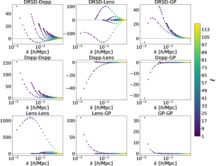
Figure 4: The GR terms in the diagonal part of the SFB power spectrum $C_{\ell nn}$ in $[{\rm Mpc}/h]^{4}$ for a redshift range from $z=1.0$ to $1.5$. The colormap shows the corresponding angular multipoles $\ell$. The thin grey lines indicate the $0$ value for the SFB PS. We only choose a subset of all the $\ell$ multipoles for visualization.

5.1 $\ell$ and $k$ Dependence

We first show the SFB PS for the auto-correlation and cross-correlation among all GR effects in figure 4 for a redshift range from $z=1.0$ to $1.5$ as an example. In general, GR corrections are only important at low Fourier modes corresponding to large scales, and all GR effects significantly decrease for higher $k$ values. The panels of figure 4 demonstrate the rich and different patterns of the individual GR terms in the SFB $\ell$-$k$ space. We next separately examine the $\ell$ and $k$ dependence of the GR terms in detail.

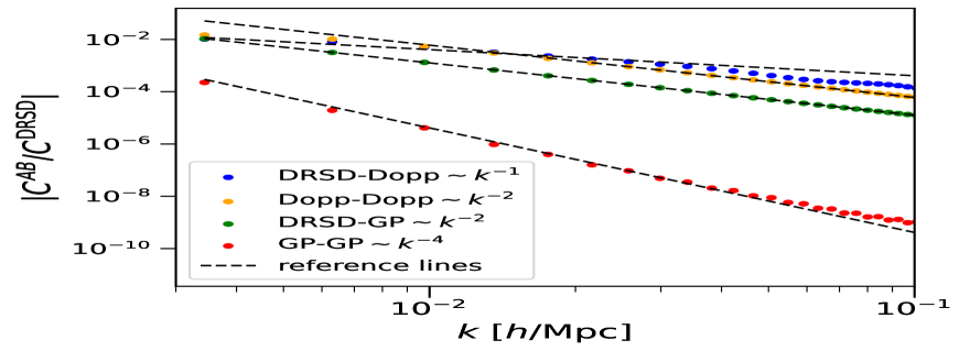
(a) $k$ dependence at $\ell=2$.

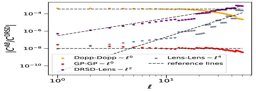
(b) $\ell$ dependence at $k\approx 0.04\,h/{\rm Mpc}$.

Figure 5: The $\ell$ and $k$ dependence of the diagonal part of the SFB PS $C_{\ell nn}$ for a redshift range from $z=0.2$ to $0.5$. We plot the absolute values of the ratios between the individual GR terms and the DRSD term. The dots represent the SFB PS, while the black dashed lines indicate the corresponding scaling behavior with respect to $k$ or $\ell$ respectively in the two subplots. Since the set of discrete Fourier modes $k_{n\ell}$ are different for each angular multipole, it is impossible to exactly fix the Fourier mode while varying $\ell$. To examine the angular dependence in the right subplot, we identify the $k_{n\ell}$ mode closest to $0.04\,h/{\rm Mpc}$ for each multipole $\ell$ as an approximation for fixing $k$. The inability of exactly fixing $k$ leads to some spurious oscillation patterns around the reference lines in the right subplot.

Fixing the angular multipole $\ell$, we show the scaling behaviors of the GR terms with the Fourier $k$ mode in figure 5(a), and they conform to our expectation based on the transfer functions given in eqs. 4.10, 4.11, 4.12 and 4.13. Proportional to the velocity scalar $v$, the DRSD-Doppler term scales roughly as $k^{-1}$ at large scales. In comparison, the DRSD-GP term scales almost exactly as $k^{-2}$ predicted by the transfer function for the potential $\Phi$. For the auto-correlation, the Doppler-Doppler and GP-GP terms scale as $k^{-2}$ and $k^{-4}$ respectively, in line with the k-scaling behavior for $v^{2}$ and $\Phi^{2}$. The lensing-lensing term also scales approximately as $k^{-4}$, seen in the right panel of figure 9 below, since it is also proportional to $\Phi^{2}$. Therefore, the Doppler effect has a shallower $k$ dependence compared to other GR effects, and it is the only GR effect proportional to the velocity field instead of the gravitational potential. Other cross-correlation GR terms such as Doppler-lensing, Doppler-GP, and lensing-GP terms shown in figure 4 also exhibit power-law scaling relation with $k$.

We next examine the angular dependence of the GR terms. The Doppler and GP terms do not exhibit any noticeable angular dependence as shown in figure 5(b). In contrast, the DRSD-lensing and lensing-lensing terms increase roughly as $\ell^{2}$ and $\ell^{4}$ as one considers larger angular multipoles $\ell$ corresponding to smaller angular scales. These scaling relationships can be fully explained by the $\ell(\ell+1)$ factor in the lensing angular kernel eq. 4.6. The angular Laplacian in the lensing convergence (eq. 2.4) imprints this unique angular dependence, setting lensing terms apart from all other linear-order GR terms. We will discuss more about lensing in section 5.4.

5.2 Evolution across Redshift

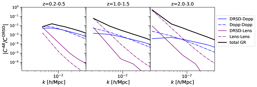
Figure 6: The importance of total and individual GR effects including Doppler and lensing terms in three redshift bins at $\ell=3$. Here we use lines instead of points to plot the discrete SFB PS to make the plots more readable. For the DRSD-lensing and lensing-lensing terms, we only plot the $k_{n\ell}$ modes where $n$ is odd to avoid showing the oscillations due to the parity of $n$, which can be seen in the figure 9 below.

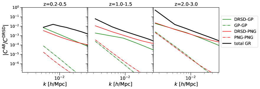
Figure 7: The importance of PNG and GP terms in three redshift bins at $\ell=3$. The PNG terms are computed assuming $f_{\rm NL}=1$.

We next discuss how GR terms evolve across the redshift. We show the relative significance of individual and total GR effects, normalized by the SFB PS under Newtonian DRSD, in three different redshift ranges in figures 6 and 7 at $\ell=3$. The total GR effect increases as one considers higher redshift: the GR correction is only around the percent level at the lowest redshift bin $z=0.2-0.5$, increasing to several percent for $z=1.0-1.5$, and reaching tens of percent for the high redshift bin $z=2.0-3.0$. This drastic increase in the significance of GR effects underlines the importance of modeling these terms for galaxy clustering at high redshift, which can be probed by the current Stage-IV and the proposed Stage-V surveys [87, 88, 89].

The increase of total GR effects at the high redshift is driven by the integrated terms including the lensing, Shapiro and ISW effects, which accumulate from the observer to the source along the LOS. Figures 6 and 7 show the increasing importance of lensing terms and GP terms respectively at higher redshift. Lensing terms become non-negligible for $z=1.0-1.5$, reaching a few percent at the lowest Fourier modes, and it drastically increases to tens of percent for $z=2.0-3.0$. In both redshift bins, the auto-correlation lensing-lensing term dominates over the cross-correlation DRSD-lensing term by about an order of magnitude. In comparison, the cross-correlation DRSD-GP term dominates over the auto-correlation GP-GP term as seen in figure 7. The RSD-GP term remains at the sub-percent level for the two lower redshift bins, and it increases above the percent level for the highest redshift bin $z=2.0-3.0$.

While the lensing and GP effect increase at higher redshift, the Doppler effect gradually decreases in significance as seen in figure 6. The Doppler effect, including the cross-correlation DRSD-Doppler term and the auto-correlation Doppler-Doppler term, is the dominant GR correction at the lowest redshift bin $z=0.2-0.5$, reaching the percent level, but it becomes negligible compared to other GR effects at the highest redshift bin $z=2.0-3.0$. In summary, the Doppler effect is important at low redshift, while lensing is dominant at high redshift. The redshift evolution pattern we observe in the SFB space is qualitatively in agreement with previous literature such as Refs. [10, 11, 90] and [17] that examine the individual GR effects in TSH and PSM respectively.

5.3 Degeneracy with PNG

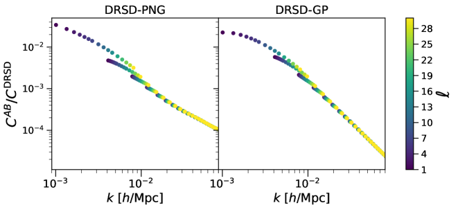
Figure 8: Comparison between the DRSD-PNG and DRSD-GP terms, normalized by the Newtonian DRSD term, in $C_{\ell nn}$ for $z=2.0$ to $3.0$. The DRSD-PNG term is calculated with $f_{\rm NL}=1$. We only show the SFB modes with low $\ell$ values for clarity, and the decreasing trend continues for higher $\ell$ multipoles.

During our review of the local PNG in section 2.2, we discussed the possible degeneracy between the GP and PNG terms, since both effects are directly proportional to the gravitational potential $\Phi$. We now compare our numerical results for the DRSD-GP term and the DRSD-PNG term, which is evaluated at $f_{\rm NL}=1$, in the SFB space in figure 8. We see that these two effects have almost the same dependence on $\ell$ and $k$, implying the degeneracy between the two signals. However, these two effects evolve slightly differently across the redshift, since the PNG effect depends on the potential during the matter-dominated era, while the GP effect contains the NIP term (depending on $\Phi$ at the source), the Shapiro term (depending on $\Phi$ integrated along the LOS), and the ISW term (depending on $\dot{\Phi}$ integrated along the LOS). In figure 7, we see that the GP effect mimics a local PNG signal of unity for the redshift bin $z=2.0-3.0$, and it becomes slightly larger and smaller than $f_{\rm NL}\sim 1$ for $z=0.2-0.5$ and $1.0-1.5$ respectively. In general, the GP effect mimics $f_{\rm NL}\sim\mathcal{O}(1)$, so it will be important to model the GP effect for surveys aiming to constraint $\sigma(f_{\rm NL})\sim 1$ so as to avoid any bias in the measurement.

Even though the GP effect is degenerate with the local PNG, the Doppler and lensing effects do not exhibit the same degeneracy, since the Doppler effect has a distinct $k$-dependence, while the lensing effect has a unique $\ell$-dependence as previously discussed. Therefore, the total GR effects are not completely degenerate with $f_{\rm NL}$ in the SFB space. However, to achieve consistency in modeling, GR effects should be considered for surveys reaching $\sigma(f_{\rm NL})$ to a few, since the total GR effect is noticeably larger than the local PNG effect at $f_{\rm NL}=1$ across the redshift as illustrated in figure 7.

5.4 Behavior of Lensing

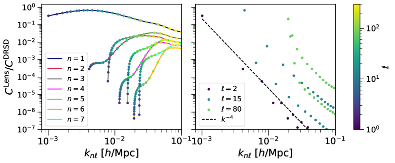
Figure 9: The behavior of the lensing-lensing term for $C_{\ell nn}$, normalized by the SFB PS under the Newtonian DRSD term, for a redshift range from $z=2.0$ to $3.0$. The dots show the values of the SFB PS, with the angular modes indicated by the colormap. The left panel emphasizes the dependence of the lensing effect on $n$, and we use color dashed lines to connect the Fourier modes $k_{n\ell}$ with the same $n$. The dots only show a subset of all the $\ell$ multipoles at each $n$ for visualization. In the right panel, we plot the lensing effect at several particular angular multipoles $\ell$ to show the $k$-dependence.

We next focus on the behavior of the lensing-lensing term, since it is the most important correction at $z\gtrapprox 1$ as demonstrated in figures 4 and 6, dominating over other GR corrections by at an order of magnitude. The lower left panel of figure 4 singles out one prominent branch of the SFB PS compared to other SFB modes. Further examination in the left panel of figure 9 shows that this dominant branch in the lensing-lensing term corresponds to the SFB $k_{n\ell}$ modes with varying $\ell$ at the constant $n=1$. These $k_{1\ell}$ modes correspond to the largest scale (the lowest Fourier mode) accessible at each angular multipole.

The left panel of figure 9 shows the prominent dependence of the lensing term on $n$. For a fixed $n$, the lensing effect remains relatively stable for smaller angular scales. On the iso-$n$ contour of an approximately horizontal direction, smaller Fourier scales (higher $k$ values) correspond to smaller angular scales (higher $\ell$ values), and the $\ell(\ell+1)$ factor imprinted by the angular Laplacian compensates the $k^{-2}$ scaling behavior in the potential $\Phi$ and $\Psi$, resulting in a relatively stable lensing correction even for smaller angular scales.

Fixing the Fourier mode $k$, we see that the lensing correction drastically decreases for higher $n$ values as seen in the left panel of figure 9. This is because a higher $n$ mode on the iso-$k$ contour corresponds to a lower $\ell$ value (larger angular scales), which dramatically suppresses the lensing-lensing correction due to its approximate $\ell^{4}$ dependence. This explains the dominance of the $n=1$ branch, since it has the highest $\ell$ mode for a given $k$.

In the plane-parallel limit, the transverse Fourier mode can be approximated by $k_{\perp}\approx\ell/r_{\rm eff}$ for a given angular multipole $\ell$, where $r_{\rm eff}$ is the effective comoving distance for a relatively narrow redshift bin, and the parallel Fourier mode can be given by $k_{||}^{2}=k_{n\ell}^{2}-k_{\perp}^{2}$. Therefore, higher angular multipoles correspond to higher $k_{\perp}$ values and smaller transverse scales. On the iso-$k$ contour (the vertical directions in figure 9), smaller $n$ values correspond to higher $\ell$ values and lower $k_{||}$ values, which represent larger radial scales. Therefore, the $n=1$ branch represents the largest radial scales accessible at each $\ell$ and the smallest angular scales accessible at each $k$. In the plane-parallel language, $n=1$ can then be approximately characterized as $\mu\equiv k_{||}/k\approx 0$, where lensing is the most dominant.

Interestingly, there seems to be some parity dependence on $n$ for the lensing correction. Examining the left panel of figure 9, we see that the branches with the same parity of $n$ (except the dominant $n=1$ branch) demonstrate similar patterns. The lensing correction only strictly decreases for increasing $n$ values of the same parity, while the neighboring branches, such as $n=2$ and $3$ branches can intersect each other. This parity dependence can also be seen in the iso-$\ell$ contour plotted in the right subplot of figure 9, where there are two distinct lines decreasing with higher $k$ for a fixed $\ell$.

The lensing pattern we see in the SFB space is consistent with previous works that examine the lensing effect in PSM and TSH. Refs. [17, 6] shows the lensing PSM $P_{L}(k)$ drastically decreases for higher $k$ values, while the lensing correction roughly remains stable in significance as $\ell$ increases as seen in Refs. [10, 11] for the TSH case. The angular power spectrum sums over all Fourier modes $n$ (as explicitly shown in eq. A.7), so the lensing correction in the TSH will be dominated by the $n=1$ branch. The relative stability of the $n=1$ branch explains the stability of the lensing effect with respect to $\ell$ in the TSH. Therefore, the SFB PS demonstrates the same $\ell$ and $k$ dependence for lensing as in previous works. The clear separation of the radial and angular scales in the SFB basis allows us to examine both sets of dependence at the same time and fully captures the rich pattern of the lensing convergence.

Last, we highlight the exciting opportunity of measuring the lensing convergence present in the galaxy clustering at high redshift through the SFB basis. Figure 9 shows the lensing correction reaches tens of percent of the Newtonian DRSD clustering in the $k_{1\ell}$ modes across a wide range of $\ell$ at the redshift bin $z=2.0-3.0$. These $n=1$ modes capture most of the lensing effect compared to the higher $n$ modes. Since the lensing effect becomes comparable to the density plus Newtonian RSD term, it will become measurable at these $n=1$ modes. Therefore, it is important to model the lensing effect for the future Stage-V galaxy surveys aiming at the high redshift Universe for both achieving precise cosmological constraints and measuring the lensing convergence.

6 Conclusion and Discussion

As the current and upcoming LSS surveys probe galaxy clustering over increasingly large volumes, the spherical Fourier-Bessel basis provides a powerful tool to model the general relativistic and wide-angle effects that become important at large scales. In this paper, we presented the first computation of the linear-order relativistic effects in the discrete SFB power spectrum. Compared to the continuous SFB basis used in previous works [25, 37] for modeling GR effects, the discrete basis we adopt here provides a more stable and efficient decomposition of the galaxy density field and matches the implementation of estimators. Our main numerical approach is based on the Iso-qr integration scheme introduced in Ref. [35], and we have adapted the method for the integrated GR terms including the lensing, Shapiro, and ISW effects. Moreover, we have validated our implementation of GR effects by transforming our SFB PS results to the TSH (through the mapping in eq. A.7), which agree well with outputs from CLASS.

The SFB basis has allowed us to examine both angular $\ell$ and Fourier mode $k$ dependence of the GR effects at the same time, and we find that the Doppler effect has a shallower $k$ dependence compared to other GR effects, while the lensing effect has a unique $\ell$ dependence due to the angular Laplacian in the lensing convergence. The effect of local primordial non-Gaussianities shares similar pattern in the $\ell$-$k$ space with the gravitational potential term, suggesting degeneracy between the two and the need of modeling the GP term when $\sigma(f_{\rm NL})\sim 1$ is reached. The Doppler effect is the most important at the low redshift, while the lensing convergence dominates at the high redshift. Due to the large impacts of the lensing effect on the $k_{n\ell}$ modes with $n=1$ (which correspond to the largest scales at each angular multipole) at the high redshift, upcoming LSS surveys can potentially measure the lensing convergence present in galaxy clustering by measuring these SFB modes. In general, GR effects become increasingly important at higher redshift, and these effects should be considered when we can constraint $f_{\rm NL}$ to a few.

We have so far considered all linear-order GR effects in the SFB space, except the observer’s terms. Considering a full-sky survey with no angular mask, the observer’s potential only impacts the SFB monopole, while the observer’s velocity only impacts the SFB dipole (as shown in section B.2.1). For cosmological inference with the SFB PS, one can simply exclude the first two multipoles and use angular modes $\ell\geq 2$ similar to the CMB analysis [43]. Therefore, the observer’s terms are of no concern for the main cosmological analysis of galaxy surveys.

However, they are still interesting quantities for both theory and observation. The observer’s potential is instrumental for the cancellation of infrared divergence in the GR effects at the SFB monopole, which we will discuss more in appendix E. The presence of the observer’s velocity in the dipole offers the opportunity to test the cosmological principle in the SFB basis. The observer’s velocity, which is our kinematic velocity with respect to the CMB rest frame and also more commonly known as the kinematic dipole, has been measured from LSS tracers such as quasars [91, 92] or radio sources [93, 94] using the projected statistics purely in the angular space. These measurements from LSS are in various degrees of tension with respect to the CMB measurement [95, 96, 97, 98, 99, 100]. Compared to the projected statistics in the angular space, the SFB basis contains the full 3D information and offers a better handle on systematics, so it provides another promising avenue for measuring the kinematic dipole. We will discuss all these issues related to the observer’s terms in depth in forthcoming works.

We emphasize that our calculation of the relativistic effect is performed under the strict assumption of the standard $\Lambda$CDM model under General Relativity. Ref. [101] has explored modified gravity models in the SFB basis, albeit with the Newtonian modeling of RSD. To extend our calculation of general relativistic SFB to non-$\Lambda$CDM models, one has to obtain the transfer functions $V(z,k)$, $\Psi(z,k)$ and $\Phi(z,k)$ from modified Boltzmann models such as MGCAMB [102], EFTCAMB [103], and hiclass [104]. All numerical techniques used in this work remain effective under relatively smooth velocity and potential transfer functions, and we did not assume the separability between the redshift evolution $z$ and the Fourier mode $k$ in these transfer functions. Therefore, to extend our calculation of the relativistic effects to non-$\Lambda$CDM models, we will only need to integrate our SFB implementation with a Boltzmann code. Such an implementation will allow a rigorous test of modified gravity or alternative dark energy theories at the perturbation level with galaxy clustering on the largest scales, similar to how the low-$\ell$ part of the CMB power spectra provide constraints on these non-$\Lambda$CDM models at the perturbation level [105, 43].

Assuming the standard $\Lambda$CDM model under GR, our validated calculation of the linear-order relativistic correction in the SFB PS can be used for the cosmological analysis of large-scale clustering. However, further optimization and computation speedup will be required to use our calculation for MCMC inference. With the Iso-qr integration scheme, we can compute the SFB power spectrum including all GR effects in a couple of seconds with a single CPU, for a lower redshift bin $z\lesssim 0.5$ considering all the radial Fourier modes $k_{n\ell}\lesssim 0.1h/{\rm Mpc}$. However, the computation can take tens of seconds when one considers higher redshift or smaller scales. As suggested in Ref. [32], further computation speedup on evaluating the SFB PS might be achieved by using a FFTLog-based method similar to Refs. [106, 107, 13, 61] for the angular power spectrum. Our Iso-qr integration scheme has the advantage of not requiring the potential transfer functions including $V(z,k)$ and $\Phi(z,k)$ to be separable, and it does not require apodization and zero-padding schemes employed in FFTLog. Our implementation can serve as the baseline for a more optimized implementation of the SFB PS in the future.

Our calculation of GR effects in the SFB PS will also have implications for the modeling of GR effects in other two-point statistics, since the SFB basis is a complete decomposition of the Gaussian density field and can be transformed into other statistics (as shown in appendix A). In particular, we will be able to use the SFB-to-PSM mappping introduced and developed by Refs. [21, 23, 108] to calculate the GR effects present in the PSM, which has been the preferred statistics for Fourier-space clustering analysis due to the efficient implementation of its estimator, efficient representation of RSD effects, and well-developed non-linear scale modeling. We will also be able to compute the PSM covariance with GR effects using the mapping between the PSM covariance and SFB PS introduced in Ref. [23], which will then allow us to forecast the measurability of GR effects and assess their impact on the $f_{\rm NL}$ constraints from PSM for future surveys. Our theoretical modeling of linear-order GR effects in the SFB basis will play an important role to the analysis of the large-scale clustering to be measured in the upcoming LSS surveys.

Our work can be extended to the SFB bispectrum, of which the numerical evaluation is recently achieved in Ref. [36] under Newtonian RSD. Modeling GR effects for the SFB bispectrum is significantly more challenging than the power spectrum case due to the very large number of terms present in the second-order GR effects [49, 109, 110, 111, 112] and the higher dimensions of the integrals, but they can be important for the upcoming LSS surveys such as SPHEREx aiming at achieving $\sigma(f_{\rm NL})\sim 0.5$ through the bispectrum analysis [6]. Our work lays out the foundation for future works investigating higher-order GR effects in the discrete SFB basis, which will help us to fully utilize the cosmological information and probe fundamental physics at the largest scales in the observable Universe.

Appendix A Mapping with SFB

Since the SFB basis is a complete decomposition of the density field, one can express any other two-point statistics in terms of the SFB power spectrum. We will first give the mappings between the angular power spectrum and the SFB PS in section A.1. These mappings will be helpful for deriving the SFB kernels in section B.1 and validating our GR results in appendix C. The mapping from the SFB PS to TSH can be further extended to the projected angular power spectrum and the correlation function multipoles $\xi_{L}(s,x)$, which we give in section A.2 and section A.3 respectively. The mapping from the SFB power spectrum to the power spectrum multipoles (PSM) was first given in Ref. [21, 23] for the continuous SFB basis and then in Ref. [108] for the discrete case. This section will complete the study of transforming the SFB PS to other common two-point statistics used in galaxy surveys.

A.1 TSH-SFB Mapping

As seen in eqs. 3.1 and 3.6, the SFB transform relies on the spherical harmonics to obtain the angular modes. Angular multipoles $\ell$ are typically encountered in the context of the angular power spectrum. In fact, the angular $\ell$ modes share the same physical interpretation for both TSH and SFB, which we will demonstrate by giving the mappings between TSH and SFB.

The spherical harmonic mode $\delta_{\ell m}(x(z))$ in the configuration space is defined as

$$\delta_{\ell m}(x)=\int_{\hat{\mathbf{n}}}Y^{*}_{\ell m}(\hat{\mathbf{n}})\delta(\mathbf{x}).$$ (A.1)

These spherical harmonic modes form the angular power spectrum:

$$\langle\delta_{\ell_{1}m_{1}}(x)\delta_{\ell_{2}m_{2}}(x^{\prime})\rangle=C_{\ell_{1}}(x,x^{\prime})\delta^{K}_{\ell_{1}\ell_{2}}\delta^{K}_{m_{1}m_{2}},$$ (A.2)

and it is more conventional to directly write the angular power spectrum in terms of the redshift $C_{\ell}(z,z^{\prime})$ instead of the comoving distance.

We now observe the relationship between the SFB mode $\delta_{n\ell m}$ and the TSH mode $\delta_{\ell m}(x)$. From the definition of the SFB mode in eq. 3.6, we have

$$\delta_{n\ell m} =\int_{x_{\rm min}}^{x_{\rm max}}dx\,x^{2}g_{n\ell}(x)\int_{\hat{\mathbf{n}}}Y^{*}_{\ell m}(\hat{\mathbf{n}})\delta(\mathbf{x})=\int_{x_{\rm min}}^{x_{\rm max}}dx\,x^{2}g_{n\ell}(x)\delta_{\ell m}(x).$$ (A.3)

Therefore, the SFB power spectrum can be written as a two-dimensional integral transform of the angular power spectrum:

$$C_{\ell n_{1}n_{2}} =\int_{x_{\rm min}}^{x_{\rm max}}dx\,x^{2}g_{n_{1}\ell}(x)\int_{x_{\rm min}}^{x_{\rm max}}dx^{\prime}\,x^{\prime 2}g_{n_{2}\ell}(x^{\prime})C_{\ell}(x,x^{\prime})\,$$ (A.4)

which maps the TSH to the SFB space. The SFB PS and TSH that entered the above equation share the same value of $\ell$, and both statistics reside in the same angular space.

The above eq. A.4 assumes a uniform selection in the comoving space within the redshift range. To include a radial selection function $R(x)$ in the SFB power spectrum (we use the superscript R to indicate this case), we can generalize eq. A.4 to obtain:

$$C_{\ell n_{1}n_{2}}^{\rm R} =\int_{x_{\rm min}}^{x_{\rm max}}dx\,x^{2}g_{n_{1}\ell}(x)R(x)\int_{x_{\rm min}}^{x_{\rm max}}dx^{\prime}\,x^{\prime 2}g_{n_{2}\ell}(x^{\prime})R(x^{\prime})C_{\ell}(x,x^{\prime})\,.$$ (A.5)

Our SFB calculation in section 4 is formulated for the above case with the presence of a radial selection function.

Since the numerical computation of the angular power spectrum has been extensively developed in literature [113, 107, 106, 114, 61, 115], with the linear-order GR effects included in Refs. [10, 12, 13], eq. A.5 raises the interesting question of whether it is possible to calculate the SFB PS relying on existing implementations of the TSH instead of using the SFB kernel as we did in section 4. The main challenge of directly using the TSH-to-SFB map in eq. A.4 for numerical evaluations is the non-trivial 2D integration of the angular power spectrum, and the total integration involved in evaluating the SFB PS will remain 3D. In contrast, using the SFB kernel in eq. 4.2 and calculating the SFB PS with eq. 4.1 effectively reduce the integral to 2D, which renders the computation more tractable.

We next show the inverse transform that maps the SFB back to the TSH space. Substituting eq. 3.7 into eq. A.1, we have:

$$\delta_{\ell m}(x) =\int_{\hat{\mathbf{n}}}Y_{\ell m}^{*}(\hat{\mathbf{n}})\sum_{n\ell^{\prime}m^{\prime}}g_{n\ell^{\prime}}(x)Y_{\ell^{\prime}m^{\prime}}(\hat{\mathbf{n}})\delta_{n\ell^{\prime}m^{\prime}}=\sum_{n}g_{n\ell}(x)\delta_{n\ell m}\,,$$ (A.6)

where we applied the orthogonality of the spherical harmonics in eq. G.1. The angular power spectrum defined in eq. A.2 is then related to the SFB power spectrum defined in eq. 3.8 through:

$$C_{\ell}(x,x^{\prime})=\sum_{n_{1},n_{2}}g_{n_{1}\ell}(x)g_{n_{2}\ell}(x^{\prime})C_{\ell n_{1}n_{2}}\,,$$ (A.7)

where the TSH sums over the Fourier modes present in the SFB.

According to eq. A.7, it is theoretically possible to calculate an arbitrary angular power spectrum through the SFB power spectrum when $x$ and $x^{\prime}$ are within the radial range considered for the SFB PS. In reality, however, eq. A.7 is difficult to use for computing the density and Newtonian RSD terms, since they do not decrease for smaller Fourier scales (as seen in figure 2), which necessitates the inclusion of many $n_{1}$ and $n_{2}$ terms to account for higher $k_{n\ell}$ modes. The computational complexity of the SFB PS generally scales with $k_{\rm max}^{3}$, making it expensive to evaluate for smaller Fourier scales, so the mapping is difficult to use for the DRSD term. Fortunately, all GR terms substantially decrease when the Fourier mode $k_{n\ell}$ increases, as we discussed in section 5. As a result, computing GR effects in TSH through eq. A.7 only requires the inclusion of the SFB PS at lower Fourier modes, and we can obtain accurate results of GR effects in TSH at lower angular multipoles. This map from the SFB PS to TSH will be instrumental for validating our GR calculations in appendix C.

In addition to computing TSH through SFB, eq. A.7 also offers a clear indication where the TSH needs non-linear modeling, since the expression explicitly gives which Fourier $k_{nl}$ modes are folded into the TSH. For realistic galaxy surveys, it is impossible to estimate the TSH between arbitrary redshift pairs. One instead estimate a projected version of TSH (pTSH) where the 3-D galaxy field is projected along the radial direction within some redshift bin. We give and discuss the mapping from SFB to pTSH in section A.2.

To our knowledge, our work represents the first time a mapping from the discrete SFB power spectrum to TSH is explicitly written down and used for numerical calculations. An analog to eq. A.7 that maps the continuous SFB power spectrum to TSH can be similarly derived by substituting eq. 3.2 into eq. A.1:

$$C_{\ell}(x,x^{\prime})=\frac{4}{\pi^{2}}\int_{0}^{\infty}dk_{1}\,\int_{0}^{\infty}dk_{2}\,k_{1}^{2}k_{2}^{2}j_{\ell}(k_{1}x)j_{\ell}(k_{2}x^{\prime})C_{\ell}(k_{1},k_{2})\,.$$ (A.8)

However, it is significantly harder to apply the continuous version in eq. A.8, since one needs fine resolution of $k$ modes to perform integration over all positive $k$ values, while in the discrete case of eq. A.7, the integration reduces to a sum over well-defined discrete $k_{nl}$ modes. This suggests another advantage of the discrete SFB basis: the transformations from the discrete SFB PS to other two-point statistics have relatively simple, stable numerical implementations.

A.2 SFB-to-pTSH Mapping

We next consider the radially-integrated angular power spectrum, which we also refer to as the projected tomographic spherical harmonic (pTSH). Using the relationship between the spherical harmonic mode $\delta_{\ell m}(x)$ and the SFB mode $\delta_{n\ell m}$ of the unprojected density field in eq. A.6, we have

$$\delta_{\ell m} =\int_{x_{\rm min}}^{x_{\rm max}}dx\,x^{2}\delta_{\ell m}(x)=\sum_{n}\left[\int_{x_{\rm min}}^{x_{\rm max}}dx\,x^{2}g_{n\ell}(x)\right]\delta_{n\ell m}=\sum_{n}b_{n\ell}\delta_{n\ell m},$$ (A.9)

where $b_{n\ell}=\int_{x_{\rm min}}^{x_{\rm max}}dx\,x^{2}g_{n\ell}(x)$. Therefore, the pTSH is related to the SFB PS as the following:

$$C_{\ell}=\sum_{n,n^{\prime}}b_{n\ell}b_{n^{\prime}\ell}C_{\ell nn^{\prime}}\,.$$ (A.10)

The above equation is the extension of eq. A.7 for the projected angular power spectrum measured in real surveys. This mapping can help to establish consistency between the SFB PS and pTSH measurements and explicitly show the exact radial Fourier modes being included at each angular multipole for a projected measurement.

A.3 SFB-to-2CF Mapping

We now build upon eq. A.7 to obtain the mapping from the SFB PS to the two-point correlation function $\langle\delta(\mathbf{x})\delta(\mathbf{x}^{\prime})\rangle$. It is well-known that the two-point correlation function can be expanded with Legendre polynomials into the angular power spectrum [12, 32]:

$$\langle\delta(\mathbf{x})\delta(\mathbf{x}^{\prime})\rangle=\frac{1}{4\pi}\sum_{\ell}(2\ell+1)C_{\ell}(x,x^{\prime})\mathcal{L}_{\ell}(\hat{\mathbf{n}}\cdot\hat{\mathbf{n}}^{\prime})\,.$$ (A.11)

Substituting eq. A.7 into eq. A.11, we have:

$$\langle\delta(\mathbf{x})\delta(\mathbf{x}^{\prime})\rangle=\frac{1}{4\pi}\sum_{\ell,n_{1},n_{2}}(2\ell+1)\mathcal{L}_{\ell}(\hat{\mathbf{n}}\cdot\hat{\mathbf{n}}^{\prime})g_{n_{1}\ell}(x)g_{n_{2}\ell}(x^{\prime})C_{\ell n_{1}n_{2}},$$ (A.12)

which can also be derived directly from eq. 3.7.

The above mapping can be useful for developing an optimal quadratic estimator for the SFB PS at the ultra-large scales. The existing estimator for the SFB PS developed in Ref. [33] is based on the pseudo-$C_{\ell}$ approach [116, 117], which performs well for small angular scales but becomes non-optimal for the largest angular scales. The optimal quadratic estimator requires knowing the covariance between any two galaxy positions (or pixels) and the derivative of the covariance with respect to the band-powers [118, 119]. Equation A.12 directly expresses the covariance between any two galaxy positions (the correlation function) in terms of the band-powers (the SFB PS), so it can be used for building a quadratic estimator for the SFB PS.

The correlation function can be reparametrized in terms of the relative displacement $\mathbf{s}=\mathbf{x}-\mathbf{x}^{\prime}$ between the two galaxies:

$$\xi(s,x,\hat{\mathbf{n}}\cdot\hat{\mathbf{s}})=\xi(\mathbf{s},\mathbf{x})\equiv\langle\delta(\mathbf{x})\delta(\mathbf{x}-\mathbf{s})\rangle\,.$$ (A.13)

It can then be decomposed with respect to $\mu\equiv\hat{\mathbf{n}}\cdot\hat{\mathbf{s}}$ to obtain the the two-point correlation function multipoles (2CFM) under the end-point LOS:

$$\xi_{L}(s,x)\equiv\frac{2L+1}{2}\int_{\mu=-1}^{1}\mathcal{L}_{L}(\mu)\xi(s,x,\mu)\,,$$ (A.14)

which are frequently used in the analysis of spectroscopic surveys.

One can then express the 2CFM as a map from the SFB PS:

$$\xi_{L}(s,x)\equiv\frac{2L+1}{8\pi}\sum_{\ell,n_{1},n_{2}}(2\ell+1)g_{n_{1}\ell}(x)C_{\ell n_{1}n_{2}}S_{n_{2}\ell}^{L}\,,$$ (A.15)

where

$$S_{n_{2}\ell}^{L}\equiv\int_{\mu=-1}^{1}\mathcal{L}_{L}(\mu)\mathcal{L}_{\ell}(\hat{\mathbf{n}}\cdot\hat{\mathbf{n}}^{\prime})g_{n_{2}\ell}(x^{\prime}=\sqrt{x^{2}+s^{2}-2xs\mu})\,.$$ (A.16)

Therefore, another possible validation route for the SFB calculation performed in this work is to compare the 2CFM results transformed from our SFB calculation with existing codes COFFE [18] or GaPSE [7] that can calculate the GR effects in the configuration-space 2CFM. However, the mapping from the SFB PS to the 2CFM in eq. A.15 is more complicated than the SFB-to-TSH map in eq. A.7. In addition, CLASS is a more established and validated cosmological code, with two independent methods implemented for calculating the GR effects in TSH [12, 13]. Therefore, we choose the TSH over the 2CFM for validation in this work.

Appendix B Spherical Harmonic Decomposition

B.1 SFB Kernels

In this appendix, we will derive eqs. 4.1 and 4.2 that are used to compute the SFB power spectrum. Our derivation will rely on the TSH-to-SFB mapping given in eq. A.4.

Suppose we can write the spherical harmonic mode of the observed galaxy density in the following form:

$$\delta_{\ell m}(x) =\frac{1}{2\pi^{2}}i^{\ell}\int_{\mathbf{q}}\Delta_{\ell}(x,q)D_{\rm m,0}(\mathbf{q})Y_{\ell m}^{*}(\hat{\mathbf{q}}),$$ (B.1)

where $\Delta_{\ell}(x,q)$ is the angular kernel and $D_{{\rm m},0}$ is the comoving matter density at the present time. We will show in the following section that all GR effects can indeed be expressed into the above form in terms of some angular kernels. The angular power spectrum (TSH) defined in eq. A.2 becomes:

$$\langle\delta_{\ell m}(x)\delta_{\ell^{\prime}m^{\prime}}^{*}(x^{\prime})\rangle =\frac{1}{4\pi^{4}}i^{\ell-\ell^{\prime}}\int_{\mathbf{q}}\Delta_{\ell}(x,q)Y_{\ell m}^{*}(\hat{\mathbf{q}})\int_{\mathbf{q}^{\prime}}\Delta_{\ell}(x^{\prime},q^{\prime})Y_{\ell^{\prime}m^{\prime}}(\hat{\mathbf{q}}^{\prime})\langle D_{\rm m,0}(\mathbf{q})D_{\rm m,0}(\mathbf{q}^{\prime})\rangle\,.$$ (B.2)

The translational invariance and the statistical isotropy of the universe for the matter distribution imply that

$$\langle D_{\rm m,0}(\mathbf{q})D_{\rm m,0}(\mathbf{q}^{\prime})\rangle=(2\pi)^{3}\delta(\mathbf{q}-\mathbf{q}^{\prime})P_{\rm m,0}(q),$$ (B.3)

where $P_{\rm m,0}(q)$ is the matter power spectrum at the present time. Substituting the above matter power spectra into eq. B.2, we have

$$C_{\ell}(x(z),x^{\prime}(z^{\prime})) =\frac{2}{\pi}\int_{0}^{\infty}dq\,q^{2}\Delta_{\ell}(x,q)\Delta_{\ell}(x^{\prime},q)P_{\rm m,0}(q)i^{\ell-\ell^{\prime}}\int_{\hat{\mathbf{q}}}Y_{\ell m}^{*}(\hat{\mathbf{q}})Y_{\ell^{\prime}m^{\prime}}(\hat{\mathbf{q}})\,.$$ (B.4)

We then use the orthogonality of the spherical Harmonics in eq. G.1 to obtain:

$$C_{\ell}(x,x^{\prime})=\frac{2}{\pi}\int_{0}^{\infty}dq\,q^{2}P_{\rm m,0}(q)\Delta_{\ell}(x,q)\Delta_{\ell}(x^{\prime},q)\,,$$ (B.5)

which is the well-known formula that relates the galaxy angular power spectrum to the underlying matter power spectrum at the linear order and is used for the numerical computation of the TSH.

Substituting the above expression eq. B.5 into the TSH-to-SFB map in eq. A.5, we have

$$C_{\ell n_{1}n_{2}}^{\rm R} =\frac{2}{\pi}\int_{x_{\rm min}}^{x_{\rm max}}dx\,x^{2}g_{n_{1}\ell}(x)R(x)\int_{x_{\rm min}}^{x_{\rm max}}dx^{\prime}\,x^{\prime 2}g_{n_{2}\ell}(x^{\prime})R(x^{\prime})\int_{0}^{\infty}dq\,q^{2}P_{\rm m,0}(q)\Delta_{\ell}(x,q)\Delta_{\ell}(x^{\prime},q)\,.$$

We can then rearrange the integration order between $x,x^{\prime}$ and $q$ to obtain the formulas for the SFB PS and SFB kernels shown in eqs. 4.1 and 4.2:

$$C_{\ell n_{1}n_{2}}^{\rm R} =\int_{0}^{\infty}dq\,\mathcal{W}_{n_{1}\ell}^{\rm R}(q)\mathcal{W}_{n_{2}\ell}^{\rm R}(q)P_{\rm m,0}(q)\,,$$ (B.6)

$$\mathcal{W}_{n\ell}^{\rm R}(q) \equiv\sqrt{\frac{2}{\pi}}q\int_{x_{\rm min}}^{x_{\rm max}}dx\,x^{2}g_{n\ell}(x)R(x)\Delta_{\ell}(x,q)\,.$$ (B.7)

Following the same process, we can write down the analog of eq. B.6 for the continuous SFB power spectrum defined in eq. 3.3:

$$C_{\ell}^{\rm R}(k_{1},k_{2}) =\int_{0}^{\infty}dq\,\mathcal{W}_{\ell}^{\rm R}(k_{1},q)\mathcal{W}_{\ell}^{\rm R}(k_{2},q)P_{\rm m,0}(q)\,,$$ (B.8)

where the continuous SFB kernel is

$$\mathcal{W}_{\ell}^{\rm R}(k,q)\equiv\sqrt{\frac{2}{\pi}}q\int_{0}^{\infty}dx\,x^{2}j_{\ell}(kx)R(x)\Delta_{\ell}(x,q)\,.$$ (B.9)

The continuous SFB transform is performed over the entire configuration space, which is impossible for numerical implementation. It is only possible to compute the CSFB PS under some radial selection function $R(x)$ such that the integration range in eq. B.9 becomes finite. We note that the continuous and discrete SFB power spectra share the same numerical structure except using different radial basis functions in the SFB kernels, so our numerical approach described in section 4.2 will work for both cases.

B.2 GR Angular Kernels

We next show all GR terms for the galaxy number count in eq. 2.3 can indeed be put into the form of eq. B.1, that is we will review the derivation of the GR angular kernels summarized in section 4.1.

For any scalar quantity $A(\mathbf{x})$, using the Rayleigh’s wave expansion eq. G.2 and the corresponding linear transfer function $T_{A}(x,q)$ for the scalar, we have

$$A(\hat{\mathbf{n}},x(z)) =\frac{1}{(2\pi)^{3}}\int_{\mathbf{q}}A(x,\mathbf{q})e^{i\mathbf{q}\cdot\mathbf{x}}$$

$$=\frac{1}{2\pi^{2}}\sum_{\ell m}i^{\ell}\int_{\mathbf{q}}T_{A}(x,q)D_{m,0}(\mathbf{q})j_{\ell}(qx)Y_{\ell m}^{*}(\hat{\mathbf{q}})Y_{\ell m}(\hat{\mathbf{n}})\,.$$ (B.10)

From the above we can read off the spherical harmonic decomposition for the scalar:

$$A_{\ell m}(x) =\frac{1}{2\pi^{2}}i^{\ell}\int_{\mathbf{q}}T_{A}(x,q)D_{m,0}(\mathbf{q})j_{\ell}(qx)Y_{\ell m}^{*}(\hat{\mathbf{q}})\,,$$ (B.11)

and we can identify the angular kernel as

$$\Delta_{\ell}^{A}(x,q)=T_{A}(x,q)j_{\ell}(qx)\,.$$ (B.12)

The above eq. B.12 applies to the density and the NIP terms, resulting in the first half of eq. 4.3 and eq. 4.5.

For an integrated scalar quantity, we have

$$\int_{0}^{x}dr\,A(\hat{\mathbf{n}},r) =\frac{1}{(2\pi)^{3}}\int_{\mathbf{q}}\int_{0}^{x}dr\,A(r,\mathbf{q})e^{i\mathbf{q}\cdot r\hat{\mathbf{n}}}$$

$$=\frac{1}{2\pi^{2}}\sum_{\ell m}i^{\ell}\int_{\mathbf{q}}\int_{0}^{x}dr\,T_{A}(r,q)D_{m,0}(\mathbf{q})j_{\ell}(qr)Y_{\ell m}^{*}(\hat{\mathbf{q}})Y_{\ell m}(\hat{\mathbf{n}})\,.$$ (B.13)

Therefore, the angular kernel for an integrated term is

$$\Delta_{\ell}^{\int A}(x,q)=\int_{0}^{x}dr\,T_{A}(r,q)j_{\ell}(qr)\,,$$ (B.14)

which can be used for the Shapiro and ISW effects to obtain eqs. 4.7 and 4.8 and also for the lensing potential $\psi^{\rm lens}$ (defined in eq. 2.4). For the lensing convergence $\kappa=\frac{1}{2}\nabla^{2}_{\hat{\mathbf{n}}^{\prime}}\psi^{\rm lens}$, the angular Laplacian becomes multiplication in the harmonic space:

$$\kappa_{\ell m}=-\frac{1}{2}\ell(\ell+1)\psi^{\rm lens}_{\ell m},$$ (B.15)

which will lead to the angular kernel eq. 4.6 for the lensing convergence.

For the RSD and Doppler terms that contain the LOS velocity, we note the following relationship between the LOS velocity $\hat{\mathbf{n}}\cdot\mathbf{v}$ and the velocity scalar $v$ in the Fourier space:

$$\hat{\mathbf{n}}\cdot\mathbf{v}(k)e^{i\mathbf{k}\cdot\hat{\mathbf{n}}x}=-i\hat{\mathbf{n}}\cdot\mathbf{k}V(k)e^{i\mathbf{k}\cdot\hat{\mathbf{n}}x}=-v(k)\partial_{kx}e^{i\mathbf{k}\cdot\hat{\mathbf{n}}x}\,.$$ (B.16)

Therefore,

$$\hat{\mathbf{n}}\cdot\mathbf{v}(\hat{\mathbf{n}},x) =-\frac{1}{2\pi^{2}}\sum_{\ell m}i^{\ell}\int_{\mathbf{q}}T_{v}(x,q)D_{m,0}(\mathbf{q})j_{\ell}^{\prime}(qx)Y_{\ell m}^{*}(\hat{\mathbf{q}})Y_{\ell m}(\hat{\mathbf{n}})\,,$$ (B.17)

and we obtain the angular kernel for the LOS velocity:

$$\Delta_{\ell}^{\mathbf{n}\cdot\mathbf{v}}(x,q)=-T_{v}(x,q)j_{\ell}^{\prime}(qx),$$ (B.18)

which will lead to the angular kernels for the Doppler term in eq. 4.4 and the RSD term in the second half of eq. 4.3.

B.2.1 Observer’s Terms

We now give the angular kernels for the observers’ terms in eq. 2.3 at the linear order. For the observer’s potential, we can simply apply eq. B.12 at $x=0$. Since $j_{\ell}(0)=\delta_{\ell 0}$, the observer’s potential only impacts the monopole, and the angular kernel becomes:

$$\Delta_{0}^{P_{o}}(x,q) =\left[\mathcal{A}_{1}(x)\Psi(0,q)+\left(\mathcal{A}_{1}(x)\mathcal{H}_{0}-\frac{2-5s(x)}{x}\right)V(0,q)\right]\,.$$ (B.19)

We can apply eq. B.18 to the observer’s velocity at $x=0$. Since $j^{\prime}_{\ell}(0)=\frac{1}{3}\delta_{\ell 1}$, the observer’s velocity only impacts the dipole and has the following angular kernel:

$$\Delta_{1}^{v_{o}}(x,q) =-\frac{1}{3}\left(\mathcal{A}_{1}(x)+2-5s(x)\right)v(0,q)\,.$$ (B.20)

This completes the derivation of the angular kernels for all linear-order terms present in the relativistic galaxy number count.

Appendix C Validation

The computation of the SFB PS for the Newtonian terms (including the standard density plus RSD and Newtonian Doppler terms given in eq. 2.9) have already been validated with lognormal mocks in Refs. [35] and [23]. The goal here is to validate the SFB implementation for the other GR terms, especially the integrated terms such as lensing of which the numerical computation is non-trivial.

A mock-based validation of GR effects will require implementing the linear-order relativistic effects in eq. 2.3 on a large number of N-body or lognormal simulations with large volumes [120, 121, 122], which is an even more complicated process than the theoretical computation of the SFB PS. It is also unclear whether the current GR simulations can reach the desired accuracy for validating the GR terms, which are only a few percent of the standard Newtonian clustering at the largest scales. Therefore, it is better and simpler to validate our implementation of GR effects with theoretical computation. Our validated theoretical computation can then be used to validate GR simulations and perform inference in the upcoming LSS surveys.

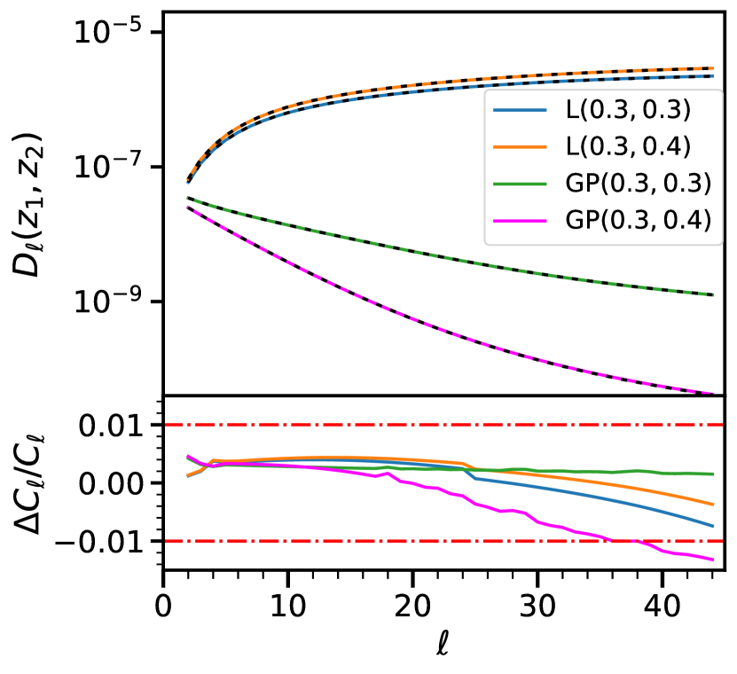
(a)

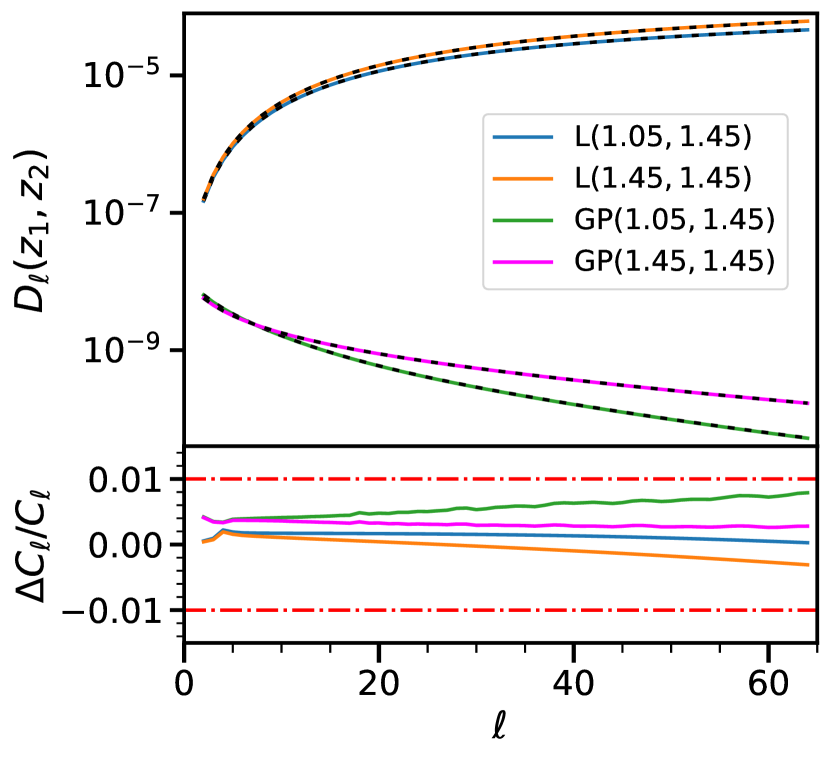
(b)

Figure 10: The multipole-scaled angular power spectrum $D_{\ell}\equiv\ell(\ell+1)/(2\pi)C_{\ell}$ and the relative difference $(C_{\ell}^{\rm SFB}-C_{\ell}^{\rm class})/C_{\ell}^{\rm class}$ between our SFB-transformed results and the CLASS outputs. In the upper panels, the solid lines represent the CLASS output, while the dashed black lines show the corresponding angular power spectrum transformed from our SFB PS results. In both panels, the different colors indicate the different GR effects and different redshifts considered. In the legend, "L" indicates the lensing-lensing term, while "GP" indicates the GP-GP term that includes Shapiro, ISW, and NIP effects. The two numerical values inside the bracket indicate the two redshifts where the angular power spectrum is computed. The left and right subplots consider the lower ($z=0.2-0.5$) and the higher ($z=1.0-1.5$) redshift ranges respectively.

Our validation of GR effects in SFB will rely on the SFB-to-TSH mapping in eq. A.7. We can transform our SFB results into TSH using eq. A.7 and then compare with the TSH results directly calculated from CLASS. The number count angular power spectrum in CLASS has been implemented with both brute-force integration [12] and FFTlog method [13], with both methods agreeing at $0.1\%$ for the angular PS of the total relativistic number count. Our numerical implementation of the SFB power spectrum is completely independent from CLASS, and the angular power spectrum is only obtained as the last step from our SFB calculation using the mapping such that we can compare with the existing public code on GR effects.

In the summation of eq. A.7, we consider $n_{1}$ and $n_{2}$ with $k_{n\ell}\leq 0.25h/{\rm Mpc}$ to truncate the smaller radial modes. We consider the TSH obtained from both auto-correlation at one redshift and cross-correlation between two redshifts. The bias parameters are set as the same ones chosen in section 5. We show our validation results in figure 10 for the lensing-lensing and GP-GP terms at different redshifts.

In general, our SFB-transformed TSH results for the two individual GR terms agree within the percent level of the corresponding CLASS outputs at both low (figure 10(a)) and high redshifts (figure 10(b)) for multipoles $2\leq\ell\lessapprox 40$. This demonstrates the accuracy of our implementation of the lensing and GP terms in the SFB PS. Since the calculation of the Newtonian RSD and Doppler terms have already been validated through mocks in Refs. [35, 23], and the GP term contains the NIP, Shapiro, and ISW effects, we have therefore validated the SFB calculation for all terms present in the relativistic number count.

Our SFB-transformed TSH begins to diverge from the CLASS outputs, gradually surpassing the percentage levels for higher multipoles $\ell\gtrapprox 60$ as seen in figure 10. This deviation is expected, since one has to include more radial SFB modes evaluated at higher $k_{n\ell}$ than our truncation limit $0.25h/{\rm Mpc}$ to obtain more accurate TSH for higher angular multipoles. Since CLASS uses the full linear transfer function from solving the Boltzmann equations, while our SFB computation relies on the $\Lambda$CDM approximations given in eqs. 4.10, 4.11, 4.12 and 4.13, in addition to the errors introduced by the $k_{n\ell}$ truncation in the TSH-SFB mapping, we expect pushing our validation below the percent-level agreement to be difficult. However, the total GR effect only produces percent-level correction (below $10\%$ as seen in figure 6) at redshift $z\leq 2$, we consider achieving percent-level agreement on the GR corrections sufficient for validating the accuracy of our implementation.

Appendix D Lensing Approximation

D.1 Limber Approximation on LOS Integral

In this section, we aim to gain some intuition for the lensing term in the SFB power spectrum by employing the Limber approximation on the LOS integral in eq. 2.4. At the first-order, the Limber approximation is [123]:

$$j_{\ell}(kr) \simeq\sqrt{\frac{\pi}{2rk}}\frac{1}{k}\delta^{D}(r-\frac{\ell+\frac{1}{2}}{k})\,.$$ (D.1)

The above approximation applies when all other functions are slowly-varying compared to the frequency of the spherical Bessel functions, and the integration should be over a wide interval.

Applying the Limber approximation to the lensing angular kernel in eq. 4.6, we have

$$\Delta_{\ell}(x,q)^{\rm Lensing}\approx\ell(\ell+1)\frac{2-5s(x)}{2}\int_{r=0}^{\infty}\mathbb{I}_{[r\leq x]}\frac{x-r}{xr}(\Phi(r,q)+\Psi(r,q))\sqrt{\frac{\pi}{2rq}}\frac{1}{q}\delta^{D}(r-\frac{\ell+\frac{1}{2}}{q})$$

$$=\sqrt{\frac{\pi}{2(\ell+\frac{1}{2})}}\ell(\ell+1)\frac{2-5s(x)}{2}\left(\frac{1}{\ell+\frac{1}{2}}-\frac{1}{qx}\right)\left(\Phi(\frac{\ell+\frac{1}{2}}{q},q)+\Psi(\frac{\ell+\frac{1}{2}}{q},q)\right)\mathbb{I}_{[(\ell+\frac{1}{2})/q\leq x]}\,,$$ (D.2)

where $\mathbb{I}_{[...]}$ is the indicator function. We see that the LOS integral is mostly determined by the gravitational potentials at an effective position $x_{\rm lens}=(\ell+\frac{1}{2})/q$ for each combination of the Fourier mode $q$ and angular mode $\ell$. The source galaxy at $x$ is effectively lensed by the structure at $x_{\rm lens}$ for a given SFB mode. If the Fourier scale $q$ is fixed, then increasing the angular scale will shift the effective lens plane to a higher redshift.

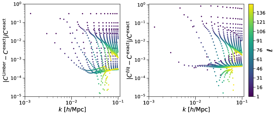
Figure 11: The accuracy of two approximations for the lensing-lensing term in the diagonal part of the SFB power spectrum for the redshift range from $z=1.0$ to $1.5$. The left panel shows the accuracy of eq. D.2, where the Limber approximation is applied to the LOS integral in the lensing angular kernel. The right panel shows the accuracy of eq. D.3, where the explicit dependence of the lensing angular kernel on $\ell$ and $q$ are eliminated. The accuracy of both methods primarily depend on the angular multipoles $\ell$, and they agree with the exact calculation at the percent level for $\ell\gtrapprox 50$.

As shown in the left panel of figure 11, the limber approximation deviates from the exact results of the lensing-lensing term by tens of percent at the largest angular scales across the Fourier modes $k$, but it becomes accurate within the percent level for higher angular multipoles. This potentially suggests that one can use the Limber approximation to further speed up the evaluation of the lensing effect in the SFB power spectrum at smaller angular scales by avoiding the LOS integral. However, the exact applicability of the approximation will depend on the accuracy required by the specific science goal, and it should be examined for each survey. We note that the Limber approximation on the LOS integral also applies to other integrated effects including the Shapiro and ISW effects.

D.2 $\ell/q$-Approximation

Here we will examine the accuracy of the following approximation for the lensing angular kernel:

$$\Delta_{\ell}(x,q)^{\rm Lensing} \approx\frac{3\Omega_{\rm m,0}H_{0}^{2}}{2}\left(2-5s(x)\right)\int_{0}^{x}dr\,r\frac{r-x}{x}(1+z(r))D(r)j_{\ell}(qr)\,.$$ (D.3)

The above approximation for the lensing magnification is often used for calculating the angular power spectrum in literature [124, 125, 126, 53], and it has been used for computing the SFB PS in Ref. [32].

To see how eq. D.3 can be obtained, we substitute the density and gravitational potential transfer functions eqs. 4.10 and 4.12 under the $\Lambda$CDM model into the exact expression of eq. 4.6:

$$\Delta_{\ell}(x,q)^{\rm Lensing} =\frac{3}{2}\frac{\ell(\ell+1)}{q^{2}}\left(2-5s(x)\right)\int_{0}^{x}dr\,\frac{r-x}{xr}\mathcal{H}(r)^{2}\Omega_{\rm m}(r)D(r)j_{\ell}(qr)$$

$$=\frac{3\Omega_{\rm m,0}H_{0}^{2}}{2}\left(2-5s(x)\right)\int_{0}^{x}dr\,\frac{\ell(\ell+1)}{q^{2}}\frac{r-x}{xr}(1+z(r))D(r)j_{\ell}(qr)\,.$$ (D.4)

Motivated by the Limber approximation, we can approximate the $\ell(\ell+1)/q^{2}$ factor in eq. D.4 as $r^{2}$ to obtain eq. D.3. We refer to this scheme as the "$\ell/q$-approximation", since the explicit dependence of the lensing angular kernel on $\ell$ and $q$ has been dropped.

Similar to the Limber approximation applied to the LOS integral, the $\ell/q$-approximation is inaccurate at the largest angular scales and becomes more accurate for the lensing SFB PS when one considers higher $\ell$ values, as shown in the right panel of figure 11. Despite the accuracy of this approximation, it does not achieve significant computational speedup for evaluating the SFB power spectrum, since the LOS integral remains in the angular kernel, and the dimension of the integral under the approximation is the same as the exact expression. We therefore recommend using the exact angular kernel eq. 4.6 when computing the SFB PS.

Appendix E Infrared Divergence in Monopole

We have so far computed the SFB power spectrum for angular multipoles $\ell\geq 1$. We now discuss the computation of the SFB monopole and observe its divergence for angular kernels of the form:

$$\Delta_{\ell}^{\rm Div}(x,q)=\frac{1}{q^{2}}j_{\ell}(qx)A(x)\,,$$ (E.1)

where $A(x)$ absorbs both the radial window and redshift evolution. For the DRSD and Doppler terms, their monopole is convergent. The lensing term does not contribute to the monopole since its angular kernel is proportional to $\ell(\ell+1)$ as seen in eq. 4.6. In comparison, the angular kernels for the NIP, Shapiro, ISW, and PNG terms have the same $1/q^{2}$ behavior as in eq. E.1 due to their proportionality to the gravitational potential, and the correlation among these terms will diverge for the SFB monopole in both the continuous and discrete SFB basis.

E.1 Divergence in Discrete SFB

For the discrete SFB power spectrum computed in eq. 4.1, we have

$$C_{\ell nn^{\prime}}^{\rm Div} =\frac{2}{\pi}\int_{0}^{\infty}dq\,\frac{1}{q^{2}}\left[\int_{x_{\rm min}}^{x_{\rm max}}dx\,x^{2}g_{n\ell}(x)j_{\ell}(qx)A(x)\right]$$

$$\qquad\left[\int_{x_{\rm min}}^{x_{\rm max}}dx^{\prime}\,x^{\prime 2}g_{n^{\prime}\ell}(x^{\prime})j_{\ell}(qx^{\prime})A(x^{\prime})\right]P_{\rm m,0}(q)\,.$$ (E.2)

In general, the spherical Bessel function has the asymptotic behavior $j_{\ell}(y)\sim O(y^{\ell})$ for $y\to 0$. We see that for higher multipoles $\ell\geq 1$, the integrand behaves as $q^{2\ell-2}P_{\rm m,0}(q)$, which will lead to convergence in the above integral. Therefore, there is no divergence for any GR terms in SFB multipoles $\ell\geq 1$.

For the monopole $\ell=0$, the integrand now scales as $q^{-2}P_{\rm m,0}(q)\sim q^{-2+n_{s}}$, where $n_{s}$ is the scalar index for the primordial perturbation spectrum. Since the measurement of CMB anisotropies has strongly constrained the scalar index to be $n_{s}<1$ [43], the scaling behavior of $q^{-2+n_{s}}$ will cause divergence in eq. E.2, that is $C_{0nn^{\prime}}$ diverge for all $n$ and $n^{\prime}$ regardless of the boundary conditions. Therefore, the correlation among the NIP, Shapiro, ISW, and PNG terms will be divergent for the discrete SFB monopole at all Fourier modes.

E.2 Divergence in Continuous SFB

When $A(x)$ is regulated by some radial selection function with finite coverage from $x_{\rm min}$ to $x_{\rm max}$, the continuous SFB monopole from eq. B.8 becomes:

$$C_{0}^{\rm R,Div}(k,k^{\prime}) =\frac{2}{\pi}\int_{0}^{\infty}dq\,\frac{1}{q^{2}}\left[\int_{x_{\rm min}}^{x_{\rm max}}dx\,\,x^{2}j_{0}(kx)j_{0}(qx)A(x)\right]$$

$$\qquad\left[\int_{x_{\rm min}}^{x_{\rm max}}dx^{\prime}\,\,x^{\prime 2}j_{0}(k^{\prime}x^{\prime})j_{0}(qx^{\prime})A(x^{\prime})\right]P_{\rm m,0}(q)$$ (E.3)

Similar to the above arguments in the discretized case, all $C_{0}(k,k^{\prime})$ diverges regardless of the Fourier modes, since the integral $\int_{x}x^{2}j_{0}(kx)j_{0}(qx)A(x)$ will always be finite when we integrate over some finite range, which does not help to tame the divergence caused by $q^{-2}$.

We now consider an idealized case of the infinite universe. Assuming that $A(x)=A$ is uniform across the entire configuration space without the presence of any window, we see that for all angular multipoles including the monopole, the CSFB PS of the divergent terms becomes

$$C_{\ell}^{\rm Div}(k,k^{\prime}) =\frac{2A^{2}}{\pi}\int_{0}^{\infty}dq\,\frac{1}{q^{2}}\left[\int_{0}^{\infty}dx\,x^{2}j_{\ell}(kx)j_{\ell}(qx)\right]\left[\int_{0}^{\infty}dx^{\prime}\,x^{\prime 2}j_{\ell}(k^{\prime}x^{\prime})j_{\ell}(qx^{\prime})\right]P_{\rm m,0}(q)$$

$$=\frac{2A^{2}}{\pi}\int_{0}^{\infty}dq\,\frac{1}{q^{2}}\frac{\pi}{2kq}\delta^{\rm D}(k-q)\frac{\pi}{2k^{\prime}q}\delta^{\rm D}(k^{\prime}-q)P_{\rm m,0}(q)$$

$$=\frac{\pi A^{2}}{4}\frac{1}{k^{6}}P_{\rm m,0}(k)\delta^{\rm D}(k-k^{\prime}),$$ (E.4)

using the orthogonality of spherical Bessel functions in eq. G.3. Therefore, in the case where one ignores the radial window function, the $k^{-4}$ scaling behavior for the divergent terms is exactly recovered in the CSFB PS, and we can see that the CSFB monopole converges at all Fourier modes except $k=0$.

The behavior of eq. E.4 in the infinite universe also explains the divergence of the CSFB monopole at all Fourier modes in the presence of radial window function in eq. E.3. In the infinite case, only $C_{0}(0,0)$ diverges, but the $k=0$ mode in the infinite case is mixed to all other $k$ modes after the window convolution, which causes the divergence of the CSFB monopole $C_{0}^{\rm R}(k,k^{\prime})$ with radial window at all Fourier modes.

E.3 Practical and Theoretical Considerations

Fortunately, the divergence of the SFB monopole in individual GR terms is practically irrelevant for galaxy surveys due to the presence of integral constraint [41] (also known as local average effects  [35, 127]), i.e. the true average galaxy density is unknown but estimated from the survey itself. Without the presence of any angular mask (that is a window function with only radial selection), the measured SFB monopole at all Fourier modes is forced to be zero due to the radial integral constraint [35, 108], and the cosmological SFB monopole becomes un-observable. Therefore, the divergence of the SFB monopole for the GP and PNG terms is of no concern when analyzing galaxy surveys.

However, the divergence of the SFB monopole is still of theoretical interest. Even though the individual NIP, ISW, and Shapiro effects are divergent in the SFB monopole, the divergence in the GP term will cancel out once the observer’s potential, which we have ignored in this work, is consistently included. Ref. [128] has argued for the general cancellation of the infrared-divergent terms under a gauge-invariant, order-consistent GR calculation, while Refs. [129], [130], and [17] have explicitly shown the cancellation of the divergent linear-order GR terms for the Fourier-space galaxy power spectrum, the angular monopole, and the configuration-space correlation function respectively. We will explicitly show the divergence cancellation and calculate the SFB monopole under the linear-order GR effects including the observer’s terms in a forthcoming work.

In contrast to the GR terms where infrared divergence will cancel out, the PNG-PNG term (proportional to $f_{\rm NL}^{2}$) is genuinely divergent in the SFB monopole. Though initially formulated in the Newtonian theory, the scale-dependent bias due to the local PNG is consistent with the relativistic context as we have reviewed in section 2.2. Such divergence is in fact a signature of the local PNG effect, since it is sensitive to the super-sample value of the gravitational potential due to the coupling of the large and small scales during the structure formation. Despite the apparent degeneracy between the GP and PNG terms in the $\ell$-$k$ space as shown in figure 8, the divergence in monopole differentiates the physical mechanisms behind the two terms.

Appendix F Iso-qr Integration

In this appendix, we explain our numerical calculation of integrals of the form

$$\int_{r_{\mathrm{min}}}^{r_{\mathrm{max}}}f(r,q)\,j_{\ell}(qr)\,,$$ (F.1)

where $f(r,q)$ is cheap to calculate, but $j_{\ell}(qr)$ is expensive. This is the same algorithm, but a more detailed description of what was done in Sec. IV of Ref. [35]. We refer to this algorithm as the Iso-qr integration. We will first motivate why other approaches are slow or why we have not considered them, yet, then we derive the requirements for our approach to work. Finally, we go beyond our initial implementation [35] and add a restarted-integration that significantly reduces the number of sampling points needed when the integration interval is large.

Fundamentally, the approach detailed here is a brute-force trapezoidal integration. Crucial is our assumption that in eq. F.1 the function $f(r,q)$ is fast to evaluate, while $j_{\ell}(qr)$ is expensive. This allows for $f(r,q)$ to change frequently (hence the need for efficient evaluation of eq. F.1), while the spherical Bessel $j_{\ell}(qr)$ will be quite static and can be precomputed. However, the speed of our brute-force integration comes from an informed choice of the integration nodes, which allows the cache of precomputed $j_{\ell}(qr)$ to be very small.

F.1 Motivation

Before we go into detail of our integration method, we review other (often similar) approaches.

Precompute:

A simple speedup of the integration can be achieved by precomputing the spherical Bessels. However, this means creating an array of $N=N_{d}\,N_{\ell}\,N_{q}\,N_{r}\simeq 4\cdot 200\cdot 1000\cdot 1000$ floating point numbers, or about 6 GB of storage, where $N_{d}$ is the number of derivatives needed on the spherical Bessel functions, $N_{\ell}$ is the number of $\ell$, $N_{q}$ is the number of sampling points in $q$ that are desired, and $N_{r}$ is the number of sampling points in $r$ that are needed for reasonably accurate evaluation of the integral. For a large redshift range these memory requirements can easily be a factor of a few larger. It takes both time and memory to precompute all of this, and leaves little memor0y for other tasks such as the window convolution.

Spline:

An alternative would be to create splines of the spherical Bessels. The storage here would be reduced to a 2D array, since the argument can be sampled linearly from $(qr)_{\mathrm{min}}=q_{\mathrm{min}}r_{\mathrm{min}}$ to $(qr)_{\mathrm{max}}=q_{\mathrm{max}}r_{\mathrm{max}}$. However, splines generally require many if-statements with unpredictable branching behavior especially during the hunting phase on each call. This means spending several tens of CPU cycles on each grid point.

FFTLog:

Equation F.1 is almost in a form suitable for the FFTLog algorithm [131]. However, FFTLog has two problems: first, it is not a robust algorithm, and requires apodization and zero-padding when the integration is over a finite interval. Second, FFTLog requires the function $f(r,q)$ to be separable so that the $q$-dependence can be taken outside the integral. Therefore, should $f(r,q)$ be separable at all, it would require some additional work to expand $f(r,q$) in separable terms. In any case, the first problem calls for a more robust integration scheme that can serve as reference for a possible FFTLog implementation in the future.

F.2 Iso-$qr$ lines

As mentioned in section F.1, the expensive function $j_{\ell}(qr)$ only depends on the product $qr$, not on $q$ and $r$ individually. Therefore, only a 2D array with dimensions in $\ell$ and $x=qr$ need be precomputed on some grid points $(x_{m},\ell_{k})$.

Neighboring points:

We can find discretizations of $q$ and $r$ such that all $qr$ fall on a few iso-$qr$ lines, as follows. Let $q_{i}$ and $r_{j}$ be discrete points. Then, we desire that there are neighboring grid points that fall on the same iso-$qr$ line. For example, if we go up one grid point from $q_{i}$ to $q_{i+1}$, then we will need to go down in $r$ from $r_{i}$ to $r_{i-1}$. For the product to be the same, we require that

$$x_{m} =q_{i}\,r_{j}=q_{i+1}\,r_{j-1}\,.$$ (F.2)

Equation F.2 implies that

$$d\ln q=\ln\frac{q_{i+1}}{q_{i}}=\ln\frac{r_{j}}{r_{j-1}}=d\ln r\,.$$ (F.3)

That is, for points on an iso-$qr$ line, the logarithmic spacings of $q$ and $r$ must have the same step size, or $d\ln q=d\ln r$.

Many points:

Since we also wish to reuse the same grid points $(q_{i},r_{j})$ for other iso-$qr$ lines, it means that the spacing for both $q$ and $r$ needs to be logarithmic throughout the entire integration plane. The mapping from $(i,j)$ to the index $m$ in eq. F.2 is simply $m=i+j-1$.

For the integration in log-space, we choose a simple mid-point trapezoidal rule, which will be simplest when the number of subdivisions is an integer. If $N_{r}$ is the number of desired subdivisions in $r$, then

$$R=d\ln r=\frac{\ln r_{\mathrm{max}}-\ln r_{\mathrm{min}}}{N_{r}}\,,$$ (F.4)

and the corresponding grid points are

$$r_{j}=r_{\mathrm{min}}\,e^{(j-\frac{1}{2})R}\,,$$ (F.5)

where $j=1,2,\ldots,N_{r}$. The factor $e^{\frac{1}{2}R}$ ensures that the grid points fall in the middle of each interval.

F.3 Striding

Figure 12: The $qr$ grid in log-space. Solid lines show the $qr=\mathrm{const}$ lines, dashed lines show possible integration paths, here with skipping some of the $q$ points. The axis labels refer to $i$ and $j$, respectively.

Stride:

It is our desire to use as few grid points as possible. Indeed, we can skip some of the $q_{i}$. If we request $\tilde{N}_{q}$ grid points in $q$, then our requirement of using the same logarithmic spacing as in $r$ means that we need to skip $\tilde{s}_{q}-1$ grid points, we call $\tilde{s}_{q}$ the stride. Its value is given by

$$\tilde{s}_{q} =\frac{\ln q_{\mathrm{max}}-\ln q_{\mathrm{min}}}{\tilde{N}_{q}\,d\ln r}\,.$$ (F.6)

To gain some intuition for this equation, imagine $\tilde{N}_{q}=1$. Then, we should skip all but one $q$ grid point, so $\tilde{s}_{q}$ is very large. If, on the other hand, $\tilde{N}_{q}$ happens to be the number of logarithmic subdivisions of size $d\ln r$, then we shouldn’t skip any, and our stride is $\tilde{s}_{q}=1$.

Integer stride:

Of course, the actual stride $s_{q}$ must be an integer, and we round $\tilde{s}_{q}$ down to obtain it. That also means that the actual number $N_{q}$ of grid points cannot be equal to the desired number $\tilde{N}_{q}$ of grid points, or $N_{q}\neq\tilde{N}_{q}$ in general. Similarly, only one of $q_{\rm min}$ and $q_{\rm max}$ can be exactly included as a grid point. In case the exact interval is needed, one (expensive) extra step will need to be included in the integration.

Figure 12 illustrates the grid with $s_{q}=2$. A stride $s_{r}$ in $r$ can also differ from unity, and we allow for strides in both axes below. Important for the implementation is how to map $(i,j)$ to $m$. We use

$$m =1+(i-1)\,s_{q}+(j-1)\,s_{r}\,,$$ (F.7)

for $i=1,\ldots,N_{q}$, $j=1,\ldots,N_{r}$, and $m=1,\ldots,N_{j_{l}}$, where $N_{j_{l}}$ is the number of spherical Bessels that need to be stored.

F.4 Sampling needs

To get a reasonably accurate estimation of eq. F.1, the numerically calculated integrand needs to sufficiently sample the oscillations of the spherical Bessel functions. We only use the spherical Bessel in this step, because we assume that the function $f(r,q)$ is smooth and varies on the same scales or slower.

Sampling spherical Bessels:

Since the spherical Bessels asymptote to $j_{\ell}(x)\to\sin(x+\phi_{\ell})/x$ as $x\to\infty$, and the frequency of oscillations is only lower towards $x\to 0$, we desire a maximum $\Delta x$ of

$$\Delta x\leq\frac{2\pi}{n_{\mathrm{samp}}}\,,$$ (F.8)

where $n_{\mathrm{samp}}$ is the number of sampling points in one oscillation. Due to the logarithmic spacing, the largest $\Delta x_{m}$ will be given at $x_{\mathrm{max}}=q_{\mathrm{max}}r_{\mathrm{max}}$, and this informs the total number of sampling points $N_{r}$ and $N_{q}$.

F.5 Interval Integration

The logarithmic sampling required by our $qr$-integration method can lead to a very fine sampling near the lower integration bound, e.g., if $r_{\min}\sim 0$, as occurs for the integrated GR terms. In this case, we can divide the integration range into smaller intervals, and apply the method on each interval individually. The subdividing can be done recursively, until the lower bound is smaller than the largest step. In practice, this buys about a factor two in speedup.

Crucial is that the $q$ array remains the same across each interval. That is, we first choose a $q$ array, and then we will choose the individual $r$ arrays in each interval. If the logarithmic spacing in $q$ is $Q=\differential\ln q$, and the spacing in $r$ is $R_{n}=\differential\ln r_{n}$ at the $n^{\rm th}$ interval, our integration technique requires that

$$\frac{R_{n}}{s_{r}^{n}} =\frac{Q}{s^{n}_{q}}\,,$$ (F.9)

where $s^{n}_{r}$ and $s^{n}_{q}$ are positive integers. $s^{n}_{q}$ is the stride in $q$ relative to a fictitious $\differential\ln r=Q/s^{n}_{q}$, and $s^{n}_{r}$ is the stride in $r$ relative to that same fictitious $\differential\ln r$.

If $N_{r}^{n}$ is the number of integration nodes in interval $n$, then the width of the interval in log space is $N^{n}_{r}\,R_{n}=N_{r}^{n}\,s_{n}\,Q$, and we defined $s_{n}\equiv s^{n}_{r}/s^{n}_{q}$. All intervals together must add to approximately the full interval,

$$\ln r_{\max}-\ln r_{\min}\geq Q\sum_{n}N^{n}_{r}\,s_{n}\,,$$ (F.10)

where the inequality will need to be overcome by an extra integration step discussed below. The maximum $\ln r$ in each interval is

$$\ln b_{n} =\ln r_{\max}-Q\sum_{i=n+1}^{n_{\max}}N_{r}^{i}\,s_{i}\,,$$ (F.11)

so that the $n^{\mathrm{th}}$ interval ranges from $b_{n-1}$ to $b_{n}$, and intervals are labeled by counting from the bottom, i.e., the interval $n=1$ has lower bound $\simeq r_{\min}$, and the interval $n_{\max}$ as upper bound $r_{\max}$.

The precision of the integration is controled by requiring that the maximum linear integration step is below some $\Delta r_{\max}$ for every interval,

$$\Delta r_{\max}\geq b_{n}R_{n}=\frac{r_{\max}\,s_{n}\,Q}{\exp(Q\sum_{n+1}^{n_{\max}}N^{n}_{r}\,s_{n})}\,.$$ (F.12)

Solving for $s_{n}$ we obtain,

$$s_{n} \leq\frac{\Delta r_{\max}}{Q\,r_{\max}}\,\exp(Q\sum_{n+1}^{n_{\max}}N^{n}_{r}\,s_{n})\,,$$ (F.13)

which is a series of equations for each $n$. When $n=n_{\max}$ this gives a maximum value for $s_{n_{\max}}\leq\frac{\Delta r_{\max}}{Q\,r_{\max}}$, and using this value will maximize the step size in the upper-most interval.

$s_{n_{\max}}$ in turn can be used to calculate the minimum $N_{r}^{n_{\max}}$, provided that $s_{n_{\max}-1}$ is given, or, more generally,

$$N^{n}_{r} \geq\frac{1}{s_{n}\,Q}\ln\frac{s_{n-1}}{s_{n}}\,,$$ (F.14)

which requires all the $s_{n}$ to be given. Using eq. F.10 we get the constraint

$$\ln\frac{r_{\max}}{r_{\min}} \geq\sum_{n}\ln\frac{s_{n-1}}{s_{n}}\,,$$ (F.15)

which will need to be checked so as not to overshoot $r_{\min}.$

The last step from slightly above $r_{\min}$ to $r_{\min}$ can be done with a single step of arbitrary width such that the full integration interval from $r_{\min}$ to $r_{\max}$ is included.

The goal, now is to find integer strides $s_{q}^{n}\geq 1$ and $s_{r}^{n}\geq 1$ that satisfy these constraints with $s_{n}=s_{r}^{n}/s_{q}^{n}$, and that minimize the size of the $qr$-qr and $j_{l}$-cache. For a given $\ell$, the number of grid points is given by

$$N_{qr}^{\mathrm{total}} =N_{q}\sum_{n}N^{n}_{r}\,,$$ (F.16)

and the number of spherical Bessel evaluations is [cf. eq. F.7]

$$N_{j_{l}}^{\mathrm{total}} =N_{d}\sum_{n}\left[1+(N_{q}-1)s^{n}_{q}+(N_{r}^{n}-1)s^{n}_{r}\right],$$ (F.17)

where $N_{d}$ is the number of derivatives of the spherical Bessels that are needed. We then minimize some combination $F(s^{n}_{q},s^{n}_{r})=N_{qr}^{\mathrm{total}}+\beta N_{j_{l}}^{\mathrm{total}}$ for some $\beta$. The choice $\beta=1$ is natural as it will minimize the number of memory locations that need to be accessed. We have now generalized the Iso-qr integration to multiple subintervals of $r$, while ensuring the $q$ array to remain the same across the entire interval.

Appendix G Useful Identities

Orthogonality of spherical harmonics:

$$\int d^{2}\hat{\mathbf{k}}~{}Y_{\ell m}(\hat{\mathbf{k}})Y^{*}_{\ell^{\prime}m^{\prime}}(\hat{\mathbf{k}})=\delta_{\ell\ell^{\prime}}\delta_{mm^{\prime}}\,.$$ (G.1)

Rayleigh expansion of a plane wave:

$$e^{i\mathbf{k}\cdot\mathbf{x}}=(4\pi)\sum_{\ell m}i^{\ell}j_{\ell}(kx)Y_{\ell m}(\hat{\mathbf{x}})Y_{\ell m}^{*}(\hat{\mathbf{k}})\,.$$ (G.2)

Orthogonality of spherical Bessel functions:

$$\int_{r}r^{2}j_{\ell}(kr)j_{\ell}(k^{\prime}r)=\frac{\pi}{2kk^{\prime}}\delta^{{\rm D}}(k-k^{\prime}).$$ (G.3)

References

- [1] DESI collaboration, The DESI Experiment Part I: Science,Targeting, and Survey Design, 1611.00036.
- [2] L. Amendola et al., Cosmology and fundamental physics with the Euclid satellite, Living Rev. Rel. 21 (2018) 2 [1606.00180].
- [3] Ž. Ivezić, S. M. Kahn, J. A. Tyson, B. Abel, E. Acosta, R. Allsman et al., LSST: From Science Drivers to Reference Design and Anticipated Data Products, ApJ 873 (2019) 111 [0805.2366].
- [4] O. Doré, J. Bock, M. Ashby, P. Capak, A. Cooray, R. de Putter et al., Cosmology with the SPHEREX All-Sky Spectral Survey, arXiv e-prints (2014) arXiv:1412.4872 [1412.4872].
- [5] T. Eifler et al., Cosmology with the Roman Space Telescope: synergies with the Rubin Observatory Legacy Survey of Space and Time, Mon. Not. Roy. Astron. Soc. 507 (2021) 1514 [2004.04702].
- [6] M. Noorikuhani and R. Scoccimarro, Wide-angle and relativistic effects in Fourier-space clustering statistics, Phys. Rev. D 107 (2023) 083528 [2207.12383].
- [7] M. Foglieni, M. Pantiri, E. Di Dio and E. Castorina, Large Scale Limit of the Observed Galaxy Power Spectrum, Phys. Rev. Lett. 131 (2023) 111201 [2303.03142].
- [8] D. Alonso, P. Bull, P. G. Ferreira, R. Maartens and M. G. Santos, Ultra-large-scale Cosmology in Next-generation Experiments with Single Tracers, ApJ 814 (2015) 145 [1505.07596].
- [9] D. Alonso, P. Bull, P. G. Ferreira, R. Maartens and M. G. Santos, Ultra-large-scale Cosmology in Next-generation Experiments with Single Tracers, ApJ 814 (2015) 145 [1505.07596].
- [10] A. Challinor and A. Lewis, Linear power spectrum of observed source number counts, Phys. Rev. D 84 (2011) 043516 [1105.5292].
- [11] C. Bonvin and R. Durrer, What galaxy surveys really measure, Phys. Rev. D 84 (2011) 063505 [1105.5280].
- [12] E. Di Dio, F. Montanari, J. Lesgourgues and R. Durrer, The CLASSgal code for relativistic cosmological large scale structure, JCAP 2013 (2013) 044 [1307.1459].
- [13] N. Schöneberg, M. Simonović, J. Lesgourgues and M. Zaldarriaga, Beyond the traditional line-of-sight approach of cosmological angular statistics, JCAP 2018 (2018) 047 [1807.09540].
- [14] A. Lewis, A. Challinor and A. Lasenby, Efficient computation of CMB anisotropies in closed FRW models, ApJ 538 (2000) 473 [astro-ph/9911177].
- [15] D. Blas, J. Lesgourgues and T. Tram, The Cosmic Linear Anisotropy Solving System (CLASS). Part II: Approximation schemes, JCAP 2011 (2011) 034 [1104.2933].
- [16] V. Tansella, C. Bonvin, R. Durrer, B. Ghosh and E. Sellentin, The full-sky relativistic correlation function and power spectrum of galaxy number counts. Part I: theoretical aspects, JCAP 2018 (2018) 019 [1708.00492].
- [17] E. Castorina and E. Di Dio, The observed galaxy power spectrum in General Relativity, JCAP 2022 (2022) 061 [2106.08857].
- [18] V. Tansella, G. Jelic-Cizmek, C. Bonvin and R. Durrer, COFFE: a code for the full-sky relativistic galaxy correlation function, JCAP 2018 (2018) 032 [1806.11090].
- [19] J. Yoo and U. Seljak, Wide-angle effects in future galaxy surveys, MNRAS 447 (2015) 1789 [1308.1093].
- [20] P. Reimberg, F. Bernardeau and C. Pitrou, Redshift-space distortions with wide angular separations, JCAP 2016 (2016) 048 [1506.06596].
- [21] E. Castorina and M. White, Beyond the plane-parallel approximation for redshift surveys, MNRAS 476 (2018) 4403 [1709.09730].
- [22] J. N. Benabou, I. Sands, H. S. Grasshorn Gebhardt, C. Heinrich and O. Doré, Wide-Angle Effects in the Power Spectrum Multipoles in Next-Generation Redshift Surveys, arXiv e-prints (2024) arXiv:2404.04811 [2404.04811].
- [23] R. Y. Wen, H. S. Grasshorn Gebhardt, C. Heinrich and O. Doré, Exact Modeling of Power Spectrum Multipole through Spherical Fourier-Bessel Basis, arXiv e-prints (2024) arXiv:2404.04812 [2404.04812].
- [24] B. Leistedt, A. Rassat, A. Réfrégier and J. L. Starck, 3DEX: a code for fast spherical Fourier-Bessel decomposition of 3D surveys, A&A 540 (2012) A60 [1111.3591].
- [25] J. Yoo and V. Desjacques, All-sky analysis of the general relativistic galaxy power spectrum, Phys. Rev. D 88 (2013) 023502 [1301.4501].
- [26] G. Pratten and D. Munshi, Effects of linear redshift space distortions and perturbation theory on BAOs: a 3D spherical analysis, MNRAS 436 (2013) 3792 [1301.3673].
- [27] A. Nicola, A. Refregier, A. Amara and A. Paranjape, Three-dimensional spherical analyses of cosmological spectroscopic surveys, Phys. Rev. D 90 (2014) 063515 [1405.3660].
- [28] F. Lanusse, A. Rassat and J. L. Starck, 3D galaxy clustering with future wide-field surveys: Advantages of a spherical Fourier-Bessel analysis, A&A 578 (2015) A10 [1406.5989].
- [29] A. Liu, Y. Zhang and A. R. Parsons, Spherical Harmonic Analyses of Intensity Mapping Power Spectra, ApJ 833 (2016) 242 [1609.04401].
- [30] L. Samushia, Proper Fourier decomposition formalism for cosmological fields in spherical shells, arXiv e-prints (2019) arXiv:1906.05866 [1906.05866].
- [31] M. S. Wang, S. Avila, D. Bianchi, R. Crittenden and W. J. Percival, Hybrid-basis inference for large-scale galaxy clustering: combining spherical and Cartesian Fourier analyses, JCAP 2020 (2020) 022 [2007.14962].
- [32] Y. Zhang, A. R. Pullen and A. S. Maniyar, Joint analyses of 2D CMB lensing and 3D galaxy clustering in the spherical Fourier-Bessel basis, Phys. Rev. D 104 (2021) 103523 [2110.00872].
- [33] H. S. Grasshorn Gebhardt and O. Doré, Fabulous code for spherical Fourier-Bessel decomposition, Phys. Rev. D 104 (2021) 123548 [2102.10079].
- [34] B. Khek, H. S. Grasshorn Gebhardt and O. Doré, Fast Theoretical Predictions for Spherical Fourier Analysis of Large-Scale Structures, arXiv e-prints (2022) arXiv:2212.05760 [2212.05760].
- [35] H. Grasshorn Gebhardt and O. Doré, Validation of Spherical Fourier-Bessel power spectrum analysis with lognormal simulations and eBOSS DR16 LRG EZmocks, arXiv e-prints (2023) arXiv:2310.17677 [2310.17677].
- [36] J. N. Benabou, A. Testa, C. Heinrich, H. S. Grasshorn Gebhardt and O. Doré, The Galaxy Bispectrum in the Spherical Fourier-Bessel Basis, arXiv e-prints (2023) arXiv:2312.15992 [2312.15992].
- [37] F. Semenzato, D. Bertacca and A. Raccanelli, The full-sky Spherical Fourier-Bessel power spectrum in general relativity, arXiv e-prints (2024) arXiv:2406.09545 [2406.09545].
- [38] A. Hall, C. Bonvin and A. Challinor, Testing general relativity with 21-cm intensity mapping, Phys. Rev. D 87 (2013) 064026 [1212.0728].
- [39] Square Kilometre Array Cosmology Science Working Group, D. J. Bacon, R. A. Battye, P. Bull, S. Camera, P. G. Ferreira et al., Cosmology with Phase 1 of the Square Kilometre Array Red Book 2018: Technical specifications and performance forecasts, Publications of the Astronomical Society of Australia 37 (2020) e007 [1811.02743].
- [40] P. Lemos, A. Challinor and G. Efstathiou, The effect of Limber and flat-sky approximations on galaxy weak lensing, JCAP 2017 (2017) 014 [1704.01054].
- [41] A. de Mattia and V. Ruhlmann-Kleider, Integral constraints in spectroscopic surveys, JCAP 2019 (2019) 036 [1904.08851].
- [42] N. Grimm, F. Scaccabarozzi, J. Yoo, S. G. Biern and J.-O. Gong, Galaxy power spectrum in general relativity, JCAP 2020 (2020) 064 [2005.06484].
- [43] Planck Collaboration VI, Planck 2018 results. VI. Cosmological parameters, A&A 641 (2020) A6 [1807.06209].
- [44] V. Desjacques, D. Jeong and F. Schmidt, Large-scale galaxy bias, Physics Reports 733 (2018) 1 [1611.09787].
- [45] J. Yoo, A. L. Fitzpatrick and M. Zaldarriaga, New perspective on galaxy clustering as a cosmological probe: General relativistic effects, Phys. Rev. D 80 (2009) 083514 [0907.0707].
- [46] D. Jeong, F. Schmidt and C. M. Hirata, Large-scale clustering of galaxies in general relativity, Phys. Rev. D 85 (2012) 023504 [1107.5427].
- [47] F. Scaccabarozzi, J. Yoo and S. G. Biern, Galaxy two-point correlation function in general relativity, JCAP 2018 (2018) 024 [1807.09796].
- [48] J. Yoo, General relativistic description of the observed galaxy power spectrum: Do we understand what we measure?, Phys. Rev. D 82 (2010) 083508 [1009.3021].
- [49] E. Di Dio, R. Durrer, G. Marozzi and F. Montanari, Galaxy number counts to second order and their bispectrum, JCAP 2014 (2014) 017 [1407.0376].
- [50] R. Maartens, J. Fonseca, S. Camera, S. Jolicoeur, J.-A. Viljoen and C. Clarkson, Magnification and evolution biases in large-scale structure surveys, JCAP 2021 (2021) 009 [2107.13401].
- [51] C. Bonvin, F. Lepori, S. Schulz, I. Tutusaus, J. Adamek and P. Fosalba, A case study for measuring the relativistic dipole of a galaxy cross-correlation with the Dark Energy Spectroscopic Instrument, arXiv e-prints (2023) arXiv:2306.04213 [2306.04213].
- [52] J. Elvin-Poole, N. MacCrann, S. Everett, J. Prat, E. S. Rykoff, J. De Vicente et al., Dark Energy Survey Year 3 results: Magnification modeling and impact on cosmological constraints from galaxy clustering and galaxy-galaxy lensing, arXiv e-prints (2022) arXiv:2209.09782 [2209.09782].
- [53] A. Krolewski, W. J. Percival, S. Ferraro, E. Chaussidon, M. Rezaie, J. N. Aguilar et al., Constraining primordial non-Gaussianity from DESI quasar targets and Planck CMB lensing, JCAP 2024 (2024) 021 [2305.07650].
- [54] Euclid Collaboration, F. Lepori, I. Tutusaus, C. Viglione, C. Bonvin, S. Camera et al., Euclid preparation. XIX. Impact of magnification on photometric galaxy clustering, A&A 662 (2022) A93 [2110.05435].
- [55] L. Wenzl, S.-F. Chen and R. Bean, Magnification bias estimators for realistic surveys: an application to the BOSS survey, MNRAS 527 (2024) 1760 [2308.05892].
- [56] J. N. Grieb, A. G. Sánchez, S. Salazar-Albornoz, R. Scoccimarro, M. Crocce, C. Dalla Vecchia et al., The clustering of galaxies in the completed SDSS-III Baryon Oscillation Spectroscopic Survey: Cosmological implications of the Fourier space wedges of the final sample, MNRAS 467 (2017) 2085 [1607.03143].
- [57] E.-M. Mueller, M. Rezaie, W. J. Percival, A. J. Ross, R. Ruggeri, H.-J. Seo et al., The clustering of galaxies in the completed SDSS-IV extended Baryon Oscillation Spectroscopic Survey: Primordial non-Gaussianity in Fourier Space, arXiv e-prints (2021) arXiv:2106.13725 [2106.13725].
- [58] A. Raccanelli, L. Samushia and W. J. Percival, Simulating redshift-space distortions for galaxy pairs with wide angular separation, MNRAS 409 (2010) 1525 [1006.1652].
- [59] N. Kaiser, Clustering in real space and in redshift space, MNRAS 227 (1987) 1.
- [60] A. J. S. Hamilton, Linear Redshift Distortions: a Review, in The Evolving Universe, D. Hamilton, ed., vol. 231 of Astrophysics and Space Science Library, p. 185, Jan., 1998, DOI [astro-ph/9708102].
- [61] X. Fang, E. Krause, T. Eifler and N. MacCrann, Beyond Limber: efficient computation of angular power spectra for galaxy clustering and weak lensing, JCAP 2020 (2020) 010 [1911.11947].
- [62] DES Collaboration, T. M. C. Abbott, M. Aguena, A. Alarcon, S. Allam, O. Alves et al., Dark Energy Survey Year 3 results: Cosmological constraints from galaxy clustering and weak lensing, Phys. Rev. D 105 (2022) 023520 [2105.13549].
- [63] E. Komatsu and D. N. Spergel, Acoustic signatures in the primary microwave background bispectrum, Phys. Rev. D 63 (2001) 063002 [astro-ph/0005036].
- [64] J. Maldacena, Non-gaussian features of primordial fluctuations in single field inflationary models, Journal of High Energy Physics 2003 (2003) 013 [astro-ph/0210603].
- [65] P. Creminelli and M. Zaldarriaga, A single-field consistency relation for the three-point function, JCAP 2004 (2004) 006 [astro-ph/0407059].
- [66] X. Chen, Primordial Non-Gaussianities from Inflation Models, Advances in Astronomy 2010 (2010) 638979 [1002.1416].
- [67] L. Senatore and M. Zaldarriaga, The effective field theory of multifield inflation, Journal of High Energy Physics 2012 (2012) 24 [1009.2093].
- [68] M. Alvarez, T. Baldauf, J. R. Bond, N. Dalal, R. de Putter, O. Doré et al., Testing Inflation with Large Scale Structure: Connecting Hopes with Reality, arXiv e-prints (2014) arXiv:1412.4671 [1412.4671].
- [69] N. Dalal, O. Dore, D. Huterer and A. Shirokov, The imprints of primordial non-gaussianities on large-scale structure: scale dependent bias and abundance of virialized objects, Phys. Rev. D 77 (2008) 123514 [0710.4560].
- [70] A. Slosar, C. Hirata, U. Seljak, S. Ho and N. Padmanabhan, Constraints on local primordial non-Gaussianity from large scale structure, JCAP 2008 (2008) 031 [0805.3580].
- [71] J.-C. Hwang and H. Noh, Second-order perturbations of a zero-pressure cosmological medium: Comoving versus synchronous gauge, Phys. Rev. D 73 (2006) 044021 [astro-ph/0601041].
- [72] D. Wands and A. Slosar, Scale-dependent bias from primordial non-Gaussianity in general relativity, Phys. Rev. D 79 (2009) 123507 [0902.1084].
- [73] T. Baldauf, U. Seljak, L. Senatore and M. Zaldarriaga, Galaxy bias and non-linear structure formation in general relativity, JCAP 2011 (2011) 031 [1106.5507].
- [74] M. Tellarini, A. J. Ross, G. Tasinato and D. Wands, Non-local bias in the halo bispectrum with primordial non-Gaussianity, JCAP 2015 (2015) 004 [1504.00324].
- [75] A. Barreira, G. Cabass, F. Schmidt, A. Pillepich and D. Nelson, Galaxy bias and primordial non-Gaussianity: insights from galaxy formation simulations with IllustrisTNG, JCAP 2020 (2020) 013 [2006.09368].
- [76] T. Lazeyras, A. Barreira, F. Schmidt and V. Desjacques, Assembly bias in the local PNG halo bias and its implication for f NL constraints, JCAP 2023 (2023) 023 [2209.07251].
- [77] J. M. Sullivan, T. Prijon and U. Seljak, Learning to concentrate: multi-tracer forecasts on local primordial non-Gaussianity with machine-learned bias, JCAP 2023 (2023) 004 [2303.08901].
- [78] A. Barreira, On the impact of galaxy bias uncertainties on primordial non-Gaussianity constraints, JCAP 2020 (2020) 031 [2009.06622].
- [79] A. Barreira, Can we actually constrain fNL using the scale-dependent bias effect? An illustration of the impact of galaxy bias uncertainties using the BOSS DR12 galaxy power spectrum, JCAP 2022 (2022) 013 [2205.05673].
- [80] J. M. Bardeen, Gauge-invariant cosmological perturbations, Phys. Rev. D 22 (1980) 1882.
- [81] C.-P. Ma and E. Bertschinger, Cosmological Perturbation Theory in the Synchronous and Conformal Newtonian Gauges, ApJ 455 (1995) 7 [astro-ph/9506072].
- [82] D. Bertacca, N. Bartolo, M. Bruni, K. Koyama, R. Maartens, S. Matarrese et al., Galaxy bias and gauges at second order in general relativity, Classical and Quantum Gravity 32 (2015) 175019 [1501.03163].
- [83] O. Umeh, K. Koyama, R. Maartens, F. Schmidt and C. Clarkson, General relativistic effects in the galaxy bias at second order, JCAP 2019 (2019) 020 [1901.07460].
- [84] O. Umeh and K. Koyama, The galaxy bias at second order in general relativity with non-Gaussian initial conditions, JCAP 2019 (2019) 048 [1907.08094].
- [85] J. Yoo, Incompatibility of standard galaxy bias models in general relativity, JCAP 2023 (2023) 054 [2212.03573].
- [86] S. Dodelson and F. Schmidt, Modern Cosmology. Academic press, 2020, 10.1016/C2017-0-01943-2.
- [87] W. J. Percival, C. Yèche, M. Bilicki, A. Font-Ribera, N. P. Hathi, C. Howlett et al., Cosmology with the MaunaKea Spectroscopic Explorer, arXiv e-prints (2019) arXiv:1903.03158 [1903.03158].
- [88] D. J. Schlegel, J. A. Kollmeier, G. Aldering, S. Bailey, C. Baltay, C. Bebek et al., The MegaMapper: A Stage-5 Spectroscopic Instrument Concept for the Study of Inflation and Dark Energy, arXiv e-prints (2022) arXiv:2209.04322 [2209.04322].
- [89] D. J. Schlegel, S. Ferraro, G. Aldering, C. Baltay, S. BenZvi, R. Besuner et al., A Spectroscopic Road Map for Cosmic Frontier: DESI, DESI-II, Stage-5, arXiv e-prints (2022) arXiv:2209.03585 [2209.03585].
- [90] D. Jeong and F. Schmidt, Large-scale structure observables in general relativity, Classical and Quantum Gravity 32 (2015) 044001 [1407.7979].
- [91] V. Mittal, O. T. Oayda and G. F. Lewis, The cosmic dipole in the Quaia sample of quasars: a Bayesian analysis, MNRAS 527 (2024) 8497 [2311.14938].
- [92] A. Abghari, E. F. Bunn, L. T. Hergt, B. Li, D. Scott, R. M. Sullivan et al., Reassessment of the dipole in the distribution of quasars on the sky, arXiv e-prints (2024) arXiv:2405.09762 [2405.09762].
- [93] C. Blake and J. Wall, A velocity dipole in the distribution of radio galaxies, Nature 416 (2002) 150 [astro-ph/0203385].
- [94] Y.-T. Cheng, T.-C. Chang and A. Lidz, Is the Radio Source Dipole from NVSS Consistent with the Cosmic Microwave Background and CDM?, ApJ 965 (2024) 32 [2309.02490].
- [95] J. Colin, R. Mohayaee, M. Rameez and S. Sarkar, High-redshift radio galaxies and divergence from the CMB dipole, MNRAS 471 (2017) 1045 [1703.09376].
- [96] N. J. Secrest, S. von Hausegger, M. Rameez, R. Mohayaee and S. Sarkar, A Challenge to the Standard Cosmological Model, ApJ 937 (2022) L31 [2206.05624].
- [97] J. D. Wagenveld, H. R. Klöckner and D. J. Schwarz, The cosmic radio dipole: Bayesian estimators on new and old radio surveys, A&A 675 (2023) A72 [2305.15335].
- [98] Planck Collaboration III, Planck 2018 results. III. High Frequency Instrument data processing, A&A 641 (2020) A3 [1807.06207].
- [99] Planck Collaboration II, Planck 2018 results. II. Low Frequency Instrument data processing, A&A 641 (2020) A2 [1807.06206].
- [100] Planck Collaboration Int. LVII, intermediate results. LVII. Joint Planck LFI and HFI data processing, A&A 643 (2020) A42 [2007.04997].
- [101] D. Munshi, G. Pratten, P. Valageas, P. Coles and P. Brax, Galaxy clustering in 3D and modified gravity theories, MNRAS 456 (2016) 1627 [1508.00583].
- [102] A. Zucca, L. Pogosian, A. Silvestri and G. B. Zhao, MGCAMB with massive neutrinos and dynamical dark energy, JCAP 2019 (2019) 001 [1901.05956].
- [103] B. Hu, M. Raveri, N. Frusciante and A. Silvestri, Effective field theory of cosmic acceleration: An implementation in CAMB, Phys. Rev. D 89 (2014) 103530 [1312.5742].
- [104] M. Zumalacárregui, E. Bellini, I. Sawicki, J. Lesgourgues and P. G. Ferreira, hi_class: Horndeski in the Cosmic Linear Anisotropy Solving System, JCAP 2017 (2017) 019 [1605.06102].
- [105] Planck Collaboration, P. A. R. Ade, N. Aghanim, M. Arnaud, M. Ashdown, J. Aumont et al., Planck 2015 results. XIV. Dark energy and modified gravity, A&A 594 (2016) A14 [1502.01590].
- [106] V. Assassi, M. Simonović and M. Zaldarriaga, Efficient evaluation of angular power spectra and bispectra, JCAP 2017 (2017) 054 [1705.05022].
- [107] H. S. Grasshorn Gebhardt and D. Jeong, Fast and accurate computation of projected two-point functions, Phys. Rev. D 97 (2018) 023504 [1709.02401].
- [108] R. Y. Wen, H. S. Grasshorn Gebhardt, C. Heinrich and O. Doré, (in prep), .
- [109] J. Yoo and M. Zaldarriaga, Beyond the linear-order relativistic effect in galaxy clustering: Second-order gauge-invariant formalism, Phys. Rev. D 90 (2014) 023513 [1406.4140].
- [110] J. TrØst Nielsen and R. Durrer, Higher order relativistic galaxy number counts: dominating terms, JCAP 2017 (2017) 010 [1606.02113].
- [111] D. Bertacca, A. Raccanelli, N. Bartolo, M. Liguori, S. Matarrese and L. Verde, Relativistic wide-angle galaxy bispectrum on the light cone, Phys. Rev. D 97 (2018) 023531 [1705.09306].
- [112] J. L. Fuentes, J. C. Hidalgo and K. A. Malik, Galaxy number counts at second order: an independent approach, arXiv e-prints (2019) arXiv:1908.08400 [1908.08400].
- [113] J. E. Campagne, J. Neveu and S. Plaszczynski, Angpow: a software for the fast computation of accurate tomographic power spectra, A&A 602 (2017) A72 [1701.03592].
- [114] N. E. Chisari, D. Alonso, E. Krause, C. D. Leonard, P. Bull, J. Neveu et al., Core Cosmology Library: Precision Cosmological Predictions for LSST, ApJS 242 (2019) 2 [1812.05995].
- [115] C. D. Leonard, T. Ferreira, X. Fang, R. Reischke, N. Schoeneberg, T. Tröster et al., The N5K Challenge: Non-Limber Integration for LSST Cosmology, The Open Journal of Astrophysics 6 (2023) 8 [2212.04291].
- [116] B. D. Wandelt, E. Hivon and K. M. Górski, Cosmic microwave background anisotropy power spectrum statistics for high precision cosmology, Phys. Rev. D 64 (2001) 083003 [astro-ph/0008111].
- [117] D. Alonso, J. Sanchez, A. Slosar and LSST Dark Energy Science Collaboration, A unified pseudo-Cℓ framework, MNRAS 484 (2019) 4127 [1809.09603].
- [118] M. Tegmark, A. J. S. Hamilton, M. A. Strauss, M. S. Vogeley and A. S. Szalay, Measuring the Galaxy Power Spectrum with Future Redshift Surveys, ApJ 499 (1998) 555 [astro-ph/9708020].
- [119] O. H. E. Philcox, Cosmology without window functions: Quadratic estimators for the galaxy power spectrum, Phys. Rev. D 103 (2021) 103504 [2012.09389].
- [120] M. Borzyszkowski, D. Bertacca and C. Porciani, liger: mock relativistic light cones from Newtonian simulations, MNRAS 471 (2017) 3899 [1703.03407].
- [121] M.-A. Breton and V. Reverdy, Magrathea-Pathfinder: a 3D adaptive-mesh code for geodesic ray tracing in N-body simulations, A&A 662 (2022) A114 [2111.08744].
- [122] F. Lepori, J. Adamek, R. Durrer, C. Clarkson and L. Coates, Weak-lensing observables in relativistic N-body simulations, MNRAS 497 (2020) 2078 [2002.04024].
- [123] M. LoVerde and N. Afshordi, Extended Limber approximation, Phys. Rev. D 78 (2008) 123506 [0809.5112].
- [124] M. Loverde, L. Hui and E. Gaztañaga, Lensing corrections to features in the angular two-point correlation function and power spectrum, Phys. Rev. D 77 (2008) 023512 [0708.0031].
- [125] A. Moradinezhad Dizgah and R. Durrer, Lensing corrections to the Eg(z) statistics from large scale structure, JCAP 2016 (2016) 035 [1604.08914].
- [126] S. Yang and A. R. Pullen, Calibrating magnification bias for the EG statistic to test general relativity, MNRAS 481 (2018) 1441 [1807.05639].
- [127] D. Wadekar and R. Scoccimarro, Galaxy power spectrum multipoles covariance in perturbation theory, Phys. Rev. D 102 (2020) 123517 [1910.02914].
- [128] E. Mitsou, J. Yoo and M. Magi, Infrared (in)sensitivity of relativistic effects in cosmological observable statistics, Physics Letters B 843 (2023) 137998 [2302.00427].
- [129] N. Grimm, F. Scaccabarozzi, J. Yoo, S. G. Biern and J.-O. Gong, Galaxy power spectrum in general relativity, JCAP 2020 (2020) 064 [2005.06484].
- [130] Y. B. Ginat, V. Desjacques, D. Jeong and F. Schmidt, Covariant decomposition of the non-linear galaxy number counts and their monopole, JCAP 2021 (2021) 031 [2106.15139].
- [131] A. J. S. Hamilton, Uncorrelated modes of the non-linear power spectrum, MNRAS 312 (2000) 257 [astro-ph/9905191].