Performance optimization of a finite-time quantum tricycle
Abstract
We establish a finite-time external field-driven quantum tricycle model. Within the framework of slow driving perturbation, the perturbation expansion of heat in powers of time can be derived during the heat exchange processes. Employing the method of Lagrange multiplier, we optimize the cooling performance of the tricycle by considering the cooling rate and the figure of merit, which is the product of the coefficient of performance and cooling rate, as objective functions. Our findings reveal the optimal operating region of the tricycle, shedding light on its efficient performance.
I INTRODUCTION
With the aim of promoting the advancement of application development, there has been a notable upsurge of interest in three-heat-source systems(key-Kosloff2013, ; key-Chen1989JCM, ; key-Qi2024, ). These models have attained substantial prominence within the field of thermodynamics. Under the assumption of quasi-static conditions, a universal upper bound on the coefficient of performance (COP) of a three-heat-source refrigerator was derived (key-Huang, ). However, the quasi-static assumption implies that the cooling rate of the system is zero, as the execution of a practical cycle would necessitate a finite amount of time. The problem that heat engines need non-zero power output has sparked the emergence and advancement of a branch of thermodynamics referred to as finite time thermodynamics (key-denBroeck, ; key-IzumidaEurophys2012, ; key-IzumidaNJP2015, ). The optimized models within the realm of finite-time thermodynamics have demonstrated the capability to achieve high efficent energy conversion while simultaneously preserving power output or cooling rate (key-denBroeck, ; key-Curzon, ; key-Salamon, ; key-Sekimoto, ; key-Esposito2009, ; key-Esposito2010, ; key-Schmiedl, ; key-Tu2008, ; key-Izumida2008, ; key-Izumida2009, ; key-Izumida2010, ).
In the domain of finite-time thermodynamics, the quantitative analysis of irreversibility plays a crucial role in the optimization of models (key-Curzon, ; key-Pekola, ; key-Vinjanampathy, ; key-Binderbook, ). Regarding this matter, Chen et al. derived the optimal relationship between the cooling rate and COP for an endoreversible three-heat-source refrigerator (key-Chen1989, ). As proposed by Esposito et al., under the conditions of low dissipation, the entropy generation of a finite-time Carnot cycle is inversely proportional to its cycle duration (key-Esposito2010, ). Drawing inspiration from Ref. (key-Esposito2010, ), numerous researchers have investigated the COP of low dissipation refrigerators at the maximum cooling rate(key-Tomas2012, ; key-Tom=0000E1s, ; key-Tu2012, ; key-Gonzalez-Ayala, ; key-Ye, ; key-yePRE, ). In particular, Guo et al. introduced and examined the performance of a novel combined low dissipation three-terminal refrigerator model, which was accomplished by coupling a low dissipation heat engine with a low dissipation refrigerator (key-guoECM, ; key-GUOJPA, ; key-ECM, ). Based on the various proposed finite-time thermodynamic models, significant attention has also been directed towards three-heat-source systems in the domain of quantum mechanics. This includes the exploration of quantum absorption refrigerators(key-PRL108070604(2012), ; key-PRE97052145(2018), ; key-PRE98012117(2018), ; key-PRE105034112(2022), ), self-consistent refrigerators(key-PRE87042131(2013), ), and endoreversible quantum refrigerators(key-PRE90062124(2014), ). Although the assumption of low dissipation has garnered significant attention, the origin of irreversible entropy generation in three-heat-source quantum systems and its impact on energy conversion have not been deeply investigated.
The theory of open quantum systems offers a powerful framework for investigating quantum effects in the realm of finite-time quantum thermodynamics. The Markovian master equation approach, which has emerged as a significant achievement in the study of open quantum systems(key-Breuerbook, ; key-Rivasbook, ), offers a description of the temporal evolution of a system subjected to a weak interaction with environment. Cavina et al. developed a perturbation theory for the quantum master equation with slowly varying parameters by employing the Markovian master equation approach (key-Cavina, ). By analyzing finite-time heat exchange processes, a notable correlation was discovered between the first-order correction of heat and irreversible entropy generation. Taking inspiration from Ref. (key-Cavina, ), several researchers have proposed a universal framework for optimizing the control of slow-driving quantum Carnot engines (key-L124110606(2020), ; key-E98062132(2018), ).These studies have highlighted the significance of quantifying irreversible entropy generation, often achieved through the measurement of thermodynamic length (key-Scandi, ; key-Abiuso, ; key-ScandiPHD, ). Chen et al. introduced the concept of the Drazin inverse of the Lindblad superoperator to characterize excess dissipation in quasistatic thermodynamic processes (key-Chenjf, ). Su et al. utilized the Lagrange multiplier method to optimize the cooling performance in a finite-time external field-driven quantum refrigeration cycle (key-PRE107044118(2023), ).
In this study, we propose firstly a finite-time quantum tricycle (FTQTC) model and employ the slow driving perturbation theory to determine the expression for the first-order irreversible corrections of heat. Furthermore, we employ the Lagrange multiplier method to optimize the cooling performance of the quantum tricycle model. The explicit determination of the form of irreversible entropy generation allows for a unified optimization criterion in the investigation of low-dissipation quantum tricycle models.
The paper is structured as follows: Section II introduces the FTQTC model and utilizes the slow driving perturbation theory to derive the first-order irreversible corrections of heat. Section III applies the Lagrange multiplier method to determine the optimal performance of the FTQTC in term of the cooling rate. In Section IV, we investigate the suitable range of optimal performance in the FTQTC. Lastly, Section V provides concluding remarks.
II THE CONTROL PROTOCOL OF A FINITE-TIME QUANTUM TRICYCLE
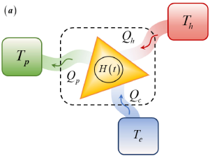
As shown schematically in Fig. 1(a), a FTQTC is established through a six-step process, directly inspired by its classical analogue (key-guoECM, ). The working substance is a two level system (TLS) with time-dependent Hamiltonian , where is the energy splitting at time , is the Pauli matrix in direction, and is Planck’s constant. The control protocol comprises three heat exchange steps during which the TLS is placed in thermal contact with reservoir , and three diabatic steps are characterized by sudden quench in the Hamiltonian.
A weak coupling between the system and reservoir is considered. The density operator of the TLS evolves according to the Markovian master equation, i,e., , where the generator represents the quantum Liouvillian superoperator. By considering that is finite but small enough and introducing the dimensionless time-rescaled parameter for a given reservoir , the first order approximation of the solution of the density operator is given by
| (1) |
where , with being the Drazin inverse of (key-Chenjf, ; key-Crook, ; key-Mandal, ), and the instantaneous Gibbs state with . The details of the calculation are reported in Appendix A. Based on Alicki’ s definition of heat (key-Alicki2016, ; key-Alicki2015, ) and Eq.(1), the amount of heat entering the system from reservoir during the interval (Appendix B)
| (2) |
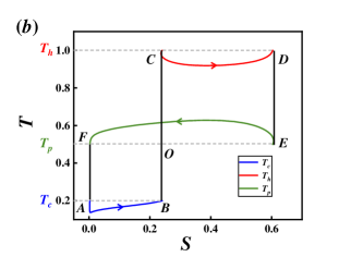
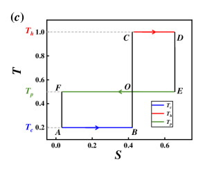
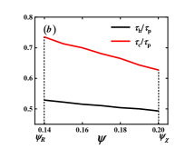
The zeroth order approximation of the density operator recovers the standard formula of heat in equilibrium thermodynamics, i.e., , where the entropy change of the equilibrium state of the system with . The first order irreversible corrections of heat with and . For a TLS, the Liouvillian superoperator , the instantaneous equilibrium state , and the Drazin inverse of the dissipator can be obtained from Appendix C, respectively. Figures 1(b) and (c) show the temperature-entropy diagram of an irreversible FTQTC and a reversible tricycle, respectively. The effective temperature of the TLS can be calculated by using the energy eigenbasis. It is given by the equation , where is the occupation probability of the ground state and is the occupation probability of the excited state. This equation is derived based on the assumption that the occupation probabilities follow the Boltzmann distribution (key-Quan, ). The entropy of a TLS can be calculated by using the density matrix formalism, which is given by . This entropy quantifies the amount of uncertainty or disorder in the TLS and is based on the von Neumann entropy, which is a measure of the system’s mixedness or lack of pure state. The detail of the control protocols of the quantum tricycle are designed as follows:
(1) Heat exchange with reservoir (from point A to B): When the TLS is coupled to reservoir with low-temperature , the time-modulated field drives the frequency of the TLS according to the cosine function in the time interval , where and denote the parameters of the amplitude and the displacement, respectively.
(2) Diabatic expansion (from point B to C): The system is isolated from any reservoir and the frequency suddenly shifted from to . The scaling factor is introduced, ensuring that the system continuously remains in equilibrium state during a reversible quantum tricycle. In addition, the rapidly changing condition of diabatic process prevents the TLS from adapting its configuration during the process, and thus the probability density remains unchanged.
(3) Heat exchange with reservoir (from point C to D): The system is coupled to reservoir with high-temperature in the time interval . The Hamiltonian of the system is concurrently modified by adjusting the frequency according to the function , where and signify the parameters of the amplitude and the displacement, respectively.
(4) First diabatic compression (from point D to E): The system is decoupled from the reservoir and a sudden quench is performed, in which the frequency is changed from into .
(5) Heat exchange with reservoir (from point E to F): An irreversible heat exchange process follows by coupling the system with reservoir at intermediate-temperature . The frequency of the system is slowly changed in accordance with the function in a time interval . The parameters and are the amplitude and the displacement in this process, respectively.
(6) Second diabatic compression (from point F to A): Finally, the system is disconnected from the reservoir and a sudden quench restores the frequency back to .
For a given heat exchange process, the time derivatives of at the beginning and the end of time are equal to zero, i.e., . This also gives rise to at and . Acccoring to Eq. (1), it guarantees that the system maintains the same equilibrium state both at the beginning and at the end of the heat exchange process. Furthermore, it ensures that the system remains in close proximity to the instantaneous steady state throughout the entire cycle. The selection of the scale parameter in frequency alteration during adiabatic operations enables a smooth transition of the system between the instantaneous equilibrium states associated with different reservoirs. With the given temperatures of , , and , as well as the values of , , and , we can deduce the following relationships: , , and (Appendix D).
Based on the the temperature-entropy diagram shown in Figs.1(b) and (c), it is observed that , , and , as , , and . In Ref. (key-PAbiuso, ), it is demonstrated that the first-order irreversible corrections of heat, i.e., . The sum of the first-order irreversible corrections of heat, represented by the expression , is less than or equal to zero. In addition, according to the principles of energy conversion, the sum of the heat entering a system in a cycle
| (3) |
Thus, the sum of the zeroth order approximation of heat . In a finite time cycle, it is true that , which implies that . As a result, the area of rectangle ABOF is not equal to the area of rectangle CDEO , as shown in Fig. 1(b).
In the case of a reversible cycle, a heat exchange process occurs over an infinitely extended duration, i.e., , leading to approaches zero. These quasi-static isothermal processes ensure that the system remains in thermal equilibrium with the heat source at all times. It follows from Eq. (3) that must be equal to zero. This leads to the equality between the area of rectangle ABOF and that of rectangle CDEO, as depicted in Fig. 1(c). At the quasistatic limit, and the coefficient of performance (COP) of the reversible cycle is then simplified as follows
| (4) |
III PERFORMANCE OPTIMIZATION IN THE SLOW-DRIVING REGIME
In the finite-time regime, the COP of the FTQTC can be calculated as
| (5) |
while the cooling rate is determined by the heat entering the TLS from reservoir divided by the total time required for cooling:
| (6) |
Here, the duration of the adiabatic process is significantly shorter than that of the heat exchange process and can be considered negligible. By utilizing Eqs. (5) and (6), we can generate performance characteristic curves for the cooling rate as a function of time and , as illustrated in Fig. 2. It is clearly seen from Fig. 2 that the cooling rate is not a monotonic function of time. The cooling rate can be improved by optimizing the durations of contact with heat reservoirs. Next, we consider the optimal configuration of the cycle in which the optimum cooling rate can be obtained under a given COP . By employing the Lagrangian method (key-Chenjincan1988, ; key-Wouagfack, ; key-Chenjincan1996, ), we can introduce
| (7) |
where and are the Lagrange multipliers associated with the given COP and the law of energy conservation, respectively. Form the Euler-Lagrange equations, we obtain
| (8) |
| (9) |
and
| (10) |
According to Eqs.(8-10) , the constraint equation of the times after eliminating the Lagrange multipliers is obtained by
| (11) |
In addition, we have another constraint equation for the time intervals derived from the energy conservation law as
IV RESULTS AND DISCUSSION
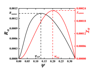
By substituting Eqs. (11) and (12) into Eqs. (5) and (6), we can generate the optimal curve of the cooling rate varying with the COP for given frequency exponent , as indicated by Fig. 3. The frequency exponent determines the spectral density of the bath. The specific relationship between and the first order correction of heat is elaborated in Appendix C. As depicted in Fig. 3, the cooling rate does not exhibit a monotonic behavior with respect to the COP. When , the cooling rate attains its local maximum value . The quantum refrigerator does not always operate at the state of the maximum cooling rate. In order to achieve both a higher COP and a larger cooling rate simultaneously, the refrigerator should be operated in the region of . However, when the refrigerator is operated in such a region, the cooling rate is a monotonically decreasing function of the COP.
It is a worth problem how to choose reasonably the cooling rate and the COP. The figure of merit , originally introduced by Yan and Chen (key-CJC1990, ),can be commonly employed as a target function for optimizing the performance of refrigerators (key-Tomas2012, ; key-Tu2012, ; key-PRE107044118(2023), ). By using Eqs. (5), (6), (11), and (12), we can plot the curves of as a function of for a given value of , as represented by the red solid curve in Fig. 3. It is observed from Fig. 3 that is not a monotonic function of for a given value of . When , attains its maximum . It is seen from Fig.3 that when , decreases with the decrease of . In general, the optimal range of should be determined by
| (13) |
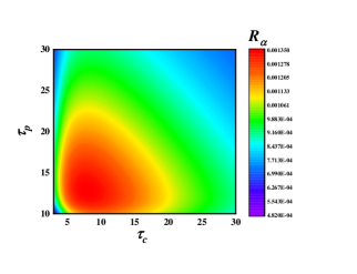
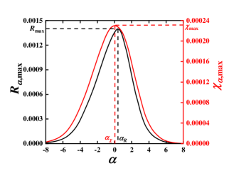
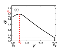
It can be found through the further analysis that both and are not monotonic functions of , as indicated by Fig.4. When , attains its maximum ; when , attains its maximum . Thus, the optimal range of should be
| (14) |
In the region of , both and decrease with the decrease of . In the region of , both and decrease with the increase of . The results obtained here offer a comprehensive framework for efficiently optimizing the control of a slowly driven FTQTC.
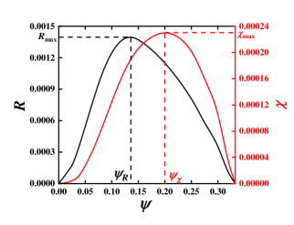
When is optimized, we can obtain the and optimum chararcteric curves, as shown in Fig.5. It is evident from Fig. 5 that the optimal range of the COP for a FTQTC is given by
| (15) |
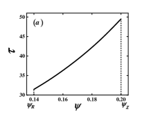
This is because both and decreases with the decrease of in the region of , while they decreases with the increase of in the region of . In the optimal region of , the total cycle time varies with for two given values and of , as shown in Fig. 6 (a), where two curves almost overlap. Similarly, we can plot the curves of and varying with , as shown in Fig. 6 (b), where two (or ) curves corresponding to two given values and of also almost overlap. It is observed from Fig.6 (a) and (b) that in the optimal region of , is a monotonically increasing function of , while and are monotonically decreasing functions of . However, is not a monotonic function of in the optimal region of , as indicated by Fig. 6(c). It is clearly seen from Fig. 6(c) or Eq. (11) that within three flat baths () are not the optimal selection for FTQTCs. When a FTQTC is operated within three flat baths, both the COP and the cooling rate are relatively small. This shows clearly that when the optimal performance of a FTQTC is researched, it is not enough to only study the performance of the FTQTCs operated within three flat baths.
V CONCLUSIONS
In this work, we presents a finite-time operaton for a quantum tricycle. The thermodynamic irreversibility during heat exchange processes is evaluated by analyzing the first-order irreversible corrections of heat using perturbation theory. The method of Lagrange multipliers has been employed to determine the optimal performances of the FTQTC. These configurations determine the cooling rate, the figure of merit, and the COP at the maximum cooling rate. The results demonstrate that, for a given spectrum of each bath, the values of the COP corresponding to the maximum figure of merit and the maximum cooling rate are different. To simultaneously achieve a relatively large cooling rate and COP, the performance of the FTQTCs can be improved by operating within the optimal range of states characterized by the frequency exponent.
APPENDIX A. SLOW DRIVING OF AN OPEN QUANTUM SYSTEM
In the case of an open quantum system, where the Hamiltonian contains a time-dependent parameter , and the system interacts with a reservoir at an inverse temperature , we assume that the evolution of the density operator is governed by the Markovian master equation,
| (16) |
By considering that the Liouvillian operator obeys the quantum detailed balance with respect to at all times, the Gibbs state becomes the immediate stationary state of Eq. (16), meaning that
| (17) |
As the modulation of frequency becomes infinitely slow, the dynamics of the system follow a quasi-static isothermal trajectory. During this trajectory, the system gradually adjusts to the instantaneous equilibrium state near the Gibbs ensemble . Substituting Eq. (17) into Eq.(16), we can derive an alternative evolution equation for as follows:
| (18) |
As is a traceless Hermitian operator, and the action of a superoperator on a traceless subspace is invertible (key-ScandiPHD, ), the solution of Eq. (18) can be expressed as follows:
| (19) |
where is the Drazin inverse of (key-Chenjf, ; key-Crook, ; key-Mandal, ). Therefore, the solution for Eq. (18) can be expanded in a series form through an iterative process. The expansion is given by the following expression:
| (20) |
Note that in Eq. (20), we have omitted the term with approaching infinity. This omission is justified by assuming that the derivative of the density operator with respect to time, when taken an infinite number of times, becomes zero.
We can rewrite Eq. (20) by introducing the dimensionless time-rescaled parameter as follows
| (21) |
where and . Rescaling the time provides the advantage of incorporating the duration of the evolution as a straightforward multiplicative factor in each term of the sum in Eq. (21). The state of the system now relies on the time within the unit interval , while the impact of the control protocol on the dynamics is encompassed within . Hence, Eq. (21) provides a perturbation expansion of the solution of the density operator in terms of powers of . During the finite-time slow driving process, there exists a lag between states and . Considering the first-order perturbation, we obtain Eq.(1) in the main text.
APPENDIX B. THERMODYNAMIC QUANTITY OF THE SLOWLY DRIVEN PROCESS
Building upon the derivation presented in the Appendix A, our objective is to investigate the impact of deviations from the corresponding quasistatic trajectory (as described in Eq. (1)) on the thermodynamic properties of the process. In order to accomplish this objective, it is important to observe that the mean energy and von Neumann entropy of system can be described by the following expressions as and , respectively. In a finite-time process with a duration of , the change in internal energy is typically divided into two components(key-Alicki2015, ; key-Alicki1979, ; key-Liufei, )
| (22) |
Employing Alicki’s definition of heat and considering the first-order perturbation in Eq. (1), we can determine the amount of heat that enters the system from the during the interval as follows:
| (23) |
where the time-rescaled Hamiltonian . In a quasi-static process that maintains the equilibrium state between the system and the bath, the zeroth-order approximation in equilibrium thermodynamics suggests that the system absorbs an amount of heat given by the expression:
| (24) |
Note that the entropy of the system in the equilibrium state is given by
| (25) |
Equation (24) is equivalent to
| (26) |
which is associated with the change in entropy along the quasi-static trajectory during the time interval . The first-order irreversible correction of heat
| (27) |
where
| (28) |
expresses the increase in dissipation that deviates from the reversible limit. Based on Appendixes A and B, the dynamics of the TLS under slow driving will be provided in Appendix C.
APPENDIX C. THE THERMODYNAMICS OF THE TLS UNDER SLOW DRIVING
Based on the aforementioned Appendixes, the calculation of the finite-time correction to the heat absorbed by a TLS is performed. In the weak coupling regime, the evolution of the system can be described by the Master Equation as follows:
| (29) |
Here, the damping rate relies on the coupling constant . The frequency exponent is determined by the spectral density of the bath (key-Cavina, ; key-Duan, ), which is assumed to be identical for all three baths. The value of characterizes the dissipation properties, categorizing it as a flat bath (), sub-Ohmic (), Ohmic (), or super-Ohmic () (key-Cangemi, ). The quantity represents the mean number of phonons associated with the bath at frequency . The notation denotes the anticommutator of the two operators. The operators and correspond to the raising and lowering operators, respectively.
The state of the TLS is expressed in terms of the density matrix as , where ( or ) represent the matrix elements of the density matrix. Further, the superoperator in the matrix form reads
| (30) |
At time , the instantaneous equilibrium state can be simplified as follows:
| (31) |
Therefore, the Drazin inverse is expressed as
| (32) |
By employing the time-rescaled parameter and utilizing the zeroth-order approximation in Eq.(24), the absorbed heat from bath can be estimated in the quasi-static limit. Furthermore, the first-order correction of the heat generated by the irreversible finite-time process can be calculated using Eq.(27), i.e.,
| (33) |
APPENDIX D. THE RELATIONSHIPS BETWEEN THE AMOLITUDE AND THE DISPLACEMENT
The choice of the parameters, amplitude and displacement , in the alteration of frequency during adiabatic operations enables the system to transition from the equilibrium state associated with one reservoir to the equilibrium state associated with another reservoir.
In the context of the quantum tricycle, it is necessary that the frequences of the TLS at the end of a heat exchange process and at the commencement of the subsequent heat exchange process are directly proportional to each other. Specifically, , , and . These requirements lead to the following relationships:
| (34) |
| (35) |
and
| (36) |
Employing Eqs. (34)-(36), in conjunction with the provided temperatures , , and , as well as the displacement values of and , and treating the amplitude parameter as the independent variable, we can deduce the following succinct relationships:
and
In the subsequent discussion, we can investigate an arbitrary quantum tricycle by varying the value of .
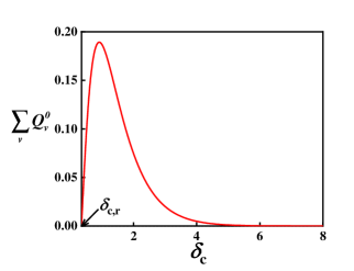
It is crucial to emphasize that the functioning of the cycle relies on the condition that the sum value of must be greater than or equal to zero, in accordance with the principles of energy conversion. The relationship curve in Fig. 7 depicts the variation of the sum of the zeroth-order approximation of heat as a function of the amplitude parameter . It is observed that the range of the amplitude parameter for a quantum tricycle is determined by . When , the sum of the zeroth-order approximation of heat is zero, indicating a reversible tricycle cycle. However, when , the sum of the zeroth-order approximation of heat is positive, indicating a finite-time irreversible tricycle cycle.
Acknowledgements.
This work has been supported by the National Natural Science Foundation (Grants No. 12075197),Natural Science Foundation of Fujian Province (Grant No. 2023J01006), and the Fundamental Research Fund for the Central Universities (No. 20720210024).References
- (1) R. Kosloff, Entropy, 19, 2100 (2013).
- (2) J. Chen and Z. Yan, J. Chem. Phys., 90, 4951 (1989).
- (3) C. Qi, L. Chen, Y. Ge, and H. Feng, J. Non-Equil. Thermody, 49, 11 (2024).
- (4) F. F. Huang, Engineering Thermodynamics (London, Macmillan,1976).
- (5) C. VandenBroeck, Phys. Rev. Lett. 95, 190602 (2005).
- (6) Y. Izumida and K. Okuda, Europhys. Lett. 97, 10004 (2012).
- (7) Y. Izumida and K. Okuda, New J. Phys. 17, 085011 (2015).
- (8) F. L. Curzon and B. Ahlborn, Am. J. Phys. 43, 22 (1975).
- (9) P. Salamon, A. Nitzan, B. Andresen, and R. S. Berry, Phys. Rev. A 21, 2115 (1980).
- (10) K. Sekimoto and S. Sasa, J. Phys. Soc. Jpn. 66, 3326 (1997).
- (11) M. Esposito, K. Lindenberg, and C. Van den Broeck, Europhys. Lett. 85, 60010 (2009).
- (12) M. Esposito, R. Kawai, K. Lindenberg, and C. Van den Broeck, Phys. Rev. E 81, 041106 (2010).
- (13) T. Schmiedl and U. Seifert, Europhys. Lett. 81, 20003 (2007).
- (14) Z. C. Tu, J. Phys. A: Math. Theor. 41, 312003 (2008).
- (15) Y. Izumida and K. Okuda, Europhys. Lett. 83, 60003 (2008).
- (16) Y. Izumida and K. Okuda, Phys. Rev. E 80, 021121 (2009).
- (17) Y. Izumida and K. Okuda, Eur. Phys. J. B 77, 499 (2010).
- (18) J. P. Pekola, Nat. Phys. 11, 118 (2015).
- (19) S. Vinjanampathy and J. Anders, Contemp. Phys. 57, 545 (2016).
- (20) F. Binder, L. A. Correa, C. Gogolin, J. Anders, and G. Adesso, Thermodynamics in the Quantum Regime, (Springer International Publishing, New York, 2018).
- (21) J. Chen and Z. Yan, J. Appl. Phys., 65, 1 (1989).
- (22) C. de Tomas, A. C. Hernandez, and J. M. M. Roco, Phys. Rev. E 85, 010104(R) (2012).
- (23) C. de Tomas, J. M. M. Roco, A. C. Hernandez, Y. Wang, and Z. C. Tu, Phys. Rev. E 87, 012105 (2013).
- (24) Y. Wang, M. Li, Z. C. Tu, A. C. Hernandez, and J. M. M. Roco, Phys. Rev. E 86, 011127 (2012).
- (25) J. Gonzalez-Ayala, A. Medina, J. M. M. Roco, and A. C. Hernandez, Phys. Rev. E 97, 022139 (2018).
- (26) V. Holubec and Z. Ye, Phys. Rev. E 101, 052124 (2020).
- (27) Z. Ye and V. Holubec, Phys. Rev. E 103, 052125 (2021).
- (28) J. Guo, H. Yang, H. Zhang, J. Gonzalez-Ayala, J. M. M. Roco, A. Medina, and A. C. Hernández, Energy Convers. Manage. 198, 111917 (2019).
- (29) Z. Li, J. Gonzalez-Ayala, H. Yang, J. Guo, and A. C. Hernández, J. Phys. A: Math. Theor. 55, 065001 (2022).
- (30) J. Guo, H. Yang, J. Gonzalez-Ayala, J. M. M. Roco, A. Medina, and A. C. Hernández, Energy Convers. Manage. 220, 113100 (2020).
- (31) A Levy and R Kosloff, Phys. Rev. Lett. 108, 070604 (2012).
- (32) D. Segal, Phys. Rev. E 97, 052145 (2018).
- (33) M. Kilgour and D. Segal, Phys. Rev. E 98, 012117 (2018).
- (34) F. Ivander, N. Anto-Sztrikacs, and D. Segal, Phys. Rev. E 105, 034112 (2022).
- (35) L. A. Correa, J. P. Palao, G. Adesso, and D. Alonso, Phys. Rev. E 87, 042131 (2013).
- (36) L. A. Correa, J. P. Palao, G. Adesso, and D. Alonso, Phys. Rev. E 90, 062124 (2014).
- (37) H. P. Breuer and F. Petruccione, The Theory of Open Quantum Systems (Oxford University Press, Oxford, 2002).
- (38) À. Rivas and S. F. Huelga, Open Quantum Systems: An Introduction (Springer, Heidelberg, 2012).
- (39) V. Cavina, A. Mari, and V. Giovannetti, Phys. Rev. Lett. 119, 050601 (2017).
- (40) P. Abiuso and M. Perarnau-Llobet, Phys. Rev. Lett. 124, 110606 (2020).
- (41) V. Singh and R. S. Johal, Phys. Rev. E 98, 062132 (2018).
- (42) M. Scandi and M. Perarnau-Llobet, Quantum 3, 197 (2019).
- (43) P. Abiuso, H. J. D. Miller, and M. Perarnau-Llobet, Entropy 22, 1076 (2020).
- (44) M. Scandi, Quantifying dissipation via thermodynamic length, Ph.D. thesis, Ludwig–Maximilians–Universität and Technische Universität München, 2018.
- (45) Y. H. Ma, R. X. Zhai, J. Chen, C. P. Sun, and H. Dong, Phys. Rev. Lett. 125, 210601 (2020).
- (46) J. F. Chen, C. P. Sun, and H. Dong, Phys. Rev. E 104, 034117 (2021).
- (47) J. Chen, Y. Wang, J. Chen, and S. Su, Phys. Rev. E 107, 044118 (2023).
- (48) E. Gavin, https://threeplusone.com/pubs/drazin03/.
- (49) D. Mandal and C. Jarzynski, J. Stat. Mech. 2016, 063204 (2016).
- (50) R. Alicki, J. Phys. A: Math. Theor. 49, 085001 (2016).
- (51) R. Alicki and D. Gelbwaser-Klimovsky, New J. Phys. 17, 115012 (2015).
- (52) H. T. Quan, Y. X. Liu, C. P. Sun, and F. Nori, Phys. Rev. E 76, 031105 (2007).
- (53) P. Abiuso, J. D. Miller, M. Perarnau-Llobet, and S. Matteo, Entropy, 22, 1076 (2020).
- (54) J. Chen and Z. Yan, J. Appl. Phys. 63, 4795 (1988).
- (55) P. A. N. Wouagfack and R. Tchinda, Renew. Sust. Energ. Revr. 21, 524 (2013).
- (56) J. Chen and C. Wu, Energ. Convers. Manage. 37, 353 (1996).
- (57) Z. Yan and J. Chen, J. Phys. D: Appl. Phys. 23, 136 (1990).
- (58) R. Alicki, J. Phys. A: Math. Gen. 12, L103 (1979).
- (59) F. Liu, Prog. Phys. 38, 1 (2018).
- (60) C. Duan, Z. Tang, J. Cao, and J. Wu, Phys. Rev. B 95, 214308 (2017).
- (61) L. M. Cangemi, G. Passarelli, V. Cataudella, P. Lucignano, and G. De Filippis, Phys. Rev. B 98, 184306 (2018).
- (62) T. L. Boullion and P. L. Odell. Generalised inverse matrices. Wiley-Interscience, New York, 1971.