Efficient Exact Algorithms for Minimum Covering of Orthogonal Polygons with Squares

Abstract

The Orthogonal Polygon Covering with Squares (OPCS) problem takes as input an orthogonal polygon without holes where vertices have integral coordinates i.e. a polygon $P$ without any holes, and with $n$ vertices and axis-parallel edges. Moreover, each vertex has integer-valued $x$- and $y$-coordinates. The aim is to find a minimum number of axis-parallel, possibly overlapping squares which lie completely inside $P$, such that their union covers the entire region inside $P$. Aupperle et. al [3] provide an $\mathcal{O}(N^{1.5})$-time algorithm to solve OPCS for orthogonal polygons without holes, where $N$ is the number of integral lattice points lying in the interior or on the boundary of $P$. Moreover, designing algorithms for OPCS with a running time polynomial in $n$ (the number of vertices of $P$) was discussed as an open question in [3], since $N$ can be exponentially larger than $n$. In this paper we design a polynomial-time exact algorithm for OPCS with a running time of $\mathcal{O}(n^{14})$.

We also consider the following structural parameterized version of the problem. A knob in an orthogonal polygon is a polygon edge whose both endpoints are convex polygon vertices. Given an input orthogonal polygon without holes that has $n$ vertices and $k$ knobs, we design an algorithm for OPCS with running time $\mathcal{O}(n^{2}+k^{14}\cdot n)$. This algorithm is more efficient than the above exact algorithm when $k=o(n^{13/14})$.

In [3], the Orthogonal Polygon with Holes Covering with Squares (OPCSH) problem is also studied. Here, the input is an an orthogonal polygon which could have holes and the objective is to find a minimum square covering of the input polygon. This version where the orthogonal polygon is allowed to have holes is shown to be NP-complete (even when all lattice points in the interior or on the boundary of the polygon constitute the input). We think there is an error in the existing proof in [3], where a reduction from Planar 3-CNF is shown. We fix this error in the proof with an alternate construction of one of the gadgets used in the reduction, hence completing the proof of NP-completeness of OPCSH, when all lattice points in the interior or on the boundary of the polygon are given as input.

1 Introduction

We consider the problem of covering orthogonal polygons with a minimum number of (possibly overlapping) axis-parallel squares.

An orthogonal polygon is a simple polygon such that every polygon-edge is parallel to either the x-axis or the y-axis (Figure 1(a)). We wish to cover a given orthogonal polygon with a minimum number of (possibly overlapping) axis-parallel squares, i.e. given an orthogonal polygon $P$ we wish to find a minimum number of squares such that every square lies inside the region of $P$ and the union of the regions of the plane covered by these squares is the region of the plane covered by polygon $P$ itself (Figure 1(b) and Figure 1(c)).

(a) Orthogonal Polygon

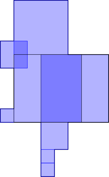
(b) Valid Covering

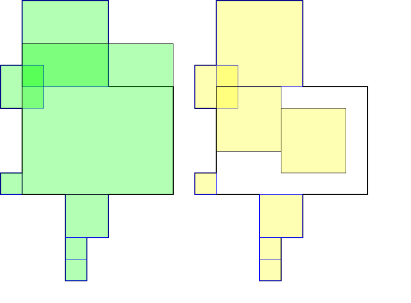
(c) Invalid Coverings. Left: A chosen square not contained in polygon (largest square in the diagram). Right: squares not covering entire polygon

Figure 1: Orthogonal Polygons and Covering with Squares

In general, an orthogonal polygon $P$ may contain holes. However, for most of the paper, we deal with problems where the input is an orthogonal polygon without any holes. First, we define the problem of Orthogonal Polygon Covering with Squares (OPCS) formally as follows.

Orthogonal Polygon Covering with Squares (OPCS) Input: An orthogonal polygon $P$ where its $n$ vertices have integral coordinates and $P$ does not have any holes Question: Find the minimum number of axis-parallel squares contained in $P$, such that $P$ is entirely covered by these squares

Note that for this problem, it is possible that the input polygon is given in terms of its $n$ vertices and their coordinates. Since the polygon is such that all vertices have integral coordinates, it is also possible that the input polygon is given in terms of its boundary vertices as well as all lattice points contained inside $P$. Let this set of lattice points lying on the boundary of $P$ or inside $P$ be of size $N$. Note that there could be an exponential factor difference between the values of $N$ and $n$.

We also study a parameterized version of OPCS, called $p$-OPCS. Before we define the problem, let us consider a knob as a structure occurring in an orthogonal polygon $P$. A knob is an edge where both endpoints are convex vertices of $P$ (the formal definition of knobs is given in Section 2).

$p$-Orthogonal Polygon Covering with Squares ($p$-OPCS) Parameter: $k$ Input: An orthogonal polygon $P$ where its $n$ vertices have integral coordinates and $P$ does not have any holes, a non-negative integer $k$ such that $P$ has at most $k$ knobs Question: Find the minimum number of axis-parallel squares contained in $P$, such that $P$ is entirely covered by these squares

The parameterized problem of $p$-OPCS takes the number of knobs in the input orthogonal polygon to be a structural parameter, to be utilized when designing parameterized algorithms.

The final variant that we consider in this paper is the following variant of OPCS where the input orthogonal polygon is allowed to have holes.

Square Covering of Orthogonal Polygons with Holes (OPCSH) Input: An orthogonal polygon $P$ (possibly with holes) where all boundary vertices have integral coordinates Question: Find the minimum number of axis-parallel squares contained in $P$, such that $P$ is entirely covered by these squares

Once again, the polygon $P$ could be described in terms of its $n$ boundary vertices, or in terms of the $N$ lattice vertices that lie on the boundary of $P$ or inside $P$.

Previous Results.

The OPCS problem originates from image processing and further finds its application in VLSI mask generation, incremental update of raster displays, and image compression [9]. Moitra [9] considers the problem of a minimal covering of squares (i.e. no subset of the cover is also a cover) for covering a binary image $\sqrt{N}\times\sqrt{N}$ pixels; and presents a parallel algorithm running on EREW PRAM which takes time $T\in[\log N,N]$ with $(N/T)$ processors.

In [3], exact polynomial time solutions of OPCS are discussed, where the input is considered to be the set of all $N$ lattice points inside (in the interior and the boundary of) $P$. The algorithms crucially use following associated graph $G(P)$.

Definition 1.1 (Associated graph $G(P)$).

A unit square region inside an orthogonal polygon $P$ with corners on lattice points is called a block. An associated graph $G(P)$ is constructed with the set of nodes as the set of blocks inside $P$; two blocks $p_{1}$ and $p_{2}$ are connected by an undirected edge if there is an axis parallel square lying inside $P$ that simultaneously covers $p_{1}$ and $p_{2}$.

Clearly from the definition, we know that any set of blocks covered simultaneously by a single square shall form a clique. Further, [1] shows the converse as well.

Proposition 1.2.

A subset of blocks inside an orthogonal polygon $P$ can be covered by a square if and only if they induce a clique in $G(P)$.

In [3], $G(P)$ is shown to be a chordal graph (please refer to Definition 2.13 for the definition of a chordal graph) if $P$ does not have holes. In [3] it is further shown that using the polynomial time algorithm for minimum clique covering in chordal graphs (discussed in [7]), OPCS can be solved in polynomial time. If the number of lattice points inside $P$ is $N$, then the algorithm takes $\mathcal{O}(N^{2.5})$ time. In [3], there is also references provided that would result in an algorithm with complexity $\mathcal{O}(N^{1.5})$ to solve minimum clique cover in the associated chordal graph $G(P)$ using more structural properties of the orthogonal polygon $P$.

Aupperle et. al [3] also prove that OPCSH is NP-Hard if the input orthogonal polygon $P$ with possible holes is described in terms if the $N$ lattice points lying on the boundary of $P$ as well as inside $P$. The paper reduces Planar 3-CNF [8] to this problem in order to prove its NP-Hardness.

Bar-Yehuda [4] describes an $\mathcal{O}(n\log n+\textsc{OPT})$ $2$-factor approximation algorithm to solve this problem where $n$ is the number of vertices and OPT is the minimum number of squares to cover $P$.

Culberson and Reckhow [6] proves that the problem of minimum covering of orthogonal polygons with rectangles is NP-hard. Kumar and Ramesh [2] provide a polynomial time approximation algorithm with approximation factor of $\mathcal{O}(\sqrt{\log N})$ for the problem of covering orthogonal polygons (with or without holes) with rectangles. Most of the other geometric minimum cover problems for orthogonal polygons are NP-complete as well [10].

Our Results.

In the results due to [3], the input size is considered to be the number of lattice points inside $P$ or lying on the boundary of $P$. However, it is inefficient to represent orthogonal polygons with all the lattice points inside it. Rather, it would be more efficient to take an orthogonal polygon $P$ as a sequence of the boundary vertex points of $P$ (in either clockwise or counter-clockwise direction). In case $P$ has one or more holes, then this kind of input lists the sequence of vertices on the outer boundary, followed by the sequence of vertices on the boundary of each hole of $P$.

As an example, if $P$ is itself a large square with vertices $(0,0)$, $(0,2^{t})$, $(2^{t},0)$, $(2^{t},2^{t})$, then even though it can be represented by just $O(t)$ bits by simply listing down the vertices in order, we would need $\Omega(4^{t})$ bits to actually represent all lattice points that lie inside or on the boundary of $P$. Moreover, if OPT is the actual minimum number of squares to completely cover $P$, $OPT$ can also potentially be exponential in the number of bits needed to represent the vertices (e.g. $P$ is a $1\times 2^{t}$ rectangle).

In this paper we consider the input size $n$ as the number of polygon vertices of $P$ and then design efficient algorithms for minimum square covering with respect to $n$. Note that the algorithm in [3] becomes exponential now, as there can be exponentially many points inside $P$. Designing algorithms which are polynomial in the number $n$ of polygon vertices was stated as an open question in [3]. To the best of our knowledge, this is the first study to answer these questions. This algorithm with a running time of $\mathcal{O}(n^{14})$, where $n$ is the number of vertices of the input polygon, and related structural results are given in Section 3 and Section 4. Moreover, our algorithm also works for polygons with rational coordinates as we can simply scale up the polygon by an appropriate denominator without changing the number of vertices $n$.

In Section 5, we consider the $p$-OPCS problem and further optimize the above algorithm, considering the polygon to have $n$ vertices and $k$ knobs (edges with both endpoints subtending $90^{\circ}$ to the interior of the polygon, formally defined in Definition 2.1). We design a recursive algorithm running in time $\mathcal{O}(n^{2}+k^{14}\cdot n)$. This algorithm is more efficient than the above exact algorithm if $k=o(n^{13/14})$.

Finally in Section 6, we fix an error in the proof discussed in [3] of NP-completeness of minimum square covering of orthogonal polygons with holes. Note that such a result implies that we do not expect an algorithm for OPCSH that has a running time polynomial in the number $n$ of boundary vertices of the input orthogonal polygon $P$ which may have holes.

All other notations and definitions used in the paper can be found in Section 2.

2 Preliminaries

Orthogonal Polygons.

We denote by $P$ our input polygon with $n$ vertices. In the entire paper, we always consider the vertices of the polygon to have integral coordinates. Unless mentioned otherwise, the polygon $P$ is assumed to not have any holes. Let the vertices of $P$ in order be $v_{1},v_{2},\ldots,v_{n}$, where $v_{i}=(x_{i},y_{i})$ with $x_{i}$ and $y_{i}$ being integer coordinates. For convenience, we define $v_{0}:=v_{n}$ and $v_{n+1}:=v_{1}$. Therefore $(v_{i},v_{i+1})$ is a polygon edge of $P$ for all $i\in\{1,2,\ldots,n\}$. For any natural number $d$, we denote the set $\{1,2,\ldots,d\}$ by the notation $[d]$. Next, let the minimum number of squares required to cover $P$ be denoted by $\textsc{{OPCS}}(P)$. We use the terms left, right, top, bottom, vertical, horizontal to indicate greater x-coordinate, smaller x-coordinate, greater y-coordinate, smaller y-coordinate, parallel to y-axis, and parallel to x-axis, respectively. By boundary of a square (rectangle), we mean its four sides. A block lying on the boundary of a square is one which lies inside the square and where the boundary of the block overlaps with the boundary of the square. We assume that arithmetic and logic operations on two numbers take constant time. For any two points $a$, $b$ on the plane, we denote the (Euclidean) length of the line segment joining $a$ and $b$ as $\overline{ab}$.

Given an input polygon $P$ of OPCS, the minimum number of squares to cover $P$ remains the same, even if $P$ is scaled up by an integral factor and/or rotated $90^{\circ}$ (clockwise/counter-clockwise).

Let us formally define convex and concave vertices of an orthogonal polygon.

Definition 2.1 (Concave and Convex vertices of $P$).

A vertex $v_{i}$ of an orthogonal polygon $P$ is a convex vertex if $v_{i}$ subtends an angle of $90^{\circ}$ to the interior of $P$. A vertex $v_{j}$ of $P$ is a concave vertex if it subtends an angle of $270^{\circ}$ to the interior of $P$(Figure 2).

Figure 2: Convex vertices: $\{v_{1},v_{2},v_{3},v_{5},v_{6},v_{8},v_{10},v_{12},v_{13}\}$, concave vertices: $\{v_{4},v_{7},v_{9},v_{11},v_{14}\}$

For the OPCS problem, we are only interested in maximal squares that are completely contained in the region of the input polygon.

Definition 2.2 (Valid Square).

An axis parallel square $S$ is called a valid covering square of of an orthogonal polygon $P$ or simply a valid square if $S$ is fully contained in the region of $P$.

Definition 2.3 (Maximal Square).

A valid square $S$ is a maximal valid square or simply a maximal square, if no other valid square with a larger area contains $S$ entirely(Figure 3).

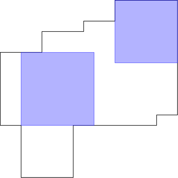
(a) Some maximal squares

(b) Valid squares which are not maximal

Figure 3: Orthogonal Polygons and Covering with Squares

Note that for a given minimum square covering of an input orthogonal polygon $P$, some squares may be maximal squares (Definition 2.2) while the other squares may be valid squares which are not maximal. However, for each such valid square $S$ which is not maximal, we can replace it with any maximal square containing $S$ (this exists as $S$ is not maximal and the interior of $P$ is a bounded region with finite area) to obtain another minimum square covering of $P$. Since this process does not change the count of the squares used to cover $P$ and since the newly introduced squares cover the entire area of the removed squares, the new covering is a minimum covering with maximal squares. There exists a minimum square covering of any orthogonal polygon $P$ where every square of the covering is a maximal square.

The paper [3] defines a structure called knobs. We define knobs slightly differently but they essentially are the same.

Definition 2.4 (Knob).

A knob in an orthogonal polygon $P$ is an edge $(v_{i},v_{i+1})$ of $P$ such that $v_{i}$ and $v_{i+1}$ are both convex vertices of $P$ (Figure 4(a)). Suppose $v_{i}$ and $v_{i+1}$ share the same x coordinate. Then we say that they form a left knob if $(v_{i},v_{i+1})$ is a left boundary edge (i.e. all points just to the left of the edge are in the exterior of $P$), otherwise they form a right knob. Similarly, when $v_{i}$ and $v_{i+1}$ share the same y coordinate, then we say that they form a top knob if $(v_{i},v_{i+1})$ is a top boundary edge (i.e. all points just to the top of the edge are in the exterior of $P$), otherwise they form a bottom knob.

Next, we define a non-knob convex vertex.

Definition 2.5 (Non-Knob Convex Vertex).

Given an orthogonal polygon $P$, a convex vertex $v_{i}$ is said to be a non-knob convex vertex if neither $(v_{i},v_{i+1})$ nor $(v_{i-1},v_{i})$ is a knob (i.e. both $v_{i-1}$ and $v_{i+1}$ are concave vertices).

We further introduce strips as follows.

Definition 2.6 (Strip).

A strip of an orthogonal polygon $P$ is a maximal axis-parallel non-square rectangular region $Y$ lying inside $P$ such that each side in the longer set of parallel sides of $Y$ is contained entirely in a polygon edge of $P$ (Figure 4(b)).

(a) $(v_{t},v_{t+1})$ is a top knob, $(v_{l},v_{l+1})$ is a left knob, $(v_{r},v_{r+1})$ is a right knob, $(v_{b},v_{b+1})$ is a bottom knob

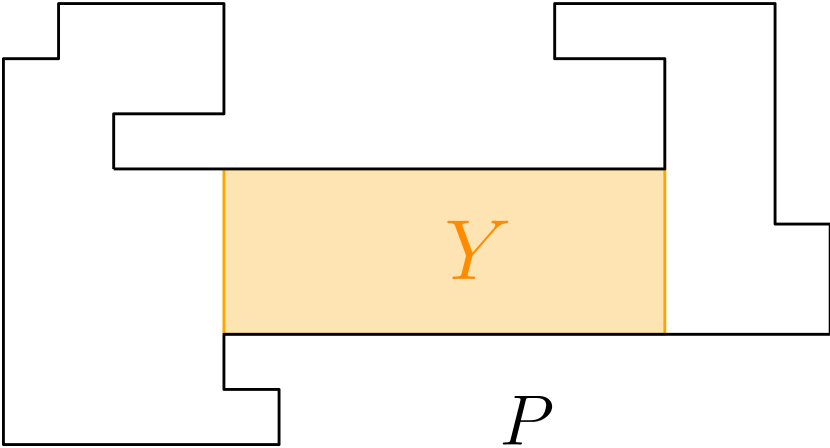
(b) Strip $Y$ of the polygon $P$

Figure 4: Knobs and Strips

We make the following observation

Given an orthogonal polygon $P$, for any pair of parallel polygon edges $e_{1}$, $e_{2}$, there can be at most one strip with its longer sides lying inside $e_{1}$ and $e_{2}$ respectively.

Efficient Representation of Squares.

We introduce the following notations to represent a sequence of squares placed side by side. We start by defining a rec-pack, which is a $t\times\eta t$ or $\eta t\times t$ rectangle lying inside the given orthogonal polygon $P$, where $\eta\in\mathbb{N}$.

Definition 2.7 (Rec-pack).

Given an orthogonal polygon $P$, a rec-pack of $P$ is an axis parallel rectangle $R$ (of dimension $t\times\eta t$ or $\eta t\times t$) with integer aspect ratio $\eta$ (i.e. ratio of the lengths of the longer side to its shorter side) that lies completely inside $P$ (Figure 5(a)). We define the length $t$ of the shorter side of the rec-pack $R$ to be the width of $R$ and the aspect ratio $\eta$ to be the strength of $R$.

Remark 2.8.

A valid square is a rec-pack of strength $1$. We consider any square to be a trivial rec-pack.

For a rec-pack $R$ with width $t$ and strength $\eta$, it can be covered with exactly $\eta$ many $t\times t$ valid squares. We formally define this operation in the next definition.

Definition 2.9 (Extraction of rec-pack).

Given an orthogonal polygon $P$ and a rec-pack $R$ of width $t$ and strength $\eta$ in $P$, we define the extraction of $R$, $\mathcal{E}(R)$ to be the sequence of $\eta$ valid squares of size $t\times t$ placed side by side to cover the entire region of $R$ (Figure 5(b)). Moreover, for a set of rec-packs $\mathcal{R}$, we define its extraction $\mathcal{E}(\mathcal{R})$ to be the union of the extraction of each rec-pack in $\mathcal{R}$.

$$\mathcal{E}(\mathcal{R})=\bigcup\limits_{R\in\mathcal{R}}\mathcal{E}(R)$$

(a) Rec-pack $R$ with strength $4$

(b) Extraction $\mathcal{E}(R)$ of rec-pack $R$

Figure 5: Rec-packs and Extractions

Remark 2.10.

For a square $S$ (a trivial rec-pack), the extraction is a singleton set containing $S$ itself, i.e. $\mathcal{E}(S)=\{S\}$. Moreover, for any set $\mathcal{S}$ of squares, we have $\mathcal{E}(\mathcal{S})=\mathcal{S}$.

Note that any side-by-side placed sequence of $\eta$ many $t\times t$ valid squares covers up a rec-pack of width $t$ and strength $\eta$. Therefore, whenever there is a solution with a side-by-side placed sequence of congruent squares, we can keep track of the rec-pack which gives the set of these congruent squares upon extraction. But first, we need to define a covering using rec-packs.

Definition 2.11.

A set of rec-packs $\mathcal{R}$ is said to cover the input orthogonal polygon $P$ if the set of squares in $\mathcal{E}(\mathcal{R})$ cover the polygon $P$. Moreover, we say $\mathcal{R}$ to be a minimum covering, if $\mathcal{E}(\mathcal{R})$ is a minimum cardinality set of squares covering $P$ and no two rec-packs $R_{1},R_{2}\in\mathcal{R}$ have $\mathcal{E}(R_{1})\cap\mathcal{E}(R_{2})\neq\emptyset$ (i.e. produce some common square).

Remark 2.12.

For any set $\mathcal{S}$ of squares covering $P$, $\mathcal{S}$ is also a set of rec-packs covering $P$. Similarly, for any minimum cardinality set of squares $\mathcal{S}$ covering $P$, $\mathcal{S}$ is also a set of rec-packs which is a minimum covering of $P$. Finally, if a set of rec-packs $\mathcal{R}$ is a covering (minimum covering) of $P$, then the set of squares $\mathcal{E}(\mathcal{R})$ is a set of trivial rec-packs which is also a covering (minimum covering).

We also state the following observation.

A set of rec-packs $\mathcal{R}$ covers an orthogonal polygon $P$ if and only if all the rec-packs in $P$ together form a set of rectangles covering $P$.

Graph Theory.

Given a graph $G$, we denote the vertex set by $V(G)$ and the edge set by $E(G)$. The neighbourhood of a vertex $v\in V(G)$ is denoted by $N(v)$. The closed neighbourhood of $v$ is denoted by $N[v]$. Given a graph $G$, a subgraph $H$ is an induced subgraph of $G$ if $V(H)\subseteq V(G)$ and $E(H)$ contains all edges of $E(G)$ such that both endpoints are in $V(H)$. In this case, we also say that the vertex set $V(H)$ induces the subgraph $H$. Recall the definition of chordal graphs and simplicial nodes [5].

Definition 2.13 (Chordal graphs and simplicial nodes).

A chordal graph $G$ is a simple graph in which every cycle of length at least four has a chord. A node $v\in V(G)$ is simplicial if $N[v]$ induces a complete graph.

We get the following result directly from the definition.

Proposition 2.14.

Any induced subgraph of a chordal graph is also chordal.

We now state Dirac’s Lemma on chordal graphs [5].

Proposition 2.15 (Dirac’s Lemma).

Every chordal graph has a simplicial node. Morever, if a chordal graph is not a complete graph, it has at least two non-adjacent simplicial nodes.

We finally reiterate one of the major results of [3].

Proposition 2.16.

For a simple orthogonal polygon $P$ (without holes), the associated graph $G(P)$ is chordal.

3 Structural and Geometric Results

In this section, we prove some structural and geometric results of a minimum square covering of an orthogonal polygon $P$, as well as a set of rec-packs which is a minimum covering of $P$.

3.1 Structure of Minimum Coverings

Due to Figure 3 we assume that we are looking for a minimum covering where every square is a maximal square. First, let us define how a maximal square can be obtained from a convex vertex of the given orthogonal polygon $P$.

Definition 3.1.

Given an orthogonal polygon $P$ and a point $v$, the following process is called growing of a square with one corner fixed at $v$:

• start with $S_{1}$ being the $1\times 1$ valid square covering $v$ (and has $v$ as one of its corners).

• for $t$ in $2,3,\ldots$, from $S_{t-1}$, which is a $(t-1)\times(t-1)$ square with $v$ as one of its corners, construct $T$ to be a $t\times t$ square by keeping one of its vertex fixed at $v$ and changing both the $x$- and $y$-coordinates of the diagonally opposite vertex in $S_{t-1}$ by $1$ to obtain the corresponding diagonally opposite vertex in $T$. If $T$ is a valid square, set $S_{t}\leftarrow T$; else terminate the process and set $S=S_{t-1}$.

$S$ is said to be the square grown from the point $v$.

We now discuss the following result.

Lemma 3.2.

Given an orthogonal polygon $P$, the maximal square covering a convex vertex is unique. Further, for a given convex vertex $v$, the unique maximal square can be found in $\mathcal{O}(n)$.

Proof 3.3.

Given a convex vertex $v$ in an orthogonal polygon $P$, let $S$ be the vertex grown from $v$. As all other squares covering $v$ strictly lie inside $S$, $S$ must be the unique maximal square covering $v$.

Let $\mathcal{R}$ denote the region defined by the interior of the $90^{\circ}$ angle between the rays formed by extending the two edges adjacent to $v$ (i.e. a quadrant). To find $S$ in $\mathcal{O}(n)$ time, we can iterate over all polygon edges $(v_{i},v_{i+1})$, and check the following:

• if $(v_{i},v_{i+1})$ lies entirely outside $\mathcal{R}$, it can never constrain the maximal square covering $v$, so we continue to the next iteration

• if some portion of $(v_{i},v_{i+1})$ lies inside $\mathcal{R}$, then find in $\mathcal{O}(1)$, the largest square in $\mathcal{R}$, with one vertex at $v$ and the strict interior of the square does not contain any portion of $(v_{i},v_{i+1})$. This can be done in $\mathcal{O}(1)$, just by comparing the coordinates of $v_{i}$, $v_{i+1}$ and $v$.

Finally, the square with the minimum area is the unique maximal square covering $v$, as all other edges allow larger (or equally large) squares.

We now define a maximal corner square of a vertex as follows.

Definition 3.4 (Maximal Corner Square of a vertex).

The Maximal Corner Square of a convex vertex $v$, or $MCS(v)$ is the unique maximal square covering $v$.

Remark 3.5.

Due to Proposition 3 and Lemma 3.2, there is a minimum square covering of an orthogonal polygon $P$ such that for each of the convex vertices $v$, $MCS(v)$ is one of the squares in the minimum covering.

Note that any maximal square should be bounded by either two vertical polygon edges or two horizontal polygon edges.

Lemma 3.6.

If $S$ is a maximal square of an orthogonal polygon $P$, then either both the vertical sides of $S$ overlap fully or partially with some polygon edges in $P$ or both the horizontal sides of $S$ overlap fully or partially with some polygon edges of $P$.

Proof 3.7.

Assume the contrary. Suppose for some maximal square $S$ there is one horizontal edge and one vertical edge which does not overlap fully or partially with any polygon edges of $P$. Further, we can assume that these are the top and the right edges of $S$ (we can rotate $P$ along with $S$ appropriately if this is not the case). Then we can further grow $S$ fixing its bottom-left corner, which contradicts that $S$ is a maximal square.

3.2 Simplicial Nodes in the Associated Graph and Partial Solutions

We define a partial solution for OPCS to be a subset of a set of rec-packs which is a minimum covering of $P$.

Definition 3.8 (Partial Solution).

Given an orthogonal polygon $P$, a set of rec-packs $\mathcal{R}$ is a partial solution for OPCS if there is a minimum covering set of rec-packs $\mathcal{R}^{\prime}$ with $\mathcal{R}\subseteq\mathcal{R}^{\prime}$.

Now consider a partial solution $\mathcal{R}$. We define $G^{\mathcal{R}}(P)$ as follows.

Definition 3.9.

Let $G^{\mathcal{R}}(P)$ denote the induced subgraph of the associated graph $\mathcal{G}(P)$ consisting of nodes which correspond to blocks in $P$ which are not covered by any rec-pack in $\mathcal{R}$.

From Proposition 2.16 and Proposition 2.14, we get that $G^{\mathcal{R}}(P)$ is chordal, and from Proposition 2.15 we get that $G^{\mathcal{R}}(P)$ has a simplicial node $p$ if $G^{\mathcal{R}}(P)$ is non-empty. Let $A$ denote the union of the block $p$ and its neighbouring blocks in $G^{\mathcal{R}}(P)$. By Definition 2.13, $A$ induces a clique in $G^{\mathcal{R}}(P)$ and hence in $G(P)$. Therefore, by Proposition 1.2, there exists a maximal square $S_{A}$ that covers all blocks in $A$. Next, we define unambiguous squares given a partial solution $\mathcal{R}$.

Definition 3.10 (Unambiguous squares given a partial solution).

Let $\mathcal{R}$ be a partial solution for OPCS in an orthogonal polygon $P$. We call a maximal square $S$ to be an unambiguous square given $\mathcal{R}$, if there is simplicial node $p$ in $G^{\mathcal{R}}(P)$ such that $S$ covers $p$ and all its neighbours in $G^{\mathcal{R}}(P)$.

Remark 3.11.

For a given simplicial node $p$ in $G^{\mathcal{R}}(P)$, there can be multiple maximal squares that cover $p$ and all its neighbours in $G^{\mathcal{R}}(P)$.

We now justify the naming of unambiguous squares.

Lemma 3.12.

If $\mathcal{R}$ is a partial solution for OPCS in an orthogonal polygon $P$ and $S$ is an unambiguous square given $\mathcal{R}$, then $\mathcal{R}\cup\{S\}$ is also a partial solution.

Proof 3.13.

Let $p$ be a simplicial node in $G^{\mathcal{R}}(P)$ such that $S$ covers $p$ and its neighbours in $G^{\mathcal{R}}(P)$. Since $\mathcal{R}$ is a partial solution, there exists a minimum cover $\mathcal{R}^{\prime}$ covering $P$ with $\mathcal{R}\subseteq\mathcal{R}^{\prime}$. This implies $\mathcal{E}(\mathcal{R})\subseteq\mathcal{E}(\mathcal{R}^{\prime})$ from Definition 2.9. Let $S^{\prime}\in\mathcal{E}(\mathcal{R}^{\prime})$ be a maximal square covering $p$. We have $S^{\prime}\notin\mathcal{E}(\mathcal{R})$ as $p$ is in $G^{\mathcal{R}}(P)$. This implies that $\mathcal{E}(\mathcal{R})\subseteq\mathcal{E}(\mathcal{R}^{\prime})\setminus\{S^{\prime}\}$. However, since $S^{\prime}$ covers an induced clique of $G^{\mathcal{R}}(P)$ including $p$ (Proposition 1.2) and possibly some blocks already covered by squares in $\mathcal{E}(\mathcal{R})$, this means that $S^{\prime}$ covers $p$ and a subset of its neighbours in $G^{\mathcal{R}}(P)$ along with some blocks already covered by squares in $\mathcal{E}(\mathcal{R})$. On the other hand, recall that $S$ covers $p$ and all its neighbours in $G^{\mathcal{R}}(P)$. This means $\mathcal{E}(\mathcal{R})\cup\{S^{\prime}\}$ covers a subset of points covered by $\mathcal{E}(\mathcal{R})\cup\{S\}$. This means $(\mathcal{E}(\mathcal{R}^{\prime})\setminus\{S^{\prime}\})\cup\{S\}$ is also a minimum cardinality set of squares covering the entire polygon $P$. Let $\mathcal{Z}=(\mathcal{E}(\mathcal{R}^{\prime})\setminus\{S^{\prime}\})\cup\{S\}$.

We rewrite $\mathcal{Z}=(\mathcal{E}(\mathcal{R}^{\prime})\setminus\{S^{\prime}\})\cup\{S\}=(\mathcal{E}(\mathcal{R})\cup\mathcal{T})\cup\{S\}$, where $\mathcal{T}=(\mathcal{E}(\mathcal{R}^{\prime})\setminus\{S^{\prime}\})\setminus\mathcal{E}(\mathcal{R})$. Consider $\mathcal{Z}_{1}=\mathcal{R}\cup\mathcal{T}\cup\{S\}$ to be a set of rec-packs (where $\mathcal{T}$ and $\{S\}$ are considered to be sets of trivial rec-packs). Since $\mathcal{E}(\mathcal{Z}_{1})=\mathcal{E}(\mathcal{R}\cup\mathcal{T}\cup\{S\})=\mathcal{E}(\mathcal{R})\cup\mathcal{T}\cup\{S\}=\mathcal{Z}$ is a minimum cardinality set of squares covering $P$, $\mathcal{Z}_{1}$ is a minimum covering. Moreover, as $\mathcal{R}\cup\{S\}\subseteq\mathcal{Z}_{1}$, $\mathcal{R}\cup\{S\}$ is a partial solution. Hence, we are done.

Now, we prove that we can always find an unambiguous square which follows a particular structure.

Lemma 3.14.

Let $\mathcal{R}$ be a partial solution of OPCS in an orthogonal polygon $P$ such that $\mathcal{E}(\mathcal{R})$ does not completely cover $P$. We define $C_{x}$ and $C_{y}$ as a set of lattice points as follows.

$$C_{x}:=\{ (x,y)\in\mathbb{Z}^{2}|x\text{ is an x-coordinate of a vertex of }P,$$

$$y\text{ is a y-coordinate of a vertex of }P\text{ or a corner of a rec-pack in }\mathcal{R}\}$$

$$C_{y}:=\{ (x,y)\in\mathbb{Z}^{2}|x\text{ is an x-coordinate of a vertex of }P\text{ or a corner of a rec-pack in }\mathcal{R},$$

$$y\text{ is a y-coordinate of a vertex of }P\}$$

Then there exists an unambiguous square $S$ given $\mathcal{R}$ which has one corner in $C_{x}\cup C_{y}$.

Proof 3.15.

Let $p$ be a simplicial node in $G^{\mathcal{R}}(P)$ with the largest number of neighbours, and such that among the topmost such simplicial nodes it is the leftmost. Let $A$ denote the following set of nodes (blocks in $P$): $p$ and its neighbours in $G^{\mathcal{R}}(P)$. Let $S_{0}$ be a maximal square that covers all blocks in $A$, such that the position of the top-left corner of $S_{0}$ is leftmost among the topmost of all such squares covering $A$. By Lemma 3.6, we know that either the horizontal sides of $S_{0}$ overlaps (completely or partially) with two horizontal polygon edges, or the vertical sides of $S_{0}$ overlaps (completely or partially) with two vertical polygon edges.

Assume that the horizontal sides of $S_{0}$ overlaps (completely or partially) with two horizontal polygon edges. We consider two cases.

Case-I: $S_{0}$ is a $1\times 1$ square.

Since $p$ is a simplicial node with the largest number of neighbours in $G^{\mathcal{R}}(P)$, all simplicial nodes (in fact all nodes) in $G^{\mathcal{R}}(P)$ must be isolated. Further, $p$ is the leftmost among the topmost such simplicial nodes. This means that the immediate left block $p^{\prime}$ of $p$ is either covered by a rec-pack in $\mathcal{R}$ or is outside the polygon. Therefore, the left side of $S_{0}$ is either a polygon edge (if $p$ is in the polygon but $p^{\prime}$ is not) or a vertical side of some rec-pack in $\mathcal{R}$ (if $p$ is uncovered, but $p^{\prime}$ is covered), respectively. Therefore, the top-left corner of $S_{0}$ must share the x-coordinate of either a corner of a rec-pack in $\mathcal{R}$ or a polygon vertex. Further, the top-left corner of $S_{0}$ shares a y-coordinate of a polygon vertex as the horizontal sides (top and bottom) of $S_{0}$ overlap with polygon edges. This means that the top-left vertex of $S_{0}$ is in $C_{y}$

Case-II: $S_{0}$ is not a $1\times 1$ square.

We already know that the horizontal sides (top and bottom) of $S_{0}$ overlap with polygon edges. If the left (or right) side of $S_{0}$ shares x-coordinate of some polygon edge or a corner of some rec-pack in $\mathcal{R}$, then the top-left (or top-right) corner of $S_{0}$ is in $C_{y}$; and then we are done.

Now, we assume the contrary. Suppose neither the left or right sides of $S_{0}$ share an x-coordinate with a polygon edge or a corner of some rec-pack in $\mathcal{R}$. In particular, if $S_{l}$ and $S_{r}$ are squares congruent to $S_{0}$ but are shifted one unit to the left and right respectively, then $S_{l}$ and $S_{r}$ are maximal valid squares (Figure 6(a)). They are valid as the left and right sides of $S_{0}$ do not overlap with any polygon edge. They are also maximal as the same polygon edges overlapping horizontal sides of $S_{0}$ also overlap the horizontal sides of $S_{l}$ and $S_{r}$ (this would not be the case if the horizontal polygon edges only overlap horizontal sides of $S_{0}$ at just a point — i.e. a corner of $S_{0}$ overlaps with a vertex of $P$; but then the vertical side of that corner of $S_{0}$ would share the x-coordinate of the vertex of $P$, contradicting our assumption). We further consider three more subcases.

• Case II(a): All blocks in $S_{0}$ along its right boundary are also covered by some rec-pack in $\mathcal{R}$. This case is impossible as $S_{l}$ covers the same set of uncovered blocks but has a top-left corner which lies even to the left of $S_{0}$ contradicting the definition of $S_{0}$.

• Case II(b): All blocks in $S_{0}$ along its left boundary are also covered by some rec-pack in $\mathcal{R}$. We keep moving $S_{0}$ horizontally to the right till one of the following happens:

  • (i) it is obstructed by a polygon edge to its right (then the right side would share x-coordinate of a polygon edge)

  • (ii) moving it any further uncovers some previously covered portion (then the left side would be overlapping with the right side of some rec-pack in $\mathcal{R}$, hence sharing the x-coordinate of a corner of some rec-pack in $\mathcal{R}$)

  • (iii) it is about to be no longer overlapping with the horizontal polygon edges of $P$ which overlapped horizontal sides of $S_{0}$ (then there would be a corner of the square that overlaps with the endpoint of the horizontal polygon edge which was about to lose overlap and hence they share the x-coordinate)

  Since the horizontal sides (top and bottom) of $S_{0}$ overlap with polygon edges, in each of the above cases there is a corner of the newly moved square which lies in $\mathcal{C}_{y}$.

  

  (a) Construction of $S_{l},S_{r}$ given $S,P$

  

  (b) Blocks $p_{l},p_{ll},p_{r},p_{rr}$ given $S_{0}$ and rec-packs in $\mathcal{R}$

  Figure 6: Cases in proof of Lemma 3.14

• Case II(c): There is a block $p_{l}$ in $S_{0}$ along its left boundary and a block $p_{r}$ in $S_{0}$ along its right that are both not covered by any rec-pack in $\mathcal{R}$ (Figure 6(b)). Let $p_{ll}$ be the block immediately to the left of $p_{l}$ and $p_{rr}$ be the block immediately to the right of $p_{r}$. The blocks $p_{ll}$ and $p_{rr}$ must be uncovered blocks lying inside $P$ (as we assumed the vertical sides of $S_{0}$ to not overlap with the vertical sides of any rec-pack in $\mathcal{R}$ or any vertical polygon edges). Clearly $S_{l}$ covers $p_{ll}$ and $S_{r}$ covers $p_{rr}$. However if $p$ is not on the left boundary of $S_{0}$, then $p$ is covered by $S_{r}$ (which also covers $p_{rr}$). This implies that $p$ and $p_{rr}$ are adjacent in $G^{\mathcal{R}}(P)$. Otherwise, if $p$ is on the left boundary of $S_{0}$, $p$ cannot be on the right boundary of $S_{0}$ (as $S_{0}$ is not a unit square). This implies that $p$ is covered by $S_{l}$ (which also covers $p_{ll}$) and this means that $p$ and $p_{ll}$ are adjacent in $G^{\mathcal{R}}(P)$. Therefore in either case there is some node $p^{\prime}$ which is not covered by $S_{0}$ but adjacent to $p$ in $G^{\mathcal{R}}(P)$. This contradicts the definition of $S_{0}$ and therefore such a case does not arise.

This completes the proof that there is a maximal square $S_{0}$ with one corner in $C_{y}$ which covers $p$ and all its neighbours in $G^{\mathcal{R}}(P)$ (hence an unambiguous square given $\mathcal{R}$), provided that horizontal sides of $S_{0}$ overlap with some horizontal polygon edges. Moreover, if vertical sides of $S_{0}$ overlap with vertical polygon edges, then a similar argument implies the existence of an unambiguous square which has a corner in $C_{x}$. This completes the proof.

We now state another result which helps us detect unambiguous squares later on.

Lemma 3.16.

Given an orthogonal polygon $P$, let $\mathcal{R}$ be a partial solution of OPCS where $\mathcal{E}(\mathcal{R})$ does not completely cover $P$. Let $S$ be any valid square. We define $D_{x}$ and $D_{y}$ as a set of lattice points as follows.

$$D_{x} :=\{(x,y)\in\mathbb{Z}^{2}|\exists x^{\prime}\text{ which is an x-coordinate of a vertex of }P\text{ or a corner of a}$$

$$\text{ rec-pack in }\mathcal{R}\cup\{S\}\text{ such that }|x-x^{\prime}|\leq 1,y\text{ is the y-coordinate of a vertex in }P\}$$

$$D_{y} :=\{(x,y)\in\mathbb{Z}^{2}|\exists y^{\prime}\text{ which is a y-coordinate of a vertex of }P\text{ or a corner of a}$$

$$\text{ rec-pack in }\mathcal{R}\cup\{S\}\text{ such that }|y-y^{\prime}|\leq 1,x\text{ is the x-coordinate of a vertex in }P\}$$

Let $p$ be a node in $G^{\mathcal{R}}(P)$ where $p\in S$ and $p$ has a neighbour $p_{1}\notin S$ in $G^{\mathcal{R}}(P)$. Then there is a neighbour $p^{\prime}\notin S$ of $p$ such that $p,p^{\prime}$ are covered by a maximal square $S^{\prime}$ having a corner in $D_{x}\cup D_{y}$.

In other words, $D_{x}$ and $D_{y}$ are $x$- and $y$- coordinates appearing in $P$, $\mathcal{R}$ or $S$ as well as the coordinates which differ by at most $1$ from coordinate values in the above set and intersect with $y$ and $x$ coordinates of the polygon vertices.

Proof 3.17.

We observe that all the blocks in the axis-parallel rectangle with $p$ and $p_{1}$ lying on opposite corners lie inside $P$ and are also adjacent to $p$ in $G(P)$ (any square covering $p_{1}$ and $p$ also covers these blocks). Consider we have a token on $p_{1}$ and we move the token to the block immediately below/above it, whichever decreases the difference of the x-coordinate with $p$, if the block is not covered by any rec-pack in $\mathcal{R}\cup\{S\}$. If this is not possible or if the difference of $x$-coordinates is already $0$, we move the token to the block immediately to the left/right of it, whichever decreases the difference of the y-coordinate with $p$, if the block is not covered by any rec-pack in $\mathcal{R}\cup\{S\}$. We continue to execute these moves till (i) the difference in $x$-coordinates is $0$ and a move to reduce the difference in the $y$-coordinates is not possible because of a covered block, (ii) the difference in $y$-coordinates is $0$ and a move to reduce the difference in the $x$-coordinates is not possible because of a covered block, or (iii) a move to reduce the difference in the $x$-coordinates is not possible because of a covered block and a move to reduce the difference in the $y$-coordinates is not possible because of a covered block. Note that the token stays in the axis-parallel rectangle with $p$ and $p_{1}$ lying on opposite corners. Let $p^{\prime}$ be the block where the token finally ends up, then $p^{\prime}$ must be a node in $G^{\mathcal{R}}(P)$; and $p^{\prime}$ must be adjacent to $p$ in $G^{\mathcal{R}}(P)$. We consider the following cases.

Case I: $p$ and $p^{\prime}$ differ in both $x$- and $y$-coordinates (Figure 7(a)).

Without loss of generality, we assume $p^{\prime}$ has a larger $x$-coordinate and a larger $y$-coordinate than $p$. Let $S^{\prime}$ be a maximal square covering both $p$ and $p^{\prime}$. Assume that (Lemma 3.6) $S^{\prime}$ has horizontal sides overlapping with horizontal polygon edges (a similar argument can be made for a vertical overlap). We keep moving $S^{\prime}$ to the left until:

• (i) it gets obstructed by a polygon edge to its left

• (ii) overlaps with some horizontal polygon edge at just a point

• (iii) $p^{\prime}$ is on the right boundary of the square

Let this new square be $S^{\prime\prime}$. In the first two sub-cases, a horizontal side of $S^{\prime\prime}$ overlaps with some polygon edge (possibly at just a point). In the third case, since the process stopped with the token on $p^{\prime}$, both blocks immediately to the left and the bottom of $p^{\prime}$ are covered by some rec-pack in $\mathcal{R}\cup\{S\}$, and hence $S^{\prime\prime}$ has its right side one unit to the right of a vertical side of some edge of rec-pack in $\mathcal{R}\cup\{S\}$ (the square that covers the immediate left block of $p^{\prime}$ but not $p^{\prime}$). Therefore in all cases, $S^{\prime\prime}$ has a vertical side with x-coordinate which is either the same of that of a polygon vertex or differs by at most $1$ with x-coordinate of a corner of some rec-pack in $\mathcal{R}\cup\{S\}$. Moreover, as $S^{\prime\prime}$ has its horizontal sides overlapping with polygon edges, $S^{\prime\prime}$ has at least one corner in $D_{y}$, such that $S^{\prime\prime}$ contains both $p$ and $p^{\prime}$.

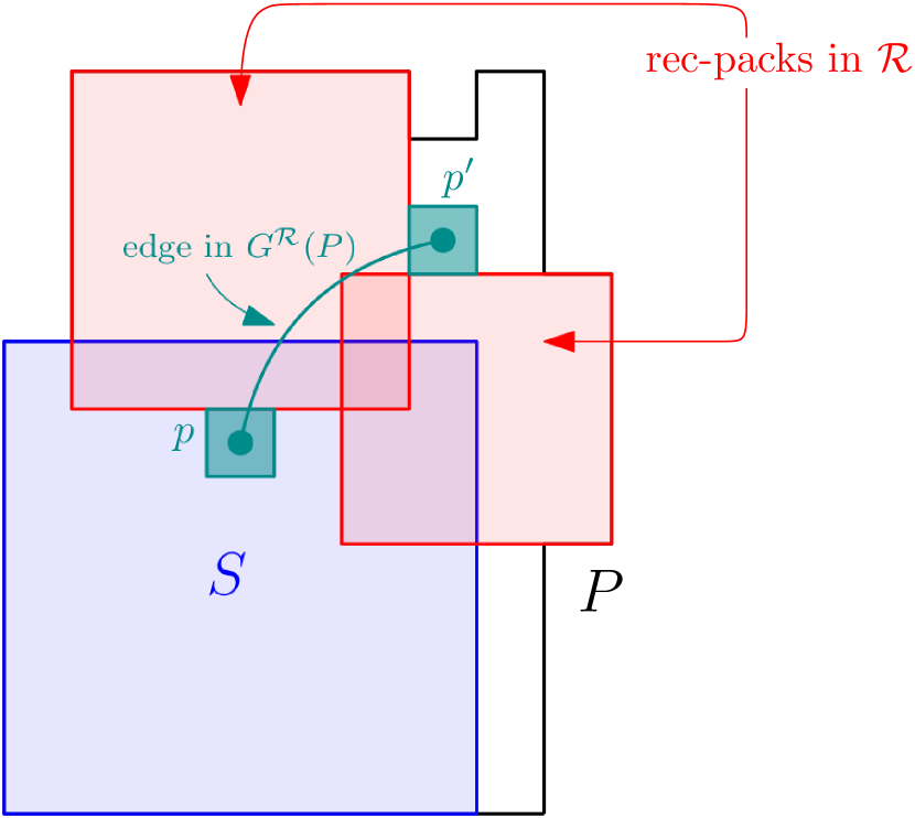
(a) Case I in proof of Lemma 3.16

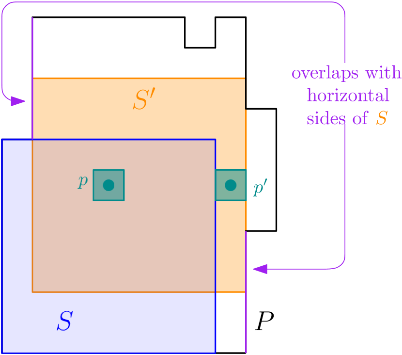
(b) Case II in proof of Lemma 3.16

Figure 7: Cases in proof of Lemma 3.16

Case II: $p$ and $p^{\prime}$ have the same $y$-coordinate.

Without loss of generality, let $p^{\prime}$ have a larger $x$-coordinate than $p$. Let $S^{\prime}$ be a maximal square covering both $p$ and $p^{\prime}$. If $S^{\prime}$ has its horizontal sides overlapping with polygon edges, we have an identical argument as before to prove that there is another maximal square $S^{\prime\prime}$ that covers $p$ and $p^{\prime}$ with a corner in $D_{y}$. Therefore, we only consider the case when $S^{\prime}$ has vertical sides that overlap with polygon edges (Figure 7(b)). Now, we move $S^{\prime}$ to the top until:

• it gets obstructed by a polygon edge to its top

• overlaps with some vertical polygon edge at just a point

• $p^{\prime}$ (and hence $p$) is on the bottom boundary of the square

Let the square obtained be $S_{t}$. In the first two cases, $S_{t}$ has a vertical edge overlapping with some vertical polygon edge (hence would have a corner in $D_{x}$, proving what we want). Therefore we only consider the third case: $p,p^{\prime}$ are on the bottom boundary of $S_{t}$. We similarly construct $S_{b}$ by moving $S^{\prime}$ to the bottom until either it gets obstructed by (i) a polygon edge to its bottom, (ii) overlaps with some vertical polygon edge at just a point, or (iii) $p^{\prime}$ (and hence $p$) is on the top boundary of the $S_{b}$. Again as the first two of these cases already achieve $S_{b}$ having a corner in $D_{x}$, we consider the third case: $p,p^{\prime}$ are on the top boundary of $S_{b}$. We observe that the bottom side of $S_{t}$ lies above or on the bottom side of $S$ (as $p,p^{\prime}$ are on the bottom boundary of $S_{t}$), and similarly the top side of $S_{b}$ lies below or on the top side of $S$. Again if $S_{t}$ has its bottom side lying on the bottom side of $S$, $S_{t}$ would have a corner in $D_{x}$ and we would be done; hence we consider that $S_{t}$ has its bottom side lying above the bottom side of $S$ (and $S_{b}$ has its top side lying below the top side of $S$). Further, the top side of $S_{t}$ must lie above or on the top side of $S$ (otherwise both the top side and the bottom edge of $S_{t}$ lie between the top side and bottom side of $S$; but $S_{t}$ covers $p^{\prime}$ which lies to the right of the right side of $S$; which means $S_{t}$ has its left side lying completely in the interior of $S$, contradicting that $S_{t}$ has vertical sides overlapping with polygon edges). However, this means if we were to vertically move a square initially positioned as $S_{t}$ (top side of $S_{t}$ above or on top side of $S$) to $S_{b}$ (top side of $S_{b}$ below top side of $S$), there would be a square $S_{1}$ with its top side lying on the top side of $S$ which contains $p$ and $p^{\prime}$. Moreover, as $S_{1}$ has its vertical sides overlapping with polygon edges (same polygon edges which were overlapping with the vertical sides of $S^{\prime}$, $S_{t}$ and $S_{b}$), $S_{1}$ has a corner in $D_{x}$.

Case II: $p$ and $p^{\prime}$ have the same $x$-coordinate.

An argument similar to the previous argument works.

This completes the proof.

3.3 Placing Rec-packs given a Partial Solution

We start with a result regarding placement of maximal squares to extend partial solutions.

Lemma 3.18.

Let $S$ be a maximal square of an orthogonal polygon $P$ with side length $d$ such that

• The top and bottom edges of $S$ overlaps with horizontal polygon edges $e_{1}$ and $e_{2}$ respectively.

• $e_{1}$ contains the top right corner of $S$ and the distance between the top right corner of $S$ and the right endpoint $e_{1}$ is more than $d$.

• $e_{2}$ contains the bottom right corner of $S$ and the distance between the bottom right corner of $S$ and the right endpoint of $e_{2}$ is more than $d$.

• There is a strip between $e_{1},e_{2}$, and the right side of the strip is more than $d$ distance away from the right side of $S$.

Let $S^{\prime}$ be the square generated by reflecting $S$ with respect to its right edge. Then, if there is a set of rec-packs $\mathcal{R}$ which is a partial solution of OPCS with $S\in\mathcal{R}$ and if $S^{\prime}$ does not overlap with any rec-pack in $\mathcal{R}$, then $\mathcal{R}\cup\{S^{\prime}\}$ is also a partial solution.

Proof 3.19.

Clearly $S^{\prime}$ is a valid square as it is bounded by the region in the polygon in between $e_{1}$ and $e_{2}$. Let $Y$ be strip the between $e_{1}$ and $e_{2}$.

Let $p$ be the block inside $S^{\prime}$ which is located at the top-left corner of $S^{\prime}$. Since $p$ is in the strip $Y$ defined by the region between $e_{1}$ and $e_{2}$, any valid square $S^{\prime\prime}$ covering $p$ must have side length at most $d$. Therefore, $S^{\prime\prime}$ must completely lie inside the union of the regions covered by $S$ and $S^{\prime}$.

Let $\mathcal{R}^{\prime}$ be a minimum cover of $P$ with $\mathcal{R}\subset\mathcal{R}^{\prime}$. Let $\mathcal{T}=\mathcal{R}^{\prime}\setminus\mathcal{R}$. Therefore $\mathcal{R}^{\prime\prime}=\mathcal{R}\cup\mathcal{E}(\mathcal{T})$ is also a minimum covering (as $\mathcal{E}(\mathcal{R}^{\prime\prime})=\mathcal{E}(\mathcal{R}^{\prime})=\mathcal{E}(\mathcal{R})\cup\mathcal{E}(\mathcal{T})$). Since $S^{\prime}$ does not overlap with any rec-pack in $\mathcal{R}$, there must be a square $S^{\prime\prime}\in\mathcal{E}(\mathcal{T})$ which covers $p$ (top-left block of $S^{\prime}$). However, $\{S,S^{\prime}\}$ covers a superset of the area that $\{S^{\prime\prime},S\}$ covers (as $S^{\prime\prime}$ has side length at most $d$). Therefore, we can remove $S^{\prime\prime}$ and add $S^{\prime}$ to $\mathcal{R}^{\prime\prime}$ (giving us $\mathcal{R}^{\prime\prime\prime}=(\mathcal{R}^{\prime}\setminus\{S^{\prime\prime}\})\cup\{S^{\prime}\}$) and this will still be a minimum cover. As $\mathcal{R}\cup\{S^{\prime}\}\subseteq\mathcal{R}^{\prime\prime\prime}$, $\mathcal{R}\cup\{S^{\prime}\}$ is a partial solution.

Remark 3.20.

This result symmetrically holds true for all four directions.

We can easily extend this result to placing a rec-pack to the right of the given square $S$.

Lemma 3.21.

Let $S$ be a maximal square of an orthogonal polygon $P$ with side length $d$ such that, for some natural number $\eta\in\mathbb{N}$,

• The top and bottom edges of $S$ overlaps with horizontal polygon edges $e_{1}$ and $e_{2}$ respectively.

• $e_{1}$ contains the top right corner of $S$ and the distance between the top right corner of $S$ and the right endpoint $e_{1}$ is more than $\eta d$.

• $e_{2}$ contains the bottom right corner of $S$ and the distance between the bottom right corner of $S$ and the right endpoint of $e_{2}$ is more than $\eta d$.

• There is a strip between $e_{1},e_{2}$, and the right side of the strip is more than $\eta d$ distance away from the right side of $S$.

Let $R$ be the rec-pack of width $d$ and strength $\eta$, such that the the vertical sides of $R$ are of length $d$ and the right side of the square $S$ coincides with the left side of $R$. Then, if there is a partial solution $\mathcal{R}$ of OPCS, where $S\in\mathcal{R}$ and $R$ does not overlap with any rec-pack in $\mathcal{R}$, then $\mathcal{R}\cup\{R\}$ is also a partial solution.

Proof 3.22.

We observe that $R$ lies completely inside the strip $Y$ in between $e_{1}$ and $e_{2}$. Further, we generate $\eta$ squares of the same size as $S$ as follows: $S_{1}$ is the square generated by reflecting $S$ by its right side, $S_{2}$ is the square generated by reflecting $S_{1}$ by its right side, and for any $i\in\{3,\ldots\eta\}$, $S_{i}$ is the square generated by reflecting $S_{i-1}$ by its right side. Therefore, $S_{\eta}$ is the square generated by reflecting $S_{\eta-1}$ by its right side. Then clearly, $R$ covers the exact area covered by $\{S_{1},\ldots,S_{\eta}\}$. Precisely, we have $\mathcal{E}(R)=\{S_{1},\ldots,S_{\eta}\}$. Moreover, as $R$ does not overlap with any rec-pack in $\mathcal{R}$, none of $\{S_{1},\ldots,S_{\eta}\}$ overlaps with any rec-pack in $\mathcal{R}$. This setting now allows us to use Lemma 3.18 repeatedly.

Since $S\in\mathcal{R}$, by Lemma 3.18, $\mathcal{R}\cup\{S_{1}\}$ is a partial solution. Again, as $\{S_{1}\}\in\mathcal{R}\cup\{S_{1}\}$, by Lemma 3.18, $\mathcal{R}\cup\{S_{1},S_{2}\}$ is a partial solution. Continuing, for any $i\in\{1,\ldots,\eta-1\}$, as $\mathcal{R}\cup\{S_{1},\ldots,S_{i}\}$ is a partial solution, by Lemma 3.21 $\mathcal{R}\cup\{S_{1},\ldots,S_{i},S_{i+1}\}$ is a partial solution. In particular, $\mathcal{R}\cup\{S_{1},\ldots,S_{\eta}\}=\mathcal{R}\cup\mathcal{E}(R)$ is a partial solution. This means $\mathcal{R}\cup R$ is also a partial solution.

Remark 3.23.

Again, this result symmetrically holds true for all four directions.

We will use Lemma 3.21 in the subsequent section to efficiently obtain a large number of squares which are also a part of a partial solution.

4 Polynomial Time Algorithm for OPCS w.r.t the Number of Polygonal Vertices

In this Section, we design an algorithm for OPCS such that the input polygon is taken in terms of its $n$ vertices. The algorithm runs in $\mathcal{O}(n^{14})$ time. We first start with some subroutines which we use for our algorithm, followed by the algorithm itself. Finally, we give the running time analysis for the algorithm.

4.1 Checking if a Set of Rec-Packs covers the Input Orthogonal Polygon

We design an algorithm that checks whether a given set of rec-packs completely covers an orthogonal polygon $P$.

Lemma 4.1.

Given an orthogonal polygon $P$ and a set $\mathcal{R}$ of $|\mathcal{R}|=D$ rec-packs, where $\mathcal{R}=\{R_{1},R_{2},\ldots,R_{D}\}$, there is an algorithm that checks if $\mathcal{R}$ (equivalently $\mathcal{E}(\mathcal{R})$) completely covers $P$. The algorithm runs in $\mathcal{O}(D\cdot(D+n)^{2})$ time.

Proof 4.2.

Clearly, if $\mathcal{R}$ does not completely cover the entire interior of $P$, the uncovered interior of $P$ will be a collection of one or more orthogonal polygons themselves. Further the edges of these polygons must be either an edge of $P$ or an edge of some rec-pack in $\mathcal{R}$. Therefore the vertices must be intersections of two such edges (either of $P$ or of some rec-pack in $\mathcal{R}$). Moreover, the number of such intersections is upper-bounded by $(2D+n)^{2}$. Therefore we check for each such intersection $\alpha$, if all four blocks with $\alpha$ as a corner are covered by some rec-pack in $\mathcal{R}$, then we are done.

Thus, the following algorithm answers whether $\mathcal{R}$ completely covers the orthogonal polygon $P$ in $\mathcal{O}(D\cdot(D+n)^{2})$ time.

Algorithm 1 Complete Coverage Checker     Input: Orthogonal Polygon $P$, $\mathcal{R}$

for all x-coordinates $x_{0}$ of vertical edges of $P$ and $\mathcal{R}$ do $\triangleright$ $\mathcal{O}(D+n)$ loop

     for all y-coordinates $y_{0}$ of horizontal edges of $P$ and $\mathcal{R}$ do $\triangleright$ $\mathcal{O}(D+n)$ loop

         for all four blocks $p$ with $(x_{0},y_{0})$ as corner do $\triangleright$ $\mathcal{O}(1)$ loop

              if $p$ lies outside $P$ then

                  continue to next iteration

              end if

              flag $\leftarrow$ FALSE $\triangleright$ To keep track if $s$ is covered

              for all $R\in\mathcal{R}$ do $\triangleright$ $\mathcal{O}(D)$ loop

                  if $p$ lies inside $R$ then $\triangleright$ $\mathcal{O}(1)$ check

                       flag $\leftarrow$ TRUE

                       break out from the current loop

                  end if

              end for

              if flag = FALSE then $\triangleright$ incomplete covering

                  return INCOMPLETE COVERING

              end if

         end for

     end for

end for

return COMPLETE COVERING

4.2 Detecting Unambiguous Squares

We now discuss an algorithm that takes in a square $S$, a partial solution $\mathcal{R}$ for OPCS and the input orthogonal polygon $P$ and decides if $S$ is an unambiguous square given $\mathcal{R}$. We crucially use Lemma 3.16 for the correctness of the algorithm.

Lemma 4.3.

Given an orthogonal polygon $P$, a partial solution $\mathcal{R}$ for OPCS and valid square $S$, there is an algorithm that checks if $S$ is an unambiguous square given $\mathcal{R}$ in $\mathcal{O}((n^{2}+|\mathcal{R}|n)^{3})$ time.

Proof 4.4.

We start by constructing the sets $D_{x}$ and $D_{y}$ as in Lemma 3.16. By definition, $|D_{x}|,|D_{y}|=\mathcal{O}((n+|\mathcal{R}|+1)\cdot n)=\mathcal{O}(n^{2}+|\mathcal{R}|n)$. Definition 3.10 implies that $S$ is an unambiguous square given $\mathcal{R}$ if and only if there is a simplicial node $p$ in $G^{\mathcal{R}}(P)$ such that $S$ covers $p$ and all its neighbours in $G^{\mathcal{R}}(P)$. From Lemma 3.16, this is not the case if and only if all maximal squares with a corner in $D_{x}\cup D_{y}$ which cover some block not covered by $\mathcal{R}\cup\{S\}$, together cover up the entire region inside $S$ not covered by $\mathcal{R}$. In other words, all blocks $p_{1}$ in $S$ not covered by $\mathcal{R}$ have an adjacent block $p_{2}$ in $G^{\mathcal{R}}(P)$ and therefore $p_{1}$ cannot be a simplicial node in $G^{\mathcal{R}}(P)$ with $S$ covering all its neighbours in $G^{\mathcal{R}}(P)$. Let $\mathcal{D}$ be the set of maximal squares with a corner in $D_{x}\cup D_{y}$ that cover some node in $G^{\mathcal{R}}(P)$ which is not covered by $S$ (i.e. we do not consider those maximal squares which lie completely outside the region covered by $\mathcal{R}\cup\{S\}$). By construction, $|\mathcal{D}|\leq 4|D_{x}|+4|D_{y}|=\mathcal{O}(n^{2}+|\mathcal{R}|n)$.

There is some block $p$ in $S$, which is not covered by any rec-pack in $\mathcal{D}\cup\mathcal{R}$, if and only if $p$ is a simplicial node in $G^{\mathcal{R}}(P)$ with $S$ covering $p$ and all its neighbours, i.e. $S$ is an unambiguous square given $\mathcal{R}$ (Lemma 3.16). However, we cannot check for simpliciality in all blocks in $S$, as this can potentially be exponential. Nevertheless, let us draw the infinite horizontal and vertical lines from all corners of rec-packs of $\mathcal{R}\cup\{S\}\cup\mathcal{D}$ and from the vertices of $P$. This would form a grid like structure with $\mathcal{O}((n^{2}+|\mathcal{R}|n)^{2})$ rectangular regions. Clearly, any two blocks in the same rectangular region would be covered by the same subset of rec-packs in $\mathcal{R}\cup\{S\}\cup\mathcal{D}$. Therefore it would be sufficient to check for simpliciality in a single block in each rectangular region (we check all the corner blocks of the rectangular regions i.e. blocks having a corner which shares an x coordinate of a vertex in $P$ or a corner in $\mathcal{R}\cup\{S\}\cup\mathcal{D}$ as well as the y coordinate). Given the description above, checking for simpliciality will take $\mathcal{O}(n^{2}+|\mathcal{R}|n)$ time.

Therefore, given $\mathcal{R}$ the following algorithm answers whether $S$ is an unambiguous square in $\mathcal{O}((n^{2}+|\mathcal{R}|n)^{3})$ time.

Algorithm 2 Is Unambiguous Square     Input: $P$, $\mathcal{R}$, $S$

If $S$ is not maximal return NOT UNAMBIGUOUS $\triangleright$ $\mathcal{O}(n)$ time

Construct $D_{x}$, $D_{y}$ as in Lemma 3.16 $\triangleright$ $|D_{x}|,|D_{y}|=\mathcal{O}(n^{2}+|\mathcal{R}|n)$

$\mathcal{D}^{\prime}\leftarrow$ {maximal squares with a corner in $D_{x}\cup D_{y}$} $\triangleright$ $\mathcal{O}((n^{2}+|\mathcal{R}|n)\cdot n)$ time

$\mathcal{D}\leftarrow$ {squares in $\mathcal{D}^{\prime}$ covering a block not covered by $\mathcal{R}\cup\{S\}$} $\triangleright$ $|\mathcal{D}|=\mathcal{O}(n^{2}+|\mathcal{R}|n)$

$T\leftarrow\{(x,y)|x\text{ and }y\text{ are coordinates of corners in }P\text{ or }\mathcal{R}\cup\mathcal{D}\cup\{S\}\}$

for $(x,y)\in T$ do $\triangleright$ $\mathcal{O}(|T|)=\mathcal{O}((|\mathcal{D}|+|\mathcal{R}|+n)^{2})=\mathcal{O}((n^{2}+|\mathcal{R}|n)^{2})$ loop

     for blocks $p$ with corner $(x,y)$ do $\triangleright$ at most $4$ possibilities

         if $p\in S$ and $\forall R\in\mathcal{R}\cup\mathcal{D},p\notin R$ then $\triangleright$ $\mathcal{O}(|\mathcal{D}|+|\mathcal{R}|)=\mathcal{O}(n^{2}+|\mathcal{R}|n)$ check

              return UNAMBIGUOUS $\triangleright$ $p$ is simplicial in $G^{\mathcal{R}}(P)$

         end if

     end for

end for

return NOT UNAMBIGUOUS

4.3 Generating Rec-Packs within a Strip

We wish to use Lemma 3.21 to extend an existing partial solution by adding a rec-pack. In order to do this, we need to construct rec-packs $R$ within a strip (between $e_{1}$, $e_{2}$, Lemma 3.21) which shares its shorter side (perpendicular to $e_{1}$ and $e_{2}$) with the side of a given square $S$ (we call this the ‘seed’). We discuss the following algorithm to construct rec-packs $R$ for the setting in Lemma 3.21.

Lemma 4.5.

Given a maximal square $S$ (referred to as the ‘seed’) of an orthogonal polygon $P$ with side length $d$, there is an algorithm to test if there are horizontal polygon edges $e_{1},e_{2}$ and some natural number $\eta\in\mathbb{N}$, such that

• The top and bottom edges of $S$ overlaps with horizontal polygon edges $e_{1}$ and $e_{2}$ respectively.

• $e_{1}$ contains the top right corner of $S$ and the distance between the top right corner of $S$ and the right endpoint $e_{1}$ is more than $\eta d$.

• $e_{2}$ contains the bottom right corner of $S$ and the distance between the bottom right corner of $S$ and the right endpoint of $e_{2}$ is more than $\eta d$.

• There is a strip between $e_{1},e_{2}$, and the right side of the strip is more than $\eta d$ distance away from the right side of $S$.

Moreover, if this exists, the algorithm finds the largest possible $\eta$ and if $\eta\geq 2$ the algorithm returns the rec-pack $R$ of width $d$ and strength $\eta-1$, such that the vertical sides of $R$ are of length $d$ and the right side of the square $S$ coincides with the left side of $R$. The algorithm runs in total $\mathcal{O}(n)$ time.

Note that this can be done for all four directions. Therefore, henceforth if we need to apply a similar algorithm in a different direction, we shall still refer to this Lemma.

This essentially tests if Lemma 3.21 can be applied to the setting or not; if yes, this also outputs the rec-pack $R$ with the second largest strength $\eta-1$ for which the setting applies.

Proof 4.6.

Consider the following algorithm.

Algorithm 3 Generate-Rec-pack-left     Input: $P$, seed $S$

Try finding $e_{1}$, $e_{2}$ containing top-left and bottom-right corner of $S$ $\triangleright$ $\mathcal{O}(n)$ check

if $e_{1}$ or $e_{2}$ not found then return NOT-APPLICABLE end if

$x_{1}\leftarrow$ x coordinate of right side of $S$

$x_{2}\leftarrow\min(\text{x coordinate of right end of }e_{1},\text{x coordinate of right end of }e_{2})$

$x_{2}\leftarrow\min(x_{2},\text{ x coordinate $x^{\prime}$ of polygon vertex lying between }e_{1},e_{2}:x^{\prime}>x_{1}$)

$d\leftarrow$ side length of $S$

if $x_{2}-x_{1}\leq d$ then return NOT-APPLICABLE end if $\triangleright$ Setting not applicable

$\eta\leftarrow\lceil\frac{x_{2}-x_{1}}{d}\rceil-1$ $\triangleright$ gets maximum possible strength $\eta$

if $\eta=1$ then return SHORT-STRIP end if

return rec-pack $R$ of strength $\eta$, width $d$ sharing left-side with right-side of $S$

This algorithm first checks for the existence of polygonal edges $e_{1}$ and $e_{2}$ ($\mathcal{O}(n)$ loop on all polygon-edge) and further checks if $e_{1}$ and $e_{2}$ have right end points lying farther than $\eta d$ distance for at least $\eta=1$ (the minimum value). If any of these do not happen, no such $R$ exists and the algorithm outputs ‘NOT-APPLICABLE’.

Moreover, if it is applicable, it finds the largest value of $\eta$ such that $e_{1},e_{2}$ have both of their right endpoints more than $\eta d$ distance away from the right side of $S$. Finally, the algorithm returns the rec-pack $R$ of strength $\eta-1$ as needed if $\eta\geq 2$ or returns ‘SHORT-STRIP’ if $\eta=1$.

The entire algorithm runs in linear time and can be extended to all directions.

The rec-packs generated in Algorithm 3 leaves at least distance $d$ and at most distance $2d$ from the right side of the strip contained in $e_{1}$, $e_{2}$ and can not intersect with any valid square that covers some region outside the strip containing $e_{1},e_{2}$.

The idea for generating $R$ with strength $\eta-1$ (or returning ‘SHORT-STRIP’ if $\eta=1$) is to ensure that $R$ does not intersect with any square that partially lies outside the strip in between $e_{1}$ and $e_{2}$. Moreover, if we get ‘SHORT-STRIP’ as an output, we know that there is no efficient rec-pack representation necessary as the number of squares needed to cover any such region with $\eta=1$ is at most $2$.

While using this as a subroutine for our final algorithm discussed later, we need to check that given a partial solution $\mathcal{R}\cup\{S\}$ with $S$ acting as a seed, if the generated rec-pack $R$ intersects with any rec-pack in $\mathcal{R}$. If there is no intersection, we can say that $\mathcal{R}\cup\{R\}$ is also a partial solution.

4.4 Polynomial Time Algorithm: Building up Partial Solutions

Finally, we are ready to state the polynomial time algorithm for OPCS when the input polygon is in terms of its $n$ vertices. We use the following framework: Start with an empty partial solution, keep extending the partial solution either by adding unambiguous squares (Lemma 3.12) or by adding rec-packs generated by a seed square (Algorithm 3 and Lemma 3.21). We stop this whenever we have a set of rec-packs which completely covers the polygon (detected using Algorithm 1). This will be guaranteed to be a minimum cover, because throughout the algorithm the set of rec-packs is guaranteed to be a partial solution by Lemma 3.12 and Lemma 3.21.

To find unambiguous squares given a partial solution $\mathcal{R}$ of OPCS, we generate all possible maximal squares having end points in $C_{x}\cup C_{y}$ as defined in Lemma 3.14. We are guaranteed to get an unambiguous square given $\mathcal{R}$ (due to Lemma 3.14). Next, we test for all such generated squares if it is unambiguous using Algorithm 2.

Formally, the algorithm is as follows.

Algorithm 4 Extend-Partial-Solution     Input: $P$

$\mathcal{R}\leftarrow\emptyset$ $\triangleright$ Start with empty partial solution

while $\mathcal{R}$ does not cover $P$ do $\triangleright$ $\mathcal{O}(|\mathcal{R}|\cdot(|\mathcal{R}|+n)^{2})$ time check with Algorithm 1

     Construct $C_{x},C_{y}$ as Lemma 3.14 $\triangleright$ $|C_{x}|,|C_{y}|=\mathcal{O}(n\cdot(n+|\mathcal{R}|))$

     $\mathcal{S}^{\prime}\leftarrow\{\text{squares with corner in }C_{x}\cup C_{y}\}$ $\triangleright$ $|\mathcal{S}^{\prime}|=\mathcal{O}(n\cdot(n+|\mathcal{R}|))$, time $=\mathcal{O}(|\mathcal{S}^{\prime}|\cdot n)$

     for $S\in\mathcal{S}^{\prime}$ do $\triangleright$ $|\mathcal{S}^{\prime}|=\mathcal{O}(n\cdot(n+|\mathcal{R}|))$ loop

         if $S$ is unambiguous in $P$ given $\mathcal{R}$ then$\triangleright$ $\mathcal{O}((n^{2}+|\mathcal{R}|n)^{3})$ using Algorithm 2

              $\mathcal{R}\leftarrow\mathcal{R}\cup\{S\}$ $\triangleright$ $\mathcal{R}$ is still a partial solution by Lemma 3.12

              $R_{l}\leftarrow$ generated rec-pack with seed $S$ to the left. $\triangleright$ $\mathcal{O}(n)$ with Algorithm 3

              $R_{r}\leftarrow$ generated rec-pack with seed $S$ to the right. $\triangleright$ Similar to Algorithm 3

              $R_{t}\leftarrow$ generated rec-pack with seed $S$ to the top. $\triangleright$ Similar to Algorithm 3

              $R_{b}\leftarrow$ generated rec-pack with seed $S$ to the bottom. $\triangleright$ Similar to Algorithm 3

              for $R\in\{R_{l},R_{r},R_{t},R_{b}\}$ do $\triangleright$ $\mathcal{O}(1)$ loop

                  if $R\notin$ {NOT-APPLICABLE, SHORT-STRIP} then $\triangleright$ Algorithm 3 output

                       if $R$ does not intersects with any rec-pack in $\mathcal{R}$ then $\triangleright$ $\mathcal{O}(n)$ check

                           $\mathcal{R}\leftarrow\mathcal{R}\cup\{R\}$ $\triangleright$ $\mathcal{R}$ remains a partial solution by Lemma 3.21

                       end if

                  end if

              end for

              break out of for loop, continue next while loop iteration

         end if

     end for

end while

$s\leftarrow 0$

for $R\in\mathcal{R}$ do $\triangleright$ $\mathcal{O}(|\mathcal{R}|)$ loop

     $s\leftarrow s+(\text{strength of }R)$ $\triangleright$ $|\mathcal{E}(R)|=$ strength of $R$.

end for

return $s$

First, as the generated rec-packs are only added to $\mathcal{R}$ if they do not intersect with any rec-pack in $\mathcal{R}$, we make the following observation.

The only non-trivial rec-packs in $\mathcal{R}$ are the ones generated by a seed, and no two non-trivial rec-packs in $\mathcal{R}$ intersect with each other.

From the discussion above, we obtain the following statement.

Lemma 4.7.

Algorithm 1 (Extend-Partial-Solution) terminates in finite time and outputs the minimum number of squares to cover $P$.

Proof 4.8.

Termination. Each iteration of the while loop takes finite time and every other step outside the while loop takes finite time as well. Moreover, the number of while loop iterations is also finite as at each step, as in each step the algorithm is guaranteed to find an unambiguous square (Lemma 3.14) and therefore the size of the partial solution increases at least by one. Further, this unambiguous square added covers at least one currently uncovered block of the polygon, thereby decreasing in the current step the area of the uncovered region of the polygon at least by $1$. Since $P$ has a finite area, the number of while loop iterations is finite, and hence Algorithm 4 terminates in finite time.

Minimum Covering. By Lemma 3.12 and Lemma 3.21, $\mathcal{R}$ is always a partial solution, and therefore if $\mathcal{R}$ covers $P$ completely, it has to be a minimum cover. This means $\mathcal{E}(\mathcal{R})$ is a minimum cover. Therefore, we have,

$$\text{{OPCS}}(P)=|\mathcal{E}(\mathcal{R})|=|\bigcup\limits_{R\in\mathcal{R}}\mathcal{E}(R)|=\sum\limits_{R\in\mathcal{R}}|\mathcal{E}(R)|=\sum\limits_{R\in\mathcal{R}}(\text{strength of }R)$$

which completes the proof.

Our next step is to bound the time for each iteration of the while loop.

Lemma 4.9.

Each iteration of the while loop of Algorithm 4 runs in $\mathcal{O}((n^{2}+|\mathcal{R}|n)^{4})$ time.

Proof 4.10.

We analyse the time taken at each step.

• Checking the condition of the while loop takes $\mathcal{O}(|\mathcal{R}|\cdot(|\mathcal{R}|+n)^{2})$ time, which is clearly bounded by $\mathcal{O}((n^{2}+|\mathcal{R}|n)^{4})$.

• Generating $\mathcal{S}^{\prime}$, and checking for all possible squares in $\mathcal{S}^{\prime}$ if they are ambiguous takes time $\mathcal{O}((n^{2}+|\mathcal{R}|n)\cdot n+(n^{2}+|\mathcal{R}|n)\cdot(n^{2}+|\mathcal{R}|n)^{3})=\mathcal{O}((n^{2}+|\mathcal{R}|n)^{4})$ as $|S^{\prime}|=\mathcal{O}(n^{2}+|\mathcal{R}|n)$

• Generating rec-packs with the seed $S$ and the respective checks are only done four times per while loop iteration, and therefore they take up a total overhead of $\mathcal{O}(n)$.

Hence, each iteration of the while loop in Algorithm 4 takes $\mathcal{O}((n^{2}+|\mathcal{R}|n)^{4})$ time.

We now bound the total time in terms of the size of final set of rec-packs $\mathcal{R}$.

Lemma 4.11.

If the final set of rec-packs from Algorithm 4 is $\mathcal{R}$, then the running time is $\mathcal{O}(|\mathcal{R}|\cdot(n^{2}+|\mathcal{R}|n)^{4}))$.

Proof 4.12.

By Lemma 4.9, we know that each while loop iteration takes at most $\mathcal{O}((n^{2}+|\mathcal{R}|n)^{4})$ time. As the size of $\mathcal{R}$ increases at least by one at each iteration, the number of while loop iterations must be bounded by $|\mathcal{R}|$, the size of the final rec-pack minimum cover. Therefore, the total time for all while loop iterations is $\mathcal{O}(|\mathcal{R}|\cdot(n^{2}+|\mathcal{R}|n)^{4}))$. As there is only a total overhead of $\mathcal{O}(|\mathcal{R}|)$ outside the while loop, the total running time of Algorithm 4 becomes $\mathcal{O}(|\mathcal{R}|\cdot(n^{2}+|\mathcal{R}|n)^{4}))$.

Remark 4.13.

If we only extended our partial solutions by unambiguous squares (and not generate rec-packs from a seed), we would finally have a set of trivial rec-packs (squares) $\mathcal{S}$ which is a minimum cover of $P$ with OPCS $(P)=|\mathcal{S}|$. This would give us an output sensitive algorithm of $\mathcal{O}(|\mathcal{S}|\cdot(n^{2}+|\mathcal{S}|n)^{4}))$

We now proceed to bound the size of the final set $\mathcal{R}$ of rec-packs in Algorithm 4.

Lemma 4.14.

If $\mathcal{R}$ be the final set of rec-packs in Algorithm 4, then $|\mathcal{R}|=\mathcal{O}(n^{2})$

Proof 4.15.

Let $\mathcal{R}_{g}\subseteq\mathcal{R}$ be the set of rec-packs generated from a seed, and let $\mathcal{R}_{u}\subseteq\mathcal{R}$ be the set of unambiguous squares appearing as trivial rec-packs in $R$. Therefore, $\mathcal{R}=\mathcal{R}_{g}\cup\mathcal{R}_{u}$.

Claim 1.

For any set of squares $\mathcal{S}$ such that $\mathcal{E}(\mathcal{R}_{g})\cup\mathcal{S}$ covers $P$, we must have $|\mathcal{S}|\geq|\mathcal{R}_{u}|$.

Proof 4.16.

Since $\mathcal{R}$ is a minimum cover (Lemma 4.7), $\mathcal{E}(\mathcal{R})=\mathcal{E}(\mathcal{R}_{g})\cup\mathcal{R}_{u}$ is a minimum cardinality set of squares covering $P$. Therefore, for any set of squares $\mathcal{S}^{\prime}$ that covers $P$, we must have $|\mathcal{S}^{\prime}|\geq|\mathcal{E}(\mathcal{R}_{g})\cup\mathcal{R}_{u}|$. In particular, for any set of squares $\mathcal{S}$ such that $\mathcal{E}(\mathcal{R}_{g})\cup\mathcal{S}$ covers $P$, we must have $|\mathcal{E}(\mathcal{R}_{g})\cup\mathcal{S}|\geq|\mathcal{E}(\mathcal{R}_{g})\cup\mathcal{R}_{u}|$. This means that $|\mathcal{S}|\geq|\mathcal{R}_{u}|$ (as $\mathcal{R}_{u}$ and $\mathcal{E}(\mathcal{R}_{g})$ are disjoint).

We now construct such a set of squares $\mathcal{S}$ of size $\mathcal{O}(n^{2})$. Let us draw a vertical line and a horizontal line through each vertex $v$ of $P$. Let us call them vertex induced lines of $P$. As $P$ has $n$ vertices, there are at most $n$ vertex induced vertical lines and $n$ vertex induced horizontal lines.

These vertex induced lines form a grid like structure resulting in rectangular grid cells formed between two consecutive vertex induced vertical lines and two consecutive vertex induced horizontal lines. Let $abcd$ be a such a rectangular grid cell formed by consecutive vertex induced vertical & horizontal lines, that lies in the interior (possibly overlapping with some of the polygon edges of $P$), as shown in Figure 8. Let $a$ be the top-left corner, $b$ be the top-right corner, $c$ be the bottom-right corner and $d$ be the bottom left corner. Without loss of generality, let the rectangle $abcd$ have its vertical sides no longer than the horizontal sides (i.e. length is along the $x$-axis). We now present a method to cover the entire rectangular region $abcd$ (possibly covering some more portion of the interior of the polygon) with at most $5$ more valid squares (if we consider $\mathcal{R}_{g}$ to be already placed).

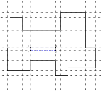
Figure 8: Defining the rectangular region $abcd$

Consider the two consecutive vertex induced vertical lines $l_{1},l_{2}$, one passing through $a,d$ and the other passing through $b,c$. There cannot be any vertex $v$ of $P$ lying strictly between these two lines (otherwise, these would not be adjacent vertex induced lines). As $abcd$ lies inside $P$, the following must hold (Figure 9(a)):

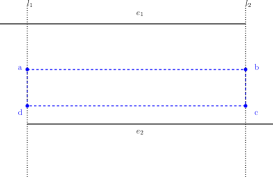
(a) The edges $e_{1},e_{2}$

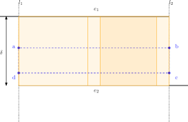
(b) Covering of $abcd$

Figure 9: $3$ more squares cover $abcd$

• There must be a horizontal polygon edge $e_{1}$ of $P$ that intersects both $l_{1}$ and $l_{2}$ (possibly at its endpoint), and that either overlaps with the line segment $ab$ or lies above $ab$.

• There must be a horizontal polygon edge $e_{2}$ of $P$ that intersects both $l_{1}$ and $l_{2}$ (possibly at its endpoint), and that either overlaps with the line segment $cd$ or lies under $cd$.

• The rectangular region enclosed by $e_{1}$, $e_{2}$, $l_{1}$, $l_{2}$ entirely lies inside the polygon $P$.

Let $\delta$ denote the vertical distance between $e_{1}$ and $e_{2}$. Further, if $\overline{e_{i}}$ is the length of an edge $e_{i}$, then $\overline{e_{1}},\overline{e_{2}}\geq\overline{ab}$ ($e_{1}$, $e_{2}$ intersect both $l_{1}$, $l_{2}$). We now discuss the following cases.

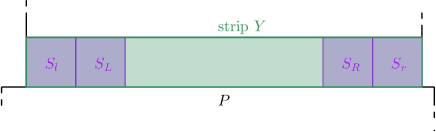
Figure 10: Defining $S_{l},S_{r},S_{L},S_{R}$ in the strip $Y$

• Case I: $5\delta\geq\overline{ab}$. In this case, we can draw at most three $\delta\times\delta$ squares which cover the entire rectangular region enclosed by $e_{1}$, $e_{2}$, $l_{1}$, $l_{2}$ and hence covers $abcd$ (Figure 9(b)). Therefore $abcd$ can be covered by at most $3$ squares.

• Case II: $5\delta<\overline{ab}$. In this case, there must be a (unique) strip $Y$ that is enclosed within $e_{1}$, $e_{2}$ (Section 2). $Y$ must have an aspect ratio of more than $5$. Let $S_{0}\in\mathcal{R}$ be the first $\delta\times\delta$ square placed that covers some portion in $Y$ when Algorithm 4 is run on $P$ (there would always be a $\delta\times\delta$ square placed in $Y$ as no square with smaller dimension can generate a rec-pack as a seed that overlaps with $Y$, and all maximal squares covering any block which is at a distance of more than $\delta$ from the left & right boundary of $Y$, have dimension $\delta\times\delta$). Let $S_{l}$ be the left most $\delta\times\delta$ square lying inside $Y$ and $S_{L}$ be the square obtained by reflecting $S_{l}$ about its right side. Similarly, let $S_{r}$ be the right most $\delta\times\delta$ square lying inside $Y$ and $S_{R}$ be the square obtained by reflecting $S_{r}$ about its left side (Figure 10). Since the aspect ratio of $Y$ is more than $5$, $S_{l}$,$S_{L}$,$S_{R}$,$S_{r}$ are pairwise non-overlapping $\delta\times\delta$ squares that inside Y. Moreover since $Y$ is a strip with $\delta$ as the length of the shorter side, there cannot be a valid square that covers some region outside $Y$ as well as some region inside $Y$ which is not covered by $S_{l}$,$S_{r}$. Consider the portion $Y_{l}$ of $Y$ lying to the left hand side of $S_{0}$. Either $Y_{l}$ is entirely covered by $S_{l}$ and $S_{L}$, or the horizontal distance between the left side of $S_{0}$ and the left side of $Y_{l}$ is more than $2\delta$. Even if the second case occurs, then Algorithm 1 must generate $R_{l}\in\mathcal{R}_{g}$ as the rec-pack lying to the left of the seed $S_{0}$ which intersects with $S_{L}$ (as $S_{0}$ is the first square placed in the strip $Y$ and hence generates a rec-pack $R_{l}$ with the left side at most $2\delta$ distance from the left side of $Y$, and hence $R_{l}$ cannot intersect with any square or re-pack in the partial solution found before $S_{0}$ was added, Section 4.3). This means $Y_{l}$ is entirely covered by $S_{l}$, $S_{L}$ and possibly some rec-pack in $\mathcal{R}_{g}$. Similarly, the portion $Y_{r}$ of $Y$ to the right of $S$ is entirely covered by $S_{r}$, $S_{R}$ and possibly some rec-pack in $\mathcal{R}_{g}$. Therefore the entire region of $Y$ (and hence $abcd$) is covered by $\mathcal{R}_{g}$ and $5$ more squares, $\{S_{0},S_{l},S_{L},S_{R},S_{r}\}$.

If we repeat the same process for each rectangular region $abcd$ formed by consecutive vertex induced lines, then we can cover up the entire polygon $P$ using just $5$ more squares for each such rectangular region lying inside $P$ (along with the rec-packs in $R_{g}$). However, the total number of such rectangular region is $\mathcal{O}(n^{2})$. Therefore, if $\mathcal{S}$ is the set of all such squares (at most $5$ of them per rectangular region $abcd$), then $|\mathcal{S}|=\mathcal{O}(n^{2})$ and $\mathcal{E}(\mathcal{R}_{g})\cup S$ is a set of squares covering the entire polygon $P$. As discussed in 1, we have $|\mathcal{R}_{u}|\leq|\mathcal{S}|=\mathcal{O}(n^{2})$.

Moreover, as for each unambiguous square $S$, Algorithm 4 adds at most four rec-packs with seed $S$, the number of rec-packs generated from a seed can be at most $4$ times the number of unambiguous squares. Therefore $|\mathcal{R}_{g}|\leq 4|\mathcal{R}_{u}|=\mathcal{O}(n^{2})$.

Hence, $|\mathcal{R}|=|\mathcal{R}_{g}|+|\mathcal{R}_{u}|=\mathcal{O}(n^{2})$.

This allows us to derive the algorithmic running time purely in terms of $n$.

Theorem 4.17.

For an orthogonal polygon $P$ with $n$ vertices, Algorithm 4 outputs $\textsc{OPCS}(P)$ in $\mathcal{O}(n^{14})$ time.

Proof 4.18.

The correctness of the algorithm is due to Lemma 4.7. For the analysis of the running time of Algorithm 4, we substitute the bound of $|\mathcal{R}|=\mathcal{O}(n^{2})$ obtained in Lemma 4.14 in the time complexity of Lemma 4.11. Therefore,

Running time of Algorithm 4 $$=\mathcal{O}(|\mathcal{R}|\cdot(n^{2}+|\mathcal{R}|n)^{4})) [\text{\lx@cref{creftype~refnum}{lem:time-square-count}}]$$

$$=\mathcal{O}(n^{2}\cdot(n^{2}+n^{2}\cdot n)^{4})) [|\mathcal{R}|=\mathcal{O}(n^{2}),\text{\lx@cref{creftype~refnum}{lem:R-bound}}]$$

$$=\mathcal{O}(n^{2}\cdot(n^{3})^{4})=\mathcal{O}(n^{14})$$

This completes the proof.

Remark 4.19.

To report the solution instead of just the count, we could return the set $\mathcal{R}$ of rec-packs in Algorithm 4. Here, rec-packs are used to efficiently encode multiple squares (potentially exponentially many) into constant sized information.

Remark 4.20.

Here we assumed that arithmetic operations take constant time. However, even if each arithmetic operation took polynomial time, the total runtime would still be polynomial as there are only polynomially many arithmetic operations done.

5 Improved Algorithm for Orthogonal Polygons with $k$ Knobs

In this section, we design an algorithm for $p$-OPCS where along with the number $n$ of vertices of the input orthogonal polygon we also have the parameter $k$, which is the number of knobs (Definition 2.4) in $P$. This algorithm works better than Algorithm 4 when are input instances are such that $k=o(n^{13/14})$.

First, we define a special structure called separating squares and crucially use it to construct our recursive algorithm. We solve the base cases of the recursive algorithm using Algorithm 4.

5.1 More on Structure of Minimum Covering

We define our crucial structure of a separating maximal corner square (or simply, a separating square) and use the definition to further explore properties of non-knob convex vertices (Definition 2.5).

Definition 5.1 (Separating Maximal Corner Square).

Let $P$ be an orthogonal polygon. For a convex vertex $v$, $MCS(v)$ is said to be a separating maximal corner square or simply a separating square if the region inside $P$ but not inside $MCS(v)$ is not a connected region (Figure 11).

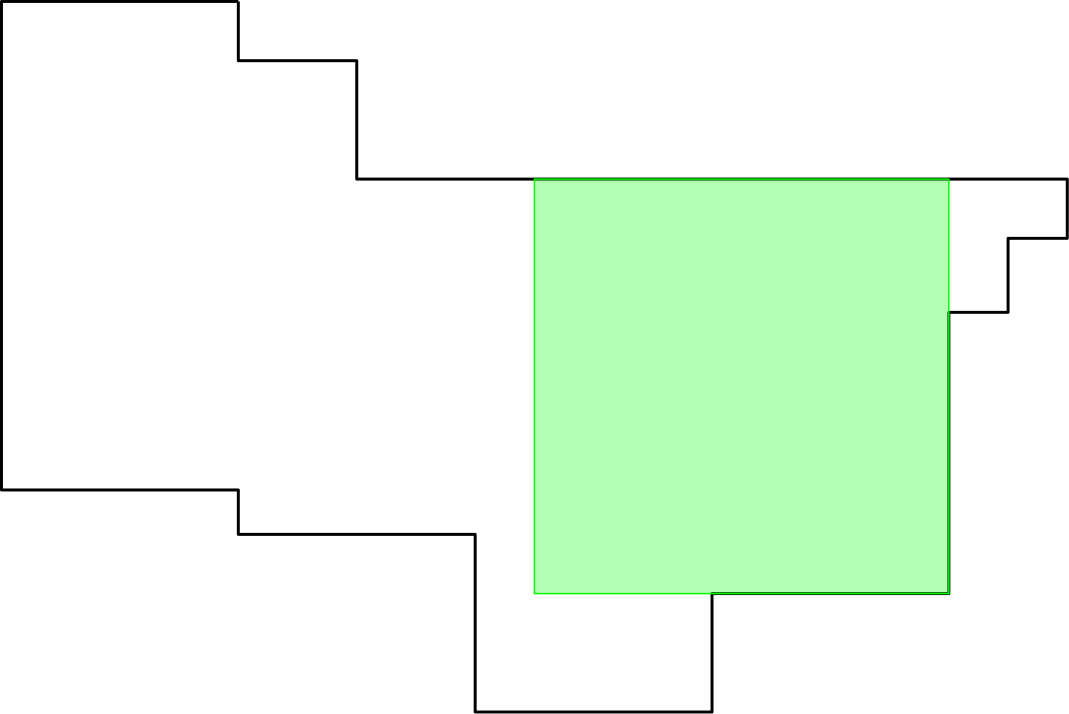
(a) A separating square

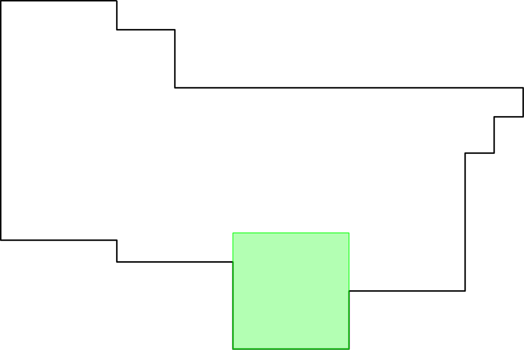
(b) A maximal square which is not a separating square

Figure 11: Separating Maximal Corner Square

This gives us the following result.

Lemma 5.2.

If $v_{i}$ is a non-knob convex vertex (Definition 2.5) of an orthogonal polygon $P$, then $MCS(v_{i})$ is a separating square which separates $v_{i-2}$ and $v_{i+2}$.

Proof 5.3.

If $v_{i}$ is a non-knob convex vertex, then any curve lying in $P$ and having end points at $v_{i+2}$ and $v_{i-2}$ must intersect $MCS(v_{i})$ and hence $MCS(v_{i})$ must be a separating square separating $v_{i-2}$ and $v_{i+2}$.

Remark 5.4.

Given an orthogonal polygon $P$, we can find a non-knob convex vertex in $\mathcal{O}(n)$ time (if it exists) by a simple check on all vertices (or report no non-knob convex vertex exist).

We now use this to recursively obtain simpler instances from an input instance $P$.

5.2 Recursion with Separating Squares

Recall that a separating square separates an input orthogonal polygon $P$ into unconnected uncovered regions. We will construct two polygons from these uncovered polygons which still preserves the information about $\textsc{OPCS}(P)$. First, we need the following terminology.

Definition 5.5.

Given an orthogonal polygon $P$, let $S$ be a (maximal) separating square which is a maximal square due to a non-knob convex vertex of $P$. We classify the set of connected components of $P$ that are separated by $S$ as follows,

• $Q_{t}$ be the connected components separated by $S$ that only intersect at more than one point with the top side of $S$ (and no other side).

• $Q_{b}$ be the connected components separated by $S$ that only intersect at more than one point with the bottom side of $S$ (and no other side).

• $Q_{l}$ be the connected components separated by $S$ that only intersect at more than one point with the left side of $S$ (and no other side).

• $Q_{r}$ be the connected components separated by $S$ that only intersect at more than one point with the right side of $S$ (and no other side).

• $Q_{tr}$ be the connected components separated by $S$ that only intersect at more than one point with the top side and right side of $S$ and also at the top-right corner of $S$.

• $Q_{br}$ be the connected components separated by $S$ that only intersect at more than one point with the bottom side and right side of $S$ and also at the bottom-right corner of $S$.

• $Q_{tl}$ be the connected components separated by $S$ that only intersect at more than one point with the top side and left side of $S$ and also at the top-left corner of $S$.

• $Q_{bl}$ be the connected components separated by $S$ that only intersect at more than one point with the left side and right side of $S$ and also at the bottom-left corner of $S$.

• $Q_{trb}$ be the connected components separated by $S$ that only intersect at more than one point with the top side, bottom side and right side of $S$ and also at the top-right corner and the bottom-right corner of $S$.

• $Q_{tlb}$ be the connected components separated by $S$ that only intersect at more than one point with the top side, bottom side and left side of $S$ and also at the top-left corner and the bottom-left corner of $S$.

• $Q_{rbl}$ be the connected components separated by $S$ that only intersect at more than one point with the right side, bottom side and left side of $S$ and also at the bottom-right corner and the bottom-left corner of $S$.

• $Q_{rtl}$ be the connected components separated by $S$ that only intersect at more than one point with the right side, top side and left side of $S$ and also at the top-right corner and the top-left corner of $S$.

Let $\mathcal{Q}^{\prime}=\{Q_{t},Q_{b},Q_{r},Q_{l},Q_{tr},Q_{br},Q_{tl},Q_{bl},Q_{trb},Q_{tlb},Q_{rbl},Q_{rtl}\}$ and let $\mathcal{Q}=\{Q\in\mathcal{Q}^{\prime}|Q\text{ is nonempty}\}$.

Lemma 5.6.

Given an orthogonal polygon $P$, let $S$ be a (maximal) separating square which is a maximal square due to a non-knob convex vertex of $P$ and $\mathcal{Q}$ be as defined in 5.5. Then the following must hold true.

• $\forall Q\in\mathcal{Q}$, $S\cup Q$ is a connected orthogonal polygon without holes.

• $\text{{OPCS}}(P)=\big{(}\sum\limits_{Q\in\mathcal{Q}}\text{{OPCS}}(S\cup Q)\big{)}-(|\mathcal{Q}|-1)$

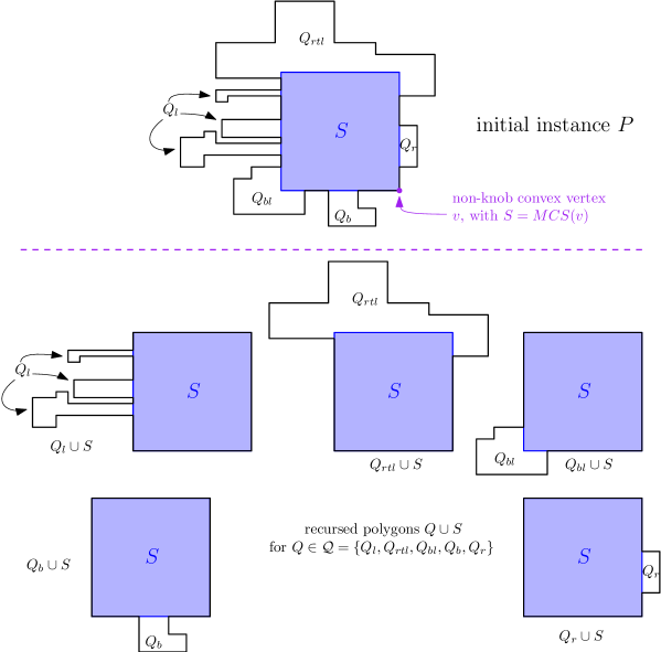
Figure 12: $\text{{OPCS}}(P)=\big{(}\sum\limits_{Q\in\mathcal{Q}}\text{{OPCS}}(S\cup Q)\big{)}-(|\mathcal{Q}|-1)$ with $\mathcal{Q}=\{Q_{l},Q_{rtl},Q_{r},Q_{bl},Q_{b}\}$ in this case

Proof 5.7.

First, we observe that since $S$ is a separating square which is a maximal square due to a non-knob convex vertex $v$, there cannot be a component that intersects with three vertices of $S$ (otherwise $S$ would not be maximal and could be grown by fixing a corner at $v$).

To see that for all $Q\in\mathcal{Q}$, $S\cup Q$ is connected, it is sufficient to observe that we can find a curve in the strict interior of $S\cup Q$ from any point $t_{1}$ in its interior to any point $t_{2}$ in its interior; either lying inside a single connected component of $Q$ (if $t_{1},t_{2}$ are in that component), or through $S$ (if $t_{1},t_{2}$ are in different components of $Q$). Further, $Q\cup S$ cannot have holes as $P$ does not have holes.

Moreover, we observe that there cannot be a valid square of $P$ that covers two different points from distinct $Q,Q^{\prime}\in\mathcal{Q}$ (this would contradict the maximality of $S$). Also, in a minimum covering with $S$ as one of the squares, all other valid squares must cover at least one point from the interior of exactly one $Q\in\mathcal{Q}$ (otherwise this square would be completely inside $S$, hence redundant). Therefore if $P$ is covered using a set $\mathcal{S}$ of $C$ squares including $S$, we can cover $Q\cup S$ using the squares in $\mathcal{S}$ that cover some part of $Q$ and the square $S$ itself. If we do this for all $Q\in\mathcal{Q}$ this uses $C+(|\mathcal{Q}|-1)$ squares as $S$ is in this cover of all $|\mathcal{Q}|$ instances $Q\cup S$, but appear only once in $\mathcal{S}$ (other squares in $\mathcal{S}$ appear exactly once in a cover of $Q\cup S$ for exactly one $Q\in\mathcal{Q}$). Since we start with a minimum cover of $P$ and find a valid cover of all $Q\cup S$ polygons with exactly $(|\mathcal{Q}|-1)$ more squares in total, we get,

$$\text{{OPCS}}(P)\geq\big{(}\sum\limits_{Q\in\mathcal{Q}}\text{{OPCS}}(S\cup Q)\big{)}-(|\mathcal{Q}|-1)$$

Given any minimum covering of all $Q\cup S$, all such instances must contain $S$ (as $S$ is a maximum corner square in both). So we superimpose these coverings and delete all but one $S$ to get a covering of $P$. This time we started from a minimal covering of the individual $Q\cup S$ polygons to get a valid covering of $P$. Including this with the rest of the result, we obtain

$$\text{{OPCS}}(P)=\big{(}\sum\limits_{Q\in\mathcal{Q}}\text{{OPCS}}(S\cup Q)\big{)}-(|\mathcal{Q}|-1)$$

Remark 5.8.

$|\mathcal{Q}|\leq|\mathcal{Q}^{\prime}|=12$ in Lemma 5.6. Moreover, there are combinations (like $Q_{tr}$ and $Q_{trb}$) that cannot both be non-empty in $P$.

We now prove a crucial result that such a recursive step does not increase the number of knobs in each individual instance $Q\cup S$.

Lemma 5.9.

Let $S$ be a (maximal) separating square which is a maximal square due to a non-knob convex vertex of an orthogonal polygon $P$ with $n$ vertices and $k$ knobs. Let $\mathcal{Q}$ be defined as in Definition 5.5. Then, $\forall Q\in\mathcal{Q},(Q\cup S)$ is an orthogonal polygon without holes with at most $n$ vertices and at most $k$ knobs. Moreover, any vertex in $Q\cup S$ which is a corner of $S$ is part of a knob in $Q\cup S$ along a side of $S$.

Proof 5.10.

Lemma 5.6 already proves that $\forall Q\in\mathcal{Q},(Q\cup S)$ is an orthogonal polygon without holes. Further, the number of vertices can only decrease because the only time a new vertex (vertex not in $P$) would be introduced is when $S$ already distributes the existing vertices of $P$ in each of $(Q\cup S),Q\in\mathcal{Q}$ (causing no total increase in the number of vertices in $(Q\cup S)$ than in $P$). We now prove that $\forall Q\in\mathcal{Q},Q\cup P$ has at most $k$ knobs.

Consider $Q\cup S$ for some $Q\in\mathcal{Q}$. Without loss of generality assume $Q$ is either $Q_{l}$ or $Q_{tl}$ or $Q{tlb}$ (all other cases have symmetric arguments). We now show that for all knobs in $Q\cup S$, there is a distinct knob in $P$ (which would show that $Q\cup S$ has at most $k$ knobs if $P$ has at most $k$ knobs. Clearly any (distinct) knob $(u1,u2)$ of $Q\cup S$ such that $u1$, $u_{2}$ are not corners in $S$, $(u_{1},u_{2})$ must be a (distinct) knob in $P$ (knob in $Q$, in particular). Hence we only need to consider knobs which $(u_{1},u_{2})$ in $Q\cup S$ such that either $u_{1}$ or $u_{2}$ is a vertex of $S$. Without loss of generality, we assume that $u_{1}$ is a corner in $S$.

• Case I: $Q=Q_{tlb}$. In this case the top-left and the bottom-left corners of $S$ completely lie inside $Q$ and hence are not vertices of $Q\cup S$. Therefore $u_{1}$ is either the bottom-right corner or the top-right corner of $S$ (both are vertices in $Q\cup S$). Without loss of generality, assume $u_{1}$ to be the top-right corner of $S$. Consider $e_{1}$ to be the horizontal edge of $Q\cup S$ (i.e. the edge overlapping with top edge of $S$) with $u_{1}$ as a corner. Since $Q_{tlb}$ intersects with the right corner of $S$, $e_{1}$ has to shorter than the side length of $S$. As the entire region inside $S$ is inside $Q\cup S$, the other end point of $e_{1}$ must be a concave vertex. Therefore $(u_{1},u_{2})\neq e_{1}$. Moreover, as the other end point of the vertical edge of $Q\cup S$ from $u_{1}$ is the bottom-right corner of $S$, $u_{2}$ must be the bottom right corner of $S$; $(u_{1},u_{2})$ must be a left knob (and the only knob) in $Q\cup S$ (which proves that all vertices in $Q\cup S$ which are corners in $S$ are part of knobs in $Q\cup S$, along a side of $S$). Moreover, for this knob $(u_{1},u_{2})$, can find a left knob of the region $P\setminus Q$ (which must be a knob in $P$ as $P\setminus Q$ intersects $Q$ only in top, bottom and right edges). Therefore, in this case, for every knob in $S\cup Q$, we can find a distinct knob in $P$.

• Case II: $Q=Q_{tl}$. We consider four subcases.

  • Case II(a): $Q$ does not touch the top-right corner or the bottom-left corner of $S$. By arguments similar to above, we can show that right side of $S$ and the bottom side of $S$ are right and bottom knobs of $Q\cup S$ (which proves that all vertices in $Q\cup S$ which are corners in $S$ are part of knobs in $Q\cup S$, along a side of $S$). By a similar argument $P\setminus Q$ must have a right knob and a bottom knob which are also a right knob and a bottom knob of $P$. Therefore, in this case, for every knob in $S\cup Q$, we can find a distinct knob in $P$.

  • Case II(b): $Q$ touches the bottom-left corner of $S$, but not the top-right corner of $S$. Similar to before, the right side of $S$ is a right knob in $Q\cup S$ (which proves that all vertices in $Q\cup S$ which are corners in $S$ are part of knobs in $Q\cup S$, along a side of $S$) and we can find a right knob in $P\setminus Q$ which is also a right knob in $P$. However, there can a bottom knob $(u_{1},u_{2})$ in $Q\cup S$ which has its right endpoint $u_{1}$ as the bottom-right corner of $S$, but $u_{2}$ is a convex vertex in $Q$ (and hence in $P$). In this case, either $(u_{1},u_{2})$ is a bottom knob in $P$ (in which case we are done), or there is another vertex $u_{3}$ of $P$ such that $u_{1}$ lies between $u_{2}$ and $u_{3}$; therefore, $u_{3}$ must be vertex in $Q_{r}$ or $Q_{tr}$. Again, if $u_{3}$ is a a convex vertex in $P$, then $(u_{2},u_{3})$ is a knob in $P$ and we are done. Otherwise there will be a bottom knob in the component $Q^{\prime}\in\{Q_{r},Q_{tr}\}$ containing $u_{3}$. Further as $Q^{\prime}$ can only intersect with $P\setminus Q^{\prime}$ in a right or a top edge, the bottom knob of $Q^{\prime}$ must be a bottom knob of $P$. This completes the argument for this case that for every knob in $S\cup Q$, we can find a distinct knob in $P$.

  • Case II(c): $Q$ touches the top-right corner of $S$, but not the bottom-left corner of $S$. Symmetric argument similar to the previous case.

  • Case II(d): $Q$ touches the bottom-left corner and the top-right corner of $S$. This means the non-knob convex vertex $v$ for much $S$ was the maximal square covering $v$ must be the bottom-right corner of $S$. However, since $Q$ touches the bottom-left corner and the top-right corner of $S$, we can extend $S$ by fixing its bottom right corner at $v$, contradicting the maximality of $S$. Hence this case can never happen.

• Case III: $Q=Q_{l}$. We consider four subcases.

  • Case III(a): $Q$ does not touch the top-left corner or the bottom-left corner of $S$. By arguments similar to Case I, we can show that right side, the bottom side and the top side of $S$ are right, bottom and top knobs of $Q\cup S$ respectively (which proves that all vertices in $Q\cup S$ which are corners in $S$ are part of knobs in $Q\cup S$, along a side of $S$). And by similar argument $P\setminus Q$ must have a right knob, a bottom knob and a top knob which are also a right knob, a bottom knob and a top knob of $P$. Therefore, in this case, for every knob in $S\cup Q$, we can find a distinct knob in $P$.

  • Case III(b): $Q$ touches the top-left corner of $S$, but not the bottom-left corner of $S$. Again similar to Case II(a), the right side and the bottom side of $S$ is a right knob and a bottom knob in $Q\cup S$ (which proves that all vertices in $Q\cup S$ which are corners in $S$ are part of knobs in $Q\cup S$, along a side of $S$); and we can find a right knob and a bottom knob in $P\setminus Q$ (and also in $P$). Moreover, there can be a top knob of $Q\cup S$ which has one vertex in $S$ and one vertex in $Q$. Again, this case is similar to the second case of Case II(b) and we can find a top knob in $P$ which is not entirely contained in $Q$. Therefore, in this case, for every knob in $S\cup Q$, we can find a distinct knob in $P$.

  • Case III(c): $Q$ touches the bottom-left corner of $S$, but not the top-left corner of $S$. Symmetric argument similar to the previous case.

  • Case III(d): $Q$ touches both bottom-left corner and the top-left corner of $S$. By arguments similar to Case I, we can show that right side of $S$ is right knob of $Q\cup S$ (which proves that all vertices in $Q\cup S$ which are corners in $S$ are part of knobs in $Q\cup S$, along a side of $S$) and there is a right knob in $P\setminus Q$ which is also a right knob in $P$. Moreover, there can be a top knob of $Q\cup S$ which has one vertex in $S$ and one vertex in $Q$; and a bottom knob of $Q\cup S$ which has one vertex in $S$ and one vertex in $Q$. Again, this case is similar to the second case of Case II(b) and we can find a top knob (bottom knob) in $P$ which is not entirely contained in $Q$. Therefore, in this case, for every knob in $S\cup Q$, we can find a distinct knob in $P$

Therefore in all cases, we can map knobs of $Q\cup S$ for any $Q\in\mathcal{Q}$ to distinct knobs in $P$. Therefore the total number of knobs of $Q\cup S$ can be at most $k$, if $P$ had at most $k$ knobs.

Using the following framework, we find a non-knob convex vertex $v$ (if any) in $\mathcal{O}(n)$ time (Remark 5.4). We construct $S:=MCS(v)$, construct $\mathcal{Q}$ and use this recursion to recurse into $|\mathcal{Q}|$ similar instances where the number of knobs do not increase. We observe that each recursive step can also be done in linear time by a simple traversal of the polygon vertices in order.

Lemma 5.11.

If $P$ is an orthogonal polygon with $n$ vertices and at most $k$ knobs, we can either report that no non-knob convex vertex exists, or $z\leq 12$ new smaller instances of orthogonal polygons $P_{1},\ldots P_{z}$ which individually have at most $k$ knobs, in $\mathcal{O}(n)$ time.

Polygons without non-knob convex vertices.

Lemma 5.11 implies that whenever we have a non-knob convex vertex, we can recurse in linear time. However, we need to analyse what happens if there are no non-knob convex vertices. Our first result is to bound the number of vertices of such polygons.

Lemma 5.12.

There are at most $4k-4$ vertices in an orthogonal polygon $P$ with at most $k$ knobs and no non-knob convex vertex.

Proof 5.13.

Let $n_{x},n_{v}$ be the number of convex vertices and concave vertices in $P$ respectively. We must $n_{v}=n_{x}-4$ because $P$ is an orthogonal polygon with no holes. Moreover, as all convex vertices are part of knobs and there are at most $k$ knobs (containing two distinct vertices), we must have $n_{x}\leq 2k$. Therefore the total number of vertices is $n_{x}+n_{v}=2n_{x}-4\leq 4k-4$.

Therefore, for such polygons, we have $n=\mathcal{O}(k)$. We can detect if this is the case (i.e. $P$ does not have a non-knob convex vertex) in $\mathcal{O}(n)=\mathcal{O}(k)$ time (Lemma 5.11) and apply Algorithm 4 to solve OPCS $(P)$ in time $\mathcal{O}(n^{14})=\mathcal{O}(k^{14})$ (Theorem 4.17).

Lemma 5.14.

Given an orthogonal polygon $P$ with $n$ vertices and at most $k$ knobs and with no non-knob convex vertices, we can solve OPCS in $\mathcal{O}(k^{14})$ time.

5.3 A Recursive Algorithm

With the previous results in hand, we can construct an exact algorithm, that solves OPCS on an arbitrary orthogonal polygon $P$ with $n$ vertices and at most $k$ knobs.

The algorithm follows the framework of (i) recurse as in Lemma 5.11 whenever possible and (ii) detect and solve base cases as in Lemma 5.14. We formally state the algorithm as follows.

Algorithm 5 Separating-Square-Recursion     Input: $P$ with $n$ vertices and at most $k$ knobs

if $P$ has no non-knob convex vertex then $\triangleright$ $\mathcal{O}(n)$ from Lemma 5.11

     $C\leftarrow$OPCS $(P)$ $\triangleright$ using Algorithm 4, $\mathcal{O}(k^{14})$ time from Lemma 5.14

     return $C$

end if

$v\leftarrow$ some non-knob convex vertex $\triangleright$ $\mathcal{O}(n)$ from Lemma 5.11

$S\leftarrow MCS(v)$ $\triangleright$ $\mathcal{O}(n)$ from Lemma 3.2

Construct $\mathcal{Q}$ as in Lemma 5.6 $\triangleright$ total $\mathcal{O}(n)$ time

$s\leftarrow 0$

for $Q\in\mathcal{Q}$ do $\triangleright$ recurse, Algorithm 5, $|\mathcal{Q}|\leq 12$

     $t\leftarrow$ return value when Separating-Square-Recursion is run on $Q\cup S$

     $s\leftarrow s+t$

end for

return $(s-(|\mathcal{Q}|-1))$ $\triangleright$ application of Lemma 5.6

5.4 Analysis of Separating-Square-Recursion

The correctness of Separating-Square-Recursion (Algorithm 5) is a direct consequence of Lemma 5.6 and the correctness of Algorithm 4, i.e. Theorem 4.17. We now analyse the time complexity of Algorithm 5.

Firstly, all steps of Algorithm 5 take $\mathcal{O}(n)$ time other than the calls to Algorithm 4 and the recursion step. We now prove some results of this algorithm which helps us bound the number of recursive calls to Algorithm 5.

We observe that if the input polygon is $P_{0}$ at some recursive step, the chosen separating square for a non-knobbed convex vertex $v$, is $S=MCS(v)$ and the recursed polygons are $P_{1},\ldots,P_{z}$, then the vertices of each of $P_{i}$ are either vertices in $P_{0}$ or corners of $S$. With this in mind we prove the following result.

Lemma 5.15.

Let an orthogonal polygon $P$ with $n$ vertices and at most $k$ knobs be the original input to the topmost level invocation of Algorithm 5. At some recursive step, let the input be $P_{0}$, and let the algorithm choose $v$ to be a non-knob convex vertex of $P_{0}$. Then $v$ must also be a non-knob convex vertex of the original polygon $P$. Moreover, any corner of $S$ that is also a vertex of $Q\cup S$ can not be a non-knob convex vertex.

Proof 5.16.

If $v$ is a non-knob convex vertex in $P_{0}$, then $v$ must be a vertex in $P$ (and not a vertex introduced by some separating square at some recursive step). This is because all vertices introduced by a separating square at an intermediate recursive step have a knob along the side of the separating square itself (Lemma 5.9).

Next, if $v$ is a vertex participating in a knob $(u,v)$ in $P$, then $u$ is a convex vertex. Due to this, at any intermediate recursion step, there cannot a polygon $P^{\prime}$ ($P_{0}$ in particular) with $v$ as a vertex and a concave endpoint to the edge originating from $v$ and along $uv$. Thus, $v$ must be a non-knob convex vertex in $P$.

We now prove that if $v$ is chosen as a non-knob convex vertex at some recursive step, then no subsequent recursive steps can again choose $v$ to construct their separating square.

Lemma 5.17.

Let $v$ be a non-knob convex vertex of the original input polygon $P$. Then $v$ is chosen as the non-knob convex vertex in at most one recursive step of Algorithm 5.

Proof 5.18.

If $v$ is a non-knob convex vertex of the original input polygon $P$, and let it be chosen at some recursive step $\mathfrak{r}$ for the first time. $v$ cannot be chosen as a non-knob convex vertex by any recursive step $\mathfrak{r}^{\prime}$ which does not lie in the subtree of $\mathfrak{r}$ in the recursion tree (as $v$ does not even appear as a vertex in those instances). However, once $v$ is chosen as the non-knob convex vertex, $v$ becomes a part of a knob (Lemma 5.9) in the subsequent steps (and hence not a non-knob convex vertex). Therefore $v$ is never chosen a the non-knob convex vertex in the subsequent recursive steps either.

Now, we can bound the number of recursive calls to Algorithm 5.

Lemma 5.19.

The recursion tree of Separating-Square-Recursion (Algorithm 5) has at most $n$ internal nodes running Separating-Square-Recursion, and at most $12n$ leaf nodes which solve the base case by invoking Algorithm 4.

Proof 5.20.

Due to Lemma 5.17, the number of recursive steps where Algorithm 5) recurses (i.e. internal nodes in recursion tree), is bounded by the number $n$ of vertices in the original input polygon. As any recursive step calls at most $12$ more recursive steps, the number of steps where Algorithm 5 achieves the base-case condition (no non-knob convex vertex found) and calls Algorithm 4 is bounded by $12n$ (i.e. leaf nodes in recursion tree). Therefore we have the above result.

Finally, we complete our algorithm with bounding the running time.

Theorem 5.21.

Separating-Square-Recursion (Algorithm 5) when run on an arbitrary orthogonal polygon $P$ with $n$ vertices and at most $k$ knobs, outputs the value of OPCS $(P)$ in $\mathcal{O}(n^{2}+k^{14}\cdot n)$ time.

Proof 5.22.

Each internal node of the recursion tree for the algorithm takes $\mathcal{O}(n)$ time. Therefore, following from the bound in Lemma 5.19, the total time taken by the internal nodes of the recursion tree for the algorithm is $\mathcal{O}(n^{2})$.

Each leaf node of the recursion tree is an execution of Algorithm 4, each taking $\mathcal{O}(k^{14})$ time (Lemma 5.14). Now, as there are $\mathcal{O}(n)$ leaf nodes in the recursion tree (Lemma 5.19), the base conditions together take $\mathcal{O}(k^{14}\cdot n)$ time.

Hence, Separating-Square-Recursion runs in $\mathcal{O}(n^{2}+k^{14}\cdot n)$ time.

Remark 5.23.

Note that we should only prefer Algorithm 5 when $k=o(n^{13/14})$, otherwise Algorithm 4 provides better or same asymptotic run time.

Note that we may use any exact algorithm for OPCS to solve the base case.

Corollary 5.24.

If there is an algorithm solving OPCS in time $T(n)$ for polygons with $n$ vertices, there is also another algorithm solving $p$-OPCS on polygons with $n$ vertices and at most $k$ knobs in time $\mathcal{O}(n^{2})+n\cdot T(4k-4)$.

5.5 Discussion on Orthogonally Convex Polygons

We discuss a well-studied special case of orthogonal polygons: orthogonally convex polygons.

Definition 5.25 (Orthogonally Convex Polygon).

An orthogonal polygon $P$ is said to be orthogonally convex (Figure 13), if the following hold true.

• $P$ is a simply connected polygon with polygon edges parallel to either the x-axis or the y-axis.

• The intercept of any line parallel to x-axis or y-axis with $P$ produces one continuous (possibly empty) line segment parallel to x-axis or y-axis.

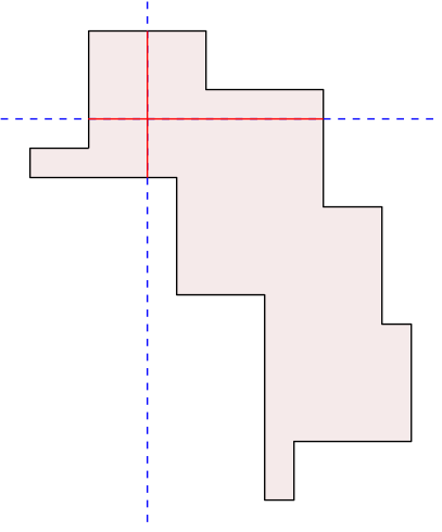
(a) Orthogonally Convex Polygon

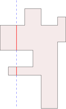
(b) Not Orthogonally Convex

Figure 13: Orthogonally Convex Polygons

It is easy to construct a simple orthogonal polygon having arbitrarily large number of knobs. However, we show that for orthogonally convex polygons, the number of knobs must be exactly $4$.

Lemma 5.26.

Any orthogonally convex polygon $P$ contains exactly $4$ knobs. Moreover, $P$ contains exactly one left knob, exactly one right knob, exactly one top knob and exactly one bottom knob.

Proof 5.27.

Existence. Consider the leftmost vertical line that intersects $P$ to form a non-empty vertical line segment of intersection. This must intersect with a vertical polygon edge of $P$ (otherwise the vertical line can be moved more to the left). Clearly these endpoints of this vertical polygon edge form a left knob (otherwise the vertical line can again be moved more to the left). Hence a left knob always exists. Symmetric arguments yield that a top knob, a bottom knob and a right knob exists as well.

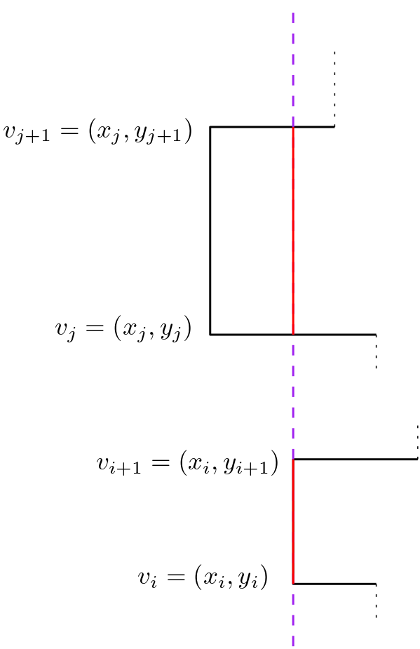
Figure 14: For proof of Lemma 5.26

Uniqueness. We will show that there cannot be two left knobs implying that there is exactly one left knob. For the sake of contradiction, consider that there are two left knobs $(v_{i},v_{i+1})$ and $(v_{j},v_{j+1})$ with $x_{i}=x_{i+1}\geq x_{j}=x_{j+1}$ (refer to Figure 14). Consider the vertical line $x=x_{i}$. This line intersects $P$ at the entire edge $(v_{i},v_{i+1})$ with the intercept the y coordinates being $[\min(y_{i},y_{i+1}),\max(y_{i},y_{i+1})]$. Now consider any curve lying inside $P$ with $v_{i}$ and $v_{j}$ as endpoints. This curve must also intersect the line $x=x_{i}$ (as $x_{j}\leq x_{i}$) at some y coordinate outside $[\min(y_{i},y_{i+1}),\max(y_{i},y_{i+1})]$. This means the intersection of the line $x=x_{i}$ with $P$ is not a single line segment, which contradicts the assumption that $P$ is orthogonally convex. Therefore, there can be exactly one left knob. Subsequently, by symmetric arguments this would mean that there is exactly one right knob, exactly one top knob and exactly one bottom knob.

Therefore, if we use Algorithm 5 to solve OPCS on orthogonally convex polygons, we can substitute $k=4$ in the analysis.

Corollary 5.28.

As orthogonally convex polygons have exactly $k=4$ knobs, Separating-Square-Recursion (Algorithm 5) takes $\mathcal{O}(n^{2})$ time to solve OPCS on orthogonally convex polygons.

6 Hardness Results for Polygons with Holes

In this Section, we consider the OPCSH problem. We consider the setting as described in [3], i.e. we need to solve OPCSH in orthogonal polygons, where the input consists of all $N$ lattice points lying in the polygon or on the boundary. In [3], a proof is given to show that OPCSH is NP-complete if the input size is polynomial in $N$. In this section, we fix an issue with the proof and state other results obtained as a consequence.

6.1 Issue with the existing proof

The proof in [3] for NP-completeness of OPCSH gives a reduction from Planar 3-CNF [8]. The reduction gives a polynomial time algorithm to reduce any Planar 3-CNF instance (say $\psi$) and transforms it to an instance of OPCSH. First the formula is negated to obtain $\phi=\neg\psi$, which is a formula in disjunctive normal form (DNF) due to De-Morgan’s law. This means that $\psi$ is satisfied if and only if $\phi$ evaluates to false on some truth assignment of the variables. Now, $\phi$ is reduced to an instance of OPCSH using three kinds of gadgets: wires, variable gadgets and junction gadgets. A variable gadget is introduced for each variable of $\phi$ and a junction gadget is introduced for each conjunction in $\phi$. Further wire gadgets (or simply wires) are introduced to ‘connect’ junction gadgets to variable gadgets.

The variable gadgets, wires and the junction gadgets shall be placed according to the formula $\phi$. For each variable gadget or each wire, it is easy to compute in polynomial time the minimum number of squares needed to cover the gadget. It is possible that some of the squares used for covering a wire may cover a region inside a junction gadget. Each variable gadget permits two kinds of covering (representing the two kinds of truth assignment to a variable in $\phi$). Let us denote these coverings by true-covering and false-covering, respectively - both coverings require the same number of squares. Similarly we can extend this observation to see that there are two ways in which a variable gadget and its adjacent wires can be covered optimally - and both coverings use the same number of squares. A combination of how a variable gadget is covered affects which portions of all its corresponding junction gadgets (i.e. gadgets for the and-clauses containing the corresponding variable in $\phi$) will be covered. We will keep the construction of variable gadgets and wires unchanged from the construction in [3]. Let $V$ be the number of squares required to cover all variable gadgets and $W$ be the number of squares required to cover all wire gadgets.

In [3], the authors claim that the junction gadgets (or simply, a junction) are such that, the minimum number of squares needed to cover a junction gadget is $12$ if all three variable gadgets corresponding to the and-clause are covered with a covering which makes the and-clause evaluate to true (i.e. true-covering if the variable appears non-negated in the clause, or false-covering if the variable is negated in the clause); otherwise the minimum number of squares needed is $13$. Therefore, the junctions act similar to and-gates. Now, if the total number of junctions be $j$, then [3] concludes by stating that $\psi$ is satisfiable if and only if the reduced instance can be covered with less than $(V+W+13j)$ squares; otherwise exactly $(V+W+13j)$ squares are required. Hence solving OPCSH would also solve Planar 3-CNF.

However, we take a deeper look into this reduction by performing a case work on the evaluated value of $\psi$ for possible truth assignments of variables.

• Case I, $\psi$ is true for all assignments. This implies $\phi=\neg\psi$ is false for all assignments. Since $\phi$ is in DNF, all assignments must render all and-clauses as false. Therefore, for all minimum covering of the variable gadgets, coverings all junctions would require $13$ squares. This means the minimum number of squares needed to cover such an instance is $V+W+13j$.

• Case II, $\psi$ is false for all assignments. This implies $\phi=\neg\psi$ is true for all assignments. Since $\phi$ is in DNF, all assignments must render at least one and-clauses as true. Therefore, for any arbitrary minimum covering of the variable gadgets, there would be at least one junction that can be covered with $12$ squares (while others take at most $13$ squares). This means the minimum number of squares needed to cover such an instance is less than $V+W+13j$.

• Case III, $\psi$ is true for some assignments and false for some. This implies $\phi=\neg\psi$ is also true for some assignments and false for some. Consider any such assignment such that $\phi$ is true and cover the variable clauses accordingly. Since $\phi$ is in DNF, this assignments must render at least one and-clauses as true. Therefore, if we cover the variable gadgets corresponding to such an assignment, there would be at least one junction that can be covered with $12$ squares (while others take at most $13$ squares). This means the minimum number of squares needed to cover such an instance is less than $V+W+13j$.

Therefore, the minimum number of squares to cover the reduced instance is equal to $V+W+13j$ if and only if $\psi$ is true for all assignments (Case I) and less than $V+W+13j$ otherwise. Therefore, solving OPCSH solves tautology for $\psi$ instead of satisfiablity. Moreover, tautology in a CNF formula can be checked in linear time (Since $\psi$ is a tautology if and only if for all clauses $c$ in $\phi$ there is a variable $x$ such that both $x$ and $\neg x$ appear in $c$). Hence this reduction does not prove NP-hardness of OPCSH.

6.2 Fixing the Construction

The issue in the NP-hardness reduction in [3] arose as the clauses require more number of squares when the literals of a clause do not all evaluate to true even if this assignment sets the clause to true.

We construct such a junction that requires $29$ squares if all three of its literals evaluate to false, whereas the junctions require $28$ squares when at least one literal evaluates to true. Therefore our modified junction behaves similar to an or-gate.

Recapping the Constructions of Variable Gadgets and Wires.

The construction due to [3] starts by defining even-lines (odd-lines) as horizontal lines with an even (odd) y-coordinate or a vertical line with an even (odd) x-coordinate. The construction of variable gadgets and wires follow the following properties.

• All maximal squares of variable gadgets and wires are $2\times 2$ in dimension.

• The wires connecting a variable gadget for a variable $x$, to a junction for a clause $c$, where $x$ appears non-negated in $c$ — connect to the variable gadget (as well as the junction) horizontally, and along two consecutive odd lines (i.e. an even line passes through the middle of such a connection). Refer to diagrams in  [3].

• The wires connecting a variable gadget for a variable $x$, to a junction for a clause $c$, where $x$ appears negated in $c$ — connect to the variable gadget (as well as the junction) horizontally, and along two consecutive even lines (i.e. an odd line passes through the middle of such a connection). Refer to diagrams in  [3].

• If a variable gadget for a variable $x$ is covered with a true-covering, then all wires connecting it to a junction for a clause $c$ where $x$ appears non-negated, will be covered in a way such that half a square protrudes out of destination and hence covers a part of the junction. Otherwise, for a false-covering, the entire junction would remain uncovered, even when the variable gadget and the wire are covered. Refer to diagrams in  [3].

• If a variable gadget for a variable $x$ is covered with a false-covering, then all wires connecting it to a junction for a clause $c$ where $x$ appears negated, will be covered in a way such that half a square protrudes out of destination and hence covers a part of the junction. Otherwise, for a true-covering, the entire junction would remain uncovered, even when the variable gadget and the wire are covered. Refer to diagrams in  [3].

We construct new junction gadgets along with these constructions of wires and variable gadgets in [3].

Modifying the Junction Gadgets.

We construct new junction gadgets as shown in Figure 15. Wires connect to these junction gadgets in the same way as described in [3].

(a) Junction for clauses of type $(x\vee y\vee z)$

(b) Junction for clauses of type $(x\vee\neg y\vee z)$

Figure 15: Modified junction

The junctions for clauses of type $(\neg x\vee\neg y\vee\neg z)$ can be constructed by shifting the gadget in Figure 15(a) vertically up by one square. Similarly the junctions for clauses of type $(\neg x\vee y\vee\neg z)$ can be constructed by shifting the gadget in Figure 15(b) vertically up by one square.

We now investigate minimal coverings of squares for each of these gadgets.

Lemma 6.1.

Each junction gadget requires $28$ squares to be covered when at least one literal in it evaluates to true. Otherwise the junction gadget requires $29$ squares to be covered.

Proof 6.2.

The following proof works for both the gadgets in Figure 15(a) and Figure 15(b). Both configurations are such that there are nine $4\times 4$ maximal squares due to convex vertices present due, and eleven $2\times 2$ squares necessary for joining with wire gadgets (Remark 3.5). Other than these $20$ squares, we analyse other valid squares needed to cover it fully.

In both gadgets, we can find eight blocks ($1\times 1$ regions) $p_{1},\ldots,p_{8}$, as shown in Figure 16, such that these are not covered by any of the $20$ previously placed squares (irrespective of the true/false values carried through the wires); and for $i\neq j$, $p_{i}$ and $p_{j}$ cannot be covered by a single valid square. This means at least $8$ more valid squares are required to cover the entire gadget. This means at least $28$ squares are required to cover the entire gadget (for any truth values being carried through the wires).

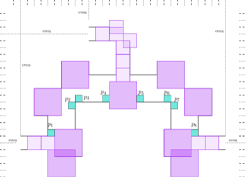
(a) $p_{1},\ldots,p_{8}$ for Figure 15(a)

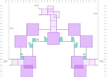
(b) $p_{1},\ldots,p_{8}$ for Figure 15(b)

Figure 16: Positions of $p_{1},\ldots,p_{8}$

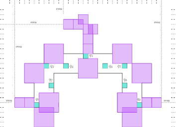
(a) $q_{1},\ldots,q_{9}$ for Figure 15(a)

(b) $q_{1},\ldots,q_{9}$ for Figure 15(b)

Figure 17: Positions of $q_{1},\ldots,q_{9}$

Further, if all wires contain a false value, we can find nine blocks ($1\times 1$ regions) $q_{1},\ldots,q_{9}$, as shown in Figure 17, such that these are not covered by any of the $20$ previously placed squares; and for $i\neq j$, $q_{i}$ and $q_{j}$ cannot be covered by a single valid square. This means at least $9$ more valid squares are required to cover the entire gadget. Therefore at least $29$ squares are required to cover the entire gadget when all wires contain a false value.

In Figure 18 and Figure 19, we indeed construct a set of $29$ valid squares covering the entire gadget when all three wires carry a false value, and a set of $28$ valid squares covering the entire gadget when at least one of the wires contain a true value. This construction proves that indeed $29$ squares and $28$ squares are precisely the minimum number of valid covering squares required to cover the gadgets if all literals are false, and at least one literal is true, respectively. This completes the proof.

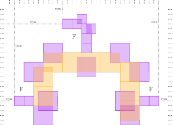
(a) $29$ squares when literals are $(F,F,F)$

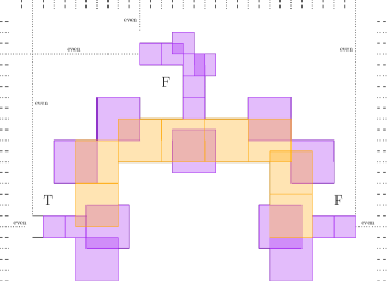
(b) $28$ squares when literals are $(F,F,T)$ or $(T,F,F)$

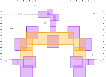
(c) $28$ squares when literals are $(T,F,T)$

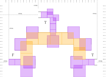
(d) $28$ squares when literals are $(F,T,T)$ or $(T,F,F)$

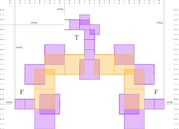
(e) $28$ squares when literals are $(F,T,F)$

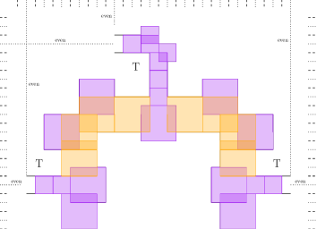
(f) $28$ squares when literals are $(T,T,T)$

Figure 18: Minimal covering of junctions in Figure 15(a)

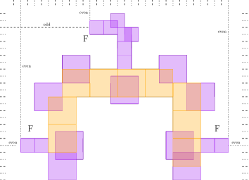
(a) $29$ squares when literals are $(F,F,F)$

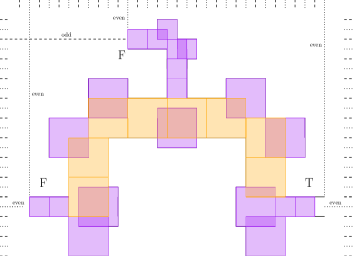
(b) $28$ squares when literals are $(F,F,T)$ or $(T,F,F)$

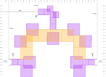
(c) $28$ squares when literals are $(T,F,T)$

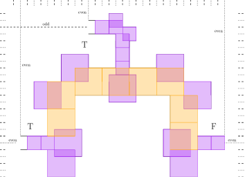
(d) $28$ squares when literals are $(F,T,T)$ or $(T,F,F)$

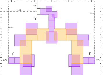
(e) $28$ squares when literals are $(F,T,F)$

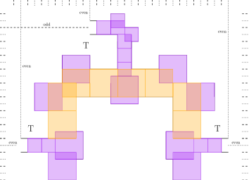
(f) $28$ squares when literals are $(T,T,T)$

Figure 19: Minimal covering of junctions in Figure 15(b)

Now, we complete the reduction from Planar 3-CNF (refer to [8]).

Completing the Reduction.

We consider an instance (a CNF boolean formula) $\psi$ of Planar 3-CNF. We construct variable gadgets (as in [3]) for each variable in $\psi$, and set up junctions ( Figure 15) for each clause in $\psi$ (we are working with $\psi$ directly, instead of working with $\phi=\neg\psi$ as done in [3]) and connect them with wires (as in [3]). Let $V+W$ be the squares required to cover all variable gadgets and wires.

Now, we analyse the three cases like before. Let $j$ be the number of junctions.

• Case I, $\psi$ is true for all assignments (satisfiable). Since $\psi$ is in CNF, all assignments must render all or-clauses as true (i.e. at least one literal in each clause is true). Therefore from Lemma 6.1, for all minimum covering of the variable gadgets, coverings all junctions would require a minimum of only $28$ valid squares. This means the minimum number of squares needed to cover such an instance is equal to $V+W+28j$.

• Case II, $\psi$ is false for all assignments (not satisfiable). Since $\psi$ is in CNF, all assignments must render at least one or-clause as false (i.e. at all literals in at least one clause is false). Therefore from Lemma 6.1, at least one junction requires a minimum of $29$ valid squares, where as others require at least $28$ valid squares for being covered. This means the minimum number of squares needed to cover such an instance is strictly more than $V+W+28j$.

• Case III, $\psi$ is true for some assignments and false for some (satisfiable). Consider any such assignment such that $\psi$ is true and cover the variable clauses accordingly. Since $\psi$ is in CNF, this assignments must render all or-clauses as true (i.e. at least one literal in each clause is true). Therefore from Lemma 6.1, for such a minimum covering of the variable gadgets, coverings all junctions would require $28$ squares. This means the minimum number of squares needed to cover such an instance is equal to $V+W+28j$.

This implies that $\psi$ is satisfiable if and only if the reduced instance has a minimum covering with exactly $V+W+28j$ squares. On the other hand, if $\psi$ is not satisfiable, then the minimum number of squares required to cover the reduced instance is strictly more than $V+Q+28j$. Since Planar 3-CNF is NP-hard, OPCSH must also be NP-hard. Finally, as any certificate can be verified in polynomial time using Algorithm 1, OPCSH is NP-complete.

Theorem 6.3.

The problem of covering orthogonal polygons with holes using minimum number of squares (OPCSH) is NP-complete (when the input is the set of all $N$ lattice points inside the orthogonal polygon).

Moreover, as both the answer $V+W+28j$ and the numerical value of the coordinates of each of the points is linear (polynomial) in the number $N$ of points inside the polygon, the problem is strongly NP-complete. Hence we can conclude the following.

Corollary 6.4.

OPCSH is strongly NP-complete. Therefore, there is no FPTAS scheme for OPCSH unless $\mbox{P}=\mbox{NP}$. That is, there is no $(1+\varepsilon)$-approximation scheme for arbitrarily small $\varepsilon$, such that runs in time $\mathcal{O}(poly(\frac{1}{\varepsilon},N))$, where $N$ is the number of lattice points inside the polygon.

Due to the structure of the reduced instance, we can also infer the following.

Corollary 6.5.

The following problems are NP-complete:

• The problem of finding a minimum square covering of polygons with holes, where all squares are restricted to have a side-length of at most $\eta$ is NP-complete whenever $\eta\geq 4$.

• The problem of finding the minimum square covering of polygons, where the squares can take side lengths from a set $\Lambda\subset\mathbb{N}$ is NP-complete, even if $|\Lambda|=2$.

Proof 6.6.

The results follow from the observation that the reduced instance from Planar 3-CNF only contains maximal squares of size $2\times 2$ and $4\times 4$, and from Observation 3.

Another immediate corollary of Theorem 6.3 is that fact that OPCSH is NP-hard when the $n$ vertices of the polygon constitute the input, instead of the $N$ lattice points lying inside. This is because the reduced instance had $n=\Theta(N)$. It turns out that OPCSH is in fact in the class NP, with $n$ vertices as input. This gives us the following result.

Corollary 6.7.

OPCSH is NP-complete when the input is the $n$ vertices.

Proof 6.8.

Theorem 6.3 immediately gives us that OPCSH is NP-hard when the input is the $n$ vertices.

To prove that OPCSH with $n$ vertices is in NP, we need to show a polynomial time verifier for a certificate. We consider the set of rec-packs to be a certificate, and we can do the following to check if these indeed form a valid covering:

• Check if each rec-pack lies inside the polygon. This can be checked in $\mathcal{O}(n)$ by checking if an arbitrary point in the rec-pack lies in the polygon, followed by ensuring that no polygon-edge intersects a rec-pack edge non-trivially.

• If all rec-packs lie in the polygon, we can use Algorithm 1 to check if they form a complete covering of the polygon. Algorithm 1 does generalize to polygons with holes as well.

This proves there there is in fact a polynomial time verifier for OPCSH.

7 Conclusion

In this paper, we answer an open problem in [3], of whether OPCS has an exact algorithm running in time polynomial in the number $n$ of vertices of the input orthogonal polygon without holes. Our exact algorithm for OPCS runs in $\mathcal{O}(n^{14})$ time. We further optimize the running time for orthogonal polygons with $n$ vertices and a small number of knobs $k$, by designing a recursive algorithm with running time $\mathcal{O}(n^{2}+k^{14}\cdot n)$. This gives us an $\mathcal{O}(n^{2})$ algorithm for solving OPCS on orthogonally convex polygons. We also correct some errors in the NP-hardness reduction for OPCSH given in [3]. A natural future direction is to study the problem with respect to covering of orthogonal polygons with other geometric objects like triangles, line segments, orthogonally convex polygons etc. and try to obtain an algorithm whose running time is polynomial in the number of vertices of the input polygon and not on the total number of interior points of the input polygon. Another interesting question directly related to our current work would be to find tight bounds for the number of rec-packs required to produce a minimum covering of an orthogonal polygon; our paper only proves an upper bound of $\mathcal{O}(n^{2})$ rec-packs required to produce a minimum covering of an entire polygon.

References

- [1] Michael O. Albertson and Claire J. O’Keefe. Covering regions with squares. SIAM Journal on Algebraic Discrete Methods, 2(3):240–243, 1981. arXiv:https://doi.org/10.1137/0602026, doi:10.1137/0602026.
- [2] V. S. Anil Kumar and H. Ramesh. Covering rectilinear polygons with axis-parallel rectangles. In Proceedings of the Thirty-First Annual ACM Symposium on Theory of Computing, STOC ’99, page 445–454, New York, NY, USA, 1999. Association for Computing Machinery. doi:10.1145/301250.301369.
- [3] L. J. Aupperle, H. E. Conn, J. M. Keil, and Joseph O’Rourke. Covering orthogonal polygons with squares. Proc. 26th Allerton Conf. Commun. Control Comput., 1988. URL: https://www.science.smith.edu/~jorourke/Papers/ConnJORsquares.pdf.
- [4] Reuven Bar-Yehuda. Covering polygons with squares. 2014. URL: https://api.semanticscholar.org/CorpusID:50721774.
- [5] Jean R. S. Blair and Barry Peyton. An introduction to chordal graphs and clique trees. In Alan George, John R. Gilbert, and Joseph W. H. Liu, editors, Graph Theory and Sparse Matrix Computation, pages 1–29, New York, NY, 1993. Springer New York.
- [6] J.C. Culberson and R.A. Reckhow. Covering polygons is hard. In [Proceedings 1988] 29th Annual Symposium on Foundations of Computer Science, pages 601–611, 1988. doi:10.1109/SFCS.1988.21976.
- [7] Fanica Gavril. Algorithms for minimum coloring, maximum clique, minimum covering by cliques, and maximum independent set of a chordal graph. SIAM J. Comput., 1:180–187, 1972. URL: https://api.semanticscholar.org/CorpusID:1111479.
- [8] David Lichtenstein. Planar formulae and their uses. SIAM Journal on Computing, 11(2):329–343, 1982. doi:10.1137/0211025.
- [9] Dipen Moitra. Finding a minimal cover for binary images: An optimal parallel algorithm. Algorithmica, 6(5):624–657, 1991. doi:10.1007/BF01759065.
- [10] J. O’Rourke. Art Gallery Theorems and Algorithms. International series of monographs on computer science. Oxford University Press, 1987. URL: https://books.google.co.in/books?id=aPZQAAAAMAAJ.